Embed Size (px)
Citation preview
2003 Royal Statistical Society 1369–7412/03/65585
J. R. Statist. Soc. B (2003)65, Part 3, pp. 585–618
A theory of statistical models for Monte Carlointegration
A. Kong,
deCODE Genetics, Reykjavik, Iceland
P. McCullagh,
University of Chicago, USA
X.-L. Meng
Harvard University, Cambridge, USA
and D. Nicolae and Z. Tan
University of Chicago, USA
[Read before The Royal Statistical Society at a meeting organized by the Research Section onWednesday, December 11th, 2002 , Professor D. Firth in the Chair ]
Summary. The task of estimating an integral by Monte Carlo methods is formulated as a sta-tistical model using simulated observations as data. The difficulty in this exercise is that weordinarily have at our disposal all of the information required to compute integrals exactly bycalculus or numerical integration, but we choose to ignore some of the information for simplicityor computational feasibility. Our proposal is to use a semiparametric statistical model that makesexplicit what information is ignored and what information is retained. The parameter space inthis model is a set of measures on the sample space, which is ordinarily an infinite dimensionalobject. None-the-less, from simulated data the base-line measure can be estimated by maxi-mum likelihood, and the required integrals computed by a simple formula previously derived byVardi and by Lindsay in a closely related model for biased sampling.The same formula was alsosuggested by Geyer and by Meng and Wong using entirely different arguments. By contrast withGeyer’s retrospective likelihood, a correct estimate of simulation error is available directly fromthe Fisher information. The principal advantage of the semiparametric model is that variancereduction techniques are associated with submodels in which the maximum likelihood estima-tor in the submodel may have substantially smaller variance than the traditional estimator. Themethod is applicable to Markov chain and more general Monte Carlo sampling schemes withmultiple samplers.
Keywords: Biased sampling model; Bridge sampling; Control variate; Exponential family;Generalized inverse; Importance sampling; Invariant measure; Iterative proportional scaling;Log-linear model; Markov chain Monte Carlo methods; Multinomial distribution; Normalizingconstant; Semiparametric model; Retrospective likelihood
1. Normalizing constants and Monte Carlo integration
Certain inferential problems arising in statistical work involve awkward summation or highdimensional integrals that are not analytically tractable. Many of these problems are such that
Address for correspondence: P. McCullagh, Department of Statistics, University of Chicago, 5734 UniversityAvenue, Chicago, IL 60657-1514, USA.E-mail: [email protected]
586 A. Kong, P. McCullagh, X.-L. Meng, D. Nicolae and Z. Tan
only ratios of integrals are required, and it is this class of problems with which we shall beconcerned in this paper. To establish the notation, let Γ be a set, let µ be a measure on Γ, let{qθ} be a family of functions on Γ and let
c.θ/ =∫
Γqθ.x/ dµ:
Our goal is ideally to compute exactly, or in practice to estimate, the ratios c.θ/=c.θ′/ for allvalues θ and θ′ in the family. The family may contain a reference function qθ0 whose integral isknown, in which case the remaining integrals are directly estimable by reference to the standard.Our theory accommodates but does not require such a standard. For an estimator to be useful,an approximate measure of estimation error is also required.We refer to c.θ/ as the normalizing constant associated with the function qθ.x/. In particular,
if qθ is non-negative and 0 < c.θ/ <∞,
dPθ.x/ = qθ.x/ dµ=c.θ/is a probability distribution on Γ. For the method to work, the family must contain at least onenon-negative function qθ, but it is not necessary that all of them be non-negative. Dependingon the context and on the functions qθ, the normalization constant might represent anythingfrom a posterior expectation in a Bayesian calculation to a partition function in statisticalphysics.Observations simulated from one or more of these distributions are the key ingredient in
Monte Carlo integration. We assume throughout the paper that techniques are available tosimulate from Pθ without computing the normalization constant. At least initially, we assumethat these techniques generate a stream of independent observations from Pθ.
At first glance, the problem appears to be an exercise in calculus or numerical analysis, andnot amenable to statistical formulation. After all, statistical theory does not seek to avoid esti-mators that are difficult to compute; nor is it inclined to opt for inferior estimators because theyare convenient for programming. So it is hard to see how any efficient statistical formulationcould avoid the obvious and excellent estimator c.θ/ = ∫
qθ.x/ dµ, which has zero variance andrequires no simulated data.This paper demonstrates that the exercise can nevertheless be formulated as a model-based
statistical estimation problem in which the parameter space is determined by how much infor-mation we choose to ignore. In effect, the statistical model serves to estimate that part of theinformation that is ignored and uses the estimate to compute the required integrals in a mannerthat is asymptotically efficient given the information available. Neither the nature nor the extentof the ignored information is predetermined. By judicious use of group invariant submodelsand other submodels, the amount of information ignored may be controlled in such a way thatthe simulation variance is reduced with little increase in computational effort.The literature on Monte Carlo estimation of integrals is very extensive, and no attempt will
be made here to review it. For good summaries, see Hammersley and Hanscomb (1964), Ripley(1987), Evans and Swartz (2000) or Liu (2001). For overviews on the computation of normal-izing constants, see DiCiccio et al. (1997) or Gelman and Meng (1998).
2. Illustration
The following examplewith sample spaceΓ = R×R+ is sufficiently simple that the integrals canbe computed analytically. Nevertheless, it illustrates the gains that are achievable by choice of
Statistical Models for Monte Carlo Integration 587
design and by choice of submodel. ThreeMonte Carlo techniques are described and compared.Suppose that we need to evaluate the integrals over the upper half-plane
cσ =∫
Γ
dx1 dx2{x21 + .x2 + σ/2}2
for σ ∈ {0:25, 0:5, 1:0, 2:0, 4:0}. It is conventional to take µ to be Lebesgue measure, so thatqσ.x/ = 1={x21 + .x2 + σ/2}2. As it happens, the distribution Pσ has mean .0,σ/ with infinitevariances and covariances. Consider first an importance sampling design in which a stream ofindependent observations x1, : : :, xn is made available from the distribution P1. The importancesampling estimator of cσ=c1 is
cσ=c1 = n−1 ∑qσ.xi/=q1.xi/:
By applying the results from Section 4, we find on the basis of n = 500 simulations that thematrix
V = n−1
4:411 1:491 0:000 −0:601 −0:8211:491 0:641 0:000 −0:383 −0:5820:000 0:000 0:000 0:000 0:000
−0:601 −0:383 0:000 0:578 1:273−0:821 −0:582 0:000 1:273 3:591
is such that the asymptotic variance of log.cr=cs/ is equal to Vrr+ Vss−2Vrs for r, s ∈ {0:25, 0:5,1:0, 2:0, 4:0}. The individual components cr are not identifiable in the model and the estimatesdo not have a variance, asymptotic or otherwise. The estimated variances of the 10 pairwiselogarithmic contrasts range from 0:6=n to 9:6=n, with an average of 3:6=n. The matrix V isobtained from the observed Fisher information, so a different simulation will yield a slightlydifferent matrix.Suppose as an alternative that it is feasible to simulate from any or all of the distributions Pσ,
as in Geyer (1994), Hesterberg (1995), Meng and Wong (1996) or Owen and Zhou (2000). Var-ious simulation designs, also called defensive importance sampling or bridge sampling plans,can now be considered in which nr observations are generated from Pr. These are called thedesign weights, or bridge sampling weights. For simplicity we consider the uniform design inwhich nr = n=5. The importance sampling estimator must now be replaced by the more generalmaximum likelihood estimator derived in Section 3, which is obtained by solving
cσ =n∑i=1
qσ.xi/∑snsc
−1s qs.xi/
: .2:1/
The asymptotic covariance matrix of log.c/ obtained from a sample of n = 500 simulatedobservations using equation (4.2) is
V ′ = n−1
2:298 0:974 −0:263 −1:197 −1:8110:974 0:668 0:077 −0:588 −1:131
−0:263 0:077 0:239 0:117 −0:170−1:197 −0:588 0:117 0:690 0:979−1:811 −1:131 −0:170 0:979 2:132
:
In using this matrix, it must be borne in mind that c ≡ λc for every positive scalar λ, so onlycontrasts of log.c/ are identifiable. The estimated variances of the 10 pairwise logarithmic
588 A. Kong, P. McCullagh, X.-L. Meng, D. Nicolae and Z. Tan
contrasts range from 0:7=n to 8:1=n, with an average of 3:0=n. The average efficiency factorof the uniform design relative to the preceding importance sampling design is convenientlymeasured by the asymptotic variance ratio 3:6=3:0 = 1:2.A third Monte Carlo variant uses a submodel with a reduced parameter space consisting of
measures that are invariant under group action. Details are described in Section 3.3, but theoperation proceeds as follows. Consider the two-element group G = ±1 in which the inversiong = −1 acts on Γ by reflection in the unit circle
g : .x1, x2/ → .x1, x2/=.x21 + x22/:
By construction, g2 = 1 and g−1 = g, so this is a group action. Lebesgue measure is not invari-ant and is thus not in the parameter space as determined by this action. However, the measureρ.dx/ = dx1 dx2=x22 is invariant, so we compensate by writing
q.x;σ/ = x22={x21 + .x2 + σ/2}2
for the new integrand, and cσ = ∫Γ q.x;σ/ dρ. The submodel estimator is the same as equation
(2.1), but with q replaced by the group average
q.x;σ/ = 12 q.x;σ/+ 1
2 q.gx;σ/:
With a uniform design and n = 500 observations, the estimated variance matrix of log.c/ is
V ′′ = n−1
0:202 −0:093 −0:216 −0:093 0:202−0:093 0:045 0:097 0:045 −0:093−0:216 0:097 0:239 0:097 −0:216−0:093 0:045 0:097 0:045 −0:0930:202 −0:093 −0:216 −0:093 0:202
:
The variances of the 10 pairwise logarithmic contrasts range from 0 to 0:87=n with an averageof 0:37=n. For reasons described in Section 3.3, the two ratios c0:25=c4 and c0:5=c2 are estimatedexactly with zero variance. Relative to the preceding Monte Carlo estimator, group averag-ing reduces the average simulation variance of contrasts by an efficiency factor of 8.1. By thiscomparison, n simulated observations using the group-averaged estimator are approximatelyequivalent to 8nobservations using the estimator (2.1)with the samedesignweights, butwithoutgroup averaging.To achieve efficiency gains of this magnitude, it is not necessary to use a large group, but it
is necessary to have a good understanding of the integrands in a qualitative sense, and to selectthe group action accordingly. If the group action had been chosen so that g.x1,x2/ = .−x1,x2/the gain in efficiency would have been zero. Arguably, the gain in efficiency would be negativebecause of the slight increase in computational effort.Given observations simulated by any of the preceding schemes, equation (2.1), or the group-
averaged version, can also be used for the estimation of integrals such as
c′σ =∫
Γ
log.x21 + x22/ dx1 dx2{x21 + .x2 + σ/2}2
in which the integrand is not positive, and there is no associated probability distribution. In thisextended version of the problem, 10 integrals are estimated simultaneously, and c′σ=cσ is theexpected value of log |X2
1+X22|whenX∼Pσ. For this example, cσ =π=4σ2, and c′σ=cσ = 2 log.σ/.
The general theory described in the next section covers integrals of this sort, and the Fisherinformation also provides a variance estimate.
Statistical Models for Monte Carlo Integration 589
3. A semiparametric model
3.1. Problem formulationThe statistical problem is formulated as a challenge issued by one individual called the simulatorand accepted by a second individual called the statistical analyst. In practice, these typically aretwo personalities of one individual, but for clarity of exposition we suppose that two distinctindividuals are involved. The simulator is omniscient, honest and secretive butwilling to providedata in essentially unlimited quantity. Partial information is available to the analyst in the formof a statistical model and the data made available by the simulator.Let q1, : : :,qk be real-valued functions on Γ, known to the analyst, and let µ be any non-
negative measure on Γ. The challenge is to compute the ratios cr=cs, where each integral cr =∫Γ qr.x/ dµ is assumed to be finite, i.e. we are interested in estimating all ratios simultaneously,where qr.x/= qθr .x/, using the notation of Section 1. Assume that there is at least one non-negative function qr such that 0<cr <∞, and that nr observations from the weighted distribu-tion
Pr.dx/ = c−1r qr.x/ µ.dx/ .3:1/
are made available by the simulator at the behest of the analyst. The analyst’s design vector.n1, : : :,nk/ has at least one r such that nr > 0. Typically, however, many of the functions qr aresuch that nr = 0. For these functions, the non-negativity condition is not required.Different versions of the problem are available depending on what is known to the analyst
about µ. Four of these are now described.
(a) If µ is known, e.g. if µ is Lebesguemeasure, the constants can, in principle, be determinedexactly by integral calculus.
(b) If µ is known up to a positive scalar multiple, the constants can be determined modulothe same scalar multiple, and the ratios can be determined exactly by integral calculus.
(c) If µ is completely unknown, neither the constants nor their ratios can be determined bycalculus alone. Nevertheless, the ratios can be estimated consistently from simulated databy using a slight modification of Vardi’s (1985) biased sampling model.
(d) If partial information is available concerning µ, neither the constants nor their ratios canbe determined by calculus. Nevertheless, partial information may permit a substantialgain of efficiency by comparison with (c).
As an exercise in integral calculus, the first and second versions of the problem are not con-sidered further in this paper.
3.2. A full exponential modelIn this section, we focus on a semiparametricmodel inwhich the parameterµ is ameasure or dis-tribution on Γ, completely unknown to the analyst. The simulator is free to choose any measureµ, and the analyst’s estimate must be consistent regardless of that choice. The parameter spaceis thus the set Θ of all non-negative measures on Γ, not necessarily probability distributions,and the components of interest are the linear functionals
cr =∫
Γqr.x/ dµ: .3:2/
The state spaceΓ in the following analysis is assumed tobe countable; themore general argumentcovering uncountable spaces is given by Vardi (1985) in a model for biased sampling.
590 A. Kong, P. McCullagh, X.-L. Meng, D. Nicolae and Z. Tan
We suppose that simulated data are available in the form .y1,x1/, : : :, .yn,xn/, in which thepairs are independent, yi ∈ {1, : : :, k} is determined by the simulation design and xi is a randomdraw from the distribution Pyi . Then for each draw x from the distribution Pr the likelihoodcontribution is
Pr.{x}/ = c−1r qr.x/ µ.{x}/:
The full likelihood at µ is thus
L.µ/ =n∏i=1Pyi.{xi}/ =
n∏i=1
µ.{xi}/c−1yiqyi .xi/:
It is helpful at this stage to reparameterize themodel in terms of the canonical parameter θ ∈ RΓ
given by θ.x/ = log[µ.{x}/]. Let P be the empirical measure on Γ placing mass 1=n at each datapoint. Ignoring additive constants, the log-likelihood at θ is
n∑i=1
θ.xi/−k∑s=1ns log{cs.θ/} = n
∫Γθ.x/ dP −
k∑s=1ns log{cs.θ/}: .3:3/
Although it may appear paradoxical at first, the canonical sufficient statistic P , the empiricaldistribution of the simulated values {x1, : : :, xn}, ignores a part of the data that might be con-sidered highly informative, namely the association of distribution labels with simulated values.In fact, all permutations of the labels y give the same likelihood. The likelihood function isthus unaffected by reassignment of the distribution labels y to the draws x. This point waspreviously noted by Vardi (1985), section 6. Thus, under the model as specified, or under anysubmodel, the association of draws with distribution labels is uninformative. The reason forthis is that all the information in the labels for estimating the ratios is contained in the designconstants {n1, : : :,nk}.As is evident from equation (3.3), the model is of the full exponential family type with
canonical parameter θ, and canonical sufficient statistic P . The maximum likelihood estimateof µ, obtained by equating the canonical sufficient statistic to its expectation, is
nP .dx/ =k∑s=1nsc
−1s qs.x/ µ.dx/,
where dx = {x}. Thus
µ.dx/ = nP.dx//k∑s=1nsc
−1s qs.x/, .3:4/
where cs is the maximum likelihood estimate of cs. Note that µ is supported on the data values{x1, : : :,xn}, but the atoms at these points are not all equal. From the integral definition of cr,we have
cr =∫
Γqr.x/ dµ =
n∑i=1
qr.xi/
k∑s=1nsc
−1s qs.xi/
: .3:5/
In principle, it is necessary to check that there exists in the parameter space ameasure µ such thatthese equations are satisfied, which is a non-trivial exercise for certain extreme configurationsof the observations. Fortunately existence and uniqueness have been studied in great detail forVardi’s biased sampling model (Vardi, 1985), which is essentially mathematically equivalent.
Statistical Models for Monte Carlo Integration 591
Although P is uniquely determined, µ is determined modulo an arbitrary positive multiple,and the constants cr are determined modulo the same positive multiple. In other words, theset of estimable parametric functions may be identified with the space of logarithmic contrastsΣ ar log.cr/ in which Σ ar = 0. This is clear from equation (3.1), which implies that the problemof ratio estimation is invariant under the transformation qr.x/ → α.x/ qr.x/, where α is strictlypositive on Γ.The computational algorithm suggested by equation (3.5) is iterative proportional scaling
(Deming and Stephan, 1940; Bishop et al., 1975) applied to the n× k array {nr qr.xi/} in sucha way that, after rescaling,
nr qr.xi/ → nr qr.xi/ µ.xi/=cr,
each row total is 1 and the rth column total is nr. The special case k = 1, called importancesampling, corresponds to the Horvitz–Thompson estimator (Horvitz and Thompson, 1952),which is widely used in survey sampling to correct for unequal sampling probabilities. Wemightexpect to find the more general estimator (3.5) in use for combining data from one or moresurveys that use different known sampling probabilities. Possibly this exercise is not of interestin survey sampling. In any event, the estimator does not occur in Firth and Bennett (1998) or inPfeffermann et al. (1998), which are concerned with unequal selection probabilities in surveys.The normalized version of equation (3.4) has been obtained by Vardi (1985) and by Lindsay
(1995) in a nonparametricmodel for biased sampling. In his discussion of Vardi (1985),Mallows(1985) pointed out the connection with log-linear models and explained why the algorithm con-verges. These biased sampling models are not posed asMonte Carlo estimation, but the modelsare equivalent apart from the restriction of the parameter space to probability distributions. Forfurther details, including connectivity and support conditions for existence and uniqueness, seeVardi (1985) or Gill et al. (1988). These conditions are assumed henceforth.The preceding derivation assumes that Γ is countable, so counting measure dominates all
others. If Γ is not countable, no dominating measure exists. Nevertheless, the likelihood has auniquemaximum given by equation (3.4) provided that the connectivity and support conditionsare satisfied. This maximizingmeasure has finite support, and themaximum likelihood estimateof c is given by equation (3.5).
3.3. Symmetry and group invariant submodelsIn practice, we invariably ‘know’ that the base-line measure is either counting measure orLebesgue measure. The method described above completely ignores such information. As aresult, the conclusions apply equally to discrete sample spaces, finite dimensional vector spaces,metric spaces, product spaces and arbitrary subsets thereof. On the negative side, if the base-line measure does have symmetry properties that are easily exploited, the estimator may beconsiderably less efficient than it need be.To see how symmetries might be exploited, let G be a compact group acting on Γ in such a
way that the base-line measure µ is invariant: µ.gA/=µ.A/ for each A⊂ Γ and each g ∈ G.For example, G might be the orthogonal group, a permutation group or any subgroup. In thisreduced model, the parameter space consists only of measures that are invariant under G. Thelog-likelihood function (3.3) simplifies because θ.x/ = θ.gx/ for each g ∈ G, and the minimalsufficient statistic is reduced to the symmetrized empirical distribution function P G
P G.A/ = aveg∈G
{P .gA/}
for each A⊂ Γ. If G is finite and acts freely, P G has mass 1=n|G| at each of the transformed
592 A. Kong, P. McCullagh, X.-L. Meng, D. Nicolae and Z. Tan
sample points gxi with g ∈ G. In a rough sense, the effective sample size is increased by a factorequal to the average orbit size. The maximum likelihood estimate of µ, obtained by equatingthe minimal sufficient statistic to its expectation, is
n P G.dx/ =k∑s=1nsc
−1s qs.x/ µ.dx/,
where
qs.x/ = aveg∈G
{qs.gx/}: .3:6/
In other words, the estimates from the submodel are still given by equations (3.4) and (3.5), butwith qs replaced by the group average qs, and P replaced by P G. The group-averaged estimatormay be interpreted as Rao–Blackwellization given the orbit, so group averaging cannot increasethe variance of µ or of the linear functionals cr (Liu (2001), section 2.5.5).From the estimating equation point of view, the submodel replaces equation (3.2) by
cr =∫
Γqr.x/ dµ, .3:7/
which is a consequence of the assumption that µ is G invariant. However, if we proceed withequation (3.7) directly as with equation (3.2), it would appear that we need draws from
Pr.dx/ = c−1r qr.x/ µ.dx/,
rather thanPr.dx/. Althoughwe can easily draw xi from Pyi by randomly drawing a g fromG andsetting xi= gxi, this step is unnecessary because Pyi is invariant under G, and thus Pyi .{xi}/ =Pyi .{xi}/. Provided that G is sufficiently small that the group averaging in equation (3.6) repre-sents a negligible computational cost, the submodel estimator is no more difficult to computethan the original c. Consequently, the submodel is most useful if G is a small finite group. If Gis the orthogonal group, aveg∈G{qs.gx/} is the average with respect to Haar measure over aninfinite set. This is usually a non-trivial exercise in calculus or numerical integration, preciselywhat we had sought to avoid by simulation.With a judicious choice of group action, the potential gain in efficiency can be very large.
As an extreme example, suppose that the distributions Pr are such that for each r there existsa g ∈ G such that Pr.A/=P1.gA/ for every measurable A⊂ Γ. Then qr.x/=qs.x/ is a constantindependent of x for all r and s, and the ratios of normalizing constants are estimated exactlywith zero variance. This effect is evident in the example in Section 2 in which X∼Pσ impliesgX∼P1=σ. In practice, such a group action may be hard to find, but it is often possible tofind a group such that there is substantially more overlap among the symmetrized distribu-tions Pr.A/ = aveg∈G{Pr.gA/} than among the original {Pr}. For location–scale models withparameter .µ,σ/, reflection in the circle of radius σ centred at .µ, 0/ is sometimes effective forintegrals of likelihood functions or posterior distributions.Although a symmetrized estimator using a reflection such as q.x/= {q.x/ + q.−x/}=2 may
remind us of the antithetic principle to reduce Monte Carlo error, these two methods arefundamentally different. The antithetic principle exploits symmetry in the sampling distribu-tions, whereas group averaging utilizes the symmetry in the base-line measure. In addition, theeffectiveness of using antithetic variates depends on the form of the integrand (e.g. q2=q1), asa non-linear function can make antithetic variates worse than the standard estimator (3.5) (seeCraiu and Meng (2004)). In contrast, group averaging can do no harm regardless of the formof the integrand.
Statistical Models for Monte Carlo Integration 593
The importance link function method ofMacEachern and Peruggia (2000) has some featuresin common with group averaging, but the construction and the implementation are different inmajor ways. Group structure has also been used by Liu and Sabatti (2000), but for a differentpurpose, to improve the rate of mixing in Gibbs sampling.Group averaging has been discussed by Evans and Swartz (2000), page 191, as a method
of variance reduction for importance sampling. Although the aims are similar, the details areentirely different. Evans and Swartz considered only subgroups of the symmetry group of theimportance sampler. That is to say, the group action preserves both Lebesgue measure andthe importance sampling distribution. By contrast, our method is geared towards more generalbridge sampling designs, and the group action is not on the sampling distributions but on thebase-line measures. In our model, no preferential status is accorded to Lebesgue measure or toany particular sampler, so it is not necessary that the group action should preserve either. Onthe contrary, it is desirable that the group action should mix the distributions thoroughly tomake the averaged distributions as similar as possible.
3.4. Projection and linear submodelsUp to this point, the analysis has treated the k functions q1, : : :,qk in a symmetric mannereven where the design constants {n1, : : :,nk} are not equal. In practice, there may be substantialasymmetries that can be exploited to reduce simulation error. In the simplest case, it may beknown that two of the normalizing constants are equal, say c2 = c3. The reduced parameterspace is then the set of measures µ such that
∫.q2 − q3/ dµ = 0. Ideally, we would like to
estimate µ by maximum likelihood subject to this homogeneous linear constraint. Even when itexists and is unique, the maximum likelihood estimator in this submodel is unlikely to be costeffective, so we seek a simple one-step alternative by linear projection.Let c be the unconstrained estimator from equation (3.5) or the group-averaged version in
Section 3.3, and let V be the asymptotic variance matrix of log.c/ as given in equation (4.2). Weconsider a submodel inwhich c lies in the subspaceX ⊂ Rk. For example, a single homogeneousconstraint among the constants gives rise to a subspace X of dimension k − 1, and a matrix Xof order k × .k − 1/ whose columns span X .Ignoring statistical error in the asymptotic variancematrix cov.c/=CVC, whereC= diag.c/,
the weighted least squares projection is
c = X.XTC−1V−C−1X/−XTC−1V−1, .3:8/
where 1 is the constant vector with k components. See, for example, Hammersley and Hans-comb (1964), section 5.7. Provided that all generalized inverses are reflexive, i.e. V−V V− = V−,the asymptotic variance matrix is
cov.c/ = X.XTC−1V−C−1X/−XT:
As always, only ratios of cs are estimable in the submodel.It is perhaps worth mentioning by way of clarification the precise role of the control variates
when the objective is to estimate a single ratio c1=c2. Suppose that k = 3 and that the designconstants are .0,n, 0/, so all observations are generated from P2. Then the importance samplingestimator c1=c2 from equation (3.5) has asymptotic variance O.n−1/. Suppose now that P1 isin fact a mixture of P2 and P3, so q1 = α2q2 + α3q3, this being the reason for including q3 as acontrol variate such that
∫.q2 − q3/ dµ = 0. Then
594 A. Kong, P. McCullagh, X.-L. Meng, D. Nicolae and Z. Tan
c1 =∫q1.x/ dµ =
∫.α2q2 + α3q3/ dµ
= α2c2 + α3c3
is a linear combination of c2 and c3, so the covariance matrix of c has rank 2. After projection,c2 = c3 and c1 = .α2 + α3/c2, so c1=c2 = α2 + α3 is estimated with zero error. The coefficientsα2 and α3 are immaterial and need not be positive.It is evident that projection cannot increase simulation variance, but it is not evident that
the potential for reduction in simulation error by projection is very great. Indeed, if we areinterested primarily in estimating c1=c0, the reduction is typically not worthwhile unless thecontrol variates q2,q3, : : : are chosen carefully. The way in which this may be done for Bayesianposterior calculations is discussed in Section 5. Efficiency factors of the order of 5–10 appearto be routinely achievable.The discussion of control variates by Evans and Swartz (2000) involves subtraction rather
than projection, so the technique is different from that proposed above. The algebra in sec-tion 5.7 of Hammersley and Hanscomb (1964) and in Rothery (1982), Ripley (1987) and Glynnand Szechtman (2000) is, in most respects, equivalent to the projection method. There are somedifferences but these are mostly superficial, starting with the complication that only ratios areidentifiable in our models and submodels. The main difference in implementation is that ourlikelihood method automatically provides a variance matrix, so no preliminary experiment isrequired to estimate the coefficients in the projection. Glynn and Szechtman (2000), section 8,also noted that the required projection is a linear approximation to the nonparametricmaximumlikelihood estimator.
3.5. Log-linear submodelsMost sets that arise in statistical applications have a large amount of structure that can poten-tially be exploited in the construction of submodels. For example, the spaces arising in geneticproblems related to the coalescentmodel have a tree structure withmeasured edges. A submodelmay be useful for Monte Carlo purposes if the estimate under the submodel is easy to computeand has substantially reduced variance. The following example illustrates the principle as itapplies to spaces having a product structure.If Γ = Γ1 × : : : × Γl is a product set, it is natural to consider the submodel consisting of
product measures only, i.e. µ = µ1 × : : : × µl, in which µj is a measure on Γj. Then each x ∈ Γhas components .x1, : : :, xl/, and θ.x/ = θ1.x1/+ : : : + θl.xl/ in an extension of the notation ofSection 3.2. The sufficient statistic in equation (3.3) is reduced to the list of l marginal empiricaldistribution functions, and the resulting model is equivalent to the additive log-linear model(main effects only) for an l-dimensional contingency table, or l+1 dimensional if the design hasmore than one sampler. No closed form estimator is available unless the design is such that, foreach nr > 0, the function qr.x/ is expressible as a product qr.x/ = qr1.x1/ : : : qrl.xl/. Then eachsampler generates observations with independent components, so µj is given by equation (3.4),applied to the jth component of x. The component measures µ1, : : :, µl are then independent.In certain circumstances, the component setsΓ1, : : :,Γl are isomorphic, in which case wewrite
Γl instead of Γ. It is then natural to restrict the parameter space to symmetric product measuresof the form µl. Suppose, for example, that we wish to compute the integrals
cθ =∫
R2exp{−.x1 − θ/2=2 − .x2 − θ/2=2 − x21x22=2} dx1 dx2
for various values of θ in the range .0, 4/. These constitute a subfamily of distributions consid-
Statistical Models for Monte Carlo Integration 595
ered byGelman andMeng (1991), whose conditional distributions areGaussian. The parameterspace in the submodel is the set of symmetric productmeasuresµ×µ, soµ is ameasure onR. Fora sampler, it is convenient to take any distribution with density f onR, or the product distribu-tion onR2. The numerical values reported here are based on the standard Cauchy sampler. Themaximum likelihood estimate of µ on R has mass 1=nf.xi/ at each data point, so the maximumlikelihood estimate of µ2 on R2 has mass {n2f.xi/ f.xj/}−1 at each ordered pair .xi,xj/ in thesample.We find that the submodel estimator based on n simulated scalar observations is roughlyequivalent in terms of statistical efficiency to 3n=2 bivariate observations in the unconstrainedmodel. In principle, therefore, the crude importance sampling estimator can be improved by afactor of 3 without further data. On the negative side, the submodel estimator of cθ
cθ =∫qθ.x, x′/ dµ.x/ dµ.x′/
is the sum of n2 terms, as opposed to n terms in the unconstrained model. In terms ofcomputational effort, therefore, the importance sampling estimator is superior. The submodelestimator is not cost effectiveunless the simulations are thedominant time-consumingpart of thecalculation.There is one additional circumstance inwhich the submodel estimator achieves a gain in statis-
tical efficiency that is sufficient to offset the increase in computational effort. If two functions qrand qs are such that the one-dimensional marginal distributions of Pr are the same as the one-dimensional marginal distributions of Ps, the estimated ratio cr=cs has a variance that is o.n−1/,i.e.
n var{log.cr=cs/} → 0
as n → ∞. Simulation results indicate that the rate of decrease is O.n−2/. This phenomenoncan be observed if we replace the preceding family of integrands by the family exp.−x21 − x22 +2θx1x2/ for −1 < θ < 1.
3.6. Markov chain modelsThe model in this section assumes that a sequence of draws constitutes an irreducible Markovchain having known transition density q.·; x/with respect to the unknownmeasureµ onΓ. If thedesign calls for multiple chains, the transition densities are denoted by qr.·; x/ for r = 1, : : :, k. Itis not necessary that the chain be in equilibrium; nor is it necessary that the chain be constructedto have a particular stationary distribution. Under this new model, a draw is a chain of length lwith distribution P.l/r . The likelihood may be expressed as the product of l factors, the first threeof which are
Pr.dx1/ = c−1r qr.x1/ µ.dx1/,
Pr.dx2|x1/ = c−1r .x1/ qr.x2; x1/ µ.dx2/,
Pr.dx3|x2/ = c−1r .x2/ qr.x3; x2/ µ.dx3/:
If the chain is not in equilibrium, the first factor is ignored. In effect, we now have l ‘indepen-dent’ observations from l distinct distributions, each with its own normalizing constant. Thelog-likelihood function for θ contributedbya single sequenceof length l fromP.l/r is then givenby
l∑t=1
θ.xt/− log{cr.xt−1; θ/} = l∫
Γθ.x/ dP −
l∑t=1
log{cr.xt−1; θ/},
596 A. Kong, P. McCullagh, X.-L. Meng, D. Nicolae and Z. Tan
which is a function of the entire sequence. Although the form of the likelihood is very similarto equation (3.3), the empirical distribution function P is no longer sufficient. The log-likelihoodequation from k independent chains, in which the chain from Ps has length ns, is given by
nP .dx/ =k∑s=1
ns∑t=1Ps.dx|xt−1/ =
k∑s=1
ns∑t=1c−1s .xt−1/ qs.x; xt−1/ µ.dx/, .3:9/
where n = Σs ns, cs.x0/ ≡ cs, qs.x; x0/ ≡ qs.x/ and Ps.dx|x0/ ≡ Ps.dx/. Consequently, for eachr = 1, : : :, k and t = 0, : : :,nr − 1, we have
cr.xt/ =∫qr.x; xt/ dµ.x/ =
n∑i=1
qr.xi; xt/k∑s=1
ns∑j=1c−1s .xj−1/ qs.xi; xj−1/
, .3:10/
which can be solved for {cr.xt/, t = 0, : : :,nr − 1; r = 1, : : :, k} using the Deming–Stephan al-gorithm. When all draws are independent and the margins are equal, qs.x; xt−1/ = qs.x/ doesnot depend on xt−1, and equation (3.10) reduces to equation (3.5).At first sight, we might doubt that equation (3.10) could provide anything useful because we
have at most one draw from each of the targeted Pr, namely the first component of each chain—recall that we have purposely ignored the information that all the margins are the same. Thatis, the transition probabilities qr.xt ; xt−1/ can be arbitrary, and in fact they can even be timeinhomogeneous (i.e. qr.xt ; xt−1/ can be replaced by qr, t.xt ; xt−1/), as long as the chain is notreducible. Furthermore, it appears that the number of ‘parameters’ {cr.xt/, t = 0, : : :,nr−1; r =1, : : :, k} is always the same as the number of data points. However, we must keep in mind thatthe model parameter is not c, but the base-line measure µ, and as long as a draw is from aknown density with respect to µ it provides information about µ. This is in fact the fundamen-tal reason that importance sampling can provide consistent estimators when draws are takenfrom an unrelated trial density. The information from the trial distributions about the base-line measure must be adequate to estimate the base-line measure of the target distribution. Inparticular, the union of the supports of the trial densities must cover the support of the targetdensity.
4. Asymptotic covariance matrix
4.1. Multinomial information measureThe log-likelihood (3.3) is evidently a sum of k multinomial log-likelihoods, sharing the sameparameter θ. The Fisher information for θ is best regarded explicitly as a measure on Γ × Γsuch that I.A,B/= I.B,A/ and I.A,Γ/= 0 for A,B⊂ Γ. In particular, the multinomial infor-mation measure associated with the distribution Pr on Γ is given by Pr.A ∩ B/− Pr.A/ Pr.B/.In the log-likelihood (3.3), the total Fisher information measure for θ is
n I.A,B/ =k∑r=1nr{Pr.A ∩ B/− Pr.A/ Pr.B/}:
At least formally, the asymptotic covariancematrix of θ is the inverse Fisher informationmatrixn−1I−, and the asymptotic covariance matrix of dµ is
n−1 dµ.x/ dµ.y/ I−.x,y/,
Statistical Models for Monte Carlo Integration 597
where I−.x,y/ is the .x, y/ element of I−, indexed by Γ × Γ. From expression (3.5) for cr, wefind that the asymptotic covariance of cr and cs is crcsVrs, where
Vrs = cov{log.cr/, log.cs/} = n−1∫
Γ×ΓI−.x,y/ dPr.x/ dPs.y/: .4:1/
As always, only logarithmic contrasts have variances. In this expressionPr is defined by equation(3.1) for each r, provided that cr is finite and non-zero. There may be integrands qr that takeboth positive and negative values, in which case Pr is not a probability distribution.For the log-linear submodel discussed in Section 3.5 in which each sampler has independent
components, it is necessary to replace I−.x, y/ in equation (4.1) by the sum I−1 .x1,y1/+ : : : +
I−l .xl,yl/, where Ir is the Fisher information measure for θr. Expression (4.1), or its general-
ization, gives the O.n−1/ term in the asymptotic variance, but this term may be 0. Examplesof this phenomenon are given in Sections 3.5 and 5.2. In such cases, more refined calculationsare required to find the asymptotic distribution of log.c/.
4.2. Matrix versionThe results of the preceding section are easily expressed in matrix notation, at least when allcalculations are performed at the maximum likelihood estimate. LetW = diag.n1, : : :,nk/, andlet P be the n× k matrix whose .i, r/ element is
P r.xi/ = qr.xi/=cr∑snsc
−1s qs.xi/
:
The matrix PW arises naturally in applying the Deming–Stephan algorithm to solve the max-imum likelihood equation. Note that the column sums of P are all 1, whereas the row sumssatisfy Σr nr P r.xi/ = 1 for each i.The Fisher information for θ at θ is (the measure whose density is represented by the matrix)
In − P W PT, and the asymptotic covariance matrix of log.c/ is given by
V = PT.In − P W PT/− P .4:2/
where In is the identity matrix of order n. Typically, the matrix In − P W PT has rank n − 1with kernel equal to 1, the set of constant vectors. Then In − P W PT + 11T=n is invertible withapproximately unit eigenvalues, and the inverse matrix is also a generalized inverse of In −P W PT suitable for use in equation (4.2). Although the inversion of n × n matrices can beavoided, all the numerical calculations reported in this paper use this variance formula.The eigenvalues of In − P W PT + 11T=n are in fact all less than or equal to 1, with equality
for simple Monte Carlo designs in which all observations are generated from a single sampler.For more general designs having more than one sampler, the approximate variance formulaV � PT P is anticonservative. That is to say, PT.In − PW PT/− P � PT P in the sense ofLowner ordering. In practice, if all the samplers have support equal to Γ, the underestimateis frequently negligible. The approximate variance formula is easier to compute and may beadequate for projection purposes described in Section 3.4.
5. Applications to Bayesian computation
5.1. Posterior probability calculationConsider a regression model in which the component observations y1, : : :,ym are independent
598 A. Kong, P. McCullagh, X.-L. Meng, D. Nicolae and Z. Tan
and exponentially distributed with means such that log{E.Yi/} = β0 + β1xi, where x1, : : :,xmare known constants. For illustration m = 10, xi = i and the values yi are
2:28, 1:46, 0:90, 0:19, 1:88, 0:72, 2:06, 4:21, 2:90, 7:53:
The maximum likelihood estimate is β = .−0:0668, 0:1494/. The asymptotic standard errorof β1 is 0.1101 using the expected Fisher information, and 0.0921 using the observed Fisherinformation.Letπ.·/ be a prior distribution on the parameter space. The posterior probability pr.β1 > 0|y/
is the ratio of two integrals. In the denominator the integrand is the product of the likelihoodand the prior. The numerator has an additional Heaviside factor taking the value 1 when β1 > 0and 0 otherwise. One way to approximate this ratio is to simulate observations from the poste-rior distribution and to compute the fraction that have β1 > 0. However, this exercise is bothunnecessary and inefficient.Let q0.β/ = L.β/ π.β/ be the product of the likelihood and the prior at β, and let q1.β/ =
q0.β/ I.β1 > 0/ be the integrand for the numerator. For auxiliary functions, we choose q2.β/to be the bivariate normal density at β with mean β and inverse covariance matrix equal tothe Fisher information at β. It is marginally better to use the observed Fisher information forthe inverse variance matrix in q2, but in principle we could use either or both. Let q3.β/ be theproduct q2.β/ I.β1 > 0/=K, where K = pr.β1 > 0/, computed under the normal distributionq2. In this example,
K = Φ.0:1494=0:0921/ = 0:9476
for the observed information approximation, or 0.9127 for the expected information approxima-tion. The common normalizing constant 2π|I|1=2 for q2 and q3 may be ignored. By construction,therefore,
∫q2.β/ dβ = ∫
q3.β/ dβ, not necessarily equal to 1.The numerical calculations that follow use the improper uniform prior and n = 400 simula-
tions from the normal proposal density q2, so the design constants are n = .0, 0, 400, 0/. Theunconstrained maximum likelihood estimates obtained from equation (3.5) were
log.c1=c0/ = −0:0525 ± 0:0137,
log.c3=c2/ = 0:0078 ± 0:0108
with correlation 0.901. Note, however, that c2 = c3 by design, but the estimator is not similarlyconstrained at this stage. The estimated posterior probability pr.β1> 0|y/ is thus exp.−0:0525/= 0:9489, with an approximate 90% confidence interval .0:928, 0:970/.By imposing the constraint c2 = c3 on the parameter space we obtain a new estimator by
weighted least squares projection log.c/=X.XTV−X/−XTV− log.c/. Here c is the uncon-strained estimator, V is the estimated variance matrix of log.c/ and X is the model matrix
X =
1 0 00 1 00 0 10 0 1
:
The resulting estimate and its standard error are
log.c1=c0/ = log.c1=c0/− 1:136 log.c3=c2/ = −0:0613 ± 0:0059:
The alternative projection (3.8) is preferable in principle, but in this case the two projectionsyield indistinguishable estimates. The point estimate of the posterior probability is 0.940, withan approximate 90% confidence interval (0.931, 0.950). The efficiency factor is roughly 5, which
Statistical Models for Monte Carlo Integration 599
is similar to the factors obtained by Rothery (1982) using a similar technique in a problemconcerning power calculation.Much of the gain in efficiency in this example could be achieved by taking the projection
coefficient to be −1 on the log-scale, i.e. by subtraction using the control variate in the tradi-tional way. However, the real applications that we have in mind are those in which a moderatelylarge number of integrals is to be computed simultaneously, as in likelihood calculations for ped-igree analysis, or computing the entire marginal posterior for β1. It is then desirable to includeseveral control variates and to compute the projection using equation (3.8). In the present exam-ple, the posterior probabilities pr.β1 � b|y/ for six equally spaced values of b in .0, 0:25/ werecomputed simultaneously by this method using the corresponding six normal control variates.The six efficiency factors were 5.3, 6.2, 8.4, 10.5, 8.4 and 5.9.This is a rather small example with m = 10 data points in the regression, in which an
appreciable discrepancy might be expected between the posterior and the normal approxima-tion. Numerical investigations indicate that the efficiency factor tends to increase with largerm, as might be expected. The approximate variance formula mentioned at the end of Section4.3 is exact in this case, and effectively exact when observations are simulated from both of thenormal approximations.
5.2. Posterior integral for probit regressionConsider a probit regression model in which the responses are independent Bernoulli variableswith pr.yi = 1/ = Φ.xTi β/, where xi is a vector of covariates and β is the parameter. The aimof this exercise is to calculate the integral of the product L.β; y/ π.β/, in which L.β; y/ is thelikelihood function and π.·/ is the prior, here taken to beGaussian. This is done using aMarkovchain constructed to have stationary distribution equal to the posterior.The chain is generated by the standard technique of Gibbs sampling. Following Albert and
Chib (1993), the parameter space is augmented to include latent variables zi ∼ N.xTi β, 1/ suchthat yi is the sign of zi. A cycle of the Gibbs sampler is completed in two steps: β|y, z and z|y,β,which are respectively multivariate normal and a product of independent truncated normal dis-tributions. The transition probability from θ′ = .β′, z′/ to θ = .β, z/ of the generated Markovchain is
P.dθ|θ′/ = c−1.θ′/ p.z|y,β/ p.β|y, z′/ µ.dθ/,
wherep.z|y,β/ andp.β|y, z′/ are the full conditional densities. By construction, the normalizingconstants c.θ/ are known to be equal to 1 for each θ.Let {.βt , zt/}nt=1 be the simulated values from the Markov chain. The required integral is
estimated by the ratio of∫L.β/ π.β/ dµ =
n∑i=1
L.βi/ π.βi/n∑j=1p.βi|y, zj/
.5:1/
to the known value c.θt/ = 1. In effect, c.θt/ in equation (3.10) is replaced by the known value,which is then used to compute the approximate maximizing measure µ. The resulting estimator,which may be interpreted as importance sampling with the semideterministic mixture
n−1n∑j=1
p.·|y, zj/
600 A. Kong, P. McCullagh, X.-L. Meng, D. Nicolae and Z. Tan
as the sampler, is consistent but may not be fully efficient. For large n, n times the summandevaluated at any fixed β is a consistent estimate of the integral. Such an estimate was suggestedby Chib (1995), who recommended choosing a value βÅ of high posterior density, taken tobe the mean value in the calculations below. The summand as a function of β also appearsin calculations by Ritter and Tanner (1992) and Cui et al. (1992), but the purpose there is tomonitor convergence of the Gibbs sampler, either with multiple parallel chains or a single longchain divided into batches.For numerical illustration and comparisons, we use Chib’s (1995) example, taken from a
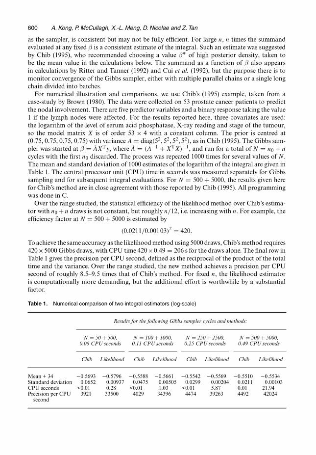
case-study by Brown (1980). The data were collected on 53 prostate cancer patients to predictthe nodal involvement. There are five predictor variables and a binary response taking the value1 if the lymph nodes were affected. For the results reported here, three covariates are used:the logarithm of the level of serum acid phosphatase, X-ray reading and stage of the tumour,so the model matrix X is of order 53 × 4 with a constant column. The prior is centred at(0.75, 0.75, 0.75, 0.75) with varianceA = diag.52, 52, 52, 52/, as in Chib (1995). The Gibbs sam-pler was started at β = AXTy, where A = .A−1 + XTX/−1, and run for a total of N = n0 + ncycles with the first n0 discarded. The process was repeated 1000 times for several values of N.The mean and standard deviation of 1000 estimates of the logarithm of the integral are given inTable 1. The central processor unit (CPU) time in seconds was measured separately for Gibbssampling and for subsequent integral evaluations. For N = 500 + 5000, the results given herefor Chib’s method are in close agreement with those reported by Chib (1995). All programmingwas done in C.Over the range studied, the statistical efficiency of the likelihood method over Chib’s estima-
tor with n0 + n draws is not constant, but roughly n=12, i.e. increasing with n. For example, theefficiency factor at N = 500 + 5000 is estimated by
.0:0211=0:00103/2 = 420:
Toachieve the same accuracy as the likelihoodmethodusing 5000 draws,Chib’smethod requires420×5000 Gibbs draws, with CPU time 420×0:49 = 206 s for the draws alone. The final row inTable 1 gives the precision per CPU second, defined as the reciprocal of the product of the totaltime and the variance. Over the range studied, the new method achieves a precision per CPUsecond of roughly 8.5–9.5 times that of Chib’s method. For fixed n, the likelihood estimatoris computationally more demanding, but the additional effort is worthwhile by a substantialfactor.
Table 1. Numerical comparison of two integral estimators (log-scale)
Results for the following Gibbs sampler cycles and methods:
N = 50 + 500, N = 100 + 1000, N = 250 + 2500, N = 500 + 5000,0.06 CPU seconds 0.11 CPU seconds 0.25 CPU seconds 0.49 CPU seconds
Chib Likelihood Chib Likelihood Chib Likelihood Chib Likelihood
Mean + 34 −0:5693 −0:5796 −0:5588 −0:5661 −0:5542 −0:5569 −0:5510 −0:5534Standard deviation 0.0652 0.00937 0.0475 0.00505 0.0299 0.00204 0.0211 0.00103CPU seconds <0.01 0.28 <0.01 1.03 <0.01 5.87 0.01 21.94Precision per CPU 3921 33500 4029 34396 4474 39263 4492 42024second

Statistical Models for Monte Carlo Integration 601
As it happens, this is one of those problems in which the likelihood estimator of µ convergesat the standard rate, but the estimate (5.1) of the integral converges at rate n−1. The bias andstandard deviation are both O.n−1/: in this example they appear to be approximately equal inmagnitude. By contrast, Chib’s estimator converges at the standard n−1=2-rate.
6. Retrospective formulation
It is possible to give a deceptively simple derivation of equation (3.5) by a retrospective argu-ment as follows. Regardless of how the design was in fact selected, we may regard the samplesize vector .n1, : : :,nk/ as the observed value of a multinomial random vector with index nand parameter vector .π1, : : :,πk/. This assumption is innocuous provided that .π1, : : :,πk/ aretreated as free parameters to be estimated from the data. Evidently, πr = nr=n is the maximumlikelihood estimate.Mimicking the argument that is frequently employed in retrospective designs, we argue as
follows.Given that the point x has been observed, what is the probability that this point was gen-erated from distributionPr rather than from one of the other distributions? A simple calculationusing Bayes’s theorem shows that the required conditional probability vector is
p.x/ = q1.x/π1=c1∑
sqs.x/πs=cs
, : : :,qk.x/πk=ck∑sqs.x/πs=cs
:
These conditional probabilities depend only on the ratios πr=cr, and not otherwise on the base-line measure µ. Conditioning on x does not eliminate the base-line measure entirely, for cr is alinear function of µ. The conditional likelihood associated with the single observation .y,x/ isthus
.πy=cy/ qy.x/∑r.πr=cr/ qr.x/
,
and the log-likelihood is
∑rnr log.πr=cr/−
n∑i=1
log{∑r.πr=cr/ qr.xi/
}: .6:1/
Once again, the observed count vector .n1, : : :,nk/ is the complete sufficient statistic, and theassociation of y-values with x-values is not informative.
Differentiation with respect to the parameter log.cr/ gives
@l
@{log.cr/} = cr @l@cr
= −nr +n∑i=1
.πr=cr/ qr.xi/∑s.πs=cs/ qs.xi/
:
By substituting the known value πr = nr=n and setting the derivative to 0, we obtain
cr =n∑i=1
qr.xi/∑sns qs.xi/=cs
, .6:2/
which is identical to equation (3.5). That is to say, the retrospective argument, previously putforward by Geyer (1994), gives exactly the right point estimator of c.The astute reader will notice that, when we substitute nr=n for πr in the retrospective likeli-
hood, the resulting function depends only on those cs for which nr > 0, and this restriction also
602 A. Kong, P. McCullagh, X.-L. Meng, D. Nicolae and Z. Tan
applies to the maximum likelihood equation (6.2). The apparent equivalence of equations (6.2)and (3.5) is thus an illusion. By contrast with the model in Section 3, the retrospective argumentdoes not lead to the conclusion that equation (6.2) is the maximum likelihood estimate of anintegral for which qr.·/ takes negative values.Even if we are willing to overlook the remarks in the preceding paragraph and to assume
that nr > 0 for each r, the objections are not easily evaded. The difficulty at this point is thatthe conditional likelihood is a function of the ratios φr = log.πr=cr/, so the vectors π and c arenot separately estimable from the conditional likelihood. It is tempting, therefore, to substitutenr=n for πr, treating this as a known prior probability. After all, who can tell how the samplesizes were chosen? However plausible this argument may sound, the resulting ‘likelihood’ doesnot give the correct covariance matrix for log.c/. The components of the negative logarithmicsecond-derivative matrix are
− @2l
@{log.cr/}@{log.cs/} =n∑i=1
δrs.πr=cr/ qr.xi/∑tnt qt.xi/=ct
−n∑i=1
.πr=cr/.πs=cs/ qr.xi/ qs.xi/
{∑tnt qt.xi/=ct}2 : .6:3/
At .π, c/, the first term is equal to the diagonal matrix nrδrs. The second term is non-negativedefinite. To put this in an alternative matrix form, write pi for the conditional probability vectorp.xi/. Then the negative second-derivative matrix shown above is
Iφ =n∑i=1.diag{pi} − pipTi / � W −WPT P W ,
using the matrix notation of Section 4.2.To see that the inverse of this matrix cannot be the correct asymptotic variance of log.c/, con-
sider the limiting case in which q1 = q2 = : : : = qk are all equal. It is then known with certaintythat c1 = : : : = ck, even in the absence of data. But, in the second-derivative matrix shownabove, all the conditional probability vectors pi are equal to .π1, : : :,πk/. The second-derivativematrix is in fact the multinomial covariance matrix with index n and probability vector π. Thegeneralized inverse of this matrix does give the correct asymptotic variances and covariancesfor contrasts of φ = log.π=c/, as the general theory requires. But it does not give the correctasymptotic variances for log.c/, or contrasts thereof.This line of argument can be partly rescued, but to do so it is necessary to show that π and c
are asymptotically independent. This is not obvious and will not be proved here, but it is a con-sequence of orthogonality of parameters in exponential family models. By standard propertiesof likelihoods, cov{log.π/− log.c/} = I−
φ asymptotically. On the presumption that π and c areasymptotically uncorrelated, we deduce that
cov{log.c/} = I−φ − cov{log.π/} = I−
φ − diag.1=nπ/+ 11T=n: .6:4/
The term 11T=n does not contribute to the variance of contrasts of log.c/ and can therefore beignored. When evaluated at .c, π/, the resulting expression.W−WPT P W/− −W−1, involvingno n×nmatrices, is identical to equation (4.2), provided that each component nr ofW is strictlypositive.
7. Conclusions
The key contribution of this paper is the formulation of Monte Carlo integration as a statisti-cal model, making explicit what information is available for use and what information is ‘outof bounds’. Given that agreement is reached on the information available, it is now possible
Statistical Models for Monte Carlo Integration 603
to say whether an estimator is or is not efficient. Likelihood methods are thus made availablenot only for parameter estimation but also for the estimation of variances and covariances forvarious simulation designs, of which importance sampling is the simplest special case. Moreinterestingly, however, three classes of submodel are identified that have substantial poten-tial for variance reduction. The associated operations are group averaging for group invariantsubmodels, linear projection for linear submodels or mixtures and Markov chain models forMarkov chain Monte Carlo schemes. To achieve worthwhile gains in efficiency, it is necessaryto exploit the structure of the problem, so it is not easy to give universally applicable advice.None-the-less, three simple examples show that efficiency factors in the range 5–10, and possiblylarger, are routinely achievable in certain types of statistical computations. We believe that suchfactors are not exceptional, particularly for Bayesian posterior calculations.It would be remiss of us to overlook the peculiar dilemma for Bayesian computation that
inevitably accompanies the methods described here. Our formulation of all Monte Carlo activ-ities is given in terms of parametric statistical models and submodels. These are fully fledgedstatistical models in the sense of the definition given by McCullagh (2002), no more or no lessartificial than any other statistical model. Given that formulation, it might seem natural toanalyse the model by using modern Bayesian methods, beginning with a prior on Θ. If weadopt the orthodox interpretation of a prior distribution as the one that summarizes theextent of what is known about the parameter, we are led to the Dirac prior on the true measure,which is almost invariably Lebesgue measure. For once, the prior is not in dispute. This choiceleads to the logically correct, but totally unsatisfactory, conclusion that the simulated data areuninformative. The posterior distribution on Θ is equal to the prior, which is unhelpful forcomputational purposes. It seems, therefore, that further progress calls for a certain degree ofpretence or pragmatism by selecting a non-informative, or at least non-degenerate, prior onΘ. Given such a prior distribution, the posterior distribution on Θ can be obtained, and theposterior moments of the required integrals computed by standard formulae. Although theseoperations are straightforward in principle, the computations are rather forbidding, so muchso that it would be impossible to complete the calculations without resorting to Monte Carlomethods! This computational black hole, an infinite regress of progressively more complicatedmodels, is an unappealing prospect, to say the least. With this in mind, it is hard to avoid theconclusion that the old-fashioned maximum likelihood estimate has much to recommend it.
Acknowledgements
The comments of four referees on an earlier draft led to substantial improvements in presenta-tion. We would like to thank Peter Bickel for pointing out the connection with biased samplingmodels, and Peter Donnelly for discussions on various points.Support for this research was provided in part by National Science Foundation grants DMS-
0071726 (for McCullagh and Tan) and DMS-0072510 (for Meng and Nicolae).
References
Albert, J. and Chib, S. (1993) Bayesian analysis of binary and polychotomous response data. J. Am. Statist. Ass.,88, 669–679.
Bishop, Y. M.M., Fienberg, S. E. and Holland, P. W. (1975)Discrete Multivariate Analyses: Theory and Practice.Cambridge: Massachusetts Institute of Technology Press.
Brown, B. W. (1980) Prediction analyses for binary data. In Biostatistics Casebook (eds R. J. Miller, B. Efron,B. W. Brown and L. E. Moses). New York: Wiley.
Chib, S. (1995) Marginal likelihood from the Gibbs output. J. Am. Statist. Ass., 90, 1313–1321.
604 A. Kong, P. McCullagh, X.-L. Meng, D. Nicolae and Z. Tan
Craiu, R. V. andMeng, X.-L. (2004)Multi-process parallel antithetic coupling for backward and forwardMarkovchain Monte Carlo. Ann. Statist., to be published.
Cui, L., Tanner, M. A., Sinha, D. and Hall, W. J. (1992) Monitoring convergence of the Gibbs sampler: furtherexperience with the Gibbs stopper. Statist. Sci., 7, 483–486.
Deming, W. E. and Stephan, F. F. (1940) On a least-squares adjustment of a sampled frequency table when theexpected marginal totals are known. Ann. Math. Statist., 11, 427–444.
DiCiccio, T. J., Kass, R. E., Raftery, A. and Wasserman, L. (1997) Computing Bayes factors by combiningsimulation and asymptotic approximations. J. Am. Statist. Ass., 92, 903–915.
Evans, M. and Swartz, T. (2000) Approximating Integrals via Monte Carlo and Deterministic Methods. Oxford:Oxford University Press.
Firth, D. and Bennett, K. E. (1998) Robust models in probability sampling. J. R. Statist. Soc. B, 60, 3–21;discussion, 41–56.
Gelman, A. andMeng, X.-L. (1991) A note on bivariate distributions that are conditionally normal.Am. Statistn,45, 125–126.
Gelman, A. and Meng, X. L. (1998) Simulating normalizing constants: from importance sampling to bridgesampling to path sampling. Statist. Sci., 13, 163–185.
Geyer, C. J. (1994) Estimating normalizing constants and reweighting mixtures in Markov chain Monte Carlo.Technical Report 568. School of Statistics, University of Minnesota, Minneapolis.
Gill, R., Vardi, Y. andWellner, J. (1988) Large sample theory of empirical distributions in biased samplingmodels.Ann. Statist., 16, 1069–1112.
Glynn, P. W. and Szechtman, R. (2000) Some new perspectives on the method of control variates. InMonte Carloand Quasi-Monte Carlo Methods (eds K.-T. Fang, F. J. Hickernell and H. Niederreiter), pp. 27–49. New York:Springer.
Hammersley, J. M. and Hanscomb, D. C. (1964)Monte Carlo Methods. London: Chapman and Hall.Hesterberg, T. (1995) Weighted average importance sampling and defensive mixture distributions. Technometrics,37, 185–194.
Horvitz, D. G. and Thompson, D. J. (1952) A generalization of sampling without replacement from a finiteuniverse. J. Am. Statist. Ass., 47, 663–683.
Lindsay, B. (1995) Mixture Models: Theory, Geometry and Applications. Hayward: Institute of MathematicalStatistics.
Liu, J. S. (2001)Monte Carlo Strategies in Scientific Computing. New York: Springer.Liu, J. S. and Sabatti, C. (2000)GeneralizedGibbs sampler andmultigridMonte Carlo for Bayesian computation.Biometrika, 87, 353–369.
MacEachern, S. N. and Peruggia,M. (2000) Importance link function estimation forMarkov ChainMonte Carlomethods. J. Comput. Graph. Statist., 9, 99–121.
Mallows, C. L. (1985) Discussion of ‘Empirical distributions in selection bias models’ by Y. Vardi. Ann. Statist.,13, 204–205.
McCullagh, P. (2002) What is a statistical model (with discussion)? Ann. Statist., 30, 1225–1310.Meng,X.-L. andWong,W.H. (1996) Simulating ratios of normalizing constants via a simple identity: a theoreticalexplanation. Statist. Sin., 6, 831–860.
Owen, A. and Zhou, Y. (2000) Safe and effective importance sampling. J. Am. Statist. Ass., 95, 135–143.Pfeffermann, D., Skinner, C. J., Holmes, D. J., Goldstein, H. and Rasbash, J. (1998) Weighting for unequalselection probabilities in multilevel models (with discussion). J. R. Statist. Soc. B, 60, 23–40; discussion, 41–56.
Ripley, B. D. (1987) Stochastic Simulation. New York: Wiley.Ritter, C. and Tanner, M. A. (1992) Facilitating the Gibbs sampler: the Gibbs stopper and the griddy-Gibbssampler. J. Am. Statist. Ass., 97, 861–868.
Rothery, P. (1982) The use of control variates in theMonte Carlo estimation of power.Appl. Statist., 31, 125–129.Vardi, Y. (1985) Empirical distributions in selection bias models. Ann. Statist., 13, 178–203.
Discussion on the paper by Kong, McCullagh, Meng, Nicolae and Tan
Michael Evans .University of Toronto/This is an interesting and stimulating paper containing some useful clarifications. The most provocativepart of the paper is the claim that treating the approximation of an integral
I =∫f.x/ µ.dx/ .1/
as a problem of statistical inference gives practically meaningful results. Although the paper does effec-tively argue this, as my discussion indicates, I still retain some doubt about the necessity of adopting thispoint of view.
In the paper we have a sequence of integrals
Discussion on the Paper by Kong, McCullagh, Meng, Nicolae and Tan 605
ci =∫qi.x/ µ.dx/,
for i = 1, : : :, r. We want to approximate the ratios ci=cj based on samples of size ni from the normalizeddensities specified by the qi .ni = 0 whenever qi takes negative values and we assume at least one ni > 0/.If only one ni is non-zero, say n1, then the estimators are given by the importance sampling estimates
(ci
cj
)=
n∑k=1
qi.xk/
w.xk/
/n∑k=1
qj.xk/
w.xk/.2/
where w = q1=c1. Note that c1 need not be known to implement equation (2). As in the general problemof importance sampling, q1 could be a bad sampler and require unrealistically large sample sizes to makethese estimates accurate. In general, it is difficult to find samplers that can be guaranteed to be good inproblems.
If we have several ni > 0, then the problem is to determine how we should combine these samples toestimate the ratios. Perhaps an obvious choice is the importance sampling estimate (2) where w is now themixture
w.x/ =r∑i=1
ni
n
qi.x/
ci: .3/
Of course there is no guarantee that this will be a good importance sampler but, more significantly, we donot know the ci and so cannot implement this directly. Still, if we put equation (3) into equation (2), weobtain a system of equations in the unknown ratios and, as the paper points out, this system can have aunique solution for the ratios. These solutions are the estimates that are discussed in the paper.
The paper justifies these estimates as maximum likelihood estimates and more importantly uses likeli-hood theory to obtain standard errors for the estimates. The above intuitive argument for the estimatesdoes not seem to lead immediately to error estimates. Onemight suspect, however, that an argument basedon the delta theorem should generate error estimates. Since I shall not provide such an argument, we mustacknowledge the accomplishment of the paper in doing this. There are still some doubts, however, aboutthe necessity for the statistical formulation and the likelihood arguments.
The group averaging that is discussed in the paper seems closely related to the use of this technique inEvans and Swartz (2000). There it is shown that, whenG is a finite group of volume preserving symmetriesof the importance sampler w, then we can replace the basic importance sampling estimate f.x/=w.x/, withx ∼ w, by fG.x/=w.x/ where
fG.x/ = 1|G|
∑g∈Gf.gx/:
This is unbiased for integral (1) and satisfies
varw
(fG
w
)= varw
(f
w
)− Ew
{(f − fG
w
)2}: .4/
This shows that the group-averaged estimator always has variance smaller than f=w. This is because fG
and w are more alike than f and w as fG and w now share the group of symmetries G. Some standardvariance reduction methods, such as antithetic variates, can be seen to be examples of this approach.
Although equation (4) seems to indicate that we always obtain an improvement with group averaging,a fairer comparison takes into account the additional function evaluations in fG=w. In that case, it wasshown in Evans and Swartz (2000) that fG=w is a true variance reducer if and only if
|G| − 1|G| varw
(f
w
)< Ew
{(f − fG
w
)2}� varw
(f
w
):
Noting that fG=w is the orthogonal projection of f=w onto the L2.w/ space of functions invariant underG, we see that we have true variance reduction if and only if the residual .f − fG/=w accounts for aproportion that is equal to .|G| − 1/=|G| of the total variation in f=w. This implies that the larger thegroup is the more stringent is the requirement for true variance reduction. Also, if this technique is to beeffective, then f and w must be very different, at least with respect to the symmetries in G, i.e. w must be
606 Discussion on the Paper by Kong, McCullagh, Meng, Nicolae and Tan
a poor importance sampler for the original problem. This leads to some reservations about the generalutility of the method.
The group averaging technique in the paper can be seen as a generalization of this as G is not requiredto be a group of symmetries of w. Rather we symmetrize both the importance sampler and the integrandso that the basic estimator is fG=wG. It may be that wG is a more effective importance sampler than w butstill we can see that the above analysis will restrict the usefulness of the method.
Although I have expressed some reservations about some aspects of the paper, overall I found it tobe thought provoking as it introduces a different way to approach the analysis of integration problemsand this leads to some interesting results. I am happy to propose the thanks and congratulations to theauthors.
Christian P. Robert .Centre de Recherche en Economie et Statistique and Universite Dauphine, Paris/Past contributions of the authors to the Monte Carlo literature, including the notion of bridge sampling,are noteworthy, and I therefore regret that this paper does not have a similar dimension for our field.Indeed, the ‘theory of Monte Carlo integration’ that is advertised in the title reduces to a formal justifica-tion of bridge sampling, via nonparametric maximum likelihood estimation, and the device of pretendingto estimate the dominating measure allows in addition for an asymptotic approximation of the MonteCarlo error through the corresponding Fisher information matrix. Although this additional level of in-terpretation of importance and bridge sampling Monte Carlo approximations (rather than estimations)of integrals is welcome, and quite exciting as a formal exercise, it seems impossible to derive a workingprinciple out of the paper.
A remark of interest related to the supposedly unknown measure is that groups can be seen as acting onthe measure rather than on the distribution. This brings much more freedom (but also the embarrassmentof wealth) in looking for group actions, since∫
Γqs.x/ dλ.x/ =
∫Γ=G
∫Gqs.gx/ dv.g/ dλ.x/ =
∫Γ=G
|G| qs.x/ dλ.x/
is satisfied for all groups G such that dλ.gx/ = dλ.x/. However, this representation also exposes theconfusion that is central to the paper between variance reduction, which is obvious by a Rao–Blackwellargument, and Monte Carlo improvement, which is unclear since the computing cost is not takeninto account. For instance, Fig. 1 analyses the example of Section 2 based on a single realization fromP1, reparameterized to [0, 1]2, where larger groups acting on [0, 1]2 bring better approximations ofcσ=c1 = 1=σ2. However, this improvement does not directly pertain to Monte Carlo integration, butrather to numerical integration (with the curse of dimensionality lurking in the background). Al-though the paper shows examples where using the group structure clearly brings substantial agree-ment, it does not shed much light on the comparison of different groups from a Monte Carlo point ofview.
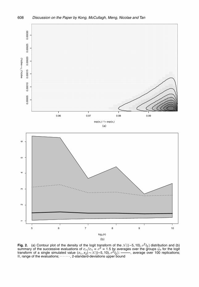
The numerical nature of the improvement is also clear when we realize that, since the group action ison the measure rather than on the distribution, it is often unlikely to be related to the geometry of thisdistribution and thus can bring little improvement when q.gxi/ = 0 for most gs and generated xis. Fig. 2shows the case of a Monte Carlo experiment on a bivariate normal distribution with the same groups asabove: the concentration of the logit transform of the N{.−5, 10/, σ2I2} distribution on a small area ofthe [0, 1]2 square (Fig. 2(a)) prevents good evaluations even after 410 computations (Fig. 2(b)).A second opening related to the likelihood representation of the weight evaluation is that a Fisher
information matrix can be associated with this problem and thus variance-like figures are produced inthe paper. Although these matrices stand as a formal ground for comparison of Monte Carlo strategies, Ihave difficulties with these figures given that they do not necessarily provide a good approximation to theMonte Carlo errors. See for instance the example of Section 2: we could apply Slutsky’s lemma with thetransform cσ = exp{log.cσ/} to obtain the variance of the cσs as
diag.cσ/V diag.cσ/,
but this approximation is invalidated by the absence of variance of the cσs. (See also the normal rangeconfidence lower bound on Fig. 2(b) which is completely unrelated to the range of the estimates.) Giventhat importance sampling estimators are quite prone to suffer from infinite variance (Robert and Casella(1999), section 3.3.2), the appeal of using Fisher information matrices is somewhat spurious as it gives afalse confidence in estimators that should not be used.

Discussion on the Paper by Kong, McCullagh, Meng, Nicolae and Tan 607
0.0 0.2 0.4 0.6 0.8 1.0
0.0
0.2
0.4
0.6
0.8
1.0
Estimate 1.44
0.0 0.2 0.4 0.6 0.8 1.0
0.0
0.2
0.4
0.6
0.8
1.0
n= 1 , Estimate 2.026
0.0 0.2 0.4 0.6 0.8 1.0
0.0
0.2
0.4
0.6
0.8
1.0
n= 2 , Estimate 2.3523
0.0 0.2 0.4 0.6 0.8 1.0
0.0
0.2
0.4
0.6
0.8
1.0
n= 3 , Estimate 2.2884
0.0 0.2 0.4 0.6 0.8 1.0
0.0
0.2
0.4
0.6
0.8
1.0
n= 4 , Estimate 2.3908
0.0 0.2 0.4 0.6 0.8 1.0
0.0
0.2
0.4
0.6
0.8
1.0
n= 5 , Estimate 2.4372
0.0 0.2 0.4 0.6 0.8 1.0
0.0
0.2
0.4
0.6
0.8
1.0
n= 6 , Estimate 2.407
0.0 0.2 0.4 0.6 0.8 1.0
0.0
0.2
0.4
0.6
0.8
1.0
n= 7 , Estimate 2.3981
0.0 0.2 0.4 0.6 0.8 1.0
0.0
0.2
0.4
0.6
0.8
1.0
n= 8 , Estimate 2.3863
Fig. 1. Successive actions of the groups Gn on the simulated value .x1, x2/ � P1 (top left-hand corner),where Gn operates on .z1, z2/ D .exp.x1/={1 C exp.x1/}, x2=.1 C x2// 2 [0, 1]2 by changing some of thefirst n bits in the binary representation of the decimal part of z1 and z2: the estimates of 1=σ2 D 2:38 aregiven above each graph; the size of the orbit of Gn is 4n
The extension to Markov chain Monte Carlo settings is another interesting point in the paper, in thatestimator (3.10) reduces to
cr =n∑t=1qr.xt/
/ n∑j=1q1.xt |xj/
if we use a single chain based on a transition q1 (with known constant). Although this estimator onlyseems to apply to the Gibbs sampler, given that the generalMetropolis–Hastings algorithm has no densityagainst the Lebesgue measure, it is a special case of Rao–Blackwellization (Gelfand and Smith, 1990;Casella and Robert, 1996) applied to importance sampling. As noted in Robert (1995), the naıve impor-tance sampling alternative
cr = 1n
n∑t=1qr.xt/=q1.xt |xt−1/,
where the ‘true’ distribution of xt is used instead, is a poor choice, since it most often suffers from infinitevariance. (The notation in Section 3.6 is mildly confusing in that cr.x/ is unrelated to cr and is also mostoften known, in contrast with cr. It thus seems inefficient to estimate the cr.xt/s.)
608 Discussion on the Paper by Kong, McCullagh, Meng, Nicolae and Tan
0.96 0.97 0.98 0.99
0.00
005
0.00
010
0.00
015
0.00
020
0.00
025
0.00
030
exp(x1) / 1 + exp(x1)
exp(
x 2)
1+
exp
(x2)
(a)
5 6 7 8 9 10
1
2
3
4
5
6
log4(n)
(b)
Fig. 2. (a) Contour plot of the density of the logit transform of the N{.�5, 10/,σ2I2} distribution and (b)summary of the successive evaluations of cσ=c1 D σ2 D 1:5 by averages over the groups Gn for the logittransform of a single simulated value .x1, x2/ � N{.�5, 10/,σ2I2}: , average over 100 replications;
, range of the evaluations; . . . . . . ., 2-standard-deviations upper bound
Discussion on the Paper by Kong, McCullagh, Meng, Nicolae and Tan 609
Except for the misplaced statements of the last paragraph about ‘orthodox Bayesians’, which simplybring to light the fundamental difference between designed Monte Carlo experiments and statistical in-ference, I enjoyed working on the authors’ paper and thus unreservedly second the vote of thanks!
The vote of thanks was passed by acclamation.
A. C. Davison .Swiss Federal Institute of Technology, Lausanne/The choice of the group is a key aspect of the variance reduction by group averaging that is suggested inthe paper, and I would like to ask its authors whether they have any advice for the bootstrapper.
The simplest form of nonparametric bootstrap entails equal probability sampling with replacementfrom data y1, : : :, yn, which is used to approximate quantities such as
m = n−1∑ t.yÅ1 , : : :, yÅn /,
where the sum is over the nn possible resamples yÅ1 , : : :, yÅn from the original data. If the statistic under
consideration is symmetric in the yj then the number of summands may be reduced to(2n−1
n
)or fewer,
but it is usually so large that m is approximated by taking a random subset of the resamples. The mostnatural group in this context arises from permuting y1, : : :, yn and has size n!, which is far too large for usein most situations. One could readily construct smaller groups, obtained for example by splitting the datainto blocks of size k and permuting within the blocks, but they seem somewhat arbitrary. How shouldthe group be chosen in this context, where the cost of function evaluations vastly outweighs the cost ofsampling?
Wenxin Jiang and Martin A. Tanner .Northwestern University, Evanston/One way to rederive equation (2.1) is to regard it as importance sampling using a sample xn1 with a ‘basedensity’ of the mixture
f.x/ =∑s
ns
n
qs.x/
cs:
The estimator of cσ = ∫Γ qσ.x/dµ would be n−1Σni=1 qσ.xi/=f.xi/. Replacing the unknown constant cs in
the base density by cs then results in a self-consistency equation that is identical to equation (2.1). (Sim-ilarly, with group averaging the functions qσ.x/ are essentially replaced by q.x;σ/ and the integrals cσ =∫
Γ q.x;σ/ dρ are estimated by using an importance sample xn1 having a base density Σs .ns=n/ q.x; s/=cs.)The goal here is to achieve a small ‘average asymptotic variance’
AAVAR =∫
Ξ
∫Ξvar{log.cσ=cτ /} dπ.σ/ dπ.τ /:
(The paper actually uses (25/20) AAVAR as the criterion function, averaging over 10 different pairs ofσ, τ ∈ Ξ = {0:25, 0:5, 1, 2, 4}:)
What is the optimal base density fo and the corresponding optimal AAVAR.fo/? The following is aresult that is obtained by applying variational calculus.
Proposition 1 (average optimality). Let cσ.f /= n−1Σni=1 qσ.xi/=f.xi/ be an estimator of cσ =∫Γ qσ.x/ dµ, where x
n1 is an independent and identically distributed sample from a probability measure
f.x/ dµ. Let
AAVAR.f / =∫
Ξ
∫Ξvar[log{cσ.f /
cτ .f /
}]dπ.σ/ dπ.τ /
for some prechosen averaging scheme defined by measure π over a set of parameters Ξ. Then
AAVAR.fo/ = inff
{AAVAR.f /} = n−1
{∫Γqo.x/ dµ.x/
}2
,
where
fo.x/ ∝ qo.x/ =√[ ∫
Ξ
∫Ξ
{qσ.x/
cσ− qτ .x/
cτ
}2
dπ.σ/ dπ.τ /]:
For the uniform–average measure π on the space Ξ = {0:25, 0:5, 1, 2, 4}, using qσ.x/ = {x21 + .x2 +σ/2}−2 and Γ = R × R+ gives (25/20) AAVAR.fo/ = 1:2=n, with the required integral computed
610 Discussion on the Paper by Kong, McCullagh, Meng, Nicolae and Tan
numerically. The paper uses the base densities f1.x/ = q1.x/=c1 and f2.x/ = Σs .1=5/ qs.x/=cs, achieving.25=20/AAVAR.f1,2/ = 3:6=n and 3:0=n, with efficiency factors AAVAR.f1,2/−1=AAVAR.fo/−1 being33% and 40% respectively, compared with the optimal fo.
It is noted that the optimal AAVAR.fo/ will be smaller if the densities {qσ.·/=cσ}σ∈Ξ are more similar.A parallel computation can be done with group averaging. Then qσ=cσ is replaced by the averaged densitypσ = 1
2 .q1=σ=c1=σ + qσ=cσ/ when computing .25=20/AAVAR.fo/, which results in a much smaller value0:20=n since the averaged densities are more similar to each other. With group averaging, the choice ofthe base density in the paper is essentially Σs .1=5/ ps.x/ ≡ f3, with .25=20/AAVAR.f3/ = 0:37=n and anefficiency factor AAVAR.f3/−1=AAVAR.fo/−1 = 54%.
The paper did not use the exact base densities f1,2,3, but rather those using the estimated normalizingconstant cs, which may have added to the variance. Nevertheless, we see that the use of group averagingseems more effective for reducing AAVAR than the use of any possible importance samples or designweights.
Hani Doss .Ohio State University, Columbus/An interesting application of the ideas in the paper arises in some current joint work with B. Narasimhan.In very general terms, our set-up is as follows. As in the usual Bayesian paradigm, we have a data vectorD, distributed according to some probability distribution Pφ, and we have a prior νh on φ. This prior isindexed by some hyperparameter h ∈ H, a subset of Euclidean space, and we are interested in νh,D, theposterior distribution of φ given the data, as h ranges over H, for doing sensitivity analyses. In our set-up,we select k values h1, : : :,hk ∈ H, and we assume that, for each r = 1, : : :, k, we have a sample φ.r/1 , : : :,φ.r/nrfrom νhr,D . We have in mind situations in which φ.r/1 , : : :,φ.r/nr are generated by Markov chain Monte Carlosampling, and in which the amount of time that it takes to generate these is non-negligible. We wish to usethe k samples to estimate νh,D, and we need to do this in realtime. (Markov chain Monte Carlo samplinggives rise to dependent samples, but to keep this discussion focused we ignore this difficulty entirely.)
In standard parametric models, the posterior is proportional to the likelihood times the prior density,i.e.
νh,D.dφ/ = c−1h lD.φ/ ν
′h.φ/ µ.dφ/,
where ch = ch.D/ is the marginal density of the data when the prior is νh, lD.φ/ is the likelihood functionand µ is a common carrier measure for all the priors. In the context of this paper, we have an infinite familyof probability distributions νh,D, h ∈ H, each known except for a normalizing constant, and we have asample from a finite number of these. The qhs may be taken to be lD.φ/ ν ′
h.φ/. The issue that for manymodels lD.φ/ is too complicated to be ‘known’ is irrelevant, since all formulae require only ratios of qs, inwhich lD cancels. Equation (3.4) gives the maximum likelihood estimate of µ, and from this we estimateνh,D.dφ/ directly via
νh,D.dφ/ = 1chqh.φ/ µ.dφ/ = 1
ch
k∑r=1
nr∑i=1
qh.φ.r/i /
k∑r=1nr qhr .φ
.r/i /=chr
δφ.r/i.dφ/
(here δa is the point mass at a), i.e. νh,D is the probability measure which gives mass
wh.i, r/ = qh.φ.r/i /=ch
k∑s=1ns qhs .φ
.r/i /=chs
={
k∑s=1nsν ′hs.φ.r/i /ch
ν ′h.φ
.r/i /chs
}−1
to φ.r/i . A potentially time-consuming computation needs to be used to solve the system of equations (3.5);however, as noted by the authors, only the system involving ch1 , : : :, chk needs to be solved, since, oncethese have been obtained, for all other hs the calculation of ch is immediate. The weights are simply thesequence {
k∑s=1ns
ν ′hs.φ.r/i /
ν ′h.φ
.r/i /chs
}−1
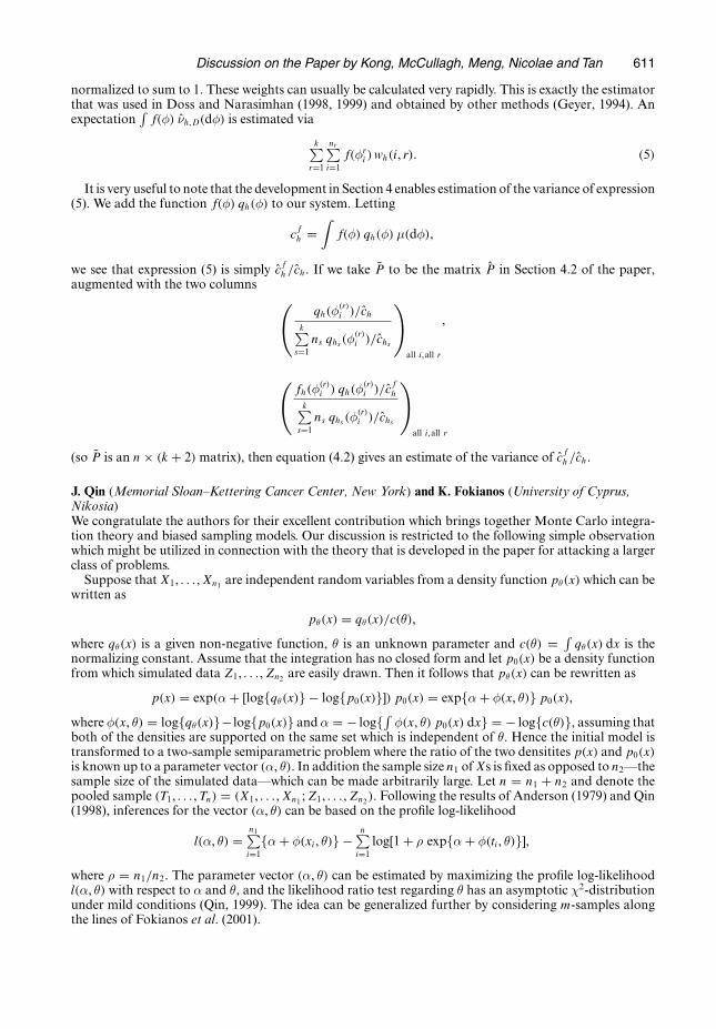
Discussion on the Paper by Kong, McCullagh, Meng, Nicolae and Tan 611
normalized to sum to 1. These weights can usually be calculated very rapidly. This is exactly the estimatorthat was used in Doss and Narasimhan (1998, 1999) and obtained by other methods (Geyer, 1994). Anexpectation
∫f.φ/ νh,D.dφ/ is estimated via
k∑r=1
nr∑i=1f.φri /wh.i, r/: .5/
It is very useful to note that the development in Section 4 enables estimation of the variance of expression(5). We add the function f.φ/ qh.φ/ to our system. Letting
cfh =
∫f.φ/ qh.φ/ µ.dφ/,
we see that expression (5) is simply cfh =ch. If we take P to be the matrix P in Section 4.2 of the paper,augmented with the two columns (
qh.φ.r/i /=ch
k∑s=1ns qhs .φ
.r/i /=chs
)all i,all r
,
(fh.φ
.r/i / qh.φ
.r/i /=c
fh
k∑s=1ns qhs .φ
.r/i /=chs
)all i,all r
(so P is an n× .k + 2/ matrix), then equation (4.2) gives an estimate of the variance of cfh =ch.
J. Qin .Memorial Sloan–Kettering Cancer Center, New York/ and K. Fokianos .University of Cyprus,Nikosia/We congratulate the authors for their excellent contribution which brings together Monte Carlo integra-tion theory and biased sampling models. Our discussion is restricted to the following simple observationwhich might be utilized in connection with the theory that is developed in the paper for attacking a largerclass of problems.
Suppose thatX1, : : :,Xn1 are independent random variables from a density function pθ.x/ which can bewritten as
pθ.x/ = qθ.x/=c.θ/,where qθ.x/ is a given non-negative function, θ is an unknown parameter and c.θ/ = ∫
qθ.x/ dx is thenormalizing constant. Assume that the integration has no closed form and let p0.x/ be a density functionfrom which simulated data Z1, : : :,Zn2 are easily drawn. Then it follows that pθ.x/ can be rewritten as
p.x/ = exp.α+ [log{qθ.x/} − log{p0.x/}]/ p0.x/ = exp{α+ φ.x, θ/} p0.x/,
where φ.x, θ/ = log{qθ.x/}− log{p0.x/} andα = − log{∫ φ.x, θ/ p0.x/ dx} = − log{c.θ/}, assuming thatboth of the densities are supported on the same set which is independent of θ. Hence the initial model istransformed to a two-sample semiparametric problem where the ratio of the two densitites p.x/ and p0.x/is known up to a parameter vector .α, θ/. In addition the sample size n1 ofXs is fixed as opposed to n2—thesample size of the simulated data—which can be made arbitrarily large. Let n = n1 + n2 and denote thepooled sample .T1, : : :, Tn/ = .X1, : : :,Xn1 ;Z1, : : :,Zn2 /. Following the results of Anderson (1979) and Qin(1998), inferences for the vector .α, θ/ can be based on the profile log-likelihood
l.α, θ/ =n1∑i=1
{α+ φ.xi, θ/} −n∑i=1
log[1 + ρ exp{α+ φ.ti, θ/}],
where ρ = n1=n2. The parameter vector .α, θ/ can be estimated by maximizing the profile log-likelihoodl.α, θ/ with respect to α and θ, and the likelihood ratio test regarding θ has an asymptotic χ2-distributionunder mild conditions (Qin, 1999). The idea can be generalized further by considering m-samples alongthe lines of Fokianos et al. (2001).
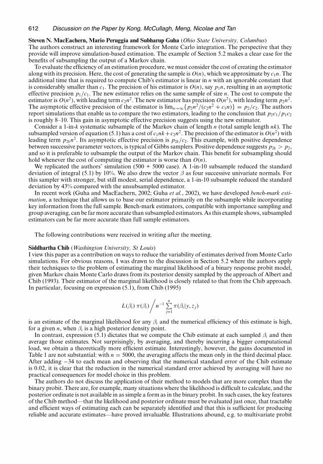
612 Discussion on the Paper by Kong, McCullagh, Meng, Nicolae and Tan
Steven N. MacEachern, Mario Peruggia and Subharup Guha .Ohio State University, Columbus/The authors construct an interesting framework for Monte Carlo integration. The perspective that theyprovide will improve simulation-based estimation. The example of Section 5.2 makes a clear case for thebenefits of subsampling the output of a Markov chain.
To evaluate the efficiency of an estimation procedure, wemust consider the cost of creating the estimatoralong with its precision. Here, the cost of generating the sample isO.n/, which we approximate by c1n. Theadditional time that is required to compute Chib’s estimator is linear in n with an ignorable constant thatis considerably smaller than c1. The precision of his estimator isO.n/, say p1n, resulting in an asymptoticeffective precision p1=c1. The new estimator relies on the same sample of size n. The cost to compute theestimator isO.n2/, with leading term c2n2. The new estimator has precisionO.n2/, with leading term p2n
2.The asymptotic effective precision of the estimator is limn→∞{p2n
2=.c2n2 + c1n/} = p2=c2. The authors
report simulations that enable us to compare the two estimators, leading to the conclusion that p2c1=p1c2is roughly 8–10. This gain in asymptotic effective precision suggests using the new estimator.
Consider a 1-in-k systematic subsample of the Markov chain of length n (total sample length nk). Thesubsampled version of equation (5.1) has a cost of c1nk+c2n2. The precision of the estimator isO.n2/withleading term p2kn
2. Its asymptotic effective precision is p2k=c2. This example, with positive dependencebetween successive parameter vectors, is typical of Gibbs samplers. Positive dependence suggests p2k > p2,and so it is preferable to subsample the output of the Markov chain. This benefit for subsampling shouldhold whenever the cost of computing the estimator is worse than O.n/.
We replicated the authors’ simulation (500 + 5000 case). A 1-in-10 subsample reduced the standarddeviation of integral (5.1) by 10%. We also drew the vector β as four successive univariate normals. Forthis sampler with stronger, but still modest, serial dependence, a 1-in-10 subsample reduced the standarddeviation by 43% compared with the unsubsampled estimator.
In recent work (Guha and MacEachern, 2002; Guha et al., 2002), we have developed bench-mark esti-mation, a technique that allows us to base our estimator primarily on the subsample while incorporatingkey information from the full sample. Bench-mark estimators, compatible with importance sampling andgroup averaging, can be farmore accurate than subsampled estimators.As this example shows, subsampledestimators can be far more accurate than full sample estimators.
The following contributions were received in writing after the meeting.
Siddhartha Chib .Washington University, St Louis/I view this paper as a contribution on ways to reduce the variability of estimates derived fromMonte Carlosimulations. For obvious reasons, I was drawn to the discussion in Section 5.2 where the authors applytheir techniques to the problem of estimating the marginal likelihood of a binary response probit model,givenMarkov chainMonte Carlo draws from its posterior density sampled by the approach of Albert andChib (1993). Their estimator of the marginal likelihood is closely related to that from the Chib approach.In particular, focusing on expression (5.1), from Chib (1995)
L.βi/ π.βi/
/n−1
n∑j=1
π.βi|y, zj/
is an estimate of the marginal likelihood for any βi and the numerical efficiency of this estimate is high,for a given n, when βi is a high posterior density point.
In contrast, expression (5.1) dictates that we compute the Chib estimate at each sampled βi and thenaverage those estimates. Not surprisingly, by averaging, and thereby incurring a bigger computationalload, we obtain a theoretically more efficient estimate. Interestingly, however, the gains documented inTable 1 are not substantial: with n = 5000, the averaging affects the mean only in the third decimal place.After adding −34 to each mean and observing that the numerical standard error of the Chib estimateis 0.02, it is clear that the reduction in the numerical standard error achieved by averaging will have nopractical consequences for model choice in this problem.
The authors do not discuss the application of their method to models that are more complex than thebinary probit. There are, for example, many situations where the likelihood is difficult to calculate, and theposterior ordinate is not available in as simple a form as in the binary probit. In such cases, the key featuresof the Chib method—that the likelihood and posterior ordinate must be evaluated just once, that tractableand efficient ways of estimating each can be separately identified and that this is sufficient for producingreliable and accurate estimates—have proved invaluable. Illustrations abound, e.g. to multivariate probit
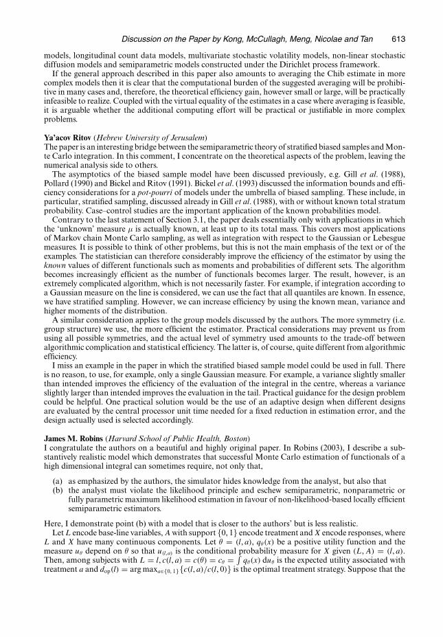
Discussion on the Paper by Kong, McCullagh, Meng, Nicolae and Tan 613
models, longitudinal count data models, multivariate stochastic volatility models, non-linear stochasticdiffusion models and semiparametric models constructed under the Dirichlet process framework.
If the general approach described in this paper also amounts to averaging the Chib estimate in morecomplex models then it is clear that the computational burden of the suggested averaging will be prohibi-tive in many cases and, therefore, the theoretical efficiency gain, however small or large, will be practicallyinfeasible to realize. Coupled with the virtual equality of the estimates in a case where averaging is feasible,it is arguable whether the additional computing effort will be practical or justifiable in more complexproblems.
Ya’acov Ritov .Hebrew University of Jerusalem/Thepaper is an interesting bridge between the semiparametric theory of stratified biased samples andMon-te Carlo integration. In this comment, I concentrate on the theoretical aspects of the problem, leaving thenumerical analysis side to others.
The asymptotics of the biased sample model have been discussed previously, e.g. Gill et al. (1988),Pollard (1990) and Bickel and Ritov (1991). Bickel et al. (1993) discussed the information bounds and effi-ciency considerations for a pot-pourri of models under the umbrella of biased sampling. These include, inparticular, stratified sampling, discussed already in Gill et al. (1988), with or without known total stratumprobability. Case–control studies are the important application of the known probabilities model.
Contrary to the last statement of Section 3.1, the paper deals essentially only with applications in whichthe ‘unknown’ measure µ is actually known, at least up to its total mass. This covers most applicationsof Markov chain Monte Carlo sampling, as well as integration with respect to the Gaussian or Lebesguemeasures. It is possible to think of other problems, but this is not the main emphasis of the text or of theexamples. The statistician can therefore considerably improve the efficiency of the estimator by using theknown values of different functionals such as moments and probabilities of different sets. The algorithmbecomes increasingly efficient as the number of functionals becomes larger. The result, however, is anextremely complicated algorithm, which is not necessarily faster. For example, if integration according toa Gaussian measure on the line is considered, we can use the fact that all quantiles are known. In essence,we have stratified sampling. However, we can increase efficiency by using the known mean, variance andhigher moments of the distribution.
A similar consideration applies to the group models discussed by the authors. The more symmetry (i.e.group structure) we use, the more efficient the estimator. Practical considerations may prevent us fromusing all possible symmetries, and the actual level of symmetry used amounts to the trade-off betweenalgorithmic complication and statistical efficiency. The latter is, of course, quite different from algorithmicefficiency.
I miss an example in the paper in which the stratified biased sample model could be used in full. Thereis no reason, to use, for example, only a single Gaussian measure. For example, a variance slightly smallerthan intended improves the efficiency of the evaluation of the integral in the centre, whereas a varianceslightly larger than intended improves the evaluation in the tail. Practical guidance for the design problemcould be helpful. One practical solution would be the use of an adaptive design when different designsare evaluated by the central processor unit time needed for a fixed reduction in estimation error, and thedesign actually used is selected accordingly.
James M. Robins .Harvard School of Public Health, Boston/I congratulate the authors on a beautiful and highly original paper. In Robins (2003), I describe a sub-stantively realistic model which demonstrates that successful Monte Carlo estimation of functionals of ahigh dimensional integral can sometimes require, not only that,
(a) as emphasized by the authors, the simulator hides knowledge from the analyst, but also that(b) the analyst must violate the likelihood principle and eschew semiparametric, nonparametric or
fully parametric maximum likelihood estimation in favour of non-likelihood-based locally efficientsemiparametric estimators.
Here, I demonstrate point (b) with a model that is closer to the authors’ but is less realistic.LetL encode base-line variables,Awith support {0, 1} encode treatment andX encode responses, where
L and X have many continuous components. Let θ = .l, a/, qθ.x/ be a positive utility function and themeasure uθ depend on θ so that u.l,a/ is the conditional probability measure for X given .L,A/ = .l, a/.Then, among subjects with L = l, c.l, a/ = c.θ/ = cθ = ∫ qθ.x/ duθ is the expected utility associated withtreatment a and dop.l/ = argmaxa∈{0, 1}{c.l, a/=c.l, 0/} is the optimal treatment strategy. Suppose that the
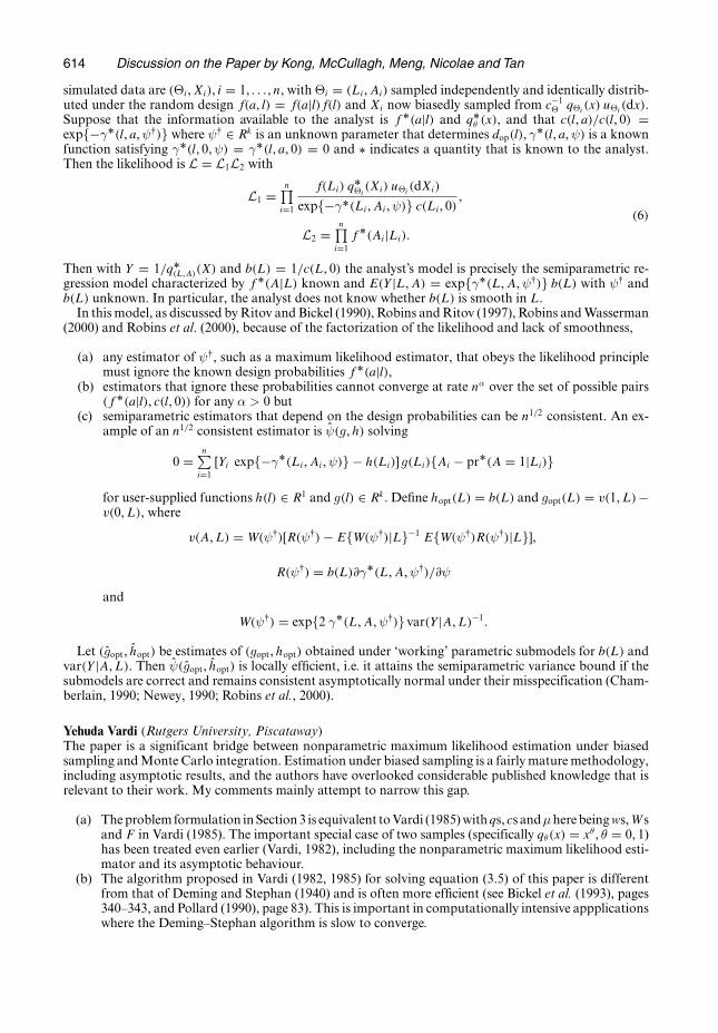
614 Discussion on the Paper by Kong, McCullagh, Meng, Nicolae and Tan
simulated data are .Θi,Xi/, i = 1, : : :, n, with Θi = .Li,Ai/ sampled independently and identically distrib-uted under the random design f.a, l/ = f.a|l/f.l/ and Xi now biasedly sampled from c−1
Θ qΘi .x/ uΘi .dx/.Suppose that the information available to the analyst is fÅ.a|l/ and qÅθ .x/, and that c.l, a/=c.l, 0/ =exp{−γÅ.l, a,ψ†/} where ψ† ∈ Rk is an unknown parameter that determines dop.l/, γÅ.l, a,ψ/ is a knownfunction satisfying γÅ.l, 0,ψ/ = γÅ.l, a, 0/ = 0 and Å indicates a quantity that is known to the analyst.Then the likelihood is L = L1L2 with
L1 =n∏i=1
f.Li/ qÅΘi .Xi/ uΘi .dXi/
exp{−γÅ.Li,Ai,ψ/} c.Li, 0/ ,
L2 =n∏i=1fÅ.Ai|Li/:
.6/
Then with Y = 1=qÅ.L,A/.X/ and b.L/ = 1=c.L, 0/ the analyst’s model is precisely the semiparametric re-gression model characterized by fÅ.A|L/ known and E.Y |L,A/ = exp{γÅ.L,A,ψ†/} b.L/ with ψ† andb.L/ unknown. In particular, the analyst does not know whether b.L/ is smooth in L.
In this model, as discussed byRitov and Bickel (1990), Robins andRitov (1997), Robins andWasserman(2000) and Robins et al. (2000), because of the factorization of the likelihood and lack of smoothness,
(a) any estimator of ψ†, such as a maximum likelihood estimator, that obeys the likelihood principlemust ignore the known design probabilities fÅ.a|l/,
(b) estimators that ignore these probabilities cannot converge at rate nα over the set of possible pairs.fÅ.a|l/, c.l, 0// for any α > 0 but
(c) semiparametric estimators that depend on the design probabilities can be n1=2 consistent. An ex-ample of an n1=2 consistent estimator is ψ.g,h/ solving
0 =n∑i=1
[Yi exp{−γÅ.Li,Ai,ψ/} − h.Li/] g.Li/{Ai − prÅ.A = 1|Li/}
for user-supplied functions h.l/ ∈ R1 and g.l/ ∈ Rk. Define hopt.L/ = b.L/ and gopt.L/ = v.1,L/−v.0,L/, where
v.A,L/ = W.ψ†/[R.ψ†/− E{W.ψ†/|L}−1 E{W.ψ†/R.ψ†/|L}],
R.ψ†/ = b.L/@γÅ.L,A,ψ†/=@ψ
and
W.ψ†/ = exp{2 γÅ.L,A,ψ†/}var.Y |A,L/−1:
Let .gopt, hopt/ be estimates of .gopt,hopt/ obtained under ‘working’ parametric submodels for b.L/ andvar.Y |A,L/. Then ψ.gopt, hopt/ is locally efficient, i.e. it attains the semiparametric variance bound if thesubmodels are correct and remains consistent asymptotically normal under their misspecification (Cham-berlain, 1990; Newey, 1990; Robins et al., 2000).
Yehuda Vardi .Rutgers University, Piscataway/The paper is a significant bridge between nonparametric maximum likelihood estimation under biasedsampling andMonte Carlo integration. Estimation under biased sampling is a fairlymaturemethodology,including asymptotic results, and the authors have overlooked considerable published knowledge that isrelevant to their work. My comments mainly attempt to narrow this gap.
(a) Theproblem formulation inSection3 is equivalent toVardi (1985)withqs, cs andµherebeingws,Wsand F in Vardi (1985). The important special case of two samples (specifically qθ.x/ = xθ, θ = 0, 1)has been treated even earlier (Vardi, 1982), including the nonparametric maximum likelihood esti-mator and its asymptotic behaviour.
(b) The algorithm proposed in Vardi (1982, 1985) for solving equation (3.5) of this paper is differentfrom that of Deming and Stephan (1940) and is often more efficient (see Bickel et al. (1993), pages340–343, and Pollard (1990), page 83). This is important in computationally intensive appplicationswhere the Deming–Stephan algorithm is slow to converge.
Discussion on the Paper by Kong, McCullagh, Meng, Nicolae and Tan 615
(c) Regarding the asymptotics, for two samples, equation (4.2) should match theorem 3.1 of Vardi(1982) and it would be constructive to show this. For more than two samples, equation (4.2) shouldmatch proposition 2.3 in Gill et al. (1988) and similar results in Bickel et al. (1993).
(d) More on the asymptotics: ‘lifting’ the limiting behaviour of the estimated crs from standard proper-ties of the exponential family, although a useful shortcut, seems mathematically heuristic. A gooddiscussion of the interplay between the parametric and nonparametric aspects of the model is inchapter 14 of Pollard (1990).
(e) The methodology calls for generating samples from weighted distributions, but this is often a diffi-cult problemwith no satisfactory solution, so there is a computational trade-off here. Note problem6.1 of Gill et al. (1988), which also connects biased sampling methodology with design issues andimportance sampling.
(f) Gilbert et al. (1999) extended the model to include weight functions qrs, which share a commonunknown parameter. This might be useful in future applications of your methodology.
(g) You allow negative qrs but assume zero observations for such samples (nr = 0 in the discussionfollowing equation (3.1)). This is confusing. A simple example with negative weight function(s) andan explanation of how to estimate the ratio of integrals in this case would help.
(h) Woodroofe (1985) showed that the nonparametric maximum likelihood estimator from truncateddata is consistent only under certain conditions on the probabilities that generate the data. Wood-roofe’s problem has a similar data structure to yourMarkov chainmodels of Section 3.6, where eachtargeted distribution has a sample of size 1 or less. This leads me to think that further conditionsmight be necessary to achieve consistency.
The authors replied later, in writing, as follows.
General remarksThe view presented in the paper is that essentially every Monte Carlo activity may be interpreted asparameter estimation by maximum likelihood in a statistical model. We do not claim that this point ofview is necessary; nor do we seek to establish a working principle from it. By analogy, the geometricinterpretation of linear models is not necessary for fitting or understanding; nor is there a geometric work-ing principle. The fact that the estimators are obtained by maximum likelihood does not mean that theycannot be justified or derived by heuristic arguments, even by flawed arguments. The crux of the matter isnot necessity or working principle, but whether the new interpretation is helpful or useful in the sense ofleading to new understanding, better simulation designs or more efficient algorithms. Jiang and Tanner’soptimal sampler, although not readily computable and not from themixture class, is a step in this direction.The remark by MacEachern, Peruggia and Guha is another step showing that, for slow mixing Markovchains, the numerical efficiency of superefficient estimators, such as those described in Section 5.2, maybe improved by subsampling.
Several discussants (Evans, Robert, Davison, : : :) raise questions about group averaging, its effective-ness, how to choose the group, and so on. As Robert correctly points out, having the group act on theparameter space rather than on the sampler provides great latitude for choice of group actions. Groupaveraging can be very effective with a small group or very ineffective with a large group, the latter beingcounter-productive. The group actions that we have in mind involve very small groups, so the additionalcomputational effort is small, if not quite negligible. To choose an effective group action, it is usuallynecessary to take advantage of the structure of the problem, the symmetries or geometry of the modelor the topology of the space. Euclidean spaces have ample structure for interesting group actions. Theparameter space in a parametric mixture model has obvious symmetries that can potentially be exploited.In the nonparametric bootstrap, unfortunately, these useful pieces of structure have been stripped away,the space that remains being a forlorn finite set with no redeeming structure. In the examples that we haveexplored, effective group action carries each sample point to a different point that is not usually in thesample. The bootstrap restriction to the observed sample points precludes group actions other than finitepermutations. If the retention of structure is not contrary to bootstrap principles, it may be possible touse temporal order, or factor levels or covariate values, and to permute the covariates or the design. Ofcourse, this may be precisely what you do not want to do.
It is true, as Ritov points out, that maximum likelihood becomes more efficient as the parameter spaceis reduced by the inclusion of symmetries or additional information such as the values of certain integrals.Our submodels are designed to exploit exactly that. The hard part of the exercise is to construct a submodelsuch that the gain in precision is sufficient to justify the additional computational effort. Evans’s remarks
616 Discussion on the Paper by Kong, McCullagh, Meng, Nicolae and Tan
show that the potential gain from the traditional type of group action is very limited. We doubt that it ispossible to put a similar bound on the effectiveness of the group action on the parameter space.
Mixtures versus strataRemarks by Evans and Jiang and Tanner suggest that it may be helpful to explain why four superficiallysimilar estimators can have very different variances:
(a) the biased sampling estimator or bridge sampling estimator (BSE);(b) the importance sampling estimator in which a single sample is drawn from the mixture;(c) the post-stratified importance sampling estimator with actual sample sizes as weights;(d) the stratified estimator in which the relative normalizing constants for the samplers are given.
We have listed these in increasing order of available information. The principal distinction is that theBSE does not use the normalizing constants for the samplers. The fourth estimator is maximum likelihoodsubject to certain homogeneous linear constraints of the type described in Section 3.4. For (a)–(c), theestimated mass at the sample point xi is
dµ.xi/ ∝ n∑s
ns qs.xi/=cs,
dµ.xi/ ∝ 1∑s
πs qs.xi/=cs
and
dµ.xi/ ∝ n∑s
ns qs.xi/=cs:
For (d) with the restriction c1 = : : : = ck, the estimator obtained by constrained maximization over theset of measures supported on the data is
dµ.xi/ ∝ 1∑λr qr.xi/
,
the ratios λr=λs being determined by the condition cr = cs, where cr = ∫qr dµ. The constrained max-
imum likelihood estimator is in a mixture form even though there may be draws from only one of thedistributions.
Two designs with Γ = [0, 2] show that the variances are not necessarily comparable:
q1.x/ = I.0 � x � 1/; q2.x/ = I.1 � x � 2/; n1 = 2n2 .design I/;
q1.x/ = 0:5 I.0 � x � 2/; q2.x/ = I.0 � x � 1/; n1 = 2n2 .design II/;
plus the mixture with weights . 23 ,13 /. The absence of an overlap between q1 and q2 in design I means that
µ is not estimable. The BSE of an integral such that the integrand is non-zero on both intervals does notexist. In practical terms, the variance is infinite. However, the restriction of µ to each interval is estimable,and the additional information that c1 = c2 means that these estimated measures can be combined insuch a way that µ.[0, 1]/ = µ.[1, 2]/. The stratified maximum likelihood estimator (d) puts mass 1 at eachsample point in the first interval and 2 at each point in the second. In an importance sampling design withindependent and identically distributed observations from the mixture, the estimator (b) has the sameform with weights 1 or 2 at each sample point. But the number of observations falling in each intervalis binomial, so the measure does not have equal mass on the two intervals. This defect is corrected by apost-stratification adjustment. Estimator (d) has the natural property that, for each function q3 that is alinear combination of q1 and q2, the ratio c3=c1 has zero variance even if the draws come entirely from P2.Themain point of this example is that, although the formulae in all cases look likemixture sampling, the
estimators can have very different variances. As Jiang and Tanner note, the use of estimated normalizingconstants in the BSE may increase the variance, potentially by a large factor. Also, their optimal sampleris not in the mixture family, so the comparison is not entirely fair.
VariancesVardi makes the point that, for a given sequence of designs, only certain integrals are consistently esti-mable. It would be good to have a clean description of this class, how it depends on the design and on
Discussion on the Paper by Kong, McCullagh, Meng, Nicolae and Tan 617
the group action. The asymptotic variance estimates reported in the paper are in agreement with knownresults such as proposition 2.3 in Gill et al. (1988), but they apply only to integrals that are consistentlyestimable. Our experience has been that the Fisher information calculation usually matches up well withempirical simulation variances. At the same time, we have not looked at extreme cases near the boundaryof the consistently estimable class, where the approximation might begin to break down. Robert’s examplewith n = 1 sheds little light on the adequacy of the asymptotic variance formulae. In applications of thissort, where the log-ratios log(cr=cs) do not havemoments, the distinction between variance and asymptoticvariance is critical. The asymptotic variance is well defined and finite, and this is the relevant number forthe assessment of precision in large samples.
Retrospective, empirical and profile likelihoodThe simplest way to phrase the remarks by Qin and Fokianos is to consider a regression model withresponse Y and covariate x in which the components of Y are independent with distribution
qθ.y/ dµ.y/=cθ.µ/
where θi = xiβ, and µ is an arbitrary measure. The likelihood maximized over µ for fixed β is a func-tion of β alone, here assumed to be a scalar. If the covariate is binary, as in a two-sample problem, thetwo-parameter function given by Qin and Fokianos is such that l.αβ ,β/ is the profile log-likelihood for β.An equivalent result can be obtained by a conditional retrospective argument along the lines of Armitage(1971). In particular, if log{qθ.y/} is linear in θ, both arguments lead to a likelihood constructed as if theconditional distribution given y satisfies a linear logistic model with independent components.
Comparisons of precisionTable 1 shows that the precision previously achieved in nine times units can now be achieved in one timeunit. Professor Chib argues unconvincingly that this is not a substantial factor. Possibly he has too muchtime on his hands. His subsequent remark about the addition of −34 to each value in Table 1 can only beinterpreted tongue in cheek, so the comment about insubstantial factors may be meant likewise.
Likelihood principleAlthough it appears to have no direct bearing on any of our results, Robins’s example raises interestingfundamental issues connected with the likelihood function, its definition and its interpretation. As weunderstand it, the likelihood principle does not address matters connected with asymptotics; nor doesit promote point estimation as an inferential activity. In particular, the non-existence of a maximum orsupremum is not regarded as a contradiction of the likelihood principle; nor is the existence of multiplemaxima. By convention, an estimator is said to ‘obey the likelihood principle’ if it is a function of thesufficient statistic.
In writing this paper, we had given no thought to the applicability of the likelihood principle in infinitedimensional models. On reflection, however, it is essential that likelihood ratios be well defined, and, toachieve this, topological conditions are unavoidable. Such conditions are natural in statistical work be-cause an observation is a point in a topological space, in which the σ-field is generated by the open sets.Time and space limitations preclude more detailed discussion, but an example in which Θ is the set ofLebesgue measurable functions [0, 1] → [0, 1] illustrates one aspect of the matter. If the model is such thatYi is Bernoulli with parameter θ.xi/, the ‘likelihood’ expression
L.θ/ =∏ θ.xi/yi{1 − θ.xi/}1−yi
is not a function on Θ as a topological space. Two functions θ and θ′ differing on a null set represent thesame point in the topological space Θ, but they may not have the same ‘likelihood’. In other words, θ = θ′
does not imply L.θ/ = L.θ′/, so L is not a function on Θ. None-the-less, there are non-trivial submodelsfor which the likelihood exists and factors, and the Robins phenomenon persists.
References in the discussion
Albert, J. and Chib, S. (1993) Bayesian analysis of binary and polychotomous response data. J. Am. Statist. Ass.,88, 669–679.
Anderson, J. A. (1979) Multivariate logistic compounds. Biometrika, 66, 17–26.Armitage, P. (1971) Statistical Methods in Medical Research. Oxford: Blackwell.Bickel, P. J., Klaassen, C. A. J., Ritov, Y. andWellner, J. A. (1993) Efficient and Adaptive Estimation for Semipara-metric Models. Baltimore: Johns Hopkins.
618 Discussion on the Paper by Kong, McCullagh, Meng, Nicolae and Tan
Bickel, P. J. and Ritov, Y. (1991) Large sample theory of estimation in biased sampling regression, model I. Ann.Statist., 19, 797–816.
Casella, G. and Robert, C. P. (1996) Rao-Blackwellisation of sampling schemes. Biometrika, 83, 81–94.Chamberlain, G. (1988) Efficiency bounds for semiparametric regression. Technical Report. Department of Eco-nomics, University of Wisconsin, Madison.
Chib, S. (1995) Marginal likelihood from the Gibbs output. J. Am. Statist. Ass., 90, 1313–1321.Deming, W. E. and Stephan, F. F. (1940) On a least-squares adjustment of a sampled frequency table when theexpected marginal totals are known. Ann. Math. Statist., 11, 427–444.
Doss, H. and Narasimhan, B. (1998) Dynamic display of changing posterior in Bayesian survival analysis.In Practical Nonparametric and Semiparametric Bayesian Statistics (eds D. Dey, P. Muller and D. Sinha),pp. 63–87. New York: Springer.
Doss, H. and Narasimhan, B. (1999) Dynamic display of changing posterior in Bayesian survival analysis: thesoftware. J. Statist. Softwr., 4, 1–72.
Evans, M. and Swartz, T. (2000) Approximating Integrals via Monte Carlo and Deterministic Methods. Oxford:Oxford University Press.
Fokianos, K., Kedem, B., Qin, J. and Short, D. A. (2001) A semiparametric approach to the one-way layout.Technometrics, 43, 56–65.
Gelfand, A. E. and Smith, A. F. M. (1990) Sampling based approaches to calculating marginal densities. J. Am.Statist. Ass., 85, 398–409.
Geyer, C. J. (1994) Estimating normalizing constants and reweighting mixtures in Markov chain Monte Carlo.Technical Report 568. School of Statistics, University of Minnesota, Minneapolis.
Gilbert, P. B., Lele, S. R. and Vardi, Y. (1999) Maximum likelihood estimation in semiparametric selection biasmodels with application to AIDS vaccine trials. Biometrika, 86, 27–43.
Gill, R., Vardi, Y. andWellner, J. (1988) Large sample theory of empirical distributions in biased samplingmodels.Ann. Statist., 16, 1069–1112.
Guha, S. and MacEachern, S. N. (2002) Benchmark estimation and importance sampling with Markov chainMonte Carlo samplers. Technical Report. Ohio State University, Columbus.
Guha, S., MacEachern, S. N. and Peruggia, M. (2002) Benchmark estimation for Markov chain Monte Carlosamples. J. Comput. Graph. Statist., to be published.
Newey, W. (1990) Semiparametric efficiency bounds. J. Appl. Econometr., 5, 99–135.Pollard, D. (1990) Empirical Processes: Theory and Applications. Hayward: Institute of Mathematical Statistics.Qin, J. (1998) Inferences for case-control and semiparametric two-sample density ratio models. Biometrika, 85,619–630.
Qin, J. (1999) Case-control studies and Monte Carlo methods. Unpublished.Ritov, Y. and Bickel, P. (1990) Achieving information bounds in non- and semi-parametric models. Ann. Statist.,18, 925–938.
Robert, C. P. (1995) Convergence control techniques for MCMC algorithms. Statist. Sci., 10, 231–253.Robert, C. P. and Casella, G. (1999)Monte Carlo Statistical Methods. New York: Springer.Robins, J. M. (2003) Estimation of optimal treatment strategies. In Proc. 2nd Seattle Symp. Biostatistics, to bepublished.
Robins, J. M. and Ritov, Y. (1997) A curse of dimensionality appropriate (CODA) asymptotic theory for semi-parametric models. Statist. Med., 16, 285–319.
Robins, J. M., Rotnizky, A. and van der Laan, M. (2000) Comment on ‘On profile likelihood’ (by S. A. Murphyand A. W. van der Vaart). J. Am. Statist. Ass., 95, 431–435.
Robins, J. M. andWasserman, L. (2000) Conditioning, likelihood, and coherence: a review of some foundationalconcepts. J. Am. Statist. Ass., 95, 1340–1346.
Vardi, Y. (1982) Nonparametric estimation in the presence of length bias. Ann. Statist., 10, 616–620.Vardi, Y. (1985) Empirical distributions in selection bias models. Ann. Statist., 13, 178–203.Woodroofe, M. (1985) Estimating a distribution function with truncated data. Ann. Statist., 13, 163.