A theoretical study of two-color photoionization and autoionization of molecules

Journal ofPhotochemistry, .39 (1987) 173 - 200 173

A TJ3EORETlCAL STUDY OF TWO-COLOR PHOTOIONIZATION AND AUTOIONIZATION OF MOLECULES

S. H. LIN and A. B0EGLJ.N

Department of Chemiefry, Arizona St&e Uniuereity, Tempe,

s. M. LIN

InsMute uf Atomic and Mokcukr Science. Academia Sinica

(Received January 22,1987)

AZ 8628 7 (US.A,)

(Taiwan)

The main purpose of this paper is to apply the density matrix formalism for treating multiphoton ionization of multirovibronic level systems. Both direct photoionization and photoionixation through autoionization states are taken into account. Numerical results will be presented fordemonstrating the effect of the interference resulting from the’ neighboring rovibronic levels. The theoretical results are applied to interpret two sets of experimental data on two-color photoionixation of molecules; one set is for two- color threshold photoionization spectra of jet-cooled aniline which exhibit autoionizing Rydberg structures and the other is for high resolution Rydberg spectra of Hz by stepwise resonance two-photon ion-pair (H+ + H-) production.

1. Introduction

Two-color photoionization studies have provided important insights into studies of the properties of highly excited states of molecules, such as the precise determination of ionization energies and lifetimes of excited states, the de-ion of autoionizing states and the investigation of photo- fragmentation phenomena El]. By using resonant two-photon excitation, the weak transition probabilities due to small Franck-Condon factors for single-photon excitation can be greatly improved. New excited states whose transitions cannot be easily reached from the ground state can be studied. For small molecules, the spectrum can also be simplified by selective labelling of the rotational states.

In previous papers [2,3], we have developed a density matrix formalism for treating one-photon ionization and two-photon ionization of molecules. We have shown that Fano’s results [4] for one-photon autoionization can be reproduced by this formalism. It has also been shown that this density matrix method can treat two-color photoionization spectroscopy and the

0047-2670/87/$3&O 0 Elsevier Sequoia/Printed in The Netherlands

174

measurement of excited state lifetimes by the multiphoton ionization tech- nique.

In this paper, we shall extend this density matrix method to take into account the multilevel effect on one-photon and two-photon ionization of molecules and apply the theoretical results to the analysis of some recent experimental data. It should be noted that in our previous papers [Z, 31 for one-photon ionization we considered only two discrete levels and for two- photon ionization we considered only three discrete levels. In this paper, the effect of the existence of multirovibronic levels in the ground and excited electronic states is taken into account.

2. Theory

It has been shown that the master equations (MEs) for the photoionization of molecules in the Markoff approximation can be expressed as c2931

%an * - + ; ~uiAwd&n- at Pnmv,,) + c ErPmm+ c CRiiE%nm~ = 0

m m m ??I’

and

ap?nn at

+ (iti, + lTE)p- f ; 5 (V_#P??aJ” - J&nm#Vm,)

+ cc R&+P~I~I = 0 m’ n’

where

R 2 = &nJ_e f &_, J&a

=$zj

f

J ?nn’ dr V,(t)Vcml(t -T) exp -i s da, ~crn’(tl) CO f--r

and f=fi+O

(2-l)

(2-2)

(2-3)

(2-4)

(2-5) Here if represents the perturbation for inducing autoionization and fi denotes the interaction hamiltonian between the system and the radiation field. In eqns. (2-1) and (2-2), the I’M are the relaxation rate constants and r= represents the depbasing rate constant. In eqn. (2-4), the summation over c refers to the continuum states above the ionization threshold.

For convenience, we shall present the theoretical treatment of one- photon ionization and two-photon ionization of multilevel systems separately.

175

2.1. One-photon ionization we shall let n denote a vibronic (or a rovibronic) level in the ground

electronic state g and m represent a vibronic (or a rovibronic) level in the excited electronic state a (we Fig. 1). The MEs in this mse are

%nn at

~rm.KwJ + RE%m + RE’P,,

+RE~,.,+~r~p,=0 k

and

aPmn at

+ (iw, +rm”+Rz)p_+ $cin(pnn-~)

+Rzp,,,,+R”h=Q

(2-6)

(2-V

where ZkrM’$&plrk and &l-‘zpkk include both electronic relaxation and vibrational relaxation. For convenience we shall ignore the inverse electronic relaxation.

I / I / I /

n I /

9

Fig. 1. One-photon ionization.

176

Applying the steady state approximation to eqn. (2-8) yields (Appen- dixA)

ap?l?l - + (R at “,E +A,)p, + C A-p,, + c rF& + 2 %“hrw = 0 (2-9) m m n’

ham at + (R”” +A,,,,,,)&,,,, + ~Ampnn+~I-~'pm~m~ - zl--Ep- = 0

n m’ n

(2-10)

where the FE represent electronic relaxation rate constants, while Fe’; FI’“’ etc. denote vibrational relaxation constants. Other quantities in eqns.

&!%I and (2-10) are defined as follows:

il~~lfi1-~)19m>l*(1 -ii/ad2 i(o,---uw)+r~+R~

(2-11)

&=A_=-+ il(?Zll3(--0)1@~)1*(1+ 1/qm2) i(o,-GJ)+r~+R~ t

(2-12)

A i l~~ml15~w)ln>12~1 + ikd2

mm =$zlm\ i(o_-u)+rz+RE 1 (2-13) ”

and

In this case, the photoionization yield Y(t) is given by

(2-14)

(2-15)

ah Y(t) = - c - -

n at ga+ = Zi R~++A,+~&rm

n m )~,,n+~(RLZE+&m+~h.m)~mm (2-W

The integrated yield (or efficiency) is defined by

W)=1-_CP?m- CP- n m

(2-16A)

177

In the weak intensity and short time regime, we can ignore the excited state distributions p,,,,,,

Y=CRZ--& n [

(l/hdWk - 0) + W~m2WCXr) + CKXr)l

m Mwl - w)" + Cl?=(r) + R”(rjj2

X I(~l~(W)I&n)12 I

Pm (Z-17)

where FE(r) and R=(r) represent the real parts of I’= and RE respectively, and determine the bandwidth of Y ~0. w; the imaginary portions of FE and Rz which determine the band shift of Y vs. w have been included in wk (see Appendix A).

For the weak field case, if we can apply the steady state approximation to JI,- given by eqn. (2-lo), then substituting the resulting p,_ into eqn. (2-16) we obtain

(2-17A)

where w_ = -x,rr represents the electronic relaxation of the mth level. Here the vibrational relaxation terms &,Jm~'pmlm~ have been ignored; this approxikation is valid only when the vibrational relaxation is very slow or when the vibrational equilibrium is established. When W,, * R; eqn. (2-17A) reduces to eqn. (2-17) and when W,, Q Rz eqn. (2-17A) reduces to

Y= ~W~+&nhn (247B) n

which exhibits the Fano-type bandshape (cf. eqn. (2-20)). According to the theoretical analysis of the two-discrete-level model of

one-photon ionization of molecules, for the weak-field case, and in the short time region 133, the approximate expression for Y given by eqn. (2-17) is more accurate then that given by eqn. (2-17A).

Notice that Rg and RE denote the direct photoionixation rate and the autoionization rate respectively, that is

RM= nn

and

R-z mm

(2-18)

Equation (2-17) shows that the photoionization yield consists of two parts, the contribution from the direct photoionization Rz and the contribution through autoionization A, + ZmA, (or A, if eqn. (2-17B) is valid). The

178

latter contribution gives us the Beutler-Fano asymmetric bandshape of photoionization. From eqn. (2-g), we can see that the rate constant

K,,=R”,“+A, (2-9A) represents the depletion rate of the nth level of the ground electronic state through the ionization channel, and again K,, consists of the contributions from the direct photoionization and fiorn autoionization A,. Notice that A, can be rewritten as

A fi: c (1 - uLm2 )CCXr) + REXr)l - (2hrdWk - W =- nn

bL?l- w)’ + {I’z(r) + R=(r)}2

x I~nllS(-Wlha~12 (2-1sA)

where w&, = o, + Rz (i) + l? E(i). Defining the detuning

(2-113)

eqn. (2-1lA) becomes

Notice that (am2 - 1 + 2q,e,,)/(l+ E,~) is the lineshape expression derived by Fano 141. However, the physical meanings of Fano’s expression and ours are somewhat different. In Fano’s case, the spectral linewidth is due to autoionization only while in our case the spectral linewidth consists of the contribution from the lifetimes of the n-level and the m-level and pure dephasing through r=(r) and the contribution from the rates of direct photoionixation and autoionixation through Rz (r).

2.2. Two-photon ionization Figure 2 shows the energy level scheme for two-color two-photon

ionization of molecules. That is, we let I, n and m represent the rovibronic (or vibronic) levels of the ground electronic state, first excited state and second excited state respectively. The equations of motion for the diagonal elements prz, A, and hrn are given by

(2-21)

(2-22)

179

m A m .

Fig. 2. Two-color, two-photon ionization.

+~r”_p*=o k

(2-23)

Using eqns. (2-3) - (2-5) and eqn. (A-2) of Appendix A, eqns. (2-21) - (2-23) become

and

(2-25)

(2-26)

180

where

I#,>= Im>+ (2-27)

(2-28)

a:,= w3(-~2~21 J/,1

(m/R) ~D~(-w2)2 ucms(w* - WC” 1 (2-29)

c

and

Qnm =, (4a--2)2I$m)

(a/h) C Dnc(--w2)2ucms(0cm) (2-30)

c

The c&rivation of eqns. (2-24) - (2-26) is similar to that for the one-photon ionization case given in Appendix A.

Next we consider the equations of motion for the off-diagonal density matrix elements

(2-31)

ak-k .

at + (iw, +rE+Rm”)hr,+ f Km(Pnn -f&am) .

-_~Pm’V;“+(R~~+R~P~)=O

These expressions can be simplif‘ied (see Appendix B) as

ahh.d .

at + IiWd - WI) + r:: + R”,:hd~~) +

(2-33)

--PM)

(2-34)

181

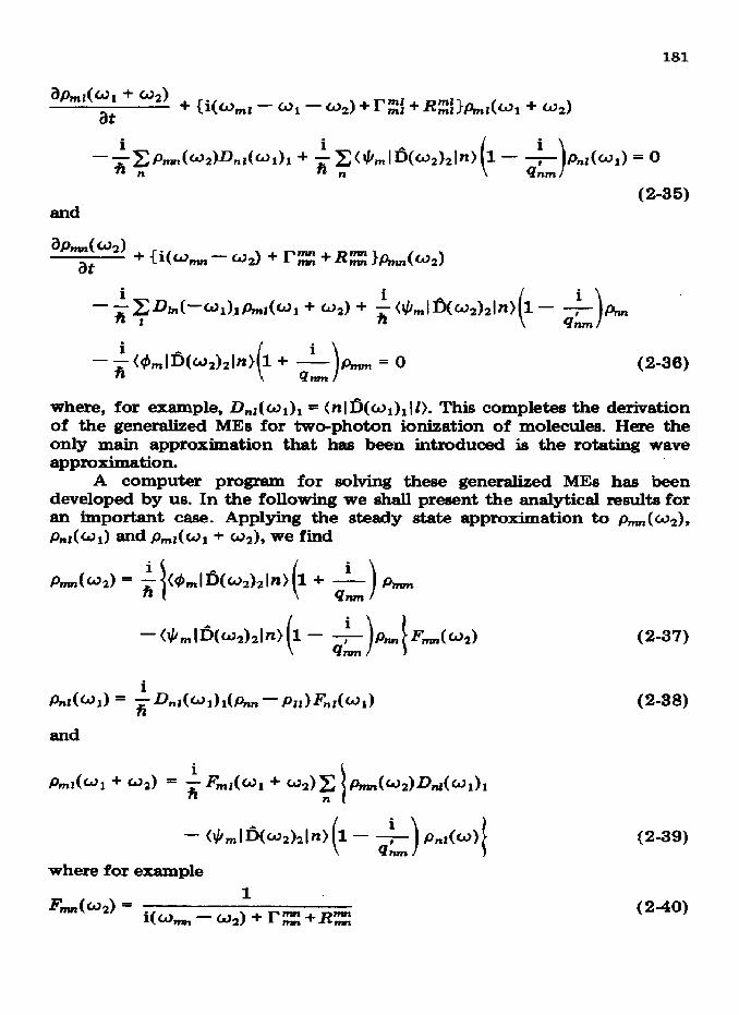
apmlwl + w2) at + Ci(wm1- Wl - 02) + rzi + Ksmr(w, + 02)

ab(W2) at

+ {i(w, - W2~+czt+~nrn~hnn(~2)

- $D”‘- .

Wl)lPm,W, + 021 + I

+ (rLmI@~2)2ln) 1 (-id,

. . -+(#mIfi(~2)2l~) I+ L &m = 0

( 1 Q?L?Pt (2-36)

where, for example, &(wl), = (n I fi( w 1)1 I I). This completes the derivation of the generalized MEs for two-photon ionization of molecules. Here the only main approximation that has been introduced is the rotating wave approximation.

A computer program for solving these generalized MEs has been developed by us. In the following we shall present the analytical results for an important case. Applying the steady state approximation to pm(02),

&z(Wd ad Prnt(Wl+ ~21, we find

PmnW2) = f ‘1

w,I~,(~2),I~> ( 1 +

-wtm~*)2l~~ I- (

i -&rim 9 nm 1

i - Pnn J7?rm(w2) dam 1 t

and .

Pml(Wl + W2) = ; enr(w1 + w2)C Pmrtw2mlzw1h n 1

- (1Lmlfi(W2)2ln) 1 - ( 2) P&)[

where for example

J??mbJn) = 1

i(w, - 02) + FE +Rz

(2-37)

(2-38)

(2-39)

(2-40)

182

‘), off-diagonal terms such as DI,(-~l)l~mI(w, + w2) obtaining eqn. (2-38) the of&diagonal terms such as

(nlfi(-&2)21q5m)~l(~I + w,) were neglected. Substituting eqns. (2-37) and (2-38) into eqn. (2-39) yields

In obtaining eqn. (2-37 were neglected and in

i ’ Pnal(Wl + w2) = h ( 1

F,l(Wl + w2)C F,,(W2)~,l(~l~l(~,I~(~Z)ZI~~ n [

i x 1+- ( > &WI - P,CF,,(Wz) + &W,~3($m lw421~>

x kq

nm

i

iis ) D,i(WII* + FnL(W1){3/rnIfi(W2)21~)

(2-41)

The validity of this approximation is examined in Appendix C. By using eqns. (2-37) - (2-41), we obtain the MEs for ~11, pnn and pm as

(2-42)

(2-43)

and

aPmm - + {R”” + A~(wz)h,m + Cknn(wz)h - c rii?‘Pmm

at n n

= $ Iab4M2 (w;J

W(r) + KW - w)~ + {r;{(r) + R”,:(r))*

(2-44)

(2-46)

&m(~d = - $ Im~i~,,(w2)31{~l~(--2)21#m}12

x Mrm CEXr) + JCW

- ~2)~ + {I’=(r) + Rz(r)}2

x (1--1/am*WiXr) + GXr)l + Wq,,)(w2 - w&J M?C aI2 + UTXr) + RRXr)32

x (1 - llqm2Hr EXr) + KW)3 - CW,,)(w2 - 4.d bdIZ?T wd2 + ~JXi#r) + Rii2W2

183

(2-46)

(2-47)

(2-46)

From eqns. (2-42) - (2-44) we obtain the differential yield of photoionization as

( h hln Y(t)=-p- +c-- ham 1 at ?I at +c--

m at 1 = 4 RZ +Ai,,&ol + c &tn(W pm

n m t

f C JGi + 4nmlo2) + C&,,(WZ) I t

pmm (2-w m n

For the weak field-weak field case [ 33, we can apply the steady state approximation to eqns. (Z-43) and (2-44) to oM,ain pm and p,_ as

‘m= Rz + W,, + Ak(w2) + PA, 1

(2-50)

and

h?z?n= ;mm+ - (2-51)

where W, = --&rr and W,, = --&J’~ represent the electronic relaxation rates of the n-level and the m-level respectively. Here the vibrational mlaxa- tion &,sI’g’&~~e and Em~l?~‘~m~m~ have been neglected. This means that either the vibrational relaxation is fast so that the vibrational equilibrium is established or the vibrational relaxation is so slow that it can be ignored. Substituting eqn. (2-51) into eqn. (2-49) ‘yields

where R, denotes the rate of direct photoionization due to the ~3~ photon originating from the n-level of the intermediate electronic excited state.

For the case W,, S RE (i.e. the case in which the electronic relaxation is much faster than the autoionixation), eqn. (2-52) reduces to

= 4 n

RE+& m 5 Ih lfic-~2~21&?a~12

x Q?mz(~a - 4m I- WExr) + ZEW3

(w2 - dnn I2 + CK3r) + ZiZW2 1 Pnn (2-53)

These results for the photoionization yield are similar to the one-photon ionization case (comparing with eqns. (2-16) case W-<Rz (i.e. the case in which the slower than the autoionization), we have

y= C(RE + &,Awa)~~nn

and (2-17)). However, for the electronic relaxation is much

n

Rz+ 2 19218(--2)21w~2

v hwn3 - UCCiXr) + JCZ(r)3 + 2q,,(w, -&?I> C4lWl - C*;)Z)’ + (r=(r) + Rz(r)j2

(2-54)

The asymmetric bandshapes in these two cases are somewhat different; the second case shows the Fano bandshape [ 41.

Other cases such as the strong field-weak field case, the weak field- strong field case, the strong field-strong field case etc. [3] can be considered similarly and will not be given here.

186

It should be noted that, although I, m and n in this section and in Figs. 1 and 2 have been referred to as representing vibronic or robronic levels of a molecule, they can of course also be referred to as higher electronic states (such as Rydberg states). In other words, by reinterpreting the models shown in Figs. 1 and 2, the theoretical results presented in this section have quite a wide range of applications. For example, they can be applied to photodissociation of van der Waals complexes or laser-stimulated desorption of adsorbed molecules.

3. Discussion

From Sections 2.1 and 2.2 for one-photon ionization and ionization of molecules, we see that the Beutler-Fano-type

two-photon asymmetric

bandshape will be observed provided U,, # 0 (autoionization matrix element) and D, # 0 (dire& photoionization matrix element). In other words, Fano’s q parameter is finite. The Beutler-Fano-type bandshape disappears if Q + 00; this can happen if either U,, = 0 orD, = 0, but D, Z 0. To see the consequence of these conditions, let us consider the one-photon ionization case. For the case U,,,, = 0, we have Ez = 0, i.e. autoionization does not take place, and eqns. (2-9) and (2-10) become

%Wl at

+ (Rz + A,)P, + xA,r4nm + c rEth,an, + 5 r$?Pn~ = 0 m m

and

aPmm +A at

mmpmm + ~&,,,P,,,, +CE,i!i’%m~m~ - CCi%n,m = 0 n m’ n

where

(3-l)

(3-2)

A am + XXr)

nm ,A_,_? ?a2 (wL-- a)2 + {r=(r) + Rz(r)}2

I(~Ifi,(--)ImN2 (3-3)

&?t =--CA_ m

(3-4)

Aam =-CA, n

As expected, the photoionization yield is dependent’only on direct photoionization, i.e.

y(t) = c Jcaln (3-5) n

Similarly, for the case D, = 0 we have RE = 0, i.e. direct photoionization does not take place. In this case, the MEs are given by

186

hln (3-6)

and

%%?W at + (Rz + A,,,&-, + CA,p, - 2 FE& + ~r~‘p,w = 0 (3-7)

n n m’

In this case, the relations given by eqns. (3-3) and (3-4) stiIl hold and the photoionization yield is dependent only on autoionization:

Y(0 = c zz&Wn (3-S) m

It should be noted that for the case q + 00 the MEs given by eqns. (3-2), (3-6) and (3-7) are the ConventionaI rate equations [ 6,6] and that the con- ventional rate equation approach usualIy cannot provide the Beutler-Fano- type bandshape for photoionization. Similar conclusions for q --f 00 can be obtained for the two-photon ionization case and will not be discussed here.

The continuum shown in Figs. 1 and 2 does not have to represent only the ionization continuum; it can represent any other type! of continuum (e.g. a dissociation continuum or separate ion-pair formation continuum etc.). In other words, the theoretical results presented in Sections 2.1 and 2.2 can also be applied to other multiphoton processes with the excited electronic state coupled to a continuum.

Several types of autoionization appear in molecular photoionization spectra 17 - 91. The kinetic energy of the ejected electron may come from the autoionization state by conversion of either the rotational energy or the vibrational energy of the ion core [7]. Another common type of autoionization involves the conversion of the electronic energy of the core and is called electrostatic autoionization [S]. One other type of autoionization, which can be called the spin-orbit autoionization, results from a transfer of the spin-orbit energy of the ion core to the photoelectron kinetic energy [ 91.

I I I 62,000 62,503 63,000

Two-color Energy/ar~-~ Fig. 3. The two-color PIE spectrum of the aniline 11 ‘Bz band.

187

Recently, Hager et ~2. [lo] have measured the two-color, threshold photoionization spectra of jet-cooled aniline, and observed vibrationally selective autoionizing Rydberg structures in these spectra, containing quanta of the non-totally symmetric vibrational modes fob, I and 15. Figure 3 shows the photoionization efficiency (PIE) spectrum for aniline photoionized from the I{ ‘Bz transition [lo]. We shall qualitatively interpret this PIE spectrum by using the theoretical results presented in this paper as follows.

Depending on whether W,, > Rz or W,, Q RE, the two-color photoionization yield can be expressed by eqn. (2-53) or eqn. (2-34). For example, for the W,, Q Rz case, we have

Y= 2 J-GE n

+ f 2 l(~l~(--w,)21&,,>12 -+ m RTtl

x %?-(wz - w-3) + (am2 - l)CCZ(r) + REXr)) (w, - dn I2 + CKXr) + REXr)12 1

Prvl

where Rg denotes the direct photoionization rate

(3-W

(3-10)

u tnlfi(-~2)2l$m)= <nIfi(--2)2l~) + f?fl (4fi(-q)2Id (3-11)

Equation (3-9) shows that the photoionizaki yield consists of two parts, one from the direct photoionization which determines the adiabatic ionization threshold, and the other from the contribution through autoionizing states I m}. Notice that the autoionization contribution to the photoionization yield is determined by the matrix element (nl6(--w,),l~,> given by eqn. (3-11). If the autoionization state Im) is a Rydberg state of high principal quantum number, then 0~I6(-~~2)~1rn) is usually much smaller than (nld(--02)alc) if c is the lowest ionic state. In this case, the direct photoionization Rg makes more contribution to Y than that through autoionization given by the second term on the right-hand side of eqn. (3-9). This is the reason why one observes a sharp adiabatic ionization threshold due to Rz_ In this case, the second term on the right-hand side of eqn. (3-11) becomes important and we see that the autoionization matrix element UC, plays an important role in determining the Rydberg structures of the PIE spectra near the threshold [lo].

To interpret the I1 i ‘B2 PIE spectrum of aniline, we use the adiabatic approximation as a basis set:

Im> = %Xl(QI)&s”’ (3-13)

188

and

Ic) = *,,&,(Q~~,,~J (3-14) where @,,, @‘b and Q1,. represent the electronic wavefunctions (see Fig. Z), X,(Qr) and XW(Q1) denote the vibrational wavefunctions of the inversion mode Qr and &,, O,# and dfV” are the vibrational wavefunctions of ail other vibrational modes. Thus for direct photoionization

where, in the second step, the Condon approximation has been introduced. Owing to the fact that the inversion mode is not totally symmetric, we can see that the most probable transition is w = 1 and u’ = u provided there is no big change in geometry between the lB2 state and the ground state of the ion. In other words, the direct photoionixation yields the step-function ionization behavior shown in Fig. 3 for the high resolution measurement.

Next we consider the autoionization contribution to the Ii ‘BP PIE spectrum. From eqn. (3-9), we can see that it is determined by the matrix elements U, m and {n Ifi(-o&Ic}. Note that for vibrational autoionization we have

(3-16)

Here again the Condon approximation has been introduced. From eqn. (3-16) we can see that the dominant transitions -are w = 0, v” = u’ and w = 2, un = vl. However, the latter transition takes place above the threshold. Thus, the Rydberg structures shown in Fig. 3 are due to the w = 0, v” = u’ transition. In this case, we have

w%--02)21d = (x,e,.i(~~iIS(--2)2t~~>Ix,e,,~.>

1 a*cJ 5(-w2)21 a,) = 391 I

(x,lQrlx,)(e,,le,,~~} 0

(3-17)

Here the vibronic coupling is introduced. vibronic coupling plays an important role 11’ lB2 PIE spectrum.

In other words, in this case the in the Rydberg structures of the

189

More recently, Kung et al. [ll] have obtained the high resolution spectra of new Rydberg states of Hz in the extreme W region by twostep doubly resonant excitation (i.e. stepwise resonant two-photon ion-pair (H+ + H-) production) followed by H- ion detection._ In other words, their experiment can be described by the following scheme: Excitutiun

hvl H2 - H2* (R ‘Cz or C ‘ll,)

M H2 + r H2**

Autoionization

Ion-pair form2 tion

H2 *‘+H++H-

For convenience of discussion, we reproduce their ion-pair production spectrum of Hz and the fitted Beutler-Fano ban&h&es in Fig. 4.

Kung et al. [ll] have fitted the observed Beutler-Fano asymmetric band&apes by using Fano’s equation (see eqn. (2-54)). As shown in Section 2, Fano’s equation can be used only when we have the weak field-weak field caseandW,,+R~. For comparison, we consider the W,, N RR case

(3-18)

V*= 9, If= 3 series

01 I I I I I ns734 753 773 m2 811 139830

TOTAL PHOTON ENERGY km”) Fig. 4. Ion-pair production qwctrum of Ha and the fitted Beutler-Fano bend&apes: -, calculated; - - . , experimental.

190

in terms of the detunings E, defined by eqn. (Z-19). As was pointed out in Section 2, the asymmetric band&ape function given by eqn. (3-18) is somewhat different from Fano’s bandshape function (see eqn. (2-20)). However, both expressions can be made to exhibit the same asymmetric bandshape by choosing the two qnrn values as follows:

cfnm(Y~ = km(F)

1 - qnm( F12 (3-19)

where g-(Y) represents the qm value given by eqn. (3-18) while q,(F) denotes the q- value for Fano’s bandshape function. For comparison these two sets of qm values for the ion-pair production spectrum of Hz are given in Table 1. Note that the widths determined from the Beutler-Fano bandshapes consist of I’;(r) and RF(r) from both m and n levels (see Appen- dix A).

Also, from eqn. (3-18) (or eqn. (2-52) for the Fano case), we can see that, within a small wavelength range, we can assume that the contribution from the direct process RE is relatively constant. In this case we can determine the ratio of the two neighboring l{n I@- w2j2 I&, >I* values (Fig. 5). Forn=25andn=26wefind

(3-20)

(3-21)

TA3LE 1

Comparison of q,,(F) and qmm( Y) v al ues of the ion-pair production spectrum of I-I2

n XZ(r) + GE(r) qnmUV= s7nmI Ylb 25 1.75 0.40 0.95 26 0.95 0.20 0.40 27 1.25 0.60 1.75 28 1.10 0.65 1.60 29 0.35 0.10 0.35 30 1.00 0.00 0.00 31 1.20 -0*30 -0.35 32 1.50 -0.30 -0.50 33 0.90 -0.80 -4.50 34 0.70 -0.80 -4.50 35 1.00 -0.15 -0.45

*From ref. 13. bOur results.

191

(3-22)

In this way we can determine the ratio

1

2

c ad-~2M-L78 whc) C i 26

1 I

2 = 0.21

C&wC--W2vLn~(~mc) I? 25

and estimate the relative magnitude of the terms (nIfi(-~~)~(rn) and

;+ 0NW---w,),lC) mc

involved in qnm.

It should be mentioned that in Fig. 5, in order to fit the experimental data, the values of qmn and R”(r) + FE(r) for n = 26 have been modified slightly from those given in Table 1 to take the values of 0.67 and 1.00 respectively. This is due to the interference between the two neighboring bands, and indicates that it is important to know the behavior of the contribution &om the direct photodissociation (or photoionization) and to take into account the interference effect in order to obtain accurate qnm and I<~I~(-w~)~I~~)~~ values. The widths FE(x) +Rz(r) are relatively insensitive to the interference effect however.

In conclusion, in this paper we have generalized our previous density formalism for the treatment of multiphoton ionization of molecules by including the effect of multirovibronic levels and have shown how to apply this theory to analyze the experimental data. It should be noted that the Green’s function formalism for multiphoton ionization of atoms has been developed by Lambropoulos and coworkers [12]. A main feature of the density matrix method is that it can properly take into account the heat bath effect represented by l?c’ in this paper. Thus the theoretical results obtained in this paper can also be applied to study photoionization of

total ohotcn energy (cm4) Fig. 5. Calculated ion-pair production spectrum of Ha for n = 25 and n = 26.

192

molecules in dense media. In this case, vibrational relaxation ls often much faster than other rate processes so that the vibrational equilibrium is established, Then, for one-photon ionization, we may set A, = p&, and pmm = p&,, where P, and Pm represent the equilibrium distributions in the ground electronic state and the excited electronic state respectively, Z,P, = 1 and Z:,P, = 1. Equations (2-9) and (2-10) yield

aPI %i- +=pg+bk=o and

aPa at

+ a’p, + b’p, = 0

where

a = c P,(R$ + A,) ?I

b = ~~PmGLrn + FE’) nm

(3-26)

(3-26)

(3-27) a'=zzA-P, nm

and

b'=CPmRz+Amm-- r m i =r 1 ”

(3-28)

In this case, all the rate constants are weighted by the equilibrium distributions P,, and Pm, and the time-dependent behaviors can be obtained by solving eqns. (3-23) and (3-24). The two-photon ionization case can be treated similarly and will not be discussed here.

Another feature of the density matrix formalism of multiphoton ionization of molecules is that the competing processes other than photoionization can be taken into account. Work is in progress to apply this formalism to study the photoionixation of liquids and solids.

Acknowledgments

This work was supported by the National Science Foundation and Arizona State University. Two of us (A-B. and S.H.L.) wish to thank Professor Hofacker of the Technical University of Munich for his gracious hospitality.

References

1 C. Y. Ng, Adv. Chem. Phys.. 62 (1983) 263. Y. Fujimura, in S. H. Lin (ea.), Advances in Multiphoton Processes and Spectroscopy, Vol. 2, World Scientific, 1986, pp. I - 75.

193

H, Kiihlewind, H. J. Neusser and E. W. SchIag, J. Phys. Chem., 89 (1986) 6600. W. Dietz, H. J. Neusaer, U. Bowl, E. W. Schlag and S. H. Lin, Chem. Phyu., 66 (1982) 105.

2 B. Fain, H. KOPO, S. H. Lin, W. E. Henke, H. L. Selzle and E. W. S&lag, & Chin. Chem. Sot.. 32 (1986) 187. Y. Fujimura and S. H. Lin,J. Chem. Phys., 75 (1981) 6110.

3 A. BoegIin, B. Fain and S. H. Lin, J. Chem. Phys., 84 (1986) 4838. 4 U. Fano, Phys. Rev., 124 (1961) 1866. 6 H. Rottke and H. Zacharias, J. Chem. Phys., 83 (1986) 4831. 6 D. S. Zakhetim and P. M. Johnson, Chem Phys., 46 (1980) 263.

V. S. Letokhov, V. I. Mishin and A. A. Puretzky, hg_ Quuntum Electron., 5 (1977) 139.

7 R, S. Ben-y. J. Chem. Phye.. 45 (1966) 1228. U. Fano, Phys. Reu. A, 2 (1970) 363.

8 M. Raoult, H. Le ROUZO, G. Raaeev and H. Lefebre-Brian, J. Phye. B, 16 (1983) 4601. 9 H. Lefebre-Brion, A. Giusti-Suzon and G. Raseev, J. Chem. Phys., 83 (1985) 1657.

10 J. Hager, M. A. Smith and S. C. Wallace, J. Chem. Phys., 83 (1986) 4820;84 (1986) 6771.

11 A. H. Kung, R. H. Pege, R. J. Larkin, Y. R. Shen and Y, T. Lee, Phys. Rev. Let+, 56 (1986) 328.

12 P. Lambropoulos and P. Zoller, Phys. Rev. A, 24 (1981) 379. Y. S. Kim and P. Lambropouloa, Phys. Rev. A, 29 (1984) 3169.

Appendix A: Derivation of eqns, (2-l) - (2-20)

Consider pm given by eqn. (2-7). Notice that

= 2Re (A-1)

Here eqn. (2-3) has been used. Writing k(t) as

pm(#) = h(w) exp(-itw) + p-(--o) exp(iU) (A-2) and using eqn. (2-4) and the rotating wave approximation, we obtain

(A-3)

where

(A-4)

Equation (A-3) can be written as

Substituting eqn. (A-5) into eqn. (2-7) yields

(A-7)

SimiIarIy, eqn. (2-6) becomes

kk +R~p_+Crmmpkk=O (A-8)

k

where

(A-9)

and

1 Wf0~~“.c--O)U,,WJ -WC,)

c -= I Qlw?a (~Ifi(--)Iha)

(A-10)

It is commonly assumed that qnnr = q;, and WI@--w)IJI,) = (nIfi(-WI@,) and that Q- is a real number. This assumption wiII be examined in a future investigation.

Using the relations

exp(ito) (’ ;I.&+R& (A-11)

and *

exp(ifw) =+&w)ln)

we can rewrite eqn. (2-8) as

%nza(~) at

+ {i(o- - W) + RE + rZ)~mn(~)

195

(A-12)

p_=O

(A-13)

Applying the steady state approximation to h(w) yields

&ivaw) = (i/~)(~,I~(w)In}(l+ilq,)p,, -(il~){~/,I~,(.~)In)(l-ii/q~,)hur

‘i(w, -a) + R& + rg (A-14)

Equations (2-9) and (2-10) are obtained by substituting eqn. (A-14) into eqns. (A-7) and (A-8). Notice that

i<n~~~--W)l~,>(rLmI~(~)l~)ll- i/q,Al-~i/dm) i(w, - o)+RE+rE I.

(A-15)

2 A

ilG$,I~,(~)l~~12~l + 1/qnm2) nm=--

A2

Im i(0, - a)+Rz+rE I

(A-16)

A_=-$ Im i IW,I fi,l@ ld12(1. + 1/qk2)

i(w, - w)+RZ+ryg (A-17)

and

i<nl~(-_)I~m)(9mI~(~)t~)(l+ i/aLN+ i/a,) i(w, - cd)+Rz+rz

(A-18)

Here the only assumption inWxh_~ced is that qnm and qh are real. Further assumptions of I$, = J/, and qnm = qk will reduce the above expressions for A A,, M, A, and A- to those given in Section 2.

Next we consider the calculation of Rz. Using eqn. (2-3) we find

R~=J,,+J~ = Rg(r) + iRE(i) (A-19)

and from eqn. (2-4) we obtain

(A-20)

and

J, = (A-21)

Substituting eqns. (A-20) and (A-21) into eqn. (A-19) yields

R=(r) = $(RE + RZ)

and

(A-22)

R=(i)= (A-23)

Xn other words, R=(r) and R=(i) represent the level width and level shift due to autoionization and direct photoionization. Similarly, it has been shown that the dephasing constant l?” due to the coupling between the system and the heat bath can also be written as [Al, A2]

FE = r=(r) + W=(i) (A-24)

Thatis,itcanalsobewrittenasthe summation of the level width and the level shift. It should be noted that

r%(r) = +(rz+rz)+rE(d) (A-26)

where r=(d) d enotes the pure dephasing. Equation (A-25) indicates that l?=(r) has contributions not only from the lifetimes of the m-level and the n-level but also from the pure dephasing.

Next we consider an important case, qm = 0. We find 1

(~Ifi(-~)I$m)- = $pnc( --O)~mn~(~na~)= Gm (A)

Qrv?t c

~nlfN--w)lJ/m)+ = &&(--W)UemS(W -we,) = &t UV

A ,A_P-~ rm2CCZ(r) + Rm”(r)l nm ti2 (cd:,- cd)2 + {R=(r) + rE(r)12

An = ~&,,a m

and

Aam= ~&an n

(Cl

(D)

w Here for convenience we have assumed that r;, = rk. The above results show that for this particular transition n * m the bandshape is lorentzian:

Y = C(R,M + 2&&q,,, + C (Rm” + 24,.&m w n m

197

References for Appendix A Al S. H. Lin and H. Eyring,&x. N&L. Acud. Sci U.S.A., 74 (1977) 3623. A2 B. Fain and S. H. Lin, Surf. Sci., 147 (1984) 497.

B. Fain, A. R. Ziv, G. S. Wu and S. H. Lin, in S. H. Lin (ed.), Advances in Multi- photon Procemes and Spectromopy, Vol. 1, World Scientific, 1984, pp. 420 - 500.

Appendix B: Derivation of eqns. (2-21) - (2-64)

First we consider &l(t) given by eqn. (2-31). Notice that &l(t) = AI(W) exp(--itW + hr(-0) exp(itwl) P-(t) = I-)mn(w~) exp(--itw?) + ~J--o~) exp(itw2) and

(B-U (B-2)

Pm2(t) = pm&W + 02) expC-iHwI + 02): + PA-w1 - w2) expW(wI + wz)} (B-3)

Substituting eqm. (B-l) and (B-3) into eqn. (2-31) and using the rotating wave approximation, we find

aP"l(wl) .

at + {i(w,r - WI) + rR,; + R::f~n,lW + f Qll(wlMm - Pm)

V,, + Rz/ exp(- itw&,Awl + ~21 = 0 (B-4)

Notice that .

exp(-itwl) = $ &d--2)2Jnm expWtw2) (B-m

and

Jnm exp(-itw2) =

where

fi = @wl)l exp(-itw,) + G(-wl)l exp(itwJ + d(w,), exp(-itw2) + 5(- w~)z exp(itw 2)

Substituting eqn. (B-6) into eqn. (B-5) yields

(B-7)

( .

f V,, + RF: exp(-itw,) = * )

i (nIfi(-W2)2l@,) 1 EL)

and eqn. (2-34) is obtained by introducing eqn. (B-8) into eqn. (B-4).

198

consider hl( t) given by eqn. (2-32). Again substituting eqns.

we obtain into eqn. (2-32) and using the rotating wave approximation,

Next we (B-l) - (B-3)

aPrnZ(w + 02)

at +Ci(o,Z - "1--w?) +xi +~~;bZ(~l+ 01) . .

+c i hAw212 + Jm expWw2) h(W - + P~(c~~VMC~A I I

= 0 n

(B-9)

where we have

J- =PWw2) = .fi2 L C umcDcn(~2)2 c

+ 7mw2 - an) I

(B-10) CrS

It foUows that .

~D-(w~)~ + J,, exp(itw,) = .

where

Ika>= Im>+ g-F, u’“, Ic) 2 en

(B-11)

(B-12)

and

1 la/fi)C UmcDcnIW2)26(W2 - wcn)

C -I , Qnm <&nIJ3’(w2)2h~

(B-13)

Equation (2-35) for pmr( w1 + 02) is obtained by substituting eqn. (B-11) into eqn. (B-9).

Finally we consider p-(t) given by eqn. (2-33). Substituting eqns. (B-2) and (B-3) into eqn. (2-33) yields

%3?a(w2)

at + {i(o,- w2)+~~+JczIP,(~z)- wlPmzwl+~2)

.

+P?l” ~&dw2)2+=p(itw2)J,,

. -~D-(w~)~+ exp(itw,) Jzm

= 0

where (B-14)

(B-15)

and

exp(itw*)J& =

. .

f awlW2)2 + exp(itw&J_ = ti l WllI%~2)2l~) 1 (-k)

and

199

(B-16)

(B-17)

(B-18)

Substituting eqns. (B-17) and (B-18) we obtain eqn. (Z-36).

Appendix C: Validity of eqn. (2-41)

The performance of the steady state approximation applied to &I( wl), p,,,l(wl + 02) and p-(0,) has been examined in a previous paper [Cl]. Here we shall study the additional approximation associated with the multilevel system. Using eqn. (2-41), we obtain the improved expressions for p,JtiJ and ~mnW2) as

.

AIEW) = + &A&+) (C-1)

and

--(3/mIfii(w2)2I~> 1- ( &+rm[ +&~mWa) (C-2)

where Apnr( w 1) and Ap,( wi) represent the correction terms for A~( w 1) and pmn (~2) respectively, and they are given by

AP,,(wI) = - ; KlZ(~l)~ ~~Ifi,(--w,M9hn) P??AWI + w2) m

Frnzto, + w2)

x c ~-~(ws)~,rr(w1)1(~,I~‘(W2)*(n’) 1+ ?l’ 1

( -J--)P_ -P&n)

200

x CFmn~(~2) + Fnrr(Wl)3(~mI~(L32)21n’) 1 ( - &) D?d%h

+ Fnrl(wl)(~ml~(~*)*ln’} 1 (-3 1 Dn~l(wlPl* W-3)

+ F,~,(o,){~,I~~~2)2In’) (C-4)

These correction terms are indeed higher order terms.

Reference for' Appendix C Cl A. Boeglin, B. Fain and S. H. Lin, J Chem. Phys., 84 (1986) 4838.

Documents

A theoretical study of two-color photoionization and autoionization of molecules