A Theoretical Limit of Radar Parameter Estimation

JOURNAL OF LATEX CLASS FILES, VOL. XX, NO. X, FEBRUARY 2021 1

Theoretical Limit of Radar Parameter Estimation

Dazhuan Xu∗, Han Zhang∗, Weilin Tu∗

∗College of Electronic and Information Engineering,

Nanjing University of Aeronautics and Astronautics, Nanjing, China

Abstract

In the field of radar parameter estimation, Cramer-Rao bound (CRB) is a commonly used theoretical limit.

However, CRB is only achievable under high signal-to-noise (SNR) and does not adequately characterize per-

formance in low and medium SNRs. In this paper, we employ the thoughts and methodologies of Shannon’s

information theory to study the theoretical limit of radar parameter estimation. Based on the posteriori probability

density function of targets’ parameters, joint range-scattering information and entropy error (EE) are defined to

evaluate the performance. The closed-form approximation of EE is derived, which indicates that EE degenerates to

the CRB in the high SNR region. For radar ranging, it is proved that the range information and the entropy error

can be achieved by the sampling a posterior probability estimator, whose performance is entirely determined by the

theoretical posteriori probability density function of the radar parameter estimation system. The range information

and the entropy error are simulated with sampling a posterior probability estimator, where they are shown to

outperform the CRB as they can be achieved under all SNR conditions.

Index Terms

Theoretical limit; Parameter estimation; Range information; Entropy error; Sampling a posterior probability

estimation;

I. Introduction

Dazhuan Xu is the Corresponding Author

arX

iv:2

107.

0498

6v1

[cs

.IT

] 1

1 Ju

l 202

1

2 JOURNAL OF LATEX CLASS FILES, VOL. XX, NO. X, FEBRUARY 2021

STARTING from the pioneering work of Shannon [1], information theory has been widely applied

in communication for more than half a century. Shannon’s information theory provides theoretical

limits for communication systems. Specifically, channel capacity is the limit for channel coding and rate

distortion function is the limit for lossy source coding. The application of information theory in the radar

signal processing traces back to the 1950s. Woodward and Davies [2] adopted the inverse probability

principle to study the mutual information and obtained the approximate relationship among the range

mutual information [3], the time-bandwidth product and the SNR of a single target with constant coefficient

[4]. In [5], [6], Bell presents adaptive waveform design algorithms based on a mutual information measure,

and show more series of information of the targets can be extracted from the received signals.

The main goal of radar systems is to detect, localize, and track targets based on the reflected echoes

[7]–[9]. The echoes can be exploited to extract useful information of the target [10]–[12], including

range, velocity, shape, and angular [13], [14]. To characterize the accuracy performance of the parameter

estimator, lower bounds on the minimum mean square error (MSE) in estimating a set of parameters from

noisy observations are widely used for problems where the exact minimum MSE is difficult to evaluate.

Such bounds provide the unbeatable performance limits of any estimator in terms of the MSE. They can

be used to investigate fundamental limits of a parameter estimation problem, or as a baseline for assessing

the performance of a specific estimator. The most commonly used bounds include the Cramer-Rao bound

(CRB) [15]–[17], the Barankin bound [18], the Ziv–Zakai bound [19]–[21], and the Weiss–Weinstein

bound [22], [23]. The related works are presented as follows.

A. Related Work

It is known that the variance of unbiased estimates provided by any method is always lower bounded by

the CRB [24], [25], which provides the ultimate limitation on the resolvability of the signals, independent

of the estimation method used. Furthermore, the CRB is achieved by maximum likelihood (ML) estimators

in the limit of small noise under standard regularity conditions [26], [27]. However, the CRB does not

adequately characterize the performance of unbiased estimators outside of the asymptotic region. The

SHELL et al.: BARE DEMO OF IEEETRAN.CLS FOR IEEE JOURNALS 3

Barankin bound is tighter than the CRB. However, it is more difficult to evaluate and requires optimization

over a set of test points.

The Ziv–Zakai and Weiss–Weinstein bounds are Bayesian bounds which assume that the parameter is

a random variable with known a priori distribution. They provide bounds on the global MSE averaged

over the a priori probability density function (PDF). These bounds are tight and reliable in all regions of

operation. However, as they bound the global MSE, they can be strongly influenced by the performance at

the parameter values which have the largest errors. Also, the ZZB requires evaluation of several integrals,

while evaluation of the Weiss–Weinstein bound involves choosing test points and inverting a matrix.

The theoretical limits in this paper have been presented in our previous works. The concept of the

spatial information was proposed in 2017 [28], which unifies the range information (RI) and the scattering

information in a unified framework. In 2019, the concept of entropy error (EE) was put forward [29] as

a metric for parameter estimation systems. However, the empirical RI and empirical EE of different

parameter estimators were not addressed, and the achievability of RI and EE was not explored.

B. Motivation and Contributions

The limits mentioned above are proposed by providing bounds on the MSE, but the MSE is inherently

flawed. The reason is that MSE, as a second-order statistic, has good evaluation performance when the

statistical property for the estimated parameter obeys a Gaussian distribution, but in low and medium SNR,

the error statistics are generally not second-order values and MSE no longer reflects the performance of

the estimator accurately.

In this paper, we study theoretical limits of parameter estimation in terms of the posterior PDF and the

posterior entropy. Since entropy can reflect the degree of uncertainty in the parameter estimation system,

entropy-based metrics are proposed to evaluate the performance of radar parameter estimation. The main

contributions of this paper are summarized as follows

1) Joint range-scattering information is proposed as the positive metric, which is defined as the difference

between a priori entropy and a posteriori entropy. Range-scattering information is equivalent to the sum


of RI and the scattering information conditioned on the known range. It is proved that acquiring 1 bit of

RI is equivalent to doubling the estimation accuracy.

2) EE is presented as the negative metric, which is defined as the entropy power of the differential

entropy of the posteriori PDF. The closed-form approximation of EE indicates that EE is a generalization

of MSE and degenerates to MSE in high SNR regime. Compared to MSE, RI and EE provide better

measures of estimators’ performance in low and medium SNRs. The reason is that RI and EE are based

on the posterior entropy and can reflect uncertainty in estimation results under all SNR conditions.

3) Parameter estimation theorem is put forward, which states that the RI and the EE are achievable under

all SNR conditions. To prove the theorem, a stochastic parameter estimator named sampling a posterior

probability (SAP) is proposed, whose performance is entirely determined by the theoretical posteriori PDF

of the radar parameter estimation system. As common radar systems tend to work under low and medium

SNR conditions, RI and EE are of practical significance for the reason that they can be achieved under

all SNR conditions.

C. Organization and Notations

The rest of the manuscript is organized as follows. Section II establishes a radar system model, which is

equivalent to a communication system with joint amplitude, phase, and time delay modulation. In Section

III, range-scattering information and EE are proposed to evaluate the performance of estimation methods.

Section IV introduces ML and MAP estimation methods and proposes the SAP estimation method. In

Section V, the parameter estimation theorem is proposed. Simulation results are presented in Section VI.

Finally, Section VII concludes our work.

Notations: Throughout the paper, a denotes a scalar, a denotes a column vector and A denotes a set.

The superscripts {·}∗ denotes the conjugate, {·}′ is the derivative of a function. E(·) is the expectation, Re{·}

stands for the real part of a complex number, the operators (·)T and (·)H denote transpose and conjugate

transpose of a vector respectively. A Gaussian variable with expectation a and variance σ2 is denoted by

N(a, σ2).


II. RADAR SYSTEM MODEL

In a radar system, the receiver collects some echoes when the transmitted signal is reflected by some

unknown targets. We focus on the radar parameter estimation in this paper such that there are two

characteristics that we are interested in, namely, the ranges between the targets and the receiver, and

the scattering properties of different targets. To simplify the model, we have to make some assumptions

regarding targets, range X and scattering properties S.

A1 Targets are points in observe interval.

A2 Different targets are independent. For instance, the joint PDF of target 1 and target 2 satisfies

p(x1, x2, s1, s2) = p(x1, s1)p(x2, s2).

A3 In the observation interval, the signal attenuation with distance can be ignored and the SNR can be

considered as an invariant.

Without loss of generality, let sl = αle jφl denote the complex reflection coefficient of the l-th target

and dl denote the distance between the l-th target and the receiver, for l = 1, ...,L. Down converting the

received signal to base band, the radar system equation is shown as follows

y(t) =

L∑l=1

slψ (t − τl) + w(t) (1)

where ψ(·) denotes the real base band signal and carrier frequency is fc, then the phase of the transmitted

signal can be expressed as ϕl = −2π fcτl + ϕl0 where φl0 denotes the initial phase, τl = 2dl/v denotes the

time delay of the l-th target and v is the signal propagation velocity of the signal. w(t) is the complex

additive white Gaussian noise (CAWGN) with mean zero and variance N0/2 in its real and imaginary parts,

respectively. The above equation describes a radar system model, which is equivalent to a communication

system with joint amplitude, phase, and time delay modulation.

For the convenience of theoretical analysis, it is assumed that the reference point is located at the

center of the observation interval and the observation range is [−D/2,D/2), which is shown in Fig. 1(a).


2D

2D d

(a)

2T

2T

2d

v

(b)

2N

2N x B

(c)

Fig. 1: (a) Observation distance interval (b) Observation time interval (c) Normalized observation interval.

The time delay interval is [−T/2,T/2), which is shown in Fig. 1(b). It is also assumed that the emitted

base-band signal is an ideal low-pass signal with base band B/2, that is

ψ(t) = sinc(Bt) =sin(πBt)πBt

(2)

Suppose T � 1/B, or BT � 1, the observation interval is much wider than the main lobe width of the

signal, the signal energy is nearly entirely within the observation interval

Es =

∫ T/2

−T/2ψ2(t)dt = 1 (3)

The corresponding spectrum is given by

ψ( f ) =

1B , | f | ≤

B2

0, others(4)


According to the Shannon-Nyquist sampling theorem, y(t) can be sampled with a rate B to obtain a

discrete form of (1), which is shown in Fig. 1(c)

y{ n

B

}=

L∑l=1

slψ{n − Bτl

B

}+ w

{ nB

}, n = −

N2, . . . ,

N2− 1 (5)

where N is the time bandwidth product (TBP) and satisfies N = T B. Let xl = Bτl represent the range, the

discrete form system equation can be expressed as

y {n} =

L∑l=1

slψ {n − xl} + w {n} , n = −N2, . . . ,

N2− 1 (6)

where the auto-correlation function [2] of Gaussian noise is

R(τ) =N0B sin πBτ

2πBτ(7)

It can be obtained from eq. (7) that the discrete noise sample values w(n) obtained at the sampling rate B

are irrelevant. Furthermore, since the w(n) are complex Gaussian random variables, they are independent

of each other. For convenience, write eq. (1) in vector form

y = U (x) s + w (8)

where y = [y(−N/2), . . . , y(N/2 − 1)]T denotes received signal, s = [s1, . . . , sL]T denotes target scattering

vector and U (x) = [u(x1), . . . , u(xL)]T denotes matrix determined by the transmitted signal waveform and

the range. Its l-th column vector u(xl) = [sinc(−N/2 − xl), . . . , sinc(N/2 − 1 − xl)]T is the echo from the

l-th target, w = [w(−N/2), . . . ,w(N/2 − 1)]T is the noise vector whose components are independent and

identically distributed complex Gaussian random variables with mean value 0 and variance N0.

A. Statistical Model of Target and Channel

The statistical properties of target in the radar parameter estimation system is the joint PDF of range

and scattering, which corresponds to the source and the channel in the communication system

p (x, s) = π (x) π (s) (9)


where π(x) is the priori PDF of the range, π(s) is the PDF of the scattered signal. In this paper, target

range and scattering are uncorrelated.

Without priori information, the range is assumed to obey uniformly distribution in the observation

interval. Statistical models of scattering signals have been established for different scattering scenarios. In

this paper, only two typical statistical models of radar electromagnetic scattering signals, constant modulus

(Swerling 0) and complex Gaussian (Swerling 1) are considered. The statistical properties of two kinds

of scattered signals can be expressed as

π(s) = π(α)π(ϕ) =

1

2πδ (α − α0) Swerling 0,

12π

ασ2α

exp(− α2

2σ2α

)Swerling 1.

(10)

III. PERFORMANCE EVALUATION OF RADAR PARAMETER ESTIMATION

A. Posterior PDF of Range and Scattering

The foundation of our theoretical limits is the posterior PDF. In single-target scenario, assume the

amplitude is constant and noise w is complex additive white Gaussian. The multi-dimensional PDF of

the received signal y is

p(y | x,ϕ) =

(1πN0

)N

exp

− 1N0

N/2−1∑n=−N/2

|y(n) − αejϕ sinc(n − x)|2 (11)

As p(y | x) =∫ 2π

0p(y | x,ϕ)p(ϕ)dϕ

p(y | x) =

(1πN0

)N

exp

− 1N0

N/2−1∑n=−N/2

y(n)2 + α2

1

2π

∫ 2π

0exp

2αN0

Re

e−jϕN/2−1∑

n=−N/2

|y(n)sinc(n − x)|2 dϕ

(12)

Introduce the first kind zero-order modified Bessel function

p(y | x) =

(1πN0

)N

exp

− 1N0

N/2−1∑n=−N/2

y(n)2 + α2

I0

2αN0

N/2−1∑n=−N/2

|y(n)sinc(n − x)|2 (13)

Discard the unrelated terms with x in the above equation and write it in vector form

p(y | x) ∝ I0

[2αN0

∥∥∥UHy∥∥∥2

2

](14)


where UH = [sinc(−N/2 − x), · · · , sinc(N/2 − 1 − x)] and y = [y(−N/2 − x), · · · , y(N/2 − 1 − x)]. The

inside of the 2-norm is the output of y through the matched filter. According to the Bayes’ formula, the

posteriori PDF of range is

p(x | y) =p(y | x)π(x)∫ N/2

−N/2p(y | x)π(x)dx

∝ π(x)I0

[2αN0

∥∥∥UHy∥∥∥2

2

](15)

For a snapshot, targets are assumed to be at x0 and the scattering signal is αejϕ0 . Substituting eq. (6)

to eq. (15)

p(x | w) =

I0

{2αN0

∣∣∣∣∣∣ N/2−1∑n=−N/2

[αejϕ0sinc (n − x0) sinc(n − x) + w0(n)sinc(n − x)

]∣∣∣∣∣∣}

Z(α, n)(16)

where Z(α, n) equals to the integral of the numerator on the range x. Extract the αejϕ0 in the summation

symbol

p(x | w) =

I0

{2α2

N0

∣∣∣∣∣∣ N/2−1∑n=−N/2

[sinc (n − x0) sinc(n − x) + 1

αe−jϕ0w0(n)sinc(n − x)

]∣∣∣∣∣∣}

Z(α, n)(17)

When the N is large enough, according to the properties of sinc signal

N/2−1∑n=−N/2

sinc (n − x0) sinc(n − x) = sinc (x − x0) (18)

as e−jϕ0 in eq. (17) does not affect the value in the absolute value sign

p(x | w) =I0

{ρ2

∣∣∣sinc (x − x0) + 1αw(x)

∣∣∣}∫ N/2−1

−N/2I0

{ρ2 | sinc (x − x0) + 1

αw(x)

∣∣∣} dx(19)

where ρ2 = 2α2/N0 and w(x) satisfies

w(x) = e−jϕ0

N/2−1∑n=−N/2

w0(n) sinc(n − x) (20)

w(x) is still a Gaussian white noise process with zero mean and N0 variance. From the expression

of p(x | w), it can be seen that the posterior PDF is symmetric centered on the target location. The

shape of the posterior PDF is completely determined by the numerator, and the denominator only plays

a normalizing role. Let 1αw(x) =

√2ρµ(x), another posterior PDF expression can be obtained

p(x | µ) =

I0

[ρ2

∣∣∣∣sinc (x − x0) +√

2ρµ(x)

∣∣∣∣]∫ T B/2

−T B/2I0

[ρ2

∣∣∣∣sinc (x − x0) +√

2ρµ(x)

∣∣∣∣] dx(21)


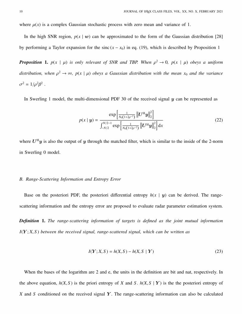
where µ(x) is a complex Gaussian stochastic process with zero mean and variance of 1.

In the high SNR region, p(x | w) can be approximated to the form of the Gaussian distribution [28]

by performing a Taylor expansion for the sinc (x − x0) in eq. (19), which is described by Proposition 1

Proposition 1. p(x | µ) is only relevant of SNR and TBP. When ρ2 → 0, p(x | µ) obeys a uniform

distribution, when ρ2 → ∞, p(x | µ) obeys a Gaussian distribution with the mean x0 and the variance

σ2 = 1/ρ2β2 .

In Swerling 1 model, the multi-dimensional PDF 30 of the received signal y can be represented as

p(x | y) =

exp[

1N0(1+2ρ−2)

∥∥∥UHy∥∥∥2

2

]∫ N/2−1

−N/2exp

[1

N0(1+2ρ−2)∥∥∥UHy

∥∥∥2

2

]dx

(22)

where UHy is also the output of y through the matched filter, which is similar to the inside of the 2-norm

in Swerling 0 model.

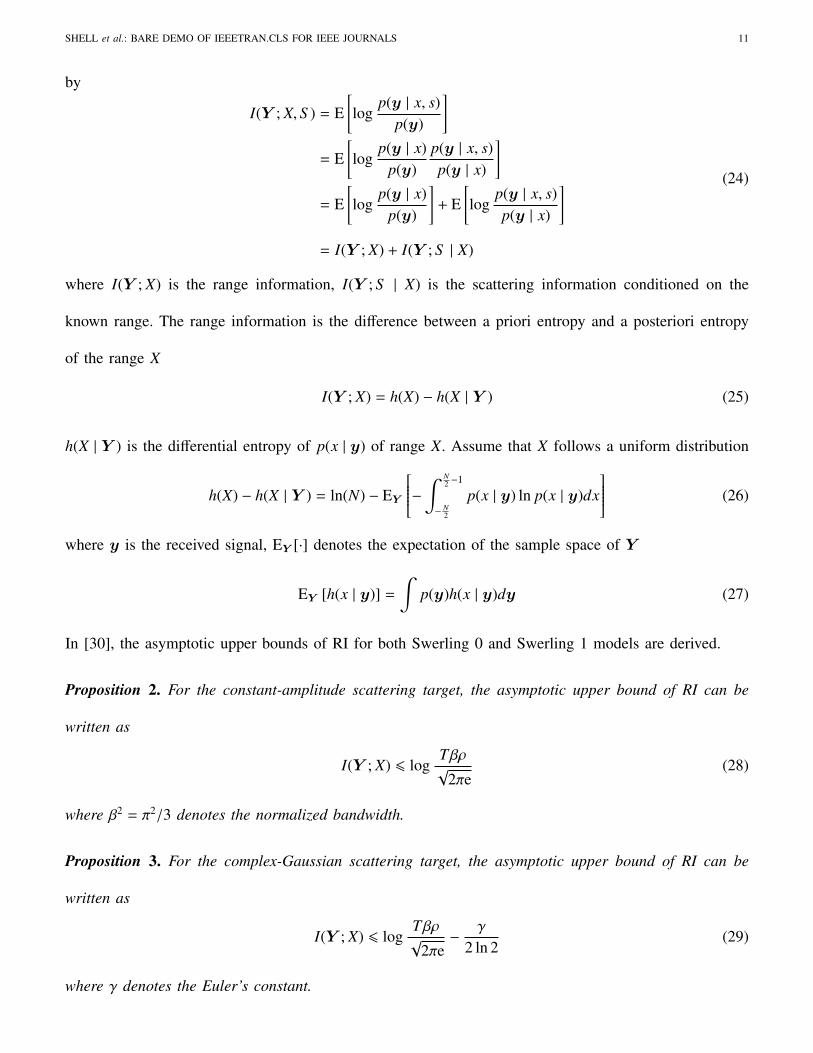
B. Range-Scattering Information and Entropy Error

Base on the posteriori PDF, the posteriori differential entropy h(x | y) can be derived. The range-

scattering information and the entropy error are proposed to evaluate radar parameter estimation system.

Definition 1. The range-scattering information of targets is defined as the joint mutual information

I(Y ; X, S ) between the received signal, range-scattered signal, which can be written as

I(Y ; X, S ) = h(X, S ) − h(X, S | Y ) (23)

When the bases of the logarithm are 2 and e, the units in the definition are bit and nat, respectively. In

the above equation, h(X, S ) is the priori entropy of X and S . h(X, S | Y ) is the the posteriori entropy of

X and S conditioned on the received signal Y . The range-scattering information can also be calculated


by

I(Y ; X, S ) = E[log

p(y | x, s)p(y)

]= E

[log

p(y | x)p(y)

p(y | x, s)p(y | x)

]= E

[log

p(y | x)p(y)

]+ E

[log

p(y | x, s)p(y | x)

]= I(Y ; X) + I(Y ; S | X)

(24)

where I(Y ; X) is the range information, I(Y ; S | X) is the scattering information conditioned on the

known range. The range information is the difference between a priori entropy and a posteriori entropy

of the range X

I(Y ; X) = h(X) − h(X | Y ) (25)

h(X | Y ) is the differential entropy of p(x | y) of range X. Assume that X follows a uniform distribution

h(X) − h(X | Y ) = ln(N) − EY

−∫ N2 −1

− N2

p(x | y) ln p(x | y)dx

(26)

where y is the received signal, EY [·] denotes the expectation of the sample space of Y

EY [h(x | y)] =

∫p(y)h(x | y)dy (27)

In [30], the asymptotic upper bounds of RI for both Swerling 0 and Swerling 1 models are derived.

Proposition 2. For the constant-amplitude scattering target, the asymptotic upper bound of RI can be

written as

I(Y ; X) 6 logTβρ√

2πe(28)

where β2 = π2/3 denotes the normalized bandwidth.

Proposition 3. For the complex-Gaussian scattering target, the asymptotic upper bound of RI can be

written as

I(Y ; X) 6 logTβρ√

2πe−

γ

2 ln 2(29)

where γ denotes the Euler’s constant.


For the complex-Gaussian amplitude scattering target, the scattering information I(Y ; S | X) is given

by the following equation

I(Y ; S | X) = h(Y | X) − h(Y | X, S ) (30)

As is derived in [30], the scattering information satisfies

I(Y ; S | X) = log(1 +

ρ2

2

)(31)

The above equation is consistent with the Shannon’s channel capacity formula. As can be seen from the

above equation, I(Y ; S | X) is independent of the normalized time delay of the target, i.e., the scattering

information is independent of the RI.

Definition 2. The entropy error is defined as the entropy power of the posteriori PDF p(x, s | y), which

can be expressed as

σ2EE (X, S | Y ) =

22h(X,S |Y )

2πe(32)

and the square root of the entropy error is named as the entropy deviation σEE (X, S | Y ).

The entropy error of range-scattering can also be calculated by

σ2EE (X, S | Y ) = σ2

EE (X | Y ) · σ2EE (S | X,Y ) (33)

where σ2EE (X | Y ) is the entropy error of range, σ2

EE (S | X,Y ) is the entropy error of scattering conditioned

on the known range. For the constant-amplitude scattering target, the range is of more concern. The

definition of entropy error of range is shown as follows

σ2EE (X | Y ) =

22h(X|Y )

2πe(34)

As is derived in [31], the approximation for posteriori entropy of single target is written as

h(X | Y ) = psHs + (1 − ps) Hw + H (ps) (35)

where Hs is the normalized a posteriori entropy in high SNR region, which can be represented as

Hs =12

ln(2πeσ2

)= ln

B√

2πeρβ

(36)


Hw is the normalized a posteriori entropy in low SNR region, which satisfies

Hw = lnNρ√

2π

eρ2+1

2

(37)

H (ps) denotes the uncertainty of the target, which can be expressed as

H (ps) = −ps log ps − (1 − ps) log (1 − ps) (38)

where ps is called ambiguity, which denotes the probability that the target range is around x0 and can be

written as

ps =exp

(ρ2/2 + 1

)Tρ2β + exp

(ρ2/2 + 1

) (39)

The approximation for EE of single target is shown in Proposition 2 and the proof is in the Appendix.

Without causing confusion, σ2EE refers to the entropy error of range σ2

EE (X | Y )

Proposition 4. The approximation for EE of single target is

σ2EE =

1ρ2β2 p2

s(40)

Thus, EE is a generalization of the MSE and degenerates to the CRB in the high SNR region.

Entropy deviation is closely related to RI. Let σEE(x) denotes the entropy deviation of the priori PDF

p(x) and σEE(x|y) denote the entropy deviation of the posteriori PDF p(x | y)

σEE(X | Y )σEE(X)

= 2h(X|Y )−h(X)

= 2−I(Y ;X)

(41)

where I(Y ; X) represents RI. The relationship of RI and entropy deviation is stated in the Theorem 1

Theorem 1. Acquiring 1 bit range information is equivalent to reducing the entropy deviation by half.

The RI represents the amount of information acquired and the EE represents the accuracy of the

parameter estimation, which are equivalent. Thus, both RI and EE can evaluate the performance of

estimators.


IV. Sampling a Posterior Probability Estimation

ML estimation and maximum a posteriori probability (MAP) estimation are two typical deterministic

estimation methods, whose estimation values for the same received signal are the same.

In Swerling 0 model, the estimation value that maximizes p(x | y) in eq. (15) is called maximum a

posterior probability estimation of the range x, which is denoted as xMAP

xMAP = arg maxx

π(x)I0

2αN0

∣∣∣∣∣∣∣N/2−1∑

n=−N/2

y(n) sin c(n − x)

∣∣∣∣∣∣∣ (42)

The estimation value x that maximizes p(y | x) in eq. (14) is called the maximum likelihood estimation

of the range x, which is denoted as xML

xML = arg maxx{p(y | x)}

= arg maxx

I0

2αN0

∣∣∣∣∣∣∣N/2−1∑

n=−N/2

y(n) sinc(n − x)

∣∣∣∣∣∣∣ (43)

If the range X follows uniform distribution in the observation interval N, its prior PDF satisfies π(x) =

1N , the π(x) in eq. (15) can be omitted. The denominator is a normalization of the numerator and does

not change the shape of the posteriori PDF, xMAP can be represent as

xMAP = arg maxx

I0

2αN0

∣∣∣∣∣∣∣N/2−1∑

n=−N/2

y(n) sin c(n − x)

∣∣∣∣∣∣∣ (44)

It can be seen from the above equation that ML is equivalent to MAP under the premise that range X

obeys a uniform distribution.

Corresponding to random-coding method in communication, we propose SAP estimation method, which

can be expressed as

xSAP = arg smpx{p(x | y)} = arg smp

x{p(y | x)π(x)} (45)

where arg smpx{·} denotes the sampling operation. If x satisfies the uniform distribution, π(x) in the above

equation can be omitted.

For the sake of simplicity, only the single target case is considered. The sampling operation can be

represented as follows


Fig. 2: Block diagram of a simplified radar ranging system.

1) The whole observation interval is divided into several small intervals [x0, x1), [x1, x2), · · · , [xK−1, xK],

the probability of k-th interval is obtained by calculating the integral of the posterior PDF, which can

be expressed as pk(x | y) =∫ xk

xk−1p(x | y)dx.

2) p1(x | y), p2(x | y), · · · , pK(x | y) are used to sample. Larger values is, more likely the corresponding

interval is sampled.

3) Output the center points of the sampled intervals as the xSAP.

As the snapshot number M increases, the statistical distribution of xSAP will approach the theoretical

PDF of x, while the statistical distribution of the output of deterministic estimation methods is difficult

to determine.

The differential entropy of SAP is invariant, which means that the actual range x0 only affects the

position but not the shape of the posteriori PDF p(x|y(x)), and differential entropy is not related to x0.

The posteriori entropy h(XSAP|X0) is equal to h(XSAP|Y (X0)).

Fig. 2 shows a simplified radar ranging system, the estimator is a function f (·) of the received signal y,

which outputs a range estimation x. A parameter estimation process can be described as, targets generates a

set of received sequences through the channel, and the estimator estimates based on the received sequences,

such a process is called a snapshot. M times of snapshots will generate memory-less extended targets xM

and memory-less extended channel p(yM |xM), which satisfies

p(yM |xM) =

M∏m=1

p(ym|xm) (46)

The RI and EE associated with the specific estimator are named as the empirical RI and the empirical

EE, which are defined as follows


Definition 3. The empirical differential entropy of M times of estimation is defined as

h(M)(X |Y ) = −1M

log p(x(M)∣∣∣y(M) ) (47)

and the empirical RI of M times of snapshots is given by

I(M)(X |Y ) = h(M)(X) − h(M)(X |Y ) (48)

where h(X) is the priori entropy of the x.

Definition 4. The empirical EE of M times of estimation is defined as

σ2EE =

12πe

22h(M)(X |Y ) (49)

V. Parameter Estimation Theorem

In this section, we propose a parameter estimation theorem for radar ranging, which provides the

theoretical limit of radar ranging estimation and proves the achievability of this theoretical limit by SAP

estimation method. For brevity’s sake, consider the case of a single target and the actual range of the

target is x0.

A. Parameter Estimation System

A radar ranging system consists the range X to be estimated, the priori PDF π(x) of X, the transition

probability p(y|x) of channel, estimator f (·) and the received signalY. The target ranging system is denoted

by (X, π(x), p(y|x), f (·),Y). The range X is the set of distance between the target and the receiver, its

priori PDF is considered to follow uniform distribution in the observation interval N.

Joint target channel (X, π(x), p(y|x),Y) determines the posteriori PDF p(x|y) and the theoretical pos-

teriori differential entropy h(X|Y ), the corresponding RI and EE are the theoretical limits the parameter

estimation system.

Before presenting the theorem, some preparatory works are needed.


B. Preparatory Works

Definition 5. RI is said to achievable if there exists an estimator, whose empirical RI of M times of

snapshots satisfies

limM→∞

I(M)(X; X0) = I(X;Y (X0)) (50)

where X0 is the actual range to be estimated and Y (X0) is the corresponding received signals.

Lemma 1. Weak law of large numbers

Let Z1,Z2, · · · ,ZM be a sequence of i.i.d. random variables with mean µ and variance σ2. Let ZM =

1M

∑Mi=1 Zi be the sample mean

Pr{∣∣∣ZM − µ

∣∣∣ > ε} ≤ σ2

Mε2 (51)

For the proof of the achievability of RI, the concept of joint typicality is introduced

Definition 6. The set A(M)ε of jointly typical sequences

(xM,yM

)with respect to the p(x,y) is the set of

M sequences with empirical entropy ε close to the true entropy, i.e.,

A(M)ε =

{(xM, yM

)∈ XM × YM :

∣∣∣∣∣− 1M

log p(xM

)− H(X)

∣∣∣∣∣ < ε∣∣∣∣∣− 1M

log p(yM

)− H(Y )

∣∣∣∣∣ < ε∣∣∣∣∣− 1M

log p(xM,yM

)− H(X,Y )

∣∣∣∣∣ < ε}(52)

where H(X), H(Y ) and H(X,Y ) are the mean value of h(xM), h(yM) and h(xM,yM), respectively. The

joint PDF is

p(xM,yM

)=

M∏m=1

p (xm,ym) (53)

The jointly typical sequence defined here is consistent with Shannon’s information theory, that is, the

input and output of the extended source channel constitute the joint typical sequence. According to the

Weak law of large numbers, when M is large enough, the difference between the empirical entropy and

the theoretical entropy is less than an arbitrarily small ε.


Lemma 2. For SAP estimator, the output xM are M sampling estimates of a posteriori PDF p(x|y),

then pSAP

(xM |yM

)= p

(xM |yM

). The joint PDF of the estimated value sequence and the received signal

sequence satisfies

pSAP

(xM,yM

)= p

(yM

)pSAP

(xM |yM

)= p

(yM

)p(xM |yM

)= p

(xM,yM

)(54)

According to the above lemma,(xM,yM

)is the joint typical sequence of p(xM,yM).

C. Content and Proof of Parameter Estimation Theorem

Theorem 2. RI is achievable. Specifically, given that the estimator knows the joint source channel statistical

properties, for any ε > 0, there exists an estimator whose empirical RI satisfies

I(X;Y (X0)) − 3ε < limM→∞

IM(X; x0) < I(X;Y (X0)) + 3ε (55)

and

limM→∞

IM(X; X0) = I[X;Y (X0)]. (56)

Conversely, the empirical RI of any unbiased estimator is no larger than the RI, which can be represented

as

IM(X; X0) ≤ I(X;Y (X0)) (57)

Proof. Consider the following sequence of events

1) M extension of the target xM generated independently according to the PDF of x.

2) Generate the receiving sequence according to xM and the conditional probability of M extension of

the channel p(y|x), the received signal yM generated by M times of snapshots satisfies

p(yM |xM) =

M∏m=1

p(ym|xm). (58)


Introducing SAP, assume xM is the M sampling estimation of memory-less snapshot channel. Then,

(xM,yM) is the jointly typical sequence with respect to the PDF p(xM,yM). Based on the definition of the

jointly typical sequence and the law of large numbers, when M is large enough, for any ε > 0

∣∣∣∣∣− 1M

log p(xM,yM(x0)

)− h (X,Y (X0))

∣∣∣∣∣ < ε (59a)∣∣∣∣∣− 1M

log p(yM(x0)

)− h (Y (X0))

∣∣∣∣∣ < ε (59b)∣∣∣∣∣− 1M

log p(xM

)− h (X)

∣∣∣∣∣ < ε (59c)

According to the Bayes’ formula

∣∣∣∣∣− 1M

log p(xM

∣∣∣yM(X0))− h (X |Y (X0) )

∣∣∣∣∣ < 2ε. (60)

Based on the definition of empirical RI

I(M)(X; X0

)= h(M)(X) − h(M)

(X | Y (X0)

)= −

1M

log p(xM

)+

1M

log p(xM | yM

). (61)

Therefore

|I[M)(X;Y (X0)) − I(X;Y (X0))| < 3ε. (62)

In accordance with the invariant of the differential entropy, the RI is also independent of the X0. Thus,

the I(M)(X; X0) satisfies

|I(M)(X; X0) − I(X;Y (X0))| < 3ε (63a)

I(X;Y (X0)) − 3ε < IM(X; X0) < I(X;Y (X0)) + 3ε (63b)

According to the law of large numbers

limM→∞

IM(X; X0) = I (X;Y (X0)) . (64)

Converse theorem: The empirical RI of any unbiased estimator is no larger than the RI. Let x = f (y) be

a unbiased estimator, and the information obtained by the estimator with the actual X0 and M times of


snapshots is denoted as I(M)(X; X0). As can be seen from Fig. 2, (XM,Y M, XM0 ) forms a Markov chain.

Based on data processing theorem and the stochasticity of the X0

I(X; X0) ≤ I(X0;Y (X0)) = I (X;Y (X0)) . (65)

�

Corollary 1. The entropy error is achievable.

limM→∞

σ2(M)EE = σ2

EE (66)

Also, the empirical entropy error of any unbiased estimator is no smaller than the entropy error.

Proof. Based on the definition, RI and EE correspond to each other. Then, the proof is completed. �

Remark 1. In this section, only the case of single-target radar ranging is considered for the sake of

brevity. This does not mean that the parameter estimation theorem is only applicable to this simplified

case. As a matter of fact, this theorem can be extended to multi-targets and multi-parameters estimation

scenarios.

Remark 2. Before the formulation of RI and EE, the CRB is common-used as the lower bound of MSE

of parameter estimation methods. However, CRB is achievable only in the case of high SNR and is quite

loose in low and medium SNR. RI and EE can be mathematically proved to be achieved under all SNR

conditions. Since the actual radar system tends to work under low and medium SNR conditions, RI and

EE have more important practical significance than the CRB.

VI. Simulation Results

Numerical simulations are performed to investigate the relationship between RI and the empirical RI

of ML in low and medium SNR region. Also, the performance of ML and SAP is compared under all

SNR conditions. For brevity’s sake, only the single target case is taken into consideration, the range of

the target is set at x0 = 0 and the observation interval is set as [−8, 8].


-5 0 5 10 15 20 250

1

2

3

4

5

6

7

8

RI/b

it

RIEmpirical RI(SAP)Empirical RI(MLE)

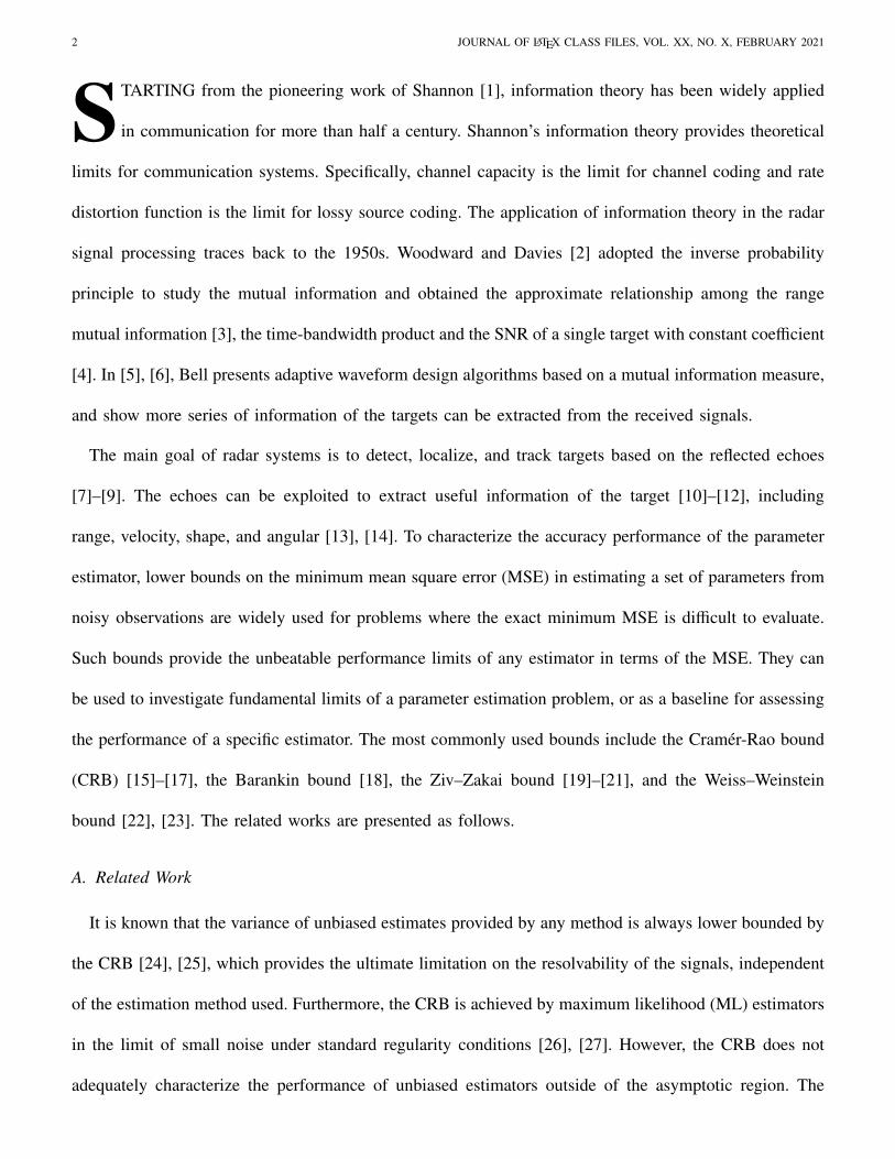
Fig. 3: The RI and the empirical RI of SAP and ML.

In constant amplitudes and complex additive white Gaussian noise scenario, conduct 5000 trials of ML

and SAP estimation. In Fig. 3, the solid line, circle markers and the dotted line with asterisk markers

denote the RI, the empirical RI of SAP and ML, respectively. As can be seen from Fig. 3, the empirical

RI of SAP almost overlaps with RI. The empirical RI of ML is lower than that of SAP in the low to

medium SNR region. Under the low SNR, the empirical RI of ML is slightly higher than EE because of

the edge effect of sinc signal during matched filter, the statistical distribution of ML output value does

not satisfy the uniform distribution.

A numerical simulation is provided to demonstrate the relationship between CRB, EE and the empirical

EE, the CRB, the EE and the empirical EE of MSE in different SNR are shown in Fig 4. It can be found

that EE degenerates to MSE in high SNR region. Also, the EE decreases with increasing SNR and

gradually converges to CRB in the asymptotic region, and provides a tight lower bound for the empirical

EE of MSE.

We have proved that empirical EE of SAP approaches the EE when the snapshot number tends to

infinity. It is of interest to see the relationship between EE and the empirical EE of SAP without infinity

snapshots. To investigate this, we give another numerical study. Fig. 5 shows the EE and the empirical


-10 -5 0 5 10 15 20 25

SNR/dB

10-4

10-3

10-2

10-1

100

101

102

EE

/MS

E

UnachievableEmpirical EE(MSE)EEMSE(MLE)CRB

Fig. 4: EE and MSE of single target with different SNR.

-10 -5 0 5 10 15 20 25

SNR/dB

10-4

10-3

10-2

10-1

100

101

102

EE

EEE-EE(SAP-50)E-EE(SAP-500)

Fig. 5: The EE and the empirical EE of SAP for different snapshots.

EE of SAP estimation for different SNR and snapshot number. circle markers and asterisk markers denote

the empirical EE of SAP estimation of 500 and 50 snapshots, respectively. As can be seen, the deviation

between the empirical EE of SAP and EE is large when the number of snapshots is small. When the

number of snapshots increases, the empirical EE of SAP and EE gradually overlap, which verifies the


Corollary 1.

VII. Conclusion

In this paper, theoretical limits are studied for radar parameter estimation with information theory. range-

scattering information and EE are presented as theoretical limits and SAP is proposed as a limit-achieved

parameter estimator. The closed-form approximation of EE is derived, which indicates that EE degenerates

to MSE in high signal-to-noise (SNR) regime. As a stochastic parameter estimator, the performance of

SAP is entirely decided by the theoretical posteriori PDF of the radar system. Thus, the empirical RI

and the empirical EE of SAP approach the RI and the EE when the snapshot number tends to infinity.

Numerical simulations are conducted to compare the relationship of the EE and the MSE. Results show

that the EE is tighter than the MSE in low and medium SNRs. Also, the achievability of RI and EE is

verified in the simulation.

Appendix

Proof of the approximation of EE

Substitute eq. (36-39) into equation eq. (35)

h(X | Z) = ps log

√2πeβρ

+ (1 − ps) logTρ√

2πe

e12ρ

2+1+ H (ps) (67a)

= log√

2πe + log(

1βρ

)p (Tρ

e12ρ

2+1

)1−ps(

1ps

)ps(

11 − ps

)1−p,

(67b)

= log√

2πe + log(

1ρβps

)p (Tρ

e12ρ

2+1

11 − ps

)1−ps

(67c)

= log√

2πe + log(

1ρβps

)ps

Tρ

e12

2+1

1Tρ2β

Tρ2β+eρ2/2+1

1−ps

(67d)

= log√

2πe + log(

1ρβs

)ps(

1ρβps

)1−ps

(67e)

= log√

2πe + log(

1ρβps

)(67f)

Substitute eq. (67f) into eq. (34), the approximation of EE of single target can be obtained

σ2EE =

(1

ρβps

)2

(68)


Acknowledgment

The authors would like to thank Prof. Xiaofei Zhang and Prof. Fuhui Zhou for the advice on revising

the paper.

References

[1] C. E. Shannon, “A mathematical theory of communication,” Bell Syst. Tech. J., vol. 27, pp. 379–423, 623–656, Jul.–Oct. 1948

[2] P. Woodward and I. Davies, “A theory of radar information,” London, Edinburgh, Dublin Phil. Mag. J. Sci., vol. 41, no. 321, pp.

1001–1017, 1950.

[3] P. Woodward, “Inormation theory and the design of radar receivers,” Proc. IRE, vol. 39, no. 12, pp. 1521–1524, Dec. 1951.

[4] P. M. Woodward, “Probability and Information Theory, With Applications to Radar, ” in International Series of Monographs on

Electronics and Instrumentation, vol. 3. Amsterdam, The Netherlands: Elsevier, 2014.

[5] M. R. Bell, “Information theory and radar: Mutual information and the design and analysis of radar waveforms and systems,” in

California Inst. Technol., Pasadena, CA, USA, 1988

[6] M. R. Bell, “Information theory and radar waveform design,” IEEE Trans. Inf. Theory, vol. 39, no. 5, pp. 1578–1597, 1993

[7] P. Bahl and V. N. Padmanabhan, “RADAR: an in-building RF-based user location and tracking system,” in Nineteenth Annual Joint

Conference of the IEEE Computer and Communications Societies (Cat. No.00CH37064), Tel Aviv, Israel, 2000, pp. 775-784 vol.2.

[8] S. M. Kay and S. L. Marple, “Spectrum analysis—A modern perspective,” Proceedings of the IEEE, vol. 69, no. 11, pp. 1380-1419,

Nov. 1981.

[9] D. Reid, “An algorithm for tracking multiple targets,” IEEE Transactions on Automatic Control, vol. 24, no. 6, pp. 843-854, December

1979.

[10] X. Ye, F. Zhang, Y. Yang, D. Zhu, and S. Pan, “Photonics-based highresolution 3D inverse synthetic aperture radar imaging,” IEEE

Access, vol. 7, pp. 79503–79509, 2019.

[11] E. Fishler, A. Haimovich, R. S. Blum, L. J. Cimini, D. Chizhik and R. A. Valenzuela, “Spatial Diversity in Radars—Models and

Detection Performance,” IEEE Transactions on Signal Processing, vol. 54, no. 3, pp. 823-838, March 2006.

[12] J. Li and P. Stoica, “MIMO Radar with Colocated Antennas,” IEEE Signal Processing Magazine, vol. 24, no. 5, pp. 106-114, Sept.

2007.

[13] V. C. Chen, F. Li, S.-S. Ho and H. Wechsler, “Micro-Doppler effect in radar: phenomenon, model, and simulation study,” IEEE

Transactions on Aerospace and Electronic Systems, vol. 42, no. 1, pp. 2-21, Jan. 2006.

[14] D. Giuli, “Polarization diversity in radars,” Proceedings of the IEEE, vol. 74, no. 2, pp. 245-269, Feb. 1986.

[15] R. A. Fisher, “On the mathematical foundations of theoretical statistics,” Phil. Trans. Roy. Soc., vol. 222, p. 309, 1922.

[16] H. Cramer, Mathematical Methods of Statistics. Princeton, NJ: Princeton Univ. Press, 1946


[17] C. R. Rao, “Information and accuracy attainable in the estimation of statistical parameters,” Bull. Calcutta Math. Soc., vol. 37, pp.

81–91, 1945.

[18] E. W. Barankin, “Locally best unbiased estimates,” Ann. Math. Stat.,vol. 20, pp. 477–501, 1949.

[19] J. Ziv and M. Zakai, “Some lower bounds on signal parameter estimation,” IEEE Trans. Inform. Theory, vol. IT-15, no. 3, pp. 386–391,

May 1969.

[20] L. P. Seidman, “Performance limitations and error calculations for parameter estimation,” Proc. IEEE, vol. 58, pp. 644–652. May 1970.

[21] D. Chazan, M. Zakai, and J. Ziv, “Improved lower bounds on signal parameter estimation,” IEEE Trans. Inform. Theory, vol. IT-21,

no. 1, pp. 90–93, Jan. 1975.

[22] A. J. Weiss, “Fundamental bounds in parameter estimation,” Ph.D. dissertation, Tel-Aviv Univ., Tel-Aviv, Israel, 1985.

[23] E. Weinstein and A. J. Weiss, “A general class of lower bounds in parameter estimation,” IEEE Trans. Inform. Theory, vol. 34, pp.

338–342, Mar. 1988

[24] P. Stoica and A. Nehorai, “MUSIC, maximum likelihood, and Cramer-Rao bound,” IEEE Transactions on Acoustics, Speech, and Signal

Processing, vol. 37, no. 5, pp. 720-741, May 1989.

[25] I. Ziskind and M. Wax, “Maximum likelihood localization of multiple sources by alternating projection,” IEEE Transactions on

Acoustics, Speech, and Signal Processing, vol. 36, no. 10, pp. 1553-1560, Oct. 1988.

[26] J. C. Chen, R. E. Hudson and Kung Yao, “Maximum-likelihood source localization and unknown sensor location estimation for

wideband signals in the near-field,” IEEE Transactions on Signal Processing, vol. 50, no. 8, pp. 1843-1854, Aug. 2002.

[27] M. Pesavento and A. B. Gershman, “Maximum-likelihood direction-of-arrival estimation in the presence of unknown nonuniform noise,”

IEEE Transactions on Signal Processing, vol. 49, no. 7, pp. 1310-1324, July 2001.

[28] S. Xu, D. Xu and H. Luo, “Information theory of detection in radar systems,” in 2017 IEEE International Symposium on Signal

Processing and Information Technology (ISSPIT), Bilbao, 2017, pp. 249-254.

[29] D. Xu, X. Yan, S. Xu, H. Luo, J. Liu and X. Zhang, “Spatial information theory of sensor array and its application in performance

evaluation,” IET Communications, vol. 13, no. 15, pp. 2304-2312, 17 9 2019.

[30] D. Xu, F. ZHANG. Spatial Information Theory, Beijing: Science Press, 2021.

[31] H. Luo, D. Xu, W. Tu and J. Bao, “Closed-Form Asymptotic Approximation of Target’s Range Information in Radar Detection Systems,”

IEEE Access, vol. 8, pp. 105561-105570, 2020.

Documents

A Theoretical Limit of Radar Parameter Estimation