Embed Size (px)
Citation preview

AFRICA GROWTH INITIATIVE
WORKING PAPER 10 | MAY 2013
A THEORETICAL FRAMEWORK FOR KENYA'S CENTRAL BANK MACROECONOMETRIC MODEL
Maureen WereAnne W. KamauMoses M. SicheiMoses Kiptui

Maureen Were is a researcher at the Central Bank
of Kenya, Kenya School of Monetary Studies (KSMS)
Research Centre/Research Department, Nairobi.
Anne W. Kamau is an Africa research fellow at the
Africa Growth Initiative of the Brookings Institution and
at the Central Bank of Kenya, KSMS Research Centre/
Research Department, Nairobi.
Moses M. Sichei is the head of research at the
Commission on Revenue Allocation but was formerly at
the Research Department of the Central Bank of Kenya.
Moses Kiptui is a senior researcher at the KSMS
Research Centre, Central Bank of Kenya.
Abstract
The macroeconometric model was developed as a tool that would aid the Central Bank of Kenya (CBK) in fore-
casting key economic variables in a consistent manner. The economy is modeled in line with economic theory and
structure of Kenya's economy. The monetary sector, which is the main focus of the model, is highly disaggregated
to capture the various relationships that exist between the monetary sector and the real economy. The external,
real and fiscal sectors are not as highly disaggregated and have been incorporated into the model to capture the
transmission channels and the impact of monetary policy. This working paper gives the theoretical foundations
upon which the CBK macroeconometric model is built. The theoretical framework is discussed with the aim of de-
lineating the model’s underlying logical structure and the theoretical base for its core behavioral equations.
Acknowledgements:
The authors are grateful to Njuguna Ndung’u, John Randa and the external model reviewers Alemayehu Geda,
John Weeks and Stephen Karingi for their critical comments on the initial draft of this paper. They would also like to
thank the Africa Growth Initiative external peer reviewer for the valuable comments on the previous version of this
paper. The authors are, however, responsible for any errors and omissions. The views expressed in this paper do
not necessarily represent the official position of the CBK.
For any questions or comments on this paper, you can reach Anne Kamau at [email protected],
Maureen Were at [email protected], Moses Sichei at [email protected], and Moses Kiptui
CONTENTS
1. Introduction . . . . . . . . . . . . . . . . . . . . . . . . . . . . . . . . . . . . . . . . . . . . . . . . . . . . . . . . . . . . . . . . . . . . . . . . . 2
2. An Overview of the Model . . . . . . . . . . . . . . . . . . . . . . . . . . . . . . . . . . . . . . . . . . . . . . . . . . . . . . . . . . . . 4
The Structural Model . . . . . . . . . . . . . . . . . . . . . . . . . . . . . . . . . . . . . . . . . . . . . . . . . . . . . . . . . . . . . . . . 4
Monetary Policy Transmission Mechanisms . . . . . . . . . . . . . . . . . . . . . . . . . . . . . . . . . . . . . . . . . . . . 7
The Details of the Monetary Sector and Its Links with the Other Sectors . . . . . . . . . . . . . . . . . . . 9
3. The Theoretical Base of the Modeled Equations . . . . . . . . . . . . . . . . . . . . . . . . . . . . . . . . . . . . . . . . . 11
The Demand for and Supply of Money . . . . . . . . . . . . . . . . . . . . . . . . . . . . . . . . . . . . . . . . . . . . . . . . 13
Interest Rate Modeling . . . . . . . . . . . . . . . . . . . . . . . . . . . . . . . . . . . . . . . . . . . . . . . . . . . . . . . . . . . . . 15
Inflation Determination . . . . . . . . . . . . . . . . . . . . . . . . . . . . . . . . . . . . . . . . . . . . . . . . . . . . . . . . . . . . . .17
The Consumption Function . . . . . . . . . . . . . . . . . . . . . . . . . . . . . . . . . . . . . . . . . . . . . . . . . . . . . . . . . . 20
The Private Investment Function . . . . . . . . . . . . . . . . . . . . . . . . . . . . . . . . . . . . . . . . . . . . . . . . . . . . . 21
The External Account . . . . . . . . . . . . . . . . . . . . . . . . . . . . . . . . . . . . . . . . . . . . . . . . . . . . . . . . . . . . . . 22
4. Conclusion . . . . . . . . . . . . . . . . . . . . . . . . . . . . . . . . . . . . . . . . . . . . . . . . . . . . . . . . . . . . . . . . . . . . . . . . 27
Appendices . . . . . . . . . . . . . . . . . . . . . . . . . . . . . . . . . . . . . . . . . . . . . . . . . . . . . . . . . . . . . . . . . . . . . . . . . . 28
References . . . . . . . . . . . . . . . . . . . . . . . . . . . . . . . . . . . . . . . . . . . . . . . . . . . . . . . . . . . . . . . . . . . . . . . . . . 30
Endnotes . . . . . . . . . . . . . . . . . . . . . . . . . . . . . . . . . . . . . . . . . . . . . . . . . . . . . . . . . . . . . . . . . . . . . . . . . . . . 35
LIST OF TABLES
Table 1. Summary of Core Sectors and Equations . . . . . . . . . . . . . . . . . . . . . . . . . . . . . . . . . . . . . . . . . . 11
LIST OF FIGURES
Figure 1. Logical Framework and Structure of the Model . . . . . . . . . . . . . . . . . . . . . . . . . . . . . . . . . . . . 4
Figure 2. Submarkets: Quadrants . . . . . . . . . . . . . . . . . . . . . . . . . . . . . . . . . . . . . . . . . . . . . . . . . . . . . . . . 6
Figure 3. Transmission Mechanisms . . . . . . . . . . . . . . . . . . . . . . . . . . . . . . . . . . . . . . . . . . . . . . . . . . . . . . 8
Figure 4. Details of the Monetary Sector and Its Links with Other Sectors . . . . . . . . . . . . . . . . . . . 10

2 GLOBAL ECONOMY AND DEVELOPMENT PROGRAM
A THEORETICAL FRAMEWORK FOR KENYA'S CENTRAL BANK MACROECONOMETRIC MODEL
Maureen WereAnne W. KamauMoses M. SicheiMoses Kiptui
1. INTRODUCTION
This paper presents the theoretical framework for the
Central Bank of Kenya (CBK) macroeconometric model.
In addition, it highlights the theoretical base for the mod-
el’s main behavioral equations. The justification for the
model relates to its usefulness in aiding the policymak-
ing process at the CBK. It is expected that the model
will support the Monetary Policy Committee (MPC) and
Research Department in further understanding how the
economy works through the complex interactions of var-
ious economic agents. The conduct of monetary policy
requires fairly accurate analyses and forecasts backed
up by sound economic theory and a rationale ensuring
that effective monetary policy is formulated and imple-
mented. In this regard, the model will provide consistent
short-term forecasts of key macroeconomic variables
such as economic growth and inflation. In addition, the
model will be helpful in evaluating the impact of various
shocks and policies on the economy. The MPC may
also use the model as an instrument to help in structur-
ing its communication with the public on the rationale
behind its decisions.
This paper is organized as follows. The rest of
Section 1 discusses the type of macro model de-
veloped, Section 2 presents the model’s logical and
theoretical framework and illustrates the linkages be-
tween the monetary submodel and the other blocks
of the model, Section 3 discusses the theoretical
foundations of the model’s behavioral equations, and
Section 4 concludes.
What Type of Model?
Whereas there are different variants of economic mod-
els, two types of macroeconomic models stand out for
macroeconomic policy analysis and forecasting: dy-
namic stochastic general equilibrium (DSGE) models
and macroeconometric models. The choice between
these two categories in a given situation depends on
a number of factors: the purpose for which the model
is needed, the level of detail and complexity required,
and data availability, among other factors. The two
types of models complement each other because no
single model can adequately answer all economic
policy questions or address all needs. DSGE models
are a fairly recent development, whereas macroecono-
metric models date back to 1940s and 1950s, when
the emphasis was on constructing quantitative models
that could help to describe the dynamics observed in
time series economic data.
A THEORETICAL FRAMEWORK FOR KENYA'S CENTRAL BANK MACROECONOMETRIC MODEL 3
Macroeconometric models are most suitable for fore-
casting and policy analysis. Unlike univariate statisti-
cal modeling, macroeconometric models provide a
comprehensive structural view of the entire economy
in a coherent and consistent manner with the level of
detail required for policy analysis. Many central banks
rely on macroeconometric models for economic pro-
jections and analysis, even in cases where they have
other sets of models.1 However, macroeconometric
models came under strong criticism in the 1970s
following the Lucas (1976) and Sargent (1981) find-
ing that the model coefficients were likely not invari-
ant to policy shifts or structural changes. This was
compounded by Sims’s (1980) argument about lack
of clearly identified assumptions that deal with si-
multaneity among macro variables. Despite Lucas’s
critique, many central banks continued to rely on
reduced-form statistical/macro models for forecasting
economic variables (Galì and Gertler 2007).
DSGE models are suitable for analyzing business cycles
and the cyclical effects of monetary policy since they
emphasize the dynamics of the economy. They promise
major benefits for rational policymaking process. DSGE
models are relatively new, having arisen in the 1980s and
1990s as a result of two types of literature that emerged
in response to the shortfalls of traditional macroeconomic
modeling: real business cycle (RBC) theory (Kydland and
Prescott, 1982 and 1990) and New Keynesian theory.
These sought to provide microeconomic foundations
for the Keynesian concepts (Galì and Gertler 2007).
The RBC models assume flexible prices, while the New
Keynesian School assumes price rigidities. These types
of macroeconomic models place greater emphasis on
micro foundations and theoretical coherence.
DSGE models begin by specifying a set of economic
agents (households, firms, governments), each as-
sumed to make optimal choices, in a way that clears
every market. The use of DSGE models at central banks
has become widespread across the globe, especially in
countries that have adopted an inflation-targeting frame-
work. However, a number of limitations have been noted
for these models. First, they tend to perform poorly in
terms of quantitative predictions/projections—since
they are not suited for economic forecasting. Second,
DSGE models are technically more difficult to solve
and analyze, and their use in several central banks,
particularly in developing African countries, is still con-
strained by capacity. Third, they abstract from sectoral
details, making it difficult to study interactions between
individual agents. Fourth, given the strong assump-
tions (e.g., complete markets), critics have argued that
they can be misleading and are unable to describe the
highly nonlinear dynamics of economic fluctuations. The
validity of these assumptions in poor and developing
countries with less developed and incomplete markets
is also questionable. Fifth, they may overstate individual
rationality and foresight and the degree of homogeneity.
To overcome the challenges and shortcomings of relying
on one model, the use of multiple models (i.e., a suite of
models) has also become popular with central banks.
Given the current forecasting needs and the needs of
the MPC, the priority was to first develop a simple mac-
roeconometric model with solid forecasting performance
as part of the overall strategy for developing a suite of
models for the CBK. This was further motivated by the
need to develop a macroeconometric model with a sys-
tematic framework entailing a detailed monetary sector
and how it relates to the other sectors of the economy.
The latter is made possible by the flexibility provided by
the macroeconometric type of models, in terms of their
ease of application and ability to describe economic rela-
tionships based on empirical data and economic theory.
To effectively execute its primary task of formulating and
conducting monetary policy and its secondary role of
promoting economic growth and employment, the CBK
takes cognizance of the structural economic interlinkages
in the economy.
4 GLOBAL ECONOMY AND DEVELOPMENT PROGRAM
2. AN OVERVIEW OF THE MODEL
The Structural Model
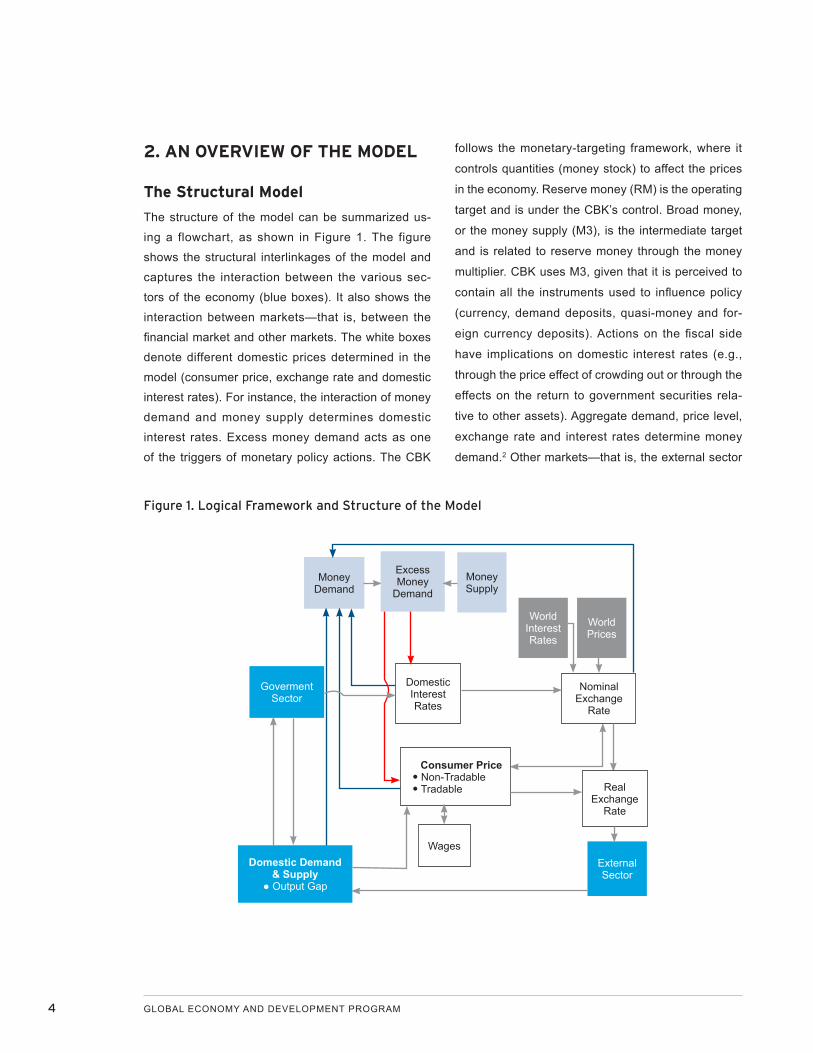
The structure of the model can be summarized us-
ing a flowchart, as shown in Figure 1. The figure
shows the structural interlinkages of the model and
captures the interaction between the various sec-
tors of the economy (blue boxes). It also shows the
interaction between markets—that is, between the
financial market and other markets. The white boxes
denote different domestic prices determined in the
model (consumer price, exchange rate and domestic
interest rates). For instance, the interaction of money
demand and money supply determines domestic
interest rates. Excess money demand acts as one
of the triggers of monetary policy actions. The CBK
follows the monetary-targeting framework, where it
controls quantities (money stock) to affect the prices
in the economy. Reserve money (RM) is the operating
target and is under the CBK’s control. Broad money,
or the money supply (M3), is the intermediate target
and is related to reserve money through the money
multiplier. CBK uses M3, given that it is perceived to
contain all the instruments used to influence policy
(currency, demand deposits, quasi-money and for-
eign currency deposits). Actions on the fiscal side
have implications on domestic interest rates (e.g.,
through the price effect of crowding out or through the
effects on the return to government securities rela-
tive to other assets). Aggregate demand, price level,
exchange rate and interest rates determine money
demand.2 Other markets—that is, the external sector
Figure 1. Logical Framework and Structure of the Model
Goverment Sector
Domestic Demand & Supply
● Output Gap
World Interest Rates
World Prices
External Sector
Domestic Interest Rates
Nominal Exchange
Rate
Consumer Price● Non-Tradable● Tradable
Money Demand
Wages
Real Exchange
Rate
Money Supply
Excess Money
Demand
A THEORETICAL FRAMEWORK FOR KENYA'S CENTRAL BANK MACROECONOMETRIC MODEL 5
and the government/fiscal sector—are represented in
the bright blue boxes.
Unlike the KIPPRA–Treasury Macro Model (KTMM),3
which was designed with a detailed government sector
to meet the government’s needs in the national budget-
ary and planning process, the CBK model has a more
detailed monetary sector tailored to the needs of the
monetary policy process.
The nominal exchange rate is determined in the
foreign exchange market by the differentials be-
tween domestic and world interest rates, as well as
between the domestic price and world prices. For
instance, a rise in domestic interest rates relative to
foreign interest rates will lead to an appreciation of
the local currency. The real exchange rate follows by
definition (i.e., from the nominal exchange rate, the
foreign price and the domestic price level). The (real)
exchange rate has an impact on the exports and im-
ports of goods and services in the external sector.
World price and foreign interest rates are exogenous
(gray boxes).
At the aggregate level, the model closely follows
the aggregate demand (AD)–aggregate supply (AS)
framework. In the short run, income is determined
in the real economy from the demand side, that is,
aggregate demand. Total demand equals the sum of
final consumption expenditures by households, in-
vestment (capital formation), government expenditure
and exports less imports. On the supply side, it is as-
sumed that output is produced in accordance with a
constant elasticity-of-substitution production function
with capital and labor as key inputs. Production leads
to demand for labor and investment goods. Business
enterprises produce goods and services that are sold
in the domestic as well as global markets. The de-
mand for labor and wages is determined in the labor
market. There is a wage-price spiral that can lead to
a vicious cycle in which business owners raise prices
to protect profit margins from rising costs, while wage-
earners push for higher nominal wages to catch up
with rising prices to prevent real wages from falling.
This may be triggered by higher aggregate demand
relative to supply, or the effect of supply shocks such
as international oil price hike. Consumer price is do-
mestically determined through the interaction of AD
and AS, as well as by excess money having an impact
on the price of nontradables. The difference between
actual and potential output is known as the output
gap. Theoretically, this gap is given by the difference
in output between short-run equilibrium, where AD in-
tersects AS, and the long-run AS, which refers to the
natural rate of output.4
The production sector pays net taxes to the govern-
ment. Households sell their labor in the labor market
and receive income in form of remuneration, as well
as dividend payments and transfers from the govern-
ment. They pay taxes and spend their net income
(disposable income) to buy goods and services.
Government spending consists of government ex-
penditure (consumption and investment) and trans-
fers to households.
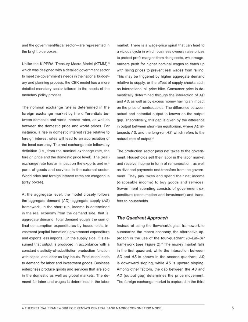
The Quadrant ApproachInstead of using the flowchart/logical framework to
summarize the macro economy, the alternative ap-
proach is the use of the four-quadrant IS–LM–BP
framework (see Figure 2).5 The money market falls
in the first quadrant, while the interaction between
AD and AS is shown in the second quadrant. AD
is downward sloping, while AS is upward sloping.
Among other factors, the gap between the AS and
AD (output gap) determines the price movement.
The foreign exchange market is captured in the third
6 GLOBAL ECONOMY AND DEVELOPMENT PROGRAM
quadrant. A rise in domestic price leads to deprecia-
tion of nominal exchange rate. Given the uncovered
interest parity (UIP) assumption, a policy that leads
to lower interest rates (relative to foreign interest
rates) depreciates the domestic currency. The fourth
quadrant is about the internal and external balance.
The different prices (general domestic price, inter-
est rates and exchange rate) are the main adjusting
components.
Basic SetupQuadrant I: Goods and the Money Market
The IS curve is a combination of points where the
interest rate (r) and output (Y) intersect in the goods
market.6 The goods market is in equilibrium along
those points. It is negatively sloped to indicate that
higher interest rates reduce investment spending,
which in turn reduces aggregate demand and in-
come. The LM curve, conversely, shows a combina-
Figure 2. Submarkets: Quadrants
BOP External and internal balance
E
(f(E))
P(III) (II)
(I)(IV) r
IS
LM1
LM
AD
AD1
AS
r0
r1
45°E1 E0
p0
p1
Y0 Y1 Y
E: Exchange Rate Y: Output
r: Interest Rate
P: Price
A THEORETICAL FRAMEWORK FOR KENYA'S CENTRAL BANK MACROECONOMETRIC MODEL 7
tion of interest rates and output derived in the money
market where money demand equals money supply.
Along this curve, the money market is in equilibrium.
The demand for money is demand for real balances.
The curve is upward sloping, implying that demand
for real balances increases with increases in income
when the money supply is fixed. At the intersection
of the IS and LM curves, the goods and money mar-
kets are in equilibrium.
Quadrant II: Aggregate Demand and Aggregate Supply
The AD and AS curves intersect at a general equi-
librium price level. The AD curve is derived from the
IS–LM equilibrium income at different price levels.
The AS curve reflects the economy’s price adjustment
mechanism. The AS curve is upward sloping in the
short run but vertical in the long run, as it is expected
that equilibrium in the labor market remains the same
at different price levels. The labor market does not
respond to surprises immediately, hence the upward-
sloping AS curve in the short run, due to nominal ri-
gidities such as the sticky wage setup.
Quadrant III: The Foreign Exchange Market
The diagram assumes a small, open economy where
a floating exchange rate regime is followed. In the
foreign exchange market, the endogenous variable in
Quadrant III is the exchange rate, E, whereas the ex-
ogenous variables are the domestic interest rate (rd),
the foreign interest rate ( rf), the expected exchange
rate Ee, domestic prices (Pd) and foreign prices (Pf).
The value of the equilibrium exchange rate is affected
by domestic and foreign rates of return in the market.
Quadrant IV: The Balance of Payments
The internal equilibrium is achieved through Y = C(y) +
I(r) + G + X(e) – Z(e,Y) and the Ms/p = L(r) + k(y). An ap-
preciation of the exchange rate, e, requires a decrease in
government expenditures to have an internal equilibrium.
An appreciation of e worsens the current account balance
position but increases output (Y) through the multiplier ef-
fect. In order to counteract the change in Y, government
spending has to decline. An external balance is attained
through the balance-of-payments (BOP) equilibrium of an
open economy. This may be defined by BOP = X(p,e,y) –
Z (p,e,y) + F(r). The endogenous variable in Quadrant IV
is the balance of payments, and the exogenous variables
are prices (P), the exchange rate (E) and income (output)
(Y). Above the BOP curve, as government spending in-
creases, trade deficits and hence balance-of-payments
deficits arise. As a result, the government must utilize its
foreign reserves to preserve the exchange rate.
The CBK modeling approach closely follows the
Keynesian and monetarist lines of thought, in which
fiscal and monetary policy can be used to raise the
level of output and employment in the economy
in the short run. It contains features of the New
Keynesian economics that emphasize sticky or slug-
gishness in wages and prices to explain why mon-
etary policy affects production activities in the short
run and the new classical models that shed light on
how households and firms make decisions over time.
Combining the different strengths of competing ap-
proaches is expected to yield robust results both in
terms of the theoretical underpinnings and practical
applications of the model.
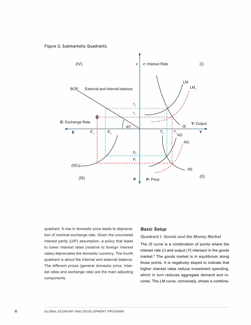
Monetary Policy Transmission Mechanisms
Monetary policy transmission mechanisms describe
how policy-induced changes in the nominal money
stock or the short-term nominal interest rate have an
impact on real variables, such as aggregate output.7
For instance, the MPC changes the Central Bank
Rate (CBR) from time to time to signal the monetary
8 GLOBAL ECONOMY AND DEVELOPMENT PROGRAM
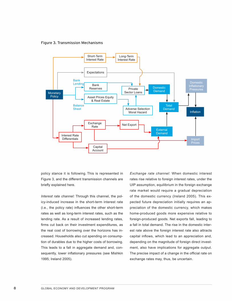
policy stance it is following. This is represented in
Figure 3, and the different transmission channels are
briefly explained here.
Interest rate channel: Through this channel, the pol-
icy-induced increase in the short-term interest rate
(i.e., the policy rate) influences the other short-term
rates as well as long-term interest rates, such as the
lending rate. As a result of increased lending rates,
firms cut back on their investment expenditures, as
the real cost of borrowing over the horizons has in-
creased. Households also cut spending on consump-
tion of durables due to the higher costs of borrowing.
This leads to a fall in aggregate demand and, con-
sequently, lower inflationary pressures (see Mishkin
1995; Ireland 2005).
Exchange rate channel: When domestic interest
rates rise relative to foreign interest rates, under the
UIP assumption, equilibrium in the foreign exchange
rate market would require a gradual depreciation
of the domestic currency (Ireland 2005). This ex-
pected future depreciation initially requires an ap-
preciation of the domestic currency, which makes
home-produced goods more expensive relative to
foreign-produced goods. Net exports fall, leading to
a fall in total demand. The rise in the domestic inter-
est rate above the foreign interest rate also attracts
capital inflows, which lead to an appreciation and,
depending on the magnitude of foreign direct invest-
ment, also have implications for aggregate output.
The precise impact of a change in the official rate on
exchange rates may, thus, be uncertain.
Figure 3. Transmission Mechanisms
Total Demand
Domestic Demand
External Demand
Domestic Inflationary Pressures
Inflation
Import Prices
Monetary Policy
Exchange Rate Net Export
Capital Account
Interest Rate Differentials
Asset Prices Equity & Real Estate
Bank Reserves Private
Sector Loans
Adverse Selection Moral Hazard
Expectations
Short-Term Interest Rate
Long-Term Interest Rate
Bank Lending
Balance Sheet
A THEORETICAL FRAMEWORK FOR KENYA'S CENTRAL BANK MACROECONOMETRIC MODEL 9
The credit channel works in two ways: First, the credit
channel affects the bank lending channel and, sec-
ond, it affects the balance sheet of households and
firms. When the central bank reduces the money
stock by reducing the quantity of reserve money, the
bank’s reserves decline, hence reducing the amount
banks have available for lending out. Conversely, the
reduction in the money stock leads to a worsening of
households’ and firms’ balance sheets through the fall
in asset and equity prices. This reduces the net worth
of the borrowers. Banks then need to screen bor-
rowers in order to avoid adverse selection and then
monitor the borrowers to reduce moral hazard. This
process reduces the amount of loans given by the
banks. Adverse selection and moral hazard are driven
by information imperfections in the market. In both
cases, the effects would reduce domestic demand,
total demand and eventually output. Key assumptions
are that bank loans are firms’ principal sources of
funds, for which few close substitutes exist.
The changes in the policy rate may influence expecta-
tions about the future path of real economic activity and
the confidence with which those expectations are held.
Changes in perception are likely to affect participants
in the financial markets as well as economic agents in
other markets (Bank of England 1999). However, it is
hard to predict the direction in which such effects work.
For instance, a rise in the CBR may be interpreted to
imply that the MPC assumes the economy is likely to
be growing faster than previously thought, which gives
a boost to expectations of future growth and enhances
confidence. But the action can also be interpreted
to imply the need to slow the growth in order to hit
the inflation target, thus yielding expectations of low
future growth and lower confidence. Some previous
studies on monetary policy transmission mechanisms
in Kenya have shown that the bank lending channel
is stronger than all the other channels. The balance
sheet and expectations channels are not modeled in
the model since they are not well developed.
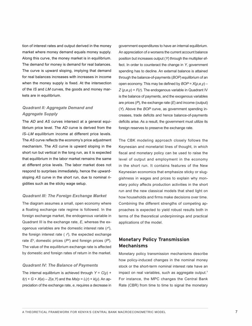
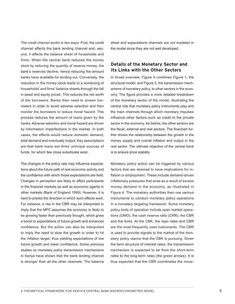
Details of the Monetary Sector and Its Links with the Other Sectors
In broad overview, Figure 4 combines Figure 1, the
structural model, and Figure 3, the transmission mech-
anisms of monetary policy, to other sectors in the econ-
omy. The figure provides a more detailed breakdown
of the monetary sector of the model, illustrating the
central role that monetary policy instruments play and
the main channels through which monetary impulses
influence other factors such as credit to the private
sector in the economy. As before, the other sectors are
the fiscal, external and real sectors. The flowchart fur-
ther shows the relationship between the growth in the
money supply and overall inflation and output in the
real sector. The ultimate objective of the central bank
is to ensure price stability.
Monetary policy action can be triggered by various
factors that are deemed to have implications for in-
flation or employment. These include demand-driven
inflationary pressures that arise as a result of excess
money demand in the economy, as illustrated in
Figure 4. The monetary authorities then use various
instruments to conduct monetary policy operations
in a monetary targeting framework. Some monetary
policy tools of operation include open market opera-
tions (OMO), the cash reserve ratio (CRR), the CBR
and the forex. At the CBK, the repo rates and CBR
are the most frequently used instruments. The CBR
is used to provide signals to the market of the mon-
etary policy stance that the CBK is pursuing. Given
the term structure of interest rates, the transmission
mechanism is expected to be from the short-term
rates to the long-term rates (the green arrows). It is
thus expected that the CBR coordinates the move-
10 GLOBAL ECONOMY AND DEVELOPMENT PROGRAM
ments of short-term rates which eventually affect
the long-term rates such as the lending rate. The
long-term lending rates would affect credit to the
private sector and that will lead to an increase in
money supply. Credit to the private sector also af-
fects investment demand in the real sector. Overall
inflation is primarily influenced by changes in the
prices of imported goods and services, productiv-
ity developments, excesses in money demand and
price expectations. Wage rate fluctuations also play
an important role in price determination.
The money supply is determined via the money
multiplier, mm, and reserve money, RM, and dis-
aggregated by sources—that is, net foreign assets
(NFA), net credit to government (NCG), credit to
the private sector (PSC) and other items net (OIN).
Each is a summation of two components, for CBK
and other depository corporations (ODC). The CBK
components add up to reserve money. The NFA is
determined in the external sector, that is, through
the BOP accounts. NCG is determined in the gov-
ernment sector by the government’s borrowing re-
quirements net of government deposits at the CBK.
This is the same approach that underlies the current
monetary program at the CBK. On the liabilities side,
money demand is composed of currency outside
bank (COB) and deposits. Deposits can be further
disaggregated into demand deposits, quasi-deposits
and foreign currency deposits.
Figure 4. Details of the Monetary Sector and Its Links with Other Sectors
Inflation● Monetary● Imported● Real Sector● Expectations
Real SectorExternal Sector● Exchange Rate● Current Account● Capital Account
Fiscal Sector● Tbill Rate● Revenue● Expenditure
Money Supply
Money Demand
● COB● Deposits
NFA● CBK● ODC
NCG● CBK● ODC
PSC● CBK● ODC
OIN● CBK● ODC
mm
RMTools
● OMO● CRR
● CBR● Forex
Short term rates● Repo● Interbank● Term Auction
POLICY
Excess Money Demand
Long-term rates● Deposit Rates● Lending Rates
A THEORETICAL FRAMEWORK FOR KENYA'S CENTRAL BANK MACROECONOMETRIC MODEL 11
3. THE THEORETICAL BASE OF THE MODELED EQUATIONS
The economy is modeled at the macro level, which is in
line with the modeling approaches employed in these
types of models. In accordance with the underlying
theoretical framework that blends the New Keynesian
and Keynesian traditions, the model allows for nomi-
nal and real inertia as well as the role of aggregate
demand in determining output in the short run. In the
long run, the economic variables gravitate toward their
corresponding supply-side-determined steady states
or equilibrium levels. The model captures the Kenyan
economy as a small, open economy. The key variables
are determined in the model as endogenous variables.
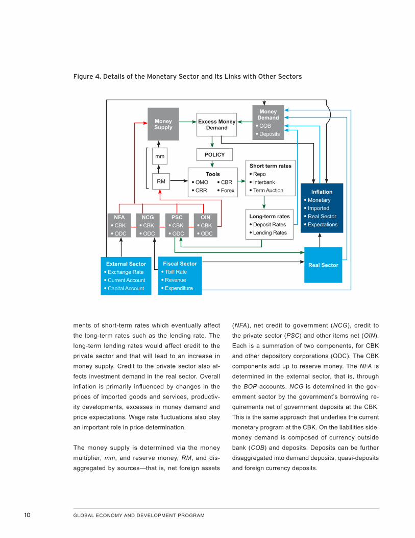
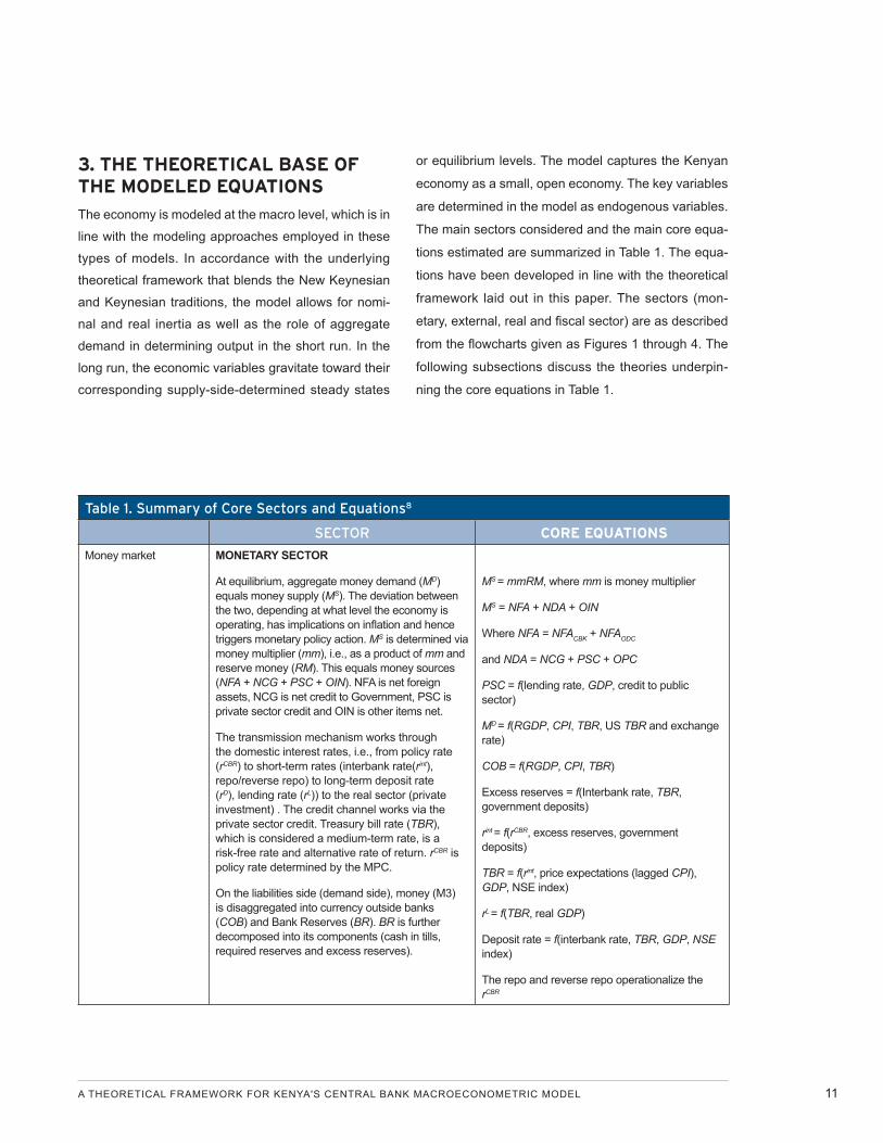
The main sectors considered and the main core equa-
tions estimated are summarized in Table 1. The equa-
tions have been developed in line with the theoretical
framework laid out in this paper. The sectors (mon-
etary, external, real and fiscal sector) are as described
from the flowcharts given as Figures 1 through 4. The
following subsections discuss the theories underpin-
ning the core equations in Table 1.
Table 1. Summary of Core Sectors and Equations8
SECTOR CORE EQUATIONS
Money market MONETARY SECTOR
At equilibrium, aggregate money demand (MD) equals money supply (MS). The deviation between the two, depending at what level the economy is operating, has implications on inflation and hence triggers monetary policy action. MS is determined via money multiplier (mm), i.e., as a product of mm and reserve money (RM). This equals money sources (NFA + NCG + PSC + OIN). NFA is net foreign assets, NCG is net credit to Government, PSC is private sector credit and OIN is other items net.
The transmission mechanism works through the domestic interest rates, i.e., from policy rate (rCBR) to short-term rates (interbank rate(rint), repo/reverse repo) to long-term deposit rate (rD), lending rate (rL)) to the real sector (private investment) . The credit channel works via the private sector credit. Treasury bill rate (TBR), which is considered a medium-term rate, is a risk-free rate and alternative rate of return. rCBR is policy rate determined by the MPC.
On the liabilities side (demand side), money (M3) is disaggregated into currency outside banks (COB) and Bank Reserves (BR). BR is further decomposed into its components (cash in tills, required reserves and excess reserves).
MS = mmRM, where mm is money multiplier
MS = NFA + NDA + OIN
Where NFA = NFACBK + NFAODC
and NDA = NCG + PSC + OPC
PSC = f(lending rate, GDP, credit to public sector)
MD = f(RGDP, CPI, TBR, US TBR and exchange rate)
COB = f(RGDP, CPI, TBR)
Excess reserves = f(Interbank rate, TBR, government deposits)
rint = f(rCBR, excess reserves, government deposits)
TBR = f(rint, price expectations (lagged CPI), GDP, NSE index)
rL = f(TBR, real GDP)
Deposit rate = f(interbank rate, TBR, GDP, NSE index)
The repo and reverse repo operationalize the rCBR
12 GLOBAL ECONOMY AND DEVELOPMENT PROGRAM
SECTOR CORE EQUATIONS
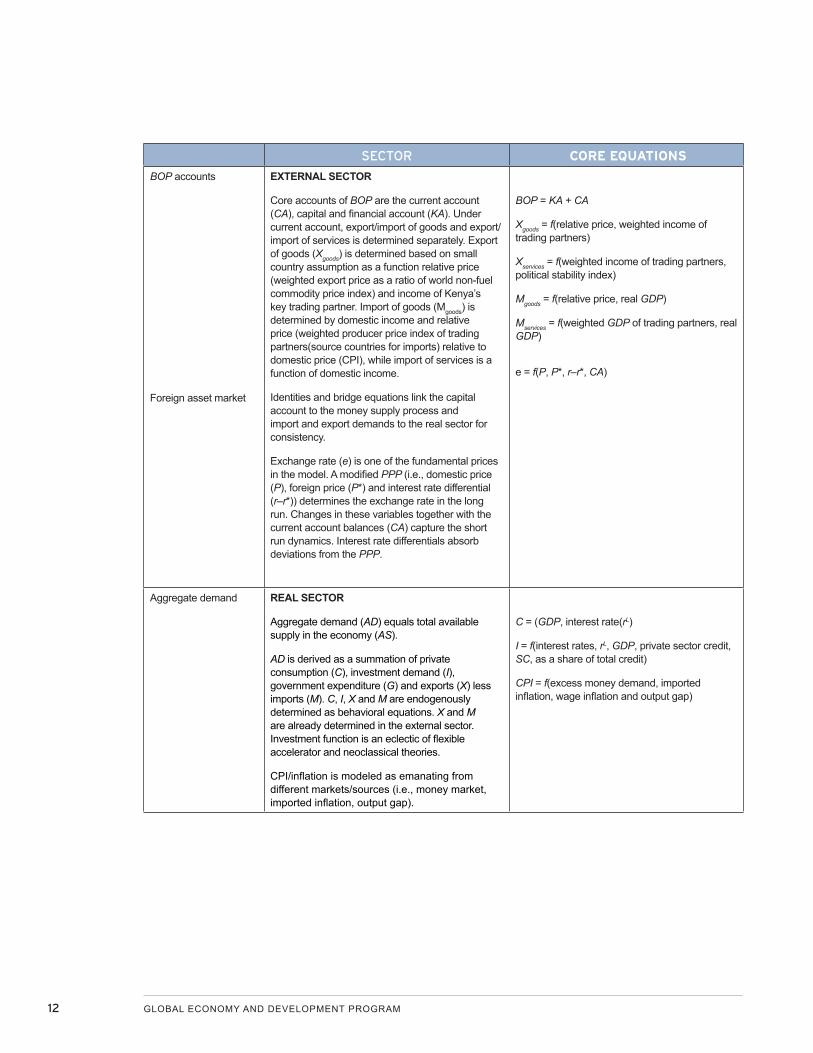
BOP accounts
Foreign asset market
EXTERNAL SECTOR
Core accounts of BOP are the current account (CA), capital and financial account (KA). Under current account, export/import of goods and export/import of services is determined separately. Export of goods (Xgoods) is determined based on small country assumption as a function relative price (weighted export price as a ratio of world non-fuel commodity price index) and income of Kenya’s key trading partner. Import of goods (Mgoods) is determined by domestic income and relative price (weighted producer price index of trading partners(source countries for imports) relative to domestic price (CPI), while import of services is a function of domestic income.
Identities and bridge equations link the capital account to the money supply process and import and export demands to the real sector for consistency.
Exchange rate (e) is one of the fundamental prices in the model. A modified PPP (i.e., domestic price (P), foreign price (P*) and interest rate differential (r–r*)) determines the exchange rate in the long run. Changes in these variables together with the current account balances (CA) capture the short run dynamics. Interest rate differentials absorb deviations from the PPP.
BOP = KA + CA
Xgoods = f(relative price, weighted income of trading partners)
Xservices = f(weighted income of trading partners, political stability index)
Mgoods = f(relative price, real GDP)
Mservices = f(weighted GDP of trading partners, real GDP)
e = f(P, P*, r–r*, CA)
Aggregate demand REAL SECTOR
Aggregate demand (AD) equals total available supply in the economy (AS).
AD is derived as a summation of private consumption (C), investment demand (I), government expenditure (G) and exports (X) less imports (M). C, I, X and M are endogenously determined as behavioral equations. X and M are already determined in the external sector. Investment function is an eclectic of flexible accelerator and neoclassical theories.
CPI/inflation is modeled as emanating from different markets/sources (i.e., money market, imported inflation, output gap).
C = (GDP, interest rate(rL)
I = f(interest rates, rL, GDP, private sector credit, SC, as a share of total credit)
CPI = f(excess money demand, imported inflation, wage inflation and output gap)
A THEORETICAL FRAMEWORK FOR KENYA'S CENTRAL BANK MACROECONOMETRIC MODEL 13
SECTOR CORE EQUATIONS
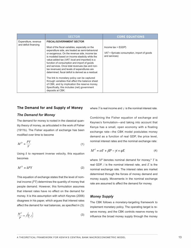
Expenditure, revenue and deficit financing
FISCAL/GOVERNMENT SECTOR
Most of the fiscal variables, especially on the expenditure side, are treated as semi-behavioral or exogenous. On the revenue side, income tax is modeled based on income elasticity while the value-added tax (VAT; local and imported) is a function of consumption and import of goods and services. Once total revenues (tax and non-tax revenues) and levels of expenditures are determined, fiscal deficit is derived as a residual.
The link to monetary policy can be captured through variables that affect the balance sheet of CBK, and by implication the reserve money. Specifically, this includes (net) government deposits at CBK.
Income tax = f(GDP)
VAT = f(private consumption, import of goods and services)
The Demand for and Supply of Money
The Demand for Money The demand for money is rooted in the classical quan-
tity theory of money, as articulated in the work of Fisher
(1911b). The Fisher equation of exchange has been
modified over time to become
VPYM D (1)
Using k to represent inverse velocity, this equation
becomes
kPYM D (2)
This equation of exchange states that the level of nom-
inal income (PY) determines the quantity of money that
people demand. However, this formulation assumes
that interest rates have no effect on the demand for
money. It is this assumption with which Keynes (2006)
disagrees in his paper, which argues that interest rates
affect the demand for real balances, as specified in (3):
iYfP
M d
, (3)
where Y is real income and i is the nominal interest rate.
Combining the Fisher equation of exchange and
Keynes’s formulation—and taking into account that
Kenya has a small, open economy with a floating
exchange rate—the CBK model postulates money
demand as a function of real GDP, the price level,
nominal interest rates and the nominal exchange rate:
EiPYM d (4)
where M d denotes nominal demand for money,9 Y is
real GDP, i is the nominal interest rate, and E is the
nominal exchange rate. The interest rates are market
determined through the forces of money demand and
money supply. Movements in the nominal exchange
rate are assumed to affect the demand for money.
Money SupplyThe CBK follows a monetary-targeting framework to
implement monetary policy. The operating target is re-
serve money, and the CBK controls reserve money to
influence the broad money supply through the money
14 GLOBAL ECONOMY AND DEVELOPMENT PROGRAM
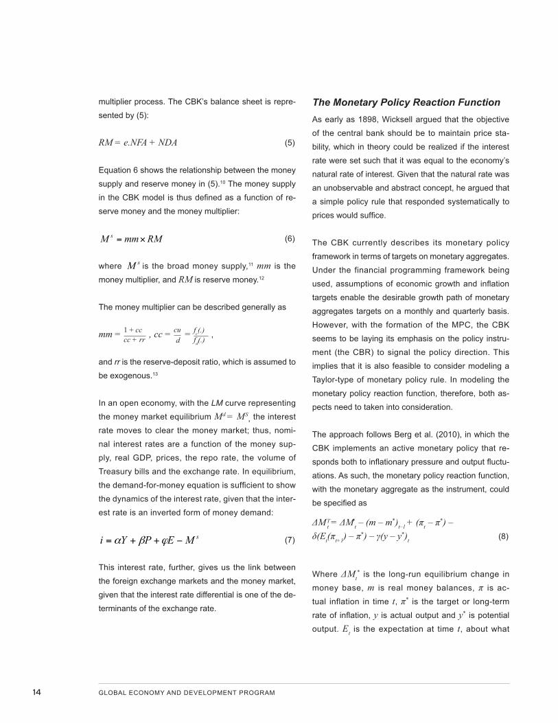
multiplier process. The CBK’s balance sheet is repre-
sented by (5):
RM = e.NFA + NDA (5)
Equation 6 shows the relationship between the money
supply and reserve money in (5).10 The money supply
in the CBK model is thus defined as a function of re-
serve money and the money multiplier:
RMmmM s (6)
where sM is the broad money supply,11 mm is the
money multiplier, and RM is reserve money.12
The money multiplier can be described generally as
mm = 1 + cccc + rr , cc = cu
d = fc(.)
fd(.) ,
and rr is the reserve-deposit ratio, which is assumed to
be exogenous.13
In an open economy, with the LM curve representing
the money market equilibrium Md = MS, the interest
rate moves to clear the money market; thus, nomi-
nal interest rates are a function of the money sup-
ply, real GDP, prices, the repo rate, the volume of
Treasury bills and the exchange rate. In equilibrium,
the demand-for-money equation is sufficient to show
the dynamics of the interest rate, given that the inter-
est rate is an inverted form of money demand:
sMEPYi (7)
This interest rate, further, gives us the link between
the foreign exchange markets and the money market,
given that the interest rate differential is one of the de-
terminants of the exchange rate.
The Monetary Policy Reaction Function As early as 1898, Wicksell argued that the objective
of the central bank should be to maintain price sta-
bility, which in theory could be realized if the interest
rate were set such that it was equal to the economy’s
natural rate of interest. Given that the natural rate was
an unobservable and abstract concept, he argued that
a simple policy rule that responded systematically to
prices would suffice.
The CBK currently describes its monetary policy
framework in terms of targets on monetary aggregates.
Under the financial programming framework being
used, assumptions of economic growth and inflation
targets enable the desirable growth path of monetary
aggregates targets on a monthly and quarterly basis.
However, with the formation of the MPC, the CBK
seems to be laying its emphasis on the policy instru-
ment (the CBR) to signal the policy direction. This
implies that it is also feasible to consider modeling a
Taylor-type of monetary policy rule. In modeling the
monetary policy reaction function, therefore, both as-
pects need to taken into consideration.
The approach follows Berg et al. (2010), in which the
CBK implements an active monetary policy that re-
sponds both to inflationary pressure and output fluctu-
ations. As such, the monetary policy reaction function,
with the monetary aggregate as the instrument, could
be specified as
T *ΔM t = ΔM t – (m – m*)t–1 + (πt – π*) – δ(Et(πt+1) – π*) – γ(y – y*)t (8)
Where ΔMt* is the long-run equilibrium change in
money base, m is real money balances, π is ac-
tual inflation in time t, π* is the target or long-term
rate of inflation, y is actual output and y* is potential
output. Et is the expectation at time t, about what
A THEORETICAL FRAMEWORK FOR KENYA'S CENTRAL BANK MACROECONOMETRIC MODEL 15
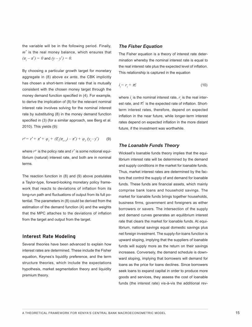
the variable will be in the following period. Finally,
m* is the real money balance, which ensures that
(πt – π*) = 0 and (y – y*) = 0.
By choosing a particular growth target for monetary
aggregate in (8) above ex ante, the CBK implicitly
has chosen a short-term interest rate that is mutually
consistent with the chosen money target through the
money demand function specified in (4). For example,
to derive the implication of (8) for the relevant nominal
interest rate involves solving for the nominal interest
rate by substituting (8) in the money demand function
specified in (3) (for a similar approach, see Berg et al.
2010). This yields (9):
rp = r* + π* + φ1 + (Et(πt+1) – π*) + φ2 (yt – y*) (9)
where rp is the policy rate and r* is some notional equi-
librium (natural) interest rate, and both are in nominal
terms.
The reaction function in (8) and (9) above postulates
a Taylor-type, forward-looking monetary policy frame-
work that reacts to deviations of inflation from its
long-run path and fluctuations of output from its full po-
tential. The parameters in (8) could be derived from the
estimation of the demand function (4) and the weights
that the MPC attaches to the deviations of inflation
from the target and output from the target.
Interest Rate Modeling
Several theories have been advanced to explain how
interest rates are determined. These include the Fisher
equation, Keynes’s liquidity preference, and the term
structure theories, which include the expectations
hypothesis, market segmentation theory and liquidity
premium theory.
The Fisher EquationThe Fisher equation is a theory of interest rate deter-
mination whereby the nominal interest rate is equal to
the real interest rate plus the expected level of inflation.
This relationship is captured in the equation
it = rt + πe (10)
where it is the nominal interest rate, rt is the real inter-
est rate, and πe is the expected rate of inflation. Short-
term interest rates, therefore, depend on expected
inflation in the near future, while longer-term interest
rates depend on expected inflation in the more distant
future, if the investment was worthwhile.
The Loanable Funds Theory Wicksell’s loanable funds theory implies that the equi-
librium interest rate will be determined by the demand
and supply conditions in the market for loanable funds.
Thus, market interest rates are determined by the fac-
tors that control the supply of and demand for loanable
funds. These funds are financial assets, which mainly
comprise bank loans and household savings. The
market for loanable funds brings together households,
business firms, government and foreigners as either
borrowers or savers. The intersection of the supply
and demand curves generates an equilibrium interest
rate that clears the market for loanable funds. At equi-
librium, national savings equal domestic savings plus
net foreign investment. The supply-for-loans function is
upward sloping, implying that the suppliers of loanable
funds will supply more as the return on their savings
increases. Conversely, the demand schedule is down-
ward sloping, implying that borrowers will demand for
loans as the price for loans declines. Since borrowers
seek loans to expand capital in order to produce more
goods and services, they assess the cost of loanable
funds (the interest rate) vis-à-vis the additional rev-
16 GLOBAL ECONOMY AND DEVELOPMENT PROGRAM
enue from the additional capital (the rate of return on
capital). Hence, borrowers’ demand for additional capi-
tal (loans to expand capital) will continue to grow so
long as the return on the borrowed funds exceeds the
interest rate on the borrowed funds, and will stop at the
point where the interest rate equals the rate of return
on capital. That is, a company’s demand continues to
grow so long as the rate of return on its capital contin-
ues to increase.
Keynes’s Liquidity PreferenceAccording to the liquidity preference theory, the mar-
ket rate of interest is determined by the demand for
and supply of money balances. This theory states
that people demand money for transactions, as a
precaution and for speculative purposes. The trans-
action demand and precautionary demand for money
increase with income, while the speculative demand
is inversely related to interest rates because of the
forgone interest. The supply of money is determined
by the monetary authority (i.e., the central bank), by
the lending of commercial banks and by the public
preference for holding cash.
This is consistent with the liquidity preference theory
of the term structure of interest rates, whereby inter-
est rates are expected to increase as the maturity
profile of securities increases. This is so because the
longer the maturity, the greater is the uncertainty;
and therefore the premium demanded by investors
to part with cash increases as the maturity profile in-
creases. The expectation, therefore, is that forward
rates should offer a premium over expected future
spot rates since those who are risk-averse demand
a premium for securities with longer-term maturities.
A premium is offered by way of greater forward rates
in order to attract investors to longer-term securities.
Consequently, current interest rates reflect expected
inflation rates, income (GDP) and expected money
supply changes:
i = f(GDP, ms, πe) (11)
The Expectations Theory of the Term StructureAccording to expectations theory, long-term interest
rates are averages of expected future short-term inter-
est rates. Thus, a return on a two-year security should
be equal to the anticipated return from investing in two
consecutive one-year securities:
(1 + R2)2 = (1 + R1)(t+1r1) (12)
where R1 and R2 are, respectively, the known annual-
ized rate on one-year and two-year securities and t+1r1
is one-year interest rate that is anticipated in time t+1.
This can be generalized to n periods, so that an “n”-
year security should offer a return that is equal to the
expected return from investing in n consecutive one-
year securities:
(1 + Rn)n = (1 + R1) (t+1r1) (t+2r1)…………(t+nr1) (13)
where t+nr1 is the one-year interest rate that is antici-
pated as of time t+n and Rn is the known annualized
rate on an “n”-year security.
Interest Rate Modeling for the CBK Macroeconometric ModelThe interest rate equation for the CBK model incorpo-
rates all the aspects of the three theories discussed
above. In addition, based on the MPC’s market sur-
vey—which indicates that lenders take into account
short-term rates (interbank, Treasury bill rates) in the
lending rate—the interest rate equation is modeled as
A THEORETICAL FRAMEWORK FOR KENYA'S CENTRAL BANK MACROECONOMETRIC MODEL 17
q
j
r
kt
s
l
v
mmtmltlktkjtjit
p
iiititititt TbillrDeprCPIRGDPiTbillrDeprCPIRGDPii
0 0 0 0154321
q
j
r
kt
s
l
v
mmtmltlktkjtjit
p
iiititititt TbillrDeprCPIRGDPiTbillrDeprCPIRGDPii
0 0 0 0154321
q
j
r
kt
s
l
v
mmtmltlktkjtjit
p
iiititititt TbillrDeprCPIRGDPiTbillrDeprCPIRGDPii
0 0 0 0154321 (14)
Where i is the overall weighted average lending rate
of commercial banks; RGDP is real output; CPI is
the consumer price index; Tbill is the average 91-day
Treasury bill rate and Depr is the overall weighted av-
erage deposit rate of commercial banks.
Inflation Determination
Inflation in open economies results from different dis-
equilibria in many markets—specifically, the domestic
money market, external/foreign markets and the labor
market. Thus we recognize that inflation emanates
from three main sources in the CBK model: excess
money supply, foreign prices and cost push factors.
The Monetarist Model of Inflation
The monetarist views inflation as “always and every-
where a monetary phenomenon” (Friedman 1963).
Further, macroeconomic theory proposes that growing
the money supply in excess of real growth causes infla-
tion. This is also the result from the Harberger (1963)
model, which assumes “that prices adjust to excess
money supply in the money market.” It is on the basis of
this assumption that it is possible to invert the real money
demand equation as a price equation in equation 15:
P = f (M, y, i) (15)
where P is the price level, M is the nominal money
supply, y is real GDP, and i is the nominal interest rate.
On the basis of the Harberger model, which makes it
possible to invert the real money balances function to
become a price equation, we obtain
tttt iyMP 321 (16)
Imported InflationModeling imported inflation follows either the purchas-
ing power parity (PPP) or the UIP condition or a com-
bination of the two.
The theory of PPP requires that nominal exchange
rates move to equalize the price of goods and services
across countries. There are two versions of the PPP:
the absolute version (law of one price) and the rela-
tive version. Following the relative PPP theory, infla-
tion rate differentials between two countries or regions
are offset through inverse changes in the nominal ex-
change rate so that purchasing power ratio between
the two remains constant.
The relative PPP is formally expressed as
*ttt ppce (17)
where tp is the log of the domestic price level, *tp is
the log of the foreign price level, te is the log of the spot
nominal effective exchange rate (i.e., the Kenya shillings
price of a unit of foreign currency) and c is a constant
representing the permanent deviation from absolute
PPP due to productivity differentials and other factors.
Since goods arbitrage is slow, PPP represents a
longer-term relationship than equation 17 suggests.
There are a number of factors that could drive the
exchange rate temporarily away from the PPP. These
include commodity prices, different interest rate struc-
tures, relative growth differentials and speculative price
18 GLOBAL ECONOMY AND DEVELOPMENT PROGRAM
movements. Whenever there is a deviation from PPP, it
is expected that the exchange rate will move smoothly
toward restoring relative PPP, as shown in equation 18:
Δet+1 = α[pt – pt* – et– c] (18)
where 10 .
Conversely, the theory of UIP requires that if interest
rates in Kenya are higher than similar interest rates in
the United States, then investors will have an incentive
to purchase Kenyan assets. UIP can be expressed al-
gebraically as
tmt
mttmtt uiieeE
* (19)
where =tE is the expectation on the basis of all infor-
mation available at time t, =mti is the yield on domestic
assets with maturity m at time t, =*mti is an equivalent
foreign interest rate, and =tu is the risk premium asso-
ciated with holding Kenya shilling assets.
The available evidence shows that PPP and UIP have
been rejected individually due to a failure to recognize
the systematic relationship between the two condi-
tions. Following Choy (2000) we combine PPP and
UIP as follows.
Assuming rational expectations, equation 18 can be
rewritten as
Et(et+m ) – et = α[pt – pt* – et– c] (20)
The exchange rate expectations also feature in the
UIP condition in equation 19. If we assume that PPP
forms the basis of the expectations in the UIP as-
sumption, we can substitute equation 20 for expecta-
tions in equation 19;
α[pt – pt* – et– c] = it
m – itm* + ut (21)
Rearranging,
01 ** kiippe mt
mtttt (22)
where uck
In the real world, the relationship in equation 22 is not
deterministic. Speculative activity or commodity price
movements could, for instance, lead to a sustained
and significant deviation from equation 22. Thus equa-
tion 22 can be viewed as an equilibrium condition
toward which prices, interest rates and the exchange
rate tend to move in the long run—that is, prices, inter-
est rates and the exchange rate are cointegrated:
)0(~6*
15
14
14
*
13
12
11 Iiiippe
k
mt
mt
mtttt
(23)
Equation 21 can be further relaxed in three ways to
take into consideration the weak form of PPP and UIP.
First, we are not concerned with meeting the actual
magnitudes stated in equation 22 but rather the direc-
tion. Second, the analysis takes into consideration the
small country assumption, whereby external variables
are treated as weakly exogenous. Finally, crude oil
prices are added as an additional variable given the
fact that Kenya is a net importer of oil.
Wages and InflationThere are three different levels of wage formation in
Kenya: unionized, competitive and administered. This
implies that the observed wage is a function of com-
petitive, administered and bargained wages, which can
be explained by different theories of unemployment.
First is the efficiency wage theory, in which there is
a cost as well as a benefit to the firm of paying lower
A THEORETICAL FRAMEWORK FOR KENYA'S CENTRAL BANK MACROECONOMETRIC MODEL 19
wages (e.g., the model of Shapiro and Stiglitz 1984).
The second are the contracting models (explicit and
implicit contracts). Under implicit contracts, there is
a long-term relationship between firms and workers.
Firms do not hire workers afresh every period but,
rather, many jobs involve long-term attachments and
considerable firm-specific skills acquired by workers.
This model implies that wages do not have to adjust
to clear the labor market each period. Thus, workers
are content to stay in their current jobs as long as the
salary they expect to obtain is preferable to the outside
job opportunity. This model is applicable to some labor,
especially in central and local government, as well as
some private firms.
The third model is the insider-outsider model, which
assumes that there are two groups of potential work-
ers. The first group is the insiders who have some con-
nection with the firm at the time of bargaining, and thus
the wage contract takes their interest into account. The
second group are the outsiders who have no initial
connection with the firm but who may be hired after the
contract is set. This model assumes that the outsiders’
and insiders’ wages are linked.
The fourth model is the bargaining theory of wages,
which holds that wages, work hours and conditions are
dependent on the relative bargaining strengths of the
parties involved in the agreement. The details of wage
bargaining are presented by Huizinga et al. (2001)
(see appendix 2).
The different bargaining structures show different re-
lationships between an increase in the real consump-
tion wage and the real product wage (see Flanagan,
Moene and Wallerstein 1993). Under markup pricing,
with increases in wages in one sector and not others,
output price will increase but the impact on the con-
sumer price will be smaller. Conversely, if bargaining is
centralized so that wages rise in most of the economy,
then the increase in real product wages will be similar
to the increase in the consumption wage. The price
wedge also depends on the extent of product mar-
ket competition. If a particular industry is exposed to
intense foreign competition, product prices cannot
be increased as much, even though domestic wages
rise. However, since the consumption basket contains
imported goods and services, foreign trade and the
domestic service sector will also influence the price of
real consumption wages.
If a nationwide wage increase initially affects a highly
exposed industry with output prices already at or
above the competitive foreign trade levels, the indus-
try has three options. First, it can reduce employment
until the marginal cost equals the competitive price.
Second, it can increase labor productivity. Or third, it
can close down the industry with regard to labor pro-
ductivity. It is important to make a distinction between a
rise in labor productivity due to technological progress
or an elimination of previous excess capacity.
In Kenya, there are formal collective wage bargaining
agreements, and there are also administered minimum
wage guidelines. The government legislates minimum
wages through wage guidelines, introduced in 1973,
to guide the Industrial Court in adjudicating trade dis-
putes. The government made some changes in 1994.
Wage guidelines were liberalized, allowing workers
and employers greater freedom in wage negotiations
for maximum compensation for rises in the cost of
living. The wage guidelines give consideration to pro-
ductivity and performance in addition to changes in the
cost of living as reflected by the inflation rate.
The empirical equation for testing is in the form
tttytctct rarerappaaprpw ,332,,10, (24)
20 GLOBAL ECONOMY AND DEVELOPMENT PROGRAM
where prpw tct , is the negative of the markup; tytc pp ,, is the price wedge (i.e., the ratio of the
CPI to the GDP deflator; trer is the real exchange
rate; and =tr is the real interest rate. The expectation
is that 0 ≤ a1 ≤ 1 and measures the bargaining power
of the labor unions; a2 ≥ 0 (i.e., lower markup following
exchange rate appreciation; Phelps 1994); and a3 ≥ 0
(i.e., higher markup following an increase in real inter-
est rates).
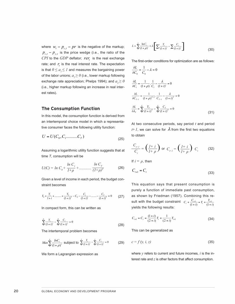
The Consumption Function
In this model, the consumption function is derived from
an intertemporal choice model in which a representa-
tive consumer faces the following utility function:
)..........,( 10 TCCCUU = (25)
Assuming a logarithmic utility function suggests that at
time T, consumption will be
U(C) = ln C0 + ln C1
1+ρ +............ ln CT
(1+ρ)T (26)
Given a level of income in each period, the budget con-
straint becomes
0)1(
.......)1()1(
.........1 1
10
10
T
TT
T
iC
iCC
iY
iYY (27)
In compact form, this can be written as
T
tt
T
tt
iC
iY
000
)1()1( (28)
The intertemporal problem becomes
T
ttInC
Max0 )1(
subject to
T
tt
T
tt
iC
iY
000
)1()1( (29)
We form a Lagrangian expression as
T
tt
tt
T
tt
iC
iYC
L0
0 )1()1()1(ln
[
T
tt
tt
T
tt
iC
iYC
L0
0 )1()1()1(ln
] (30)
The first-order conditions for optimization are as follows:
01
00
CC
L
0)1(
1.)1(
1
11
tiCCL
T T
TT
TT
T
TT
TT
iC
iYL
iCCL
0 0
11
1
0)1()1(
0)1(
1.)1(
1
T T
TT
TT
T
TT
TT
iC
iYL
iCCL
0 0
11
1
0)1()1(
0)1(
1.)1(
1
(31)
At two consecutive periods, say period t and period
t+1, we can solve for from the first two equations
to obtain
Ct+1
Ct = (1+ i
1+ ρ ) or Ct+1 = (1+ i1+ ρ ) Ct
(32)
If i = ρ, then
tt CC =+1 (33)
This equation says that present consumption is
purely a function of immediate past consumption,
as shown by Friedman (1957). Combining this re-
sult with the budget constraint )1()1(
11
iYY
iCC t
tt
t ++=
++ ++
yields the following results:
11 )2(1
)2()1(
++ ++
++
== tttt Yi
YiiCC (34)
This can be generalized as
c = f (y, i, z) (35)
where y refers to current and future incomes, i is the in-
terest rate and z is other factors that affect consumption.
A THEORETICAL FRAMEWORK FOR KENYA'S CENTRAL BANK MACROECONOMETRIC MODEL 21
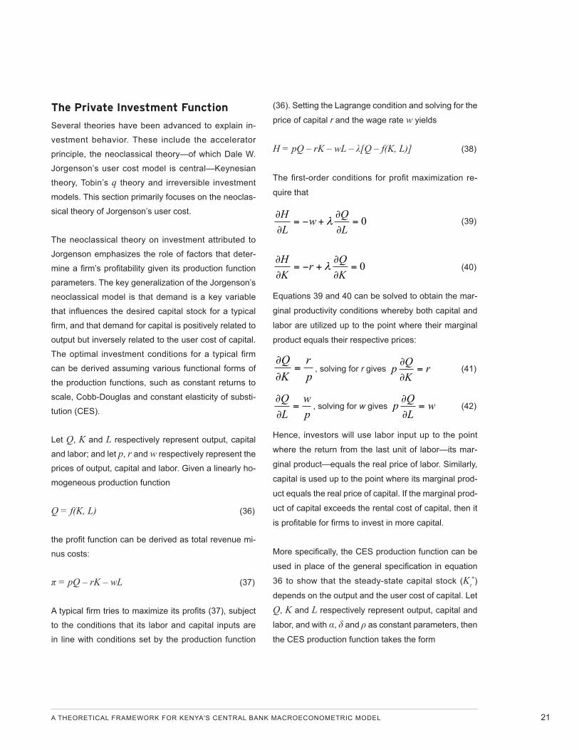
The Private Investment Function
Several theories have been advanced to explain in-
vestment behavior. These include the accelerator
principle, the neoclassical theory—of which Dale W.
Jorgenson’s user cost model is central—Keynesian
theory, Tobin’s q theory and irreversible investment
models. This section primarily focuses on the neoclas-
sical theory of Jorgenson’s user cost.
The neoclassical theory on investment attributed to
Jorgenson emphasizes the role of factors that deter-
mine a firm’s profitability given its production function
parameters. The key generalization of the Jorgenson’s
neoclassical model is that demand is a key variable
that influences the desired capital stock for a typical
firm, and that demand for capital is positively related to
output but inversely related to the user cost of capital.
The optimal investment conditions for a typical firm
can be derived assuming various functional forms of
the production functions, such as constant returns to
scale, Cobb-Douglas and constant elasticity of substi-
tution (CES).
Let Q, K and L respectively represent output, capital
and labor; and let p, r and w respectively represent the
prices of output, capital and labor. Given a linearly ho-
mogeneous production function
Q = f(K, L) (36)
the profit function can be derived as total revenue mi-
nus costs:
π = pQ – rK – wL (37)
A typical firm tries to maximize its profits (37), subject
to the conditions that its labor and capital inputs are
in line with conditions set by the production function
(36). Setting the Lagrange condition and solving for the
price of capital r and the wage rate w yields
H = pQ – rK – wL – λ[Q – f(K, L)] (38)
The first-order conditions for profit maximization re-
quire that
0
LQw
LH
(39)
0
KQr
KH
(40)
Equations 39 and 40 can be solved to obtain the mar-
ginal productivity conditions whereby both capital and
labor are utilized up to the point where their marginal
product equals their respective prices:
pr
KQ
, solving for r gives r
KQp
(41)
pw
LQ
, solving for w gives w
LQp
(42)
Hence, investors will use labor input up to the point
where the return from the last unit of labor—its mar-
ginal product—equals the real price of labor. Similarly,
capital is used up to the point where its marginal prod-
uct equals the real price of capital. If the marginal prod-
uct of capital exceeds the rental cost of capital, then it
is profitable for firms to invest in more capital.
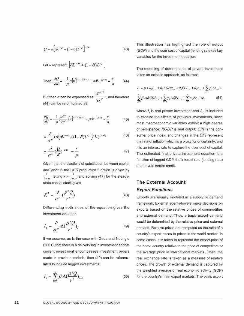
More specifically, the CES production function can be
used in place of the general specification in equation
36 to show that the steady-state capital stock (Kt*)
depends on the output and the user cost of capital. Let
Q, K and L respectively represent output, capital and
labor, and with α, δ and ρ as constant parameters, then
the CES production function takes the form
22 GLOBAL ECONOMY AND DEVELOPMENT PROGRAM
/1)1( LKQ (43)
Let u represent LK )1(
Then,
rKuKQ
)1()1)(/1(1 (44)
But then α can be expressed as
1
, and therefore
(44) can be reformulated as
rKuKQ
)1()1)(/1(1
)(1
(45)
)1()/)1((
KLK (46)
rKQ
)1()( (47)
Given that the elasticity of substitution between capital
and labor in the CES production function is given by
11
, letting x = 11
and solving (47) for the steady-
state capital stock gives
)(*x
x
rQK
(48)
Differencing both sides of the equation gives the
investment equation
tx
x
t rQI )(
(49)
If we assume, as is the case with Geda and Ndung’u
(2001), that there is a delivery lag in investment so that
current investment encompasses investment orders
made in previous periods, then (49) can be reformu-
lated to include lagged investments:
itx
xn
iit r
QI
)(0
(50)
This illustration has highlighted the role of output
(GDP) and the user cost of capital (lending rate) as key
variables for the investment equation.
The modeling of determinants of private investment
takes an eclectic approach, as follows:
(51)
where It is real private investment and It–i is included
to capture the effects of previous investments, since
most macroeconomic variables exhibit a high degree
of persistence; RGDP is real output; CPI is the con-
sumer price index, and changes in the CPI represent
the rate of inflation which is a proxy for uncertainty; and
r is an interest rate to capture the user cost of capital.
The estimated final private investment equation is a
function of lagged GDP, the interest rate (lending rate)
and private sector credit.
The External Account
Export Functions Exports are usually modeled in a supply or demand
framework. External agents/buyers make decisions on
exports based on the relative prices of commodities
and external demand. Thus, a basic export demand
would be determined by the relative price and external
demand. Relative prices are computed as the ratio of a
country's export prices to prices in the world market. In
some cases, it is taken to represent the export price of
the home country relative to the price of competitors or
the average price in international markets. Often, the
real exchange rate is taken as a measure of relative
prices. The growth of external demand is captured by
the weighted average of real economic activity (GDP)
for the country’s main export markets. The basic export
q
j
r
kt
s
lltlktkjtjit
p
iiititititt rCPIRGDPIrCPIRGDPII
0 0 014321
q
j
r
kt
s
lltlktkjtjit
p
iiititititt rCPIRGDPIrCPIRGDPII
0 0 014321
A THEORETICAL FRAMEWORK FOR KENYA'S CENTRAL BANK MACROECONOMETRIC MODEL 23
supply specification is formulated on the basis of the as-
sumption that producers base their production decisions
on, one, domestic capacity and, two, prices, which de-
termine the relative profitability of producing for the ex-
port market vis-à-vis producing other competing goods.
The three measures that have been primarily used as
proxies for domestic capacity are Trend of gross do-mestic product, y*, a sectoral production index, or ca-pacity utilization index, normally defined as deviations from trend output.
Measures of price effects, which include the real exchange rate (RER) as an indicator of the relative profitability of producing tradable versus nontradables goods; and the ratio of export prices to the prices of other tradable goods, as an indicator of the profit-ability of exporting specific export goods relative to other traded goods. Relative profitability in this case is measured by the ratio of export prices to an aggregate price index for the entire economy (e.g., the GDP de-flator). A trend term (t) is often included to reflect long-run changes that affect the supply of exports.
However, estimating the export demand and supply
function of a small, open economy involves an identifi-
cation issue (because of the non-availability of data for
export demand and export supply). Many researchers
prefer to estimate an export demand function in prac-
tice as data for such a function are readily available
(see Abeysinghe and Choy 2005). We follow the com-
mon approach by estimating an export function that
includes both demand- and supply-side constraints
given that this is more meaningful and intuitive for a
small, open economy (see Kapur 1983).14
Following the literature, the demand function for ex-
ports can be expressed as follows:
Xtd = f(px/pw, yw, z) (52)
Where Xtd is export demand, px/pw is relative prices
(price of exports as a ratio of world average export
prices) and yw is the world income effect. Z captures
domestic production capacity. At the estimation stage,
various proxies for supply-side or production constraints
are considered, including the investment/GDP ratio.
The Import Function Following the literature, the major drivers of a coun-
try’s imports are income and relative prices (Bahmani-
Oskooee 1998). It is anticipated that a rise in import
prices relative to the domestic price level hurts import
demand, leading to negative import price elasticity. An
increase in domestic income will stimulate imports; hence
the positive income elasticity. However, if the rise in do-
mestic income is as a result of an increase in the manu-
facture of import-substitute goods, imports may actually
decline, thereby resulting in negative income elasticity.
According to conventional demand theory, consumers
maximize utility subject to a budget constraint; thus,
the demand for imports is expressed as (Narayan and
Narayan 2005):
Zt = f(y, pd, pm) (53)
where the demand for real imports is a function of do-
mestic income (y), prices of domestic goods and services
or cross prices (Pd), and prices of imports or own prices
(Pm): “From microeconomic theory demand functions are
considered to be homogenous of degree zero in prices
and money income” (Deaton and Muellbauer 1980). This
rules out the presence of the money illusion; that is, if one
was to multiply all prices and money income by a positive
number, the quantity demanded will remain the same.
Additional variables have been conceived in the lit-
erature to explain the importing of an item or a group
24 GLOBAL ECONOMY AND DEVELOPMENT PROGRAM
of items (see Maiti 1986). These include the real ex-
change rate and variables reflecting the effects of
foreign exchange scarcities and/or import restrictions.
Foreign exchange reserves finance gaps between im-
ports and foreign exchange receipts (export earnings
in a particular period) or smooth out the volume of im-
ports over time. Its coefficient in the import equation is
expected to be positive. The real exchange rate enters
the equation as a measure of export competitiveness.
The average tariff (total import tariffs as a ratio of total
tax revenue) is another variable considered in some
studies. In this regard, therefore, the significance of
foreign exchange reserves and the real exchange rate
will be empirically tested.
Exchange Rates Frankel’s (1979) formulation of Dornbusch’s (1976)
monetary model of exchange rates with sticky prices
(i.e., sticky price monetary model of exchange rates)
is often used as a workhorse model. In this model, the
nominal output prices are assumed to be sticky—that is,
they adjust slowly over time. Conversely, the asset mar-
kets clear continuously in response to new information
or changes in expectations. The model thus adopts the
principle of UIP, but PPP need not hold:
* * * *( ) ( ) ( ) ( )ts m m y y r r u (54)
where s is the exchange rate expressed in units of
the home currency per foreign currency, m and m*
are respectively the domestic and foreign money
supplies, and y and y* are the real incomes of, re-
spectively, domestic and foreign countries. The vari-
ables are in natural logs; r and r* and π and π* are
domestic and foreign rates of interest and inflation,
respectively; and α is hypothesized negative and β
is hypothesized positive. The money stock and in-
come coefficients are hypothesized to be positive
and negative, respectively. The negative interest
coefficient (α) holds as long as the prices are sticky;
otherwise, if prices are entirely flexible, either infla-
tion or interest rates would enter positively. There is
perfect capital mobility and substitutability between
home and foreign bonds. The domestic economy is
small for the rest of the world, with the assumption
that the foreign interest rate is exogenous.
Due to the sluggish adjustment in the price level,
a purely nominal shock or disturbance can cause
short-run deviations from PPP and nominal ex-
change rate overshooting (Marrinan 1989). The
impact of a monetary expansion would lead to a
depreciation of the spot rate and one that exceeds
long-run depreciation, for it is only under these cir-
cumstances that the public will anticipate an appre-
ciation and thus be compensated for the reduced
interest on the domestic assets (Dornbusch 1988).
The UIP condition and demand-for-money equation
form the basis of the overshooting model.
Assuming that PPP holds, equation 55 is the funda-
mental equation of the exchange rate for the flexible
price monetary model:
* * *( ) ( ) ( )t t t t t t ts m m i i y y (55)
For simplicity, λ = λ* and θ = θ*. The nominal ex-
change rate is expressed in terms of current rela-
tive money supplies and factors affecting money
demands. Since PPP holds, an increase in the
money supply causes an increase in prices as
domestic agents spend more on goods and ser-
vices. Moreover, increases in income, by raising
the demand for money, lead to an exchange rate
(appreciation). Conversely, a rise in the domestic
interest rate leads to exchange rate depreciation.
This contrasts with the sticky price monetary model
A THEORETICAL FRAMEWORK FOR KENYA'S CENTRAL BANK MACROECONOMETRIC MODEL 25
because of the fact that, in the flexible price model,
the effects of income and interest rates only affect
the exchange rate via their impact on the demand
for money (MacDonald 1988). Additionally, unlike
in the sticky-price Dornbusch model, money supply
increases do not lead to an exchange rate over-
shooting or undershooting. However, for the PPP
assumption to hold, it requires very strong precondi-
tions and hence, in practice, significant violations of
the PPP hypothesis have been revealed.
Another strand of the literature takes into account
portfolio considerations and regards the exchange
rate as the relative price of nominal assets. The port-
folio balance approach focuses on the link between
the balance of payments and adjustments in asset
stocks. Since their emergence in the late 1960s,
these models have undergone several changes.
Based on early drafts by Messe and Rogoff (1983a,
1983b), a specification incorporating cumulative trade
account balances became widely adapted. Clearly,
the classification of this specification as a portfolio
balance model can be misleading. For Hooper and
Morton (1982), the cumulative current account (ad-
justed for cumulative official intervention flows) ap-
pears as a risk premium term, and changes in the
expected long-run real exchange rate are captured by
including a measure of the nontransitory unexpected
change in the current account.
Messe and Rogoff (1983a, 1993b), conversely, in-
terpreted the cumulative trade balance or current
account terms as variables that allowed for changes
in the long-run real exchange rate, rather than as
variables that allowed for the existence of a risk pre-
mium. This interpretation is supported by the view
that cumulative current account imbalances redis-
tribute wealth internationally, with effects on a coun-
try’s levels of expenditures, incomes, and current
account imbalances, and, accordingly, with implica-
tions for the level of the real exchange rate that are
consistent with the long-run current account balance
(Isard 1995). However, different specifications use
different measures of external balance.
The analysis given above leads to a combination of
the monetary/portfolio hybrid model (i.e., a sticky-price
hybrid model), which can be specified as
st = δ(mt – mt*) + ø(yt – yt
*) + α(it – it*) +
φ(πte – πt
e*) + σ ſ TB + et (56)
Applied studies in Kenya have also tended to adopt
the sticky price monetary model approach by using
the UIP specification. For example, Ndung’u (2000)
and Ndung’u and Ngugi (1999) use a modified UIP,
in which the exchange rate is specified as a function
of price differentials and real interest rate differen-
tials. They circumvent the PPP notion by arguing
that interest differentials will absorb deviations from
PPP. They also argue that the observed domestic
interest rate partly reflects monetary policy action.
Consequently, the formulation for the exchange
rate equation need not include money or domestic
output, based on the argument that these correla-
tions are embodied in the price level adjustment
mechanism (also see Obstfeld and Rogoff 1996).
The equation given above can, therefore, be modi-
fied accordingly at the estimation stage.
The Balance of PaymentsThe balance-of-payments identity in foreign currency
is given by
BOP = KA + CA (57)
26 GLOBAL ECONOMY AND DEVELOPMENT PROGRAM
Where BOP is the balance of payments, KA is capi-
tal account in U.S. dollars and Z is the current ac-
count balance in U.S. dollars. The capital account
equation shows that the net foreign flow is used to
finance the current account deficit (CA) or the fiscal
deficit (Bg):
KA = fk (Zx, Bg) (58)
CAx = Xx – Zx (59)
This section concludes theoretical postulates for the
core behavioral equations of the CBK model.
A THEORETICAL FRAMEWORK FOR KENYA'S CENTRAL BANK MACROECONOMETRIC MODEL 27
4. CONCLUSION
The use of macroeconometric models is becoming
increasingly popular in many central banks. Macro
models play a key role, particularly in the area of policy
analysis and the provision of consistent macroeco-
nomic forecasts. However, different types of models
are designed to address different questions, since no
one model can answer all questions. Consequently, a
number of central banks employ a suite of models to
help them with different aspects of the monetary poli-
cymaking process. Given the needs of the CBK with
respect to the monetary policymaking process, its first
priority was to develop a macroeconometric model that
could be used to consistently forecast macroeconomic
variables, in addition to conducting policy analysis
by way of simulations. The development of the CBK
macro model is the first step toward developing a suite
of models at CBK, including more sophisticated eco-
nomic models such as DSGE .
This paper has sought to describe the theoretical and
logical framework of the CBK macro model. The model
structure has been discussed, and the various key sec-
tors of the economy and their interlinkages have been
explained. Further, the impact of monetary policy on the
various sectors of the economy has been elaborated
through the various transmission channels identified as
crucial in the Kenyan economy. The theories behind the
core model equations have been discussed based on
their suitability and relevance to the Kenyan economy.
28 GLOBAL ECONOMY AND DEVELOPMENT PROGRAM
APPENDIX 1: AN EXAMPLE OF A POLICY SIMULATION IN THE QUADRANTS (FROM FIGURE 2)
Policy simulations can be undertaken in the postulated
quadrants. For example, suppose there was an increase
in the money supply in the economy; this will shift the LM
curve downward to LM1, directly reducing the interest
rates from r0 to r1. The reduced interest rates leads to in-
creased investment, while at the same time the increased
money supply leads to an increase in the consumption of
goods and services, with both effects increasing aggre-
gate demand (AD). Output increases from Y0 to Y1, and
AD0 shifts outwards to AD1, ceteris paribus. The domes-
tic prices increase from P0 to P1 as the demand for goods
increases, with corresponding supply held constant.
In the money market, the effect of the increase in
the money supply is reflected in lower interest rates
and in the increase in prices in the real sector. In an
open economy, the lower interest rates relative to
the world interest rate lead to capital outflow, thereby
depreciating the domestic currency. At the same
time, the increase in the money supply, while raising
prices, also depreciates the price of the domestic
currency vis-à-vis foreign currency, moving the ex-
change rate from E0 to E1. The depreciation makes
exports competitive while discouraging imports and
in turn leads to an increase in net exports. The BOP
shifts to reflect a depreciation of the home currency
and an increase in net exports. A decrease in the
money supply would have the exact opposite effect.
A THEORETICAL FRAMEWORK FOR KENYA'S CENTRAL BANK MACROECONOMETRIC MODEL 29
APPENDIX 2: BARGAINING THE-ORY OF WAGES: AN EXTENSION
The key issue under wage bargaining is the struggle
over the markup, where expectations of future vari-
ables play a significant role (Layard and Nickell 1992).
Labor unions strive to maximize their share of the pro-
ductivity increase, defined in log form as
ttt lypr (A1)
where ty is the log of the output and tl is the log of
total employment.
The individual employers or their union (e.g., the
Federation of Kenyan Employers) attempt to maximize
the markup on unit costs, defined in log form as
ttytt wpprmarkup , (A2)
where typ , is the log of the price for output (e.g., the
GDP deflator) and tw is the log of wage costs.
The markup is assumed to be a function of the real
exchange rate, etrer , and the expected real interest
rate is etr :
te
te
tt rrerfmarkup 1, (A3)
The real exchange rate is defined as
tyf
tte
t pperer , (A4)
where te is the nominal exchange rate and ftp is the
foreign price level.
As pointed out by Phelps (1994), 0>etrerf since
there is a lower markup following real appreciation and
0>etr
f , i.e., a higher markup following an increase in
real interest rates.
The labor unions try to maximize the purchasing power
of their members by increasing the real consumption
wage, tct pw , , conditional on labor productivity; pt,
the expected effect on unemployment, etU ; and the
expected inflation rate, Δpet:
tet
etttyt pUgwppr ,2, , (A5)
where 0<etUg , i.e., high expected unemployment
causes labor unions to demand less real consump-
tion wage; and 0 e
tpg , i.e., higher expected in-
flation causes labor unions to demand higher real
consumption wage. The aggregate wage relation for
real product wage is given as
te
te
tet
etttctytyt rrerpUhprpppw ,3,,0, ,,,
te
te
tet
etttctytyt rrerpUhprpppw ,3,,0, ,,,
(A6)
where θ is the bargaining power of the labor unions.
The aggregate wage relation for real consumption
wage is given as
te
te
tet
etttytctct rrerpUhprpppw ,3,,0, ,,,1
te
te
tet
etttytctct rrerpUhprpppw ,3,,0, ,,,1
(A7)
where tyct pp , is the price wedge.
30 GLOBAL ECONOMY AND DEVELOPMENT PROGRAM
REFERENCES AND BIBLIOGRAPHY
Abbas Valadkhani. 2004. “What Determines Private
Investment in Iran?” International Journal of Social
Economics 31, nos. 5/6 (2004): 457–68.
Abeysinghe,T. and Choy, K. 2005. “Modelling Small
Economy Exports: The case of Singapore”, Trade
working papers 21980, East Asian Bureau of
Economic Research.
Acosta, P., and A. Loza. 2005. “Short- and Long-Run
Determinants of Private Investment in Argentina.”
Journal of Applied Economics 8, no. 2 (November
2005): 389–406.
Adam, C., B. Ndulu, and N. K. Sowa. 1996. “Liberalisation
and Seigniorage Revenue in Kenya, Ghana and
Tanzania.” Journal of Development Studies 32, no.
4: 531–53.
Andrews, M., and S. J. Nickell. 1983. “Union, Real
Wages and Employment in Britain 1951–1979.”
Oxford Economic Papers 35: 183–206.
Bahmani-Oskooee M., 1998. “Cointegraion Apporach
to Estimate the long-run Trade Elasticities in
LDCs, International Economic Journal”, Korean
International Economic Association, 12:3, 89-96
Bank of England. 1999. “The Transmission Mechanism
of Monetary Policy.” Report prepared by Bank of
England staff under the guidance of the Monetary
Policy Committee. London: Bank of England.
http://www.bankofengland.co.uk/publications/
Documents/other/monetary/montrans.pdf
. 2000. Economic Models at the Bank of
England: September 2000 Update. London: Bank
of England.
Benninga, S., and Z. Wiener. 1998. “The Term
Structure of Interest Rates.” Mathematica in
Education and Research 7, no. 2.
Berg A, Portillo R and Filiz Unsal D. 2010. “On the
Optimal Adherence to Money Targets in a New-
Keynesian Framework: An Application to Low-
Income Countries” International Monetary Fund,
WP/10/134
Bertero, E., and L. Rondi. 1999. Investment, Cash
Flow and Managerial Discretion in State-Owned
Firms: Evidence across Soft and Hard Budget
Constraints. LSE Financial Markets Group Special
Paper 119. London: London School of Economics
and Political Science.
Branson, W. H. 2006. Macroeconomic Theory and
Policy, 2nd ed. New Delhi : AITBS Publishers and
Distributors.
Carli, Gian-Rinaldo. 1804. “ Del Valore e della pro-
porzione de’ metalli monetati.” In Scrittori Classici
italiani di economia politica, vol. 13. Milan: G. G.
Destefanis (orig. pub. 1764).
Choy, W (2000), “Were the East Asian currencies over-
valued according to purchasing power parity and
uncovered interest rate parity?: A cointegration
approach,” mimeo, New Zealand Treasury.
Deaton A and Muellbauer J. 1980. “An Almost Ideal
Demand System”. American Economic Review,
70: 312-26.
Dornbusch, R. 1976. “Expectations and Exchange
Rate Dynamics.” Journal of Political Economy 84:
1161–76.
. 1988. Exchange Rate and In f la t ion .
Cambridge, Mass.: MIT Press.
A THEORETICAL FRAMEWORK FOR KENYA'S CENTRAL BANK MACROECONOMETRIC MODEL 31
Engle, R., and C. W. J. Granger. 1987. “Cointegration
and Error-Correction: Representation, Estimation,
and Testing.” Econometrica 55: 251–76.
Fisher, Irvin. 1911a. “The Equation of Exchange,
1896–1910.” American Economic Review.
. 1911b. The Purchasing Power of Money. New
York: Macmillan.
Flanagan, R., K. O. Moene, and M. Wallerstein. 1993.
Trade Union Behaviour, Pay Bargaining, and
Economic Performance. Oxford: Clarendon Press.
Francis X. Diebold and C. Li. 2002. Forecasting the
Term Structure of Government Bond Yields.
Wharton Financial Institutions Center Working
Paper 02-34. Philadelphia: Wharton School of the
University of Pennsylvania.
Frankel, J. A. 1979. “On the Mark: A Theory of Floating
Exchange Rates Based on Real Interest Rate
Differentials.” American Economic Review 69:
610–22.
Friedman, M. 1957. A Theory of the Consumption
Function. Princeton Univ. Press.
F r i edman , M . 1963 . I n f l a t i on , Causes and
Consequences. Bombay: Asia Publishing House.
Friedman, M., and A. J. Schwartz. 1963. A Monetary
History of the United States, 1867–1960.
Princeton, N.J.: Princeton University of Press for
National Bureau of Economic Research.
Frydman, R., and M. D. Goldberg. 2001. “Imperfect
Knowledge and Behaviour in the Foreign Exchange
Market.” Economic Journal 106: 869–93.
Galì, J., and M. Gertler. 2007. “Macroeconomic
Modeling for Monetary Policy Evaluation.” Journal
of Economic Perspectives 21, no. 4: 25–45.
Geda A. F and Ndung’u N. S, 2001. “Specifying and
estimating partial equilibrium models for use in
macro models – a roadmap for the KIPPRA-
Treasury Macro Model” KIPPRA Discussion
Papers, DP/08/2001. ISBN 996694916X
Government of Kenya. 1996. The Central Bank of
Kenya Act. Nairobi: Government Printers.
Hansen, H., and J. A. Doornik. 1994. “An Omnibus
Test for Univariate and Multivariate Normality.”
Discussion Paper, Nuffield College, Oxford
University.
Harberger, A. C. 1963. “The Dynamics of Inflation in
Chile.” In Measurement of Economics: Studies
in Economics and Econometrics in Memory
of Yehunda Grunfield, edited by C. F. Christ.
Stanford, Calif.: Stanford University Press.
Haubrich J. G. 1993. “Term Structure Economics from
A to B: Economic Review 1999 Q3.” http://cleve-
landfed.org/research/review/.
Hendry, D. F. 2001. “Modelling UK Inflation: 1875–
1991.” Journal of Applied Econometrics 16:
255–75.
Hooper, P., and J. Morton. 1982. “Fluctuations in the
Dollar: A Model of Nominal and Real Exchange
Rate Determination.” Journal of International
Money and Finance 1: 39–56.
Huizinga, F., G. Alemayehu, N. S. Njuguna, and S. N.
Karingi. 2001. The Theoretical Base for the Kenya
Macro Model: The KIPPRA-Treasury Macro
Model. Discussion Paper DP/11/2001. Nairobi:
Kenya Institute for Public Policy Research and
Analysis.
32 GLOBAL ECONOMY AND DEVELOPMENT PROGRAM
Ireland, P. N. 2005. The Monetary Transmission
Mechanism. Working Paper 06-1. Boston: Federal
Reserve Bank of Boston.
Isaksson, A. 1997. Essays on Financial Liberalisation
in Developing Countries: Capital Mobility, Price
Stability, and Saving. Ekonomiska Studier 71.
Götenborg: Department of Economics, Götenborg
University.
Isard, P. 1995. Exchange Rate Economics. Cambridge:
Cambridge University Press.
Jacobson, T., and M. Nessén. 1998. Long-Run
Perspectives on Purchasing Power Parity .
Sveriges Riksbank Working Paper Series 75.
Stockholm: Sveriges Riksbank.
Jevons, W. S. 1865. “The Variation of Prices and the
Value of the Currency Since 1782.” Journal of
the Statistical Society of London 28: 294–320;
reprinted in the Investigations in Currency and
Finance (London: Macmillan, 1884), 119–50.
Johansen, S. 1996. Likelihood-Based Inference in
Cointegrated Vector Autoregression Models.
Oxford: Oxford University Press.
. 2002. “Small Sample Correction of the Test of
Cointegrating Rank in the Vector Autoregressive
Model.” Econometrica 70: 1929–61.
Juselius, K., and R. MacDonald. 2004. “International
Parity Relationships between the USA and
Japan.” Japan and the World Economy 16, no. 1:
17–34.
Kapur, B.K. 1983. "Short term analytical model of
Singapore economy," Journal of Development
Economics, 12 355-376
Keynes, J . M. 2006. The General Theory of
Employment, Interest and Money. New York:
Atlantic Publishers & Distributors; orig. pub. 1936.
Killick, T. 1984. “Kenya, 1975–1981.” In The IMF and
Stabilisation: Developing Country Experiences,
ed i ted by T. Ki l l ick . London: Heinemann
Educational Books.
Killick, T., and F. M. Mwega. 1990. Monetary Policy
in Kenya, 1967–1988. ODI Working Paper 39.
London: Overseas Development Institute.
Krugman, P. 1987. “Pricing to Market When the
Exchange Rate Changes. In Real Financial
Linkages among Open Economies, edited by S.
Arndt and J. Richardson. Cambridge, Mass.: MIT
Press.
Kydland, F. E. and E. C. Prescott, 1982. “Time to Build
and Aggregate Fluctuations,“ Econometrica 50, no
6: 1345-1370.
Kydland, F. E. and E. C. Prescott, 1990. “Business
Cycles: Real Facts and a Monetary Myth,” Federal
Reserve Bank of Minneapolis Quarterly Review
14:3-18.
Layard, R., and S. J. Nickell. 1992. An Analogue Model
of Phase-Averaging Procedures. Discussion
Paper 081. London: Centre for Economic
Performance of the London School of Economics
and Political Science.
Lucas, R. E. 1976. “Econometric Policy Evaluation: A
Critique.” Carnegie-Rochester Conference Series
on Public Policy 1: 19–46.
MacDonald, R. 1988. Floating Exchange Rates:
Theories and Evidence. London: Unwin Hyman.
A THEORETICAL FRAMEWORK FOR KENYA'S CENTRAL BANK MACROECONOMETRIC MODEL 33
Mackinnon, J.1991. “Critical Values for Cointegration
Tests.” In Long-Run Economic Relationships, ed-
ited by R. F. Engle and C. W. J. Granger. Oxford:
Oxford University Press.
Maiti P. 1986. “India’s import during the last three
decades: An Econometric study”, Sankya: The
Indian journal of statistics, 48:1, 78-114
Marrinan, J. D. 1989. “Exchange Rate Determination:
Sorting Out Theory and Evidence.” New England
Economic Review, November–December, 39–51.
McCallum, B. T. 1988. “Robustness Properties of a
Rule for Monetary Policy.” Carnegie-Rochester
Conference on Public Policy 29: 173–204.
Meese, R. A., and K. Rogoff. 1983a. “Empirical
Exchange Rate Models of the Seventies: Do
They Fit Out of Sample?” Journal of International
Economics 14: 3–24.
. 1983b. “The Out-of-Sample Failure of
Empirical Exchange Rate Models: Sampling Error
or Mis-Specification?” In Exchange Rate and
Interantional Macroecomics, edited by J. Frenkel.
Chicago: University of Chicago Press.
Mishkin, F. S. 1995. “Symposium on the Monetary
Transmission Mechanism.” Journal of Economic
Perspectives 9: 3–10.
Narayan S. and Narayan P.K., 2005. “An empirical
analysis of Fiji’s import demand function”, Journal
of Economic Studies, Vol. 32 Iss: 2, pp.158 - 168
Ndung’u, N. S. 1994., “A Monetary Model of Inflation:
Kenyan Case.” African Development Review 6,
no. 2: 109–36.
. 1997. “Determinants of Interest Rates in
Kenya: An Economist’s View.” In Interest Rates in
Kenya. Report of a joint IPAR-ICPAK seminar held
at Safari Park Hotel, Nairobi, April 3.
. 2000. The Exchange Rate and the Interest
Rate Differential in Kenya: A Monetary and Fiscal
Policy Dilemma. KIPPRA Discussion Paper
02/2000. Nairobi: Kenya Institute for Public Policy
Research and Analysis.
Ndung’u, N. S., and R. W. Ngugi. 1999. “Adjustment
and Liberalisation in Kenya: The Financial
and Foreign Markets.” Journal of International
Development 2: 465–91.
Ngugi, R., and J. Wambua. 2004. Understanding
Interest Rates Structure in Kenya. KIPPRA
Discussion Paper 40. Nairobi: Kenya Institute for
Public Policy Research and Analysis.
Obstfeld, M., and K. Rogoff. 1996. Foundations of
International Macroeconomics. Cambridge,
Mass.: MIT Press.
Orphanides, A. 2003. Historical Monetary Policy
Analysis and the Taylor Rule, Journal of Monetary
Economics, Vol. 50 950, pp.983-1022, July.
. 2007. Taylor Rules. Staff Working Papers in
the Finance and Economics Discussion Series,
2007–18. Washington, D.C.: Federal Reserve
Board.
Pétursson, T. 2002. “Wage and Price Formation in a
Small Open Economy: Evidence from Iceland.”
Central Bank of Iceland Working Paper 16.
Reykjavik: Central Bank of Iceland.

34 GLOBAL ECONOMY AND DEVELOPMENT PROGRAM
Phelps, E. S. 1994. Structural Slumps: The Modern
Equilibrium Theory of Unemployment, Interest,
and Assets . Cambr idge, Mass. : Harvard
University Press.
Phi l l ips, A. W. 1958. “The Relat ion between
Unemployment and the Rate of Change of Money
Wage Rates in the United Kingdom, 1861–1957.”
Economica 25: 283–99.
Pigou, A. C. 1917. “The Value of Money.” Quarterly
Journal of Economics 37.
Qiang Dai, Q., and K. Singleton. 2002. “Term Structure
Dynamics in Theory and Reality.” Review of
Financial Studies 16, no. 3: 631–78.
Rahbek, A., E. Hansen, and J. G. Dennis. 2002. ARCH
Innovations and Their Impact on Cointegration Rank
Test. Reprint 12, 1998, Department of Theoretical
Statistics. Working Paper 22. Copenhagen: Centre
for Analytical Finance, University of Copenhagen.
Razzak, W. A. 2001. Is the Taylor Rule Really Different
from the McCallum Rule? Discussion Paper
DP 2001/07. Wellington: Reserve Bank of New
Zealand.
Rogoff, K. 1996. “The Purchasing Power Parity
Puzzle.” Journal of Economic Literature 34, no.
2: 647–68.
Romer, D. 2001. Advanced Macroeconomics, 2nd ed.
New York: McGraw-Hill.
Ryan, T. C. I., and W. J. Milne. 1994. “Analysing
Inflation in Developing Countries: An Econometric
Study with Application to Kenya.” Journal of
Development Studies 31, no. 1: 134–56.
Sargent, T. 1981. “Interpreting Economic Time Series.”
Journal of Political Economy 99, no. 2: 213–48.
Seppala, J. 2000. The Term Structure of Real
Interest Rates: Theory and Evidence from UK
Index-Linked Bonds. Bank of Finland Research
Department Discussion Paper 22/2000. Helsinki:
Bank of Finland.
Shapiro, C., and J. E. Stiglitz. 1984. “Equilibrium
Unemployment as a Worker Discipline Device.”
American Economic Review 74: 433–44.
Sims, C. 1980. “Macroeconomics and Reality.”
Econometrica 48, no. 1: 1–48.
Taylor, J. B. 1993. “Discretion versus Policy Rules in
Practice.” Carnegie-Rochester Conference Series
on Public Policy 39: 195–214.
. 2001. “The Role of the Exchange Rate in
Monetary Policy Rules.” American Economic
Review, no. 2: 263–67.
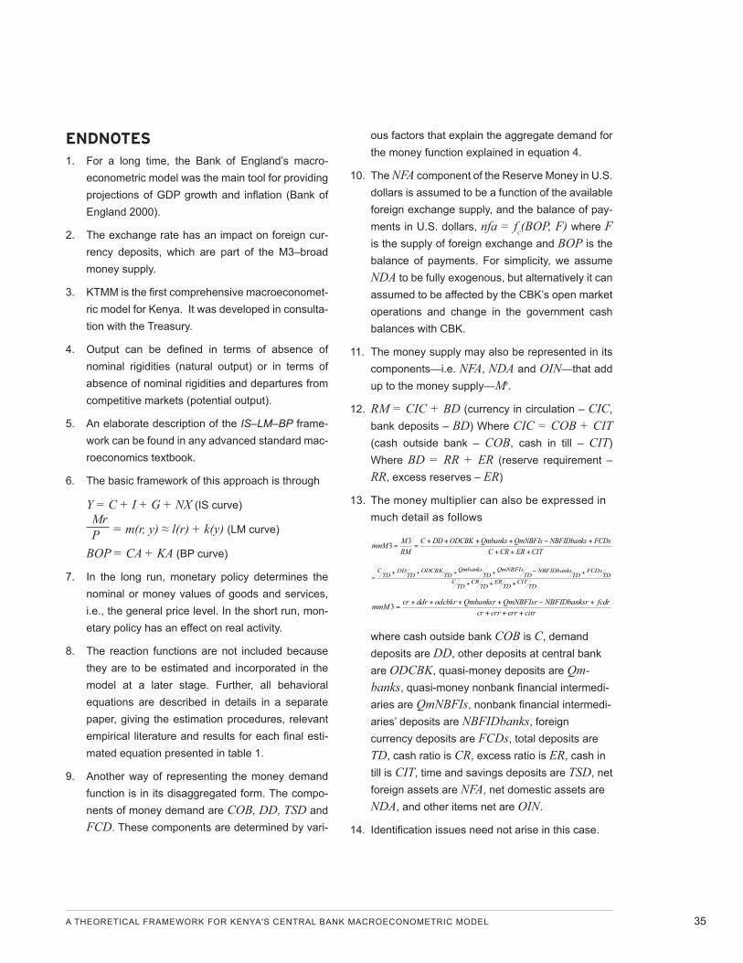
A THEORETICAL FRAMEWORK FOR KENYA'S CENTRAL BANK MACROECONOMETRIC MODEL 35
ENDNOTES1. For a long time, the Bank of England’s macro-
econometric model was the main tool for providing projections of GDP growth and inflation (Bank of England 2000).
2. The exchange rate has an impact on foreign cur-rency deposits, which are part of the M3–broad money supply.
3. KTMM is the first comprehensive macroeconomet-ric model for Kenya. It was developed in consulta-tion with the Treasury.
4. Output can be defined in terms of absence of nominal rigidities (natural output) or in terms of absence of nominal rigidities and departures from competitive markets (potential output).
5. An elaborate description of the IS–LM–BP frame-work can be found in any advanced standard mac-roeconomics textbook.
6. The basic framework of this approach is through
Y = C + I + G + NX (IS curve) MrP = m(r, y) ≈ l(r) + k(y) (LM curve)
BOP = CA + KA (BP curve)
7. In the long run, monetary policy determines the nominal or money values of goods and services, i.e., the general price level. In the short run, mon-etary policy has an effect on real activity.
8. The reaction functions are not included because they are to be estimated and incorporated in the model at a later stage. Further, all behavioral equations are described in details in a separate paper, giving the estimation procedures, relevant empirical literature and results for each final esti-mated equation presented in table 1.
9. Another way of representing the money demand function is in its disaggregated form. The compo-nents of money demand are COB, DD, TSD and FCD. These components are determined by vari-
ous factors that explain the aggregate demand for the money function explained in equation 4.
10. The NFA component of the Reserve Money in U.S. dollars is assumed to be a function of the available foreign exchange supply, and the balance of pay-ments in U.S. dollars, nfa = fc(BOP, F) where F is the supply of foreign exchange and BOP is the balance of payments. For simplicity, we assume NDA to be fully exogenous, but alternatively it can assumed to be affected by the CBK’s open market operations and change in the government cash balances with CBK.
11. The money supply may also be represented in its components—i.e. NFA, NDA and OIN—that add up to the money supply—Ms.
12. RM = CIC + BD (currency in circulation – CIC, bank deposits – BD) Where CIC = COB + CIT (cash outside bank – COB, cash in till – CIT) Where BD = RR + ER (reserve requirement – RR, excess reserves – ER)
13. The money multiplier can also be expressed in much detail as follows
CITERCRCFCDsNBFIDbanksQmNBFIsQmbanksODCBKDDC
RMMmmM
33
TDCIT
TDER
TDCR
TDC
TDFCDs
TDNBFIDbanks
TDQmNBFIs
TDQmbanks
TDODCBK
TDDD
TDC
citrerrcrrcrfcdrrNBFIDbanksQmNBFIsrQmbanksrodcbkrddrcrmmM
3
where cash outside bank COB is C, demand deposits are DD, other deposits at central bank are ODCBK, quasi-money deposits are Qm-banks, quasi-money nonbank financial intermedi-aries are QmNBFIs, nonbank financial intermedi-aries’ deposits are NBFIDbanks, foreign currency deposits are FCDs, total deposits are TD, cash ratio is CR, excess ratio is ER, cash in till is CIT, time and savings deposits are TSD, net foreign assets are NFA, net domestic assets are NDA, and other items net are OIN.
14. Identification issues need not arise in this case.

The views expressed in this working paper do not necessarily reflect the official position of Brookings, its board or the advisory council members.
© 2013 The Brookings Institution
ISSN: 2166-5184 (online) | 2166-5176 (print)
Cover photos courtesy of (left to right): Trevor Samson / World Bank, Hansjoerg Richter, John Hogg / World Bank, Andrew Martin Green, Lorenzo Codacci, Eric Miller / World Bank, Ami Vitale / World Bank

1775 Massachusetts Avenue, NW Washington, DC 20036 202-797-6000 www.brookings.edu/global