A Test setup for characterizing high-temperature

Rochester Institute of TechnologyRIT Scholar Works

Theses Thesis/Dissertation Collections

7-1-2013

A Test setup for characterizing high-temperaturethermoelectric modulesSatchit Mahajan

Follow this and additional works at: http://scholarworks.rit.edu/theses

This Thesis is brought to you for free and open access by the Thesis/Dissertation Collections at RIT Scholar Works. It has been accepted for inclusionin Theses by an authorized administrator of RIT Scholar Works. For more information, please contact [email protected].

Recommended CitationMahajan, Satchit, "A Test setup for characterizing high-temperature thermoelectric modules" (2013). Thesis. Rochester Institute ofTechnology. Accessed from

http://scholarworks.rit.edu?utm_source=scholarworks.rit.edu%2Ftheses%2F1297&utm_medium=PDF&utm_campaign=PDFCoverPages

http://scholarworks.rit.edu/theses?utm_source=scholarworks.rit.edu%2Ftheses%2F1297&utm_medium=PDF&utm_campaign=PDFCoverPages

http://scholarworks.rit.edu/etd_collections?utm_source=scholarworks.rit.edu%2Ftheses%2F1297&utm_medium=PDF&utm_campaign=PDFCoverPages

http://scholarworks.rit.edu/theses?utm_source=scholarworks.rit.edu%2Ftheses%2F1297&utm_medium=PDF&utm_campaign=PDFCoverPages

http://scholarworks.rit.edu/theses/1297?utm_source=scholarworks.rit.edu%2Ftheses%2F1297&utm_medium=PDF&utm_campaign=PDFCoverPages

mailto:[email protected]

i

A Test Setup for Characterizing High-

Temperature Thermoelectric Modules

by

Satchit B. Mahajan

A Thesis Submitted in Partial Fulfillment of the Requirements for the Degree of

Master of Science in Mechanical Engineering

Approved by:

Dr. Robert J. Stevens

Department of Mechanical Engineering

Dr. Satish G. Kandlikar


Dr. Michael G. Schrlau


Dr. Wayne W. Walter


______________________________

(Thesis Advisor)

______________________________

(Committee Member)

______________________________

(Committee Member)

______________________________

(Department Representative)

Sustainable Energy Systems Lab


Kate Gleason College of Engineering

Rochester Institute of Technology

July 2013

i

Abstract

With the tremendous growth in demand for energy resources, there is a growing need to adopt

alternative energy technologies, including ones that tap renewable energy sources as well as use

non-renewable sources more efficiently. Thermoelectric energy generation is one such emerging

technology. Thermoelectrics can convert waste heat from various sources—significantly, many

industrial processes as well as vehicles—directly into electrical power. Thermoelectric devices

can generate power when a temperature difference is applied across them. Major barriers to

mainstream adoption of thermoelectric devices are their low efficiency and high cost. These are

mostly limited by the properties of the constituent materials of the device(s) and the operating

temperatures. In the past decade there have been significant advancements in thermoelectric

materials that can be used at higher temperatures. The properties of thermoelectric materials are

temperature dependent, and may also vary from bulk material to device level. Right now, devices

with higher working temperatures are not available. According to feedback from laboratories

working on high-temperature modules, the next stage in the development of thermoelectric

devices would go up to 650°C.

The main focus of this project is to design and develop a test stand to evaluate the properties of

all such high-temperature devices. One of the critical challenges in testing modules, especially at

high temperatures, is being able to accurately control and measure heat rates transferred across a

module. Many of the current characterization techniques are limited to solely measuring the

electrical response and ignoring the heat transfer. A new testing technique, “rapid steady state,”

was developed, which is able to accurately measure the three key characteristic properties—the

Seebeck coefficient, electrical resistance, and thermal conductance—of a thermoelectric module

ii

over temperature ranges from 50 to 650°C. To ensure isothermal surfaces and minimize heat rate

errors, a primary heater is encased in a guard heater. Rapid pulsed electronic loading allows for

rapid voltage-current scans while avoiding thermal drift. The thermal conductivity of a reference

material is used to validate the performance of the guard heater assembly and heat-monitoring

setup.

iii

Acknowledgements

First and foremost I offer my sincere gratitude to my adviser Dr. Stevens for his knowledge,

understanding and most importantly patience while guiding me. He had faith in me even at times

when I did not. This project would never have been completed had it not been for his help. I am

not sure how many graduate students are fortunate enough to be given the freedom that you gave

me. For everything you’ve done for me, Dr. Stevens I thank you. I could not have wished for a

better adviser, as a teacher and a person.

I would like to thank NYSP2I for the Research and Development grant which helped fund the

project. I would also like to thank the members of my thesis committee for all their input and

ideas while designing the project. I want to thank Dr. Kandlikar for providing me my first

exposure to experimental testing and Dr. Schrlau for his ideas and insights.

I would like to thank Jan Maneti and especially Rob Kraynik at the Mechanical Engineering

machine shop for their immense help in building the test stand. I would be lost without their

help. I am also thankful to Dr. Hensel and everyone at the ME office for their guidance and

support during my time here at RIT. A special thank you goes to Dhruvang and Reggie, my lab

members for all of their help in completing my project and Sheryl who helped me polish my

thesis.

Finally, I want to thank my family, for always believing in me. They have always been a pillar of

unwavering support and gave me the strength to continue in the face of hardships. I hope that one

day I become at least half the person you thought I would be. I want to also thank my friends

Aditya and Zeeshan, my days in Rochester would be colorless without you. And last I want to

thank my girlfriend Devyani, for being my closest friend, confidant and my silver lining. I cannot

imagine being where I am now without your support.

iv

Table of Contents

CHAPTER 1. INTRODUCTION TO THERMOELECTRICS .............................. 1

1.1 Introduction .......................................................................................................................... 1

1.2 Advantages ........................................................................................................................... 2

1.3 Disadvantages ...................................................................................................................... 3

1.4 Applications ......................................................................................................................... 4

1.5 Background and Theory ....................................................................................................... 5

1.6 Significant Parameters ....................................................................................................... 10

1.7 Thermoelectric Materials ................................................................................................... 11

1.8 TEM Construction and Configuration ............................................................................... 13

CHAPTER 2. TESTING APPROACHES ............................................................17

2.1 Harman Approach .............................................................................................................. 17

2.2 Steady-State Approach....................................................................................................... 20

2.3 Other Testing Approaches ................................................................................................. 24

CHAPTER 3. PRELIMINARY TESTING ...........................................................28

3.1 Steady-State Method .......................................................................................................... 29

3.2 Harman Method ................................................................................................................. 33

3.3 Gao Min Method ................................................................................................................ 48

3.4 Conclusion ......................................................................................................................... 56

CHAPTER 4. DESIGN OF THE TEST APPARATUS .......................................58

4.1 Specifications ..................................................................................................................... 58

v

4.2 Build Overview .................................................................................................................. 60

4.3 Thermal Modeling ............................................................................................................. 63

4.4 COMSOL and ANSYS Models ......................................................................................... 77

4.5 Build Description ............................................................................................................... 84

4.6 Troubleshooting ................................................................................................................. 93

4.7 Rapid Steady-State Test ..................................................................................................... 98

CHAPTER 5. VALIDATION AND UNCERTAINTY ......................................108

5.1 Comparison With the Old Setup ...................................................................................... 108

5.2 Repeatability Testing ....................................................................................................... 109

5.3 Validation Using Reference Materials ............................................................................. 111

5.4 Uncertainty Analysis ........................................................................................................ 115

CHAPTER 6. CONCLUSION ............................................................................128

6.1 Summary of Results ......................................................................................................... 128

6.2 Contributions to the Thermoelectric Field ....................................................................... 130

6.3 Suggested Improvements and Future work...................................................................... 131

CHAPTER 7. REFERENCES .............................................................................134

APPENDIX A ......................................................................................................140

APPENDIX B ......................................................................................................141

vi

List of Figures

Figure 1.1: Seebeck Effect .............................................................................................................. 7

Figure 1.2: Peltier Effect ................................................................................................................. 8

Figure 1.3: Variation of ZT with temperature for different materials [11] ................................... 11

Figure 1.4: Development of ZT since 1940 [13] .......................................................................... 12

Figure 1.5: Typical thermoelectric module in heat pumping configuration ................................. 13

Figure 1.6: A typical TEM in power generation configuration .................................................... 13

Figure 2.1: Schematic of the test setup used by Mitrani et al. [27] .............................................. 19

Figure 2.2: Schematic of the test setup developed by Vazquez et al. [30] ................................... 21

Figure 2.3: Experimental setup developed by Sandoz-Rosado and Stevens [34]......................... 23

Figure 2.4: Sectional view of the setup used by Ponnambalam et al. [22] ................................... 25

Figure 3.1: A simplified schematic of the steady-state approach ................................................. 29

Figure 3.2: Module scan for steady-state approach [49]............................................................... 31

Figure 3.3: “Heat sunk” test configuration schematic .................................................................. 34

Figure 3.4: Current pulse applied to a TEM and the transient voltage generated due to it [50] ... 35

Figure 3.5: Schematic of the experimental setup for the positive and negative tests showing the

flow of heat from and into the module.......................................................................................... 37

Figure 3.6: Thermal modeling when current is applied in thermal equilibrium [28] ................... 38

Figure 3.7: Block Diagram of the experimental setup for Harman method ................................. 43

Figure 3.8: The plots for voltage and current ............................................................................... 44

Figure 3.9: The difference of the temperature readings ................................................................ 45

Figure 3.10: Thermal resistances in a TEM .................................................................................. 46

Figure 3.11: Schematic of the Gao Min approach ........................................................................ 49

Figure 3.12: The equivalent circuit for calculating the resistance ................................................ 53

vii

Figure 3.13: Schematic for the Gao Min approach ....................................................................... 55

Figure 4.1: Schematic of the entire setup...................................................................................... 62

Figure 4.2 Schematic of a thermoelectric leg pair ........................................................................ 65

Figure 4.3: Thermal circuit of the module .................................................................................... 66

Figure 4.4: Guard heater schematic showing the various zones. Also shown is the discretization

method of the guard heater ........................................................................................................... 72

Figure 4.5: Thermal circuit for calculating insulation losses ........................................................ 73

Figure 4.6: Cold side heater assembly .......................................................................................... 76

Figure 4.7: COMSOL simulation temperature distribution .......................................................... 82

Figure 4.8: Temperature distribution across the main heater ....................................................... 83

Figure 4.9: Temperature distribution across guard heater ............................................................ 84

Figure 4.10: Main heater assembly ............................................................................................... 85

Figure 4.11: Sensing thermocouple placement in setup ............................................................... 86

Figure 4.12: Control thermocouple placement in setup ................................................................ 87

Figure 4.13: Schematic of the argon purging system ................................................................... 90

Figure 4.14: Inert gas purging enclosure ...................................................................................... 92

Figure 4.15: Guard heater arrangement with finned base ............................................................. 93

Figure 4.16: New design for the guard heater............................................................................... 94

Figure 4.17: Thermal analysis on redesigned guard heater .......................................................... 95

Figure 4.18: Thermocouple calibration setup ............................................................................... 97

Figure 4.19: Temperature dependence of voltage with an increase in time step ........................ 100

Figure 4.20: Voltage response for applied current at 10ms time step ........................................ 101

Figure 4.21: Current-voltage scan and linear curve fit for a 100°C temperature difference, with

the hot side and cold side temperatures being 170˚C and 70˚C, across a typical BiTe module . 102

Figure 4.22: Screenshot of the LABVIEW program .................................................................. 105

viii

Figure 5.1: Comparison of the characteristic module properties measured by the rapid steady-

state approach and the regular steady state approach [34] .......................................................... 109

Figure 5.2: Comparison of power output vs. load voltage for different temperature differences

..................................................................................................................................................... 110

Figure 5.3: Comparison of voltages and current measurements for different temperature

differences ................................................................................................................................... 111

Figure 5.4: Comparison of measured conductivity of borofloat and reference values ............... 113

Figure 5.5: Comparison of measured conductivity of quartz glass and reference values ........... 114

ix

List of Tables

Table 2.1: Summary of Literature ................................................................................................. 26

Table 3.1: Steady-State Results for = 150°C and = 50°C................................................... 32

Table 3.2: Comparison of Thermoelectric Module Properties Measured By the Steady-State

Approach and Modified Harman approach................................................................................... 45

Table 3.3: Thermal resistances for a module ................................................................................ 47

Table 3.4: Comparison With Steady-State Results After Correction ........................................... 48

Table 3.5: Comparison of Gao Min results with Steady state ones, showing the effect of well

calibrated resistors ........................................................................................................................ 56

Table 4.1: The Material Properties Used in Simulation of Extreme CasesTable ......................... 70

Table 4.2: Properties of Four Extreme Sizes of Thermoelectric Modules ................................... 70

Table 4.3: Heat Losses Calculated (to the Main Heater and to Surroundings) ............................. 74

Table 4.4: Cold Plate Heat Flux for Different Temperature Differences ..................................... 77

Table 4.5: Material Options for Heaters ....................................................................................... 79

x

Nomenclature

Symbol Parameter

Surface Area, m2

Current flowing through the leg pair or module, A

Thermal conductance, W/K

* Coverage Factor

Power generated by a leg pair or module, W

Heat rate, W

Electrical resistance of a module, Ω

Thermal Resistance, K/W

Temperature, K or °C

Uncertainty in a measured quantity, %

Voltage across a leg pair or module, V/K

Figure of merit, dimensionless

xi

Symbol Parameter

Seebeck coefficient, V

Thompson coefficient, W/mAK

Temperature difference across the module, °C

Module efficiency, %

Thermal conductivity, W/mK

Peltier coefficient, W/A

Electrical resistivity, Ωm

Standard deviation in measurement, takes dimension of measured quantity

xii

Subscript Parameter

Averaged result for tests carried out using positive and negative current

Property measured during negative current test

Property of aluminium block

Cold side, K or °C

Cold plate properties

Hot side, K or °C

Property evaluated after applying electrical loading

Open circuit

Short circuit

Thermoelectric module

Property measured at ambient condition

Properties of thermal bypass

Properties of ceramic plate

Equivalent

Property along insulation

Properties of the interconnect material

Module property

Property of a n-leg

Seebeck component

Property of a p-leg

Overall property over p-leg and n-leg

Resistive component

Component of Random uncertainty

Component of Systematic uncertainty

Properties of Shunt resistor

Uncertainty component of temperature

xiii

Uncertainty component of voltage

Module conduction losses

Page | 1

Chapter 1. Introduction to

Thermoelectrics

1.1 Introduction

In the year 2008, total world requirement for energy was 500 quadrillion BTU [1], approximately

50% of which was dumped into the environment in the form of waste heat. Waste heat is heat

generated in a process by way of fuel combustion or chemical reaction, then “dumped” into the

environment even though it could still be reused for some useful and economic purpose. In the

industrial sector 20–50% of the energy input is lost as waste heat [2].

The energy lost in waste heat cannot be fully recovered because it is often low-grade heat and

dispersed. With the world’s population growing at the rate of 1.1% per year, the energy

requirement is expected to double by 2020 [3]. Coupled with this is the rapid depletion of fossil

fuel global reserves. There is a widespread need for alternative sources of energy and energy

conversion technologies.

The use of thermoelectrics is potentially one such opportunity. Thermoelectric modules (TEMs)

can generate power when placed between a heat source and a heat sink. TEMs are increasingly

finding application in waste heat regeneration such as automobiles, industrial processes, and

power plants. This is a process wherein heat energy that would have been dissipated into the

atmosphere is utilized for generating power. Thermoelectrics are also environmentally friendly

and generate no emissions.

Page | 2

Another important application of thermoelectrics is as Peltier coolers. These are extensively used

in electronic devices that have specified cooling requirements. Precise temperature control and

the abbility to cool below atmospheric temperatures make them an ideal candidate in computer

electronics.

1.2 Advantages

There are many advantages to using thermoelectrics. These are summarized as follows:

No moving parts: Thermoelectrics can generate electricity directly without any moving parts so

they are virtually maintenance free. In fact, one of the first applications of thermoelectrics was

and still is to power deep space probes using radioisotopes as heat sources. These systems have

functioned for decades with no maintenance [4].

Small size and weight: The overall thermoelectric cooling system is much smaller and lighter

than a comparable mechanical system. In addition, a variety of standard and special sizes and

configurations is available to meet strict application requirements. Thermoelectrics are modular

and can be used for a range of applications. Current systems operate over a wide range, from

mW to KW.

High reliability: Thermoelectrics exhibit very high reliability due to their solid state

construction. Although reliability is somewhat application dependent, the life of typical

thermoelectric coolers is rated to be greater than 200,000 hours. The actual life of the modules

may be much longer. In fact, the modules used by NASA in their long-range satellites are still

functioning with no maintenance even after several decades in operation.

Page | 3

Operational conditions: Thermoelectrics can be used in any orientation and adverse

environments, as well as over a large range of temperatures. This makes them ideal for

applications based on waste heat utilization.

Transient heat sources: TEMs can be used in applications where the heat source is not constant.

This is a huge benefit in applications like waste heat utilization of automobile exhaust, where the

heat source is variable and where other power recovery technologies are not feasible.

1.3 Disadvantages

Though thermoelectrics have many advantages, there are drawbacks in the technology. These are

summarized as:

Low efficiency: This is a major drawback facing the thermoelectric industry. Current off-the-

shelf thermoelectric devices efficiencies are typically in the range of 2–8%. Thermoelectrics

have been mainly confined to low-energy applications or where the heat source is free, and are

unable to compete for large-scale power generation applications.

Susceptibility to shock loading: Thermoelectrics can handle transient heat loads, but the life of

thermoelectric devices decreases considerably after receiving thermal shock loading. In the case

of mechanical loading, they can withstand up to 1000 psi but only to the standard loading—

around 200psi—in compression. They are weakest in shear loading [5].

Cost: Owing to the novelty of the technology, the cost per watt of the device is much higher than

with the conventional power generation technologies. As newer and cheaper materials with

higher power ratings are developed and manufacturing techniques are improved, the cost per unit

power is certain to decrease.

Page | 4

1.4 Applications

Peltier cooling

Peltier cooler is a thermoelectric operating in heat pumping mode. As current is passed through a

thermoelectric device, a temperature difference develops across it. The cold side of the device is

thermally coupled with the component being cooled, while the hot side of the device needs to be

cooled externally using a heat sink or forced convection. Peltier coolers have an important role in

electronics, especially in cases where conventional cooling systems cannot be implemented.

Their small size, silent operation, and the ability to maintain the temperature accurately make

them especially attractive for use as CPU coolers [6].

Thermoelectrics are also used in microelectronics where localized cooling is required. Gupta et

al. [7] investigated the operation of a ultrathin thermoelectric cooler for cooling of localized hot

spots on a chip. They found the device to be very effective for low-current operations. However,

as the current increased over 4A, back heat flow due to the temperature difference generated

countered the cooling effect.

Other niche applications include refrigeration, in wine coolers, car refrigerators, and beverage

can coolers. Thermoelectrics are also used in NEMA enclosures to regulate temperatures and

applications where cryogenic cooling is required.

Power generation

While thermoelectrics are not currently used in a wide range of power generation applications,

their most important application will undoubtedly be in power generation. An important factor is

that TEMs can utilize waste heat from a large number of processes for power generation. The

Page | 5

energy conversion efficiency is low compared to other power conversion technologies, which is

the main hurdle to be crossed before thermoelectric moves from a niche to mainstream power

generation applications.

Low-power applications include powering watches, calculators, and remote sensing. The

“Thermic” [8] designed by Seiko used body heat for its working. Thin film micro generators

producing power at milliwatt and microwatt level are used in electronic applications. Kim [9]

fabricated one such device generating 4.3nW/K. These can be coupled easily with photovoltaic

cells as well.

Thermoelectrics have found application in high-power generation as well, but the major

drawback is the low efficiency. They are mainly used in waste heat applications, where the

supply of heat is free. Commercially, modules generating up to 550W are available. Standalone

thermoelectric generators are mainly used in extreme environments.

Thermoelectrics have been critical in enabling continuous powering of deep space probes where

the use of solar and other power generation technologies is not feasible. For example,

thermoelectrics are used in radioisotope thermoelectric generator (RTG) where power is

generated using heat from the decay of radioactive material, like plutonium-238. Over the last

four decades, 26 missions have used RTGs. The RTG installed on the Mars rover is expected to

operate for at least one Mars year or 687 Earth-days.

1.5 Background and Theory

Thermoelectric devices are basically solid state devices that can convert energy from heat to

electricity or vice versa. Devices are normally made up of semiconductor materials, the most

Page | 6

common being bismuth telluride. A typical configuration of a thermoelectric module consists of

many leg pairs made of semiconductor pellets, joined together using contact tabs made of high

conductivity materials.

Seebeck Effect

The principle behind the working of the thermoelectric module is the Seebeck effect. In 1821

Thomas Johann Seebeck observed that when two dissimilar metals with junctions at different

temperatures are connected in a circuit, a magnetic needle would be deflected. Seebeck initially

attributed this phenomenon to magnetism. However, it was quickly realized that it was an

induced electrical current that deflects the magnet [10]. In a thermoelectric module, the two

dissimilar conductors are connected electrically in series and thermally in parallel. When the two

junctions are maintained at temperatures and respectively, and > , an open circuit

electromotive force ( ) is developed between the junctions, as seen in Fig. 1.1.

Page | 7

Heat In

Heat Out

Hot Junction (TH)

Current

Power Generation

Cold Junction (TC)

Figure 1.1: Seebeck Effect

The voltage produced is proportional to the temperature difference between the two junctions.

This is given by:

(1.1)

The proportionality constant, α, is the difference between the Seebeck coefficients of the two

materials forming the junction. This is known as the overall Seebeck coefficient, and often

referred to as the thermoelectric power or thermo power. The Seebeck voltage does not depend

on the distribution of temperatures along the material between the junctions. This phenomenon is

what is used to measure temperatures using thermocouples.

Page | 8

Peltier Effect

The converse of the Seebeck effect was discovered independently by Jean-Charles Peltier in

1834. When current is made to flow through a junction of dissimilar materials, a rate of heating

occurs at one junction while heat is absorbed at the other junction [10]. Although it is the

converse of the Seebeck effect, Peltier failed to make the connection when he discovered the

phenomenon. In Fig. 1.2 it can be seen that when a current is passed through the junction, one

side is heated and the other is cooled.

Figure 1.2: Peltier Effect

The Peltier co-efficient is defined as:

(1.2)

Page | 9

where Q is the rate of heating or cooling and I is current passing through the junction. The Peltier

coefficients represent how much heat current is carried per unit charge through a given material

[10].

Thomson effect

The Thomson effect was observed by Sir William Thomson in 1851. It relates to the rate of

heating or cooling resulting from the passage of current through a current-carrying conductor

with a temperature gradient applied across it, and is defined as the evolution or absorption of

heat when electric current passes through a circuit composed of a single material that has a

temperature difference along its length. If ( ) is the temperature difference generated across a

conductor carrying current ( ), then heat generated per unit length ( ) is given by

(1.3)

where is the Thomson coefficient.

The Kelvin Relationships

Lord Kelvin developed relationships between the above three thermoelectric coefficients. The

relationships were tested for many thermoelectric materials and it is assumed that they hold true

for all materials used in thermoelectric applications.

The relationships can be written as:

(1.4)

(1.5)

where T is the absolute temperature.

Page | 10

1.6 Significant Parameters

The most important parameters in a thermoelectric material are the “Seebeck coefficient” and

“figure of merit.” The Seebeck coefficient is a measure of the transported entropy per charge

carrier. The figure of merit is a non-dimensional measure of performance of the material. It gives

the theoretically possible maximum efficiency of a thermoelectric.

The figure of merit (ZT) is expressed as

(1.6)

The figure of merit varies directly with the Seebeck coefficient and electrical conductivity and

inversely with thermal conductivity. An increase in electrical conductivity reduces the losses

caused due to Joule heating. A decrease in the thermal conductivity would limit the amount of

heat passing through the module without being converted into power. The theoretical maximum

efficiency of thermoelectric material depends on the figure of merit, and there are no theoretical

upper limits for the figure of merit. Most materials currently used have thermoelectrics of

approximately one or less. Figure 1.3 shows the relationship between the TZ values of different

materials and temperature.

Page | 11

Figure 1.3: Variation of ZT with temperature for different materials [11]

Though the ZT value is the measure of a Carnot performance, it does not exactly translate to the

module efficiency. The efficiency actually is based on the amount of heat flowing through the

module itself, not the amount of heat available. A clear trend is observed, where ZT for a given

material increases as its temperature increases. Currently, the best thermoelectric materials

developed in the lab have values between one and three[11], but these are yet to be used in

practical devices.

1.7 Thermoelectric Materials

Low efficiency of the thermoelectric modules is a significant drawback hindering the use of

thermoelectric modules in everyday applications. As seen in the previous section, a higher ZT

Page | 12

begets better efficiency. Hence, extensive research is being carried out to find a material with

high ZT and to improve the ZT values of existing materials.

In the literature today, the best materials currently used in most thermoelectric devices have ZT

values between zero and three. Some of the most popular materials have been bismuth telluride

(Bi2 Te3 system) and silicon-germanium combinations. Much research has been carried out on

these materials and the scope of improvement is small. Consequently, newer and better materials

are being investigated, primarily by nano-engineering materials. Figure 1.4 below shows a plot

of ZT as a function of temperature for the various nanostructured bulk materials being developed

in labs. There have been tremendous improvements in thermoelectric materials, primarily driven

by improved understanding of thermal transport at the nanoscale and improved nanostructure

fabrication techniques [12].

Figure 1.4: Development of ZT since 1940 [13]

Page | 13

1.8 TEM Construction and Configuration

A typical thermoelectric module is made of multiple leg pairs, where each leg pair is made of

two semiconductor materials made from p and n type semiconductor materials. The combination

of these multiple leg pairs is held together by a top and bottom plate, typically made of a

ceramic-like aluminum nitride (AIN). This ensures electrical insulation and structural support.

The leg pairs are connected in such a way that they are in series electrically and in parallel

thermally. The pellets, tabs, and ceramic plates form a layered configuration, as seen in Fig 1.5.

Figure 1.5: Typical thermoelectric module in heat pumping configuration

Generally the individual legs are made of a single material. But as newer technologies are

developed, leg pairs made up of multiple materials are being developed.

Figure 1.6: A typical TEM in power generation configuration

Page | 14

Figure 1.6 shows a module in a power generation arrangement where heat enters the hot side of

the module and is rejected from the cold side of the module. The most commonly used approach

for calculating power generation is a one-dimensional approach. Using the model developed by

Angrist [14] , the heat flow into the hot side of the module, , is expressed as

⁄ (1.7)

where I is the current flowing through the module and is the overall Seebeck coefficient,

which is the product of the difference of the individual Seebeck coefficients of the two

constituent materials and the number of leg pairs. and are the temperatures on the hot and

cold sides of the module. K is the thermal conductance, which is the inverse of the thermal

resistance across the entire device. This includes the thermal resistance of the legs as well as the

thermal resistance of the substrate and thermal leakage across the device. R is the electrical

resistance, which includes the leg and metal connector contact resistance. The heat flow out of

the module ( ) is given by

⁄ (1.8)

These expressions are developed by solving the heat diffusion equation in the device and

applying a fixed temperature and the Peltier effect model at the surfaces. From energy

conservation, the electrical power output of a thermoelectric module is expressed as

(1.9)

(1.10)

Page | 15

The efficiency of the module can be expressed as the ratio of the power output to the heat input,

and is given as

(1.11)

⁄ (1.12)

Most of the modules commercially available today can be classified as “low temperature.”

Research conducted on low-temperature waste heat recovery systems [15–19] has demonstrated

the potential viability of thermoelectric systems. However, the primary reasons that

thermoelectrics have not been adopted in mainstream applications are low efficiency and high

cost. The efficiency of the module generally increases as the temperature difference applied

across it increases. To achieve improved efficiency, there is interest in developing high-

temperature materials to enable operation of modules at higher temperature differences than

those reached with typical BiTe-based devices.

In conclusion, over the past decade there have been significant advancements in thermoelectric

materials that can be used at high temperatures [20–24]. More recently, TEMs based on these

materials have also been developed. Thus, developing the capability to test high-temperature

thermoelectric devices is desperately needed to support the development of ceramic oxide-based

thermoelectrics. Such capabilities do not currently exist. The testing system proposed in this

thesis will provide the ability to demonstrate proof of concept of the next generation of

thermoelectric devices using oxides and other high-temperature materials, provide experimental

data to validate and improve device models, and characterize devices for system design

Page | 16

purposes. The testing capabilities will also allow for an efficient means of optimizing devices

and a better understanding of the impact of various material interface and fabrication options.

Page | 17

Chapter 2. Testing Approaches

In the field of thermoelectrics, there are two categories of testing. The first is testing of materials,

and the second is testing of modules or devices. A wealth of research on the testing and

characterization of thermoelectric materials exists. However, little has been done to test complete

power generation modules. Material testing cannot account for different performance effects

such as diffusion losses, contact resistance, thermal strain, and thermal cycling that occur in

power generation modules. Module level testing is also vital for quantifying device performance,

validating existing models, and optimizing module design, as well as testing for longevity and

reliability of a device.

There have been two main approaches used for characterizing modules in the literature: the

Harman approach and the steady-state approach. Both approaches have been utilized for low-

and high-temperature testing in literature. This chapter describes some of the setups and analysis

used for testing modules as well as bulk materials.

2.1 Harman Approach

The Harman approach [25] was initially developed for bulk material testing, but has been

adopted and used for module testing. The technique is based on the Peltier effect of a

thermoelectric material, specifically the heating and cooling at the module interfaces when a

current is applied. When a current is passed through a module, the voltage across the module

rises instantaneously to the electrical resistance component of the module, and then

Page | 18

asymptotically increases to the steady-state voltage, which is the sum of the resistive and

Seebeck voltage. The Seebeck voltage is caused by the temperature difference developed in the

device due to the Peltier cooling. The voltage is given by Eq. (1.1). When the current is removed

from the module, the voltage drops instantaneously to the Seebeck component of the voltage and

then decays to zero as heat conducts across the module and returns to being isothermal. The

various properties are calculated using these voltages and resulting temperatures, and is

described in detail in Section (3.2).

The method initially developed by Harman [25] uses the difference between the total voltage and

the electrical resistance component of the voltage to calculate the Seebeck coefficient for the

module. The method does not take into account effects like Thomson heating and joule heating,

and heat losses due to conduction are assumed to be negligible. The method was validated by

comparing values of properties with a reference material. A variation of this method was

developed by Buist [26]. It uses the Seebeck component of voltage measured; specifically, the

voltage immediately after the applied current is removed, to calculate the Seebeck coefficient.

The approach called for bipolar testing to reduce errors and maximize accuracy of the results.

This is explained in detail in Section (4.2). The method also includes a correction factor for the

various heat losses.

Mitrani et al. [27] successfully used Buist’s method to calculate module performance parameters.

Instead of performing an energy balance, they used a reference material (aluminum) to calculate

the thermal conductance of the module. The results were found to match the ones from steady-

state testing as well as from electrothermal modeling in SPICE. A drawback of this general set of

approaches is that it is difficult to measure thermoelectric properties above room temperature.

This is because heat losses to the environment increase as the temperature increases above that of

Page | 19

the ambient, which makes it difficult to maintain adiabatic conditions on the module. Figure 2.1

shows the schematic of the test setup used.

Figure 2.1: Schematic of the test setup used by Mitrani et al. [27]

Fujimoto et al. [28] attempted to overcome the issues with high-temperature testing by reducing

thermal heat flow from the environment with a thermal anchor and a thermal reflector. They also

accounted for heat losses from wire conduction and ambient radiation. An important discovery

made while testing was that the largest cause of contact resistance was improper soldering at

contacts. They applied corrections to better account for the effect of contact resistance, and

reduced it by using a particular soldering technique.

The Harman approach can overlook convection losses by using a low vacuum. In cases where a

vacuum is not used, a correction factor was developed by Lau [29] to account for convection

effects. The correction factor was obtained by testing a module in both air and a vacuum and

comparing the results. However, even with the correction factor, it was observed that some

effects cannot be completely accounted for. Although this approach is extensively used with

Page | 20

materials with good, repeatable results, most of the testing is performed at room temperature.

Consequently, one of the downsides is that modules are not tested under typical operating

conditions.

2.2 Steady-State Approach

The second approach, the steady-state approach, ensures modules are tested under more realistic

operating conditions. The testing approach is for a steady setup is relatively straightforward and

the most common approach for module testing. One of the surfaces of the module is maintained

at a high temperature while the other is maintained at a lower temperature. According to the laws

of thermoelectricity, specifically the Seebeck effect, a potential difference is developed across

the module. By measuring the heat flows into or out of the module along with the voltage and

current, the module parameters can be estimated. An important assumption for the steady-state

approach is that all heat losses are measurable and accounted for. Measuring the exact amount of

heat rate flowing into or from the module is of utmost importance. However, obtaining an

accurate measurement is often challenging. As this is such an important part of the approach, the

various test stands in literature have been classified based on how they account for heat losses.

They are classified as basic setups, where the heat losses are considered negligible because the

setup is insulated well; passive accounting, where the heat losses are accurately measured and

accounted for; and active accounting, where the heat losses are measured as well as minimized

by using special guards.

Basic setups

Vazquez et al. [30] describe one such test stand for temperatures up to 300°C. The temperature

limit was a result of the heater material selected, Duralumin. Two types of tests were performed;

Page | 21

one varied the hot side temperature and the second varied the hot side heat flux. The cold side

was kept at a constant temperature. The various properties were calculated by loading the

module with various resistors and plotting the relationship of the voltage versus the current. One

drawback of the setup is that it does not account for any heat losses. The schematic of the setup

is shown in Fig. 2.2.

Figure 2.2: Schematic of the test setup developed by Vazquez et al. [30]

Tanji et al. [31] developed a steady-state test setup for testing of modules developed by a new

type of assembly method. The setup observes the importance of applied pressure on the module

and the effect of contact resistance. To reduce the contact resistance, they used a metallic paste

of liquid InGa and solid Zn.

Another setup was developed by Hsu et al. [32] for modules up to 250°C. Although they did not

account for heat losses, they provided a good explanation for the difference between material and

module properties. They also observed the effect of loading pressure on the measured module

parameters. Furthermore, an important method of relating the measured and theoretical

properties was developed. The properties discussed in the previous literature were material

properties, and the authors found large discrepancies when they were compared with their

Page | 22

experimental results. The main reason for the discrepancy was the effect of the temperature

gradient across the components of the module. This gradient was accounted for by using thermal

resistances across each component to determine the actual temperature gradient across the

thermoelectric module.

Passive accounting

Anatychuk and Havrylyuk [33] developed a test stand for measuring parameters up to 600°C that

accounts for heat losses from the hot side to the surrounding environment. The test stand uses a

heat meter attached to the cold side heat exchanger, which measures the heat flux flowing out of

the module. The heat meter used was a reference material of known conductivity such that the

exact heat rate could be calculated using the temperature difference measurement. At steady-

state conditions, it was assumed that the amount of heat flowing in will be equal to the amount of

heat flowing out of the module. In order to accommodate different-sized modules, the setup

employed interchangeable heat meters with an area resembling the module being tested. To

minimize errors, the hot side was well calibrated using a protective heater. The authors also

calculated the uncertainty in measurement, which was found to be 3%.

Another test stand was created by Sandoz-Rosado and Stevens [34] to characterize modules up to

500°C. The heat losses through the insulation on the top and sides of the heater as well as

through the insulation surrounding the sides of the module were measured. A power analyzer

measured the power input to the heaters. The authors also accounted for the effect of contact

resistance by loading the module with different pressures to measure its performance. Figure 2.3

shows a schematic of the setup.

Page | 23

Figure 2.3: Experimental setup developed by Sandoz-Rosado and Stevens [34]

Muto et al. [35] developed a setup used to measure properties of bulk materials for temperatures

up to 200°C with low uncertainty. These measurements also included the effects of side wall

radiation and contact resistance. The researchers encountered large heat losses from the hot side

assembly. To overcome this issue, they used a well-calibrated flux sensor on the cold side to

measure the heat flux, which accounted for heat losses by calibrating the flux sensors. The

authors used both approaches of the passive accounting—calculating heat losses and using a heat

meter—to verify their calculations.

Although these techniques are used extensively at lower temperatures, calculating heat losses at

higher temperatures leads to large uncertainties in measurements. The use of a reference material

also has certain drawbacks, the most important being the accuracy of data available for the

reference materials, which has an uncertainty of at least 5%. Other problems include difficulty in

Page | 24

measuring accurate temperature gradients within the reference material as well as calculating

heat losses from the reference material.

Active accounting

To overcome the inherent errors in using passive accounting techniques, researchers have used

radiation shields and shielding heaters to minimize heat losses. Rauscher et al. [36,37] use a

shielding heater to minimize heat losses. The principle behind this approach is that any heat loss

is related to a temperature difference in the system. If this difference is minimized, the losses can

be minimized. A shielding heater is basically an outer heater that surrounds the heater in contact

with the thermoelectric module. This ensures that all the heat supplied to the main heater block

passes through the module and not to the surroundings. A similar approach was used by

Takazawa et al. [38] in their setup to test modules up to 550K. They utilized a radiation shield to

reduce heat losses at the upper temperature limits.

2.3 Other Testing Approaches

Apart from the two main approaches described above, researchers have also experimented with

other methodologies to measure thermoelectric module parameters. Min and Rowe [39–41]

developed a testing method based on the steady state but eliminating the need to measure the

heat fluxes. This novel method utilizes an open-circuit and short circuit measurement to calculate

module parameters. Even though it is steady state, it does not require the measurement of the

exact amount of heat flowing through the module. This makes it especially attractive at high

temperatures, where this measurement is difficult by traditional means. To investigate its

application at high temperature, a detailed analysis was performed which is described in Section

(3.3).

Page | 25

Similar to the Harman method, a transient method was developed by Middleton and Scanlon

[42]. They used the method to measure the thermoelectric properties of germanium from 78–

925K. The Seebeck coefficient was calculated using the change in voltage brought about by the

change in temperature. To calculate the electrical resistance, the voltage response on the passage

of current was used. This approach is known as the differential approach and was developed

specifically for bulk materials. Sharath Chandra et al. [43] and Paul [44] developed high

accuracy setups based on this approach. The setup developed by Ponnambalam et al. [22] is

shown in Fig. 2.4.

Figure 2.4: Sectional view of the setup used by Ponnambalam et al. [22]

Table 2.1 shows a brief summary of the different testing methods reported in the literature along

with temperature ranges and device materials tested.

Page | 26

Table 2.1: Summary of Literature

Author Approach Temp. Range Material Vacuum

Harman, T. C.

[25]

Harman 300K Bismuth telluride Low vacuum

Buist and

Richard [26]

Harman <330K N-type bismuth

telluride

—

Mitrani et al.

[27]

Harman 300K Module —

Fujimoto et al.

[28]

Harman <600K N-type bismuth

telluride

Low vacuum

Lau [29] Harman 300K Module Low vacuum, air

Vazquez et al.

[30]

Steady state <573K Module —

Tanji et al. [31] Steady state <573K Module —

Hsu et al. [32] Steady state <523K

Module —

Anatychuk and

Havrylyuk [33]

Steady state <873K

Module —

Sandoz-Rosado

and Stevens [34]


Muto et al. [35] Steady state <473K P-type bismuth

telluride

Torr

Rauscher et al.

[36]

Steady state <573K Module Low vacuum

Rauscher et al.

[37]

Steady state <573K Module Torr

Takazawa et al.

[38]


Ahiska and

Ahiska [45]


Page | 27

Author Approach Temp. Range Material Vacuum

Ciylan and

Yilmaz [46]


Min and Rowe

[39–41]

Steady-state

based

<373K Module —

Iwasaki et al.

[47]

Harman based <315K Module Torr

Middleton and

Scanlon [42]

Differential 78–925K Germanium High vacuum

Paul [44] Differential 100–600K P-type PbTe 5 Torr

Sharath Chandra

et al. [43]

Differential 300K Al doped FeSi

platinum

Torr

From the literature review, it is clear that gaps exist in the area of high-temperature testing of

modules. The main reason for this is modules that can be tested at high temperatures have yet to

be developed. The high temperature setups developed are also found to yield fairly inconsistent

results because of a lack of standardized guidelines for the measurement procedure [22,48]. This

makes the selection of testing approach very difficult.

In summary, the popular choice for module testing seems to be the steady-state approach, but

high temperature testing will encumber active accounting of heat losses. The Harman approach,

though not extensively used for module testing at high temperatures, was the most used for

testing of material properties. The Gao Min approach is also a possible choice as it does not

require any measurements of the heat rates.

Page | 28

Chapter 3. Preliminary Testing

Preliminary testing is important gauging response time of the setup, determine ability to maintain

operating conditions and determine accuracy of instrumentation required. Of the various

approaches discussed in the literature for measuring module parameters, three were narrowed

down as candidates for the proposed high-temperature testing system. To determine the best

overall testing system, three preliminary setups based on the principles of the steady-state [34]

approach, Harman [26] approach, and the Gao Min [39] approach were developed to better

understand the various issues associated with each method before designing the high-temperature

test setup, the primary goal of this research.

The results from the three setups were compared for modules at low temperatures. Information

about module parameters is readily available for low temperatures, making comparison easy. A

commercially available BiTe module (Thermonamic Electronics TEP1-1264-1.5) with 126 leg

pairs was used. The size of the module was 40mm x 40mm, with 50% fill area, meaning 50% of

the module was air. Tests were conducted at a constant loading pressure and with thermal grease

on both sides of the module. Considering the rudimentary design, an uncertainty of 10% was

assumed. All the tests were performed at an average temperature of 100°C to keep the results

comparable. Multiple tests were performed on the same module to ensure repeatability in

measurements. All measurements were made using the same DAQ devices: NI–USB 6008 for

voltage and current readings and NI–TC 2095 for temperature readings.

Page | 29

3.1 Steady-State Method

The test setup developed by Sandoz-Rosado and Stevens [34] was successful as a tool for

characterization of module performance. The major achievement in the setup was to quantify the

heat transfer to the hot side of the module while adjusting the temperature difference across

devices under a wide range of electrical loads. Using measurements of the current, voltage, and

the hot side and cold side temperatures, the Seebeck level of the device, electrical resistance, and

thermal conductance parameters can be determined. Tests were carried out at various loading

pressures and temperatures, and a platform for characterizing module performance was

developed. Working with this test setup provided an insight into the various problems that may

arise, albeit only for low temperatures. A simplified schematic of the steady-state approach can

be seen in Fig. 3.1.

Figure 3.1: A simplified schematic of the steady-state approach

Page | 30

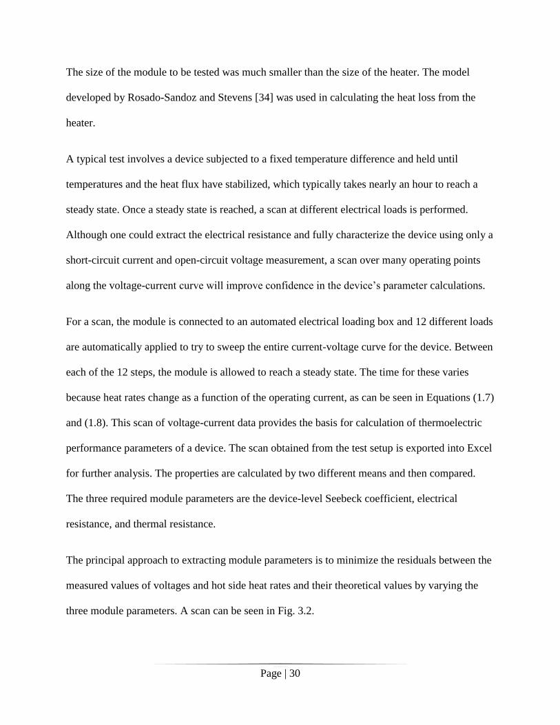
The size of the module to be tested was much smaller than the size of the heater. The model

developed by Rosado-Sandoz and Stevens [34] was used in calculating the heat loss from the

heater.

A typical test involves a device subjected to a fixed temperature difference and held until

temperatures and the heat flux have stabilized, which typically takes nearly an hour to reach a

steady state. Once a steady state is reached, a scan at different electrical loads is performed.

Although one could extract the electrical resistance and fully characterize the device using only a

short-circuit current and open-circuit voltage measurement, a scan over many operating points

along the voltage-current curve will improve confidence in the device’s parameter calculations.

For a scan, the module is connected to an automated electrical loading box and 12 different loads

are automatically applied to try to sweep the entire current-voltage curve for the device. Between

each of the 12 steps, the module is allowed to reach a steady state. The time for these varies

because heat rates change as a function of the operating current, as can be seen in Equations (1.7)

and (1.8). This scan of voltage-current data provides the basis for calculation of thermoelectric

performance parameters of a device. The scan obtained from the test setup is exported into Excel

for further analysis. The properties are calculated by two different means and then compared.

The three required module parameters are the device-level Seebeck coefficient, electrical

resistance, and thermal resistance.

The principal approach to extracting module parameters is to minimize the residuals between the

measured values of voltages and hot side heat rates and their theoretical values by varying the

three module parameters. A scan can be seen in Fig. 3.2.

Page | 31

Figure 3.2: Module scan for steady-state approach [49]

The theoretical heat rate is given by Eqn. (1.7) and the theoretical voltage can be obtained by

dividing the power Equation (1.10) by the current to give the voltage as:

(3.1)

Residuals are measured as the square of the difference between the two values to account for

positive and negative errors. The minimization provides one set of the values of the module’s

parameters, the slope, and the y-intercept of the current-voltage line.

The y intercept gives the open-circuit voltage ( ) and the slope of the plot is equivalent to the

electrical resistance ( ). The Seebeck coefficient ( ) is calculated as:

(3.2)

Page | 32

The thermal conductance of the module can be expressed as the ratio of the actual heat to the hot

side of the module under open-circuit conditions to the temperature difference across the

module:

(3.3)

The module effective figure of merit, ZT, is calculated as:

(3.4)

The values obtained from Eqns. (3.2) - (3.4), and the slope of the line ( ), are compared with the

values from the minimization scheme. The two sets of values are found to be in agreement with a

difference of less than 5%.

The tests were carried out multiple times to test for repeatability. The results, averaged over

multiple tests, were tabulated as seen in Table 3.1.

Table 3.1: Steady-State Results for = 150°C and = 50°C

Properties Steady State (397K)

α (V/K) 0.044

R (Ω) 2.42

K (W/K) 0.63

ZT 0.47

As mentioned earlier, as this setup is the most developed one, it will be used for low-temperature

benchmarking of the preliminary setups of the two other approaches.

Page | 33

3.2 Harman Method

To obtain accurate results, the steady-state approach requires careful estimation of all possible

heat losses, which becomes challenging at high temperatures. The experimental time is also

significant. An alternative to the steady-state setup is the Harman approach. The key to this

method is a computer-driven, high speed, high resolution, integrating voltage measurement

system capable of accurately resolving the voltage components in an active thermoelectric device

or sample [26]. In order to determine the effectiveness of this approach, a prototype of such a

setup was built and a model tested at low temperatures as a proof of concept.

This approach has many advantages over the steady state. It provides for the measurement of all

the parameters needed to characterize the thermoelectric properties of a module. The current

requirement for Harman approach is very low. For low-temperature applications, it was observed

that the transient setup requires a current 1/50th

of that required for the steady-state setup [50,51].

Another advantage is that it can be used to potentially determine the cause of the failure of a

device.

To accurately test properties of a module, the arrangement used was the “heat sunk”

configuration. This involves maintaining adiabatic conditions on the cold side to control the

temperature, as seen in Fig. 3.3. Advantages of this configuration include potentially quicker

testing and simplicity of the connections. There were four quantities that need to be measured to

characterize a thermoelectric device: the Seebeck voltage ( ), the steady-state current ( ) under

a specific electrical load, and the hot and cold side temperatures ( ) and ( ) respectively.

Page | 34

Figure 3.3: “Heat sunk” test configuration schematic

When a current is applied to a thermoelectric device, a voltage develops across it. This voltage is

a combination of the resistive voltage ( ) and the Seebeck voltage ( ). The applied current also

generates a small temperature difference across the module ( ).

The total potential difference across the module can be written as:

(3.5)

where

(3.6)

(3.7)

The Seebeck coefficient and electrical resistance are calculated as

(3.8)

(3.9)

where is the applied current. The thermal conductance ( ) is calculated using the energy

balance, which is discussed later.

Page | 35

The test to determine the module properties is based on the measurement of . When a current

is applied to an isothermal module, the voltage rises instantaneously to value and then

asymptotically increases to , as a temperature difference develops across the device because of

the Peltier cooling and heating at the two interfaces. When the current is turned off, the voltage

instantaneously drops to and then decays to zero as the module become isothermal over time

due to conduction [50]. The measurement of the value is the basis of the modified Harman

approach. Figure 3.4 shows the nature of the current applied and its corresponding output

voltage. The figure uses S as an abbreviation for the Seebeck coefficient, whereas the symbol

used henceforth is α.

Figure 3.4: Current pulse applied to a TEM and the transient voltage generated due to it [50]

The tests conducted are bipolar processes. The test is carried out using one polarity of the

current; the current is then reversed and the test repeated [50]. Bipolar testing is essential as it

can remove many errors in testing, with the primary purposes being to minimize the uncertainties

Page | 36

associated with Joule heating, and wire losses, and to reduce the magnitude of a correction

factor. In the modified Harman method, it is assumed that the thermocouples used are perfectly

identical. If this is not the case, additional errors may be encountered. Bipolar testing process

corrects for any imperfections caused by non-identical thermocouples.

Derivation for the heat sunk case

The calculation of the Seebeck coefficient () and the electrical resistance (R) is straightforward.

To calculate thermal conductance (K), the model developed by Buist [50] was used by modifying

it to suit the heat sunk case. The figure of merit can be calculated with the help of the standard

equation. Figure 3.5 shows a schematic of the test setup. A module is attached to a heated

aluminum block, which acts as a heat sink with the help of thermal grease. The other side of the

module is well insulated to maintain adiabatic conditions. The temperature of the aluminum

block is maintained at the required average temperature, in this case 100°C.

Page | 37

Figure 3.5: Schematic of the experimental setup for the positive and negative tests showing the flow of heat from and into

the module

A current is passed through the module, which produces a voltage and corresponding

temperature difference. The flow of heat into and out of the module depends on the direction of

the current. In our test, when the temperature of the aluminum block was lower than the adiabatic

surface, it was called a positive cycle, and when the temperature of the block was higher, it was

called a negative cycle. All terms with a prime ( ) notation refer to the negative cycle.

The for any term indicates that it is averaged over the bipolar tests. Note that the sign

convention defined in Fig. 3.5 is that positive values for heat flow on the cold side represent heat

flowing into the cold surface, while positive values on the hot side represent heat leaving the hot

surface.

All measurements are taken at a steady state when there is no significant change in voltage and

temperature differences.

Module Module

Page | 38

In all equations, and . is the ambient temperature.

The components of the heat flow, which can be seen in Fig. 3.6, can be expressed as:

Figure 3.6: Thermal modeling when current is applied in thermal equilibrium [28]

(sum of module Peltier heating and cooling for both current

directions)

Positive Test: Cold Side =

Hot Side =

Negative Test: Cold Side =

Hot Side =

(3.10)

Page | 39

(sum of all module internal conduction heat transfers)


Hot Side =


Hot Side =

If is the effective conductance of the module, the surface area of the module, and L the

thickness of the module,

then

(3.11)


Hot Side =


Hot Side =

Where is the conductivity of the insulation material and is the thickness of the insulation,

(3.12)

Page | 40


Hot Side = 0

Negative Test: Cold Side = 0

Hot Side =

Where is the conductivity of the aluminum block, is the surface area of the aluminum

block, and is the thickness of the aluminum block,

Let

be denoted as the effective conductance, :

(3.13)

Positive Test: Cold Side = ⁄

Hot Side = ⁄

Negative Test: Cold Side = ⁄

Hot Side = ⁄

(3.14)

Two other sources corresponding to wire conduction and wire joule heating are neglected owing

to very low resistance when compared to the module.

Now, at a steady state, the sum of all expressions is

(3.15)

Page | 41

By manipulating the expression, one can obtain

(3.16)

Let

.

In solving for B,

(3.17)

because 0 when the module is in a steady state for both bipolar tests. This

assumption is valid as it represents the temperature of the aluminum block. In both cases, this

temperature is manually controlled.

Thus, we can assume that B 0 for proof of concept testing, but more extensive analysis will

need to be made for full and critical testing.

Let

where A is the correction factor for the equivalent heat losses and C is the overall correction

factor.

(3.18)

Now, solving for α,

(3.19)

But, from the voltage equations of a TEM, we know

and

Hence,

(3.20)

Page | 42

where

By equating Eqns. (3.19) and (3.20), we can calculate the value for conductance:

[ ]

(3.21)

The resistance is calculated using the resistive component of voltage and is very straightforward:

(3.22)

To calculate the dimensionless quantity figure of merit, we use the standard formula

(3.23)

By substituting Eqns. (3.20), (3.21), and (3.22) in (3.23),

[

]

(

)(

[ ( ) ( )]

) (3.24)

In solving, we get

(3.25)

Equations (3.20) - (3.22), and (3.25) fully characterize a thermoelectric device based on voltage,

current, and temperature measurements. This approach is known as the modified Harman

method. Note that no heat rate measurement is required, which is typically the case for steady-

state testing methods. Thus, using this approach eliminates the uncertainty of measuring heat

rates.

Page | 43

Preliminary experimental setup

The experimental setup consists of a power supply, a shunt resistor, an aluminum heat sink, and

a couple of thermocouples to measure the temperatures. The data from the thermocouples as well

as the current and voltage sensors is recorded with the help of a DAQ board. The block diagram

of the setup is depicted in Fig. 3.7.

Power Supply

Heat Sink

DAQ

Temperature

Shunt Resistor

Figure 3.7: Block Diagram of the experimental setup for Harman method

One of the major advantages of the modified Harman method is the need for only a low current,

which is typically 10% [50] of the short-circuit current of the module. For the comparison test,

the current is set at 0.5A, and varied to check its effect on the properties. A 0.05Ω shunt resistor

is connected in the circuit to assist in the measurement of the current and voltage. Two

thermocouples are used to measure the hot side and cold side temperatures of the module.

Page | 44

Experimental data

To ensure repeatability of the test, a standard procedure was developed. The experimental

procedure was as follows:

No current was passed for the first 75 seconds on an isothermal module.

The selected value of the current was passed for 300 seconds.

No current was passed for the next 300 seconds.

The timed steps above were selected by keeping in mind that the module must reach a steady

state when the measurements are taken. Figure 3.8 shows the display for the voltage and current

versus time for a sample test sequence. The USB DAQ device had a lot of noise in the current

readings, which was dampened before calculating properties.

Figure 3.8: The plots for voltage and current

The data obtained from the DAQ was used to obtain the key module parameters using

Equations (3.20) - (3.22), and (3.25) above and compared with the data from the steady-state

experiments. Table 3.2 shows a comparison of the measured parameters using the two

techniques.

Voltage Current

Page | 45

Table 3.2: Comparison of Thermoelectric Module Properties Measured By the Steady-State Approach and Modified

Harman approach

Property Measured Modified Harman Method (373K) Steady State (373K)

α (V/K) 0.054 0.044

R (Ω) 2.21 2.42

K (W/K) 0.892 0.63

ZT 0.54 0.47

Temperature correction

For effective comparison of properties with the steady-state method, a temperature correction

must be applied to the modified Harman results. Because the Harman approach was developed

for material testing and adapted for modules, it does not include the temperature gradient

between the thermoelectric pellet and the ceramic face, where the thermocouples are attached to

take measurements. This can be seen in fig. 3.9. This will cause the temperature difference to be

overestimated. To compensate for this, a correction factor needs to be applied to the temperature

readings from the Harman approach.

Figure 3.9: The difference of the temperature readings

Page | 46

Evaluation of the multiplying factor

The factor can be calculated by considering the module as a set of thermal resistances, as shown

in Fig. 3.10.

Figure 3.10: Thermal resistances in a TEM

Using the standard values of materials available in the literature, we can compute each thermal

resistance, as shown in Table 3.3.

Page | 47

Table 3.3: Thermal resistances for a module

Material Length (m) Conductivity

(W/m-K)

Cross-sectional

Area (m2)

Thermal Resistance

(K/W)

Copper 0.00052 385 2.32E-06 0.583

Ceramic 0.00111 22 2.32E-06 21.792

P-type thermoelectric

material

0.00129 1.545 1.10E-06 757.325

N-type thermoelectric

material

0.00129 1.54 1.10E-06 759.784

Solder 0.00005 50 1.10E-06 0.907

We can now calculate the multiplying factor as

( )

( )

. (3.26)

Thus, MF = 0.8946.

Using this multiplying factor, the results from the forward and reverse tests were compared again

with the steady-state results, as seen in Table 3.4.

Page | 48

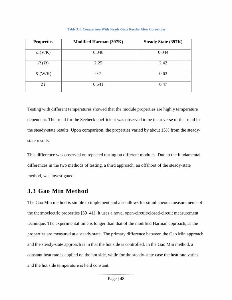
Table 3.4: Comparison With Steady-State Results After Correction

Properties Modified Harman (397K) Steady State (397K)

α (V/K) 0.048 0.044

R (Ω) 2.25 2.42

K (W/K) 0.7 0.63

ZT 0.541 0.47

Testing with different temperatures showed that the module properties are highly temperature

dependent. The trend for the Seebeck coefficient was observed to be the reverse of the trend in

the steady-state results. Upon comparison, the properties varied by about 15% from the steady-

state results.

This difference was observed on repeated testing on different modules. Due to the fundamental

differences in the two methods of testing, a third approach, an offshoot of the steady-state

method, was investigated.

3.3 Gao Min Method

The Gao Min method is simple to implement and also allows for simultaneous measurements of

the thermoelectric properties [39–41]. It uses a novel open-circuit/closed-circuit measurement

technique. The experimental time is longer than that of the modified Harman approach, as the

properties are measured at a steady state. The primary difference between the Gao Min approach

and the steady-state approach is in that the hot side is controlled. In the Gao Min method, a

constant heat rate is applied on the hot side, while for the steady-state case the heat rate varies

and the hot side temperature is held constant.

Page | 49

Figure 3.11 shows the configuration schematic. The setup has a thermoelectric module

sandwiched between a heater running at a constant heat flux and a cold plate of a fixed

temperature. All other sides are well insulated to prevent heat loss.

Figure 3.11: Schematic of the Gao Min approach

The test is first carried out in an open-circuit condition with no load. When a temperature

difference is applied across a module, a voltage is generated across it. At a steady state and when

the module is in open-circuit conditions, VOC is the voltage generated due to an applied

temperature difference of ΔTOC. The module is then short-circuited. A current due to the Seebeck

voltage flows through the specimen, resulting in additional heat flow due to the Peltier effect

[39]. As the heat flux being applied remains the same, a new temperature difference, ΔTSC, is

generated across the module.

There are four quantities that need to be measured, with the first three being the open-circuit

voltage (VOC), the open-circuit temperature difference (ΔTOC), and the short-circuit temperature

Page | 50

difference (ΔTSC). All these values are measured at a steady-state condition. To obtain the fourth

measurement, that of resistance (R), which is the voltage reading that occurs instantly upon

loading, (VL) is required.

This test is used to calculate the Seebeck coefficient and the figure of merit. To calculate the

electrical resistance, a second test is carried out using resistors of known values. As soon as the

module is loaded with a known load resistance (RL), the instantaneous voltage response (VL) of

the module is recorded. The load is immediately removed to ensure that there is no thermal

response from the module. The Seebeck coefficient ( ), electrical resistance ( ), and figure of

merit ( ) can be calculated using:

(3.27)

(

) (3.28)

(3.29)

The derivation for calculating the properties is described as follows.

Derivation

To determine the thermoelectric module properties, the measurements of VOC, VL, ΔTOC, and ΔTSC

are used. The Seebeck coefficient, thermal conductance, and electrical resistance were calculated

as per the model developed by Min [39]. Under a steady-state condition with the module at open

circuit, the voltage generated is solely due to the Seebeck effect, so

(3.30)

Page | 51

The heat rate entering the hot side (QH) is given by

(3.31)

But for an open circuit, IOC = 0

(3.32)

(3.33)

By subtracting (3.33) from (3.32), we get

0 (3.34)

When the circuit closed, the current due to the Seebeck voltage will flow through the module,

causing more heat flow across the module:

(3.35)

(3.36)

By subtracting (3.36) from (3.35), we get

(3.37)

But at a steady state, , so

(3.38)

(3.39)

The heat input is constant for both cases, so

Page | 52

(3.40)

Hence,

(3.41)

By substituting the value of α from (3.39) in (3.41),

(

)

(3.42)

[

] (3.43)

[

] (3.44)

[

( )

]

(3.45)

(3.46)

(3.47)

Hence,

(3.48)

From (3.30) we have

(3.49)

Page | 53

To calculate the resistance, a load resistor of known value is connected in series with the circuit,

as shown in Fig.3.12.

Let RL be the load resistor connected in series and VL be the voltage measured across the

thermoelectric module immediately after loading the circuit from the open-circuit state. This is

done, assuming that , where is the temperature difference immediately after

electrical loading across the module as it is loaded with the resistor.

Figure 3.12: The equivalent circuit for calculating the resistance

As the current through the circuit is the same, we get

(3.50)

(3.51)

Hence we obtain

(

) (3.52)

Page | 54

The standard equation for ZT can be written as

(3.53)

By substituting (3.45), (3.46), and (3.49) in (3.50), and solving for the conductance, we get

(3.54)

Thus, all the parameters of a TEM can be calculated using the Gao Min method using Eqns.

(3.48), (3.49), (3.52), and (3.53) by measuring , , , , , and .

Experimental setup

The setup consists of an aluminum heater block placed over the module on the hot side and a

cooling plate, which uses water as a cooling liquid, on the cold side. The aluminum block is

heated with the help of a cartridge heater that is controlled at a constant heat flux. The length and

breadth of the block are the same dimensions as the module, to minimize parasitic bypass losses.

Three thermocouples are placed in holes machined 2.5mm from the heater surface. The

thermocouples are used to verify that an isothermal heater surface is maintained. The schematic

of the setup can be seen in fig. 3.13.

Page | 55

Cold PlateDAQ

Temperature

Load ResistorSwitch S1

Switch S2

Heater

Figure 3.13: Schematic for the Gao Min approach

Voltages and temperatures are measured continuously using a DAQ system. The data obtained

from the DAQ was compiled and compared with the data from the steady-state experiments.

While the steady-state experiments were calculated applying a constant temperature difference

across the module, in this case, the heater flux was adjusted so that the hot side temperature was

maintained at 150ºC and the cold side temperature was controlled 50ºC under open-circuit

conditions. The applied loading pressure was 690 kPa. These conditions mimic those used in the

steady-state testing.

In comparing the results, the values of the figure of merit ( ) and electrical resistance differ by

10–12%, while the value for conductivity differs by almost 25%. The Seebeck coefficient is

almost the same, which can be explained by the fact that the method of calculation of the

Seebeck coefficient in both methods is the same.

It was observed that two things would improve the accuracy of the results. The first was that

better quality, well-calibrated components were necessary for accurate measurements of

Page | 56

electrical resistance. The second was that better control over the heater to maintain it at a

constant heat flux was necessary.

Correcting the first issue was comparatively simple. Off-the-shelf and better quality components

were used, and the experiment was carried with the same temperature difference (150–50ºC) and

the same applied pressure (689kPa). The results were compared as follows:

Table 3.5: Comparison of Gao Min results with Steady state ones, showing the effect of well calibrated resistors

Property Measured Gao Min Method Gao Min Method

(Calibrated)

Steady State

α (V/K) 0.045 0.046 0.044

R (Ω) 2.17 2.29 2.42

K (W/K) 0.85 0.67 0.63

ZT 0.43 0.43 0.47

The difference in results is much lower and within the acceptable range. Unfortunately,

improved control of the heat rate was not possible for the preliminary test setup. This was an area

of concern while transitioning to high temperatures. A high accuracy temperature control with

power level control was necessary to achieve the required heat rate conditions.

3.4 Conclusion

Conducting preliminary testing was necessary to better understand the practical issues of the

three different testing approaches, which in turn enabled determination of the the best approach

for module characterization at high temperatures. The major problem with the steady-state

approach is the difficulty in quantifying the heat losses to the surroundings, which will become

increasingly more challenging at higher temperatures. A secondary issue with the steady-state

approach is extremely long test times. The modified Harman method, which is based on passing

Page | 57

a current through the module, overcomes this issue, as it requires a shorter time to reach a

steady-state condition. However, the biggest drawback to the modified Harman method is that it

does not measure module parameters in actual working conditions. Another drawback is that the

adiabatic conditions required for the “heat sunk” case will become increasingly difficult to

maintain at higher temperatures.

On the other hand, the third approach using the Gao Min method was less problematic as it did

not require the heat flux to be monitored but only maintained at a constant rate. However, this

does have some of the same issues as the steady-state approaches where the heat losses to the

environment could become significant at high-temperature testing. Controlling for this can be

achieved more easily than maintaining a fixed temperature difference. Additionally, temperature

differences can be measured more accurately. The drawbacks of this approach include long

testing times and difficulty in judging whether the system has reached a steady state.

In conclusion, for high-temperature testing it was decided that a combination of the steady state

and Gao Min methods would be utilized, thereby overcoming some of the challenges of both

approaches. The new approach, called rapid steady state, is described further in the next chapter.

Page | 58

Chapter 4. Design of the Test

Apparatus

The focus of this chapter will be the thermal design of the system and description of the new

approach developed the rapid steady-state approach. The new approach was based on the steady

state, so similar limitations apply, with the most important one being accurate characterization of

heat losses. The biggest advantage of the system was very short test times. This is especially

important for long-term testing, where operating temperatures need to be maintained at a

constant over a long period of time. Based on discussions with industrial partners, specifications

for the new setup were created for successful testing of the next generation of thermoelectric

devices.

4.1 Specifications

As modules at high temperatures have not yet been developed, the laboratories working on these

modules were interested in a single setup that can accommodate a range of sizes. Prototypes

developed by them were useful in determining the expected size and arrangement of the module.

All the specifications provided are for the rapid steady-state approach.

Measurements

The measurements refer to the parameters that need to be calculated from the test. These will be

used for comparison with the module properties. The measurements of interest are:

Device level Seebeck coefficient (α)

Device level overall electrical resistance (R)

Page | 59

Device level overall thermal conductance (K)

Peak power (Pmax)

Uncertainty

Uncertainty in a measurement is a parameter associated with the result of a measurement that

characterizes the dispersion of the values that could reasonably be attributed to the quantity of

interest [52]. In this case it is defined as an estimate of the error in the measurement stated as a

range of values that contain the true value within a certain confidence level.

Seebeck coefficient: +/–5%

Electrical resistance: +/–5%

Thermal conductance: +/–10%

Peak power: +/–5%

The uncertainty in thermal conductance is assumed to be higher owing to the high uncertainty in

power measurements.

Device sizes

The size range was taken directly from the laboratories. Forty millimeters was decided as the

upper limit to accommodate low temperature validation for the module.

1–20 leg pairs (note there is no characterization of a single leg)

5–14mm device thickness (3–10mm leg lengths with 1–2mm substrates)

4–40mm device side lengths

Page | 60

Temperatures and environmental conditions

All isothermal surfaces within +/–1°C

Hot side temperature to be controlled from 100–650°C

Cold side temperature to be controlled from 50–550°C

No vacuum is required, but the ability to have a fully inert environment (i.e., argon or

nitrogen purged) is necessary

All temperatures are to be controllable to within 20°C

4.2 Build Overview

The greatest difficulty in testing the modules at the specified temperatures is the measurement of

heat rates. A couple of alternatives were described in the literature review, with the first one

being characterization of heat losses. At high temperatures, the radiation losses become

dominant. These are very difficult to characterize, especially the surface-to-surface radiation

component, which result in a large measurement uncertainty.

Another option is to use a heat meter in the form of a reference material placed in the path of the

heat flow. This method has better accuracy and a comparatively lower uncertainty, but is not

without issues. The biggest problem is the inherent uncertainty in published values of reference

materials. Even for well-researched materials, the standard deviation in values is 5–10%.

Calculating exact heat fluxes using a reference material relies on the measurement of the exact

temperature difference along the sample length. Even the most reliable thermocouples have an

uncertainty of ±2°C. This uncertainty propagates through to the heat flux measurement.

The last difficulty is predicting heat losses from the reference material. This can be minimized by

placing the reference material or heat meter on the cold side so that losses are reduced. It was

Page | 61

decided that this method would be incorporated into the setup on the cold side as a check in the

measurement of the heat flux, but not as the main source of heat flux measurement.

To overcome the potential errors of the above two approaches, a guard heater arrangement as

described by Rauscher et al. [36,37] is used in the system. A guard heater arrangement is

basically a smaller heater surrounded by a larger heater. The only exposed surface of the main

heater is the face in contact with the thermoelectric module. The remaining sides of the main

heater are enclosed by a guard heater. The main and guard heaters are maintained at the same

temperature so that, theoretically, there will be no temperature difference between the main

heater and guard heater and therefor no heat loss from the main heater block to the guard heater

block. This also ensures 1-D conduction from the main heater to the module.

To enable control of the cold side of the module, a cold side heater arrangement is developed.

This are explained in detail in sections 4.3 – 4.5.

Figure 4.1 depicts an overall schematic of the developed system. A thermoelectric module (4) is

sandwiched between two heater blocks that maintain the temperatures on the hot and cold sides.

Each heater block consists of a base heater (2) and swappable extension plate (3 and 5) to

accommodate different-sized modules. The guard heater (1) surrounds the hot side heater block,

ensuring 1-D conduction and eliminating heat losses from the main heater block. On the cold

side, the cold side heater block (5) is connected to a spacer (6), which is connected to a water-

cooled chiller plate (7). The assembly is supported on four linear bearings. Both heater blocks

are insulated using alumina silica ceramic. A load cell (8) measures the pressure applied on the

module by a hand crank (9).

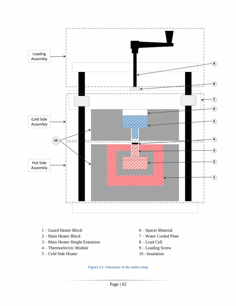
Page | 62

Cold Side Assembly

Hot Side Assembly

Loading Assembly

1

2

3

4

5

6

7

8

9

10

1 – Guard Heater Block

2 – Main Heater Block

3 – Main Heater Height Extension

4 – Thermoelectric Module

5 – Cold Side Heater

6 – Spacer Material

7 – Water Cooled Plate

8 – Load Cell

9 – Loading Screw

10 - Insulation

Figure 4.1: Schematic of the entire setup

Page | 63

4.3 Thermal Modeling

In order to quantify and then minimize the losses from the main heater block and ensure

isothermal surfaces for a range of thermoelectric modules that might be tested, a thermal model

of the concept system was developed. What follows is a description of the models developed for

the various subsystems of the concept test stand.

Main heater assembly

The size of the main heater was decided upon by keeping in mind the maximum size of the

module to be tested. As proof of concept, the existing modules, which have been previously

categorized, will be tested on the setup. The size of these modules is 40mm x 40mm. Hence, the

size of the main heater block is 40mm x 40mm x 20mm. The height selected will ensure an

isothermal surface in contact with the module. Discussions with our industrial partners helped to

identify a range of physical dimensions of the new modules, which the setup should be able to

accommodate. Based on these values, four extreme cases were studied, and the specifications

were developed. According to the dimensions, the device thickness could vary from 3–14mm

and the number of leg pairs would vary from 1–20. When the module is not the same size as the

heater, a small extension will be attached to the surface of the heater. The guard heater plate will

surround the smaller extension, as shown in Fig. 4.4.

This configuration ensures that the heat from the heater flows only to the module and that there

are no other losses. This extension will be thermally coupled with the heater and will be made of

the same high-conductivity material. Consequently the surface of the extension block will also

remain isothermal.

Page | 64

The setup is designed to test a thermoelectric module that contains multiple thermoelectric leg

pairs. Going by this definition, the smallest thermoelectric module that can be tested by the setup

would contain at least one leg pair. Testing of individual legs will not be possible. Feedback

from the laboratories developing these modules helped define the size of each leg as 2mm x

2mm. Thus, the minimum size of the module that can be tested will contain one leg pair, with

each leg having a 2mm square side. The overall size of the module can be varied by increasing

the gap between the legs. The maximum size of a module that will be developed in the near

future was estimated to have 20 leg pairs, also with each leg having a square side of 2mm.

Another limiting factor is the amount of current flowing through the system. High currents

require expensive instrumentation, increasing the overall cost. As the leg pairs are electrically in

series, the number of leg pairs does not affect the total current. The thickness or length of the

legs is inversely proportional to the current flowing through them. Thus, the shorter the leg, the

more the current flowing through it, assuming the area of each leg is constant. By keeping the

maximum allowable value of the current as 15A, the minimum leg length for testing was

calculated as 3mm.

The leg length also affects the amount of heat flowing through it—the longer the leg, the lower

the heat rate flowing through it. For a particular temperature difference, the heat losses from the

main heater block can be assumed to be constant regardless of the module size. As the leg length

increases, the heat rate through the module becomes so low that they almost equal the heat losses

from the main heater block. This leads to large uncertainties in the measured values. To avoid

this situation, the maximum length was capped at 10mm.

Based on these values, the four extreme cases were considered:

Page | 65

Case A: 1 leg pair with 3mm leg length

Case B: 20 leg pairs with 3mm leg length

Case C: 1 leg pair with 10mm leg length

Case D: 20 leg pairs with 10mm leg length

For all cases, the dimensions of each leg were 2mm x 2mm.

To model the heat flux requirement of the main heater, the properties required were the thermal

conductivity ( ) and the physical dimensions of the thermoelectric module. The module level

Seebeck coefficient and the module level electric resistances were also calculated by using the

Seebeck coefficients of the individual leg pairs ( ) and the electric resistivity ( ).

The schematic of the thermoelectric leg pair is shown in Fig. 4.2.

Ceramic Plate

Electrical Interconnects

P leg N leg

Ceramic Plate

The

rmal

Byp

ass

Figure 4.2 Schematic of a thermoelectric leg pair

Page | 66

Modeling

The heat flux calculation was done using the thermal resistances of the individual components of

the thermoelectric module. The components formed a circuit, as shown in Fig. 4.3.

R ceramic

R interconnects

R p- type R n- type

R bypass

R ceramic

R interconnects

Figure 4.3: Thermal circuit of the module

Thermal resistances

1. Ceramic plate

To calculate the thermal resistance of the ceramic plate, the thermal conductivity was assumed to

be 22W/mK. The dimensions of the plate were calculated assuming a 50% fill ratio, which

Page | 67

means that 50% of the module area was covered with thermoelectric material, while the

remaining 50% was an air (or inert gas) gap. The length was assumed to be a constant of 1mm.

The thermal resistance of the ceramic plate is

(4.1)

2. Electrical interconnects

The interconnect material was assumed to be copper with a conductivity of 370W/mK. The

dimensions of the substrate were also calculated using a 50% fill area, with a constant thickness

of 0.5mm.

(4.2)

3. Leg pairs

Using the material properties provided, the thermal resistances of the legs were calculated:

(4.3)

(4.4)

where the subscripts and represent positive-majority-carrier doped and negative-majority-

carrier doped materials respectively.

4. Thermal bypass

Thermal bypass is the amount of heat that flows through the gaps between the leg pairs. As the

gap is very small, there will be no heat transfer due to convection. But radiation and conduction

Page | 68

will be present in parallel. Using the conductivity of argon, the thermal resistance can be

calculated as

(

)

(

)

(4.5)

where and are emissivities of the two surfaces, assuming a large parallel-plates case.

Using the thermal circuit from Fig. 4.3, the overall thermal resistance is calculated as

(

)

(4.6)

The module level conductance can be calculated as

(4.7)

The module level Seebeck coefficient is calculated as

(4.8)

And the module level resistance is calculated as

[(

)

(

) ] (4.9)

Using the power equation for a module,

(4.10)

Dividing both sides by the current ( ), the module voltage can be obtained:

(4.11)

Page | 69

Thus, for an open-circuit condition,

(4.12)

For a short-circuit condition, substitute in Equation (5.10). Thus,

(4.13)

From Eqns. (5.11) and (2.7), the heat entering the module in a short-circuit condition is

⁄ (4.14)

This is the heat flux in a short-circuit condition, assuming a constant temperature difference.

If we substitute I = 0, which is the open-circuit condition, the heat entering the module is then

(4.15)

Assuming that the module operates from 923K at the hot side to 373K at the cold side, the heat

flux for the two extreme cases in short and open circuits can be obtained, then used to explore

the range of heat rates needed and the relative impact of error in the main heater power losses.

Using Eqns. (4.7) - (4.9) and (4.12) - (4.15), module parameters can be determined as well as the

range of required heat transfer rates to maintained the desired temperature differences for the

four extreme cases of thermoelectric modules that might be tested in the current setup. The

material properties used for this simulation can be seen in table 4.1.

Page | 70

Table 4.1: The Material Properties Used in Simulation of Extreme CasesTable

Property p-type n-type

(V/K) 1.26E-04 -1.68E-04

(Ω-m) 1.0E-05 1.0E-05

(W/m-K) 1.5 1.5

The results are summarized as seen in Table 4.2.

Table 4.2: Properties of Four Extreme Sizes of Thermoelectric Modules

Parameter A B C D

α (V/K) 0.00029 0.0059 0.00029 0.0059

R (Ω) 0.015 0.3 0.05 1

K (W/K) 0.004 0.08 0.001 0.03

(W) 4.30 86.08 1.38 27.53

(W) 2.25 45.01 0.76 15.21

I (A) 10.78 10.78 3.23 3.23

(V) 0.16 3.23 0.16 3.23

The values of the current, voltage, and heat rates provide a basis for selection of instrumentation

and heaters. Even though the voltages are quite small, the currents can be quite large for some

modules.

Guard heater assembly

In the previously published literature, the guard heater was used to mainly minimize losses from

the base of the guard heater. The losses through the size were assumed to be negligible by

making the main heater as thin as possible. Even though this is a good approximation, it could

lead to large errors at high temperatures. In the new system, the guard heater block covered all

Page | 71

sides of the main heater block. The proposed shape of the heater is shown in Fig. 4.4. The guard

heater block is divided into four zones, depending upon its orientation and the materials with

which it is in contact. Zone 1 is the base of the guard heater block, Zone 2 constitutes the sides,

Zone 3 is the top plate of the guard heater block with the outer surface in contact with the

insulation over the cold plate, and Zone 4 is the part of the guard plate exposed to the cold side

heater through the insulation.

Insulation is present on both the inside and outside surfaces of the guard heater. The insulation

on the inside will reduce thermal coupling of the guard heater and the main heater, which will

reduce the heat loss to the guard heater block. The insulation on the outside will prevent

excessive losses to the environment and therefore reduce the required guard heater power, as

well as ensure more uniform temperatures throughout the guard heater.

Page | 72

Cold Plate

Insulation

Conduction

Conduction

Ambient (Qa)

Main Heater

(Qh)

Zone 1

Zone 2

Zone 3

Zone 4

Figure 4.4: Guard heater schematic showing the various zones. Also shown is the discretization method of the guard

heater

The overall dimensions were based on the insulation used as well as the material of the heater. A

simulation in Excel was used to obtain the dimensions and an estimate of the losses, followed by

a COMSOL and ANSYS simulations to predict the heat losses. With the Excel simulation, a

finite difference method was used to calculate losses along the length of the guard heater. The

fluxes were calculated for each section of the guard heater, then summed up.

For the analysis, it was assumed that the guard heater element was conducting heat to and from

its adjoining elements and simultaneously losing heat to the main heater as well as the ambient

Page | 73

environment. Each element was assumed to be isothermal and constant conductivities and a

steady state for the entire system was assumed. To calculate the heat lost to the ambient

surroundings, the thermal circuit shown in Fig. 4.5 was used.

Tinsulation

Rinsulation

Rradiation

Rconvection

Theater

Tambient

Tambient

Figure 4.5: Thermal circuit for calculating insulation losses

Insulation losses for each discrete section are calculated by

( )

( )

(4.16)

where ( ) (

)

(

) (4.17)

where

(4.18)

( )

(4.19)

where (

)

(4.20)

Furthermore, to keep the simulation 1-D, certain assumptions were made. It was assumed that for

the entire length of the guard heater, heat would be lost to the surroundings from the outer

Page | 74

surface and there would be heat gain from the main heater at the inner surface. The second

assumption was that the base of the guard heater is isothermal, and is the same temperature as the

main heater. Thus, there is no heat lost from the main heater to the top part of the guard heater.

The contact resistance between the guard heater block and the top plate was assumed to be

negligible. These assumptions make the simulation a little liberal. To compensate for this, it was

assumed that the main heater block is isothermal along its length, effectively overestimating the

heat losses. This assumption is valid for heater materials of high conductivity.

A simulation was run for an extreme case where the module is at 923K on the hot side and 373K

on the cold side. The module selected was with a single 4mm x 4mm x 10mm leg pair. It was

observed that for this case, almost 30% of the main heater power was being lost to the guard

heater. A simple fix to this is to maintain the guard heater block at a higher temperature than that

of the main heater block. The results obtained by holding the guard heater block at 1°C higher

than the main heater block can be seen in Table 4.3.

Table 4.3: Heat Losses Calculated (to the Main Heater and to Surroundings)

(W) (W)

Zone 1 0.13 18.61

Zone 2 -0.04 55.05

Zone 3 -0.09 13.91

Zone 4 -0.03 8.86

Total -0.03 96.44

The negative sign for indicates that heat is gained by the guard heater. For the above case, the

losses dropped to 2% when the guard heater was held at a higher temperature. Also, as expected,

the heat loss to the main heater is much smaller than the heat loss to the environment. In the

Page | 75

subsequent sections, the heat flux required for such a small thermoelectric module is also

calculated.

The simulation helped to determine the dimensions of the guard heater and the insulation. In the

insulation design, the outer part was not as critical as the inner insulation. It was initially planned

to have no insulation between the main and the guard heater blocks. This worked well at low

temperatures, but as the temperature increased radiation losses also increased. Placing insulation

between the two heater blocks made the radiation losses negligible. The thickness of the outer

insulation was governed more by the overall mechanical design rather than the thermal design. A

thickness of 20mm was selected for the outer insulation to maintain a safe outside surface

temperature and keeping in mind the various design aspects.

For the inner insulation, it was observed that for thicknesses over 8mm, the radiation losses

without the insulation were greater than conductive losses through the insulation. A 10mm

thickness was selected for the inner insulation. Another advantage of insulating the inner surface

is that the position of the main heater is secured.

There were two main objectives in selecting a thickness for the guard heater: the heat losses to

the ambient environment should be as low as possible, and the temperature gradient along the

length of the guard must be as low as possible. However, these objectives contradict each other.

As the size of the guard heater block decreases, the heat losses to the ambient surroundings also

decrease, so it is desirable to make the guard as small as possible. But as the guard becomes

smaller, the temperature gradient along the length increases. This not only contradicts the second

objective, but also increases the heat loss from the main heater to the guard. To optimize both

objectives, a thickness of 15mm was selected for the guard heater.

Page | 76

The dimensions of the insulation and guard heater obtained from this simulation were used as a

starting point for further analysis.

Cold side heater assembly

The cold side heater assembly includes the cold side heater, a spacer, and a liquid-cooled cold

plate. A spacer is basically a block made of a material with enough thermal resistance that the

liquid in the cold plate (water) stays below its boiling point. The spacer is designed for the

expected heat rate exiting the cold side of the module under short-circuit conditions. This will

ensure that the cold side heater is held at the required temperature even in the short-circuit

condition. For the above case, ( = 973K and = 373K), the cold plate was assumed to be

at 323K ( ). The assembly can be seen in Fig. 4.6.

The thermal resistance of the spacer can be calculated as

(4.21)

Cold Heater

Spacer

Cold Plate

Qc

Tc

Tcp

Figure 4.6: Cold side heater assembly

Page | 77

One drawback of the spacer design is that it is designed according to a fixed temperature

difference. As the temperature difference changes, the cold side heater will have to compensate

for the difference in heat flux. This can be seen in Table 4.4. The table is for the extreme module

case under different operating temperature differences.

Table 4.4: Cold Plate Heat Flux for Different Temperature Differences

Case A

(K) 923 923 473

(K) 373 823 373

SC (W) 4.30 0.91 0.65

SC (W) 0.00 42.13 3.65

(W) 4.30 43.04 4.30

There is a large increase in the heat rate when the cold side temperature approaches that of the

hot side. To accommodate such a large range, spacers of different thermal resistances will be

needed. This can be achieved by varying the material of the spacer.

4.4 COMSOL and ANSYS Models

A numerical study was conducted in COMSOL and ANSYS to verify the values from the simple

1-D approach described above. A second objective was to verify that the surfaces adjacent to the

thermoelectric module are isothermal.

Modelv

The overall dimensions for the guard heater, main heater, and insulation were taken from the

preliminary model. The thermoelectric module was assumed to be 4mm x 4mm x 4mm. As

stated earlier, the main heater was 40mm x 40mm x 20mm. The guard heater has a base

Page | 78

thickness of 20mm and a side thickness of 15mm. The top plate of the guard heater is 10mm

thick and surrounded by high-temperature insulation of 20mm on all sides. The cold side

insulation is 30mm to accommodate the cold side heater and the spacer. The insulation between

the main heater and the guard heater was 20mm.

Materials

There were three different materials used in the simulation: the heater material, the insulation

material and the spacer material.

To determine the best heater and guard heater materials, a material search was conducted, which

resulted in nine options, shown in Table 4.5. The main criteria for selection are the three

properties of thermal conductivity, specific heat, and density. The most important property

required for the heater material is thermal conductivity. Because the heater blocks would be

heated with the help of cartridge heaters, high conductivity will help reduce the temperature

difference across the heater blocks and the height extensions. Secondly, as an important part of

the experiment is based on the transients of the system, low specific heat and low density are also

essential.

In the table, the maximum temperature refers to the maximum operating temperature of the

materials without oxidization. Where oxidization temperatures were unavailable, the melting

temperatures denoted by (MP) are stated.

Page | 79

Table 4.5: Material Options for Heaters

Name

Conductivity Sp Ht Max Temp Density

W/mk J/kgK °C kg/m3

Potovell II: machinable nitride [53] 50 - 1000 2560

Aluminium nitride [54,55] 170 740 800 3260

Copper [56] 380 384.4 400 8960

Nickel [57] 91 445 1450 8908

Boron nitride [58] 71 1470 1300 1900

Silicon carbide [59] 120 750 1400 3100

Molybdenum [60] 139 251 800 10280

Beryllium oxide (Berlox) 265 1047 1800 (MP) 2850

Beryllium copper [61] 144 419 1100 (MP) 8800

With the complex geometries that need to be machined, coupled with machining ease and cost,

copper was the best candidate. Unfortunately, copper does have oxidation properties at elevated

temperatures. Copper starts oxidizing around 400°C and readily oxidizes above 500°C [56,62],

limiting the range of testing temperatures. Thus, this was selected only for the first prototype of

the setup, which would be used for low-temperature validation. For testing at 650°, the best

choice of material was aluminum nitride owing to its high conductivity and relative ease of

machining.

For the insulation material, cost and ease of machining were the two main criteria for selection,

apart from the operating temperature. Alumina silica ceramic foam was selected, which has an

operating temperature of 1650°C. It is easily machined and resistant to oxidization within its

Page | 80

operating temperature range. The spacer material was selected using the simulation. Stainless

steel was selected as the material as it was the closest to the requirement in terms of thermal

conductivity.

Boundary conditions

The material properties for copper and stainless steel were taken from the built-in materials

library in COMSOL. The properties for the insulating materials were taken from the values

provided by Cotronics Corp. for alumina silica ceramic. The material properties for the

thermoelectric module itself, especially the conductivity, were calculated using the module level

conductance from the preliminary model. Temperature boundary conditions were applied on the

main heater block, guard heater block, and the cold heater block. The main heater and the guard

heater were held at 923K and the cold heater at 323K. All the external surfaces of the insulation

were assumed to be losing heat to the environment via convection and radiation. An overall heat

transfer coefficient of 5W/mK and a surface emissivity of 0.5 was assumed.

Mesh

The results in COMSOL are extremely sensitive to the mesh size: the finer the mesh, the more

accurate are the results. But as the mesh becomes finer, the computational time also significantly

increases. To reduce the number of elements in the mesh, only half of the model was used for the

simulation. Unfortunately, because there is a large variation in the sizes of the components of the

setup, the number of elements in the mesh is numerous. Based on the resources available, only a

medium overall mesh was possible, because of the high computational time required for

rendering the fine meshes. To optimize resources, the local mesh for the heater height extensions

and the thermoelectric module were made to be fine.

Page | 81

Post-processing

The problem was set up to simulate the working of a 4mm x 4mm module, operating at 923K on

the hot side and 373K on the cold side. The solver selected was the standard generalized

minimum residual (GMRES) solver, with 10,000 iterations and a termination damping factor of

1E-6. The resulting thermal contours can be seen in Fig. 4.7. Post-processing was useful in

determining whether the surfaces were isothermal and calculating the heat losses.

The first step confirmed that the surfaces were isothermal, using the surface min and surface max

functions for temperature. The values obtained for the hot side were 922.88K as the minimum

and 923.27K as the maximum, giving an uncertainty of 923.1 ± 0.2°C. For the cold side, the

minimum temperature was 373.27K and the maximum was 373.97K, giving an uncertainty of

373.6 ± 0.4°C. This is within well our specification of ±1°C.

The calculation of heat flux was slightly trickier. Due to the way the finite element method

calculates the result, there is a significant error caused when the geometry domain changes shape

drastically.

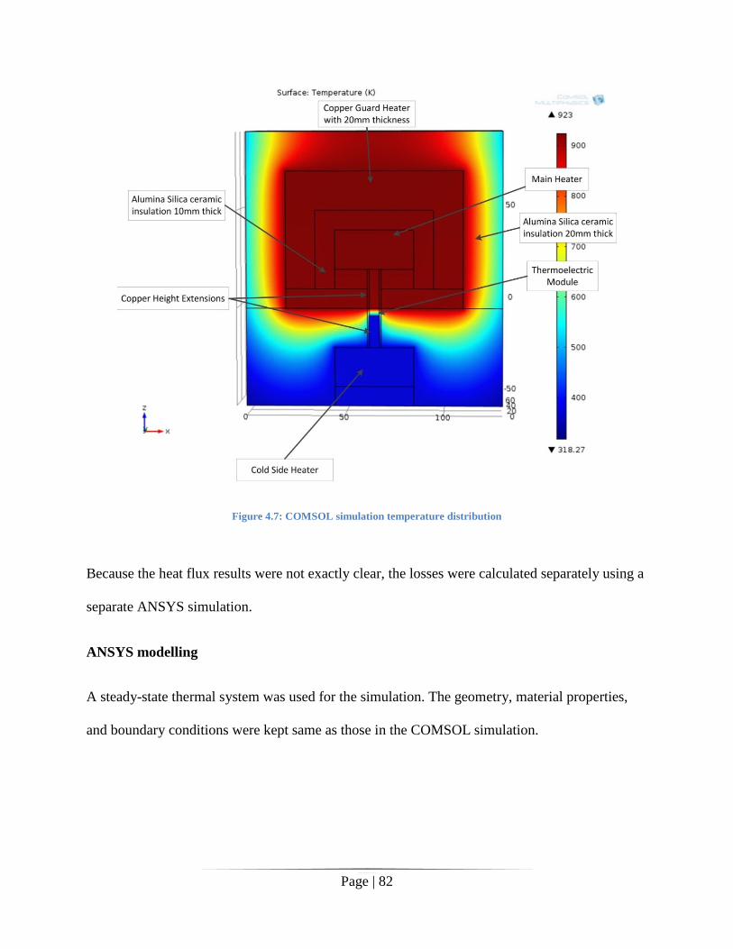
Page | 82

Figure 4.7: COMSOL simulation temperature distribution

Because the heat flux results were not exactly clear, the losses were calculated separately using a

separate ANSYS simulation.

ANSYS modelling

A steady-state thermal system was used for the simulation. The geometry, material properties,

and boundary conditions were kept same as those in the COMSOL simulation.

Page | 83

Figure 4.8: Temperature distribution across the main heater

Even at 923K, the surface of the height extension is isothermal within 0.5°C. Analysis performed

on the main and guard heater assemblies indicated a temperature gradient of less than 8°C across

the entire guard heater block under the worst case conditions, specifically when the hot side

temperature is 650˚C and the cold side temperature is 50˚C. These temperature profiles were

compared with those from the COMSOL simulation to calculate the heat losses from the main

heater. Under this extreme case, the maximum heat transfer between the main heater block and

guard heater was less than 2% of the heater power.

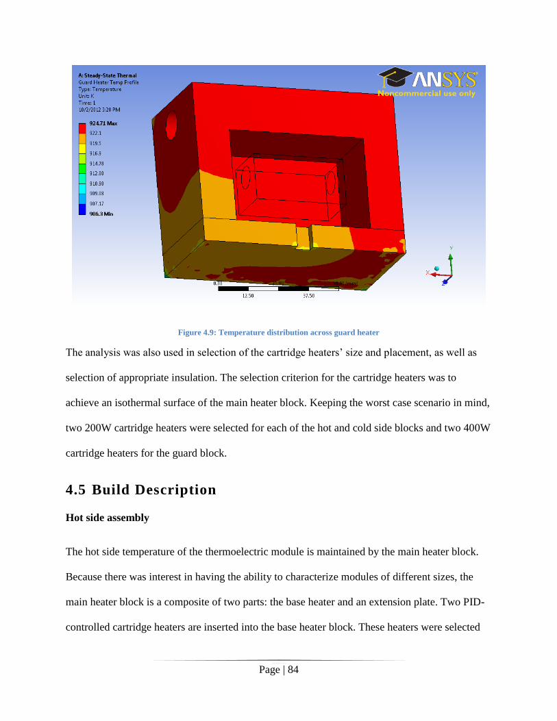
Page | 84

Figure 4.9: Temperature distribution across guard heater

The analysis was also used in selection of the cartridge heaters’ size and placement, as well as

selection of appropriate insulation. The selection criterion for the cartridge heaters was to

achieve an isothermal surface of the main heater block. Keeping the worst case scenario in mind,

two 200W cartridge heaters were selected for each of the hot and cold side blocks and two 400W

cartridge heaters for the guard block.

4.5 Build Description

Hot side assembly

The hot side temperature of the thermoelectric module is maintained by the main heater block.

Because there was interest in having the ability to characterize modules of different sizes, the

main heater block is a composite of two parts: the base heater and an extension plate. Two PID-

controlled cartridge heaters are inserted into the base heater block. These heaters were selected

Page | 85

such that the surface in contact with the thermoelectric module is isothermal. It is assumed that

the entire power input to the heater is passing through the module. Compared to measuring heat

flow, measurement of electric power is much easier, and precise measurement of the output from

a module is possible [38]. In order to accurately determine the heat flow through the module and

to ensure 1-D conduction, it is imperative that the heater extension plate be the same size as the

module. The extension plate is customized for each module and is attached to the main heater

block, and allows for testing of 4 mm x 4 mm to 40 mm x 40 mm thermoelectric modules using

the same base heater. The heater block was made of copper with a flatness of 0.05mm.

Figure 4.10: Main heater assembly

Because of its high thermal conductivity, copper was selected as the heater block material to

ensure isothermal surfaces, ready availability, and ease of machining. Due to oxidation problems

at higher temperatures [62], the next generation of the test stand will use boron nitride or AlN as

the heater block material; both of which are stable up to 800˚C in air. Type K thermocouples,

composed of chromel/constantan alloy and the most commonly used general-purpose

Page | 86

thermocouples, were used for all temperature control and measurements. These are stable in air

or inert atmosphere up to 1260°C, have reasonable uncertainty, and are inexpensive.

1

2

3

4

5

6

7

Figure 4.11: Sensing thermocouple placement in setup

Figure 4.11 depicts the placement of the sensing thermocouples in the setup. Thermocouples 1

and 2 measure the temperature gradient across the length of the main heater block.

Thermocouple 2 is 2.5mm from the surface that contacts the module. Based on the heater power,

a correction factor is applied to account for the temperature difference across the distance

between the sensor and the surface. Thermocouples 3 and 4 measure the temperature difference

along the length of the cold heater and are similarly corrected using correction factor.

Thermocouples 6 and 7 measure the difference across the guard heater. Thermocouple 5 was

placed in the guard plate to quantify any contact resistance between the guard heater block and

the guard cover plate.

Page | 87

Figure 4.12 depicts the placement of the control thermocouples in the setup. Thermocouple A

controls the temperature of the main heater, and is placed close to the heater cartridges to ensure

that there is no temperature difference between the cartridges and the thermocouple.

Thermocouples B and C are the guard heater control thermocouples. They are connected in a

closed loop, and control the temperature of the guard heater by maintaining a constant

temperature difference between the two thermocouples. Thermocouple D controls the

temperature of the cold side heater and is also placed close to the heater cartridges.

Thermocouples E and F are emergency shutoff thermocouples and are placed on the main heater

block and the cold plate. These are safety thermocouples, which shut down all power to the

heaters if the temperature limit is reached. The hot side temperature limit is set to 450°C for

preliminary testing, and the cold side temperature limit is 70°C to avoid boiling of the water.

A B

D

C

E

F

Figure 4.12: Control thermocouple placement in setup

Page | 88

Guard heater assembly

The guard heater, also made of copper, is shaped as a hollow cube, with a uniform thickness of

15mm around the sides and 20mm at the base, as seen in Fig. 4.12. It is mounted on the

aluminum base with the help of four ANSI-304 screws, which are 20.5mm long. The screws help

to secure the location of the guard heater block and also help to protect the insulation from

breaking due to the thermal expansion of copper. The gap between the main heater block and the

guard heater block is filled with alumina silica insulation to minimize thermal coupling, which is

primarily due to radiation.

The top plate of the guard heater can be interchanged to facilitate different main heater extension

sizes, and is sized so that the gap between the main heater extension and the plate is 1.5mm on

each side. Thermocouples are placed along the length of the guard heater to calculate the

temperature difference across the guard.

The guard heater arrangement was selected to achieve two main goals: to maintain an isothermal

top surface of the main heater block and to prevent heat loss from the main heater block. During

the experiment, a gradient of 2°C across the length of the guard was observed when the hot side

temperature was maintained at 200°C and the cold side at 50°C. Due to this difference, there is a

heat loss from the main heater block to the guard heater block. A suitable correction factor

accounts for this loss while calculating the main heater power output. Because the heaters are

most thermally coupled at the top plate, care was taken to maintain the top of the guard and main

heater at the same temperature.

Cold side assembly

Page | 89

To enable control of the cold side of the module temperature between 75°C and 550°C, another

heater block was placed on the cold side, similar in configuration to the main heater. The only

difference between the hot and cold side heaters is that the height of the cold heater extension

plate was adjusted to accommodate the thickness of the module. Modules varying from 2mm to

18mm thick can be tested. The size limits are stated keeping in mind the specifications provided

by the manufacturers of the module. In reality, the setup can accommodate much thicker

modules. A lower-conductivity spacer material, stainless steel, was placed between the heater

and the water-cooled chiller plate to help maintain an appropriate thermal difference.

Like the hot side heater, two PID-controlled cartridge heaters were inserted into the heater block.

Thermocouples 3 and 4 (Fig. 4.12) were placed at 10mm distance from each other with

Thermocouple 3 being 2.5mm from the top of the cold heater block. These were used as a second

method of measuring the heat rate passing through the module. In open-circuit conditions, the

heat rate transferred to the module is equal to the heat rate leaving the module, which is

measured using the thermocouples spaced at a known distance in a material with known thermal

conductivity. This provides an additional check when calculating the heat rate.

Loading assembly

One of the important issues in module testing is to maintain a constant and even loading pressure

and full surface contact across the entire thermoelectric surface. Four linear bearings guide the

cold side assembly so that there is complete contact between the module and the heaters. The

cold side assembly is supported by springs. The contact pressure is an important criterion to

ensure repeatability in testing: therefore, a load cell is used to measure the pressure applied on

the module. The movement of the assembly is controlled with the help of a threaded lead screw

Page | 90

that rests on the load cell. During the experiment it was observed that the optimal loading

pressure is at or above 700kPa.

Inert environment

Testing in an inert environment is required for this stand, due to the susceptibility to oxidation

exhibited by some high-temperature thermoelectric materials being considered for power

generation devices. The stand was designed to be installed in a sealed enclosure to facilitate

nitrogen or argon purging. The design incorporates the ability to easily remove the test stand

from the enclosure for maintenance and to change the heater extensions.

There are four important parts: the enclosure, the gas tank, a pressure regulator, and an exhaust

valve. The general schematic of the system can be seen in Fig. 4.13.

P

Gas Tank

Two stage pressure regulator

Air tight enclosure

Exhaust port with screw

valve

Figure 4.13: Schematic of the argon purging system

Page | 91

The figure shows an inert gas tank (either argon or nitrogen) connected to an airtight enclosure

via a two-stage pressure regulator. Argon is preferred over nitrogen because of its purity.

Nitrogen is generally produced by reverse osmosis of air and as such can contain some traces of

oxygen, which may cause oxidation of the thermoelectric module. Another advantage of argon is

that it is heavier than air. This reduces the number of air changes required to set up the inert

atmosphere for testing. The two-stage pressure regulator converts the high-pressure liquid (over

400 psi) from the gas tank to low-pressure gas (about 3 psi) required at the enclosure. The inlet

port for the argon gas is connected near the base of the enclosure, causing the lighter air inside

the box to move to the top. An exhaust port consisting of a screw valve is attached near the top

of the enclosure. This is used to exhaust any air inside the enclosure.

Of the four parts, the most important is the enclosure and it should meet the following criteria:

The enclosure should be airtight so that gas does not leak; the steel grade should be high enough

to withstand the internal pressure; the enclosure must be sturdy enough to allow passage of

multiple electrical and plumbing connections through the wall; and it should be able to withstand

~80°C without failure. The enclosures that satisfy all these conditions fall into two categories,

desiccators and NEMA boxes. Desiccators are basically industrial dryers that can withstand up to

250°C and have a large range of gas flow speeds. Their primary purpose is to purge

nitrogen/inert gas. Although very well suited for the application, there is significant difficulty in

making external connections. Thus, these have to be mostly custom-made by the manufacturer,

raising the cost.

NEMA boxes are mainly electrical boxes available in various grades, with the airtight/watertight

grade being NEMA 4/4X. These boxes come lined with a gasket material on the inside of the

doors that will reduce leakages from the box. The NEMA 4 boxes are also made of 16-gauge

Page | 92

galvanized steel, so it can easily handle the resultant pressure. Additionally, they are easily

customized post-purchase, and also have a viewing window to check for any leaks in the system.

Keeping these factors in mind, a NEMA 4 enclosure of dimensions was

purchased. For electrical and water connections a side plate was mounted, with cutouts for the

various connections. The side plate can be seen in fig. 4.14.

Figure 4.14: Inert gas purging enclosure

Page | 93

4.6 Troubleshooting

Base plate

The guard heater is supported on the base plate with the help of standoff screws. Even though

these are made up of ANSI steel, which has a comparatively low thermal conductivity, the

thermal coupling of the guard heater and the base caused the base plate to heat up. To avoid this,

the base was fitted with a rectangular finned base. The fins selected ran along the entire length of

the base plate. This reduced the temperature considerably to safe levels by increasing the heat

dumped to the air. Figure 4.15 shows the standoffs the guard heater is mounted on, as well as the

finned base attached.

Figure 4.15: Guard heater arrangement with finned base

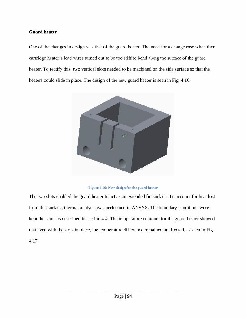
Page | 94

Guard heater

One of the changes in design was that of the guard heater. The need for a change rose when then

cartridge heater’s lead wires turned out to be too stiff to bend along the surface of the guard

heater. To rectify this, two vertical slots needed to be machined on the side surface so that the

heaters could slide in place. The design of the new guard heater is seen in Fig. 4.16.

Figure 4.16: New design for the guard heater

The two slots enabled the guard heater to act as an extended fin surface. To account for heat lost

from this surface, thermal analysis was performed in ANSYS. The boundary conditions were

kept the same as described in section 4.4. The temperature contours for the guard heater showed

that even with the slots in place, the temperature difference remained unaffected, as seen in Fig.

4.17.

Page | 95

Figure 4.17: Thermal analysis on redesigned guard heater

Linear bearings

The linear bearings selected earlier were self-aligning bearings that had an allowable shaft

misalignment of 1/2˚ in any direction. The combined effect of four such shafts resulted in the

cold plate assembly not remaining perfectly horizontal while lowering. The perfect alignment of

the cold plate assembly with the main heater was critical in the setup. To overcome this, a fixed

alignment bearing was selected and installed.

Main heater assembly

The main heater consisted of two parts: the heater block into which the cartridge heaters were

inserted, and the height extension plate, which was screwed in to the heater block. The

arrangement was selected so that different module sizes may be tested using the same setup and

only switching out the height extension plate. The main heater block was designed to use size 0-

80 screws, which resulted in the maximum allowable size of the module to be 32mm. Due to the

Page | 96

physical constraints of copper, the 0-80 screws were switched to 4-40s. The larger screws

reduced the maximum allowable size of module to 27mm.

Spacer material

In order to maintain the cold side at the required temperature, a spacer material was introduced

between the cold plate and the cold heater. Analysis suggested selecting a material of thermal

conductivity of 15W/mK. Thus, stainless steel, which has a comparable thermal conductivity of

16.23W/mK, was selected. Unfortunately, contact resistance was not taken into account in the

analysis. Because of the large contact resistance between the surfaces, a higher conductivity

material was required. For low-temperature testing, an aluminum spacer was selected.

Guard heater plate

After seeing the effects of contact resistance, it was decided to test for the same effects on the

interface between the guard heater and the guard plate. A thermocouple was placed just below

the plate and another was placed in the plate itself. Had there been a presence of a large contact

resistance, a significant temperature drop would be expected across it. However, after running

multiple tests, the temperature difference was observed to be less than 1˚C when the guard heater

was held at 200˚C and the cold side was held at 70°C.

Heater controls

The control thermocouples for the main and guard heater blocks were near their respective

cartridge heaters. As the main heater was in contact with the thermoelectric module, a

temperature drop was developed from the control thermocouple to the sensing thermocouple,

which was placed very close to the surface. In order to maintain the surface temperature at the

required level, the control temperature was suitably increased. Similarly, the guard temperature

Page | 97

control was set with respect to the sensing thermocouple in the guard plate. This ensured that the

top of the guard plate and the top of the main heater were at the same temperature.

Calibration of thermocouples

All K-type thermocouples have a minimum uncertainty of ±2°C. In order that all the

thermocouples read the nearly the exact temperature over a large temperature range, it was

necessary to calibrate them. A simple setup was used for the calibration: an aluminum block was

fitted with a cartridge heater with the sensing thermocouples inserted into holes drilled on its

face. The aluminum block was heated at 50°C intervals from 50–400°C and fully insulated to

ensure negligible temperature differences in the block. All readings were imported into

LABVIEW and the temperatures then calibrated based on the readings from an unused

thermocouple, which was recently purchased and used as a master reference thermocouple. The

setup can be seen in Fig. 4.18.

Figure 4.18: Thermocouple calibration setup

Page | 98

4.7 Rapid Steady-State Test

The approach used for testing is based on the steady-state approach, similar to the one used by

Sandoz-Rosado and Stevens [34]. The difference lies in measuring the electrical characteristics

of the module. The new method proposed uses a rapid steady-state testing approach, in which the

module is electrically loaded and unloaded over a very short time span to avoid the thermal

response due to Peltier cooling and a thermal drift. The loading is done using a Kukusi

PLZ164WA programmable electronic load. By scanning multiple loading points while

measuring the module current and voltage, the hot side and cold side temperatures, and the input

thermal power, the device level Seebeck coefficient, the electrical resistance, thermal

conductance, peak power, efficiency, and module level thermoelectric figure of merit can be

determined. Tests were carried out at various loading pressures and temperatures, and a platform

for characterizing module performance was developed.

Thermoelectric model

The thermoelectric module hot side heat transfer rate is modeled by assuming 1-D heat flow and

steady-state conditions [34] and can are given by Eqns. (2.7), (2.8), and (2.10).

The voltage response of a module can be obtained by dividing the power equation of a module,

Eqn. (2.10), by the current, :

– (4.22)

Once a steady state is reached, the rapid scan at different electrical loads can be performed. The

three device level parameters that fully characterize the device can be extracted by using only

two points on the scan: a short-circuit current and an open-circuit voltage, along with the hot side

Page | 99

heat rate under open-circuit conditions. However, a scan over many operating points along the

voltage-current curve improves confidence in device parameter measurements, especially around

the peak power point, which occurs at half the open-circuit voltage or at the middle point of a

typical scan.

Electronic load

Changes in the load voltage will cause a change in the temperature difference due to the Peltier

cooling and heating at the module junctions. For steady-state testing, the practical consequence is

that for a traditional steady-state test approach, time must be allotted for each step change in

electrical load applied to the module. Each change to the electrical loading condition will result

in a different level of Peltier cooling or heating on both sides of the module, and therefore impact

the local temperature at the junction until the temperature control system adjusts the heater

power to bring the temperature gradient back to the one prescribed. Although changes in the

electronic load happen almost instantaneously, the change in temperature difference is gradual.

This is the principle behind transient test methods [26]. The rapid steady-state method avoids this

thermal drift issue by using very short load durations. Models and experiments confirmed that

for steps of less than 20ms in length, the thermal drift and therefore error of the measurement of

thermoelectric properties is negligible. This transient thermal drift can be seen in Fig. 4.19, when

the load current was changed for two different step sizes. In the 300ms step, the Peltier cooling

caused a change in the voltage because of the change in junction temperature, while in the 10ms

step there is a negligible change.

Page | 100

Figure 4.19: Temperature dependence of voltage with an increase in time step

To scan the voltage-current relationship for a module, an electronic load with constant current

control is used. A scan consists of sweeping through a specified number of current values from

0A to the short-circuit current, which is measured before the scan by operating the module at

zero voltage for a short period of time. At each probe point, the electronic load is programmed to

apply each current of interest for a short time (e.g., 10ms), then return to the initial load. Figure

4.20 shows the voltage response to several applied current steps for a typical sweep. The first

step in the figure is the short-circuit loading condition.

Page | 101

Figure 4.20: Voltage response for applied current at 10ms time step

The applied current and its corresponding voltage response are plotted and a linear function is

fitted to the data. From Eqn. (4.22) it is clear that when the temperature difference applied across

the module is constant, the electrical resistance can be calculated using the slope of this fit. The

y-intercept and temperature difference are used to calculate the Seebeck coefficient. A typical

plot can be seen in Fig. 4.21.

(4.23)

Page | 102

Figure 4.21: Current-voltage scan and linear curve fit for a 100°C temperature difference, with the hot side and cold side

temperatures being 170˚C and 70˚C, across a typical BiTe module

The thermal conductance for the module can be expressed as the ratio of the actual heat rate

delivered to the module to the temperature difference across the module when the module is in

the open-circuit state, given by Eqn. (4.24).

(4.24)

Electronics

The main component of the rapid steady-state testing is the electronic load. For quick switching

of loads, a Kukusi PLZ164WA programmable electronic load was selected. For this model, the

switch time between loads is 10μs, enabling the user to program sequences, which is essential in

performing a scan. LABVIEW drivers are readily available for this unit and it has the capability

of measuring voltage using a separate set of wires to avoid voltage drops that will occur in the

current carrying conductors. As its current range is 0–30A, it satisfies the high current

requirement for the extreme cases. Most electronic loads do not go to 0V, which is required for

Page | 103

the short-circuit condition. With the Kukusi PLZ164WA, it was possible to reach 0V exactly,

thus making testing of the Gao Min method possible for future testing.

The input power was monitored by measuring the instantaneous current and voltage supplied to

the main heater using a 10mΩ shunt resister and a 25:1 DC voltage transducer. An Ohio

Semitronics VT7-006D DC transducer was selected because of its ability to handle 60Hz speed

and drop the voltage to under 10 VDC, which is assessable by the selected DAQ system. The

product of the instantaneous voltage and current provides instantaneous power, which is

averaged over several minutes to ensure an accurate average power measurement.

For temperature control, a Watlow EZ-Zone PM controller-6C1CA was selected. This PID

controller can control temperatures remotely via LABVIEW and maintain the temperature within

0.1°C. The main advantage of this unit was the control of the guard heater, as it allowed the

guard heater to be controlled either by a temperature level, a temperature difference, or a set

power level. The switching of the heaters was controlled by a Continental Industries

SVDA/3V10 solid-state relay. The two limit switches selected were Watlow EZ-Zone LV limit

Controller-LVCDLW00001000s. These were connected to an LED light to indicate that

temperatures have crossed acceptable limits. Tripping the limit switches also shut off power to

all heaters.

To measure the loading pressure, a compression load cell made by Measurement Specialities

Inc., model MSP6953-ND was used. The load cell had a capacity of 500 pounds with a

maximum shock loading of 1000 pounds. It was selected because of its compact size, high

reliability, and sensitivity.

Page | 104

Finally, to calibrate all instrumentation, a Kiethley model 2000 digital multimeter was selected.

It provides 6½ digit accuracy and offers exceptional measurement speed at any resolution, and

has a voltage range of 100nV–1kV and a DC resistance range of 100μΩ–100MΩ [63]. The

multimeter is factory calibrated for the first two years.

Data acquisition

To record temperatures, a National Instruments USB-9213 16-channel thermocouple reader was

used. It was selected because of its high accuracy and built-in cold side compensation. A

National Instruments Series X USB-6341 with 32 analog input channels also was selected for all

other data acquisition because of its excellent precision, high sampling rate, ability to excite load

cell bridge, and has a wide range of voltage measurement options. Both NI instrumentation had

full collections of LABVIEW drivers making them easy to incorporate in a fully integrated data

acquisition system. A LABVIEW virtual instrument program was created to control and record

data. Figure 4.22 shows a screenshot of the VI created for the test. Box 1 contains the heater

ontrols for the main heater block, guard heater block, and the cold heater block.

Page | 105

Figure 4.22: Screenshot of the LABVIEW program

Three options for temperature control are provided: by temperature, by temperature difference,

or by power level. An off switch turns off the power to all of the heaters. Box 2 represents a

temperature measurement box and provides the instantaneous temperature for all of the attached

thermocouples. The temperatures are displayed in degrees Celsius. The data is also stored

simultaneously in a data file.

Box 3 shows the instantaneous pressure acting on the module. The pressure is displayed in kPa

and the standard loading pressure is 700kPa. As a warning, the pressure display turns red above

900kPa to provide a visual cue that the module is being overloaded.

Box 4 shows plots of the temperatures seen in Box 2 to observe any trends in the measurements.

Box 5 shows the power measurement averaged over a period of time. Experimental data has

shown that the power measurement is constant after a couple of minutes. To ensure that spikes in

measurement are averaged out, the power displayed is averaged over three minutes.

Page | 106

The timer box is the time set by the user to allow the test stand to reach a steady state. The main

heater block and the cold heater block reach a steady state very quickly;, the guard block takes a

long time. For the experiment, a time of 30 minutes was assumed to be long enough to reach a

steady state. When the timer reaches zero, the module scan is started automatically. On finishing

the module scan, the power measurement is triggered.

The test is started by setting the required temperature difference in Box 1, and setting the time in

the timer box. When the time runs out, the module scan and the subsequent power measurements

along with the temperature are written to an Excel file. This data is used in calculating the

module properties. The testing procedure is explained in detail in appendix A.

The new testing approach can be used for modules as well as materials. Due to the rapid loading

and unloading during the scan, the test time was reduced from about 20 minutes (in case of a

steady state) to about 20 seconds after the module reaches steady state conditions.

Figure 4.23 shows the test stand in the center placed inside an inert gas enclosure. The control

box on the right helps maintain the desired temperatures and also includes the emergency shut

offs. The DAQ devices and the electronic load are placed on the left. And finally, the Kiethley

multimeter was used to calibrate the instrumentation.

Page | 107

Figure 4.23 - Picture of Completed Setup

Page | 108

Chapter 5. Validation and Uncertainty

The most important goal of the thesis is to design and develop a test setup to test thermoelectric

modules at high temperatures. To determine the legitimacy of the results obtained from the new

setup, it is necessary to perform validation and uncertainty analysis. The initial test results show

that the testing procedure is repeatable and agrees well with the characterization of a typical

BiTe module using a traditional steady-state approach [34]. The heat rate measurement approach

was validated at low temperatures by measuring the thermal conductivity of Borofloat glass.

Future testing will validate thermal conductivity measurements up to 650°C and incorporate both

an inert environment, to avoid oxidization of both the heater blocks, and new high-temperature

modules obtained from device developers. What follows is a detailed description of the

validation and uncertainty analysis.

5.1 Comparison With the Old Setup

The three module characteristic parameters are plotted as a function of the hot side temperature,

as seen in Fig. 5.1. The solid lines are properties measurements using the rapid steady-state

approach, while the dotted lines represent the traditional steady-state approach.

When compared with a traditional steady-state approach using the test stand developed by

Sandoz-Rosado [34], similar trends were observed. They were also similar to the bulk material

trends, as seen in previously published literature. The error bars were set at ±5%; this was the

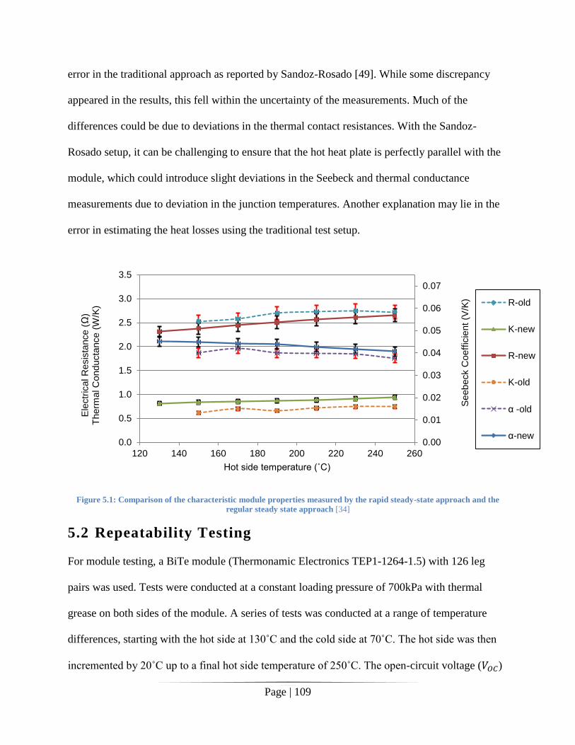
Page | 109

error in the traditional approach as reported by Sandoz-Rosado [49]. While some discrepancy

appeared in the results, this fell within the uncertainty of the measurements. Much of the

differences could be due to deviations in the thermal contact resistances. With the Sandoz-

Rosado setup, it can be challenging to ensure that the hot heat plate is perfectly parallel with the

module, which could introduce slight deviations in the Seebeck and thermal conductance

measurements due to deviation in the junction temperatures. Another explanation may lie in the

error in estimating the heat losses using the traditional test setup.

Figure 5.1: Comparison of the characteristic module properties measured by the rapid steady-state approach and the

regular steady state approach [34]

5.2 Repeatability Testing

For module testing, a BiTe module (Thermonamic Electronics TEP1-1264-1.5) with 126 leg

pairs was used. Tests were conducted at a constant loading pressure of 700kPa with thermal

grease on both sides of the module. A series of tests was conducted at a range of temperature

differences, starting with the hot side at 130˚C and the cold side at 70˚C. The hot side was then

incremented by 20˚C up to a final hot side temperature of 250˚C. The open-circuit voltage ( )

0.00

0.01

0.02

0.03

0.04

0.05

0.06

0.07

0.0

0.5

1.0

1.5

2.0

2.5

3.0

3.5

120 140 160 180 200 220 240 260

Seebeck C

oeff

icie

nt

(V/K

)

Ele

ctr

ical R

esis

tance (

Ω)

Therm

al C

onducta

nce (

W/K

)

Hot side temperature (˚C)

R-old

K-new

R-new

K-old

α -old

α-new

Page | 110

was recorded when the module reached a steady state at the set temperature. The current-voltage

sweep was then applied across the module, and the resulting load voltages were measured.

Figure 5.2 is a plot of the power versus the voltage to an open-circuit voltage ratio. The

maximum power occurred at approximately half the value of , which corresponds to the

predictions of the thermoelectric model used. Figure 5.3 shows the current and voltage values

measured at each point.

Figure 5.2: Comparison of power output vs. load voltage for different temperature differences

The repeatability tests were carried out on the same module at different days. Between each test,

the module was unloaded, cleaned, and loaded again. Cleaning is required to remove any

remnants of thermal grease used in the previous experiment. Thermal grease was applied on both

sides of the module at the start of every test to reduce any contact resistance between the

surfaces.

The tests were repeated on the same module over the entire temperature range multiple times.

The standard deviation was calculated at each temperature difference tested and then averaged

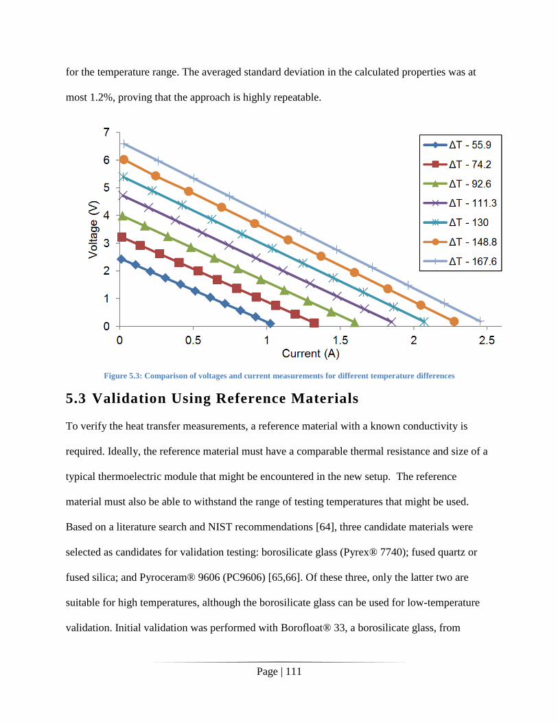
Page | 111

for the temperature range. The averaged standard deviation in the calculated properties was at

most 1.2%, proving that the approach is highly repeatable.

Figure 5.3: Comparison of voltages and current measurements for different temperature differences

5.3 Validation Using Reference Materials

To verify the heat transfer measurements, a reference material with a known conductivity is

required. Ideally, the reference material must have a comparable thermal resistance and size of a

typical thermoelectric module that might be encountered in the new setup. The reference

material must also be able to withstand the range of testing temperatures that might be used.

Based on a literature search and NIST recommendations [64], three candidate materials were

selected as candidates for validation testing: borosilicate glass (Pyrex® 7740); fused quartz or

fused silica; and Pyroceram® 9606 (PC9606) [65,66]. Of these three, only the latter two are

suitable for high temperatures, although the borosilicate glass can be used for low-temperature

validation. Initial validation was performed with Borofloat® 33, a borosilicate glass, from

Page | 112

SCHOTT North America Inc., because samples were available from the validation of an earlier

test stand [34]. Thermal conductivity from the manufacturer was used as a comparison. Fused

quartz was selected for future high-temperature validation due to the high cost of Pyroceram®

9606. Manufacturer data from Heraeus Quarzglas GmbH agrees well with published data by

Seeman [67] from 500 to 1000K, departing from the data published by Abdulgatov [68] at lower

temperatures. Due to this discrepancy among published values, the uncertainty in published

values is assumed to be +/–10%.

The Borofloat sample was tested for a range of mean temperatures from 100–160˚C. The tests

were conducted by keeping the cold side temperature constant at 70°C and incrementing the hot

side temperature by 20°C from 130–250°C. For each temperature difference, the temperature and

power measurements were taken after the sample reached a steady state.

The hot side and cold side temperatures were measured using Type K thermocouples inserted

just below the surface of the heater blocks. The heat rate was calculated by measuring the heater

input power averaged over ten minutes. By keeping a constant load pressure of 700kPa on the

sample, all effects due to contact resistance were assumed to be constant for all temperature

differences.

Thermal grease was used on both sides of the sample to reduce contact resistance. The test was

conducted by applying a fixed temperature difference across the sample, and measuring the heat

rate transferred through the sample. Using error analysis on measurements used in calculating the

conductivity resulted in an uncertainty of 5%. The results from the experiment were compared to

the values available in literature and are found to be in good agreement, as seen in Fig. 5.4. For

high-temperature validation, a quartz sample was tested over the entire range of test stand

Page | 113

operating temperatures.

Figure 5.4: Comparison of measured conductivity of borofloat and reference values

High-temperature validation was performed with fused quartz from GM Associates, Inc.

Thermal conductivity from the manufacturer was used as a comparison.

The quartz sample was tested for a range of mean temperatures from 125–435°C. The tests were

conducted by changing both the hot side and cold side temperatures to ramp the mean

temperature. The maximum hot side temperature reached was 650°C, which caused the hot side

blocks to start oxidizing. To observe the effect of oxidization on the conductivity results, tests

were also carried out as the average temperature was reduced. For each temperature difference,

the temperature and power measurements were taken after the sample reached a steady state.

0.00

0.20

0.40

0.60

0.80

1.00

1.20

1.40

1.60

90 100 110 120 130 140 150 160 170

Co

nd

uct

ivit

y (W

/m·K

)

Tmean (°C)

Conductivity Results for Borofloat

Theoretical Experimental

Linear (Theoretical) Linear (Experimental)

Page | 114

The pressure was kept constant at 700kPa, and power and temperature measurements were taken

in the same way as those with the Borofloat. No thermal grease was used, as the grease was rated

only up to 300°C. In the future, grafoil sheets should be used to reduce the effect of contact

resistance for high-temperature testing.

Using error analysis on the measurements used in calculating the conductivity resulted in an

uncertainty of 10%. The increase in uncertainty was mainly due to not accounting for the effect

of contact resistance. The results from the experiment were compared to the values available in

literature and are found to be in general agreement, as seen in Fig. 5.5.

Figure 5.5: Comparison of measured conductivity of quartz glass and reference values

Effects of oxidization on the results are also clear, as the error starts increasing at higher

temperatures. These errors continue even as the temperature is reduced. The maximum deviation

was observed when the tests were carried out as the heater cooling down from the maximum

0.00

0.50

1.00

1.50

2.00

2.50

90 140 190 240 290 340 390 440 490

Co

nd

uct

ivit

y (W

/m·K

)

T_mean (°C)

Conductivity Results for Quartz

Theoretical Experimental

Linear (Theoretical) Linear (Experimental)

Page | 115

temperature. This confirms that the copper had oxidized, and the module was cleaned to remove

any oxidized layers.

In conclusion, for quartz the conductivity results were found to be in good agreement up to

400°C, beyond which the copper heater blocks started oxidizing. The effect of oxidization was

also observed on cooling, causing large deviations from the theoretical values.

5.4 Uncertainty Analysis

Uncertainty is a non-negative parameter characterizing the dispersion of the values attributed to a

measured quantity. In practical testing, no measurement, however carefully made, can be

completely free of uncertainties. To reduce errors in measurement, the ability to measure and

minimize these uncertainties is extremely important.

The focus of this section is to accurately quantify the uncertainty in measuring the module

parameters based on the uncertainties of its constituent measurements. After knowing the

uncertainty values, steps can be taken to reduce overall uncertainty in the system. The

uncertainty analysis also helps accurately compare two results and differentiate between noise

and actual errors.

Measurement uncertainties are classified into two types by the National Institute of Standards

and Technology [69]:

Type A: These include uncertainties due to statistical analysis of data, such as finding the

standard deviation of a series of measurements. Type A errors, also known as random

errors, can be minimized by increasing the number of measurements.

Page | 116

Type B: These include uncertainties due to all other factors apart from the measured data,

such as calibration data or manufacturer’s data. Type B errors, also known as systematic

errors, are independent of the number of measurements but can be minimized by

calibration of instruments.

To calculate the uncertainty due to random errors, the standard deviation of the mean of the

measured set of values is calculated. In its simplest form, the standard deviation of the mean

denoted by ( ) for readings can be given as

√ √

∑

(5.1)

where is the average value for all terms ( ) given by ∑

(5.2)

The uncertainty due to standard deviation ( ) can be expressed in percentage as

(5.3)

To calculate uncertainty due to systematic errors, the values of standard deviation are obtained

directly from the manufacturer or vendor. These are normally given as an absolute error ( )

or a percent error ( . The uncertainty can then be calculated by Eqn. (5.3).

The total uncertainty from both Type A and type B components, known as standard uncertainty,

can be calculated by the root sum square method as

√ (5.4)

The standard uncertainty calculated in Eqn. (5.4) is calculated at one standard deviation.

Assuming that all the readings are normally distributed, this would mean that only 68% of

Page | 117

measurements would lie between ( ). To improve the confidence in measurements, the

uncertainty can be calculated at ( ) or even ( ), which would cover 95% or 99% of

measurements. To account for this, the standard uncertainty is multiplied by a coverage factor

( ). To avoid confusion with thermal conductance, the coverage factor will be noted as ( *).

In the rapid steady-state approach there are four quantities that are measured: the Seebeck

coefficient ( ), electrical resistance ( ), the thermal conductance ( ), and figure of merit ( ).

These are given as

(5.5)

(5.6)

(5.7)

(5.8)

The current measurement in Eqn. (5.6) is actually calculated using the voltage reading across a

shunt resistor .In Eqn. (5.7), the heat rate can be measured as the average product of voltage and

current over some time period. Thus, it is observed that in all four parameters, the main

measurements are those of temperature and voltage. The focus of this section is on the study of

uncertainty measurements of these two measurements, and their effect on the uncertainty of the

module parameters.

Voltage measurement

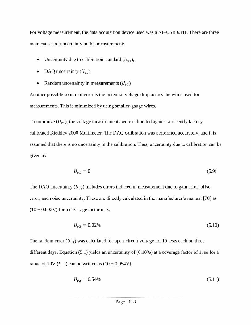
Page | 118

For voltage measurement, the data acquisition device used was a NI–USB 6341. There are three

main causes of uncertainty in this measurement:

Uncertainty due to calibration standard ( ),

DAQ uncertainty ( )

Random uncertainty in measurements ( )

Another possible source of error is the potential voltage drop across the wires used for

measurements. This is minimized by using smaller-gauge wires.

To minimize ( ), the voltage measurements were calibrated against a recently factory-

calibrated Kiethley 2000 Multimeter. The DAQ calibration was performed accurately, and it is

assumed that there is no uncertainty in the calibration. Thus, uncertainty due to calibration can be

given as

(5.9)

The DAQ uncertainty ( ) includes errors induced in measurement due to gain error, offset

error, and noise uncertainty. These are directly calculated in the manufacturer’s manual [70] as

(10 ± 0.002V) for a coverage factor of 3.

(5.10)

The random error ( ) was calculated for open-circuit voltage for 10 tests each on three

different days. Equation (5.1) yields an uncertainty of (0.18%) at a coverage factor of 1, so for a

range of 10V ( ) can be written as (10 ± 0.054V):

(5.11)

Page | 119

Using Eqns. (5.8), (5.9), and (5.10) the total uncertainty in voltage was calculated using Eqn.

(5.4), which came out to 0.15%:

(5.12)

Temperature measurement

For voltage measurement, the data acquisition device used was a NI–USB 9213. The report by

Nakos [71] for Sandia National Laboratories gives a detailed account of uncertainties observed

in thermocouple measurements. The main causes of uncertainty in this measurement are:

Thermocouple mounting error ( )

Type K thermocouple accuracy ( )

Thermocouple connector uncertainty ( )

Uncertainty due to the thermocouple extension cable ( )

Uncertainty due to the calibration standard ( )

DAQ uncertainty ( )

Random uncertainty in measurements ( )

Thermocouple mounting error ( ) is the error induced when the area to be measured is joined

to the thermocouple. Common mounting techniques include the use of thermal grease or

soldering, but due to the high test temperatures, both these techniques were incompatible in the

setup. Coupling in the setup was achieved by metal contact. The holes drilled for the

thermocouples were designed to have a transition fit to enable removal of thermocouples when

required and also to ensure good contact. Nakos [71] estimated this error as 0.75% or 2°C with

Page | 120

95% confidence, whichever is higher for all temperatures above 0°C. For an average temperature

of 650°C, the error is 0.75%.

(5.13)

The Type-K thermocouple is one of the most commonly used thermocouple types. The National

Institute of Standards and Technology estimated the uncertainty in measurement as 0.75% or

±2.2°C, whichever is higher [72]. For 150°C measurement, the error is 0.75%.

(5.14)

The uncertainty due to the connector arises when the material of the connector pins is not exactly

the same as the material of the thermocouple. An example of this would be an extension box

which works with multiple types of thermocouples. The system developed uses one such

extension panel. Nakos [71] estimated this error as ±0.5°C.

(5.15)

Uncertainty in the thermocouple cable has the same limitations as the thermocouple. The setup

developed uses a K-type extension cable.

(5.16)

To minimize ( ), the temperature measurements were calibrated using the setup described in

Section 4.6. After calibration, it was assumed

(5.17)

Page | 121

The DAQ uncertainty ( ) includes errors induced in measurement due to gain error, offset

error, and noise uncertainty. Using the values from the manufacturer’s manual [73], the overall

uncertainty was calculated using the formula in the manual as

√

(5.18)

The values provided in the manual were a gain error of 0.07%, an offset error of 6μV or 0.008%,

and noise of 200nV. All values were at full range (78.125mV). The error due to noise was

calculated using a coverage factor of 3 and using 10,000 measurements.

(5.19)

The random error ( ) was calculated for steady-state conditions for temperature readings at

20°C intervals from 130–250°C. It was found that the random error was the same, regardless of

the temperature. The sample size was 4,000 points for each test. Equation (5.1) yields an

uncertainty of (0.05%) at a coverage factor of 1, so for a range of 250°C, ( ) can be written as

(5.20)

Using Eqns. (5.12), (5.13), (5.14), (5.15), (5.16), (5.18), and (5.19) the total uncertainty in

voltage was calculated using Eqn. (5.4), which came out to

(5.21)

The uncertainty calculated was for all temperatures above 0°C using the information provided in

the NIST standard [72].

Uncertainty in module parameters

Page | 122

1. Seebeck coefficient ( )

The uncertainty analysis of Seebeck coefficient is quite straightforward:

√(

)

(

)

(

)

(5.22)

(5.23)

2. Electrical resistance ( )

In the rapid steady-state approach, the resistance is calculated using the slope of the voltage-

current line. To calculate the uncertainty in the slope is slightly complicated. In the test, the

module is loaded by stepping through different values of current. These values are assumed to

have negligible uncertainty. The line formed by all the points is in the general form

(5.24)

where is the voltage response, is the y-intercept ( ), is the current ,and is the slope of

the line and is the negative of the electrical resistance .

This is a three-step process. The first step is to calculate the best values of A and B using the co-

ordinates of points on the voltage-current line. These can be calculated as

∑

∑ ∑ ∑

(5.25)

∑ ∑ ∑

(5.26)

where ∑ ∑ (5.27)

Page | 123

Step two is to use these values to estimate the uncertainty in y and calculate uncertainty in x:

√

∑

(5.28)

√∑ (5.30)

where is the average value of when a test is repeated times. The uncertainty in is

calculated independent of the other points on the line.

The overall uncertainty can be calculated as

√

(5.31)

Finally, uncertainties in A and B can be calculated as

√∑

(5.32)

√

(5.33)

The random uncertainty in electrical resistance ( ) was thus calculated as

(5.34)

The electrical resistance is calculated as

(5.35)

The systematic uncertainty can be calculated as

Page | 124

√(

)

(

)

(

)

(

)

(5.36)

Where

(5.37)

(5.38)

Where with 1% uncertainty

Thus uncertainty in and can be expressed as

√(

)

(

)

(5.39)

√(

)

(

)

(5.40)

The systematic uncertainty in electrical resistance ( ) was thus calculated as

(5.41)

The overall uncertainty in electrical resistance ( ) is calculated as

√

(5.46)

(5.40)

3. Thermal conductance ( )

Page | 125

The uncertainty in thermal conductance can be separated into two parts: the uncertainty due to

instrumentation, and the uncertainty due to heat loss. The power is calculated as the product

of current and voltage. The current is calculated using a 10mΩ shunt resistor with 1%

uncertainty. The power equation can be rewritten as

(5.42)

where is the voltage across the shunt resister used to measure power. Assuming that the

uncertainty in voltage is same,

√(

)

(

)

(

)

(

)

(

)

(5.43)

Using above calculated values,

(5.44)

From thermal analysis, it was observed that at 650°C, the main heater power loss is around 2%.

Assuming no other systematic errors,

(5.45)

Total uncertainty in thermal conductance can be calculated as

√

(5.46)

(5.40)

Page | 126

In all of the measurements, uncertainties caused due to environmental factors such as

temperature, pressure, and humidity were assumed to be negligible. Thus, all of the measured

parameters are within the acceptable range of uncertainties for the desired test stand

specifications.

In this chapter, the preliminary data was reported and the test stand was validated by measuring

the thermal conductivity of known reference materials. Uncertainty analysis was performed to

estimate the deviation in values to be expected. Except for the thermal conductance, the

preliminary data matches very well with the old setup based on the steady state approach. Similar

trends are observed and the values of properties are within the uncertainty limits.

Where the thermal conductance is concerned, the main variation is in the heat rate values. Part of

the reason may be because of the fundamental difference in its calculation. The steady state

approach uses a passive approach in calculating heat losses by accounting and measuring all the

heat losses whereas the “rapid” steady state uses active accounting, where a guard heater

arrangement is used to minimize losses. Other reasons that may have caused the variation is the

overestimation of the temperature difference in the old setup as well as incorrect calculation of

heat losses. Further investigation is required to find out the cause of variation.

To validate the heat rate measurements, a reference material with known thermal conductivity

was used. Borofloat was selected as the reference material for low temperatures (up to 250°C)

and Quartz was selected for high temperatures (up to 400°C). The temperature was limited due to

oxidation of copper. These results were found to match very well with the available literature.

Page | 127

Finally, uncertainty analysis was performed to estimate the standard deviation in the

measurements. The resultant values were found to be well within the limits mentioned in the

specifications.

Page | 128

Chapter 6. Conclusion

6.1 Summary of Results

The overall goal of the project was to design and develop a test stand to evaluate properties of

high-temperature thermoelectric modules up to 650°C. To achieve this goal, a new testing

approach was developed for quick and accurate characterization. Three preliminary setups were

also built, based on techniques available in the current literature, to compare issues observed in

testing. A novel guard heater arrangement was used to minimize heat losses. To determine the

size of the guard heater, a thermal model was developed The test setup was validated by

comparing module properties from existing steady state setup as well as measuring thermal

conductivity of a reference material. Uncertainty analysis on the measurements confirmed that

the setup uncertainty is well within the specifications obtained from industrial partners and

laboratories manufacturing modules to be tested.

Preliminary testing was essential to determine the viability of any testing approach at higher

temperature. Based on a thorough review of previous published works, three classification of

testing approaches are most commonly used; the steady state approach, the Harman approach

and the Gao Min approach. For testing a module, researchers favored the steady-state approach,

as it is preferable to test a module in actual working conditions. A similar conclusion was

obtained from some preliminary experiments, which were carried out at low temperatures. The

biggest issue in the steady-state testing was to quantify the exact amount of heat flowing through

the module to determine the module’s conductance. For high-temperature testing, it was

concluded that accurate heat rate measurement would require active accounting of losses.

Page | 129

Active accounting of heat losses usually involves a shielding heater or a radiation shield. The

shielding heater or guard heater arrangement consists of a smaller heater surrounded by a larger

heater, both of which are maintained at the same temperature. In the literature, the main heater

block was made thin so that losses through the sides can be neglected. To account for side losses,

the guard heater block designed surrounds the main block on all sides. As both blocks are at the

same temperature, there is no heat loss from the main to the guard, effectively ensuring 1-D

conduction. Consequently, an important issue in steady-state testing was overcome.

Steady-state testing involves a scan of voltages and currents while a module is loaded with

different electrical resistors. At each load point the module should reach a steady state to achieve

good results. There is some difficulty in determining whether the module has reached a steady

state, especially during the first step, which changes the load from open circuit to short circuit.

This also causes long testing times. The new approach developed, called a rapid steady state, is

based on the steady state and overcomes all of these issues. This novel approach is a new

method, not appearing in the literature.

This rapid steady-state approach uses the same principle as the steady state in calculating the

Seebeck coefficient and thermal conductance. The difference lies in measuring the electrical

characteristics of the module. In the new method proposed, the module is electrically loaded and

unloaded over a very short time span, which avoids the thermal response of the module due to

Peltier cooling. By testing with different durations of the load steps, it was observed that the

optimum step duration was 10ms. The results were compared and the setup was validated using a

known reference material.

Page | 130

Three steps were taken for the validation of the setup. First, the results were tested for

repeatability by taking 10 scans each day for three different days. The scans were found to be

extremely repeatable and the standard deviation in properties averaged over a temperature range

from 130°C to 250°C was 1.2% at most. The second step was to validate the heat rate

measurements by calculating the thermal conductivity of a known reference material. Borofloat

was selected as a reference material at low temperatures, and quartz at high temperatures. The

measured values from both tests were comparable to those found in the literature up to 400°C,

beyond which oxidization effects of copper increased the error in measurement. Finally, a

detailed uncertainty analysis in measuring the module parameters was conducted. The

uncertainties is in values were 1% for the Seebeck coefficient, 2% for electrical resistance, and

3% for thermal conductance.

6.2 Contributions to the Thermoelectric Field

Several contributions were made to the field of thermoelectrics metrology. First and foremost, a

new testing approach was developed for testing of thermoelectric modules, called the rapid

steady-state method. The new method requires only a short time for testing, overcoming the

major drawback of the traditional steady-state approach. It is highly repeatable and is especially

useful for long-term testing, as the operating conditions of the module are not disturbed. This

versatile method can be used in the testing of both modules and bulk materials.

Additionally, the test setup designed is one of the first to be able to accurately test modules at

650°C. In previously published literature there are several setups that can test for material

properties, but the main issue in developing a setup for modules is calculating thermal properties.

This issue was overcome by using a novel guard heater arrangement to account for heat losses,

Page | 131

and thus accurately calculate the thermal properties. Another innovation in the test stand is the

ability to change the heater size with respect to the module being tested. If the size were kept the

same, it would cause large uncertainties in the test stand as the size of the module was reduced.

Changing the heater size ensures that there are no losses from the heater even for small sizes of

modules.

Furthermore, the test stand can be used for testing using the steady-state approach, the Harman

approach, and the Gao Min approach just by making minor adjustments. This is another feature

unique to the test stand.

6.3 Suggested Improvements and Future work

Some future work is recommended to resolve the various issues that were observed in

developing the first generation of test stand. The most important issue was oxidizing of copper at

high temperatures. The stand was built as a first prototype for high temperature testing. To keep

material costs low and ease in fabrication, copper was selected as the heater material. With

proven oxidation tendencies, using the same material for testing at 650°C will induce large

uncertainties. This was also witnessed in module validation using quartz. Aluminum nitride was

selected as the best candidate for testing at the full range and should be used in a future version

of the test stand now that the copper based system has proven to be highly effective. The second

material change suggested would be the insulation material. The material currently selected

frequently flakes off if scraped during testing, requiring thorough inspection of the heater

surface. If neglected, this can be a cause of large contact resistance between the surfaces. The

replacement material selected is 99% pure fused Silica ceramic, which has an even lower thermal

conductivity.

Page | 132

To reduce the effect of oxidization of the heater material as well as the thermoelectric module, a

design for implementing an inert atmosphere was briefly discussed. Implementation of this

design is an important next step required before testing at high temperatures. Enclosing the test

stand in a closed box will lead to difficulties in the loading of module. Currently, a hand crank is

used to maintain the loading pressure. This has to be moved frequently to account for the

changes in pressure due to thermal expansion of the heater materials. A pneumatic loading

assembly with external mounted controls is suggested for this purpose. This will enable the test

stand to change the loading pressure while enclosed inside the inert gas chamber.

The results from the quartz validation are within accepted limits for temperatures up to 400°C.

On incorporating the new heater material and inert gas enclosure, it is recommended to validate

the setup using quartz for the full range of temperatures, up to 650°C.

For the guard heater arrangement, the preliminary thermal modeling estimated the heat losses at

650°C to be 2% of the heater power. This needs to be verified experimentally and can be done by

changing the temperature difference applied across the module by a small value ( ) and

observing the change in heater power. This will also help calculate the sensitivity of the setup.

An important component assumed to be negligible in testing is the contact resistance. The

current method used to reduce contact resistance is to apply thermal grease. A focused study is

required to calculate and minimize the contact resistance between surfaces at higher

temperatures, where thermal paste cannot be used.

Finally, the test stand possesses the ability to test modules using different approaches. This has

been mentioned briefly as one of the contributions to the field of thermoelectrics. The natural

progression of this project would be to test and compare module properties using all of the

Page | 133

methods found in literature. Such a study would help make this test stand a benchmark in module

characterization.

Page | 134

Chapter 7. REFERENCES

[1] Energy Information Administration, 2011, International Energy Outlook 2011.

[2] U.S Department of Energy, 2008, Waste Heat Recovery: Technology and Opportunities in

U.S. Industry.

[3] United States Census, 2010, Total Midyear Population for the World.

[4] Bechtel R., 2010, Multi-Mission Radioisotope Thermoelectric Generator, The National

Aeronautics and Space Administration, Cleveland.

[5] FerroTec, “Advantages of Thermoelectric Cooling” [Online]. Available:

http://www.ferrotec.com/Technology/Thermoelectric/Thermalref04.

[6] Gould C. a., Shammas N. Y. a., Grainger S., and Taylor I., 2011, “Thermoelectric cooling

of microelectronic circuits and waste heat electrical power generation in a desktop

personal computer,” Materials Science and Engineering: B, 176(4), pp. 316–325.

[7] Gupta M. P., Sayer M.-H., Mukhopadhyay S., and Kumar S., 2011, “Ultrathin

Thermoelectric Devices for On-Chip Peltier Cooling,” IEEE Transactions on

Components, Packaging and Manufacturing Technology, 1(9), pp. 1395–1405.

[8] Sieko, “Sieko World’s First” [Online]. Available:

http://www.seikowatches.com/heritage/worlds_first.html.

[9] Kim I., 2000, “BiSb2 TeSe3 - based thin film thermoelectric generators,” Materials

Letters, 43(May), pp. 221–224.

[10] Custom Thermoelectric, “History of Thermoelectrics” [Online]. Available:

http://www.customthermoelectric.com/History.html.

[11] Kanatzidis M., 2009, New Thermoelectric Materials, Argonne National Laboratory,

Lemont.

[12] Tritt T. M., 2001, “Thermoelectric Materials : Principles, Structure, Properties, and

Applications,” Encyclopedia of Materials: Science and Technology, T.N. K.H.J.

Buschow, Ph.D., University of Amsterdam, Van Der Waals-Zeeman Institute, C.U. Robert

Cahn, M. Flemings, B. Ilschner, E. Kramer, S. Mahajan, and P. Veyssiere, eds., Elsevier

Inc.

[13] Muto A., 2008, “Device Testing and Characterization of Thermoelectric Nano

Composites,” MS Thesis, Mechanical Engineering, Massachusetts Institute of

Technology.

Page | 135

[14] Angrist S. W., 1961, “The Direct conversion of heat to electricity by means of a Nernst

effect Thermoelectric Generator,” PhD Dissertation, Mechanical Engineering Department,

Ohio State University.

[15] Hsu C.-T., Huang G.-Y., Chu H.-S., Yu B., and Yao D.-J., 2011, “Experiments and

simulations on low-temperature waste heat harvesting system by thermoelectric power

generators,” Applied Energy, 88(4), pp. 1291–1297.

[16] Gou X., Xiao H., and Yang S., 2010, “Modeling, experimental study and optimization on

low-temperature waste heat thermoelectric generator system,” Applied Energy, 87(10),

pp. 3131–3136.

[17] Garimella S., 2012, “Low-grade waste heat recovery for simultaneous chilled and hot

water generation,” Applied Thermal Engineering, 42, pp. 191–198.

[18] Stijepovic M. Z., and Linke P., 2011, “Optimal waste heat recovery and reuse in industrial

zones,” Energy, 36(7), pp. 4019–4031.

[19] Niu X., Yu J., and Wang S., 2009, “Experimental study on low-temperature waste heat

thermoelectric generator,” Journal of Power Sources, 188(2), pp. 621–626.

[20] Chen G., Dresselhaus M. S., Dresselhaus G., Fleurial J.-P., and Caillat T., 2003, “Recent

developments in thermoelectric materials,” International Materials Reviews, 48(1), pp.

45–66.

[21] Minnich A. J., Dresselhaus M. S., Ren Z. F., and Chen G., 2009, “Bulk nanostructured

thermoelectric materials: current research and future prospects,” Energy & Environmental

Science, 2(5), p. 466.

[22] Ponnambalam V., Lindsey S., Hickman N. S., and Tritt T. M., 2006, “Sample probe to

measure resistivity and thermopower in the temperature range of 300–1000 K,” Review of

Scientific Instruments, 77(7), p. 73904.

[23] Nakama T., Burkov A. T., Heinrich A., Oyoshi T., and Yagasaki K., 1998, Experimental

set-up for thermopower and resistivity measurements at 100-1300 K, Ieee.

[24] Martin J., Tritt T., and Uher C., 2010, “High temperature Seebeck coefficient metrology,”

Journal of Applied Physics, 108(12), p. 121101.

[25] Harman T. C., 1958, “Special Techniques for Measurement of Thermoelectric Properties,”

Journal of Applied Physics, 29(9), pp. 1373–1374.

[26] Buist, Richard J., 1992, “A New Method for Testing Thermoelectric Materials and

Devices,” 11th International Conference on Thermoelectrics, Arlington, Texas, p. 15.

Page | 136

[27] Mitrani D., Tomé J. A., Salazar J., Turó A., García M. J., Chávez J. A., and The A., 2005,

“Methodology for Extracting Thermoelectric Module Parameters,” 54(4), pp. 1548–1552.

[28] Fujimoto S., Kaibe H., Sano S., and Kajitani T., 2006, “Development of Transient

Measurement Method for investigating Thermoelectric Properties in High Temperature

Region,” Japanese Journal of Applied Physics, 45(11), pp. 8805–8809.

[29] Lau P. G., “Convection correction factor determination for use with the transient test

method for thermoelectric modules,” Eighteenth International Conference on

Thermoelectrics. Proceedings, ICT’99 (Cat. No.99TH8407), pp. 252–255.

[30] Vazquez J., Palacios R., Sanz-Bobi M. a., and Arenas A., 2003, “Test bench for measuring

the electrical properties of commercial thermoelectric modules,” Proceedings ICT’03.

22nd International Conference on Thermoelectrics (IEEE Cat. No.03TH8726), pp. 589–

593.

[31] Tanji Y., Nakagawa Y., Kisara K., Yasuoka M., Moriya S., Kumagai T., Niino M., and

Sato R., “Electric and thermal contact resistances of the new type thermoelectric module

assembled by a screwing method,” Eighteenth International Conference on

Thermoelectrics. Proceedings, ICT’99 (Cat. No.99TH8407), (1 999), pp. 260–265.

[32] Hsu C.-T., Huang G.-Y., Chu H.-S., Yu B., and Yao D.-J., 2011, “An effective Seebeck

coefficient obtained by experimental results of a thermoelectric generator module,”

Applied Energy, 88(12), pp. 5173–5179.

[33] Anatychuk L. I., and Havrylyuk M. V., 2011, “Procedure and Equipment for Measuring

Parameters of Thermoelectric Generator Modules,” Journal of Electronic Materials, 40(5),

pp. 1292–1297.

[34] Sandoz-Rosado E., and Stevens R. J., 2009, “Experimental Characterization of

Thermoelectric Modules and Comparison with Theoretical Models for Power

Generation,” Journal of Electronic Materials, 38(7), pp. 1239–1244.

[35] Muto a, Kraemer D., Hao Q., Ren Z. F., and Chen G., 2009, “Thermoelectric properties

and efficiency measurements under large temperature differences.,” The Review of

scientific instruments, 80(9), p. 093901.

[36] Rauscher L., Kaibe H. T., Ishimabushi H., Sano S., Muller E. W., and Platzek D., 2003,

“New approach for highly accurate efficiency determination of thermoelectric generator

modules,” Proceedings ICT’03. 22nd International Conference on Thermoelectrics (IEEE

Cat. No.03TH8726), pp. 508–511.

[37] Rauscher L., Fujimoto S., Kaibe H. T., and Sano S., 2005, “Efficiency determination and

general characterization of thermoelectric generators using an absolute measurement of

the heat flow,” Measurement Science and Technology, 16(5), pp. 1054–1060.

Page | 137

[38] Takazawa H., Obara H., Okada Y., Kobayashi K., Onishi T., and Kajikawa T., 2006,

“Efficiency measurement of thermoelectric modules operating in the temperature

difference of up to 550K,” 2006 25th International Conference on Thermoelectrics, pp.

189–192.

[39] Min G., and Rowe D. M., 2001, “A novel principle allowing rapid and accurate

measurement of a dimensionless thermoelectric figure of merit,” Measurement Science

and Technology, 12(8), pp. 1261–1262.

[40] Min G., Rowe D. M., and Kontostavlakis K., 2004, “Thermoelectric figure-of-merit under

large temperature differences,” Journal of Physics D: Applied Physics, 37(8), pp. 1301–

1304.

[41] Min G., 2010, “ZT Measurements Under Large Temperature Differences,” Journal of

Electronic Materials, 39(9), pp. 1782–1785.

[42] Middleton A. E., and Scanlon W. W., 1953, “Measurement of the Thermoelectric Power

of Germanium at Temperatures above 78°K,” Physical Review, 92(2), pp. 219–226.

[43] Sharath Chandra L. S., Lakhani A., Jain D., Pandya S., Vishwakarma P. N., Gangrade M.,

and Ganesan V., 2008, “Simple and precise thermoelectric power measurement setup for

different environments.,” The Review of scientific instruments, 79(10), p. 103907.

[44] Paul B., 2011, “Simple apparatus for the multipurpose measurements of different

thermoelectric parameters,” Measurement.

[45] Ahiska R., and Ahiska K., 2010, “New method for investigation of parameters of real

thermoelectric modules,” Energy Conversion and Management, 51(2), pp. 338–345.

[46] Ciylan B., and Yilmaz S., 2007, “Design of a thermoelectric module test system using a

novel test method,” International Journal of Thermal Sciences, 46(7), pp. 717–725.

[47] Iwasaki H., Yokoyama S., Tsukui T., Koyano M., Hori H., and Sano S., 2003, “Evaluation

of the Figure of Merit of Thermoelectric Modules by Harman Method,” Japanese Journal

of Applied Physics, 42(Part 1, No. 6A), pp. 3707–3708.

[48] Iwanaga S., Toberer E. S., LaLonde A., and Snyder G. J., 2011, “A high temperature

apparatus for measurement of the Seebeck coefficient.,” The Review of Scientific

Instruments, 82(6), p. 063905.

[49] Sandoz-Rosado E. J., 2009, “Investigation and Development of Advanced Models of

Thermoelectric Generators for Power Generation Applications,” Rochester Institute of

Technology.

[50] Buist, Richard J., 1995, “Methodology for Testing Thermoelectric Materials and

Devices,” CRC Handbook of Thermoelectrics, pp. 189–209.

Page | 138

[51] Rowe D. M., 2006, Thermoelectric s Handbook: Macro to nano, CRC/Taylor & Francis.

[52] Taylor J. R., 1997, An Introduction to Error Analysis, University Science Books, Sasalito,

California.

[53] Ferrotec Coorporation, “Photoveel II and Photoveel II-S - Machinable Nitride Ceramics”

[Online]. Available: http://www.ferrotec.com/products/ceramics/machineable/nitride/.

[54] Slack G. A., 1987, “The Intrinsic Thermal Conductivity of AIN,” Journal of Physics and

Chemistry of Solids, 48(7), pp. 641–647.

[55] Edgar J. H., Gu Z., Taggart K., Chaudhuri J., Nyakiti L., Lee R. G., and Witt R., 2006,

“Oxidation of Aluminum Nitride for Defect Characterization,” Material Research Society

Meeting, 892, pp. 1–6.

[56] Zhu Y., Mimura K., and Isshiki M., 2002, “Oxidation Mechanism of Copper at 623-1073

K.,” Materials Transactions, 43(9), pp. 2173–2176.

[57] Haugsrud R., 2003, “On the high-temperature oxidation of nickel,” Corrosion Science,

45(1), pp. 211–235.

[58] Lavrenko V. A., and Alexeev A. F., 1986, “High-temperature oxidation of boron nitride,”

Ceramics International, 12(1), pp. 25–31.

[59] Miller, Warren J., 1972, “High Temperature oxidation of Silicon Carbide,” Air Force

Institute of echnology.

[60] Gulbransen E. A., Andrew K. F., and Brassart F. A., 1963, “Oxidation of Molybdenum

550°C to 1700°C,” Journal of the Electrochemical Society, 110(9), pp. 952–959.

[61] Guha A., 1982, “Properties of CuBe C17510 for High Conductivity Applications,”

Stillwater, Oklahoma.

[62] Park J.-H., and Natesan K., 1993, “Oxidation of copper and electronic transport in copper

oxides,” Oxidation of Metals, 39(5-6), pp. 411–435.

[63] Kiethley, 2002, Model 2000 DMM.

[64] Flynn D. ., 2013, “Thermophysics consultant, National Institute of Standards and

Technology, USA.”, Private Communication

[65] Müller E., Stiewe C., Rowe D., and Williams S., 2006, “Precision Thermal Conductivity

Measurements of materials,” Thermoelectrics Handbook Macro to Nano, pp. 26–8 – 26–9.

Page | 139

[66] Buzovkina T., and Men’ A., 1972, “Use of fused quartz as a reference standard in

comparative methods of thermal conductivity measurements,” Journal of Engineering

Physics.

[67] Seemann H. E., 1928, “The Thermal and Electrical Conductivity of Fused Quartz as a

Function of Temperature,” Physical Review, 31(1), pp. 119–129.

[68] Abdulagatov I. M., Emirov S. N., Tsomaeva T. A., Gairbekov K. . A., Askerov S. Y. Y.,

and Magomedova N. A., 2000, “Thermal conductivity of fused quartz and quartz ceramic

at high temperatures and high pressures,” Journal of Physics and Chemistry of Solids,

61(5), pp. 779–787.

[69] Taylor B. N., and Kuyatt C. E., 1994, Guidelines for Evaluating and Expressing the

Uncertainty of NIST Measurement Results, Physics Laboratory, National Institute of

Standards and Technology, Gaithersburg, MD.

[70] National Instruments, 2013, NI 6341/6343 Specifications.

[71] Nakos J. T., 2004, Uncertainty Analysis of Thermocouple Measurements Used in Normal

and Abnormal Thermal Environment Experiments at Sandia’s Radiant Heat Facility and

Lurance Canyon Burn Site, Sandia National Laboratories, Albuquerque, New Mexico.

[72] Nationa Institute of Standards and Technology, 2011, Type K thermocouple reference

Table, N.I.S.T.

[73] National Instruments, 2013, NI USB 9213 Manual, National Instruments.

Page | 140

Appendix A

Test Procedure:

The test begins by cleaning the thermal grease on the module from the previous test as well as

cleaning the surfaces of the heaters. On a clean module, a new layer of thermal grease is applied.

The module is placed on the main heater block and the cold side assembly is lowered with the

help of a lead screw. When the system will be placed in an inert environment, the lowering will

be performed with the help of a pneumatic cylinder. The lead screw rests on top of a load cell

which measures the applied pressure. Two pieces of insulation are then slid into position to

reduce heat loss.

Once optimal loading pressure is reached, the chiller is turned on. This controls the temperature

of the cold plate and removes heat dumped by the system. Using the VI created in LABVIEW,

the temperatures for main heater block, guard heater block and the cold side heater block are set.

The temperatures for the main and cold heater blocks are set as values in Celsius, whereas the

guard heater block temperature is set as a difference with respect to the main heater temperature.

The entire setup takes about 30 minutes to reach steady state. Once the system reaches the set

temperatures, a scan is performed and the data is recorded and exported to Excel. Post processing

converts this data into required parameters.

Page | 141

Appendix B

Page | 142

Page | 143

Page | 144

Page | 145

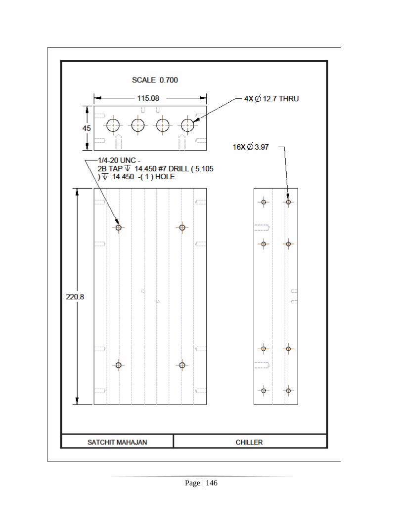
Page | 146

Documents

A Test setup for characterizing high-temperature