Tellus (2006), 58B, 463–475 C© 2006 The AuthorsJournal compilation C© 2006 Blackwell Munksgaard

Printed in Singapore. All rights reservedT E L L U S

A test of sensitivity to convective transport in a globalatmospheric CO2 simulation

By H. BIAN 1∗, S . R . KAWA 2, M. CHIN 2, S . PAWSON 2, Z . ZHU 2, P. RASCH 3 and S . WU 4,1UMBC Goddard Earth Science and Technology Center, NASA Goddard Space Flight Center, Greenbelt, MD 20771,USA; 2NASA Goddard Space Flight Center, Greenbelt, MD 20771, USA; 3National Center for Atmospheric Research,

Boulder, CO 80307, USA; 4Harvard University, Cambridge, MA 02138, USA

(Manuscript received 9 January 2006; in final form 3 July 2006)

ABSTRACT

Two approximations to convective transport have been implemented in an offline chemistry transport model (CTM) to

explore the impact on calculated atmospheric CO2 distributions. Global CO2 in the year 2000 is simulated using the CTM

driven by assimilated meteorological fields from the NASA’s Goddard Earth Observation System Data Assimilation

System, Version 4 (GEOS-4). The model simulates atmospheric CO2 by adopting the same CO2 emission inventory and

dynamical modules as described in Kawa et al. (convective transport scheme denoted as Conv1). Conv1 approximates

the convective transport by using the bulk convective mass fluxes to redistribute trace gases. The alternate approximation,

Conv2, partitions fluxes into updraft and downdraft, as well as into entrainment and detrainment, and has potential to

yield a more realistic simulation of vertical redistribution through deep convection. Replacing Conv1 by Conv2 results

in an overestimate of CO2 over biospheric sink regions. The largest discrepancies result in a CO2 difference of about

7.8 ppm in the July NH boreal forest, which is about 30% of the CO2 seasonality for that area. These differences are

compared to those produced by emission scenario variations constrained by the framework of Intergovernmental Panel

on Climate Change (IPCC) to account for possible land use change and residual terrestrial CO2 sink. It is shown that

the overestimated CO2 driven by Conv2 can be offset by introducing these supplemental emissions.

1. Introduction

The importance of characterizing transport error in forward mod-

els has been widely recognized, and substantial effort has been

devoted to quantifying such error (e.g. Denning et al., 1999;

Engelen et al., 2002; Palmer et al., 2003). Tropospheric con-

stituent transport occurs by advective, diffusive and convective

processes and inadequacies in any of these mechanisms will lead

to error in simulated trace gas concentrations. The primary goal

of this study is to explore the extent to which the treatment of

convective transport impacts the atmospheric CO2 distribution.

The study uses a chemistry transport model (CTM) with speci-

fied surface flux distributions and perturbs the representation of

convective transport in this system, while all other processes are

held fixed. The two approximations to convective transport are

referred to as Conv1 and Conv2. Following Kawa et al. (2004),

Conv1 uses a constraint of the total convective mass flux (CMF),

in which air parcels entrained at cloud base are transported up-

wards, detraining at a rate proportional to the convergence of

∗Corresponding author.

e-mail: Bian@code916.gsfc.nasa.gov

DOI: 10.1111/j.1600-0889.2006.00212.x

CMF. Conv2 is a potentially more accurate approximation, us-

ing information on updraft and downdraft, as well as entrainment

and detrainment rates; this allows for air parcels to be ventilated

within the entire cloud ensemble and also to enter or leave the

cloud environment at any altitude, subject to the same constraints

on total CMF. All fields used were archived as 3 h averages from

the Goddard Earth Observation System Version 4 (GEOS-4) data

assimilation system (Bloom et al., 2005). Hence, the two algo-

rithms represent cloud convective transport from a very simple

to a relatively complex form. The uncertainty induced by them

will represent one term in the potential cloud convection error.

We will further identify regions where mixing ratios are sensitive

to atmospheric convection, with an overall goal to assist regional

carbon cycle simulation. This study complements a number of

other approaches to quantifying transport uncertainty, in at least

two ways.

First, several studies have attempted to quantify the differ-

ences between atmospheric transport using different algorithms

of atmospheric convection. Mahowald et al. (1995) used a col-

umn model to quantify transport differences among seven dif-

ferent cumulus convection parameterizations, illustrating vastly

different results that are sensitive to aspects of ‘closure’ (the cri-

teria used to determine onset of convection, dependent on some

Tellus 58B (2006), 5 463

464 H. BIAN ET AL.

aspect of horizontal mass convergence below cloud base) and

to the cloud assumptions used in the convection module itself.

Gilliland and Hartley (1998) demonstrated, using two versions of

a GCM in which the CMF differs substantially, that the strength

of convective transport has a discernable impact on interhemi-

spheric exchange of long-lived trace gases. Olivie et al. (2004)

also found significantly different radon distributions in the upper

troposphere and lower stratosphere in their simulations with con-

vective mass fluxes from two different resources [one archived

from the European Center for Medium-Range Weather Fore-

casts (ECMWF) and another from off-line diagnoses calculated

with a parameterization that mimics the ECMWF-scheme using

archived winds, pressures, temperatures, specific humidities and

evaporation rates]. The present study differs from these previous

works in that here the GEOS-4 convection scheme to produce the

cloud field is not changed, but the manner in which the archived

CMF fields are used in the CTM does change.

Second, a number of studies have examined transport of

trace gases using different meteorological fields and/or different

CTMs. At the forefront of such comparison is the Atmospheric

Tracer Transport Model Intercomparison Project (TransCom),

which was created to quantify and diagnose the uncertainty in

inverse calculations of the global carbon budget that resulted

from errors in simulated atmospheric transport (Law et al., 1996,

Denning et al., 1999, Gurney et al., 2003). These multimodel as-

sessments indicate that the model behaviour differs substantially;

however, it is difficult to diagnose the determining factors that

cause these difference since the participating models are differ-

ent not only in convective parameterization but also in spatial

resolution, advection schemes and most importantly, meteoro-

logical fields (Gurney et al., 2003). Our approach presented here

allows testing of the convection uncertainty within a single model

framework and driven by the same meteorological fields, there-

fore eliminating all compounding perturbing factors other than

the model convective transport methodology. The information

of where, when, and how large are CO2 uncertainties induced

by different convection schemes will also be useful to interpret

inverse studies using our CTM. Note that this approach does not

address the most fundamental issues related to the ability of the

parent general circulation model to correctly capture the location

and strength of convection events but focuses on the application

of CMF for long-lived trace gas transport.

An additional goal of this study is to examine the sensitivity

of atmospheric CO2 to its regional source/sink uncertainty. The

study of model convection transport raises a question: which

cloud convective scheme is more appropriate to manifest atmo-

spheric vertical transport in the context of model-measurement

agreement? The answer is not simple, since the simulation capa-

bility also depends on constraint of the CO2 source/sink. Global

decadal budgets summarized for the 1980s and 1990s infer a

large residual terrestrial sink for atmospheric CO2 with attached

uncertainty of 50–100% or more (IPCC, 2001). This so-called

‘missing sink’ for CO2 epitomizes a major uncertainty in the

current understanding of carbon cycle processes. In this study,

in addition to a ‘standard’ emission scenario (Emi1) proposed

by TransCom3, we construct two residual terrestrial CO2 fluxes

(with the total emissions referred as Emi2 and Emi3) that are

constrained within the IPCC, 2001 CO2 to address the following

questions: (1) How sensitive is atmospheric CO2 change in re-

sponse to its regional source/sink change? (2) Is the variation of

atmospheric CO2 inferred from surface flux uncertainty compa-

rable to the variation induced from changing convective transport

representations?

This paper starts with a description of the model frame-

work in Section 2, in particular the two convection approxima-

tions. The observational data and the potential errors in model-

observational comparisons due to different spatial and temporal

resolutions in data are also explained in Section 2. Section 3

presents the CO2 simulation uncertainties in a single forward

model framework that are induced by two different convection

approaches and by three emission scenarios. Conclusions and

implications of this work are given in Section 4.

2. Description of model and data

2.1. Model framework

An offline CTM framework has been designed in such a way

that each physical and chemistry module can be upgraded eas-

ily through an interface. The goal of developing such an offline

CTM is to assess the impacts on tracer distributions due to the

different dynamical and chemical approaches. For this study, the

advection algorithm adopts the code of Lin and Rood (1996),

which is formulated in flux form and employs a semi-Lagrangian

algorithm. This advection algorithm has been extensively eval-

uated in tropospheric and stratospheric CTMs (Lin and Rood,

1996; Bey et al., 2001; Chin et al., 2002; Douglass et al., 2003)

and implemented in several global chemistry and transport mod-

els including a trace gas transport model (PCTM) (Kawa et al.,

2004) and the Goddard Chemistry Aerosol Radiation and Trans-

port (GOCART) model (Chin et al. 2002, 2004). Boundary layer

turbulence and atmospheric diffusion is calculated from the dif-

fusion equation, same as in GOCART and PCTM. Since our

study focuses on the representation of convective transport in a

CTM, we will describe in detail the two cloud convection ap-

proximations in Section 2.2. The model, in this study, is driven

by time-averaged analysed meteorological fields from NASA’s

GEOS-4 assimilation system (Bloom et al., 2005).

A ‘standard’ emission scenario (denoted as Emi1) based on

the compilations of TransCom 3 (Gurney et al., 2002) is used

in our convection transport uncertainty study. Emi1 comprises a

fossil fuel combustion with a global total of 6.17 Pg C yr−1 in

1995 (Andres et al., 1996), a seasonally balanced terrestrial bio-

sphere based on computations of net primary productivity from

the Carnegie–Ames–Stanford Approach (CASA) (Randerson

et al., 1997), and an air–sea gas exchange (−2.2 Pg C yr−1) from

Tellus 58B (2006), 5

TEST OF SENSITIVITY TO CONVECTIVE TRANSPORT 465

1◦ × 1◦ monthly mean CO2 fluxes derived from sea-surface

pCO2 measurements (Takahashi et al., 2002). CO2 source ox-

idized from the reduced carbon trace gases (CO, CH4, and

NMVOCs) is accounted simply as part of the fossil fuel emission

at the surface. While the fossil fuel emission is given as annual

mean rates, the fluxes from biosphere and ocean are provided as

monthly means which are compiled from the diurnal averages.

All sources/sinks are dealt in the surface layer of the model. The

potential errors in reproducing atmospheric CO2 due to using

monthly mean fluxes had been discussed in Kawa et al. (2004);

the diurnal cycle of biospheric CO2 is weakened in the planetary

boundary layer (PBL) in source/sink regions. Suntharalingam et

al. (2005) reported the potential errors of simulated CO2 due

to releasing reduced carbon at surface. We will address this in

Section 3.1.1 when comparing simulated surface CO2 with ob-

servations.

2.2. Representation of convective transport

A suite of meteorological and physical fields is archived from

GEOS-4. For transport studies, Bloom et al. (2005) describe the

utility of time-averaged meteorological data (winds and tempera-

tures) along with tendencies from the physical parameterizations

in the underlying GCM. Convection in GEOS-4 is represented

by two models: deep convection follows Zhang and McFarlane

(1995) while shallow convection is based on Hack et al. (1994).

The parameterization of deep convection in GEOS-4 introduced

the concepts of updraft and downdraft, as well as the entrainment

and detrainment associated with the updraft and downdraft, to

describe penetrative cumulus convection (Zhang and McFarlane,

1995). Moist upward convection is initiated when there is con-

vective available potential energy (CAPE) for reversible ascent

of an undiluted parcel from the subcloud layer. Each updraft is

represented as an entraining plume with a characteristic frac-

tional entrainment rate. Detrainment associated with updraft is

confined to a thin layer near the plume top where the mass car-

ried upward is expelled into the environment. Downdrafts are

assumed to exist when there is precipitation production in the

updraft ensemble. The downdrafts start at or below the bottom

of the updraft detrainment layer and penetrates down to the sub-

Table 1. The summarization of main features and differences in two convection schemes

Conv1 Conv2

References Kawa et al. (2004) Collins et al. (2004)

Implemented in PCTM MATCH; GEOS-CHEM

Differentiate tracer in & out cloud No Yes

Numerical scheme Semi-implicit Upstream differencing

Differentiate shallow and deep cloud in CTM No Yes

Constrained by Cloud mass flux Shallow: shallow cloud mass flux; overshoot parameter

Deep: updraft; downdraft; updraft entrainment; updraft detrainment;

downdraft entrainment

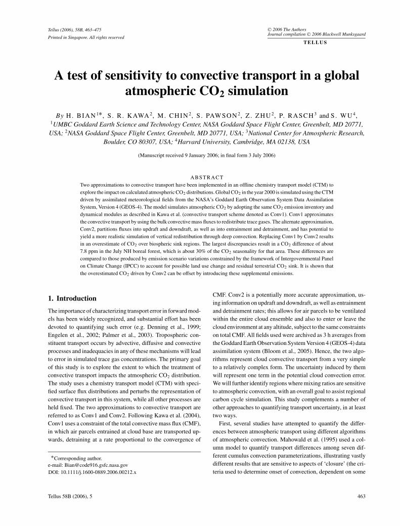
Fig. 1. Schematics of the cloud mass fluxes for Conv1 (C: total cloud

mass flux; S: compensating large-scale subsidence) and Conv2 (U:

updraft; UE: updraft entrainment; UD: updraft detrainment; AD:

environment subsidence to compensate in-cloud updraft; D: downdraft;

DE: downdraft entrainment; AU: environment upward to compensate

in-cloud downdraft). The shallow cloud model for Conv2 (not shown in

figure) is similar to Conv1.

cloud layer. A complete set of CMF data is archived from the

shallow and deep convection modules, as described below.

Table 1 shows the main features and differences of the two

convective transport approaches tested in this study. These are

represented schematically in Fig. 1. The first cloud convection

scheme (Conv1) was implemented in PCTM and used to simu-

late atmospheric CO2 distribution (Kawa et al., 2004). This is a

semi-implicit convective module, constrained by the subgrid-

scale cloud mass flux from the assimilation system. Vertical

cloud transport in layer k is calculated by

qt+�tk − qt

k = g�t

�pk[Ck+1(qk+1 − qk)−Ck(qk −qk−1)]t+�t/2, (1)

where q is the tracer concentration, and Ck, Ck+1 are the net

convective mass fluxes (shallow and deep convection updraft

minus downdraft) at the upper and lower edges of a layer, t is

the model time step, and �pk/g is the air mass of a layer. The

term on the right-hand side of the equation calculates the tracer

mass change in layer k due to cloud fluxes and this tracer mass

change is taken at the middle of the time step (semi-implicit).

The second convective transport algorithm (Conv2) uses ad-

ditional output from the shallow (Hack et al., 1994) and deep

(Zhang and McFarlane, 1995) convection codes and is de-

signed to be consistent with the subgrid cloud parameterizations

Tellus 58B (2006), 5

466 H. BIAN ET AL.

developed in GCM. It has been implemented in several global

models (Eneroth et al., 2003a; Zender et al., 2003; Li et al., 2005;

Millet et al., 2005). Shallow convection uses cloud mass fluxes

and overshoot parameters from the Hack scheme to mix the pas-

sive constituents in layers k − 1 through k + 1 for the vertical

k layer. This transport is essentially the same as that done in

Conv1. The deep convection distinguishes the mass fluxes among

updraft, downdraft, updraft entrainment, updraft detrainment and

downdraft entrainment, and employs all of them to drive cloud

vertical mixing. It uses simple first order upstream biased finite

differences to solve the steady-state mass continuity equations

for the ‘bulk’ updraft and downdraft mixing ratios and the mass

continuity equation for the gridbox mean (Collins et al., 2004).

∂(Mxqx)

∂ p= Exqe − Dxqx (2)

∂ q

∂t= ∂

∂ p[Mu(qu − q) + Md(qd − q)] (3)

The subscript x is used to denote the updraft (u) or downdraft

(d) quantity. Here, Mx is the mass flux in units of Pa s−1 defined at

the layer interfaces, qx is the mixing ratio of the updraft or down-

draft. qe is the mixing ratio of the quantity in the environment

(that part of the grid volume not occupied by the up and down-

drafts), and is assumed to be the same as the gridbox averaged

mixing ratio q. Ex and Dx are the entrainment and detrainment

rates (units of s−1) for the up- and downdrafts. Updrafts are al-

lowed to entrain or detrain in any layer. Downdrafts are assumed

to only entrain and all of the mass is assumed to be deposited

into the surface layer. The tracer mass flux and mixing ratio are

integrated along the pressure p and time t, respectively.

Conv2 in our CTM takes full advantage of the underlying

GCM cloud parameterization to transport tracers. The algorithm

of Conv2 solves three variables: tracer-mixing ratios in cloud up-

draft, cloud downdraft, and environment by considering tracer

mass changes associated with these regimes (eqs. 2–3). The ob-

jective of Conv2 is to keep the tracer vertical transport in a pene-

trating cumulus as efficient as the energy and moisture transport

in its underlying GCM. For example, in a cloud updraft regime,

Conv2 sucks in environmental tracer into cloud through the up-

draft entrainment flux at the low part of the cloud and then trans-

ports the tracer upward inside the updraft regime with the updraft

flux. When the cloud reaches a level where updraft detrainment

appears, usually at the top part of a deep cloud, Conv2 begins to

return the tracer to the environment in the proportion to the cloud

updraft detrainment. In this way, Conv2 can efficiently transport

tracer vertically inside cloud updraft (and downdraft) and af-

fect environment tracer mixing ratio through cloud convergent

(entrainment) and divergent (detrainment) fluxes.

On the other hand, Conv1 uses only the total net cloud flux

to solve a layer’s mean mixing ratio by exchanging with ad-

jacent layers. There are two limitations in this approach: (1)

tracer transport cannot proceed unmixed through more than one

vertical gridcell per time step in a penetrative cumulus; (2) the

fluxes in opposite directions (updraft versus downdraft) are can-

celled out by an equivalent amount in the total cloud mass flux.

This will decrease convective mixing relative to treating up and

down drafts separately, although the downdraft component is

generally small (see below). Note that the reality of transport by

either method depends on the reality of subgrid-scale physical

parameterization in the parent GCM, which is highly uncertain

and representative only in a statistical sense in current models

(Mahowald et al., 1995).

2.3. Observational data

The observational data of atmospheric CO2 mixing ratio used to

evaluate model simulation are obtained from NOAA Climate

Monitoring and Diagnostics Laboratory (CMDL) Carbon Cycle

Greenhouse Gases (CCGG) (http://www.cmdl.noaa.gov/ccgg/

index.html). Samples are taken at NOAA CMDL Carbon Cy-

cle Cooperative Global Air Sampling Network sites. They are

measured by a non-dispersive infrared absorption technique in

air samples collected in glass flasks. Samples are collected in

pairs approximately once a week at local noon for 41 surface

(non-baseline) fixed sites and aircraft measurement over 14 sites

are made usually one to two times per month in local afternoon.

The pair difference is calculated, and samples with a pair differ-

ence greater than 0.5 ppm are flagged. Flagged data are excluded

from our comparisons.

There are spatial and temporal resolution differences between

observational and simulated data. The model results are daily

or monthly averages at 2 latitude × 2.5 longitude spatial reso-

lution, while observational data are ‘instantaneous’ taken sev-

eral times per month at specific site locations. Spatial mismatch

of simulation (grid mean value) and measurement (site loca-

tion) leads to ‘representation error’ and temporal covariance be-

tween mixed-layer height and biosphere-atmosphere exchange

fluxes may cause biases, ‘rectification errors’, over diurnal or

seasonal timescales (Denning et al., 1996; Gerbig et al., 2003;

Yi et al., 2004). Furthermore, the ‘representation error’ is not

fixed because footprint (the surface area inside which the data

are correctly represented by the measurement at a site) varies

with height, wind direction, meteorological conditions (stabil-

ity) and the magnitude of the CO2 flux (Rannik et al., 2000;

Aubinet et al., 2001; Eneroth et al., 2003, Murayama et al.,

2004). An investigation of the footprint in a measuring site in

western Siberia indicated that it is only ten to 100 km in July but

much larger in winter (Eneroth et al., 2003b). The CO2 Budget

and Rectification Airborne (COBRA) study in August 2000 also

pointed out that models require horizontal resolution finer than

∼30 km to fully resolve spatial variations of atmospheric CO2

in the boundary layer over the continent (Gerbig et al., 2003).

Therefore, the inherent features in the simulation and model data

will result in the differences in model-observation comparisons

even for an ideal simulation, and the errors vary with time and

location.

Tellus 58B (2006), 5

TEST OF SENSITIVITY TO CONVECTIVE TRANSPORT 467

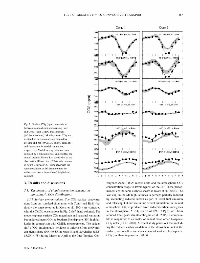
Fig. 2. Surface CO2 (ppm) comparisons

between standard simulation (using Emi1

and Conv1) and CMDL measurement

(left-hand column). Monthly mean CO2 and

its standard deviation are represented by

dot-line and bar for CMDL and by dash-line

and shade area for model simulation,

respectively. Model mixing ratio has been

adjusted by a constant offset value so that the

annual mean at Mauna Loa equals that of the

observation (Kawa et al., 2004). Also shown

in figure is surface CO2 simulated with the

same conditions as left-hand column but

with convection scheme Conv2 (right-hand

column).

3. Results and discussions

3.1. The impacts of cloud convection schemes onatmospheric CO2 distributions

3.1.1 Surface concentrations. The CO2 surface concentra-

tions from our standard simulation with Conv1 and Emi1 (ba-

sically the same setup as in Kawa et al., 2004) are compared

with the CMDL observations in Fig. 2 (left-hand column). The

model captures surface CO2 magnitude and seasonal variation,

but underestimates CO2 at Southern Hemisphere (SH) high lat-

itudes in comparison with CMDL measurements. The sudden

shift of CO2 mixing ratio is evident in influence from the North-

ern Hemisphere (NH) to SH in Mahe Island, Seychelles (SEY:

55.2N, 4.7S) during March to April as the Inter-Tropical Con-

vergence Zone (ITCZ) moves north and the atmospheric CO2

concentration drops to levels typical of the SH. These perfor-

mances are the same as those shown in Kawa et al. (2004). The

low CO2 in the SH high latitudes is perhaps partially induced

by accounting reduced carbon as part of fossil fuel emission

and releasing it at surface in our current simulation. In the real

atmosphere, CO2 is produced from reduced carbon trace gases

in the atmosphere. A CO2 source of 0.9–1.3 Pg C yr−1 from

reduced trace gases (Suntharalingam et al., 2005) is compara-

ble in magnitude to estimates of annual mean ocean biosphere

CO2 sinks (IPCC, 2001). A recent study points out that includ-

ing the reduced carbon oxidation in the atmosphere, not at the

surface, will result in an enhancement of southern hemispheric

CO2 (Suntharalingam et al., 2005).

Tellus 58B (2006), 5

468 H. BIAN ET AL.

In order to investigate the impacts of different convective

transport algorithms on atmospheric CO2 distributions, we run

the model with the Conv2 convective transport scheme described

in Section 2.2. Figure 2 shows the comparisons of model sim-

ulations from Conv1 and Conv2 with observations at selected

CMDL surface sites for their representativeness of major geo-

graphic locations and distinct features of carbon emission fluxes:

NH high latitude (ALT), NH mid-latitude land regions (MHD),

NH background (MLO), tropical regions (SEY), SH biomass

burning (ASC), and SH high latitude (PSA).

While Conv1 captures the observed seasonal variation of CO2

at station ALT, Conv2 shows a significant summer enhance-

ment, thus a reduced magnitude of such variation. For example,

the minimum CO2 mixing ratio in the summer is 362.2 ppm

in Conv1 but 366.0 in Conv2 at ALT; consequently, the CO2

seasonal amplitude is 14.5 ppm in Conv1 but only 11.0 ppm in

Conv2. A sharp decrease of CO2 mixing ratio from March to

April observed at station SEY is captured by Conv1, whereas

not by Conv2. This means that Conv2 does not represent the

tracer variation during the ITCZ transition. Both convective ap-

proximations underestimate CO2 during the first half of the year

at station ASC, however, the CO2 seasonality of Conv1 is closer

to that of observations.

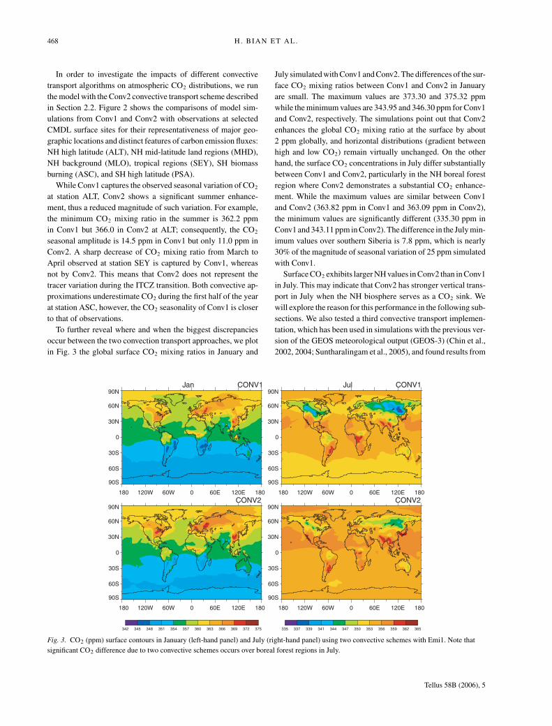
To further reveal where and when the biggest discrepancies

occur between the two convection transport approaches, we plot

in Fig. 3 the global surface CO2 mixing ratios in January and

Jan CONV1

180 120W 60W 0 60E 120E 180

90S

60S

30S

0

30N

60N

90N Jul CONV1

180 120W 60W 0 60E 120E 180

90S

60S

30S

0

30N

60N

90N

CONV2

180 120W 60W 0 60E 120E 180

90S

60S

30S

0

30N

60N

90N

342 345 348 351 354 357 360 363 366 369 372 375

CONV2

180 120W 60W 0 60E 120E 180

90S

60S

30S

0

30N

60N

90N

335 337 339 341 344 347 350 353 356 359 362 365

Fig. 3. CO2 (ppm) surface contours in January (left-hand panel) and July (right-hand panel) using two convective schemes with Emi1. Note that

significant CO2 difference due to two convective schemes occurs over boreal forest regions in July.

July simulated with Conv1 and Conv2. The differences of the sur-

face CO2 mixing ratios between Conv1 and Conv2 in January

are small. The maximum values are 373.30 and 375.32 ppm

while the minimum values are 343.95 and 346.30 ppm for Conv1

and Conv2, respectively. The simulations point out that Conv2

enhances the global CO2 mixing ratio at the surface by about

2 ppm globally, and horizontal distributions (gradient between

high and low CO2) remain virtually unchanged. On the other

hand, the surface CO2 concentrations in July differ substantially

between Conv1 and Conv2, particularly in the NH boreal forest

region where Conv2 demonstrates a substantial CO2 enhance-

ment. While the maximum values are similar between Conv1

and Conv2 (363.82 ppm in Conv1 and 363.09 ppm in Conv2),

the minimum values are significantly different (335.30 ppm in

Conv1 and 343.11 ppm in Conv2). The difference in the July min-

imum values over southern Siberia is 7.8 ppm, which is nearly

30% of the magnitude of seasonal variation of 25 ppm simulated

with Conv1.

Surface CO2 exhibits larger NH values in Conv2 than in Conv1

in July. This may indicate that Conv2 has stronger vertical trans-

port in July when the NH biosphere serves as a CO2 sink. We

will explore the reason for this performance in the following sub-

sections. We also tested a third convective transport implemen-

tation, which has been used in simulations with the previous ver-

sion of the GEOS meteorological output (GEOS-3) (Chin et al.,

2002, 2004; Suntharalingam et al., 2005), and found results from

Tellus 58B (2006), 5

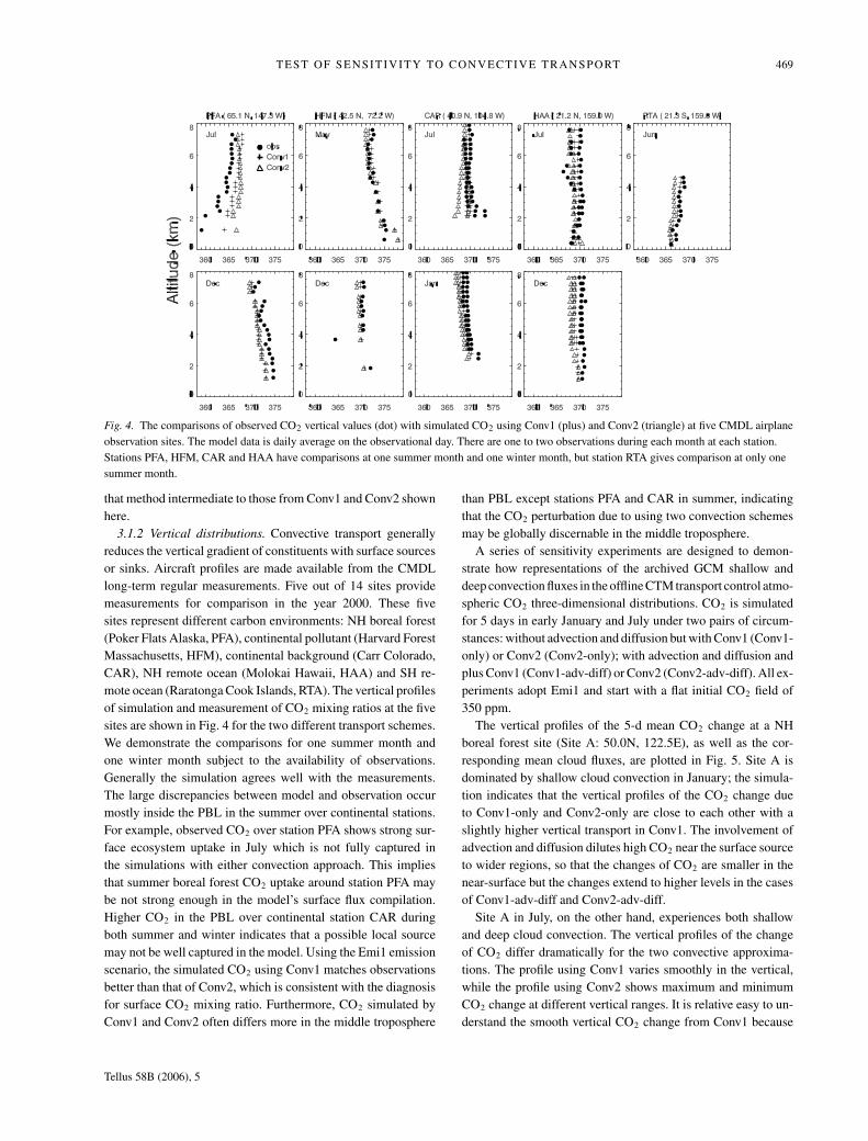
TEST OF SENSITIVITY TO CONVECTIVE TRANSPORT 469

Fig. 4. The comparisons of observed CO2 vertical values (dot) with simulated CO2 using Conv1 (plus) and Conv2 (triangle) at five CMDL airplane

observation sites. The model data is daily average on the observational day. There are one to two observations during each month at each station.

Stations PFA, HFM, CAR and HAA have comparisons at one summer month and one winter month, but station RTA gives comparison at only one

summer month.

that method intermediate to those from Conv1 and Conv2 shown

here.

3.1.2 Vertical distributions. Convective transport generally

reduces the vertical gradient of constituents with surface sources

or sinks. Aircraft profiles are made available from the CMDL

long-term regular measurements. Five out of 14 sites provide

measurements for comparison in the year 2000. These five

sites represent different carbon environments: NH boreal forest

(Poker Flats Alaska, PFA), continental pollutant (Harvard Forest

Massachusetts, HFM), continental background (Carr Colorado,

CAR), NH remote ocean (Molokai Hawaii, HAA) and SH re-

mote ocean (Raratonga Cook Islands, RTA). The vertical profiles

of simulation and measurement of CO2 mixing ratios at the five

sites are shown in Fig. 4 for the two different transport schemes.

We demonstrate the comparisons for one summer month and

one winter month subject to the availability of observations.

Generally the simulation agrees well with the measurements.

The large discrepancies between model and observation occur

mostly inside the PBL in the summer over continental stations.

For example, observed CO2 over station PFA shows strong sur-

face ecosystem uptake in July which is not fully captured in

the simulations with either convection approach. This implies

that summer boreal forest CO2 uptake around station PFA may

be not strong enough in the model’s surface flux compilation.

Higher CO2 in the PBL over continental station CAR during

both summer and winter indicates that a possible local source

may not be well captured in the model. Using the Emi1 emission

scenario, the simulated CO2 using Conv1 matches observations

better than that of Conv2, which is consistent with the diagnosis

for surface CO2 mixing ratio. Furthermore, CO2 simulated by

Conv1 and Conv2 often differs more in the middle troposphere

than PBL except stations PFA and CAR in summer, indicating

that the CO2 perturbation due to using two convection schemes

may be globally discernable in the middle troposphere.

A series of sensitivity experiments are designed to demon-

strate how representations of the archived GCM shallow and

deep convection fluxes in the offline CTM transport control atmo-

spheric CO2 three-dimensional distributions. CO2 is simulated

for 5 days in early January and July under two pairs of circum-

stances: without advection and diffusion but with Conv1 (Conv1-

only) or Conv2 (Conv2-only); with advection and diffusion and

plus Conv1 (Conv1-adv-diff) or Conv2 (Conv2-adv-diff). All ex-

periments adopt Emi1 and start with a flat initial CO2 field of

350 ppm.

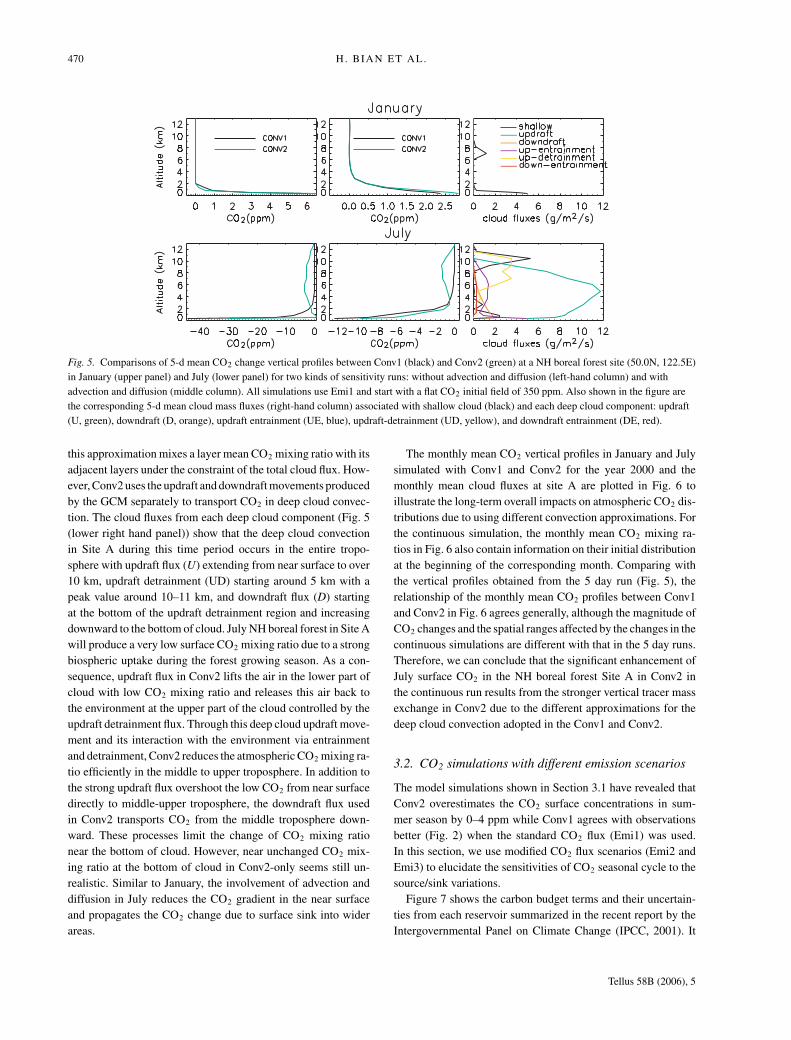
The vertical profiles of the 5-d mean CO2 change at a NH

boreal forest site (Site A: 50.0N, 122.5E), as well as the cor-

responding mean cloud fluxes, are plotted in Fig. 5. Site A is

dominated by shallow cloud convection in January; the simula-

tion indicates that the vertical profiles of the CO2 change due

to Conv1-only and Conv2-only are close to each other with a

slightly higher vertical transport in Conv1. The involvement of

advection and diffusion dilutes high CO2 near the surface source

to wider regions, so that the changes of CO2 are smaller in the

near-surface but the changes extend to higher levels in the cases

of Conv1-adv-diff and Conv2-adv-diff.

Site A in July, on the other hand, experiences both shallow

and deep cloud convection. The vertical profiles of the change

of CO2 differ dramatically for the two convective approxima-

tions. The profile using Conv1 varies smoothly in the vertical,

while the profile using Conv2 shows maximum and minimum

CO2 change at different vertical ranges. It is relative easy to un-

derstand the smooth vertical CO2 change from Conv1 because

Tellus 58B (2006), 5

470 H. BIAN ET AL.

Fig. 5. Comparisons of 5-d mean CO2 change vertical profiles between Conv1 (black) and Conv2 (green) at a NH boreal forest site (50.0N, 122.5E)

in January (upper panel) and July (lower panel) for two kinds of sensitivity runs: without advection and diffusion (left-hand column) and with

advection and diffusion (middle column). All simulations use Emi1 and start with a flat CO2 initial field of 350 ppm. Also shown in the figure are

the corresponding 5-d mean cloud mass fluxes (right-hand column) associated with shallow cloud (black) and each deep cloud component: updraft

(U, green), downdraft (D, orange), updraft entrainment (UE, blue), updraft-detrainment (UD, yellow), and downdraft entrainment (DE, red).

this approximation mixes a layer mean CO2 mixing ratio with its

adjacent layers under the constraint of the total cloud flux. How-

ever, Conv2 uses the updraft and downdraft movements produced

by the GCM separately to transport CO2 in deep cloud convec-

tion. The cloud fluxes from each deep cloud component (Fig. 5

(lower right hand panel)) show that the deep cloud convection

in Site A during this time period occurs in the entire tropo-

sphere with updraft flux (U) extending from near surface to over

10 km, updraft detrainment (UD) starting around 5 km with a

peak value around 10–11 km, and downdraft flux (D) starting

at the bottom of the updraft detrainment region and increasing

downward to the bottom of cloud. July NH boreal forest in Site A

will produce a very low surface CO2 mixing ratio due to a strong

biospheric uptake during the forest growing season. As a con-

sequence, updraft flux in Conv2 lifts the air in the lower part of

cloud with low CO2 mixing ratio and releases this air back to

the environment at the upper part of the cloud controlled by the

updraft detrainment flux. Through this deep cloud updraft move-

ment and its interaction with the environment via entrainment

and detrainment, Conv2 reduces the atmospheric CO2 mixing ra-

tio efficiently in the middle to upper troposphere. In addition to

the strong updraft flux overshoot the low CO2 from near surface

directly to middle-upper troposphere, the downdraft flux used

in Conv2 transports CO2 from the middle troposphere down-

ward. These processes limit the change of CO2 mixing ratio

near the bottom of cloud. However, near unchanged CO2 mix-

ing ratio at the bottom of cloud in Conv2-only seems still un-

realistic. Similar to January, the involvement of advection and

diffusion in July reduces the CO2 gradient in the near surface

and propagates the CO2 change due to surface sink into wider

areas.

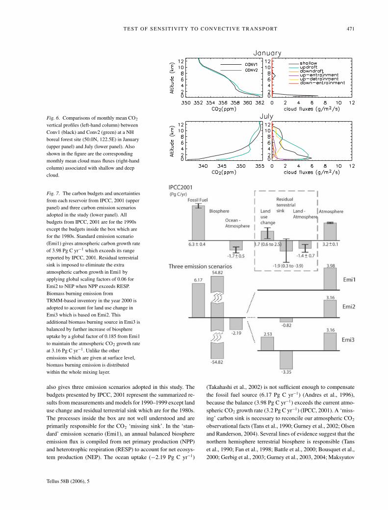
The monthly mean CO2 vertical profiles in January and July

simulated with Conv1 and Conv2 for the year 2000 and the

monthly mean cloud fluxes at site A are plotted in Fig. 6 to

illustrate the long-term overall impacts on atmospheric CO2 dis-

tributions due to using different convection approximations. For

the continuous simulation, the monthly mean CO2 mixing ra-

tios in Fig. 6 also contain information on their initial distribution

at the beginning of the corresponding month. Comparing with

the vertical profiles obtained from the 5 day run (Fig. 5), the

relationship of the monthly mean CO2 profiles between Conv1

and Conv2 in Fig. 6 agrees generally, although the magnitude of

CO2 changes and the spatial ranges affected by the changes in the

continuous simulations are different with that in the 5 day runs.

Therefore, we can conclude that the significant enhancement of

July surface CO2 in the NH boreal forest Site A in Conv2 in

the continuous run results from the stronger vertical tracer mass

exchange in Conv2 due to the different approximations for the

deep cloud convection adopted in the Conv1 and Conv2.

3.2. CO2 simulations with different emission scenarios

The model simulations shown in Section 3.1 have revealed that

Conv2 overestimates the CO2 surface concentrations in sum-

mer season by 0–4 ppm while Conv1 agrees with observations

better (Fig. 2) when the standard CO2 flux (Emi1) was used.

In this section, we use modified CO2 flux scenarios (Emi2 and

Emi3) to elucidate the sensitivities of CO2 seasonal cycle to the

source/sink variations.

Figure 7 shows the carbon budget terms and their uncertain-

ties from each reservoir summarized in the recent report by the

Intergovernmental Panel on Climate Change (IPCC, 2001). It

Tellus 58B (2006), 5

TEST OF SENSITIVITY TO CONVECTIVE TRANSPORT 471

Fig. 6. Comparisons of monthly mean CO2

vertical profiles (left-hand column) between

Conv1 (black) and Conv2 (green) at a NH

boreal forest site (50.0N, 122.5E) in January

(upper panel) and July (lower panel). Also

shown in the figure are the corresponding

monthly mean cloud mass fluxes (right-hand

column) associated with shallow and deep

cloud.

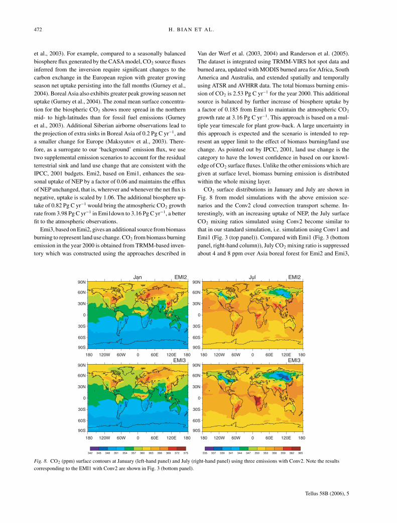
Fig. 7. The carbon budgets and uncertainties

from each reservoir from IPCC, 2001 (upper

panel) and three carbon emission scenarios

adopted in the study (lower panel). All

budgets from IPCC, 2001 are for the 1990s

except the budgets inside the box which are

for the 1980s. Standard emission scenario

(Emi1) gives atmospheric carbon growth rate

of 3.98 Pg C yr−1 which exceeds its range

reported by IPCC, 2001. Residual terrestrial

sink is imposed to eliminate the extra

atmospheric carbon growth in Emi1 by

applying global scaling factors of 0.06 for

Emi2 to NEP when NPP exceeds RESP.

Biomass burning emission from

TRMM-based inventory in the year 2000 is

adopted to account for land use change in

Emi3 which is based on Emi2. This

additional biomass burning source in Emi3 is

balanced by further increase of biosphere

uptake by a global factor of 0.185 from Emi1

to maintain the atmospheric CO2 growth rate

at 3.16 Pg C yr−1. Unlike the other

emissions which are given at surface level,

biomass burning emission is distributed

within the whole mixing layer.

also gives three emission scenarios adopted in this study. The

budgets presented by IPCC, 2001 represent the summarized re-

sults from measurements and models for 1990–1999 except land

use change and residual terrestrial sink which are for the 1980s.

The processes inside the box are not well understood and are

primarily responsible for the CO2 ‘missing sink’. In the ‘stan-

dard’ emission scenario (Emi1), an annual balanced biosphere

emission flux is compiled from net primary production (NPP)

and heterotrophic respiration (RESP) to account for net ecosys-

tem production (NEP). The ocean uptake (−2.19 Pg C yr−1)

(Takahashi et al., 2002) is not sufficient enough to compensate

the fossil fuel source (6.17 Pg C yr−1) (Andres et al., 1996),

because the balance (3.98 Pg C yr−1) exceeds the current atmo-

spheric CO2 growth rate (3.2 Pg C yr−1) (IPCC, 2001). A ‘miss-

ing’ carbon sink is necessary to reconcile our atmospheric CO2

observational facts (Tans et al., 1990; Gurney et al., 2002; Olsen

and Randerson, 2004). Several lines of evidence suggest that the

northern hemisphere terrestrial biosphere is responsible (Tans

et al., 1990; Fan et al., 1998; Battle et al., 2000; Bousquet et al.,

2000; Gerbig et al., 2003; Gurney et al., 2003, 2004; Maksyutov

Tellus 58B (2006), 5

472 H. BIAN ET AL.

et al., 2003). For example, compared to a seasonally balanced

biosphere flux generated by the CASA model, CO2 source fluxes

inferred from the inversion require significant changes to the

carbon exchange in the European region with greater growing

season net uptake persisting into the fall months (Gurney et al.,

2004). Boreal Asia also exhibits greater peak growing season net

uptake (Gurney et al., 2004). The zonal mean surface concentra-

tion for the biospheric CO2 shows more spread in the northern

mid- to high-latitudes than for fossil fuel emissions (Gurney

et al., 2003). Additional Siberian airborne observations lead to

the projection of extra sinks in Boreal Asia of 0.2 Pg C yr−1, and

a smaller change for Europe (Maksyutov et al., 2003). There-

fore, as a surrogate to our ‘background’ emission flux, we use

two supplemental emission scenarios to account for the residual

terrestrial sink and land use change that are consistent with the

IPCC, 2001 budgets. Emi2, based on Emi1, enhances the sea-

sonal uptake of NEP by a factor of 0.06 and maintains the efflux

of NEP unchanged, that is, wherever and whenever the net flux is

negative, uptake is scaled by 1.06. The additional biosphere up-

take of 0.82 Pg C yr−1 would bring the atmospheric CO2 growth

rate from 3.98 Pg C yr−1 in Emi1down to 3.16 Pg C yr−1, a better

fit to the atmospheric observations.

Emi3, based on Emi2, gives an additional source from biomass

burning to represent land use change. CO2 from biomass burning

emission in the year 2000 is obtained from TRMM-based inven-

tory which was constructed using the approaches described in

Jan EMI2

180 120W 60W 0 60E 120E 180

90S

60S

30S

0

30N

60N

90N Jul EMI2

180 120W 60W 0 60E 120E 180

90S

60S

30S

0

30N

60N

90N

EMI3

180 120W 60W 0 60E 120E 180

90S

60S

30S

0

30N

60N

90N

342 345 348 351 354 357 360 363 366 369 372 375

EMI3

180 120W 60W 0 60E 120E 180

90S

60S

30S

0

30N

60N

90N

335 337 339 341 344 347 350 353 356 359 362 365

Fig. 8. CO2 (ppm) surface contours at January (left-hand panel) and July (right-hand panel) using three emissions with Conv2. Note the results

corresponding to the EMI1 with Conv2 are shown in Fig. 3 (bottom panel).

Van der Werf et al. (2003, 2004) and Randerson et al. (2005).

The dataset is integrated using TRMM-VIRS hot spot data and

burned area, updated with MODIS burned area for Africa, South

America and Australia, and extended spatially and temporally

using ATSR and AVHRR data. The total biomass burning emis-

sion of CO2 is 2.53 Pg C yr−1 for the year 2000. This additional

source is balanced by further increase of biosphere uptake by

a factor of 0.185 from Emi1 to maintain the atmospheric CO2

growth rate at 3.16 Pg C yr−1. This approach is based on a mul-

tiple year timescale for plant grow-back. A large uncertainty in

this approach is expected and the scenario is intended to rep-

resent an upper limit to the effect of biomass burning/land use

change. As pointed out by IPCC, 2001, land use change is the

category to have the lowest confidence in based on our knowl-

edge of CO2 surface fluxes. Unlike the other emissions which are

given at surface level, biomass burning emission is distributed

within the whole mixing layer.

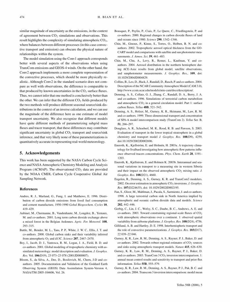
CO2 surface distributions in January and July are shown in

Fig. 8 from model simulations with the above emission sce-

narios and the Conv2 cloud convection transport scheme. In-

terestingly, with an increasing uptake of NEP, the July surface

CO2 mixing ratios simulated using Conv2 become similar to

that in our standard simulation, i.e. simulation using Conv1 and

Emi1 (Fig. 3 (top panel)). Compared with Emi1 (Fig. 3 (bottom

panel, right-hand column)), July CO2 mixing ratio is suppressed

about 4 and 8 ppm over Asia boreal forest for Emi2 and Emi3,

Tellus 58B (2006), 5

TEST OF SENSITIVITY TO CONVECTIVE TRANSPORT 473

Fig. 9. Same as Fig. 2, but using three

emissions with Conv2. Note the result

corresponding to EMI1 with Conv2 is shown

in Fig. 2 (right-hand column).

respectively (Fig. 8). Furthermore, adjustment of the NH bio-

sphere flux exhibits global implications: global surface CO2 in

July is decreased due to the stronger biosphere uptake except in

regions with local fossil fuel and/or biomass burning emissions.

In January, the CO2 surface mixing ratios from the Emi1 and

Emi2 emission scenarios are similar except over the SH forest

regions (south America, south Africa and Australia) where CO2

from Emi2 (Fig. 8 (top panel, left-hand column)) is about 0.2 ppm

lower than that from Emi1 (Fig. 3 (bottom panel, left-hand col-

umn)) due to the increase of CO2 loss in the SH growing season.

Since Emi3 includes biomass burning emission, the CO2 dis-

crepancy between Emi1 and Emi3 is larger than between Emi1

and Emi2, but the difference is still less than 1 ppm.

Simulated surface CO2 mixing ratios with three emissions are

also compared with CMDL observations in Fig. 9. The discrep-

ancies identified in Section 3.1 with using Emi1 have now be-

come reduced or disappeared with the use of Emi3. Specifically,

the improvement has happened at the stations in NH middle and

high latitudes, such as ALT. The improvement at these stations in

July is attributed to the enhancement of CO2 uptake in NH boreal

forests. The adjustment of biomass burning brings a slightly bet-

ter agreement in model-observation comparison in station ASC.

However, the misrepresentation of tracer concentration during

ITCZ at station SEY remains.

4. Conclusions

Quantification of the uncertainty of model behaviour is essential

although the acceptable level of uncertainty depends on the ap-

plication. We present in this paper an evaluation of uncertainties

of convective transport parameterization by using two different

implementation schemes in a single offline CTM framework,

driven by the same meteorological fields. The referred two meth-

ods represent cloud convective transport from a simple form to a

more complex form. The discrepancies arising from the different

approaches are the largest in the NH middle latitudes in summer

season, which is attributed primarily to the season’s deep cloud

activities that are represented differently in the two approaches.

It confirms and explains the previous finding from TransCom-3

that the model results vary the most during the growing season

(summer) in the northern land regions (Gurney et al., 2004).

Furthermore, the largest discrepancy between Conv1 and Conv2

is 7.8 ppm of CO2, which is about 30% of the CO2 seasonal-

ity for that area. The message conveyed from our study is that,

even with the same archived cloud fluxes, different implemen-

tation produces substantial discrepancy in the CO2 distribution.

Varying methods of subgrid convective parameterization among

different models are likely to produce comparable or even larger

differences. This reinforces the crucial importance of quantify-

ing the convective transport error in CO2 simulations.

Our work also shows that the impact of convection error de-

pends not only on the representation of convection cloud trans-

port in a model, but also on the collocation of deep cloud con-

vection and tracer surface fluxes. Therefore, it is not sufficient to

estimate the convection uncertainty for CO2 simulation through

the use of inert tracers with known emissions and atmospheric

observations, such as Rn and SF6. We need to use CO2 itself.

The emission scenario complied by TransCom 3 and two al-

ternate emission scenarios based on IPCC, 2001 are used to

address how these transport uncertainties compare to those in

CO2 source and sink distributions. The investigation indicates

that differences between the convective transport forms have

Tellus 58B (2006), 5

474 H. BIAN ET AL.

similar magnitude of uncertainty as the emissions, in the context

of agreement between CO2 simulations and observations. This

result highlights the complexity of simulating atmospheric CO2,

where balances between different processes (in this case convec-

tive transport and emission) can obscure the physical nature of

relationships within the system.

The model simulation using the Conv1 approach corresponds

better with several aspects of the observations when using

TransCom emissions and GEOS-4 winds. On the other hand, the

Conv2 approach implements a more complete representation of

the convective processes, which should be more physically re-

alistic. Although Conv2 in the standard scenario does not com-

pare as well with observations, the difference is comparable to

that produced by known uncertainties in the CO2 surface fluxes.

Thus, we cannot infer that one method is conclusively better than

the other. We can infer that the different CO2 fields produced by

the two methods will produce different seasonal source/sink dis-

tributions in the context of an inverse calculation, and we can use

the magnitude of the difference here as one estimate of model

transport uncertainty. We also recognize that different models

have quite different methods of parameterizing subgrid mass

fluxes and tracer transport, that these differences may contribute

significant uncertainty in global CO2 transport and source/sink

inference, and that very likely none of these parameterizations is

quantitatively accurate in representing real-world meteorology.

5. Acknowledgements

This work has been supported by the NASA Carbon Cycle Sci-

ence and NASA Atmospheric Chemistry Modeling and Analysis

Program (ACMAP). The observational CO2 data are provided

by the NOAA CMDL Carbon Cycle Cooperative Global Air

Sampling Network.

References

Andres, R. J., Marland, G., Fung, I. and Matthews, E. 1996. Distri-

bution of carbon dioxide emissions from fossil fuel consumption

and cement manufacture, 1950-1990 Gobal Biogeochem. Cycles 10,

419–429.

Aubinet, M., Chermanne, B., Vandenhaute, M., Longdoz, B., Yernaux,

M. and co-authors. 2001. Long term carbon dioxide exchange above

a mixed forest in the Belgian Ardennes. Agric. For. Meteorol. 108,

293–315.

Battle, M., Bender, M. L., Tans, P. P., White, J. W. C., Ellis, J. T. and

co-authors. 2000. Global carbon sinks and their variability inferred

from atmospheric O2 and d13C. Science 287, 2467–2470.

Bey, I., Jacob, D. J., Yantosca, R. M., Logan, J. A., Field, B. D. and

co-authors. 2001. Global modeling of tropospheric chemistry with as-

similated meteorology: model description and evaluation. J. Geophys.Res. Vol. 106(D19), 23 073–23 078 (2001JD000807).

Bloom, S., da Silva, A., Dee, D., Bosilovich, M., Chern, J-D and co-

authors. 2005. Documentation and Validation of the Goddard Earth

Observing System (GEOS) Data Assimilation System-Version 4,

NASA/TM-2005-104606, Vol. 26.

Bousquet, P., Peylin, P., Ciais, P., Le Quere, C., Friedlingstein, P. and

co-authors. 2000. Regional changes in carbon dioxide fluxes of land

and oceans since 1980. Science 290, 1342–1346.

Chin, M., Ginoux, P., Kinne, S., Torres, O., Holben, B. N. and co-

authors. 2002. Tropospheric aerosol optical thickness from the GO-

CART model and comparisons with satellite and sun photometer mea-

surements. J. Atmos. Sci. 59, 461–483.

Chin, M., Chu, A., Levy, R., Remer, L., Kaufman, Y. and co-

authors. 2004. Aerosol distribution in the northern hemisphere dur-

ing ACE-Asia: results from global model, satellite observations,

and sunphotometer measurements. J. Geophys. Res., 109, doi:

10.1029/2004JD004829.

Collins, B., Leo, D., Hack, J., Randall, D., Rasch, P. and co-authors. 2004.

Description of the NCAR Community Atmosphere Model (CAM 3.0),

http://www.ccsm.ucar.edu/models/atm-cam/docs/description/.

Denning, A. S., Collatz, G. J., Zhang, C., Randall, D. A., Berry, J. A.

and co-authors. 1996. Simulations of terrestrial carbon metabolism

and atmospheric CO2 in a general circulation model. Part 1: surface

carbon fluxes. Tellus 48B, 521–542.

Denning, A. S., Holzer, M., Gurney, K. R., Heimann, M., Law, R. M.

and co-authors. 1999. Three-dimensional transport and concentration

of SF6-A model intercomparison study (TransCom 2). Tellus Ser. B,

51, 266–297.

Douglass, A. R., Schoeberl, M. R., Rood, R. B. and Pawson, S. 2003.

Evaluation of transport in the lower tropical stratosphere in a global

chemistry and transport model J. Geophys. Res. 108(D9), 4259,

doi:10.1029/2002JD002696.

Eneroth, K., Kjellstrom, E. and Holmen, H. 2003a. A trajectory clima-

tology for Svalbard investigating how atmospheric flow patterns influ-

ence observed tracers concentrations. Phys. Chem. Earth 28, 1191–

1203.

Eneroth, K., Kjellstrom, E. and Holmen K. 2003b. Interannual and sea-

sonal variations in transport to a measuring site in western Siberia

and their impact on the observed atmospheric CO2 mixing ratio. J.Geophys. Res. 108(D21), 4660.

Engelen, R., Denning, A. S., Gurney, K. R. and TransCom3 modelers.

2002. On error estimation in atmospheric CO2 inversions. J. Geophys.Res. 107(D224635), doi: 10.1029/2002JD002195.

Fan, S., Gloor, M., Mahlman, J., Pacala, S., Sarmiento, J. and co-authors.

1998. A large terrestrial carbon sink in North America implied by

atmospheric and oceanic carbon dioxide data and models. Science282, 442–446.

Gerbig, C., Lin, J. C., Wofsy, S. C., Daube, B. C., Andrews, A. E. and

co-authors. 2003. Toward constraining regional-scale fluxes of CO2

with atmospheric observations over a continent. 1: observed spatial

variability from airborne platforms. J. Geophys. Res. 108(D24), 4756.

Gilliland, A. B. and Hartley, D. E. 1998. Interhemispheric transport and

the role of convective parameterizations. J. Geophys. Res. 103(D17),

22 039–22 046.

Gurney, K. R., Law, R. M., Denning, A. S., Rayner, P. J., Baker, D. and

co-authors. 2002. Towards robust regional estimates of CO2 sources

and sinks using atmospheric transport models. Nature 415, 626–630.

Gurney, K. R., Law, R. M., Denning, A. S., Rayner, P. J., Baker, D.

and co-authors. 2003. TransCom 3 CO2 inversion intercomparison. 1:

annual mean control results and sensitivity to transport and prior flux

information. Tellus 55B, 555–579.

Gurney, K. R., Law, R. M., Denning, A. S., Rayner, P. J., Pak, B. C. and

co-authors. 2004. Transcom 3 inversion intercomparison: model mean

Tellus 58B (2006), 5

TEST OF SENSITIVITY TO CONVECTIVE TRANSPORT 475

results for the estimation of seasonal carbon sources and sinks. GlobalBiogeochem. Cycles 18, GB1010, doi: 10.1029/2003GB002111.

Hack, J. J. 1994. Parameterization of moist convection in the National

Center for Atmospheric Research community climate model (CCM2).

J. Geophys. Res. 99, 5551–5568.

Intergovernmental Panel on Climate Change (IPCC). 2001. Climate

Change 2001: Synthesis Report: Third Assessment Report of the Inter-

governmental Panel on Climate Change, Cambridge University Press,

New York.

Kawa, S. R., Erickson III, D. J., Pawson, S. and Zhu, Z. 2004.

Global CO2 transport simulations using meteorological data from the

NASA data assimilation system. J. Geophys. Res. 109(D18312), doi:

10.1029/2004JD004554.

Law, R. M., Rayner, P. J., Denning, A. S., Erickson, D., Fung, I. Y.

and co-authors. 1996. Variations in modeled atmospheric transport

of carbon dioxide and the consequences for CO2 inversions. GlobalBiogeochem. Cycles 10, 783–796.

Li, Q. B., Jiang, J. H., Wu, D. L., Read, W. G., Livesey, N. J. and co-

authors. 2005. Convective outflow of South Asian pollution: a global

CTM simulation compared with EOS MLS observations. Geophys.Res. Lett. 32(L14826).

Lin, S. and Rood, R. B. 1996. Multidimensional flux-form semi-

Lagrangian transport schemes. Mon. Weather Rev. 124, 2046–2070.

Mahowald, N. M., Rasch, P. J. and Prinn, R. G. 1995. Cumulus parame-

terizations in chemical transport models. J. Geophys. Res. 100(D12),

26 173–26 189.

Maksyutov, S., Machida, T., Mukai, H., Patra, P. K., Nakazawa, T. and

TransCom 3 modelers. 2003. Effect of recent observations on Asian

CO2 flux estimates by transport model inversions. Tellus 55B, 522–

529.

Millet, D. B., Jacob, D. J., Turquety, S., Hudman, R. C., Wu, S. and co-

authors. 2006. Formaldehyde distribution over North America: impli-

cations for satellite retrievals of formaldehyde columns and isoprene

emission. J. Geophys. Res., in press.

Murayama, S., Taguchi, S. and Higuchi, K. 2004. Internannual varia-

tion in the atmospheric CO2 growth rate: role of atmospheric trans-

port in the Northern Hemisphere. J. Geophys. Res. 109(D02305),

doi:10.1029/2003JD003729.

Olivie, D. J. L., van Velthoven, P. F. J., Beljaars, A. C. M. and Kelder, H.

M. 2004. Comparison between archived and off-line diagnosed con-

vection mass fluxes in the chemistry transport model TM3. J. Geophys.Res. 109(D11303), doi:10.1029/2003JD004036.

Olsen, S. C. and Randerson, J. T. 2004. Differences between surface and

column atmospheric CO2 and implications for carbon cycle research.

J. Geophy. Res. 109(D02301), doi:10.1029/2003JD003968.

Palmer, P. I., Jacob, D. J., Jones, D. B. A., Heald, C. L., Yantosca,

R. M. and co-authors. 2003. Inverting for emissions of carbon monox-

ide from Asia using aircraft observations over the western Pacific.

J. Geophys. Res. 108(D21), 8828, doi:10.1029/2003JD003397.

Randerson, J. T., Thompson, M. V., Conway, T. J., Fung, I. Y. and Field,

C. B. 1997. The contribution of terrestrial sources and sinks to trends in

the seasonal cycle of atmospheric carbon dioxide. Global Biogeochem.Cycles 11, 535–560.

Randerson, J. T., van der Werf, G. R., Collatz, G. J., Giglio, L., Still,

C. J. and co-authors. 2005. Fire emissions from C3 and C4 vegetation

and their influence on interannual variability of atmospheric CO2 and

d13CO2. Global Biogeochem. Cycles 19 (Art. no. GB2019).

Rannik, U., Aubinet, A., Kurbanmuradov, O., Sabelfeld, K. K., Markka-

nen, T. and co-authors. 2000. Footprint analysis for measurements

over a heterogeneous forest. Boundary Layer Meteorol. 97, 137–166.

Suntharalingam, P., Randerson, J. T., Krakauer, N., Jacob, D. J. and

Logan, J. A. 2005. The influence of reduced carbon emissions

and oxidation on the distribution of atmospheric CO2: implica-

tions for inversion analyses. Global Biogeochem. cycles 19(GB4003),

doi:10,1029/2005GB002466.

Takahashi, T., Sutherland, S. C., Sweeney, C., Poisson, A., Metzl, N. and

co-authors. 2002. Global sea-air CO2 flux based on climatological

surface ocean pCO2, and seasonal biological and temperature effects,

Deep-Sea Res. II 49, 1601–1622.

Tans, P. P., Fung, I. Y. and Takahashi, T. 1990. Observational constraints

on the global atmospheric CO2 budget. Science 247, 1431–1438.

Van der Werf, G. R., Randerson, J. T., Collatz, G. J. and Giglio, L. 2003.

Carbon emissions from fires in tropical and subtropical ecosystems.

Global Change Biol. 9, 547–562.

Van der Werf, G. R., Randerson, J. T., Collatz, G. J., Giglio, L.,

Kasibhatla, P. S. and co-authors. Continental-scale partitioning of fire

emissions during the 1997–2001 El Nino/La Nino period. Science 303,

73–76.

Yi, C., Davis, K. J., Bakwin, P. S., Denning, A. S., Zhang, N.

and co-authors. 2004. Observed covariance between ecosystem

carbon exchange and atmospheric boundary layer dynamics at

a site in northern Wisconsin. J. Geophys. Res. 109(D08302),

doi:10.1029/2003JD004164.

Zender, C. S., Bian, H. and Newman, D. 2003. The mineral dust en-

trainment and deposition (DEAD) model: description and global dust

distribution J. Geophys. Res. 108, 4416.

Zhang, G. J. and McFarlane, N. A. 1995. Sensitivity of climate simu-

lations to the parameterization of cumulus convection in the Cana-

dian climate center general-circulation model. Atmos. Ocean 33,

407–446.

Tellus 58B (2006), 5