Embed Size (px)
Citation preview
Journal of Public Economics 19 (1982) 311-331. North-Holland Publishing Company
A TEST FOR ALLOCATIVE EFFICIENCY IN THE LOCAL PUBLIC SECTOR
Jan K. BRUECKNER
University of Illinois, Urbana, IL 61801, USA
Received October 1981, revised version received January 1982
This paper develops a test for Pareto-elliciency in the local public sector using the analytical result that aggregate property value is maximized at the public output level which satisfies the Samuelson condition for efficiency. By using cross-section data, it is possible to deduce whether a representative community provides its public goods in a property-value-maximizing (and hence efficient) fashion. The empirical results show no systematic tendency to either under- or over- provide public goods in a sample of Massachusetts communities.
1. Introduction
Although allocative efficiency in the public sector has been a central theoretical concern in public finance ever since the pioneering study of Samuelson (1954), the positive question of whether real-world public outputs are in fact efficient has received much less attention. In a rare attempt to address this issue, Barlow (1970) invoked an ingenious argument based on the median voter model to conclude that expenditure on education in his sample was above the efficient level. The present paper offers an entirely different efficiency test. The present test is based on the theoretical result that aggregate property value in a community which levies a property tax is an inverted U-shaped function of its public good output, with the maximum occurring at the output level which satisfies the Samuelson condition for Pareto-efficiency [see Brueckner (1979, 1980)]. Using this result, it follows that if a community’s aggregate property value is insensitive to a marginal change in its public good output, then the good is provided at a Pareto- efficient level. A cross-section regression relating aggregate property values to public expenditures and other variables for a sample of Massachusetts communities forms the basis for the efficiency test. Properly interpreted, the regression results show the response of aggregate property value in a representative community to a change in its public good output, allowing an appraisal of efficiency.’
‘While the present paper is concerned with the efficiency of real-world public outputs, the principle of property value maximization can also be used to generate a decision rule for local
0047-2727/82/OOOCrOOOO/$O2.75 0 1982 North-Holland
Most previous empirical work on property values and public goods c\tcnds the seminal study of Oates (1969) who showed that median property value is positively influenced by a community’s level of public spending.
Oates and many of his followers viewed this empirical finding as an affirmation of the Tiebout hypothesis (1956), which states that consumers migrate in response to fiscal differentials and that such migration tends to generate homogenous communities, guaranteeing Pareto-efficient provision of local public goods. A proper interpretation of the Oates finding, however, relates only to the first of these claims: empirical results which show by the presence of a capitalization effect that consumers value public goods establish that the preconditions for ‘voting with one’s feet’ exist but do not prove that the migration process will lead to an efficient Tiebout equilibrium.’ This narrow view of the Oates finding, which is consistent with recent theoretical attacks on Tiebout [see, for example, Stiglitz (1977)], underlies the recent empirical study of Brueckner (1979). Recognizing the possibility of public sector inefficiency due to failure of the Tiebout mechanism, Brueckner showed using the principles described above that a properly specified Oates- style regression can indicate whether public outputs are Pareto-efficient in communities whose populations are heterogenous due to incomplete adjustment toward a Tiebout equilibrium. By showing that a property value regression contains a hidden verdict on the efficiency of public outputs in a non-Tiebout world, the Brueckner paper essentially stood the Oates tradition on its head. Unfortunately, since the paper’s efficiency argument relied on the
relationship between aggregate property value and public spending, while the regression used the median value dependent variable to stress the link with Oates, precise interpretation of the empirical results required a forbiddingly complex argument. By using the ideal dependent variable (aggregate property
value) as well as an optimal data set, the present paper eliminates all the difficulties inherent in the previous study. The simplicity and generality of the property value approach to evaluating public sector efficiency emerges in a clear fashion.
In the next section of the paper a theoretical model of property value determination under property taxation similar to that of Brueckner (1979) is developed and the relationship between property values and public outputs is derived. Subsequent sections of the paper describe the estimation problem and present the empirical results and final conclusions.
governments. Brueckner (1980) showed that when each local government chooses its public output to maximize aggregate property value, the resulting community system equilibrium has desirable efficiency properties. For a related treatment, see Sonstelie and Portney (1978).
‘A more natural test for the operation of the Tiebout mechanism would examine the degree of homogeneity of local jurisdictions. For recent papers pursuing this approach, see Eberts and Gronberg (1981) and Pack and Pack (1978).
J.K. Brueckner, Allocative eficiency in the public sector 313
2. Analysis
The first assumption underlying the analysis is that consumers have identical tastes. While this requirement is somewhat unrealistic, no empirical study of the relation between property values and public spending can proceed without it. Utility is assumed to depend on the consumption of four commodities: housing services (cJ), two public goods (zl and z,), and a numeraire composite commodity (x). It is assumed that the common utility function u(zl, z2, 4, x) is strictly quasi-concave. Two public goods are included
in the model for realism; in the empirical work, the public goods are education and a composite of municipal services such as fire and police
protection. A further strong assumption is that utility is uniform across the system of
communities under consideration for the members of each income group. Letting U denote the utility level achieved by an individual in equilibrium, this assumption means that C=h(y), where y is the individual’s income and h is some function. Although the equilibrium relationship between utility and income is not explained within the model, the assumption h’ >O (wealthier people reach higher utilities) is natural. It should be noted that the assumption of uniform utilities within income groups makes sense only in the absence of market frictions. Unless a consumer is free to move to another community or to change his consumption bundle within a given community, the assumption will be inaccurate.
The first step in the analysis is the use of a bid-rent model to determine house rent as a function of housing characteristics. The basic idea behind this type of model is that rents must vary across houses in such a way that consumers reach the same utility level regardless of where they live. The rent for an attractive house (one with a high q or high public consumption levels) must be higher than that for a less attractive house to ensure that the occupant of the latter house enjoys higher non-housing consumption than his neighbor and is therefore able to reach the same utility level. The formal derivation begins by noting that since a consumer with income y is assumed to achieve utility h(y), his consumption bundle must satisfy
4z,> z2,4> 4 = MY).
The rent R for a dwelling which affords given consumption levels of the
public goods and housing must adjust (altering x consumption) so that (1) holds. Since the consumer’s budget constraint may be written x+ R=Y, it follows that R must satisfy
u(z,, zz> 4, Y -R) = NY).
314 J.K. Brueckner, Allocative effciency in the public sector
Eq. (2) implicitly determines the consumer bid-rent function
R = Rk,, ~294; YX (3)
which gives the house rent consistent with the assumed utility level as a function of public consumption levels, house size, and income. The fact that attractive houses command high rents follows from differentiating (2), which
gives
Rj(z,,z2,q;y)=
u~(w~~>Y--R)>~
dz,,z,>q,y-RR) '
j= 1,2,3 (4)
(subscripts denote partial derivatives). Eq. (4) shows that rent must increase, reducing x consumption, to cancel the utility-increasing effect of a higher zr, z2, or q. Note that the magnitude of the required rent increase depends on the MRS between the given commodity and x. The effect of income on rent is ambiguous under the bid-rent model (R, = 1 -h’/uq$O)
since an increase in y increases both sides of (2), making the required change in R uncertain. Note that since housing consumption is held fixed as income
increases, the effect of an income change on housing expenditure is different from the standard income effect. Finally, it is easy to show that the strict quasi-concavity of the utility function means that R is a strictly concave function of zr, z2, and q.
It is important to realize that for fixed zr and z2, (3) gives the constant- utility rent payment as a function of q without specifying the house size actually chosen by the consumer. Housing consumption will, of course, depend on the consumer’s income level and will be influenced in addition by the levels of the public goods. Therefore, the arguments of R must be viewed as interdependent, with strong positive correlations among the variables likely.3 It will become clear below that for the purposes of the analysis, the exact nature of this correlation is unimportant; the crucial observation is that house rent must be related to zr, z2, q, and y in the manner described by (3) regardless of the degree of association among the latter variables.4
The next important assumption is that tax revenue is raised entirely by property taxation using separate property tax rates r1 and r2 for the two
‘Although no attempt is made to describe the political process by which public good levels are set, it is natural that z, and z2 would increase with the income level of the community. This is a further reason to anticipate strong positive correlation among the arguments of R.
41n this context it is important to note that the consumer inhabiting a given house must offer the highest bid for it. Letting 4, and yi denote house size and income for some consumer i, this means that R(z,,z,,qi;yi) must exceed or equal R(~,,z,,q,;y~), j#i, where z1 and z2 are the public good levels for i’s community. With a continuum of income levels, i will be the highest bidder only when R,(z,, z2, qi; yi) = 0.. Without a continuum of incomes, however, i’s bid canbe maximal without satisfaction of R,=O. Thus, even when R, is evaluated at the level of 4 actually consumed, its sign remains ambiguous.
J.K. Brueckner, Allocatioe efficiency in the public sector 315
public goods. This assumption is faithful to reality for the chosen sample since Massachusetts communities levy no sales or income taxes. Now the
value (or selling price) of a rental property equals the present discounted value of the excess of rent over the property tax liability. Letting u represent value, it follows that
vJ-h +z,b e ’ (5)
where 8 is the discount rate.5 Rearrangement gives the value of a house as a function of zr, z2, q, y, and the property tax rates:
Using (6), the aggregate value of rental property in a community with n houses may be written
n c R(z,, ~2, qi; YJ 3 p i=l e+7,+z2 ’
.
Although the discussion so far applies to rental houses, the same results hold with owner-occupied dwellings. This follows because in equilibrium an
owner-occupier must be indifferent between owning and renting his house. Indifference requires that the present discounted value of rental payments R/8 equals the purchase price of the house v plus the present discounted
value of property tax payments (rl +z,)u/8. This equality reduces to (5), implying that (7) is appropriate regardless of the renter-owner-occupier
composition of the community.6
The analysis so far ignores the production side of the housing market in that aggregate value (7) is entirely demand-determined via the bid-rent function R. Although house value will in fact equal production cost in a steady-state equilibrium [making (7) superfluous], there is good reason to suppose that this link will be servered in the real-world economy, so that a demand-oriented model of house value is appropriate. To establish these points, suppose that land and capital are inputs to housing production, that the supply of land to each community is perfectly elastic at the uniform agricultural price, and that capital’s price is the same everywhere. Under these circumstances, the production cost for a house of size q will be uniform
5The formulation (5) implicitly assumes that houses have infinite lives. Incorporating the effect on value of differences in remaining lifespans among houses would introduce severe complications.
6This discussion obviously ignores the different tax treatment of owner-occupiers and renters.
316 J.K. Brueckner, Allocatioe eJicirncy in the public xctor
throughout the economy. Letting a(q) denote this cost, it then follows that in a steady-state equilibrium with zero producer profit, the value (selling price) of a house of size q in any community must equal a(q), so that house value is independent of the levels of the fiscal variables7 Since the aggregate value of residential property in a community will therefore equal xa(qJ, aggregate value will be insensitive to the public sector, being fully determined by the characteristics of the community’s housing stock. This zero-capitalization outcome is unlikely to obtain in the real world, however. The dynamic nature of the economy means that while value might equal production cost for new houses, the link between the two will be broken as time progresses, so that the value of an aging house need not equal its replacement cost. Thus, for most of the housing stock, value will be demand-determined and hence sensitive to the levels of the fiscal variables. making (7) the appropriate
aggregate expression. A variant of the preceding analysis applies to business property. Suppose
first that production uses labor as well as structure and non-structure capital but that the public goods zr and z2 do not enter firm production functions. For a given structure input s, firms (which are assumed to be identical) will maximize profit gross of rent, with the maximized value rt(s,g) depending on the structure input and the wage rate g; the price of non-structure capital (machines and intermediate goods) will be uniform across communities. Since business rents will be bid up to eliminate profits, the rent for a business
structure of size s in a community with wage rate g must equal n(s,g), implying that the structure’s value is rc(s,g)/(O+ rr + r2). Assuming that the community has m firms and using (7) the aggregate value P of residential
and business property may then be written
p=p +p zi=l + j= 1
r b Q+z,+z, e+z, +z,’
where P, stands for the aggregate value of business property.8
‘Note that the resulting absence of capitalization is due entirely to competition in the housing market. When community land areas are fixed, so that the supply of land to housing producers is perfectly inelastic, the story is somewhat different. In this case, fiscal variables may be capitalized into land rents, so that housing production costs embody fiscal effects and capitalization shows up in house prices. One might then argue that competition among community developers will lead to replication of ‘desirable’ communities until land rents everywhere equal the agricultural rent, implying the disappearance of capitalization in house prices, just as in the case where individual community land areas are flexible [see Hamilton (1976)]. It is important to realize that the absence of capitalization under this scenario does not necessarily imply public sector efficiency, contrary to the claim of Edel and Sclar (1974). Establishing that competition among community developers leads to Pareto-efficient public good outputs would require further (difftcult) analysis.
‘When firms are realistically different from one another, the function x must be indexed by firm type. For a firm of type j to occupy a given structure of size s, it must be the case that
J.K. Brueckner, Allocatioe ejjkiency in the public sector 317
The property tax system must raise revenue sufficient to finance that part
of a community’s public expenditures not supported by intergovernmental aid. Letting G, denote the intergovernmental revenue received by the community to help finance provision of public good k, budget balance for the local government requires
z,P+G,=C’(z,,n) (9)
and
z,P + G, = C2(z2, n), (10)
where the Ck are the cost functions for public production (convexity in the public outputs is assumed). The appearance of community population n in these functions reflects public good congestion; C; ~0 is appropriate if :.k is a pure public good, while C”, > 0 would hold in the presence of congestion.’
U&g (9)-and (lo), the property tax rates may be eliminated frorn the
aggregate value expression (8). First, summing (5) across i yields
P,= CR’-(r, +r,)P,
e
CR’ denotes R(z,, z2, qi; y,)]. The analogous relationship
P,= Qc’-(rr +r,)P,
e
(11)
(12)
holds for business property [rrj denotes rc(sj,g)]. Next, (9) and (10) can be added to yield (rr + z,)P = C’(z,, n) + C2(z2, n) - G, - G2. Finally, adding (11) and (12) and using the previous result to eliminate (rr +z,)(P,+ PJ give:;
.i R(z~,Z2,qi;yt)+~+G-C’(z~,~)-C2(z~,~) 5
1 1 (13)
?r’(s,g) = max {zr(s,g), i = 1,. .,1}, where I is the number of firm types. Aggregate business property value becomes ~rrf@~‘(sj,g)/(O+r, +r,), where j’(.sj) equals the index of the firm type wrth the highest value of 7[ for the given structure. Since the subsequent analysis will use aggregate business profit gross of rent (II) directly as an independent variable, the exact form of the expression which yields I7 turns out to be unimportant. Thus, whether P, in (8) or the more complex expression above is appropriate for determining aggregate value is immaterial Ibr the purposes of the analysis. In addition, note that the local wage variable g is submerged in the variable Il.
‘Since z, and z2 are represented by education and other municipal services in the empirical work, the assumption of independent cost functions is realistic. For other pairs of public goods (fire and police protection, for example), the cost of providing a given amount of one public good could depend on the level of provision of the other.
318 J.K. Brueckner, Allocative efficiency in the public sector
where n =CIZ~ is aggregate business rent and G = G, + GZ. Eq. (13) shows that aggregate property value is equal to aggregate residential and business rent plus intergovernmental aid less public good production costs, all divided
by the discount rate.
The partial derivatives of (13) with respect to variables other than the zk are
i;P 1 --‘jR,(zl>Z2: qi;Yi)‘03 ?qi
dP 1 -=HRz$(zl, z2> 4i;Yi)S”o, dYi
i=1,2 ,..., n, (15)
dP dP 1 ->o.
dn=aG=o (16)
While the above results follow automatically from (13), somewhat more
insight can be gained by referring to (8). First, it may be shown that the
partial derivatives of the zk with respect to the qi, 17, and G are all negative due to the reduction in tax effort which is possible in a community with
large houses, substantial business property, or generous intergovernmental aid. An increase in q, or Ll therefore causes an indirect increase in aggregate value through lower tax rates together with a direct increase due to higher aggregate rent [see (S)], yielding the positive expressions in (14) and (16). While an increase in G has no direct effect on rent, the indirect effect which operates through lower tax rates increases aggregate value, as shown in (16). Finally, the ambiguity of the effect of income changes on aggregate value [see (15)] follows from the uncertain effect of income on rent under the model.”
Although an increase in I7 could reflect an increase in either the size or number of business properties, finding the cffcct on value of an increase in the number of houses in the community req”uircs further analysis. First, it is
easy to see that if z1 and z2 are pure public goods (Ci = C: = 0), then any increase in n results in higher aggregate residential rent without increasing public production costs, and aggregate value in (13) increases. On the other hand, if the public goods are congested, then higher public expenditures are needed to hold the zk fixed as n increases, and the direction of change for (13) is uncertain. However, as long as the increment to rent exceeds the added
“Note that even though footnote 4 suggests that r?P/?y, will be approximately zero for all i, it is not appropriate to delete incomes from the aggregate property value relationship since (as will be seen below) utilities and hence incomes must be held constant to make efficiency inferences from the signs of iP/?z,. k = I, 2.
J.K. Brueckner, Allocative efficiency in the public sector 319
public sector costs, aggregate value will rise with n. The strong likelihood
that this condition will be satisfied suggests that a positive relationship between aggregate value and the size of the housing stock will be observed.
The nature of the relationship between aggregate property value and the levels of the public goods z, and z2 provides the basis of the test for allocative efftciency developed below. Differentiation of (13) with respect to z, and z2 yields
aP 1 n
aZ,=; i=r ( C R!f(zr, z29 4i; Yi)- ct(zk, n,
1
k= 1,2, (17)
where the last equality follows from (4). Eq. (17) establishes that (3P/8z, equals zero when the sum of the marginal rates of substitution between
public good zk and the numeraire equals the good’s marginal cost (that is, when the Samuelson condition for good zk holds). Since R is a strictly concave function of the zk and since Ck is assumed to be convex in zk, k = 1,2, it follows that P in (13) is strictly concave in the zk. The strict concavity of P means that, ceteris paribus, aggregate property value reaches a global maximum at values of z1 and z2 where both Samuelson conditions hold. This important result provides the foundation for the subsequent empirical work.
By imposing more structure on consumer tastes, it becomes possible to deduce whether the public goods exceed or fall short of their ceteris paribus property-value-maximizing levels simply by examining the signs of iP/?z,,
k= 1,2. This greatly simplifies interpretation of later empirical results. It is necessary to assume that the utility function is additively separable in z1 and
z2, so that u(z1,z2,q,x)-~(z1,q,x)+y(z2,q,x). In this case, the MRS between z1 and x is independent of z2 and the MRS between z2 and x is independent of zr, with the result that dP/az, in (17) depends only on zk, k = 1,2. This in turn means that zk is underprovided/overprovided relative to the property- value-maximizing level as dP/iiz, $0, k = I,2 Without separability of tastes, this useful conclusion need not follow.
Although (17) shows that local stationarity of aggregate value requires satisfaction of the familiar Samuelson conditions, it is important to know
precisely what efficiency implications stationarity holds. The issue is, unfortunately, not entirely straightforward due to the existence of a property tax. As shown in Brueckner (1980) using a model without business property, such a tax will distort consumer choice between housing and the numeraire x, leading to an equilibrium in which the housing stock must be viewed as non-optimal. Brueckner showed that as a result, satisfaction of the
Samuelson conditions yields only a second-best conclusion: under property taxation, satisfaction of these conditions implies that resource allocation within the community is Pareto-efficient conditional upon the non-optimal
housing stock. A similar argument would suggest that when aggregate property value is locally stationary (and hence maximal) under variation in
Z, and z2 in the present model, resource allocation is Pareto-efficient conditional upon the non-optimal stocks of residential and business
structures. That is, no rearrangement of non-structure community resources could lead to a Pareto-superior allocation.”
The fact that structures are extremely durable means that the notion of conditional efficiency is of real practical interest. While in the very long run
the stock of structures would respond to a change in the -li, the stock will be essentially frozen in place over the short term. Under these circumstances, conditional efficiency is clearly a pragmatic planning goal. At each point in time, public outputs should be chosen to yield a Pareto-optimum conditional on the (essentially fixed) stock of structures.12
Before proceeding to the empirical work, a review of the structure of the model will help clarify the connection between conditional efficiency and the behavior of property values. Fundamental to the derivation of the aggregate value relationship (13) were the assumptions that consumer utilities are fixed at equilibrium levels and business profits are zero. In essence, (13) tells how aggregate value must be related to community characteristics in order for both thcsc conditions to be satisfied. Now although (13) will therefore fit the
equilibrium data of a community system, the relationship may also be used for the conceptual exercise of determining how aggregate value in a given
community would change if z1 or z2 were increased while the utility levels of community residents and other variables were held fixed (that is, c’P/c?z,, k = 1.2, can be evaluated). Strictly speaking, this exercise. has no real-world
counterpart since other determinants of aggregate value (the qi, H, and population n) would ultimately respond to a change in the zk, as would the underlying utility levels (as mentioned above, however, the response of the stock of structures will be very slow). Nevertheless, the answer yielded by this ceteris paribus exercise is important for its efficiency implications: as stated above, if marginally increasing either z1 or z2 were to change P, then public good outputs are inefficient conditional on the community’s stock of structures. Concretely, this means that the equilibrium utilities of the
“Although the analysis of Brueckner (1980) relates to a model where the only private production activity is housing production (so that a stock of business structures does not exist), an extension of the paper‘s argument would cover the case where each community has both business and residential structures.
“It should be realized that even though the property tax will distort housing choices in a static setting, a perhaps more compelling reason for non-optimality of the stock of structures stems from the fact that buildings are very long-lived. Even in a world where no tax-induced distortions exist. imperfect foresight on the part of developers will yield housing output decisions which are non-optimal in a dynamic sense.
J.K. Brueckner, Allocative efficiency in the public sector 321
community residents, h(yi), i = 1,2,. . ., n [see (l)], are ’ suboptimal in that
reallocation of non-structure resources could increase the utility levels of some residents without reducing those of any others. Essentially, dP/dz, #O,
k = 1,2, means that the community could do better than it does in equilibrium by rearranging non-structure resources.13 Now the goal of the empirical work is to ascertain whether aP/dz,#O typically characterizes real communities. The fact that this is a ceteris paribus question poses no special problem from an empirical point of view since regression analysis applied to the equilibrium data of a community system will allow isolation of ceteris
paribus effects, as will be seen in the next section.
3. The estimation problem
Sample observations for the variables P, zl, z2, I7, G, Q, and Y (the latter are vectors representing the qi and yi) will lie somewhere on or near the aggregate property value hypersurface defined by (13) (a random error term will account for some scatter around the hypersurface).14 The goal of the empirical work is to extract information from this point scatter concerning public sector efficiency in the sample. To see how this is possible, consider
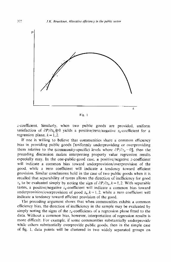
for a moment an unrealistic situation in which a single public good z is provided at different levels in a cross section of communities with identical values of Q, Y IT, and G. In this case, aggregate property value is a simple
single-peaked function of z, as shown in fig. 1. Suppose, further, that as shown in the figure, all sample observations lie to the left of the peak (that
is, aP/dz>O holds in each community). This means that the public good outputs in the sample are inefficient in the conditional sense of section 1 (holding a community’s stock of structures fixed, a higher public good output would permit a Pareto-superior allocation). Now in the situation shown in fig. 1, it is clear that a regression line fitted to the data will exhibit a positive slope. Similarly, if all observations lie to the right of the peak [public goods
are overprovided relative to the common (conditionally) efficient level], then the regression line will have a negative slope, while if observations are clustered near the peak of the curve, then the slope will be near zero. When communities realistically have different values of Q, E: Z7, and G, similar conclusions emerge: if communities uniformly satisfy dP/az $0, then a regression hyperplane fitted to the data will exhibit a positive/zero/negative
“It should be noted that this result concerns only the internd efficiency of communities. Satisfaction of the Samuelson condition in each jurisdiction is not sufficient for global optimality of the community system equilibrium (a major reorganization of community populations might improve everyone’s welfare). See Brueckner (1980).
‘%trictly speaking, references to a single hypersurface ignore the fact that the number of aquments of P will differ from community to community as a result of variation in n and consequent variation in the dimension of the vectors Q and Y Since Q and Y will be represented in the regression equation by a few summary variables, this problem disappears in practice.
322 J.K. Brueckner, Allocative efficiency in the public sector
Fig. 1
z-coefficient. Similarly, when two public goods are provided, uniform satisfaction of dP/&, $0 yields a positive/zero/negative z,-coefficient for a regression plane, k = 1,2.
If one is willing to believe that communities share a common efficiency bias in providing public goods [uniformly underproviding or overproviding
them relative to the (community-specific) levels where 8P/c7z,=O], then the preceding discussion makes interpreting property value regression results
especially easy. In the one-public-good case, a positive/negative z-coefficient will indicate a common bias toward underprovision/overprovision of the good, while a zero coefficient will indicate a tendency toward efficient provision. Similar conclusions hold in the case of two public goods when it is recalled that separability of tastes allows the direction of inefficiency for good zk to be evaluated simply by noting the sign of dP/~?z,, k= 1,2. With separable tastes, a positive/negative z,-coefftcient will indicate a common bias toward underprovision/overprovision of good zk, k = 1,2, while a zero coefficient will indicate a tendency toward efficient provision of the good.
The preceding argument shows that when communities exhibit a common efficiency bias, the direction of inefficiency in the sample may be evaluated by simply noting the signs of the z,-coefftcients of a regression plane fitted to the data. Without a common bias, however, interpretation of regression results is more difficult. For example, if some communities substantially underprovide while others substantially overprovide public goods, then in the simple case of fig. 1, data points will be clustered in two widely separated groups on
J.K. Brueckner, Allocative efficiency in the public sector 323
either side of the peak of the curve and a regression line may show a slope
close to zero. In this case a zero slope indicates a diversity of public good levels rather than a tendency toward efficiency. This type of ambiguity, however, does not prohibit the extraction of important information from such regression results. Since a positive z,-coefficient is inconsistent with uniform overprovision of good zk in the sample, while a negative coefficient is inconsistent with uniform underprovision, it follows that a positive/negative z,-coefficient is evidence against a systematic tendency to overprovide/underprovide good zk. For example, a positive z,-coefficient
justifies the statement: ‘not all communities in the sample are overproviding zi’. While this statement is weaker than the conclusion that zi is uniformly underprovided, it does not rely on the strong assumption of a common
efhcie ?
cy bias among communities. Finally, a zero z,-coefficient is evidence that there is no systematic tendency to underprovide or overprovide good zk. It is, of course, not possible to tell in this case whether public good levels are approximately efficient in the sample or whether (as in the above example)
communities choose grossly inefficient outputs. The next section describes the estimation procedure and the data and
interprets the empirical results in light of the preceding discussion.
4. Estimation technique, data, and empirical results
In fitting a regression plane to the data, the fact that the aggregate property value relationship (13) forms part of a simultaneous equation system was taken into account. First, as discussed above, the features of a community’s housing stock will depend on the income levels of its residents as well as on features of the economic environment such as the levels of zi
and z2. Moreover, since a community’s public good outputs represent the outcome of a political process which aggregates in some way the desires of its residents, zi and z2 must themselves be viewed as functions of income levels, other socioeconomic variables, and variables such as n and G which determine the tax effort required to support given expenditure levels. In addition, since intergovernmental aid of various types is determined in the sample by a number of complicated formulae involving local spending levels, incomes, and even aggregate property values (the latter applies in the case of state aid to education), it follows that G must be viewed as a function of other variables in the model.
Now as is well known, the right-hand variables in an equation which is part of a simultaneous system typically will be correlated with the error term. In the present context, this means that the direction of sample deviations away from the hypersurface (13) will be sensitive on average to the values of the right-hand variables. In a standard simultaneous equations setting, this kind of correlation leads to inconsistent OLS estimates of structural
324 J.K. Brueckner, Allocative efficiency in the public sector
parameters. As the discussion in section 2 makes clear, however, the goal of the present empirical work is not to estimate the parameters of a structural equation. Rather, the empirical procedure is meant to indicate where on the hypersurface corresponding to the structural eq. (13) the sample observations lie. Nevertheless, it is clear that correlation between the right-hand variables in (13) and the error term will distort the relationship between the point scatter and the underlying hypersurface, introducing a possible source of error into the procedure described in section 2. To eliminate this correlation
problem, two-stage least squares was used in fitting a regression plane to the data. The levels of the public goods and intergovernmental aid as well as community housing characteristics were viewed as endogenous variables, while incomes, community size, and aggregate business rent (which was viewed as closely related to local business employment) were taken to be exogenous.’ 5
As a result of the notorious unreliability of previous data on aggregate property values in Massachusetts communities, the state government completed in 1976 a costly, ambitious project designed to facilitate accurate measurement of aggregate values and thus increase the fairness of the distribution of state aid to education, which is tied in Massachusetts (as elsewhere) to the size of community tax bases. The resulting 1976 aggregate property value (‘equalized value’) measure is the dependent variable for the regressions. To represent the income vector I: the scalar variable equal to community median income for 1970 (denoted YMED) was used (an income
measure for a year closer to 1976 was not available). The search for variables measuring housing stock characteristics ranged over six possibilities: the percentage of 1970 housing units which had at least three bedrooms, had more than one bathroom, lacked some or all plumbing facilities, were in one-
unit structures, or were built after 1960, and the median number of rooms in all housing units. Since the second of these variables (denoted BATHS) performed best, it is the sole housing characteristics variable included in the regressions. As a measure of the size of the housing stock, the number of housing units in the community in 1970 (denoted HUNITS) was used (a more current housing stock proxy, 1975 community population, performed in an essentially identical fashion). At first, total retail, wholesale, service, and manufacturing employment represented Il, aggregate business rent. High correlation between HUNITS and total employment in the three non- manufacturing categories led to their deletion, however, with manufacturing employment (MFGEMP) remaining in the equation. As a result, the sizes of the stocks of residential and commercial structures are represented
151t could be argued that population and income belong in the list of endogenous varlahlc\ since the number of people attracted to a community (as well as their income levels) arc variables determined by a migration process. Since the case for endogeneity is less strong. however, for these variables than for public good levels, intergovernmental aid, and houxlne characteristics, they were treated as exogenouc.
J.K. Brueckner, Allocative efficiency in the public sector 325
simultaneously by the variable HUNITS, with MFGEMP representing the stock of manufacturing structures. Total intergovernmental revenue received
by the community in 1976 (IGREV) represents G in the regressions. Although the analysis did not consider the effect of accessibility to
employment on property values, a dummy variable representing community location was included in the regressions. The variable (f&CD), which assumes the value of zero for Boston and its seven innermost suburbs and equals unity otherwise, should exhibit a negative coefficient due to the positive relationship between accessibility and property values predicted by urban spatial analysis.
The public good levels z1 and z2 were represented by 1976 community education expenditures (EDEX) and non-education municipal expenditures (MUEX). Both variables were computed net of capital outlays and reflect subtraction of charges for school lunches in the case of education and
charges for sewage, hospital, and other services in the case of municipal expenditures (charges are levied for services not supported by property taxation).’ 6
The sample consists of 54 Massachusetts communities with school districts enrolling at least 5,000 pupils in 1976. Fourteen communities with
enrollments exceeding 5,000 were omitted because of non-negligible 1970 payments (in all cases in excess of 3 percent of education expenditures) to regional school systems for services such as secondary or vocational education (a number of regional school districts exist in Massachusetts to
provide specialized services to small local districts).” A list of the sample communities is found in the appendix. The greatest virtue of the Massachusetts sample is that school districts in the state are coterminous with municipalities and townships, guaranteeing that consumption of education and other municipal services is uniform within city boundaries. Almost everywhere else in the U.S., municipal and school district boundaries bear no systematic relationship to one another, making it exceptionally difficult to deduce the public spending levels relevant to any given area.‘*
“The change from public good levels to expenditures requires inverting the relationships E, =C’(z,,n) and E,=C’(z,,n) (the E, are expenditures) to yield zk=cX(E,,,n), k= 1.2. Writing P from (13) as a function of zIr z2, Q, X rl, and G, the basic equation becomes
P= P(C’(E,, 4, c*(E,, n), Q, Y, n, G)
= q&, E,, Q, r, n, G)
It is easy to see that since a~/laE,=(dP/az,)(a~ldE,), where dC/dE,>O, the signs of aF/GE, have the same efficiency meaning as the signs of dP/dz,, k = 1,2.
“The source for regional district contributions was the 1970 Annual Report of the Department of Education of the Commonwealth of Massachusetts.
IsA P otential criticism of the Massachusetts sample is that communities are not all located in the same metropolitan area, making the assumption of uniform utilities within each income group difficult to accept. A response to this criticism is that the physical size of the state of
In the TSLS estimation procedure, the variables BATHS, IGREK EDEX, and MUEX were taken to be endogenous, while YMED, HUNI TS, MFGEMP, and LOCD were treated as exogenous. Other exogenous variables not in the equation but appearing in the reduced form were 1970 values for the percent of community residents with at least a high school
education, the percent of families with children under six years of age, the percent of employed residents with white-collar jobs, the percent of community housing units owner-occupied, the percent of units built since 1960 (a measure of the newness of the community), and a dummy variable which assumes the value one for a rural township and zero otherwise.
Together with the included exogenous variables, these variables explain nearly all of the variance in the endogenous variables (reduced-form results are not reported).
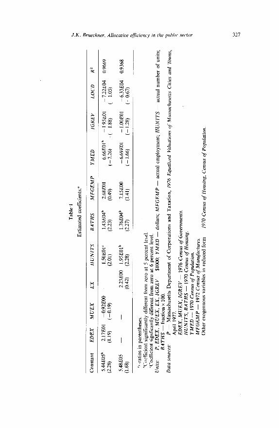
The first line of table 1 shows the TSLS regression results using EDEX, MUEX, HUNITS, BATHS, MFGEMP, YMED, IGREK and LOCD as right-hand variables. Note that the estimated coefficient of BATHS is significantly positive, indicating that, other things equal, a higher proportion of large houses (houses with more than one bathroom) leads to higher
aggregate property value. Similarly, the significantly positive coefficient of Hb’NfTS indicates that a larger number of housing units (and thus a larger stock of commercial structures) leads, other things equal, to higher aggregate value. The coefficient of MFGEMP is positive but insignificant, showing that the effect on aggregate value of differences in stocks of manufacturing structures is too weak to manifest itself in the regressions. The coefficient of the location dummy LOCD has the anticipated negative sign, although the effect of accessibility on aggregate value is apparently not strong enough to yield an estimate significantly different from zero. YMED’s coefficient is significantly negative, indicating that, other things equal, higher incomes reduce property values. A possible explanation for this somewhat surprising result is suggested by the negative correlation in the sample between median
Massachusetts is small enough so that the informational preconditions for arbitrage leading to uniform utilities are present. This argument ignores, however, possible short-run frictions due to job immobility among metropolitan areas, an impediment to mobility which does not arise when all employment is in the central city of one metropolitan area and selection of a community simply involves a choice of residential location.
A related point concerns income variation across municipalities. If utilities for individuals with identical job skills are equalized across cities by income (as well as house price) variation, then it will no longer be true that all people with the same income reach the same utility level. People with identical skills will enjoy equal utilities, but income equality for consumers in different cities could mask a utility differential. This possibility means that control for basic skill characteristics would be necessary to correctly implement the model (community labor force characteristics as well as income levels would appear in the modified regression). On the belief that income variation across the sample cities within skill classes is likely to be relatively unimportant, this modification was not pursued. Note that the above difhculty would not arise if all sample communities belonged to the same labor market.
Tab
le
‘1
Est
imat
ed
coef
licie
nts.
a 2 &
Con
stan
t E
DE
X
MV
EX
E
X
HV
NIT
S B
AT
HS
MFG
EM
P
2 Y
ME
D
IGR
EV
L
OC
D
R2
2 3”
5.44
E05
b 2.
17E
Ol
-0.9
2EO
O
- 1.
50E
Ol’
1.
43E
tIkl
b 2.
68E
Ol
~ 6.
66E
Ol
b -
1.95
EO
l -
7.22
E04
0.
9669
B
(2
.28)
(1
.19)
(-
0.19
) (2
.01)
(2
.23)
(0
.49)
( -
2.
26)
(-1.
88)
(~
1.05
) b z
5.48
E05
-
:: 2.
23E
OO
1.
95E
Ol”
1.
76E
04”
7.15
EO
O
- 6.
69E
Ol
- l.O
OE
Ol
- 6.
3360
4 0.
9368
8.
(1
.68)
(0
.42)
(2
.28)
(2
.27)
(1
.41)
(-
1.
66)
(-
1.28
) (-
0.67
) w
$ “r
-rat
ios
in p
aren
thes
es.
hCoc
flic
ient
si
gniti
cant
ly
diff
eren
t fr
om
zero
at
5
perc
ent
leve
l. 6’
2
‘Coe
tlici
ent
sign
fica
ntly
di
ffer
ent
from
ze
ro
at
6 pe
rcen
t le
vel.
k
Uni
ts:
I’,
ED
EX
, M
VE
X,
EX
, IG
RE
V-
$100
0;
YM
ED
-
dolla
rs;
MFG
EM
P
- ac
tual
em
ploy
men
t; H
VN
ITS
- ac
tual
nu
mbe
r of
uni
ts;
5 ; B
AT
HS
- fr
actio
n x
100.
m
Dat
a so
urce
s:
P ~
M
assa
chus
etts
D
epar
tmen
t of
C
orpo
ratio
ns
and
Tax
atio
n,
1976
E
qual
ized
V
alua
tion
s of
Mas
sach
uset
ts
Cit
ies
and
Tow
ns,
5 A
pril
1977
. E
DE
X,
MU
EX
, IG
RE
V
- 19
76 C
ensu
s of
Gov
ernm
ents
. 6’
HI/
NIT
S,
BA
TH
S -
1970
Cen
sus
of H
ousi
ng.
2 f Y
ME
D
- 19
70 C
ensu
s of
Pop
ulat
ion.
s
MFG
EM
P
- 19
72 C
ensu
s of
Man
ufac
ture
s.
Oth
er
exog
enuo
us
vari
able
s in
red
uced
fo
rm
~ 19
70
Cen
sus
of H
ousi
ng,
Cen
sus
of P
opul
atio
n.
328 J.K. Brueckner, Allocative efficiency in the public sector
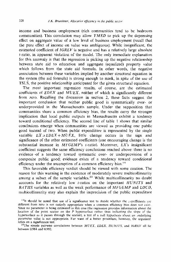
income and business employment (rich communities tend to be bedroom communities). This correlation may allow YMED to pick up the depressing effect on aggregate value of a low level of business employment (recall that the pure effect of income on value was ambiguous). While insignificant, the estimated coefficient of ZGREV is negative and has a relatively large absolute t-ratio, in apparent violation of the model. The only immediate explanation for this anomaly is that the regression is picking up the negative relationship between state aid to education and aggregate (equalized) property value which follows from the state aid formula. In other words, the negative
association between these variables implied by another structural equation in the system (the aid formula) is strong enough to mask, in spite of the use of TSLS, the positive relationship anticipated for the given structural equation.
The most important regression results, of course, are the estimated coefficients of EDEX and MUEX, neither of which is significantly different from zero. Recalling the discussion in section 2, these facts suggest the important conclusion that neither public good is systematically over- or underprovided in the Massachusetts sample. Under the supposition that communities share a common efficiency bias, the results carry the stronger implication that local public outputs in Massachusetts exhibit a tendency toward conditional efficiency. The second line of table 1 shows that similar conclusions emerge when communities are viewed as providing one public good instead of two. When public expenditure is represented by the single variable EX= EDEX+ MUEX, little change occurs in the sign and significance of the other estimated coefficients (one encouraging change is the
substantial increase in MFGEMP’s t-ratio). Moreover, EX’s insignificant coefficient suggests the same efficiency conclusions reached above: there is no evidence *of a tendency toward systematic over- or underprovision of a composite public good; evidence exists of a tendency toward conditional efficiency under the assumption of a common efficiency bias.”
This favorable efficiency verdict should be viewed with some caution. The reason for this warning is the existence of moderately severe multicollinearity
among a subset of the sample variables. ” While multicollinearity no doubt
accounts for the relatively low t-ratios on the important HUNITS and BATHS variables as well as the weak performance of MFGEMP and LOCD, multicollinearity may also explain the imprecision of the public expenditure
“It should be noted that use of ‘a significance test to decide whether the z-coefficients are different from zero is not entirely appropriate when a common effkiency bias does not exist. Since no parameter is being estimated in this case (the regression provides information about the location of the poinl scatter on the P hypersurface rather than indicating the slope of the hypersurface as it passes through the scatter), a test of a null hypothesis about an underlying parameter value is not appropriate. For want of a better procedure, however, the argument relies on a significance test.
“The simple pairwise correlations between MUEX, EDEX, HUNITS, and IGREV all lie between 0.984 and 0.992.
J.K. Brueckner, Allocatioe efjiciency in the public sector 329
coefficients, whose low t-ratios lie behind the favorable efficiency verdict.
Unfortunately, since no remedy exists for the multicollinearity problem, there is no way of evaluating the extent of its influence on the regression results.
It is interesting to compare the present conclusions with those of Brueckner (1979). Using the assumption of a common efficiency bias to interpret a median-value regression, Brueckner concluded that public goods in the well-known Oates (1969) sample were overprovided. The present efficiency verdict, which follows from a much simpler chain of reasoning, is considerably more reliable in spite of the multicollinearity problem discussed
above.
5. Conclusion
The results in this paper suggest that Massachusetts communities exhibit no systematic tendency to over- or underprovide public goods. This means that a representative community is as likely to provide each public good above the level which is Pareto-efficient conditional on its stock of structures as it is to provide it below the conditionally efficient level. If the strong assumption that communities share a common efficiency bias is satisfied, the results suggest the stronger conclusion that the local public sector in Massachusetts exhibits a tendency toward conditional Pareto-efficiency. While similarity of governmental structures among communities in the sample suggests that a common efficiency bias may well exist, the assumption unfortunately remains in the realm of conjecture.
Although the above empirical results are informative and interesting, the paper’s most important contribution is its demonstration that the public sector efficiency question can be addressed empirically using a unified, rigorous framework built on relatively weak assumptions. The other major efficiency study by Barlow (1970) does not share the latter feature since it invokes the median voter model and imposes strong assumptions on functional forms.
As a final observation, it should be realized that the passage in 1980 of Proposition 2 l/2, whose intent was to slash property tax levies in Massachusetts, appears puzzling in light of the present evidence. Apparently, a substantial majority of Massachusetts taxpayers desired a reduction in local public spending, suggesting that public outputs were generally above
Pareto-efficient levels. Of course, voters may have subscribed to the common ‘tax revolt’ notion that reduced government waste would allow maintenance of public consumption levels in the face of smaller budgets. To the extent that this notion was widely held, the passage of Proposition 2 l/2 is not inconsistent with this paper’s empirical conclusions.
330
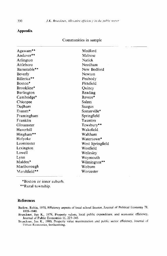
Appendix
Communities in sample
Agawam** Andover** Arlington Attleboro Barnstable** Beverly Billerica** Boston* Brookline* Burlington Cambridge* Chicopee Dedham Everett* Framingham Franklin Gloucester Haverhill Hingham** Holyoke Leominster Lexington
Lowell Lynn Maiden* Marlborough
Marshfield**
Medford Melrose Natick
Needham New Bedford
Newton Peabody Pittsfield Quincy Reading Revere* Salem Saugus Somerville* Springfield Taunton Tewsbury** Wakefield Waltham Watertown* West Springfield
Westfield Wellesley Weymouth Wilmington** Woburn Worcester
*Boston or inner suburb.
**Rural township.
References
Barlow, Robin, 1970, Efficiency aspects of local school finance, Journal of Political Economy 78, 1028-1040.
Brueckner, Jan K., 1979, Property values, local public expenditure, and economic efficiency, Journal of Public Economics 11, 223-245.
Brueckner, Jan K., 1980, Property value maximization and public sector efficiency, Journal of llrhan Economics, forthcoming.
J.K. Bruecknrr, A/locative @cimcy in tkc public sector 331
Eberts, Randall W. and Timothy J. Gronberg, 1981, Jurisdictional homogeneity and the Tiebout hypothesis, Journal of Urban Economics 10, 227-239.
Edel,. Matthew and Eliot Sclar, 1974, Taxes, spending and property values: Supply adjustment in a Tiebout-Oates model, Journal of Political Economy 82, 941-954.
Hamilton, Bruce, 1976, The effects of property taxes and local public spending on property values: A theoretical comment, Journal of Political Economy 84, 647-650.
Oates, Wallace, 1969, The effects of property taxes and local public spending on property values: An empirical study of tax capitalization and the Tiebout hypothesis, Journal of Political Economy 17,957-971.
Pack, Howard and Janet Pack, 1978, Metropolitan fragmentation and local public expenditure, National Tax Journal 31, 349-362.
Samuelson, Paul A., 1954, The pure theory of public expenditures, Review of Economics and Statistics 36, 387-389.
Sonstelie, Jon and Paul Portney, 1978, Profit maximizing communities and the theory of local public expenditure, Journal of Urban Economics 5, 263-277.
Stiglitz, Joseph E., 1977, The theory of local public goods, in: M. Feldstein and R. Inman, eds., Economics of public services (Macmillan. New York) 274-333.
Tiebout, Charles,-1956, A pure iheory of local expenditures, Journal of Political Economy 64, 416-424.