A Systematic Relationship between the Representations of ConvectivelyCoupled Equatorial Wave Activity and the Madden–Julian Oscillation in

Climate Model Simulations

YANJUAN GUO

Joint Institute for Regional Earth System Science and Engineering, University of California, Los Angeles,

Los Angeles, California

DUANE E. WALISER

Joint Institute for Regional Earth System Science and Engineering, University of California, Los Angeles, Los Angeles,

and Jet Propulsion Laboratory, California Institute of Technology, Pasadena, California

XIANAN JIANG

Joint Institute for Regional Earth System Science and Engineering, University of California, Los Angeles,

Los Angeles, California

(Manuscript received 10 July 2014, in final form 20 November 2014)

ABSTRACT

The relationship between a model’s performance in simulating the Madden–Julian oscillation (MJO) and

convectively coupled equatorial wave (CCEW) activity during wintertime is examined by analyzing pre-

cipitation from 26 general circulation models (GCMs) participating in the MJO Task Force/Global Energy

and Water Cycle Experiment (GEWEX) Atmospheric System Study (GASS) MJO model intercomparison

project as well as observations based on the Tropical Rainfall Measuring Mission (TRMM). A model’s

performance in simulating theMJO is determined by how faithfully it reproduces the eastward propagation of

the large-scale intraseasonal variability (ISV) compared to TRMMobservations. Results suggest that models

that simulate a betterMJO tend to 1) have higher fractional variances for various high-frequency wavemodes

(Kelvin, mixed Rossby–gravity, and westward and eastward inertio-gravity waves), which are defined by the

ratios ofwave variances of specific wavemodes to the ‘‘total’’ variance, and 2) exhibit stronger CCEWvariances

in associationwith the eastward-propagating ISVprecipitation anomalies for these high-frequencywavemodes.

The former result is illustrative of an alleviation in the good MJO models of the widely reported GCM de-

ficiency in simulating the correct distribution of variance in tropical convection [i.e., typically too weak (strong)

variance in the high- (low-) frequency spectrum of the precipitation]. The latter suggests better coherence and

stronger interactions between these aforementioned high-frequency CCEWs and the ISV envelope in good

MJO models. Both factors likely contribute to the improved simulation of the MJO in a GCM.

1. Introduction

Tropical convection is known to be organized over

a wide range of spatial and temporal scales, from me-

soscale convective systems (Houze 2004) to convectively

coupled equatorial waves (CCEWs; Kiladis et al. 2009)

and to the planetary-scale Madden–Julian oscillation

(MJO; Madden and Julian 1971, 1972). In this study, we

will focus on the latter two categories that are explicitly

resolved by general circulation models (GCMs).

TheMJO is the dominantmodeof tropical intraseasonal

(30–90 day) variability (ISV), which is characterized by

planetary-scale (;104km), slowly eastward-propagating

(;5ms21) convection anomalies that prevail over the

equatorial Indian Ocean and western Pacific Ocean (e.g.,

Zhang 2005; Wang 2005). The CCEWs include Kelvin,

equatorial Rossby (ER), mixed Rossby–gravity (MRG),

eastward inertio-gravity (EIG), and westward inertio-

gravity (WIG) waves (Takayabu 1994; Wheeler and

Corresponding author address:Dr. YanjuanGuo, Jet Propulsion

Laboratory, M/S 233-304, 4800 Oak Grove Dr., Pasadena, CA

91109.

E-mail: yguo@jifresse.ucla.edu

1 MARCH 2015 GUO ET AL . 1881

DOI: 10.1175/JCLI-D-14-00485.1

� 2015 American Meteorological Society

Kiladis 1999, hereafterWK99; Kiladis et al. 2009), which

correspond to the solutions of the shallow water model

(Matsuno 1966) with a modified equivalent depth

(WK99). The CCEWs can move eastward or westward,

either along the equator or within a few degrees of lat-

itude parallel to it. Among them, Kelvin, MRG, EIG

and WIG waves have typical period of days and spatial

scales of 103 km and, thus, are referred to as tropical

synoptic waves in some literatures (e.g., Khouider et al.

2012). The ER waves are relatively slower and have

comparable temporal and spatial scales compared to the

MJO (WK99; Kiladis et al. 2009). The MJO and the

CCEWs strongly affect the tropical weather and climate,

which has been documented in a large number of pre-

vious studies (e.g., Lau and Waliser 2005; Zhang 2005;

Wang 2005; WK99; Kiladis et al. 2009). In addition, they

influence the midlatitude through various tropical–

extratropical teleconnection patterns. Moreover, the

MJO has been believed to be a key source of untapped

predictability for the extended-range forecast in both

the tropics and the extratropics (e.g., Schubert et al.

2002; Waliser et al. 2003; review in Waliser 2011). Be-

cause of this apparent importance, numerous studies

have been carried out that examine different perspec-

tives of the MJO and CCEW relationship. This study

will focus on exploring possible relationships between

the simulated MJO and CCEWs in climate models.

The MJO and the CCEWs are closely related to each

other within the context of multiscale interaction. The

pioneering work by Nakazawa (1988) using satellite

observations showed that the MJO is a slowly eastward-

propagating, planetary-scale envelope of embedded

eastward-propagating convectively coupled Kelvin

waves, which in turn appear as envelopes of westward-

propagating 2-day waves (orWIG waves). The presence

of the Kelvin wave as well as other types of CCEWs

within the MJO convection complex was identified in

many subsequent studies (Straub and Kiladis 2003;

Haertel and Kiladis 2004; Moncrieff 2004; Kikuchi and

Wang 2010; Zuluaga andHouze 2013). On one hand, the

MJO exerts strong modulation on the CCEWs that form

within it, primarily through its influence on the envi-

ronmental moisture and circulation fields (Roundy and

Frank 2004; Yang et al. 2007; Roundy 2008; Khouider and

Majda 2008b; Khouider et al. 2012; Guo et al. 2014). On

the other hand, the CCEWs feed back to the MJO

through the upscale transports of momentum, tempera-

ture, and moisture (Hendon and Liebmann 1994; Houze

et al. 2000; Moncrieff 2004; Masunaga et al. 2006; Wang

and Liu 2011; Liu and Wang 2012). These two-way in-

teractions between the MJO and the CCEWs are re-

garded as one of the fundamental features of the MJO,

and form the basis of the so-called multiscale models that

had been developed to study the roles of the scale in-

teraction in the MJO (Majda and Klein 2003; Majda and

Biello 2004; Biello andMajda 2005;Majda and Stechmann

2009; Wang and Liu 2011; Liu and Wang 2012).

Despite the attempts of many theoretical and simpli-

fied modeling studies to explain the physics behind the

MJO as well as its multiscale interactions with the

CCEWs, the simulation of the MJO and CCEWs in

GCMs has proven to be a difficult task for decades

(Slingo et al. 1996; Waliser et al. 2003; Lin et al. 2006;

Zhang et al. 2006; Sperber and Annamalai 2008; Yang

et al. 2009; Kim et al. 2009; Straub et al. 2010; Kim et al.

2011; Weaver et al. 2011; Sperber et al. 2008; Huang

et al. 2013; Hung et al. 2013). For example, Slingo et al.

(1996) examined models that were included in the At-

mospheric Model Intercomparison Project (AMIP) and

found that none of the models captured the dominance

of the MJO in space–time spectral analysis identified in

the observations. Lin et al. (2006) examined 14 GCMs

that were included in phase 3 of the Coupled Model

Intercomparison Project (CMIP3), and found that only

two models in CMIP3 have MJO variance comparable

to that observed, and even those two lack realism in

many other MJO features. In terms of the CCEWs, only

about half of the 14 CMIP3 GCMs examined by Lin

et al. (2006) have prominent signals of CCEWs, and the

variances of the simulated CCEWs, except the eastward

inertio-gravity and Kelvin waves, are generally weaker

compared to the observations. Yang et al. (2009) also

showed that the simulated CCEWs in theHadley Centre

climate models are deficient. Straub et al. (2010) further

investigated the CCEWs in 20 CMIP3 coupled GCMs,

and found that only a fewmodels can simulate the Kelvin

wave with a realistic activity distribution and spatial

structure. As an update to the study by Lin et al. (2006),

Hung et al. (2013) examined 20 models from phase 5 of

CMIP (CMIP5) and found that CMIP5 models gener-

ally produce larger variances of MJO, Kelvin, ER, and

EIG waves compared to those in CMIP3. But there are

still very few models that are able to simulate realistic

eastward propagation of the MJO. Challenges for

faithfully simulating the MJO and the CCEWs are re-

lated to model issues concerning the convective pa-

rameterization [see a brief summary in the introduction

of Hung et al. (2013)], boundary layer parameteriza-

tion, cloud microphysics, etc.

As efforts toward improving the MJO performance in

GCMs are continuously required, theWorkingGroup on

Numerical Experimentation (WGNE) MJO Task Force

(MJOTF) and Global Energy and Water Cycle Experi-

ment (GEWEX) Atmospheric System Study (GASS)

have recently combined forces under the auspices ofYear

of Tropical Convection (YOTC; Moncrieff et al. 2012;

1882 JOURNAL OF CL IMATE VOLUME 28

Waliser et al. 2012) to organize a model intercomparison

project to improve our understanding of the MJO (the

MJOTF/GASS project), particularly focusing on the es-

sential roles and vertical structure of diabatic heating and

related moist processes in MJO physics (Petch et al.

2011). This MJO model intercomparison project consists

of three experimental components, including (i) a 20-yr

climate simulation, (ii) a 20-day hindcast, and (iii) a 2-day

hindcast component. Comprehensive results based on

each component are being first reported in three research

papers, respectively (Jiang et al. 2015; Xavier et al. 2015;

Klingaman et al. 2015).

In this study, we will make use of the outputs from 26

models that contributed to the 20-yr climate simulation

component of this project. Precipitation data over the

20-yr period are used to examine the general behavior of

the MJO and the CCEW activity in the model simula-

tions. Our focus will be on exploring the possible re-

lationships between a model’s performance in simulating

the MJO and its simulation of the CCEW activity across

a large number of GCM simulations, which has not been

examined before. Previous multimodel studies usually

evaluated the performance of the MJO and the CCEWs

separately, with little emphasis on the linkage between

these two. One possible reason is that most GCMs are

unable to simulate a realistic MJO (Lin et al. 2006; Hung

et al. 2013), so there is a lack of basis to further examine

its relationship to the higher-frequency CCEWs. How-

ever, as will be shown in this study, about a quarter of the

models that participated in the MJOTF/GASS project

show reasonable simulations of the MJO, making the

current study feasible.

The rest of this paper is organized as follows. Section 2

describes the data and methodology used in this paper,

including the identification of the ISV (as a measure of

the MJO) and the CCEWs, and the approach to scoring

a model’s MJO performance. Section 3 discusses the cli-

matology of the ISV and CCEW activity, as well as pos-

sible relationships between the strength of the CCEW

variance and theMJOperformance across all themodels.

In section 4, we will examine the variations of the CCEW

activity associated with the ISV variation, and the im-

plication of this CCEW–ISV interaction for the MJO

simulation. Finally, discussions and conclusions are pre-

sented in section 5.

2. Data and methodology

a. Data

In this study, precipitation, which is indicative of the

large-scale convective signal, is the only meteorological

variable used. Precipitation data are examined for both

GCM simulations and observation.

Table 1 lists the 26 models examined in this study that

participated in the MJOTF/GASS MJO model inter-

comparison project. These model simulations are either

with an atmosphere-only GCM (AGCM) or based on an

atmosphere–ocean coupled system (denoted by an as-

terisk). More details can be found at the project website

(http://www.ucar.edu/yotc/mjodiab.html). Twenty-year

daily precipitation data during 1991–2010 from each

model have been regridded onto a common 2.58 3 2.58latitude–longitude grid.

Observations of precipitation taken from the Tropical

Rainfall Measuring Mission (TRMM) 3B42 version 7

dataset (Huffman et al. 2007) that have been interpolated

onto the same temporal and horizontal resolution as the

model simulations, are used to compare with the model

outputs. The time period of the TRMMdata is from 1998

to 2012.

This study focuses on the Northern Hemisphere ex-

tended winter season (November–April) when the tra-

ditionally defined MJO is most active and coincident

with the near-equatorial region (e.g., Waliser 2006).

b. WK-filtering method for extracting CCEWanomalies

To isolate the convection signals corresponding to the

CCEWs, a zonal wavenumber–frequency filtering, or so-

calledWKfiltering (WK99), is applied to the precipitation

data. This is accomplished by retaining only those spectral

coefficients corresponding to the spectral peaks associ-

ated with a specific mode in the wavenumber–frequency

domain. The domains used to extract individual CCEWs

are indicated in Table 2, which follow those defined by

Kiladis et al. (2009). More details on the WK-filtering

method can be found in WK99. Both symmetric and

asymmetric components about the equator are retained

for these CCEWs.

Prior to the WK filtering, the annual cycle (mean

and the first three harmonics) of the precipitation was

first removed from its daily time series to produce the

anomalies at each grid point. These anomalies are called

the total anomalies in this study since variability on all

time scales is retained except for the annual cycle. These

total anomalies are then used to carry out the WK fil-

tering to produce the individual CCEWwave anomalies,

namely ER, Kelvin, MRG, andWIG and EIG waves. In

addition, a 20–100-day bandpass filtering is applied to

obtain the ISV anomalies, which are used in this study to

generally represent the model’s MJO variability and, in

particular, to provide a means of scoring the model’s

MJO performance (described later in section 2d). The

winter variances of the individual wave modes based on

TRMMprecipitation data are shown in Fig. 1 to provide

the climatological maps of the wave activity of these

1 MARCH 2015 GUO ET AL . 1883

waves from the observational perspective. It can be seen

that the observed precipitation variances are largely

confined to the Indian Ocean and western Pacific warm

pool region between 158S and 158N, and this will be our

region of interest.

c. Linear regression analysis

In this study, the linear regression technique is

heavily used; thus, it is briefly described here. Assume

that there are n data points for the dependent variable y

and the explanatory variable x. The goal of the linear

regression is to find a straight line that best fits the data

points. With the least squares approach, the slope of the

fitted line (b) is determined as the correlation between y

and x corrected by the ratio of the standard deviations of

y and x:

b5 rxy

sy

sx, (1)

in which rxy is the correlation between y and x and sy and

sx are the standard deviations of y and x, respectively.

The slope b can be interpreted as the conditionally ex-

pected change in y for a one-unit change in x, which is

the quantity that will be examined later on.

TABLE 1. Participatingmodels with horizontal and vertical resolutions andmain references. CoupledGCMmodels are denoted with an

asterisk. Spectral model horizontal resolutions are listed with their spectral wavenumber truncations (preceded by T for triangular and R

for rhomboidal) and the associated Gaussian grid spacing in parentheses. [Adopted from Table 1 in Jiang et al. (2015).]

Model name Institution

Horizontal resolution,

vertical levels Reference

1 NASAGMAO_GEOS5 NASA Global Model and Assimilation

Office, United States

0.6258 3 0.58, L72 Molod et al. (2012)

2 SPCCSM* George Mason University, United States T42 (2.88), L30 Stan et al. (2010)

3 GISS_ModelE2 NASA Goddard Institute for Space Studies,

United States

2.758 3 2.28, L40 Schmidt et al. (2014)

4 EC_GEM Environment Canada, Canada 1.48, L64 Coté et al. (1998)5 MIROC Japan Agency for Marine–Earth Science and

Technology, Japan

T85 (1.58), L40 Watanabe et al. (2010)

6 MRI-AGCM Meteorological Research Institute, Japan T159, L48 Yukimoto et al. (2012)

7 CWB_GFS Central Weather Bureau, Taiwan T119 (18), L40 Liou et al. (1997)

8 PNU_CFSv1 Pusan National University, South Korea T62 (28), L64 Saha et al. (2006)

9 MPI_ECHAM6* Max Planck Institute for Meteorology,

Germany

T63 (28), L47 Stevens et al. (2013)

10 MetUM_GA3 Met Office, United Kingdom 1.8758 3 1.258, L85 Walters et al. (2011)

11 NCAR_CAM5 National Center for Atmospheric Research,

United States

T42 (2.88), L30 Neale et al. (2012)

12 NRL_NAVGEMv1.0 Naval Research Laboratory, United States T359 (37 km), L42 Hogan et al. (2014)

13 UCSD_CAM Scripps Institute of Oceanography,

United States

T42 (2.88), L30 Zhang and Mu (2005)

14 NCEP_CFSv2 NOAA/NCEP/Climate Prediction Center,

United States

T126 (18), L64 Saha et al. (2014)

15a CNRM_AM Météo-France/Centre National de laRecherche Scientifique, France

T127 (1.48), L31 Voldoire et al. (2013)

15b CNRM_ACM

15c CNRM_CM

16 CCCma_CanCM4* Canadian Centre for Climate Modelling and

Analysis, Canada

T63 (1.98), L35 Merryfield et al. (2013)

17 BCCAGCM2.1 Beijing Climate Center, China Meteorological

Administration, China

T42 (2.88), L26 Wu et al. (2010)

18 FGOALS-s2 Institute of Atmospheric Physics, Chinese

Academy of Sciences, China

R42 (2.88 3 1.68), L26 Bao et al. (2013)

19 NCHU_ECHAM5* Academia Sinica, National Chung Hsing

University, Taiwan

T63 (28), L31 Tsuang et al. (2001)

20 TAMU_Modi-CAM4 Texas A&M University, United States 2.58 3 1.98, L26 Lappen and Schumacher (2012)

21 ACCESS Centre for Australian Weather and Climate

Research, Australia

1.8758 3 1.258, L85 Zhu et al. (2013)

22 ISUGCM Iowa State University, United States T42 (2.88), L18 Wu and Deng (2013)

23 LLNL_CAM5ZMMicro Lawrence Livermore National Laboratory,

United States

T42 (2.88), L30 Song and Zhang (2011)

24 SMHI_ecearth3 Rossby Centre, Swedish Meteorological and

Hydrological Institute, Sweden

T255 (80 km), L91 Hazeleger et al. (2012)

1884 JOURNAL OF CL IMATE VOLUME 28

In this study, the ISV anomaly is the explanatory

variable x, and a time series of ISV anomalies work as an

ISV index onto which other quantities (y) are regressed.

d. Determination of the MJO performance of a GCM

In this study, a GCM’sMJO performance is evaluated

according to its ability in capturing the key characteris-

tics of the MJO, the coherent large-scale eastward

propagation of the ISV anomalies, which is revealed by

the lag regression of the ISV anomalies against an ISV

index at a reference point following the approach used

by Jiang et al. (2015). To be specific, the daily time series

of the equatorially averaged (108S–108N for Kelvin,

MRG, WIG, and EIG waves; 158S–158N for ER waves)

ISV anomalies during the multiyear period (winter sea-

son only) were regressed against an ISV index, which is

defined as the ISV anomalies averaged over a small ref-

erence box. For example, 58S–58N, 758–858E is used for the

Indian Ocean reference point. The regression was done at

time lags fromday220 to day 20 to generate aHovmöller-like diagram (Fig. 2). The systematic eastward propaga-

tion of precipitation associated with the observed MJO

starting from the Indian Ocean and dissipating near the

date line is clearly seen based on TRMM data (Fig. 2,

top left panels outlined by a rectangle).

Note that in the above lag-regression procedure, we

purposely used the ISV anomalies (thus the ISV index)

instead of theMJO anomalies (and a formalMJO index)

to avoid preconditioning the answer by only examining/

extracting the large-scale eastward-propagating part of

the ISV. The underlying argument is that the systematic

eastward propagation of the ISV will emerge in the lag

regression of the ISV plot in the observations as well as

in theGCMs with reasonableMJO simulations since the

MJO dominates the ISV in the real atmosphere. On the

other hand, in models with a poor depiction of theMJO,

which often means that the model simulates too strong

westward-propagating features, examining the ISV

anomalies rather than the MJO anomalies will not pre-

maturely exclude these features, thus providing the

means to discern the true quality of the GCMs’ repre-

sentation of the MJO.

It is found that about one-quarter of the models can

capture this eastward-propagatingMJOmode quite well

(NCHU_ECHAM5-SIT, TAMU_modCAM4, GISS_

ModelE2, CNRM_CM, SPCCSM, PNU_CFS, and MRI_

AGCM; seeFig. 2), and a fewmore are able to simulate the

eastward propagation to a lesser degree (SMHI_ecearth3,

CNRM_ACM, FGOALS-s2, LLNL_CAM5ZMMicro,

and MPI_ECHAM6). Finally, more than half of the

models show stationary or even westward-propagating

signals, and the anomalies are confined to a much

smaller zonal extent than that observed, indicating that

TABLE2.N

amesofindividualw

avemodes(firstrow),thefilteringmethodsusedto

extractthem

(secondrow),andnumberofGCM

modelswithwavevariance

smallerthantheTRMM

observationsforeach

ofthem

(thirdrow).Forthewavenumberkshown,apositivesigndenoteseastward

propagation,whileanegativesign

isforwestward

propagation.heisthe

‘‘equivalentdepth.’’

Wave

mode

Total

ISV

ER

Kelvin

MRG

WIG

EIG

Filtering

method

Rem

ovalofthe

firstthree

harm

onicsof

theseasonalcycle

20–100day

30–96

day;

210,

k,

21;

dispersioncurves

withheof8and100m

2.5–14day;

1,

k,

14;

dispersioncurves

withheof8and50m

27,

k,

21;

dispersioncurves

withheof12and50m

210,

k,

21;

dispersion

curveswith

heof25and50m

1,

k,

14;

dispersioncurves

withheof25and50m

No.of

models

withweaker

thanobserved

variance

19

16

14

22

21

25

24

1 MARCH 2015 GUO ET AL . 1885

realistic simulation of the MJO is still a highly chal-

lenging issue. Nevertheless, compared to CMIP3 (Lin

et al. 2006) and CMIP5 (Hung et al. 2013) ensembles,

there are relatively more models that show reasonably

good MJO simulation in the MJOTF/GASS project.

One reason might be that some models have imple-

mented specific strategies to help improve the model’s

MJO simulation, as that is the core target of this pro-

ject. For example, SPCCSM implemented the ‘‘super-

parameterization’’ technique, which has been reported

to lead tomuch improvedMJO simulations (e.g., Benedict

and Randall 2007). In TAMU_modCAM4, the ‘‘ob-

served’’ vertical latent heating profile based on TRMM

estimates was assimilated in order to accurately depict

both the horizontal and vertical distributions of heating

throughout the tropics, which was shown to help im-

prove the MJO simulation significantly (Lappen and

Schumacher 2012). More detailed discussions regard-

ing the configurations of the participating models can

be found in Jiang et al. (2015).

FIG. 1. Geographical distribution of boreal winter (December–April) mean variances of

(top)–(bottom) the total, ISV, ER, Kelvin, MRG, WIG, and EIG wave modes based on the

TRMM observations during 1998–2012 (mm2 day22). The red box encompasses from the

Indian Ocean to the western Pacific Ocean region. (regional mean variances computed over

this region are shown in Figs. 3b–e).

1886 JOURNAL OF CL IMATE VOLUME 28

FIG. 2. Lag–longitude diagram of 108S–108N-averaged ISV (20–100-day filtered) precipitation anomalies (mmday21) regressed against

the IndianOcean ISV index, which is defined as the 20–100-day filtered precipitation anomalies averaged over 58S–58N, 758E-858E, at a lagtime from day220 to day 20; values correspond to 1mmday21 ISV precipitation anomaly Pattern correlation between the panel for each

model and that for TRMM observations is used to determine theMJO score for this model (see Fig. 3a) when combined with the western

Pacific case. Except for TRMM, good composite, and bad composite panels outlined by a rectangle in the top left, the individual models are

shown indescending order of theirMJOscoresmoving down thefigure from left to right. The goodMJOcomposite (indicated by a large green

dot) is based on the average of the seven bestMJOmodels (indicated by a small green dot in top right of the panels), while the bad composite

(indicated by a large red dot) is the average of the seven worst MJO models (indicated by a small red dot in top right of the panels).

1 MARCH 2015 GUO ET AL . 1887

The pattern correlation between the Hovmöller dia-gram computed from each model simulation and thatbased on the TRMM observations is then calculatedover the domain of 508E–1808 and from day 220 to day

20 to evaluate how well the eastward-propagation pat-

tern in that model resembles the observations. Then, the

same procedure is applied to calculate another set of

spatial correlation coefficients except that a reference

box in the western Pacific (58S–58N, 1308–1508E) is usedwhen conducting lag-regression analyses. The resulting

patterns are very similar to those for the Indian Ocean

case for all the models. The Pacific patterns are not

shown here, but can be found in Fig. 4 of Jiang et al.

(2015). Combining the coefficients based on both the

Indian Ocean and the western Pacific cases, an MJO

score can be finally assigned to each model simulation,

which is shown in Table 3.

Results from the seven models (about one-quarter of

total number of models) with the highestMJO scores are

then composited to form the ‘‘good’’ MJO composite,

and those from the seven models with the lowest MJO

scores form the ‘‘bad’’ MJO composite. From Table 3, it

can be seen that good MJO models have MJO scores

larger than 0.85, while bad models have scores smaller

than 0.65. The good composite again shows an eastward

propagation close to the observations, while the bad

composite displays a slight westward-propagation signal

with a much smaller horizontal scale than is exhibited by

the observed MJO (Fig. 2).

3. Climatology of ISV and CCEW activity

Before we proceed to explore the multiscale structure

of the MJO, the climatology of the ISV and the CCEW

activity is first examined in this section. The precipitation

variances are first computed for the ISV and CCEWs, as

well as the total wave mode over the entire tropics. Note

that only winter seasons are used. The variances based on

the TRMM observations have been shown in Fig. 1. For

brevity, the counterparts of the 26 GCM simulations

based on 20 winters (1991–2010) are not shown.

A regional mean of the wave variance is further

obtained by averaging the variances at all grid points

over the Indo-Pacific warm pool region (158S–158N,

508E–1808; see the red box in the top panel of Fig. 1),

which is the region with MJO activity. Note that there is

also strong CCEW activity outside of the Indo–western

Pacific region such as over South America and the

tropical Atlantic Ocean.We chose to average the CCEW

activity over the MJO-active region instead of the entire

tropics as our focus is on the interaction between the

CCEWs and the MJO. Nevertheless, we have performed

exactly the same calculations except averaging over the

entire tropics (158S–158N, all longitudes), and the results

lead to the same conclusion.

a. Strength of ISV and CCEW activity

The precipitation variances averaged over the Indo-

Pacific warm pool region for each wave based on the 26

GCM simulations and TRMM observations are shown

in Fig. 3. Examination of the climatology of the ISV and

CCEW activity reveals a few interesting features.

First, the climatological wave activity exhibits large

model-to-model variations: for example, for the ISV

(Fig. 3b), the model with the largest variance (from

BCCAGCM21) has variance that is about 4 times that of

the smallest one (from LLNL_CAM5ZMMicro). Such

large model-to-model variations in the amplitude of the

wave variance are present in all wave modes, and can be

traced back to the variation in the total wave variance

(Fig. 3a). Note that the correlations between the ISV

and different wave variances (bars in Figs. 3b–g) and the

total variance (bars in Fig. 3a) among the 26 models and

the TRMM data are all above 0.9. This indicates that

a model with large (small) total precipitation variance

TABLE 3. MJO scores for 26 GCM simulations and TRMM ob-

servations, which are computed following the approach introduced

in section 2d. The seven models (about one-quarter of the total

number ofmodels) with highestMJO scores (boldface) are used for

the good MJO composite, while the seven models with lowest

scores (italics) are used for the bad MJO composite.

Model ID MJO score

TRMM 1.00

NCHU_ECHAM5-SIT 0.92

TAMU-modCAM4 0.92

GISS_ModelE2 0.91

CNRM_CM 0.90

SPCCSM 0.89

MRI_AGCM 0.89

PNU_CFS 0.87

SMHI_ecearth3 0.83

CNRM_ACM 0.81

FGOALS-s2 0.81

LLNL_CAM5ZMMicro 0.80

CNRM_AM 0.77

ACCESS 0.75

MPI_ECHAM6 0.74

NASAGMAO_GEOS5 0.73

NCAR_CAM5 0.72

EC_GEM 0.71

UCSD_CAM 0.68

BCCAGCM21 0.67

MetUM_GA3 0.64

NRL_NAVGEMv.01 0.64ISUGCM 0.61

MIROC5 0.59

CWB_GFS 0.59

NCEPCPC_CFSv2 0.59CCCma_CanCM4 0.59

1888 JOURNAL OF CL IMATE VOLUME 28

tends to also exhibit strong (weak) precipitation vari-

ability associated with the ISV and CCEW modes.

Second, comparison between model simulations and

the TRMM observations (denoted by the leftmost point

and horizontal dotted lines) suggests that a longstanding

problem in GCM simulations of tropical convection still

exists: most of the participating models produce smaller

precipitation variances compared to the observations

FIG. 3. Boreal winter (December–April) mean variances averaged over 158S–158N, 508E–1808 (indicated by the red box in Fig. 1) for 26 GCM models and TRMM observations for

(a) total, (b) ISV, (c) ER, (d) Kelvin, (e) WRG, and (f) WIG and (g) EIG wave modes

(mm2 day22). The period of model simulations is from 1991 to 2010, while for TRMM it is from

1998 to 2012. Dashed lines indicate the TRMM value of each mode. Value in the top-right

corner of each panel indicates the correlation coefficient between the mean variance of each

mode and the MJO score across 26 GCM models and TRMM observations.

1 MARCH 2015 GUO ET AL . 1889

for the ISV and all CCEWmodes, a phenomenonwe call

‘‘weak wave variance’’ bias in this study. Table 2 lists the

number of models that have weaker variance than that

based on TRMM. It can be seen that 14 out of 26 models

produce variance that is weaker than that found in

TRMM for the ER mode, and 16 out of 26 for the ISV

mode. Even worse, more than 20 models display the

weak variance bias for the Kelvin,MRG,WIG, and EIG

modes. Thus, the weak wave variance bias tends to be

more severe for higher-frequency modes than for lower-

frequency modes (ISV and ER).

This weak wave variance bias has already been iden-

tified for the CMIP3 and CMIP5 models (Lin et al. 2006;

Hung et al. 2013). Nevertheless, our results suggest that

models may be exhibiting some improvements in this

aspect: in CMIP3 almost all GCMs show such a bias for

all CCEWs; in CMIP5 this bias is still present for all the

wave modes (except for EIG) in almost all the models,

but the wave variances have been generally increased

compared to their CMIP3 counterparts. Our results in-

dicate that for models participating in theMJOTF/GASS

MJO model intercomparison project, some models pro-

duce larger CCEW variances that those observed.

b. Linkage between the strength of the ISV andCCEW variance and the MJO score

As discussed in section 3a, somemodels display better

simulations of the strength of CCEWs than others. Given

the fact that the MJO is often characterized as a slowly

eastward-propagating, planetary-scale envelope of em-

bedded CCEWs, one might hypothesize that a model’s

ability in realistically simulating the MJO may impact its

ability to adequately simulate the strength of theCCEWs,

or vice versa. To test this hypothesis, we will examine the

possible linkage between the strength of eachCCEWand

the model’s MJO performance across GCM simulations.

The correlation between the climatological variance

of each wave mode (Figs. 3a–g) and the MJO score

(Table 3) across 26 GCM simulations and TRMM ob-

servation is calculated and denoted by the number at the

top-right corner of each panel in Fig. 3. It can be seen

that there indeed exists some degree of positive corre-

lation between the climatological wave strength and the

MJO performance for the Kelvin, MRG,WIG, and EIG

wave modes. The correlation coefficients range from

0.19 to 0.35 for 27 samples (26models1TRMM), which,

except for theWIGmode, are not significant at the 90%

level based on a two-tailed Student’s t test. Furthermore,

it is noted that the strengths of the ISV and ER, as well

as the total wave activity, display nearly zero correlation

with the MJO score.

It turns out that much stronger correlations between

amodel’sMJO performance and its simulation of Kelvin,

MRG, WIG, and EIG wave activity are revealed when

the absolute wave variances are replaced by the ‘‘frac-

tional variances.’’ Here, fractional variance is defined as

the fraction of a wave mode’s absolute variance relative

to the total wave variance. The relations between the

fractional variance of the ISV and CCEWs and the MJO

score in the 26 GCM simulations plus the TRMM ob-

servation are displayed by scatterplots in Fig. 4. Strong

correlations between the MJO score and the fractional

variances are found for the Kelvin,MRG,WIG, and EIG

wave modes, with correlation coefficients of 0.58, 0.58,

0.51, and 0.49, respectively, all significant at the 99%

confidence level based on a two-tailed Student’s t test.

These statistically significant correlations indicate that

models having better MJO performance tend to simulate

larger Kelvin, MRG,WIG, and EIG fractional variances,

and vice versa (Figs. 4b–e). Recall the weak wave vari-

ance bias that existed inGCM simulations of the CCEWs

discussed above, which is especially severe for high-

frequency modes such as Kelvin, MRG, WIG, and EIG

waves (Table 2). Thus, larger fractional variances of these

modes mean that the weak variance bias is less severe in

these models (Figs. 4b–e), which is likely also related to

the improvement of the model’s MJO simulation. This

suggests that when a model has a better MJO, its total

variance is also more coherently organized into CCEW

modes.

Another important CCEW is the ER wave. Figures 4f

and 3c suggest that the strength of the ER mode has no

correlation with themodel’sMJOperformance in terms of

either fractional or absolute variance. Note that compared

to Kelvin, MRG, WIG, and EIG waves, the ER wave is

a relatively larger-scale and lower-frequency mode.

It should also be noted that the strength of the ISV

itself exhibits very weak correlation with the model’s

MJO performance when the fractional variance is used

(0.08; see Fig. 4a). The correlation decreases to about

zero (20.01) when the absolute variance is considered

(Fig. 3c). This is different from what is shown by Kim

et al. (2011), in which a significant positive correlation is

found between the ISV variance and the MJO perfor-

mance. Note that in their study, the MJO performance is

quantified by the ratio of the MJO (wavenumbers 1–3

and 30–60 day) variance to its westward counterpart,

which highly correlates with our MJO score (0.77; Jiang

et al. (2015)) as both methods concern the eastward-

propagating feature of the ISV band. The discrepancy

between our results and those of Kim et al. (2011) in

terms of veryweak or strong positive correlation between

the ISV variance strength and the MJO performance

might be partly due to the fact that their results are based

on a rather limited number of climate models: they ex-

amined 10 simulations from five AGCMs (some have

1890 JOURNAL OF CL IMATE VOLUME 28

FIG. 4. Scatterplots of theMJO score and the fractions of (a) ISV, (b)Kelvin, (c)MRG, (d)WIG, (e) EIG, (f) ER, and (g) low-frequency

(period. 100 day) mode variance relative to the total variance, and (h) the summed Kelvin, MRG, andWIG and EIG variances relative

to the low-frequency mode variance. Filled circles represent individual GCM simulations, while a filled square represents the TRMM

observations. The correlation coefficient of each scatterplot is indicated by the number in the top-right corner of the panel. Correlation

coefficients that are statistically significant at the 90%, 95%, and 99% confidence levels for 27 samples are 0.32, 0.37, and 0.48 respectively,

based on the two-tailed Student’s t test.

1 MARCH 2015 GUO ET AL . 1891

sensitivity experiments by tuning cumulus parameteri-

zation), and furthermore, two of the five models are dif-

ferent versions of the Community Atmosphere Model

(CAM). In this sense, our conclusion is probably more

robust than theirs.

As we have shown above, strong linkage between

a model’s MJO and CCEW performance can only be

found for the Kelvin, MRG, WIG, and EIG wave

modes, with such a linkage being absent for the ER

mode and the ISV. Since the Kelvin, MRG, WIG, and

EIG waves are all located over the high-frequency end

of the precipitation spectrum, it is of interest to examine

the behavior of the precipitation anomalies toward the

other end of the spectrum. Here, we examine the low-

frequency part of the precipitation, defined as pre-

cipitation anomalies with periods longer than 100 days,

which we denote as the .100 day component. The cor-

relation between its fractional variance and the MJO

score is shown in Fig. 4g, which is highly negative

(20.57), indicating that the better a model performs in

simulating the MJO, the smaller is the fractional vari-

ance of its low-frequency band. This is opposite to the

Kelvin,MRG,WIG, and EIG cases. Combining the high-

and low-frequency components together, it is suggested

that a model with better MJO performance tends to have

relatively stronger variance in high-frequency modes and

weaker variance in the low-frequency mode, which is

further clearly revealed in Fig. 4h where a scatterplot of

the ratio of the high-frequency band to the low-frequency

band and the MJO score is shown (the correlation is as

high as 0.72). It should also be noted that in all cases in

Fig. 4, except for the ISV and ER modes, models having

higherMJO scores tend to have fractional variance ratios

that are closer to those observed.

This finding is encouraging in the sense that the increase

in high-frequency precipitation variance and the reduction

in low-frequency precipitation variance correspond to the

alleviation of long-existing problems in GCM simulations.

Previous studies based onCMIP3 andCMIP5models (Lin

et al. 2006; Hung et al. 2013) have found that the simulated

precipitation tends to contain too much variance at the

low-frequency end of the space–time spectrum, which was

referred to as the overreddened spectrum phenomenon.

This phenomenon was also noticed as a tendency for too

much persistent light rain in other studies (Dai 2006;

Boberg et al. 2009). Along with the overestimation of the

low-frequency precipitation variance, Lin et al. (2006) and

Hung et al. (2013) also found that the precipitation vari-

ance at the high-frequency end is significantly under-

estimated, such that the CCEW variance is much weaker

than that observed. Thus, the tendency for increased high-

frequency precipitation variance and decreased low-

frequency precipitation variance occurs in conjunction

with models having better MJO scores corresponds to an

alleviation of the aforementioned model deficiencies in

simulations using these models.

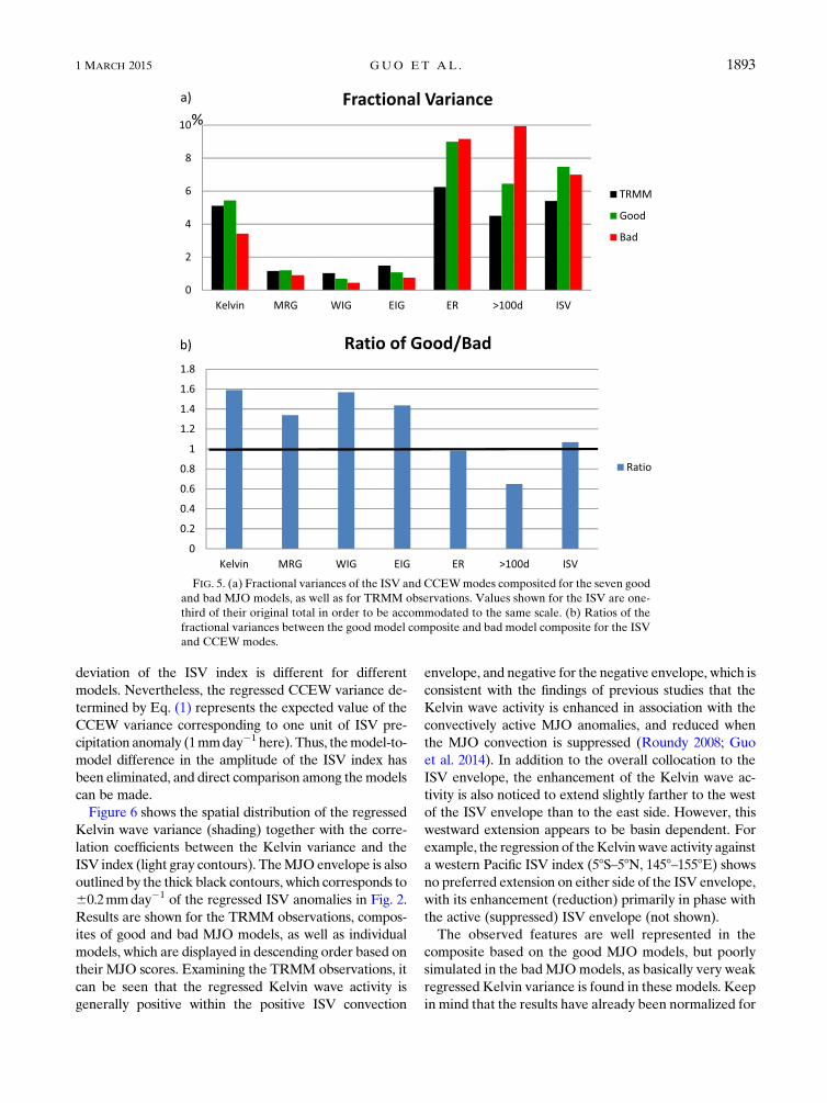
Furthermore, the composite results based on the top

seven good and bottom seven bad MJO models

according to their MJO scores are summarized in Fig. 5.

Again, it can be seen that the fractional variances of

Kelvin, MRG, WIG, and EIG wave modes in the good

models are systematically larger than their counterparts

in the bad models, and closer to the observational re-

sults. The magnitudes of these high-frequency mode

variances in the good model composites are about 1.5

times of those in the bad model composites. At the same

time, the fractional variance of the low-frequency vari-

ability is much smaller in the good model composite

than that in the bad composite and, thus, more consis-

tent with the observational result. It is also noted that

the composite ER and ISV wave variances in both

groups have almost the same magnitude and are both

larger than those observed. Note that ER wave forms

essential part of the ISV mode, thus strongly contrib-

uting to the stronger-than-TRMM ISV variance.

4. Implication of the multiscale interactionbetween CCEW and MJO for the MJOperformance

In the preceding section, we have revealed a strong

linkage between the climatological behavior of the high-

frequency CCEW (Kelvin, MRG,WIG, and EIG waves)

activity and theMJO performance in the climate models.

Here, we will further examine the multiscale interaction

between theCCEWactivity and theMJO in thesemodels

to see if there is any systematic relationship between the

representation of the CCEW–MJO interaction and the

simulation of the MJO.

The linear regression analysis is used here to explore

the multiscale interaction between the CCEWs and the

MJO. To be specific, the time series of the squared

CCEW anomalies during the entire period at each grid

point over the Indo–western Pacific are regressed onto

the Indian Ocean ISV index (20–100-day filtered pre-

cipitation anomalies averaged over 58S–58N and 758–858E). The regression coefficient b at each point can

then be computed using Eq. (1). Here, sx is the standard

deviation of the ISV index, sy is the standard deviation of

the time series of the squaredCCEWanomalies, and rxy is

the correlation between them. Thus, the regression co-

efficient represents the conditionally composited CCEW

variance, and we call it regressed CCEWvariance or ISV-

associatedCCEWvariance in later discussions for brevity.

Note that the strength of the ISV precipitation varies in

different GCM simulations (Fig. 3c); thus, the standard

1892 JOURNAL OF CL IMATE VOLUME 28

deviation of the ISV index is different for different

models. Nevertheless, the regressed CCEW variance de-

termined by Eq. (1) represents the expected value of the

CCEW variance corresponding to one unit of ISV pre-

cipitation anomaly (1mmday21 here). Thus, themodel-to-

model difference in the amplitude of the ISV index has

been eliminated, and direct comparison among themodels

can be made.

Figure 6 shows the spatial distribution of the regressed

Kelvin wave variance (shading) together with the corre-

lation coefficients between the Kelvin variance and the

ISV index (light gray contours). TheMJOenvelope is also

outlined by the thick black contours, which corresponds to

60.2mmday21 of the regressed ISV anomalies in Fig. 2.

Results are shown for the TRMM observations, compos-

ites of good and bad MJO models, as well as individual

models, which are displayed in descending order based on

their MJO scores. Examining the TRMM observations, it

can be seen that the regressed Kelvin wave activity is

generally positive within the positive ISV convection

envelope, and negative for the negative envelope, which is

consistent with the findings of previous studies that the

Kelvin wave activity is enhanced in association with the

convectively active MJO anomalies, and reduced when

the MJO convection is suppressed (Roundy 2008; Guo

et al. 2014). In addition to the overall collocation to the

ISV envelope, the enhancement of the Kelvin wave ac-

tivity is also noticed to extend slightly farther to the west

of the ISV envelope than to the east side. However, this

westward extension appears to be basin dependent. For

example, the regression of theKelvinwave activity against

a western Pacific ISV index (58S–58N, 1458–1558E) showsno preferred extension on either side of the ISV envelope,

with its enhancement (reduction) primarily in phase with

the active (suppressed) ISV envelope (not shown).

The observed features are well represented in the

composite based on the good MJO models, but poorly

simulated in the badMJOmodels, as basically very weak

regressed Kelvin variance is found in these models. Keep

in mind that the results have already been normalized for

FIG. 5. (a) Fractional variances of the ISV and CCEWmodes composited for the seven good

and bad MJO models, as well as for TRMM observations. Values shown for the ISV are one-

third of their original total in order to be accommodated to the same scale. (b) Ratios of the

fractional variances between the good model composite and bad model composite for the ISV

and CCEW modes.

1 MARCH 2015 GUO ET AL . 1893

FIG. 6. Latitude–longitude pattern of the Kelvin wave variance (shading; mmday21) regressed against the Indian Ocean ISV index,

which is defined as the 20–100-day filtered precipitation anomalies averaged over 58S–58N, 758–858E; the values of the Kelvin variance

correspond to 1 ISV precipitation anomaly. Light gray contours are the correlation coefficients between the Kelvin wave variance and the

ISV index. The contour interval is 0.1, and the contour of 0 is omitted. Thick black contours outline the 60.2mmday21 lines of the

regressed ISV anomalies themselves to represent the MJO envelope. The good MJO composite (indicated by a large green dot) comes

from the average of the seven best MJO models (indicated by a small green dot in the top right of the panels), while the bad composite

(indicated by a large red dot) is from the seven worst MJO models (indicated by a small red dot in the top right of the panels).

1894 JOURNAL OF CL IMATE VOLUME 28

overall ISV strength and thus this indicates that for bad

MJO models there simply is not a connection between

the MJO and local Kelvin wave variance. Put another

way, this means there is less coherence between Kelvin

wave activity and the ISV in bad models compared to the

good models and to the observations, regardless of the

overall ISV amplitude. Figure 6 also illustrates that

the magnitude of the ISV-associated Kelvin variance

differs greatly from model to model, with a tendency for

good MJO models to exhibit stronger Kelvin variance

than the bad MJO models for a given amount of ISV

precipitation anomaly. This result is clearly illustrated by

the contrast between the good and bad composites.

In addition to the concurrent regression maps, the

temporal evolution of the Kelvin wave activity with re-

spect to the ISV variation is further examined using the

lag regression analysis (Fig. 7). The time series of the

squaredKelvin anomalies are first averaged between 108Sand 108N and, then, regressed against the ISV index with

a lag from220 to 20 days. The Hovmöller diagram showsthat in the observations and the good MJO models, theISV anomalies are manifested as a large-scale, eastward-propagating intraseasonal wave mode, which is the typicalMJO event. In these models, the Kelvin wave activity isfound to be strongly enhanced (suppressed) associatedwith the positive (negative) ISV convection complex, andpropagates eastward along with the eastward propagationof the ISV convection. For the bad MJO models, the ISVanomalies are either quasi-stationary or even westwardpropagating. Furthermore, they are confined within ahorizontal scale much smaller than that found in the goodmodels and observations. This suggests that the ISVanomalies in the bad models do not successfully manifesta coherent Kelvin wave–MJO relationship. For these

models, the regressedKelvin wave variances are generally

very weak; the correlations between the Kelvin wave

variance and the ISV index are small, which suggests little

coherence is found between theKelvin waves and the ISV

anomalies in these models in contrast to the situation

found for the good MJO models.

The above results found for the Kelvin wave mode

also generally hold true for the MRG, WIG, and EIG

wave modes (see Fig. 8), but quite different results are

obtained for the ER wave mode. Figure 9 shows that

the magnitudes of the regressed ER wave variances

between the good and bad MJO models do not exhibit

the kind of systematic difference found in the Kelvin,

MRG, WIG, and EIG cases. Nevertheless, there are

hints that the good MJO models simulate the spatial–

temporal evolution of the ER variance generally bet-

ter than that simulated by the bad models (cf. the good

and bad composites to the TRMM Hovmöller plot inFig. 9).

Figures 6 and 7 together suggest that the better

a model simulates the MJO, the stronger the Kelvin

wave variance with respect to one unit of ISV anomaly it

tends to generate. This relationship is further quantified

by the scatterplot shown in Fig. 10a, in which the ISV-

associated Kelvin wave variances are averaged over

a box covering 58S–58N, 758–858E, which is also the area

used to compute the ISV index, based on the concurrent

regression map (Fig. 6). A positive correlation coefficient

of 0.61 is found between the ISV-associated Kelvin wave

variance and the MJO score across multiple models and

observations (Fig. 10a), which is statistically significant at

the 99% confidence level. Large positive correlations are

also found for the MRG, WIG, and EIG wave modes

(Figs. 10b–d), which further shows the similarity among

these synoptic waves in terms of the interactions between

them and the ISVmode.On the other hand, a statistically

insignificant negative correlation is found for the ER

wave mode (Fig. 11e).

Figure 11a shows that the models with good simula-

tions of the MJO have larger Kelvin, MRG, WIG, and

EIG wave variances for the same unit variation of ISV

precipitation, and have values that are more consistent

with the observations. For these four wave modes, good

MJOmodels have on average 2.5–4 times the ISV-related

variances found in bad MJO models (Fig. 11b). Taken

together, results shown in Figs. 6–11 suggest that there is

stronger coherence and interaction between the ISV and

these synoptic wave modes in the good MJO models.

Note that despite the importance of the multiscale

interaction in simulating a realistic MJO as suggested

above, our current study does not provide a physical

explanation for how this mechanism might work. Pre-

vious studies (Majda and Biello 2004; Biello and Majda

2005; Majda and Stechmann 2009; Wang and Liu 2011;

Liu and Wang 2012; Sobel and Maloney 2013) have

examined the roles of multiscale interaction in the ex-

istence and propagation of the MJO using theoretical

models. Nevertheless, the models used in these studies

are very simple, and the results often rely on important

assumptions, which might not be consistent with the ob-

servations. Therefore, continued efforts are still needed

to advance our understanding of the roles of the multi-

scale interactions in the MJO dynamics. Our results

based on examination of a large number of comprehen-

sive GCM simulations add useful information to these

simplified/idealized theoretical studies.

5. Conclusions and discussion

The MJO and CCEWs, including the Kelvin, ER,

MRG, EIG, and WIG wave modes, account for the

major portion of the organized subseasonal variability of

1 MARCH 2015 GUO ET AL . 1895

FIG. 7. Lag–longitude diagram of 108S–108N-averaged Kelvin variance (shading; mm2day22) regressed against the Indian Ocean ISV index,

which is defined as the 20–100-day filtered precipitation anomalies averaged over 58S–58N, 758–858E, at a lag time from day220 to day 20; the

values of the Kelvin variance correspond to 1mmday21 ISV precipitation anomaly. Light gray contours are the correlation coefficients between

the Kelvin wave variance and the ISV index. The contour interval is 0.1, and the contour of 0 is omitted. Thick black contours outline the

60.2mmday21 lines of the regressed ISV anomalies themselves to represent theMJOenvelope. The goodMJO composite (indicated by a large

green dot) comes from the average of the seven best MJO models (indicated by a small green dot in the top right of the panels), while the bad

composite (indicated by a large red dot) is from the seven worst MJO models (indicated by a small red dot in the top right of the panels).

1896 JOURNAL OF CL IMATE VOLUME 28

the tropical convection. In this study, the activity of

these wave modes has been examined using 20-yr pre-

cipitation output from 26 GCM models participating in

theMJOTF/GASS joint model intercomparison project,

and compared to the TRMM observations.

A model’s performance in simulating the MJO has

been evaluated based on how faithfully it reproduces the

eastward propagation of the winter ISV mode compared

to the TRMM observations following the approach of

Jiang et al. (2015). It is found that about one-quarter of

the models can capture a coherent eastward-propagating

feature—reminiscent of the MJO—quite well, and a few

more are able to simulate such a feature to a modest

degree. Meanwhile, more than half of the models show

stationary or even westward propagation with a much

narrower than observed zonal scale (Jiang et al. 2015).

Relationships between a model’s performance in

simulating the MJO and the simulated CCEW activity

across the 26 model simulations have been explored

from two perspectives. First, strong positive correlations

have been found between a model’s MJO performance

and the fractional wave variances of higher-frequency

wave modes including Kelvin, MRG, WIG, and EIG

(Figs. 4b–e), and strong negative correlationwith the low-

frequency variability component (.100 days) (Fig. 4g).

Combining the high-frequency and low-frequency com-

ponents together, it is found that amodel with betterMJO

performance tends to have stronger variance in high-

frequency modes and weaker variance in the low-

frequency mode (Fig. 4h; the correlation is as high as

0.72). The usage of the fractional wave variance, as de-

fined by the fraction of absolute variance of a certain wave

mode relative to the total wave variance, is essential for

revealing the above relationship. Positive but not statis-

tically significant correlations are found in many pre-

vious multimodel comparison studies when the absolute

wave variance was used. Results of the ‘‘good’’ and ‘‘bad’’

composites based on the sevenmodels with the best or the

FIG. 8. As in Fig. 7, but for (a) MRG, (b) WIG, and (c) EIG wave modes, only the (top) TRMM observations and the (middle) good and

(bottom) bad MJO model composites are shown.

1 MARCH 2015 GUO ET AL . 1897

FIG. 9. As in Fig. 7, but for ERwaves. TheERwave anomalies are averaged between 158S and 158N instead of between 108S and 108N, as is

the case for the other waves.

1898 JOURNAL OF CL IMATE VOLUME 28

worst MJO performance further confirm that the magni-

tudes of the fractional variances of Kelvin, MRG, WIG,

and EIG wave modes in the good composites are about

1.5 times of those in the bad composites, and have values

closer to the observed results (Fig. 5).

A linear regression analysis further suggests that good

MJO models tend to exhibit stronger Kelvin, MRG,

WIG, and EIG variances than do the bad MJO models

with respect to a similar amount of ISV precipitation

anomaly. This tendency is associated with the spatial–

temporal evolution of the ISV events themselves and,

thus, is indicative of how these wave variances andMJO

events are related. Strong positive correlations are

found between the magnitudes of the ISV-associated

wave variances for these waves and a model’s MJO

performance across themodel ensemble (Figs. 10a–d). It

is further shown that for these four wave modes, good

MJOmodel composites have on average 2.5–4 times the

ISV-related variances found in bad composites, and

have ISV-related variances that are more consistent

with the observations (Fig. 11). However, it should also

be noted that little correlation has been found between

the strength of the wave variance for the ISVmode itself

as well as that for the ER mode and a model’s MJO

performance.

Figure 12 shows schematic plots that illustrate the

main differences found between the good and bad MJO

models. Compared to the bad MJO models, the high-

frequency CCEWs (i.e., Kelvin, MRG, WIG, and EIG)

are more realistically simulated, and this is illustrated as

FIG. 10. Scatterplots of the MJO score and the ISV associated variances of (a) Kelvin, (b) MRG, (c) WIG, (d) EIG, and (f) ER wave

modes. Here, the values of the ISV-associated CCEW variances are computed by averaging the CCEW variances in the concurrent

regression maps over 58S–58N, 758–858E. For example, values of the Kelvin case come from the averages of the Kelvin variances in Fig. 6

over the averaging domain. Filled circles represent individual GCM simulations, while the filled square represents the TRMM obser-

vations. The correlation coefficient of each scatterplot is indicated by the number at the top-right corner of the panel. Correlation

coefficients that are statistically significant at the 90%, 95%, and 99% confidence levels for 27 samples are 0.32, 0.37, or 0.48 respectively,

based on the two-tailed Student’s t test.

1 MARCH 2015 GUO ET AL . 1899

a stronger climatological variance (in terms of fraction

to the total anomalies) for these waves. In addition, the

CCEWs in these models exhibit better coherence with

the MJO, which is illustrated as enhanced CCEW ac-

tivity within the active MJO convection envelope in

contrast to reduced coincidence between the CCEW

enhancement and the MJO envelope in Fig. 12b. Both

features may contribute to the better MJO performance

in these models. Note that although we denote the blue

curve in the bad MJO models as an ‘‘MJO envelope,’’ it

is more likely a random intraseasonal oscillation than

a realMJOmode; thus, wemake it narrower andweaker

compared to the blue envelope in the goodMJOmodels

(see the comparison between the good and bad cases in

Fig. 2).

The finding that good MJO models tend to have

stronger climatological wave variances (in terms of the

fraction of the total variance), as well as ISV-associated

wave variances for the high-frequency wave modes

(Kelvin, MRG, WIG, and EIG), are hypothesized to be

related to the following points. The former tendency

for good MJO models corresponds to the alleviation of

longstanding deficiencies in simulating tropical pre-

cipitation in climate models [i.e., too weak (strong) var-

iance in the high-frequency (low frequency) spectrum of

the precipitation relative to the frequency of the MJO].

FIG. 11. (a) ISV-associated variances of the Kelvin, MRG, WIG, EIG, and ER wave modes

composited for the seven good and bad MJO models, as well as TRMM observations.

(b) Ratios of the composite variances between the good and badmodel groups for these waves.

As a reference, the composites of the standard deviations of the ISV index are also shown.

Values shown for the ISV in (a) are one-third of their original values in order to be presented at

the same scale.

1900 JOURNAL OF CL IMATE VOLUME 28

The latter tendency suggests better coherence and

stronger interaction between the synoptic waves and the

ISV envelope they form in, which has been thought to

play a critical role in the existence and propagation of the

MJO. It is likely that these two conditions have some

bearing on the improved MJO performance that has

been achieved in the good MJO models.

In addition, the self-similarity nature of organized

convective systems (e.g., Majda 2007; Khouider and

Majda 2008a,b; Kiladis et al. 2009) may be a possible

factor giving rise to the result that a better MJO model

would also have better representation of the CCEW

variance: a good convective parameterization might

better simulate the organized convection acrossmultiple

scales from the MJO through CCEWs to mesoscale

convective systems, as well as the interactions among

them. Nevertheless, we have found no clear relationship

between MJO performance and the convective param-

eterizations used in these models, but such possible

linkages could be masked by the modification of the

details of the convective parameterization, such as using

different triggering mechanisms, closure schemes, or

nonlinear interactions between convection and other

parameterizations (e.g., the boundary layer scheme or

cloud microphysics). Future work is needed to improve

our understanding on this perspective.

Our results support the systematic relationship between

theMJOand the embeddedCCEWswithin themultiscale

interaction framework. This was found by examining

a large number of the state-of-the-art GCM simulations

that integrate comprehensive physical processes, thus

adding useful information to previous studies that mainly

employed simplified theoretical models. However, the

current study has not provided any in-depth diagnoses

on the two-way interaction between the MJO and the

CCEWs, such as how the MJO modulates the CCEWs

through its influence on the large-scale environmental

fields, or how the CCEWs feed back to the MJO through

upscale transports of, for example, momentum, temper-

ature, and moisture. These issues will be explored in fu-

ture studies. Furthermore, although CMIP3 and CMIP5

model ensembles do not contain many models with re-

alistic enoughMJO simulations, there may still be enough

good models to make it worthwhile to apply the analyses

conducted in this study to see how well the aforemen-

tioned tendencies between the CCEW activity and the

MJO performance hold in these model ensembles.

The symbiotic relation between the MJO and the

higher-frequency CCEWs suggests that improved rep-

resentation of one is likely accompanied by (or resulting

from) better representation of the other in the climate

models. Given that the MJO and CCEWs are the domi-

nant modes on the intraseasonal and synoptic time scales

respectively, efforts to improve the model representation

of them as well as their interaction will lead to increased

capability in forming a seamless prediction system from

weather to climate (e.g., Waliser 2011; Moncrieff et al.

2012).

FIG. 12. Schematic illustration of the multiscale structure of the MJO and the embedded

higher-frequency CCEWs (i.e., namely Kelvin, MRG, WIG, and EIG) simulated in the

(a) good and (b) bad MJO models.

1 MARCH 2015 GUO ET AL . 1901

Acknowledgments. The authors thank three anony-

mous reviewers for their helpful comments on earlier

versions of this paper. This work was supported by the

Marine Meteorology Program of the Office of Naval

Research under Project ONRBAA12-001, the NSF Cli-

mate and Large-Scale Dynamics Program under Awards

AGS-1221013 andAGS-1228302, and theNOAAMAPP

Program under Award NA12OAR4310075. The contri-

bution from DEW to this study was performed on behalf

of the Joint Institute for Regional Earth Science and

Engineering (JIFRESSE) at the University of California,

Los Angeles, and the Jet Propulsion Laboratory, Cal-

ifornia Institute of Technology, under a contract with the

National Aeronautics and Space Administration.

REFERENCES

Bao, Q., and Coauthors, 2013: The Flexible Global Ocean–

Atmosphere–Land systemmodel, spectral version 2: FGOALS-

s2.Adv.Atmos. Sci., 30, 561–576, doi:10.1007/s00376-012-2113-9.Benedict, J. J., andD.A.Randall, 2007:Observed characteristics of

the MJO relative to maximum rainfall. J. Atmos. Sci., 64,

2332–2354, doi:10.1175/JAS3968.1.

Biello, J. A., and A. J. Majda, 2005: A new multiscale model for

the Madden–Julian oscillation. J. Atmos. Sci., 62, 1694–1721,

doi:10.1175/JAS3455.1.

Boberg, F., P. Berg, P. Thejll,W. J. Gutowski, and J.H. Christensen,

2009: Improved confidence in climate change projections

of precipitation evaluated using daily statistics from the

PRUDENCE ensemble. Climate Dyn., 32, 1097–1106,

doi:10.1007/s00382-008-0446-y.

Coté, J., S.Gravel,A.Méthot,A. Patoine,M.Roch, andA. Staniforth,

1998: The operational CMC–MRB Global Environmental

Multiscale (GEM) model. Part I: Design considerations and

formulation. Mon. Wea. Rev., 126, 1373–1395, doi:10.1175/1520-0493(1998)126,1373:TOCMGE.2.0.CO;2.

Dai, A., 2006: Precipitation characteristics in eighteen coupled

climate models. J. Climate, 19, 4605–4630, doi:10.1175/

JCLI3884.1.

Guo, Y., X. Jiang, and D. E. Waliser, 2014: Modulation of the

convectively coupled Kelvin waves over South America and

the tropical Atlantic Ocean in association with the Madden–

Julian oscillation. J. Atmos. Sci., 71, 1371–1388, doi:10.1175/JAS-D-13-0215.1.

Haertel, P. T., andG. N.Kiladis, 2004: Dynamics of 2-day equatorial

waves. J. Atmos. Sci., 61, 2707–2721, doi:10.1175/JAS3352.1.

Hazeleger, W., and Coauthors, 2012: EC-Earth V2.2: Description

and validation of a new seamless earth systempredictionmodel.

Climate Dyn., 39, 2611–2629, doi:10.1007/s00382-011-1228-5.

Hendon, H. H., and B. Liebmann, 1994: Organization of convec-

tion within the Madden–Julian oscillation. J. Geophys. Res.,

99, 8073–8084, doi:10.1029/94JD00045.

Hogan, T. F., and Coauthors, 2014: The Navy Global Environmental

Model.Oceanography, 27, 116–125, doi:10.5670/oceanog.2014.73.Houze, R. A., Jr., 2004: Mesoscale convective systems. Rev. Geo-

phys., 42, RG4003, doi:10.1029/2004RG000150.

——, S. S. Chen, D. E. Kingsmill, Y. Serra, and S. E. Yuter, 2000:

Convection over the Pacific warm pool in relation to the at-

mospheric Kelvin–Rossby wave. J. Atmos. Sci., 57, 3058–3089,

doi:10.1175/1520-0469(2000)057,3058:COTPWP.2.0.CO;2.

Huang, P., C. Chou, and R. Huang, 2013: The activity of con-

vectively coupled equatorial waves in CMIP3 global climate

models. Theor. Appl. Climatol., 112, 697–711, doi:10.1007/

s00704-012-0761-4.

Huffman, G. J., and Coauthors, 2007: The TRMM Multisatellite

Precipitation Analysis (TMPA): Quasi-global, multiyear,

combined-sensor precipitation estimates at fine scales. J. Hy-

drometeor., 8, 38–55, doi:10.1175/JHM560.1.

Hung, M., J. Lin, W. Wang, D. Kim, T. Shinoda, and S. J. Weaver,

2013: MJO and convectively coupled equatorial waves simu-

lated by CMIP5 climate models. J. Climate, 26, 6185–6214,

doi:10.1175/JCLI-D-12-00541.1.

Jiang, X., and Coauthors, 2015: Vertical structure and physical

processes of the Madden-Julian Oscillation: Exploring key

model physics in climate simulations. J. Geophys. Res. Atmos.,

in press.

Khouider, B., and A. J. Majda, 2008a: Multicloud models for or-

ganized tropical convection: Enhanced congestus heating.

J. Atmos. Sci., 65, 895–914, doi:10.1175/2007JAS2408.1.

——, and ——, 2008b: Equatorial convectively coupled waves in

a simple multicloud model. J. Atmos. Sci., 65, 3376–3397,

doi:10.1175/2008JAS2752.1.

——, Y. Han, A. J. Majda, and S. N. Stechmann, 2012: Multiscale

waves in an MJO background and convective momentum

transport feedback. J. Atmos. Sci., 69, 915–933, doi:10.1175/

JAS-D-11-0152.1.

Kikuchi, K., and B.Wang, 2010: Spatiotemporal wavelet transform

and the multiscale behavior of the Madden–Julian oscillation.

J. Climate, 23, 3814–3834, doi:10.1175/2010JCLI2693.1.

Kiladis, G., M. Wheeler, P. Haertel, K. Straub, and P. Roundy,

2009: Convectively coupled equatorial waves. Rev. Geophys.,

47, RG2003, doi:10.1029/2008RG000266.

Kim, D., and Coauthors, 2009: Application of MJO simulation

diagnostics to climate models. J. Climate, 22, 6413–6436,

doi:10.1175/2009JCLI3063.1.

——, A. H. Sobel, E. D. Maloney, D. M. W. Frierson, and I.-S.

Kang, 2011: A systematic relationship between intraseasonal

variability and mean state bias in AGCM simulations. J. Cli-

mate, 24, 5506–5520, doi:10.1175/2011JCLI4177.1.

Klingaman, N. P., and Coauthors, 2015: Vertical structure and di-

abatic processes of the Madden–Julian oscillation: Linking

hindcast fidelity to simulated diabatic heating and moistening.

J. Geophys. Res. Atmos., in press.

Lappen, C.-L., and C. Schumacher, 2012: Heating in the tropical at-

mosphere: What level of detail is critical for accurate MJO

simulations in GCMs?Climate Dyn., 39, 2547–2568, doi:10.1007/

s00382-012-1327-y.

Lau,W.K.M., andD.E.Waliser, Eds., 2005: Intraseasonal Variability

of the Atmosphere–Ocean Climate System. Springer, 474 pp.

Lin, J.-L., and Coauthors, 2006: Tropical intraseasonal variability

in 14 IPCC AR4 climate models. Part I: Convective signals.

J. Climate, 19, 2665–2690, doi:10.1175/JCLI3735.1.

Liou, C. S., and Coauthors, 1997: The second-generation global

forecast system at the CentralWeather Bureau in Taiwan.Wea.

Forecasting, 12, 653–663, doi:10.1175/1520-0434-12.3.653.

Liu, F., and B.Wang, 2012: Impacts of upscale heat andmomentum

transfer by moist Kelvin waves on the Madden–Julian oscil-

lation: A theoretical model study. Climate Dyn., 40, 213–224,

doi:10.1007/s00382-011-1281-0.

Madden, R., and P. Julian, 1971: Detection of a 40–50 day os-

cillation in the zonal wind in the tropical Pacific. J. Atmos.

Sci., 28, 702–708, doi:10.1175/1520-0469(1971)028,0702:

DOADOI.2.0.CO;2.

1902 JOURNAL OF CL IMATE VOLUME 28

——, and ——, 1972: Description of global-scale circulation cells in

the tropics with a 40–50 day period. J. Atmos. Sci., 29, 1109–1123,

doi:10.1175/1520-0469(1972)029,1109:DOGSCC.2.0.CO;2.

Majda, A. J., 2007: New multiscale models and self-similarity in

tropical convection. J. Atmos. Sci., 64, 1393–1404, doi:10.1175/

JAS3880.1.

——, andR. Klein, 2003: Systematicmultiscalemodels for the tropics.

J. Atmos. Sci., 60, 393–408, doi:10.1175/1520-0469(2003)060,0393:

SMMFTT.2.0.CO;2.

——, and J. A. Biello, 2004: A multiscale model for tropical in-

traseasonal oscillations.Proc. Natl. Acad. Sci. USA, 101, 4736–

4741, doi:10.1073/pnas.0401034101.

——, and S. N. Stechmann, 2009: A simple dynamical model with

features of convective momentum transport. J. Atmos. Sci., 66,

373–392, doi:10.1175/2008JAS2805.1.

Masunaga, H., T. L’Ecuyer, and C. Kummerow, 2006: The

Madden–Julian oscillation recorded in early observations

from the Tropical Rainfall Measuring Mission (TRMM).

J. Atmos. Sci., 63, 2777–2794, doi:10.1175/JAS3783.1.

Matsuno, T., 1966: Quasi-geostrophic motions in the equatorial

area. J. Meteor. Soc. Japan, 44, 25–43.

Merryfield, W. J., and Coauthors, 2013: The Canadian Seasonal

to Interannual Prediction System. Part I: Models and ini-

tialization. Mon. Wea. Rev., 141, 2910–2945, doi:10.1175/

MWR-D-12-00216.1.

Molod, A., L. Takacs, L. M. Suarez, J. Bacmeister, I.-S. Song, and

A. Eichmann, 2012: The GEOS-5 atmospheric general cir-

culation model: Mean climate and development from

MERRA to Fortuna. NASA TM-2012-104606, NASA Tech.

Rep. Series on Global Modeling and Data Assimilation, Vol.

28, 117 pp.

Moncrieff, M. W., 2004: Analytic representation of the large-scale

organization of tropical convection. J. Atmos. Sci., 61, 1521–1538,

doi:10.1175/1520-0469(2004)061,1521:AROTLO.2.0.CO;2.

——, D. E. Waliser, M. J. Miller, M. A. Shapiro, G. R. Asrar, and

J. Caughey, 2012: Multiscale convective organization and the

YOTC virtual global field campaign.Bull. Amer. Meteor. Soc.,

93, 1171–1187, doi:10.1175/BAMS-D-11-00233.1.

Nakazawa, T., 1988: Tropical super clusters within intraseasonal vari-

ations over the western Pacific. J.Meteor. Soc. Japan, 66, 823–836.

Neale, R. B., and Coauthors, 2012: Description of the NCAR

Community Atmosphere Model: CAM 5.0. NCAR Tech. Rep.

NCAR/TN–4861STR, 274 pp. [Available online at http://www.

cesm.ucar.edu/models/cesm1.0/cam/docs/description/cam5_

desc.pdf.]

Petch, J., D. Waliser, X. Jiang, P. Xavier, and S. Woolnough,

2011: A global model intercomparison of the physical pro-

cesses associated with the MJO. GEWEX News, Vol. 21,

No. 3, International GEWEX Project Office, Silver Spring,

MD, 3–5.

Roundy, P. E., 2008: Analysis of convectively coupled Kelvin

waves in the Indian OceanMJO. J. Atmos. Sci., 65, 1342–1359,

doi:10.1175/2007JAS2345.1.

——, and W. M. Frank, 2004: A climatology of waves in the

equatorial region. J. Atmos. Sci., 61, 2105–2132, doi:10.1175/

1520-0469(2004)061,2105:ACOWIT.2.0.CO;2.

Saha, S., and Coauthors, 2006: The NCEP Climate Forecast Sys-

tem. J. Climate, 19, 3483–3517, doi:10.1175/JCLI3812.1.

——, and Coauthors, 2014: The NCEP Climate Forecast Sys-

tem version 2. J. Climate, 27, 2185–2208, doi:10.1175/

JCLI-D-12-00823.1.

Schmidt, G. A., and Coauthors, 2014: Configuration and assess-

ment of the GISS ModelE2 contributions to the CMIP5

archive. J. Adv. Model. Earth Syst., 6, 141–184, doi:10.1002/

2013MS000265.

Schubert, S., R. Dole, H. Van denDool,M. Suarez, andD.Waliser,

2002: Prospects for improved forecasts of weather and short-

term climate variability on subseasonal (2 week to 2 month)

time scales. NASA/TM–2002–104606, Tech. Rep. Series on

Global Modeling and Data Assimilation, Vol. 23, Goddard

Space Flight Center, 171 pp. [Available online at http://gmao.

gsfc.nasa.gov/pubs/tm/docs/Schubert140.pdf.]

Slingo, J. M., and Coauthors, 1996: Intraseasonal oscillations in 15

atmospheric general circulationmodels: Results from anAMIP

diagnostic subproject. Climate Dyn., 12, 325–357, doi:10.1007/

BF00231106.

Sobel, A. H., and E. D. Maloney, 2013: Moisture modes and the

eastward propagation of the MJO. J. Atmos. Sci., 70, 187–192,

doi:10.1175/JAS-D-12-0189.1.

Song, X., andG. J. Zhang, 2011:Microphysics parameterization for

convective clouds in a global climate model: Description and

single-column model tests. J. Geophys. Res., 116, D02201,

doi:10.1029/2010JD014833.

Sperber, K. R., and H. Annamalai, 2008: Coupled model simula-

tions of boreal summer intraseasonal (30–50 day) variability,

Part 1: Systematic errors and caution on use of metrics. Cli-

mate Dyn., 31, 345–372, doi:10.1007/s00382-008-0367-9.——, J. M. Slingo, D. E. Waliser, and P. M. Inness, 2008: Coarse-

resolution models only partly cloudy. Science, 320, 612–612,

doi:10.1126/science.320.5876.612a.

Stan, C., M. Khairoutdinov, C. A. DeMott, V. Krishnamurthy,

D. M. Straus, D. A. Randall, J. L. Kinter, and J. Shukla, 2010:

An ocean–atmosphere climate simulation with an embed-

ded cloud resolving model. Geophys. Res. Lett., 37, L01702,

doi:10.1029/2009GL040822.

Stevens, B., and Coauthors, 2013: Atmospheric component of the

MPI-MEarth SystemModel: ECHAM6. J. Adv.Model. Earth

Syst., 5, 146–172, doi:10.1002/jame.20015.

Straub, K. H., and G. N. Kiladis, 2003: Interactions between the

boreal summer intraseasonal oscillation and higher-frequency

tropicalwave activity.Mon.Wea.Rev., 131, 945–960, doi:10.1175/

1520-0493(2003)131,0945:IBTBSI.2.0.CO;2.

——, P. T. Haertel, and G. N. Kiladis, 2010: An analysis of con-

vectively coupled Kelvin waves in 20 WCRP CMIP3 global

coupled climate models. J. Climate, 23, 3031–3056, doi:10.1175/

2009JCLI3422.1.

Takayabu, Y. N., 1994: Large-scale cloud disturbances associated

with equatorial waves. Part I: Spectral features of the cloud

disturbances. J. Meteor. Soc. Japan, 72, 433–448.

Tsuang, B.-J., C.-Y. Tu, and K. Arpe, 2001: Lake parameterization

for climate models. Max Planck Institute for Meteorology

Rep. 316, Hamburg, Germany, 72 pp.

Voldoire, A., and Coauthors, 2013: The CNRM-CM5.1 global cli-

mate model: Description and basic evaluation. Climate Dyn.,

40, 2091–2121, doi:10.1007/s00382-011-1259-y.

Waliser, D. E., 2006: Intraseasonal variations.The AsianMonsoon,

B. Wang, Ed., Springer, 203–257.

——, 2011: Predictability and forecasting. Intraseasonal Variability

of the Atmosphere–Ocean Climate System, 2nd ed., W. K. M.

Lau and D. E. Waliser, Eds., Springer, 433–476.

——, K. M. Lau, W. Stern, and C. Jones, 2003: Potential pre-

dictability of the Madden–Julian oscillation. Bull. Amer. Me-

teor. Soc., 84, 33–50, doi:10.1175/BAMS-84-1-33.

——, and Coauthors, 2012: The ‘‘year’’ of tropical convection (May

2008–April 2010): Climate variability andweather highlights.Bull.

Amer.Meteor. Soc., 93, 1189–1218, doi:10.1175/2011BAMS3095.1.

1 MARCH 2015 GUO ET AL . 1903

Walters, D. N., and Coauthors, 2011: TheMet OfficeUnifiedModel

global atmosphere 3.0/3.1 and JULES global land 3.0/3.1

configurations. Geosci. Model Dev., 4, 919–941, doi:10.5194/

gmd-4-919-2011.

Wang, B., 2005: Theory. IntraseasonalVariability in theAtmosphere–

Ocean Climate System, W. K. M. Lau and D. E. Waliser, Eds.,

Praxis, 307–360.

——, and F. Liu, 2011: Amodel for scale interaction in theMadden–

Julian Oscillation. J. Atmos. Sci., 68, 2524–2536, doi:10.1175/

2011JAS3660.1.

Watanabe, M., and Coauthors, 2010: Improved climate simulation

by MIROC5: Mean states, variability, and climate sensitivity.

J. Climate, 23, 6312–6335, doi:10.1175/2010JCLI3679.1.

Weaver, S. J., W. Wang, M. Chen, and A. Kumar, 2011: Rep-

resentation of MJO variability in the NCEP Climate

Forecast System. J. Climate, 24, 4676–4694, doi:10.1175/

2011JCLI4188.1.

Wheeler, M., and G. N. Kiladis, 1999: Convectively coupled

equatorial waves: Analysis of clouds and temperature in the

wavenumber–frequency domain. J. Atmos. Sci., 56, 374–399,

doi:10.1175/1520-0469(1999)056,0374:CCEWAO.2.0.CO;2.

Wu, T., and Coauthors, 2010: The Beijing Climate Center atmo-

spheric general circulation model: Description and its per-

formance for the present-day climate. Climate Dyn., 34, 123–

147, doi:10.1007/s00382-008-0487-2.

Wu, X., and L. Deng, 2013: Comparison of moist static energy and

budget between theGCMsimulatedMadden–Julian oscillation

and observations over the Indian Ocean and western Pacific.

J. Climate, 26, 4981–4993, doi:10.1175/JCLI-D-12-00607.1.

Xavier, P., and Coauthors, 2015: Vertical structure and diabatic

processes of the Madden-Julian Oscillation: Biases and

uncertainties at short range. J. Geophys. Res. Atmos.,

in press.

Yang, G.-Y., B. Hoskins, and J. Slingo, 2007: Convectively coupled

equatorial waves. Part I: Horizontal and vertical structures.

J. Atmos. Sci., 64, 3406–3423, doi:10.1175/JAS4017.1.

——, J. Slingo, and B. Hoskins, 2009: Convectively coupled equa-

torial waves in high-resolution Hadley Centre climate models.

J. Climate, 22, 1897–1919, doi:10.1175/2008JCLI2630.1.

Yukimoto, S., and Coauthors, 2012: A new global climate model of

the Meteorological Research Institute: MRI-CGCM3—Model

description and basic performance. J. Meteor. Soc. Japan, 90A,

23–64.

Zhang, C., 2005: Madden–Julian oscillation. Rev. Geophys., 43,

RG2003, doi:10.1029/2004RG000158.

——, M. Dong, S. Gualdi, H. H. Hendon, E. D. Maloney,

A. Marshall, K. R. Sperber, and W. Wang, 2006: Simulations

of the Madden–Julian oscillation in four pairs of coupled

and uncoupled global models. Climate Dyn., 27, 573–592,

doi:10.1007/s00382-006-0148-2.

Zhang, G. J., and M. Mu, 2005: Simulation of the Madden–Julian

oscillation in the NCAR CCM3 using a revised Zhang–

McFarlane convection parameterization scheme. J. Climate,

18, 4046–4064, doi:10.1175/JCLI3508.1.

Zhu, H., H. Hendon, M. Dix, Z. Sun, G. Dietachmayer, and

K. Puri, 2013: Vertical structure and diabatic processes of the

MJO. A Global Model Inter-comparison Project: Preliminary

results from ACCESS model. CAWCR Research Letters, Is-

sue 10, Centre for Australian Weather and Climate Research,

Melbourne, VIC, Australia, 2034–2038. [Available online at

http://www.cawcr.gov.au/publications/researchletters/CAWCR_

Research_Letters_10.pdf.]

Zuluaga, M. D., and R. A. Houze Jr., 2013: Evolution of the pop-

ulation of precipitating convective systems over the equatorial

IndianOcean in active phases of theMadden–Julian oscillation.

J. Atmos. Sci., 70, 2713–2725, doi:10.1175/JAS-D-12-0311.1.

1904 JOURNAL OF CL IMATE VOLUME 28