A Systematic and detailed Approach to Fractured Reservoir Petrophysical Modeling for Reservoir Simulation

Henry Ohen, Sezgin Daltaban and Pauly Enwere, Scott Pickford Group, A Core Laboratories Company

Abstract A great number of the most prolific oil reservoirs in the Mexico part of the Gulf of Mexico are fractured Carbonate systems. Dynamic modeling of these types of reservoir systems poses a great deal of challenges to reservoir engineers. This is particularly true if the petrophysical characterization is not properly done. Many times, the same princinples designed for petrophysical evaluation of sandstone reservoir systems have been erroneously applied to carbonate systems. The aim of this paper is to demonstrate the inefficacy of such approach and present a systematic methodology that has been proven effective and some results of its successful application. The key to unlock the hydrocarbon potential of a naturally fractured reservoir is to evaluate its static hydrocarbon content through accurate determination of water saturation, and predict its dynamic flow capacity through estimation of porosity and permeability. The characterization should be performed both in the matrix and the fractures systems using core calibrated wireline data. This technique is quite simple. It is based upon deriving formation resistivity factor, tortuosity, partitioning coefficient, fracture intensity index, matrix porosity, fracture porosity, and fracture storativity ratio for naturally fractured formation in terms of total porosity, and cementation exponent, m, only. The technique includes characterizing the various hydraulic (flow) units in heterogeneous naturally fractured reservoirs using full diameter core analysis data where available or data from core plugs sampled in the fractured zone. When data from core plugs are used, it is necessary to have enough data to achieve statistical significance. The Hydraulic units concept enables us to determine how the reservoir quality changes with fracture intensity and distribution, which manifest in terms or tortuosity of formation resistivity factor. In the conceptual examples presented in this paper, series of petrophysical cross plot was used in conjunction with the variable �m� to identify porosity types. This process combined with the fractured hydraulic units zonation was used for the petrophysical characterization of the carbonate system. A comparison of the petrophysical parameters obtained from this more rigorous method with previous interpretation shows a remarkable improvement. The improvement in the static and dynamic models based on proper petrophysical modeling is demonstrated. Introduction Carbonate reservoir systems typically are made up of different lithology and porosity types. In the Gulf of Mexico the most sought after porosity types in carbonate is the fracture porosity. Naturally fractured reservoirs may be composed of any lithology including clastics (sands or shales), carbonates, and even basement rocks. However, they are more pronounced and attractive in carbonates. Several investigators have attempted

to evaluate naturally fractured reservoirs using various methods ranging from the macroscopic scale of core analysis through the mesoscopic scale of well logging up to the megascopic scale of pressure transient analysis and 3-D seismic. Each of those methods has certain advantages, limitations, applicability and reliability.1 Reservoir engineers must understand the flow behavior of naturally fractured reservoir, as this is the key for effective prediction of productivity, reserves and recovery of hydrocarbon. The key to this understanding and the evaluation of the hydrocarbon potential of a naturally fractured reservoir is to (1) evaluate hydrocarbon content through accurate determination of porosities and fluid saturation, and (2) predict its dynamic flow capacity through proper estimation of permeabilities. This needs to be done in the matrix and the fractures systems at the reservoir or simulated reservoir conditions. Naturally fractured reservoirs are found in various rock types, including carbonates, sandstones, siltstones, shales, cherts and basement rocks. The percentage of the matrix-fracture systems, i.e. total porosity, attributed to fractures ranges from very small to 100 percent. Four types of naturally fractured reservoirs can be identified based on the extent the fractures have altered the reservoir matrix porosity and permeability. In Type 1 reservoirs, fractures provide all of the storage capacity and permeability. In Type 2 naturally fractured reservoirs, the matrix has negligible permeability but contains most if not all the hydrocarbons. The fractures provide the essential reservoir permeability. In Type 3 reservoirs, the matrix has an already good primary permeability. The fractures add to the reservoir permeability and can result in considerable high flow rates. Oil is trapped in both the matrix and fractures. In Type 4 reservoirs, the fractures are filled with minerals. Fractures provide no additional porosity or permeability but create a significant reservoir. In a given reservoir, there can be more than one family of fractures, and it is important to recognize their origin, size and scale. This is because they do not exhibit the same petrophysical and rheological characteristics. For example, micro fissures arising from cooling crystalline formations are not as areally extensive as tectonically induced fractures. The former may exhibit random permeability pattern, whereas the latter may exhibit a permeability anisotropy conditioned by the principal stress originated from the tectonic history of the environment. Hence, any petrophysical interpretation should include a detailed description of the fracture width, aperture, orientation and scale. It is also important to recognize the alterations in the state of the petrophysical parameters like permeability with the changes in the stress environment. This is particularly true during the production phase of the fractured reservoirs as the rocks react (poroelastic and plastic deformation) to the variation in the pore pressure resulting in changes in the porosity and permeability. The evaluation and modeling approaches depend on the type of fracture, their size and scale, as well as stress dependency as describe above. Both the permeability and porosity of the fracture and the matrix can be key parameter in reservoir simulation models used to predict performance of any of the above mentioned fractured reservoir type. Methods of evaluating naturally fractured reservoir petrophysically depend on data from cores, wireline logs, pressure transient well test analysis and a

combination of all three. Typically, well logs and reservoir condition core analysis data both provide in-situ data and possess higher resolution compared to well testing techniques. In reservoir engineering modeling in non-homogeneous reservoirs where permeability and porosity profiles are extremely important, more importance should be placed in core analysis calibrated log analysis data. This information needs to be upscaled and compared to pressure transient analysis data for reason of calibration. The upscaling procedure is described in later part of this paper.

Review of techniques for Evaluation In the following section, we present a brief review of some techniques for evaluating naturally fractured reservoir rocks. Core Analysis The most direct and reliable method to determine reservoir rock properties is to obtain a core sample from the zone of interest and perform laboratory analysis. However, for naturally fractured reservoir, traditional methods that provide reliable results in non-fractured rock are not applicable. The literature abounds with a lot of publications describing modifications to traditional methods to handle the special requirements for naturally fractured systems. Other non-conventional methods like thin microscopy, computerized tomographic scanning and fluoresce epoxy impregnation2, NMR imaging, etc have also been described in the literature. The difficulties in the conventional methods of core analysis include (1) Inability to obtain a representative plug samples typically because of the fractured condition of the core (2) Inability to measure fracture porosity and permeability on plug sample even when they are obtained. For these reasons the core analysis industry has resorted to using full diameter rather than plug samples of core material3. Methodologies to obtain accurate matrix and fracture porosities and permeabilities are critical. It has been demonstrated3 that Boyle�s Law Helium porosimetry, thin section microscopy and displacement test may not be able to distinguish matrix from fractured porosity and permeability. Two methods were presented for porosity and one method for permeability measurement in naturally fractured rocks. The two porosity methods are Computerize Tomographic scanning and fluorescent epoxy impregnation of full diameter cores at overburden conditions. The permeability methodology presented is a modification to the 3-directional full diameter permeability measurements4 (API RP 40). This modification is referred to as multi-directional permeameter and has capability to measure permeability in multiple directions. Ning and Holditch presented a unique methodology to predict fracture and matrix properties of naturally fractured tight rock samples5. This method is based on the behavior of pressure pulse in fracture and in the matrix as shown in Figure 1. Profile permeameter that is capable of measuring permeability in a very fine grid on a slabbed core has been described6. The major advantage of this instrument in evaluating naturally fractured rock is the ability to measure the permeability, as the fracture is approached and away from the fracture. The disadvantage is that measurements are done at laboratory condition. This can however be overcome by calibrating to a few full diameter measurements.

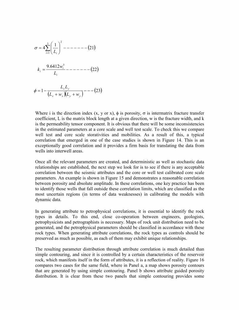
Log Analysis Naturally fractured carbonate reservoirs can also be evaluated using well logging techniques. Several methods are available to evaluate natural and induced fractures in the reservoir from well log data7. For example fracture and vuggy effects on porosity reflect on the measured total porosity from neutron, acoustic and density tools. The effect is also reflected in the cementation exponent, �m�, which represents the tortuosity of the reservoir rock. Usually the value of �m� is approximately equal to 2.0 for formations with interparticle (grains or crystals) porosity and the value for a plane fracture is technically equals 1.0. This is based on the relationship between formation resistivity factor, F, tortuosity, , porosity, � � , and the cementation exponent, m. These factors form the basis of our proposed methodology as shown in the sections that follows. Proposed Methodology. Typically, most naturally fractured carbonate systems are composed of other pore types including fractures, vugs, bimodal and intercrystalline. It is therefore important to review sedimentological and petrological study done on representative cores, sidewalls and cuttings. An example of such description for a carbonate reservoir rock system in the Gulf of Mexico is shown in Figure 2. This sedimentological data acts as a guide in the use of petrophysical cross plots to identify the pore types. Determination of pore types from series of Cross-plots To determine the pore types in the well, series of cross plots are typically performed to identify bimodal porosity, fracture porosity, vuggy porosity, Intercrystaline porosity, etc7. The following plots are needed for proper identification and differentiation

1. Sonic versus total porosity (Neutron) 2. MSFL Porosity versus total porosity (neutron) 3. Archie water saturation (n=2,m=2,a=1) versus ratio water saturation

The plots should look like figure 2.

Modeling Approach The relationship between cementation exponent and tortuosity is given by equation 1

below.

F RR

o

w

� ��

�--------------------------------(1)

F m�1�

---------------------------------------(2)

For plane fracture with tortuosity approximately equal to 1 it is easy to see that m is equal to 1. However, fractures are not plane and hence �m� can vary from one (1) up to 4 depending on (1) the intensity of fracturing and tortuosity (2) the relationship between fracture, vugs and matrix (3) Degree of mineralization (m>2 if fracture contains clay minerals). In applying this modeling concept, it is important to note that in addition to tortuosity, cementation exponent depends on (1) Specific surface area, (2) Grain shape

(3) Degree of Cementation (4) Clay content and location and (5) Level of pore interconnectivity. Variable �m� Model An important aspect in this modeling is the ability to determine variable �m�. The technique is described below. The first step is to determine the variation of reservoir rock quality with �m� or hence degree of fracture. For this permeability and porosity measurements as well as formation factors should be measured on a series of fractured full diameter cores representing the reservoir of interest. These measurements are made at simulated reservoir condition using the methods described earlier. As shown in Figure 3, an example of a carbonate reservoir in the Gulf of Mexico, core analysis data on fractured rock samples shows �m� varies from a low of 1.4 in the fractured zone to a high of 2.43 in the mineralized fracture or vuggy zones. This figure also shows that �m� is related to the reservoir quality and that fractures and fracture intensity control reservoir flow capacity. The �m� can also be estimated from log data. The following relationships and logic are used to compute variable �m� from logs and to account for the variable pore types (Fracture, Bi-modal, Vuggy and Intercrystaline):

)(

)(2

e

t

W

LOG

SWRTR

LOG

m R

�

��

�

�

��

�

�

�� -----------(3)

Where

� � 8/5

//

wmf

txoR RR

RRSW � -----------(4)

Pore types can be recognized as follows: m= 2� , Pore Type is Intercrysalline �

m>2, Pore Type is Vuggy m< 2, Pore Type is fractured or bi-modal m< 2, and �RXO > �T �� , Pore B-modal m< 2, and �RXO < �T �� , Pore Fracture Where, is some tolerance based on random errors. ��

Flow Properties Determination The core data is also used to develop equations for fractured reservoir flow properties modeling. Based on previous work1, for a naturally fractured or vuggy reservoir system, permeability is given as a function of total porosity, specific surface area and �m� as follows

2)1(

12F

12

gvS

t

tKm

s�

�

�

�

�

---------------------(5)

Therefore following the hydraulic (Flow) units (HU) concept8,9,10,11, we can define RQI for fractured systems as

12

K0314.0FRQI�

� mt�

--------------(6)

Hence Flow zone indicator for fractured system is defined as

sgv Fs1FRZI � --------------(7)

Hence

� �FRZIFRQI log)log( � + ----- (8) log( )� z

Note that FRZI is independent of the tortuosity rather than surface to volume ratio. Therefore, as in the HU concept for sandstone, a plot of FRQI versus �z on a log-log paper will delineate the flow units as shown in Figure 6. We use the following procedure to delineate hydraulically similar intervals: 1. Data required from core analysis include porosity, permeability and �m� from

whole core. 2. Discrete values of reservoir quality indicators (FRQI) are calculated from the

available data using EQ. 6. 3. Discrete values of �z are computed using the following equation.

�

�

���

1z

4. Then discrete values of flow zone indicators (FRZI) are calculated from the

available data using the following equation

z

FRQIFRZI�

�

5. Histogram of the discrete FRZI is constructed to determine the number of observable population based on the number of normal distributions.

6. Cluster analysis are then performed using the numbers of units predicted from step # 5 to separate the samples into clusters.

7. Log-Log plot of FRQI versus porosity group �z and semi-log plot of permeability versus porosity are made for the different cluster groups to delineate the HUs.

This information can then be used for log analysis in two ways, namely, System Response Analysis and Flow Zone Assignment based Calculated �m�

1. Systems Response Analysis This method is the best technique when large amounts of core analysis and log data are available. First a relationship is developed between FRQI and �m� from the representative core measurements. Such a relationship should look like as in Figure 4. The second and most important step in the systems response model is the development of training equations or model to determine FRZI from log signatures based on core-log integration. Three different methods are currently available to us for performing this task (1) probabilistic method (2) Neural Network method and (3) deterministic method (non-linear optimization). Probabilistic Method Qualitative predictions of FRZI for the wells without core data are achieved by using a probabilistic algorithm with a deterministic data. The deterministic data consist of Core derived FRZI, and a combination of corresponding log response. Note all wireline log data may correlate to FRZI hence the pertinent data are obtained through rank correlation as shown later. The Probabilistic method uses relationships implicit in the data to derive results without requiring any assumption or predetermined equations. Results are obtained by statistical inferences. Neural Network Method We currently use the Western Atlas computer package called HORIZONTM for our probabilistic modeling. This technique requires that the variables (FRZI) to be estimated be known in at least one or more intervals. QUERY, a Gaussian algorithm is used in a krigging process to estimate values of FRZI from a Histogram, LEARN.HST, created by the Learn module. The methodology can be explained simply by an analogy with the traditional Z-crossplot. In this crossplot, FRZI profile of the cored section(s) is placed on the Z-axis. All the other log responses form the other axes of the crossplot. Then, making statistical inferences to the database for each specific hydraulic unit creates FRZI profile of the uncored sections.

Artificial Neural Networks (ANN) are data processing mechanism which transform input data into desired output data using the internal architecture which is pattern after neuron-synapse models that describe the inner workings of the human brain. They use a multi-layer, back-propagation architecture that allows the artificial neural network to apply knowledge from training points to making prediction. ANN works very well at solving problems when it is difficult to propose exact mathematical models. Artificial neural networks learn the nature of the dependency between input and output variables through a carefully selected and representative set of training examples. We use neural networks to develop a flow zone indicator (FRZI) model to be used in solving the inverse problem: calculate FRZI in uncored intervals/wells. Deterministic Method This is the best method to compute the FRZI in the uncored intervals/wells without relying on any �black box�. FRZI computation from the cored wells/intervals is used in a

nonlinear optimization based on the Levenberg-Marquard non-linear optimization algorithm described by Ohen el at12. The minimization problem can be stated as follows:

� �xfRx

minn

�

------------------------ (9)

Where, f: �n � � is at least continuous. The Levenberg-Marquard routines for minimization used in this work based on the nonlinear least squares and it is part of IMSL Math Library13. The function f(x) is a combination of log response as determined from the rigorous rank correlation exercise described in next section. A typical combination of log signatures that may be used are a combination of spectral or total gamma ray (GR), neutron and density porosity differences (�N-D), neutron and sonic porosity differences (�N-S), bulk density (RHOB), Micro spherically Focussed logs (MSFL) etc. These log signatures are correlated to FRZI as follows and used in the Levenberg-Marquard non-linear optimization algorithm. FRZI = (GR,�N-D, �N-S, MSFL, RHOB) -------(10) 2. Flow Zone Assignment based on Calculated �m� This technique is used when available core data is not enough to perform the systems response analysis. From the limited core analysis data, average values of FRZI can be assigned to a range of �m� as shown later in the example. For the application of this methodology in log analysis, �m� is obtained from logs by Eqs. 3 and 4. Once FRZIave is obtained by either method, permeability can be calculated as follows.

2)1(

1221014

t

tFRZIKm

ave

�

�

�

�

�

----------------- (11)

Differentiating Between Matrix and Fracture Properties Fracture Porosity We used the following two concepts to characterize naturally fractured reservoirs: (1) the concept of partitioning coefficient, �, and (2) the concept of fracture intensity index, FII. Concept of Partitioning Coefficient, �. Partitioning coefficient, �, represents the allocation of total porosity, �t, between matrix porosity, �ma, and the larger pores (vugs, fissures, fractures, �f, etc.) and is given by:

�� �

� ��

�

�

t ma

t m( )1 a

. -------------------------(12)

Fracture Intensity Index, FII. FII represents the magnitude of formation porosity attributed to fractures as the ratio between secondary porosity (fractures) to the solid rock volume as:

FII t m

ma

�

�

�

� �

�1a . --------------------------(13)

Thus, FII is related to the partitioning coefficient, �, by: FII t� �� . -----------------------------(14)

� ��

�

��f

t

t

FII�

�

�

11

. --------------------(15)

We estimate partition coefficient as follows1 � ��

�

tm 1 . -------------------------(16)

Hence it can also be estimated as

FII t

m� � . .......................................................... (17)

Recall that formation resistivity factor is given by F t

m�

�

� = 1/FII ................................................. (18) Following these relationships, fracture and matrix porosities are given as follows:

�� �

�f

tm

tm

tm�

�

�

�1

1. .............................................. (19)

Matrix Porosity Matrix porosity can be computed as:

�� �

�ma

tm

t

tm�

�

�1. ................................................ (20)

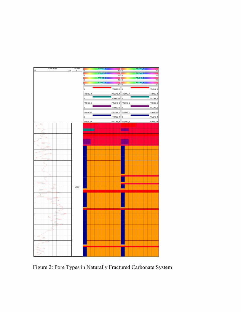
Example from the Gulf of Mexico In this example of a carbonate reservoir system from Gulf of Campeche, there was limited core data hence the flow zone assignment technique was used. From the limited core data the following four flow zones were identified as shown in Figure 5. Zone #1 �m� 1.65, FRZI� ave=89-------(17)

Zone #2 1.65<�m� 1.93, FRZI� ave =35.6----(18) Zone #3 1.93<�m� 2.3, FRZI� ave =14.24 ------(19) Zone #4 �m�>2.3, FRZIave =7.85 --------------(20) Using Eqs. 3 and 4, �m� values were estimated for all the wells and the range of �m� was used to assign FRZIave according to Eqs. 17-20. Zone 1 is considered a high conductivity fractured zone, zone 2 is dominated by fractures and vugs while zones 3 and 4 have mostly matrix permeability. This logic was used to determine the matrix and fracture permeabilities. Permeability associated with zones 1 and 2 are sorted as fractured permeability. As shown in Figure 6, the averaged total permeability per well for seventeen wells/zones is about two orders of magnitude less than the fractured permeability obtained using the method described in this work. Note that each point in Figure 6 represents a well/zone. Figure 7 is a fracture intensity map created from this information. Upscaling Based on the systematic procedure presented in the previous sections of this paper, a consistent data base for matrix and fracture petrophysical properties can be created together with the hydraulic units, RQI and FII. In this section we will discuss the utilization of this information in constructing and using engineering models. A typical reservoir study comprises the following essential steps; namely data collection; data processing; reservoir framework studies; data integration to generate reservoir model; upscaling to generate simulation model (see Figure 9); and dynamic calibration of the model (history matching); feasible technical scenario identification and the choice of a viable economic scenario for implementation. We will deal here only up to simulation model generation and its calibration with dynamic data. The first step involves data collection from different sources and scales and their processing at the observation points (wells) to obtain the required information. The discussion on the relative merits of each data collection method is beyond the scope of this paper. We will only focus some methodologies in relation to data scales. Following Table 1 summarizes the scale difference where it is clear that core plug is approximately 6.5E11 times smaller than well test domain used in the example. Table 1: Typical volume scales for different methods of data acquisition and their comparison with the well test scale

Method Typical Volume Scale (cft)

Relative Volume

Geologic Thin Section 3.5E-6 8E-15

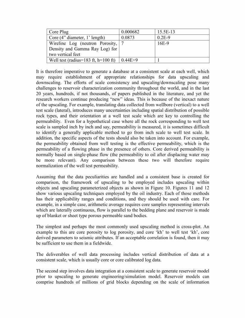
Core Plug 0.000682 15.5E-13 Core (4� diameter, 1� length) 0.0873 0.2E-9 Wireline Log (neutron Porosity, Density and Gamma Ray Log) for two vertical feet

7 16E-9

Well test (radius=183 ft, h=100 ft) 0.44E+9 1 It is therefore imperative to generate a database at a consistent scale at each well, which may require establishment of appropriate relationships for data upscaling and downscaling. The efforts of scale consistency and upscaling/downscaling pose many challenges to reservoir characterization community throughout the world, and in the last 20 years, hundreds, if not thousands, of papers published in the literature, and yet the research workers continue producing �new� ideas. This is because of the inexact nature of the upscaling. For example, translating data collected from wellbore (vertical) to a well test scale (lateral), introduces many uncertainties including spatial distribution of possible rock types, and their orientation at a well test scale which are key to controlling the permeability. Even for a hypothetical case where all the rock corresponding to well test scale is sampled inch by inch and say, permeability is measured, it is sometimes difficult to identify a generally applicable method to go from inch scale to well test scale. In addition, the specific aspects of the tests should also be taken into account. For example, the permeability obtained from well testing is the effective permeability, which is the permeability of a flowing phase in the presence of others. Core derived permeability is normally based on single-phase flow (the permeability to oil after displacing water may be more relevant). Any comparison between these two will therefore require normalization of the well test permeability. Assuming that the data peculiarities are handled and a consistent base is created for comparison, the framework of upscaling to be employed includes upscaling within objects and upscaling parameterized objects as shown in Figure 10. Figures 11 and 12 show various upscaling techniques employed by the oil industry. Each of those methods has their applicability ranges and conditions, and they should be used with care. For example, in a simple case, arithmetic average requires core samples representing intervals which are laterally continuous, flow is parallel to the bedding plane and reservoir is made up of blanket or sheet type porous permeable sand bodies. The simplest and perhaps the most commonly used upscaling method is cross-plot. An example to this are core porosity to log porosity, and core �kh� to well test �kh�, core derived parameters to seismic attributes. If an acceptable correlation is found, then it may be sufficient to use them in a fieldwide. The deliverables of well data processing includes vertical distribution of data at a consistent scale, which is usually core or core calibrated log data. The second step involves data integration at a consistent scale to generate reservoir model prior to upscaling to generate engineering/simulation model. Reservoir models can comprise hundreds of millions of grid blocks depending on the scale of information

chosen. In addition, this is the area where the inexactness of the upscaling and the level of error in data collection and processing manifest themselves much clearly. The cross-plots generated at the well bore and the data statistics generated from �vertical data (wells)� are assumed to be valid laterally. Deterministic method like interpretative contouring and the statistical techniques like geostatistics are used widely. The generated realizations are tested against some known geological rules and the accumulated knowledge base in the companies to enhance their degree of realism. Figure 13 shows various different geostatistical methods used to generate interwell data. The insert below shows a map of permeabilities of a North Sea Field using Kriging. Insert: Kriging results for a North Sea Field Over the last two decades Geostatistical methods were used widely and sometimes at the expense of the nature of the parameters distributed. For example, permeability is a tensor of the porous media, and it has directional components. It cannot simply be krigged to distribute it fieldwide. Tensor characteristics should be resolved in the first place. Next, permeability becomes a fact if there is a flow, so porous permeable rock units in areal sense to be identified, and kriging should be controlled by these units. These methods should therefore be applied under strict geoscience and engineering control. The deliverables of this stage will be scale consistent (say Core scale) parameter distributions which can be 3-D grids or property maps. The third step is the generation of the reservoir simulation/Engineering Model, which normally requires upscaling due to the computational restrictions. The methods presented above are used widely to come up with acceptable upscaling. The main challenge here is not to loose the important fine scale details (those, which will have profound impact on the reservoir dynamics) while upscaling. For example, in a given fractured reservoir, the principal stress direction of the reservoir can dominate the orientation of the fractures creating a fieldwide anisotropy. If this aspect is not preserved in the upscaling, the calibration and forecasting will not be consistent and realistic.

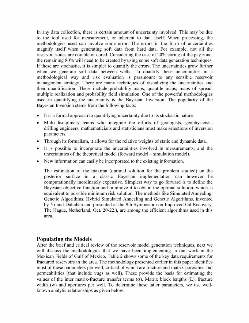
In any data collection, there is certain amount of uncertainty involved. This may be due to the tool used for measurement, or inherent to data itself. When processing, the methodologies used can involve some error. The errors in the form of uncertainties magnify itself when generating soft data from hard data. For example, not all the reservoir zones are corable or cored. Considering the case of 20% coring of the pay zone, the remaining 80% will need to be created by using some soft data generation techniques. If these are stochastic, it is simpler to quantify the errors. The uncertainties grow further when we generate soft data between wells. To quantify these uncertainties in a methodological way and risk evaluation is paramount to any sensible reservoir management strategy. There are many techniques of visualizing the uncertainties and their quantification. These include probability maps, quantile maps, maps of spread, multiple realization and probability field simulation. One of the powerful methodologies used in quantifying the uncertainty is the Bayesian Inversion. The popularity of the Bayesian Inversion stems from the following facts:

�� It is a formal approach to quantifying uncertainty due to its stochastic nature. �� Multi-disciplinary teams who integrate the efforts of geologists, geophysicists,

drilling engineers, mathematicians and statisticians must make selections of inversion parameters.

�� Through its formalism, it allows for the relative weights of static and dynamic data. �� It is possible to incorporate the uncertainties involved in measurements, and the

uncertainties of the theoretical model (forward model � simulation model). �� New information can easily be incorporated to the existing information.

The estimation of the maxima (optimal solution for the problem studied) on the posterior surface in a classic Bayesian implementation can however be computationally inordinately expensive. Simplest way to go forward is to define the Bayesian objective function and minimize it to obtain the optimal solution, which is equivalent to possible minimum risk solution. The methods like Simulated Annealing, Genetic Algorithms, Hybrid Simulated Annealing and Genetic Algorithms, invented by Yi and Daltaban and presented at the 9th Symposium on Improved Oil Recovery, The Hague, Netherland, Oct. 20-22.), are among the efficient algorithms used in this area.

Populating the Models After the brief and critical review of the reservoir model generation techniques, next we will discuss the methodologies that we have been implementing in our work in the Mexican Fields of Gulf of Mexico. Table 2 shows some of the key data requirements for fractured reservoirs in the area. The methodology presented earlier in this paper identifies most of these parameters per well, critical of which are fracture and matrix porosities and permeabilities (that include vugs as well). These provide the basis for estimating the values of the inter matrix-fracture transfer terms (�), Matrix block lengths (L), fracture width (w) and apertures per well. To determine these latter parameters, we use well-known analytic relationships as given below:

� �21143

1

2

����������

����

�� �

�i iL�

� �226412.9 3

��������

i

ii L

wk

� �� �� �231 ���

��

��

yyxx

yx

wLwLLL

�

Where i is the direction index (x, y or x), � is porosity, � is intermatrix fracture transfer coefficient, L is the matrix block length at a given direction, w is the fracture width, and k is the permeability tensor component. It is obvious that there will be some inconsistencies in the estimated parameters at a core scale and well test scale. To check this we compare well test and core scale storativities and mobilities. As a result of this, a typical correlation that emerged in one of the case studies is shown in Figure 14. This is an exceptionally good correlation and it provides a firm basis for translating the data from wells into interwell areas. Once all the relevant parameters are created, and deterministic as well as stochastic data relationships are established, the next step we look for is to see if there is any acceptable correlation between the seismic attributes and the core or well test calibrated core scale parameters. An example is shown in Figure 15 and demonstrates a reasonable correlation between porosity and absolute amplitude. In these correlations, one key practice has been to identify those wells that fall outside these correlation limits, which are classified as the most uncertain regions (in terms of data weaknesses) in calibrating the models with dynamic data. In generating attribute to petrophysical correlations, it is essential to identify the rock types in details. To this end, close co-operation between engineers, geologists, petrophysicists and petrographists is necessary. Maps of rock unit distribution need to be generated, and the petrophysical parameters should be classified in accordance with these rock types. When generating attribute correlations, the rock types as controls should be preserved as much as possible, as each of them may exhibit unique relationships. The resulting parameter distribution through attribute correlation is much detailed than simple contouring, and since it is controlled by a certain characteristics of the reservoir rock, which manifests itself in the form of attributes, it is a reflection of reality. Figure 16 compares two cases for the same field, where in Panel a, a map shows porosity contours that are generated by using simple contouring. Panel b shows attribute guided porosity distribution. It is clear from these two panels that simple contouring provides some

details around the wells, but away from wells, it smoothes the data. This type of parameterization creates enormous difficulties when calibrating the models using dynamic data especially when the recovery mechanisms modeled includes displacement. Attributes not only help the reservoir engineers but also the exploration team to a greater extent as well as they provide firm basis in structure definitions, identification of potential productive zones, and in avoiding blind drilling. In cases where oil base mud is used and it is not possible to split the total porosity into fracture and matrix porosity, and the permeability into matrix and fracture permeability, we implement a methodology based on �Edge� maps obtained from seismic attribute analysis. It is not as vigorous as the methodology discussed above, but provides database that is consistent with the field stress regimes and the rock deformation domains. The methodology used may be summarized as follows:

�� Create seismic attribute maps that demonstrate the existence and spatial

distribution of fractures and vugs. �� Contour those attributes that correspond to fractures and vugs only. �� Identify cut offs that differentiate the fractures and vugs �� Locate the vugs, and assign 100% porosity to those locations. �� Locate fractures and normalize the corresponding attributes �� Assume a minimum matrix block size in the presence of maximum

fracture density identified from seismic attributes. Maximum is when fracture density is zero.

�� Generate matrix block size distribution maps. �� Calculate fracture porosity and fracture permeabilities using correlations

based on the grid block sizes estimated from above �� Identify those locations where there are vugs, and enter 100% for

porosities and very high permeability values (in this case we used 1000 mD as cut off)

�� Use straight-line relative permeability relationships for the fracture system to characterize multi-phase flow.

�� Use the average parameters for a given layer and adjust the porosities and permeabilities accordingly

This way of generating interwell data is more reliable than any of those geostatistical techniques discussed before, as it dramatically minimizes the level of uncertainty of parameter estimation in terms of their quantities, and spatial distribution. The quality of these predictions can be further improved if 4 component (proper resolution of P and S waves) and 4-D seismic data available in late field life. In North Sea, the presence of constant sea bed monitoring using fixed source and geophones provides enormous amount of useful data for enhancing the confidence in generating interwell data as well as fluid contact determination. In fractured reservoir characterization, it is absolutely important not to use cut-offs for permeabilities and especially porosities as cut-off. This is because, for example, fracture

porosities can be as small as 0.0001 but the permeabilities can be as high as 1-10 Darcy for such porosities. By using cut-offs, it is possible that reservoir connectivity and hence the energy source is destroyed to a great extent. Instead, we recommend looking into pore connectivity as criteria, and this requires extensive petrographical work including the use of carefully selected thin sections. The deliverables of this stage of the work will be the maps of permeabilities, porosities, the matrix block sizes, and intermatrix fracture transfer terms. Relative permeability and capillary pressure is another important area especially for fractured reservoirs. This is because flow is not only in the matrix but in the fractures as well. In addition, the determination of multi phase flow between matrix and fracture requires specially calibrated relative permeabilities, which may be totally different than those for matrix and fractures. Normally fracture relative permeabilities are taken as straight line and no end points are assumed. This is an idealistic assumption, and ignores the fracture surface roughness, discontinuities, and possible capillary effects that may cause entrapment of the fluid in the reservoir fractures. Hence, as part of special core analysis study, it is important to elaborate the fracture characteristics even at a micro scale. This is usually done by using X-RAY Tomography techniques, and NMR. Relative permeability tests are then carried out to obtain relative flow characteristics of matrix, fracture, and matrix-fracture mass interchange. At times, it may also be necessary to identify the changes in the relative permeability shape and end points with pressure for particularly overpressured reservoirs. The presence of asphaltene is another problem area, and the formation damage due to its deposition not only manifests itself in terms of permeability decrease, but also changes in the wettability and thus the relative permeability characteristics. Identification of asphaltene deposition and generation of asphaltene deposition envelope (ADE), its reflection on the flow characteristics is one of the key aspects of the performance modeling efforts in the Gulf of Mexico. The determination of capillary pressure consistent with the field also plays major role as it helps to determine accurate fluid in place, and to model the displacement as well interfracture matrix mass transfer. It also plays significant role in gravity drainage process. In the Gulf of Mexico modeling efforts, we also use relative permeability and capillary pressure hysteresis, where the drainage curves are to model the initial fluid distribution, and the imbibition for the displacement modeling in general. Figure 17 shows one of the capillary pressure and relative permeability curves used in our studies. Last but not east is the distribution of the relative permeabilities laterally. We have been implementing facies or genetic flow unit controls in the relative permeability distribution and end point scaling. To this end, the methodology implemented may be summed up as follows: �� Identify and generate rock type distribution maps per selected flow (or engineering)

units. �� For each rock type of engineering units, compile relative permeabilities and generate

characteristic rock relative permeability and capillary pressure curves in normalized forms.

�� Using core and log data, generate end point saturations, end point relative permeabilities, maximum capillary pressures and threshold pressures per well, and where possible using attribute cross-plots distribute them areally for each rock type. If no attributes re available, we resort either contouring or stochastic techniques. By this way, we respect the general characteristics of the rock types, and generate unique saturation dependent parameterization for each rock type.

�� The normalized characteristic rock curves are then de-normalized at any point in space to obtain a saturation table.

The rock compressibility in fractured reservoirs is another challenge area. This is because the rock permeabilities can show dramatic changes with pressure. In addition to elastic deformation of the rock, plastic deformation can also result especially in the vicinity of the well bore. To this it is possible to add contractional rock failures in near well bore regions of the water injectors due to temperature changes. During flow simulation, changes in effective normal stress resolved across each fracture need to be estimated as a function of local reservoir pressure and fracture orientation. This modified normal stress need to be translated into a change in fracture aperture and fracture transmissibility. At this moment, there is no comprehensive and robust software available to handle hydraulic-mechanical- and thermal flow and the reservoir reaction to stress. They are at best approximations. In modeling efforts, knowing these limitations, we modify the transmisibilities explicitly. In the Gulf of Mexico, many reservoir characterization, dynamic calibration of engineering models, and performance predictions have been performed using the techniques discussed in this paper. One case is shown in Figure 19 where the solid circles show the measured static well pressures at different times. The challenge here has not only been to capture the reservoir pressure behavior, but also well static pressures using �stress reactive� rock properties. The general pressure trend of the model was following a consistent pattern displayed by the measured data, and at the shut in points, the match was excellent. This has not only been due to the high quality of data in the vicinity of the well bore but also due to the proper characterization of rock reaction to the pore pressure changes. Conclusions 1. A systematic methodology to petrophysical evaluation of fractured reservoirs is

presented. The benefits of this methodology may be summarized as follows: �� The Hydraulic units concept enables us to determine how the reservoir quality

changes with fracture intensity and distribution, which manifest in terms or tortuosity of formation resistivity factor.

�� A comparison of the petrophysical parameter obtained from this more rigorous

method with previous interpretation shows a remarkable improvement.

2. Techniques of upscaling/downscaling the petrophysical data and the data coming from �rock physics� are presented in view of generating detailed reservoir models.

Also presented are the consistent methods of generating engineering models from reservoir models with particular reference to fractured reservoirs. Some key issues addressed in the paper are:

�� A scale consistency is paramount in any data processing and integration �� A special emphasis is necessary on identification of data peculiarities and

characteristics in general. �� When using Geostatitical techniques in the parameterization of the models, the

nature of the parameters need to be taken into account. An arbitrary kriging of permeability, for example would result in invalid flow patterns.

�� In generating �soft data� from �hard data�, it s paramount to use rock types as controls as each facies can exhibit unique property distribution.

�� Some of the petrophysical properties like porosity, permeability, and relative permeability end points are affected by reservoir stress regimes. These warrant detailed geomechanical study not limited to elastic but plastic deformation as well. Although some softwares are available in the market, they are still very much restrictive. We believe that a new software approach needs to be adopted to properly handle the reaction of reservoir rocks against pore pressure changes.

Nomenclature F = formation resistivity factor = tortuosity �����porosity m = cementation exponent Ro = resistivity of a 100% water saturated rock Rw = formation water resistivity Rt = true formation resistivity �e = effective porosity Rmf = mud filtrate resistivity Rxo = resistivity of the mud-invaded zone �RXO = porosity of the mud-invaded zone �T = total porosity K = permeability Sgv = grain specific surface area Fs = pore throat shape factor FRQI = reservoir quality index for fractured rock system. FRZI = flow zone index for fractured rock system. � = inter matrix-fracture transfer term L = matrix block length w = fracture width

References 1. Application of Conventional Well Logs to Characterize Naturally Fractured

Reservoirs with their Hydraulic (Flow) Units; A Novel Approach. Tarek Ibrahim Elkewidy, GeoRes 4D (Grant Geophysical); and Djebbar Tiab,

SPE, University of Oklahoma, paper SPE 40038.

2. Nondestructive Measurements of Fracture Aperture in Crystalline Rock Cores Using X Ray Computed Tomography

Rober A. Johns, John S. Steude, Louis M. Castanier and Paul V. Roberts. 3. New Developments in the Analysis of Cores From Naturally Fractured Reservoirs J.L. Bergosh and G.D. Lord, Terra Tek Core Services, paper SPE 16805. 4. New Core Analysis Techniques for Naturally Fractured Reservoirs. J.L. Bergosh and T.R. Marks, and A.F. Mitkus, Terra Tel Core Services, paper

SPE 13653. 5. The Measurement of Matrix and Fracture Properties in Naturally Fractured Cores. Xiuxu Ning, Jin Fan, S.A. Holditch and W.J. Lee, Texas A&M U, paper SPE

25898. 6. New Analytical Techniques for Core Analysis for Fractured Reservoirs. F.M. Dawson and K.C. Pratt, Geological Survey of Canada � Calgary 3303-33

St. N.W. Calgary, Alberta. 7. Naturally Fractured Reservoirs. Aguilea. R., PennWell Publishing Company, Tulsa, 1995. 8. Enhanced Reservoir Description: Using Core and Log Data to Identify Hydraulic

(Flow) Units and Predict Permeability in Uncored Intervals/Wells. Amaefule, J. O., Altunbay, M., Tiab, D., Kersey, D. and Keelan, D., paper SPE

26436, 1993. 9. Modern Core Analysis, Vol. 1-Theory Tiab D., Core Laboratories, Houston, Texas, 1993. 10. A Hydraulic (Flow) Units Based Model for the Determination of Petrophysical

Properties from NMR Relaxation Measurements. Ohen, A. H., Ajufo, A., and Curby, F., paper SPE 30626 presented at the 1995

SPE Annual Technical Conference and Exhibition held in Dallas, Texas, 22-25 October 1995.

11. Effective Petrophysical Fracture Characterization Using the Flow Unit Concept-San Juan Reservoir, Orocual Field, Venezuela, J.G. Rincones, R. Delgado, H. Ohen, P. Enwere, A. Guerini, P. Márquez, SPE 63072.

12. Simulation of Formation damage in petroleum reservoirs Ohen, A. H., and F. Civan, Paper SPE 19420, Advance Technology Series, April

1993, 27-35. 13. Identification and Reduction on Uncertainties in Automatic History Matching and

Forecasting. Daltaban,T.S. and Yi, T., presented at the 9th Symposium on Improved Oil Recovery, The Hague, Netherland, Oct. 20-22.), 1997.

Table 2: Some of the essential data for fractured reservoirs.

Matrix Fracture CommonData

km kf�m �fcr crNTG NTG �

DZm

kro kro krokrw krw krwkrg krg krgPcw PcwPcg Pcg

Figure 1: Effect of Permeability on Pressure Transient Curves.

POROSITY 0 20

DEPTHFT

PTDSC-1 0 10

PTDSC-2 0 10

PTDSC-3 0 10

PTDSC-4 0 10

0 PTDSC-1

PTDSC-1 PTLOG_1

0 PTDSC-2

PTDSC-2 PTLOG_2

0 PTDSC-3

PTDSC-3 PTLOG_3

0 PTDSC-4

PTDSC-4 PTLOG_4

PTLOG_1 0 1

PTLOG_2 0 1

PTLOG_3 0 1

PTLOG_4 0 1

0 PTLOG_1

PTLOG_1 PTDSC-1

0 PTLOG_2

PTLOG_2 PTDSC-2

0 PTLOG_3

PTLOG_3 PTDSC-3

0 PTLOG_4

PTLOG_4 PTDSC-4

4000

0

0

0

0

Figure 2: Pore Types in Naturally Fractured Carbonate System

Figure 3: fractures and fracture intensity control reservoir flow capacity.

1.00

1.0

0

Intercrystaline

Vuggy / Fracture

1.0

0

Intercrystaline / Fracture

Vuggy

Bimodal

�Sonic

�t(neutron)

�RXO

�T (neutron)

0

1.0

1.00

1.0

0

Intercrystaline

Vuggy

Fracture / Bimodal

0 1.0

Intercrystaline

Vuggy

DO LS

AN SS

Swa

Swr

m

N

Figure 4:Variable "m" from core analysis

m = 1.8236RQI-0.0925

R2 = 0.8632

1

1.5

2

2.5

3

0 0.5 1 1.5 2 2.5 3 3.5

RQI, microns

m

Figure 5: Fracture Flow Units Zonation

0.1

1

10

100

0.01 0.1 1�z, fraction

FRQ

I, M

icro

ms 12

K0314.0FRQI�

� mt�

Figure 6: Relationship Between Total Permeability and Fractured Permeability (Kf from fractured zones 1 and 2)

10

100

1000

10000

100000

1 10 100 1000Total Perm (K), mD

Frac

ture

d Pe

rm (K

f), m

D

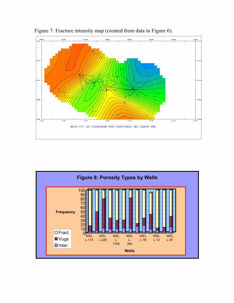
Figure 7: Fracture intensity map (created from data in Figure 6).

0102030405060708090

100

Frequency

WELL-11A

WELL-226

WELL-

176A

WELL-

39A

WELL-1B

WELL-12

WELL-35

Wells

Figure 8: Porosity Types by Wells

Fract.VugsInter.

Figure 9: Steps in a typical reservoir study.

Geologyand

Geophysics

Petro-physics

RCA+SCAL

Geo- Mechanics

WellTests

TracerTesting

DataDataAcquisitionAcquisition

Data Processing Data Processing and Integrationand IntegrationReservoir ModelReservoir Model

Up-scaling/Downscaling

SimulationSimulationModelModel

Up-scaling

Usually Millions of Grid Blocks

CORE SCALECORE SCALE

Validation/Validation/History MatchHistory Match

Technical Scenario

Economical Scenario

Figure 10: Framework of Upscaling Ak

BkCk

Dk

mk

fk

k

k

UPSCALINGWITHIN

OBJECTS

UPSCALINGPARAMETERIZEDPARAMETERIZED

OBJECTS

UPSCALINGRESERVOIRMODEL TOSIMULATIONMODEL

Figure 11. Upscaling Techniques

Ups

calin

gTe

chni

ques

Single Phase

Multi Phase

Analytic

Numerical

Analytical

Numerical

First Order

Higher Order

Figure 12. Upscaling Techniques (continued)

Simple ArithmeticArithmetic

Weighted Arithmetic

Thickness Weighted

Porosity WeightedFirst OrderUpscaling Porosity-Saturation

WeightedGeometric

Harmonic Arithmetic-Geometric

Hybrid Arithmetic-Harmonic

Arithmetic-Geometric-Harmonic

Som

ePe

rmut

atio

n

Figure 13: Geostatistical Techniques

Geo

stat

isti

csAuto-correlated

Permeability Field

Kriging

Standard Kriging

�Simple Kriging

�Ordinary Kriging

�Kriging withTrend

�Co-Kriging

�Indicator Kriging

�Markov-BayesModel

�Block Kriging

Conditional Kriging

Figure 14: Fracture porosity calibration to well test data

Fractured Porosity Calibration to Well Test Data

� fcal = a �fb

Fractured Porosity from Log

Frac

ture

d P

oros

ity fr

om

Equ

ival

ent W

ell T

est T

otal

P

oros

ity

Figure 15: Porosity versis absolute amplitude

Absolute Amplitude

Absolute Amplitude versus PorosityP

oros

ity

Figure 16: Panel a

Simple Porosity Contouring Figure 16: Panel b Attribute controlled Porosity distribution

Figure 17 Panel a

0 0.2 0.4 0.6 0.8 1

Imbibition Drainage Capillary PressurePc

Drainage

Imbibition

Sw

Figure 17 Panel b

0

0.1

0.2

0.3

0.4

0.5

0.6

0.7

0.8

0.9

1

0 0.2 0.4 0.6 0.8 1

Sw (Fraction)

kr (F

ract

ion)

krwkro

Figure 18: Using rock type control RELATIVE PERMEABILITY RELATIVE PERMEABILITY Rock-IndexingRock-Indexing

��������������������������������������

kro=(1-Se)n1

kro=(Se)n2

Swirr

Se

�

k

Sw

�

�

1-Sor

kro= k*ro(1-Se)n1

kro= k*rw(Se)n2

*rw

rwnrw*

ro

ronro

orwirrmaxw

wirrwk

k=k;

k

k=k;

S-S-SS-S

=Se

Normalization

Denormalization 1. Each grid blockwill have a set of relperms.

2. Increasing detail:Rel Perms arecontrolled by rocktype and attributes

Figure 19: Field �A history match

Field-A: History Match

Pres

sure

Time