Embed Size (px)
Citation preview
A Symplectic Acceleration Method for the Solution of the Algebraic Riccati Equation on a Parallel Computer
W. W. Lin
Institute of Applied Mathematics National Tsing-Hua University Hsin-Chu, Taiwan, R. 0. C.
and
s. s. You
Telecommunication Laboratories Ministry of Transportation Chung-Li, Taiwan, R. 0. C.
and Communications
Submitted by Volker Mehrmann
ABSTRACT
We give a cubic acceleration method for improving the current symplectic Jacobi-like algorithm for computing the Hamiltonian-Schur decomposition of a Hamil-
tonian matrix and finding the positive semidefinite solution of the Riccati equation. The acceleration method can speed up the rate of convergence at the end of the
symplectic Jacobi-like process when the norm of the current strictly J-lower triangle has become sufficiently small; it has high parallelism and takes O(n) computational
time when implemented on a mesh-connected n x n array processor system. A quantitative analysis of convergence and numerical comparisons of one Jacobi sweep
versus one correction step are presented.
1. INTRODUCTION
The problem of solving the algebraic Riccati equation
-XNX + XA + A*X + K = 0 (1.1)
LINEAR ALGEBRA AND ITS APPLICATIONS 188, 189: 437-463 (1993)
0 Elsevier Science Publishing Co., Inc., 1993
437
655 Avenue of the Americas, New York, NY 10010 0024-3795/93/$6.00
438 W. W. LIN AND S. S. YOU
(here A, K, N, and X are complex n X n matrices, N = N* > 0, and K = K* 2 0) arises for instance in linear-quadratic optimal control problems. It is assumed that (A, B) is stabilizable and (C, A) is detectable, where B and C are full-rank factorizations of N and K, respectively [9]. Under these assumptions, the equation (1.1) has a unique positive semidefinite solution which is equivalent to the problem of finding an n-dimensional invariant
subspace Y
[ 1 Z corresponding to the stable eigenvalues of the Hamiltonian
matrix
M= [“, _;*I. (1.2)
The solution of Equation (1.1) is then obtained by X = -ZY-‘. A matrix M
is called Hamiltonian if (JM)* = JM, where J is the 2n X 2n matrix
0 1 [ 1 -I 0
and I is the n X n identity matrix. It is well known that a Hamiltonian matrix is invariant under symplectic similarity transformations (a matrix S E C2”’ 2n is symplectic if S*jS = J). In 1981, Paige and Van Loan [ll] proved that, if the eigenvalues of M have nonzero real parts, then M has a Schur-Hamilto- nian decomposition, i.e., there exists a unitary symplectic matrix
Q= _;: F > [ 1 Ql> Q2 E CnXn,
1
such that
Q*MQ = [; $1 =R, (1.3)
where G* = G E CnXn, T E CnX” . 1s upper triangular, and the eigenvalues of T are in the left half plane. The matrix R in (1.3) is called a J-upper triangular matrix. Since
ALGEBRAIC RICCATI EQUATION 439
the desired nonnegative Hermitian solution of the Riccati equation (1.1) is given by X = Q2QI’ Ill].
Bunse-Gerstner and Mehrmann [2] and Ammar and Mehrmann [l] pro- posed the SR algorithm and SISHC algorithm, respectively, for solving the equation (1.1) on a sequential machine. Both methods preserve the Hamilto- nian structure. In the former, some intermediate transformation may fail to exist or may become very ill conditioned. But the latter uses only unitary symplectic transformations. The QR algorithm using unitary transformations, proposed earlier by Laub [9], unfortunately destroys the Hamiltonian struc- ture. However, the above three algorithms are not suitable for parallel processing.
In 1989, Byers [4] first proposed the symplectic Jacobi-like algorithm for the computation of the Hamiltonian-Schur decomposition of a Hamiltonian matrix. This algorithm requires O(n) computational time for a sweep when implemented on a mesh-connected n X n array processor system. It uses only unitary symplectic transformations and is close to the Jacobi-like method for a non-Hermitian matrix [12]. However, the convergence of Byers’s method [4] can be very slow if the Hamiltonian matrix is not near to normality; and very often the method does not converge at all for problems of dimension greater than 20. Recently, Bunse-Gerstner [3] developed a sym- plectic Jacobi-like algorithm for the computation of the Hamiltonian-Schur decomposition (1.3) based on the technique of Eberlein [7]. Each iterate in [3] needs only local information about the current matrix, thus admitting efficient parallel implementations on certain parallel architectures. The nu- merical experiments show that the convergence seems to be between linear and quadratic, which is much faster than the method in [4] when the matrices are far from normality.
The purpose of this paper is to describe an effective acceleration method (correction method) which can be used to speed up the rate of convergence at the end of the symplectic Jacobi-like algorithm in [3] or [4], when the norm of the strictly J-lower triangle of the current Hamiltonian matrix has become sufficiently small. The new method can be implemented on a mesh-con- nected rr X n array processor system in O(n) time.
In Section 2, we first briefly introduce the symplectic Jacobi-like (SJL) method (see [3, 41 for more details). Then, we propose a reordering tech- nique for eigenvalues and its parallel implementation. In Section 3, we derive some special matrix equations and then use these equations to develop a cubic symplectic acceleration method (SAM). This method is regarded as a corrector after some sweeps of the SJL method. A parallel processing for the SAM method and a Hermitian updating of an approximate solution of (1.1) are also given. In Section 4 we present a quantitative convergence analysis for the acceleration method. Theoretically, we prove that the SAM method
440 W. W. LIN AND S. S. YOU
convergences cubically. In Section 5, we compare the flop counts of the SAM method and the SJL method. The comparison shows that the SAM method needs fewer flops. Finally, we give some examples first computed by the SJL method and then corrected by the SAM method. Those results show that the accuracy of the solutions is almost twice more than that by the SJL method only.
We denote by I, (or I) the 12 X n unit matrix, by A* the complex conjugate transpose of an n x n matrix, and by B @ C the direct sum of matrices B and C.
2. SYMPLECTIC JACOBI-LIKE ALGORITHM
Byers [4] developed a symplectic Jacobi-like method for reducing the Hamiltonian matrix
to a J-upper triangular matrix (1.3) by Householder [ H(k, c, s)-rotation] and Jacobi [J(n, c, .s)-rotation] symplectic similarity transformations. These trans- formations, based on plane rotations, are used to annihilate the elements of K and the strictly lower triangular elements of A. We briefly describe these basic unitary symplectic rotations (see also [4]).
2.1. Householder Symplectic Rotation H(k, c, s>
Let
A, = ‘k,k ak,k+l
ak+l,k ak+l,k+l 1 be a 2 X 2 submatrix of A, and let [c, s]’ be a unit eigenvector of A,
associated with the eigenvalue h. Then the matrix
ALGEBRAIC RICCATI
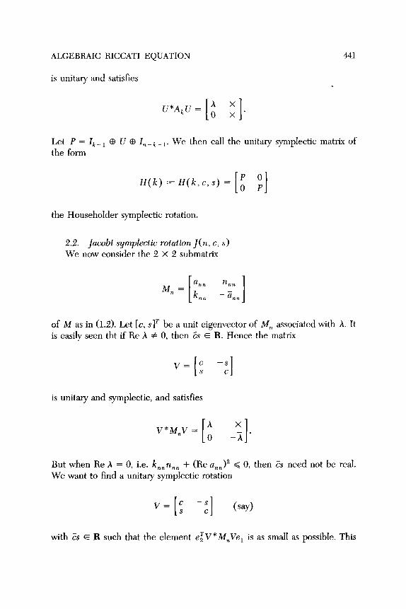
is unitary and satisfies
EQUATION 441
.
U*A,U = ; ; . [ 1
Let P = Zk_ 1 CB U CB I,, _k _ 1. We then call the unitary symplectic matrix of the form
H(k) := H(k,c,s) = P 0
[ I 0 P
the Householder symplectic rotation.
2.2. Jacobi symplectic rotation J(n, c, s> We now consider the 2 X 2 submatrix
of M as in (1.2). Let [c, slT be a unit eigenvector of M, associated with A. It is easily seen tht if Re A # 0, then Es E R. Hence the matrix
is unitary and symplectic, and satisfies
V*M,V =
But when Re h = 0, i.e. k,,n,, + (Re a,“)’ < 0, then Es need not be real. We want to find a unitary symplectic rotation
V=Z -: [ 1 (say)
with Es E R such that the element e:V *M,Ve, is as small as possible. This
442 W. W. LIN AND S. S. YOU
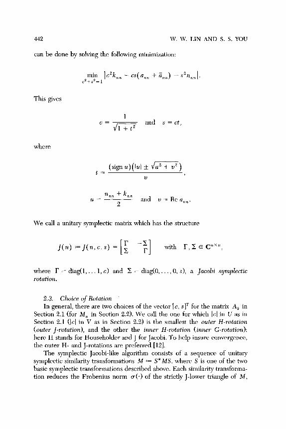
can be done by solving the following minimization:
min c*+s2= 1
c’k,” - cs(a,, + ii,,) - s2nnn I.
This gives
c=hG and s=ct,
where
t = (sip u)(lul * m) U
n nn + L U=
2 and u= Rea,,.
We call a unitary symplectic matrix which has the structure
J(n) :=J(n,c,s) = with r, 2 E cnXn,
where r = diag(1,. . . 1, c) and C = diag(0,. . . ,O, s>, a Jacobi symplectic
rotation.
2.3. Choice of Rotation
In general, there are two choices of the vector [c, s]r for the matrix A, in Section 2.1 (for M, in Section 2.2). We call the one for which [cl in U as in Section 2.1 (ICI in V as in Section 2.2) is the smallest the outer H-rotation
(outer J-rotation), and the other the inner H-rotation (inner G-rotation);
here H stands for Householder and J for Jacobi. To help insure convergence, the outer H- and J-rotations are preferred [12].
The symplectic Jacobi-like algorithm consists of a sequence of unitary symplectic similarity transformations M := S* MS, where S is one of the two basic symplectic transformations described above. Each similarity transforma- tion reduces the Frobenius norm o(e) of the strictly J-lower triangle of M,

ALGEBRAIC RICCATI EQUATION
where a(M) is defined by
443
l/2
I . Although the matrix M will converge to a J-upper triangular matrix by the
symplectic Jacobi-like algorithm [4], it is not guaranteed that the diagonal elements of M with negative real parts appear in T [as in (1.3)], which is necessary to get the nonnegative Hermitian solution of (1.1). Therefore, a reordering process is needed to arrange all diagonal elements of M with negative real parts appearing on the diagonal of T. A sequential reordering by unitary symplectic similarity transformations of this second pass was de- scribed in [2]. However, a parallel implementation of this reordering process is not trivial at all. The next subsection and Figure 1 describe this parallel implementation.
2.4. Reordering of the Eigenvalues and Parallel Implementation
We now consider the case when the SJL method converges. That is, for k = 1,2,. , . , the sequence M k + 1 = Qz M, Qk converges to a J-upper trian- gular matrix,
as in (1.3) with M, := M, where Qk is the product of the H- and J-rotations. Now, let Re t,, > 0, where t,, is the pth diagonal entry of T. We first
apply the Householder rotations H( p), . . . , H(n - 1) to move the element t pp to the (n, n> position of T, and then apply the Jacobi rotation J(n) to interchange t,, with -t [the (n, n) entry of the current -T*]. Here the H- and J-rotations are c i? osen so that the corresponding eigenvalues inter- changed. The following process formulates the interchange of the entry t,, of T with -tpp of -T*:
R^ :=J(n)*H(n - 1)” 0.. H( p)*RH( p) *.. H(n - l)](n). (2.1)
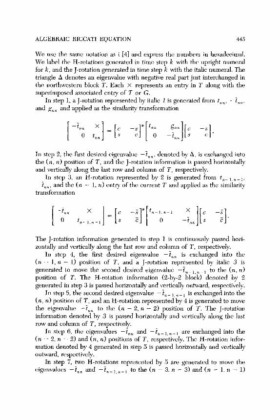
We exhibit in Figure 1 a useful strategy for devising a parallel implementa- tion of the interchange algorithm on the matrix T (n = 6) (the other matrices -T* and G are the same) for the worst case for reordering. That is, we consider the case that all diagonal elements of T having positive real parts.

444 W. W. LIN AND S. S. YOU
I
xxxxxx xxxxxx xxxxxx xxxxxx xxxxxx xXxXx1
5 xxxx22 x x x x.2 2 xxxxxx xxx443 22X443 22X33A
9 xxxx55 x77x55 x77xxx XXX176 55x776 55X666
13 AXXX80 XAAX88 XAAXXX XXXAA9 88XAA9 88X998
17 AXXXBB XAXXBB XXAXXX XXXDDC BBXDDC BBXCCA
21 AXXXDD XAXXDD XXAXXX XXXAXF EEXXAF EEXFFA
2 xxxxxx xxxxxx xxxxxx XXXXXl XXXXXl XXXIIA
6 xxxxxx xxx443 xxx443 X448X4 x44xx4 X33446
10 x77xxx 7AX776 7XX716 X77AX7 x77xx7 X6617A
14 AAAXXX AAXAA9 AXXAA9 XAAAXA XAAXXA X99AAA
18 AXXXXX XAXDDC XXADDC XDDAXD XDDXXD XCCDDA
22 AXXXXX XAXXXF XXAXXF XXXAXX XXXXAX XFFXXA
3 xxxxxx xXxXx1 xXxXx1 xxxxxx xxxx22 x11x22
7 xxx443 xxxxxx xx55xx 4X55XX 4xxx55 3xxx55
11 88X776 88XxX7 Xx88X7 7X88xX 7XXX88 677X88
15 AXXAA9 XAXXXA XXBBXA AXBBXX AXXXBB 9AAXBB
19 AXXDDC XAXXXX XXAXXX DXXAXX DXXXEE CXXXEE
23 AXXXXF XAXXXX XXAXXX XXXAXX XXXXAX FXXXXA
4 xXxXx1 xxxxxx xxxx22 xxxx22 Xx226X 1X22X3
8 xx55xx xx55xx 55AX55 55xx55 XX55AX Xx55X6
12 AX88XX XX88XX 88AX88 88xX88 xX886x Xx88X9
16 AXBBXX XABBXX BBAXBB BBXXBB XXBBAX XXBBXC
20 AXXXXX XAXXXX XXAXEE XXXAEE XXEEAX XXEEXF
24 AXXXXX XAXXXX XXAXXX XXXAXX XXXXAX XXXXXA
FIG. 1. The worst case for reordering.
ALGEBRAIC RICCATI EQUATION 445
We use the same notation as i [4] and express the numbers in hexadecimal. We label the H-rotations generated in time step k with the upright numeral for k, and the J-rotation generated in time step k with the italic numeral. The triangle A denotes an eigenvalue with negative real part just interchanged in the northwestern block T. Each X represents an entry in T along with the superimposed associated entry of T or G.
In step 1, a J-rotation represented by italic 1 is generated from t,,, -inn,
and g7l* and applied as the similarity transformation
In step 2, the first desired eigenvalue -t,,, denoted by A, is exchanged into the (n, n> position of T, and the J-rotation information is passed horizontally and vertically along the last row and column of T, respectively.
In step 3, an H-rotation represented by 2 is generated from t,_ r, n _ 1,
-t,,> and the (n - 1, n> entry of the current T and applied as the similarity transformation
The J-rotation information generated in step 1 is continuously passed hori- zontally and vertically along the last row and column of T, respectively.
In step 4, the first desired eigenvalue -t,, is exchanged into the (n - 1, n - 1) position of T, and a J-rotation represented by italic 3 is generated to move the second desired eigenvalue -i,_ 1, n_ i to the (n, n> position of T. The H-rotation information (2-by-2 block) denoted by 2 generated in step 3 is passed horizontally and vertically outward, respectively.
In step 5, the second desired eigenvalue - t,, _ i, n _ i is exchanged into the (n, n> position of T, and an H-rotation represented by 4 is generated to move the eigenvalue - tnn to the (n - 2, n - 2) position of T. The J-rotation information denoted by 3 is passed horizontally and vertically along the last row and column of T, respectively.
In step 6, the eigenvalues - 5,” and - 2, _ i, n _ i are exchanged into the (n - 2, n - 2) and (n, n) positions of T, respectively. The H-rotation infor- mation denoted by 4 generated in step 5 is passed horizontally and vertically outward, respectively.
In step 7, two H-rotations represented by 5 are generated to move the eigenvalues - t, n and - t, _ i. n _ i to the (n - 3, n - 3) and (n - 1, n - 1)
446 W. W. LIN AND S. S. YOU
positions of T, respectively. The H-rotation denoted by 4 and the J-rotation denoted by 3 are continuously passed outward.
In step 8, -t,, and -tn_l,n_l are exchanged into the (n - 3, n - 3) and (n - 1, n - 1) positions, respectively, and a J-rotation represented by italic 6 is generated to move the eigenvalue -t,_ 2 n_ 2 to the (n, n) position of T. The H-rotations denoted by 5 are passed horizontally and vertically outward, respectively.
Steps 9 to 12, 13 to 16, 17 to 20, and 21 to 24 are essentially similar to the procedure of steps 5 to 8, respectively. The H-rotations represented by 7, 8, A, B, D and E move the eigenvalues with negative real parts upward along the diagonal of T by exchanging the desired eigenvalues with the adjacent diagonal elements stepwise. The J-rotations represented by italic 9, C, and F are generated to move the desired eigenvalues with negative real parts to the (n, n> position of T, respectively.
It can be shown that the above parallel interchange algorithm requires at most 4n computational time for the general case. In practice, for large k, the matrix
M, =
approaches a J-upper triangular matrix. Hence, the diagonal elements of A, and -A: are close to the eigenvalues of M and pairwise well separated. Therefore, the interchange process can be applied if some diagonal elements of A, have positive real parts.
3. THE THE THE
SYMPLECTIC ACCELERATION METHOD AND NONNEGATIVE HERMITIAN SOLUTION FOR RICCATI EQUATION
In this section we develop an acceleration technique, the so-called symplectic acceleration method (SAM), for reducing the arithmetic cost for the case when the eigenvalues of the Hamiltonian M as in (1.2) are distinct. This method can speed up the rate of convergence at the end of the SJL method in Section 2 when the norm of the strictly J-lower triangle of M has become sufficiently small. In other words, M can be regarded as a perturba- tion of a J-upper triangular matrix. The main justification for this method is that the operations are very well suited to the mesh-connected system and the total computational cost is only O(n). Although our method, in its present form, is applicable only when the eigenvalues of M are distinct, this is in fact
ALGEBRAIC RICCATI EQUATION 447
the case for the matrices arising from a number of engineering problems of significant practical importance.
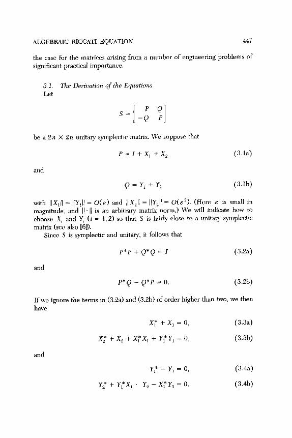
3.1. The Derivation of the Equations
Let
s=
be a 2n X 2n unitary symplectic matrix. We suppose that
P=z+x,+x, (3.la)
and
Q = Y, + Y, (3.lb)
with 11X,(] = l(Y,ll = O(E) and l]Xsll = /lYsll = 0(.s2>. (Here E is small in magnitude, and 1). 11 is an arbitrary matrix norm.) We will indicate how to choose Xi and Yi (i = 1,2) so that S is fairly close to a unitary symplectic matrix (see also [6]).
Since S is symplectic and unitary, it follows that
P*P + Q*Q = Z (3.2a)
and
P*Q - Q*P = 0. (3.2b)
If we ignore the terms in (3.2a) and (3.2b) of order higher than two, we then have
XT + x, = 0,
x,* + x2 + x,*x, + YCY, = 0,
(3.3a)
(3.3b)
and
r: - Y1 = 0,
Y,* + Ypxl - Y2 - XTY, = 0.
(3.4a)
(3.4b)
448 W. W. LIN AND S. S. YOU
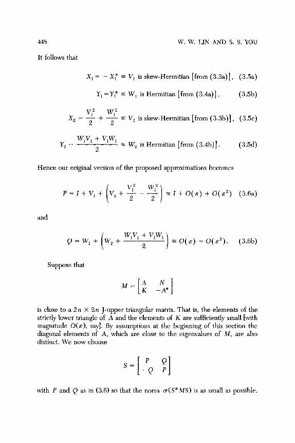
It follows that
x1= -x,x =v, is skew-Hermitian [from (3.3a)], (3.5a)
Y,=Y;k = w, is Hermitian [from (3.4a)] , (3.5b)
V: W: X, - T + --2- E V, is skew-Hermitian [from (3.3b)], (3.5~)
y2 - WlV, + VlWl
2 = W, is Hermitian [from (3.4b)] . (3.5d)
Hence our original version of the proposed approximations becomes
v,z wf V, + y - --2- = I + O(E) + 0( c’) (3.6a)
and
Suppose that
WlVl + VlWl 2
= 0( .s) + 0( E”). (3.6b)
is close to a 2n X 2n J-upper triangular matrix. That is, the elements of the strictly lower triangle of A and the elements of K are sufficiently small [with magnitude O(E), say]. By assumptions at the beginning of this section the diagonal elements of A, which are close to the eigenvalues of M, are also distinct. We now choose
s=
with P and Q as in (3.6) so that the norm (T(S*MS) is as small as possible.
ALGEBRAIC RICCATI EQUATION 449
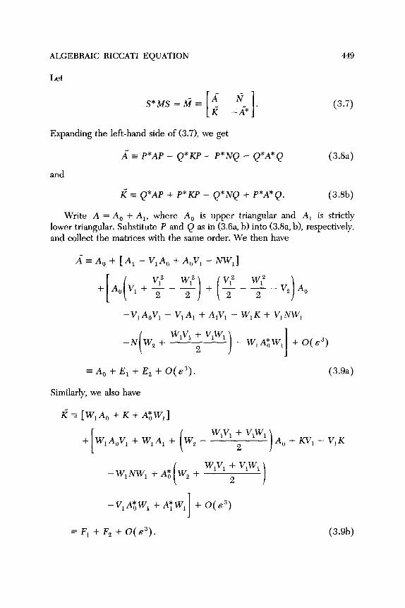
Let
(3.7)
Expanding the left-hand side of (3.71, we get
i = P*AP - Q*KP - P*NQ - Q*A*Q (3.8a)
and
K’= Q”AP + P*KP - Q*NQ + P*A*Q. (3.8b)
Write A = A,, + A,, where A, is upper triangular and A, is strictly lower triangular. Substitute P and Q as in (3.6a, b) into (3.8a, b), respectively, and collect the matrices with the same order. We then have
hA,+[A,-V,A,+A,V,-NW,]
v,z wf ----Vv,
2 2
-VI A,V, - V, A, + A,V, - W, K + V,NW,
w,v, + v,w, 2
- W,A;W, + 0(c3) I
(3.9a)
Similarly, we also have
K’= [W,A, + K + A;W,]
W, A,V, + W, A, + W,V, + V,W,
2 A,, + KV, - V, K
w,v, + v,w, 2
-V,A*,W, + ATW, + 0(c3) 1 = Fl + F, + O(c3). (3.9b)
450 W. W. LIN AND S. S. YOU
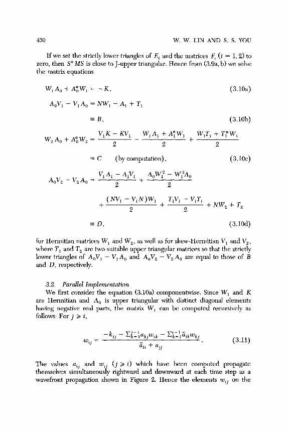
If we set the strictly lower triangles of Ei and the matrices F, (i = 1,2) to zero, then S*MS is close to J-upper triangular. Hence from (3.9a, b) we solve the matrix equations
W,A, + A;W, = -K, (3.10a)
A,V,-V,A,=NW,-A,+T,
E B, (3.10b)
W, A, + A*,W, = V,K - KV, W,A, + ATW,
+ W,T, + T: W,
2 - 2 2
EC (by computation), (3.1Oc)
A,V, - V, A,, = Vl Al - AlVl AaW; - W,2A,
+ 2 2
+ ( *1 - Vl N)Wl + TlVl - VlTl 2 2
+NW2+T,
= D, (3.10d)
for Hermitian matrices W, and W,, as well as for skew-Hermitian Vi and V, ,
where T, and T, are two suitable upper triangular matrices so that the strictly lower triangles of A,V, - V, A,, and A,V, - V, A, are equal to those of B
and D, respectively.
3.2. Parallel Implementation
We first consider the equation (3.1Oa) componentwise. Since W, and K are Hermitian and A, is upper triangular with distinct diagonal elements having negative real parts, the matrix W, can be computed recursively as follows: For j >, i,
wij = -k, - CiL:akjwik - c’-‘~ w k=l ik kj
Zii + ajj (3.11)
The values aij and wi. (j > i) which have been computed propagate themselves simultaneous y rightward and downward at each time step as a 1 wavefront propagation shown in Figure 2. Hence the elements wij on the
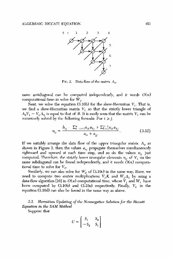
ALGEBRAIC RICCATI EQUATION 451
6
FIG. 2. Data flow of the matrix A,,.
same antidiagonal can be computed independently, and it needs O(n) computational time to solve for W,.
Next, we solve the equation (3.10b) for the skew-Hermitian V,. That is, we find a skew-Hermitian matrix V, so that the strictly lower triangle of A,V, - V, A, is equal to that of B. It is easily seen that the matrix V, can be recursively solved by the following formula: For i > j,
(3.12)
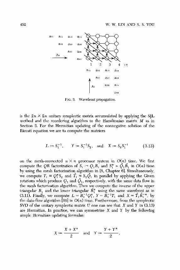
If we suitably arrange the data flow of the upper triangular matrix A, as shown in Figure 3, then the values uij propagate themselves simultaneously rightward and upward at each time step, and so do the values uij just computed. Therefore, the strictly lower triangular elements uij of V, on the same subdiagonal can be found independently, and it needs O(n) computa- tional time to solve for Vi.
Similarly, we can also solve for W, of (3.10~) in the same way. Here, we need to compute two matrix multiplications V, K and W,A, by using a data-flow algorithm [lo] in O(n) computational time, where V, and W, have been computed by (3.IOb) and (3.1Oa) respectively. Finally, V, in the equation (3.1Od) can also be found in the same way as above.
3.3. Hermitian Updating of the Nonnegative Solution for the Riccuti Equation in the SAM Method
Suppose that
U= SI ST.
[ I -s, s1
452 W. W. LIN AND S. S. YOU
1 2 3 4 :t
aI1 aI2 al3 ala
FIG. 3. Wavefront propagation.
is the 2n X 2n unitary symplectic matrix accumulated by applying the SJL method and the reordering algorithm to the Hamiltonian matrix M as in Section 2. For the Hermitian updating of the nonnegative solution of the Riccati equation we are to compute the matrices
L := s,l, Y := S,lS,, and X := S,S;’ (3.13)
on the mesh-connected n X n processor system in O(n) time. We first compute the QR factorization of S, := Q,R, and ST = Q,g, in O(n) time by using the mesh factorization_algorithm in [B, Chapter 61. Simultaneously, we compute T, = QT S, and T, ; S,Q, in parallel by applying the Given rotations which produce Qi and Qr, respectively, with the same data flow in the mesh factorization algorithm. Then we compute the inverse of the upper triangular R, and the lower triangular @ using the same wavefront as in (3.11). Finally, we compute L = R[‘QT, Y = R,‘T, and X = fig,*, by the data-flow algorithm [lo] in O(n) time. Furthermore, from the symplectic SVD of the unitary symplectic matrix U one can see that X and Y in (3.13) are Hermitian. In practice, we can symmetrize X and Y by the following simple Hermitian updating formulas:
x + x* Y + Y* x := ~ and Y := ~
2 2 *

ALGEBRAIC RICCATI EQUATION 453
Now, let
SC PQ [ 1 -0 P
be the 2n X 2n unitary symplectic matrix computed by the symplectic acceleration method, where P and Q are defined in (3.6). Since the set of the first n columns of the product of the matrices U and S,
is close to a basis of the invariant subspace corresponding to the stable spectrum of M, the matrix
i = (S,P + S,Q)(S,P - S,Q)-’
= (S,P + S,Q)P-‘(S, - S,QP-')-I
= (sz + S,QP-'&'(I - S2QP-1S;1)-1
= (S,S,’ + S,QP-%,‘)(I - S,QP-lS;‘)-l (3.15)
is then an approximation to the stable solution for the Riccati equation (1.1). We ignore the terms of order higher than two of the matrices P-’ and QP-l, and get
WlVl + VlWl 2 (1 - Vl)
= w, + w, + VlWl - WlVl 2 .
(3.16)
Next, substituting (3.16) into (3.15) and ignoring the terms of order higher
454 W. W. LIN AND S. S. YOU
than two of 2 again, we get
x’ = [S,S;' + S,(QP-')S;']
x [ Z + S,(QP-‘)S,’ + S,W,(S,S,)W,S;l]
= S,S;’ + S,(QP-‘)S,’ + S,S,lS,(QP-l)S,’
+s,s,‘s,w,( s,‘s,)w,s,’ + s,w,( s,‘s,)w,s,’
= S&r + S;*(QP-‘)S;’ + S;*W,(S;‘S,)W,S;’
because of the fact that
s, = s,* - s;*s2*s2 = s,* - S$,‘S, (3.17)
(since S, SC1 is Hermitian). From (3.13) we obtain the Hermitian updating formula of the approximate solution for the Riccati equation (1.1):
f=x-L* wl+wz+ ( VlWl - WlVl 2 1
L + L*w,YW,L. (3.18)
REMARK 3.1. If we are only interested in the nonnegative definite solution for (l.l), a Hamiltoniar$chur decomposition of M as in (1.3) is not necessary. That is, the matrix A in (3.9a) can be arbitrary. For convenience of computations we choose Vi 3 V, = 0 in (3.9b); then (3.9b) becomes
Ei = [W,A, + K + A;W,]
+ [Wi A, + Ws A0 - W,h’W, + A*,W, + AT W,]
+ WsA, + A;W, - (WsNW, + W,Nw,)
-P, + W,)(A, + 4)~
ALGEBRAIC RICCATI EQUATION 455
-W;(A; + AT) w, + w2
2 -W,hrW,
W$ + Kw,2 w$w: - +
2 4 1 = FI + Fz + Fs. (3.19b)
Ignoring the terms of order higher than two of K’ in (3.19b), we have the matrix equations
W,A, + A;W, = -K (3.20a)
and
W,A, + A;W, = -(W,A, + ATW,) + W,hW, (3.20~)
for the Hermitian matrices W, and W, , respectively. The Hermitian updating formula (3.18) can be reduced as follow:
x’= x - L*(w, + W,)L + L*w,yw,L. (3.21)
4. QUANTITATIVE ANALYSIS OF THE LOCAL CONVERGENCE
To use the symplectic acceleration method for finding the stable solution of Riccati equation, we have to solve the equations (3.2Oa) and (3.20~). Suppose the norms of A, and K as in (3.9) are O(E). (Here E is small in magnitude.) From (3.2Oa) and (3.20~) it is clearly seen that the norms of W, and W, are of order E and E ‘, respectively. Therefore, the norm of i in (3.19b) is of order c3, which is close to zero. Thus, the SAM method improves the result.
Now, we shall estimate the upper bounds for W, and W,. We define the separation of A,, and - AZ [13] by
Sep,( A,,, -A*,) = Inf{lD’WII~: IIWIIF = 1)
= Inf{llWA, + AEWllr : IIWIIF = I}, (4.1)
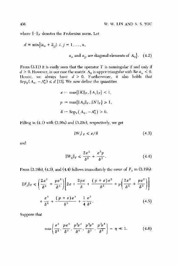
456 W. W. LIN AND S. S. YOU
where ]I * denotes the norm. Let
+ Zjj]:i,j l,..., n,
a,, and ujj are diagonal elements of A,,}. (4.2)
From (3.11) it is easily seen that the operator T is nonsingular if and only if d > 0. However, in our case the matrix A, is upper triangular with Re a,, < 0. Hence, we always have d > 0. Furthermore, it also holds that
Sep,( A,, -A: ) < d [13]. We now define the quantities
E := max{llKIIF, llA1ll~} < 1,
p := max{llAoll~, IINIIF} z 1;
6 := Sep,( A,,, -A*,) > 0.
Filling in (4.1) with (3.2Oa) and (3.20~1, respectively, we get
and
2E2 E2p IW,llF G - + - CT2 a3 *
(4.3)
(4.4
From (3.19b), (4.31, and (4.4) follows immediately the error of Fs in (3.19b):
E3 (p+&)E3 +LZ +-+
s2 S3 4 s4’ (4.5)
Suppose that
E3 ps3 p2E3 p2c4 -,-,- - 62 63 84 ’ ~5 ’ (4.6)
ALGEBRAIC RICCATI EQUATION 457
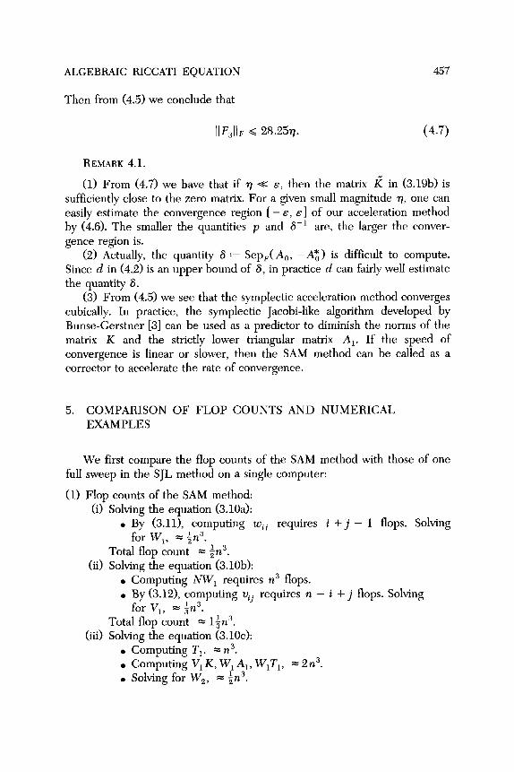
Then from (4.5) we conclude that
\]F,]]F Q 28.25~. (4.7)
REMARK 4.1.
(1) From (4.7) we have that if 77 << E, then the matrix i in (3.19b) is sufficiently close to the zero matrix. For a given small magnitude 7, one can easily estimate the convergence region [ - 6, E] of our acceleration method by (4.6). The smaller the quantities p and 6-l are, the larger the conver- gence region is.
(2) Actually, the quantity S := Sep,( A,, -AZ) is difficult to compute. Since d in (4.2) is an upper bound of 6, in practice d can fairly well estimate the quantity 8.
(3) From (4.5) we see that the symplectic acceleration method converges cubically. In practice, the symplectic Jacobi-like algorithm developed by Bunse-Gerstner [3] can be used as a predictor to diminish the norms of the matrix K and the strictly lower triangular matrix A,. If the speed of convergence is linear or slower, then the SAM method can be called as a corrector to accelerate the rate of convergence.
5. COMPARISON OF FLOP COUNTS AND NUMERICAL EXAMPLES
We first compare the flop counts of the SAM method with those of one full sweep in the SJL method on a single computer:
(1) Flop counts of the SAM method: (i) Solving the equation (3.1Oa):
. By (3.11), computing wij requires i + j - 1 flops. for W,, in”.
Total count = (ii) Solving equation (3.IOb):
Computing NW,
458 W. W. LIN AND S. S. YOU
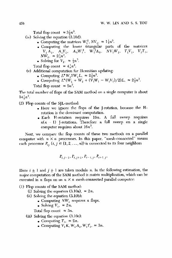
Total flop count = 3in3. (iv) Solving the equation (3.IOd):
. Computing the matrices W;“, NV,, = lin3. . Computing the lower triangular parts of the matrices
ViAi, A,V,, A,W,2, W:A,, NV,W,, T,V,, V,T,>
NW?., = 2+n3. . Solving for V,, = in”.
Total flop count = 4tn3. (v) Additional computation for Hermitian updating:
. Computing L*W,YW,L, = 2+n3.
. Computing L*(W, + W, + (V,W, - W,V,)/B)L, = 2+n3.
Total flop count = 5n3.
The total number of flops of the SAM method on a single computer is about 14$n3.
(2) Flop counts of the SJL-method: . Here we ignore the flops of the J-rotation, because the H-
rotation is the dominant computation. . Each H-rotation requires 16n. A full sweep requires
n(n - 1) J-rotations. Therefore a full sweep on a single
computer requires about 16n3.
Next, we compare the flop counts of these two methods on a parallel computer with n x n processors. In this paper, “mesh-connected’ means each processor Pij (i, j E {1,2, . . . , n}) is connected to its four neighbors
Pj,j_l, pi,j+l> pi-l,j, ‘i+l,j*
Here i f 1 and j + 1 are taken modulo n. In the following estimation, the major computation of the SAM method is matrix multiplication, which can be executed in n flops on an n X n mesh-connected parallel computer:
(1) Flop counts of the SAM method: (i) Solving the equation (3.1Oa), = 2n.
(ii) Solving the equation (3.IOb): . Computing NW, requires n flops. . Solving Vi, = 2n.
Total flop count = 3n.
(iii) Solving the equation (3.10~): . Computing T,, = 2n. . Computing Vi K, W, A,, WiTi, = 3n.
ALGEBRAIC RICCATI EQUATION 459
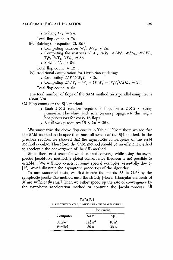
. Solving W, , = 2 72.
Total flop count = 7n. (iv) Solving the equation (3.1Od):
. Computing matrices Wf, NV,, = 2n.
. Computing the matrices V,A,, A,V,, AOWis, WtA,,, NV,W,, T,V,, VrT,, NW,, = 8n.
. Solving V,, = 2n.
Total flop count = 12n. (v) Additional computation for Hermitian updating:
. Computing L*W,YW,L, = 3n.
. Computing L*(W, + W, + (V,W, - W,V,)/2)L, = 3n.
Total flop count = 6n.
The total number of flops of the SAM method on a parallel computer is about 30n.
(2) Flop counts of the SJL method: . Each 2 X 2 rotation requires 8 flops on a 2 X 2 subarray
processor. Therefore, each rotation can propagate to the neigh- bor processors for every 16 flops.
. A full sweep requires 16 X 2n = 32n.
We summarize the above flop counts in Table 1. From them we see that the SAM method is cheaper than one full sweep of the SJL-method. In the previous section, we showed that the asymptotic convergence of the SAM method is cubic. Therefore, the SAM method should be an efficient method to accelerate the convergence of the SJL method.
Since there exist examples which cannot converge while using the asym- plectic Jacobi-like method, a global convergence theorem is not possible to establish. We will now construct some special examples, essentially due to [12], which illustrate the asymptotic properties of the algorithm.
In our numerical tests, we first iterate the matrix M in (1.2) by the
symplectic Jacobi-like method until the strictly J-lower triangular elements of
M are sufficiently small. Then we either speed up the rate of convergence by
the symplectic acceleration method or continue the Jacobi process. All
TABLE 1 FLOP COUNTS OF SJL METHOD AND SAM METHOD
Computer
Flop count
SAM SJL Single
Parallel 14: n3 16 n3 30 n 32 n

460 \ W. W. LIN AND S. S. YOU
numerical results are computed on an IBM PC in FORTRAN 77 with double precision. We use the following notation for Examples 4.1 and 4.2:
s := the number of Jacobi sweeps; u := the F-norm of the strictly J-lower triangle of the current M; y := the F-norm of the error matrix by applying the solution X to
the Riccati equation; i(IC) := after i Jacobi sweeps we perform the reordering (interchang-
ing) algorithm of eigenvalues of M; iSAM := after the step i - l(IC) we perform the symplectic accelera-
tion method.
EXAMPLE 5.1 (n = 5). Let
&f CYN a -D* _ Cyu* ” I
where D = diag( - 1, -2, - 3, -4, -5); N and U are, respectively, Hermi- tian and strictly upper triangular with entries randomly generated between + 1; and S is unitary symplectic. For different (Y ( LY = 0.01, 0.1, 1, lo), we have the numerical results given in Table 2.
EXAMPLE 5.2. Let
A=
4, 4, 0
A 22 A23
433 43, ’
0 A, -1
-1
where
r Ai,i+l = _y i )
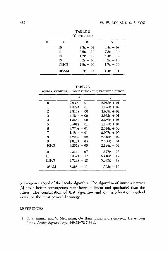
[ 1 and N = diag(1, 0, 1, . . . , 0, 11, K = diag(0, 10, 0, . . . , 10,O). The numerical result is given in Table 3.
From these two examples, we see that the symplectic acceleration method at least doubles the accuracy of the eigenvalues and significantly improves the

IACOBI ALGORITHM + SYMPLECTIC ACCELERATION METHOD
a S u Y
0.01 0 5.33 + 00 1 2 3
3(IC)
4 5
5(K)
4SAM
0.1 0 1 2 3 4
4(IC)
5 6 7
7(IC)
5SAM
1 0 1 2 3 4
4(X)
5 6 7
7(IC)
5SAM
10 0 1 5 7 8
&C)
2.0E + 00 1.8~ - 01 3.7E - 04 3.2~ - 04
8.2~ - 08 5.7E - 15 5.4E - 15
1.2E - 10
5.6~ + 00 2.0E + 00 2.0E - 01 1.6~ - 03 1.2E - 05 1.2E - 05
l.OE - 08 6.4~ - 12 5.8~ - 17 5.6~ - 17
2.3~ - 12
5.7E + 00 3.2~ + 00 5.7E - 01 3.9E - 02 2.4~ - 04 1.7E - 04
4.2~ - 06 3.03 - 08 2.9E - 11 2.5~ - 11
4.0E - 10
2.1E + 01 7.1E + 00 4.2~ - 01 5.03 - 02 5.6~ - 03 2.2E - 05 1.7E - 05
3.8~ + 00 1.5E + 01 2.3~ - 01 2.7~ - 03 3.4E - 05
4.5E - 07 1.1E - 14 %3E - 15
1.9E - 10
3.2~ + 00 1.8~ - 01 2.3~ - 01 2.0E - 02 1.4E - 06 5.4E - 05
1.8~ - 08 8.3~ - 12 4.4E - 17 6.2~ - 17
2.0E - 11
4.2~ + 00 5.3E + 01 6.1~ - 01 2.4~ - 01 1.2E - 03 8.8E - 04
1.2E - 06 2.3~ - 08 1.2E - 11 5.8~ - 11
1.73 - 09
1.4E + 01 1.3E + 01 1.8~ + 00 7.2~ - 02 1.6~ - 03 %3E - 06 1.6~ - 05
462
TABLE 2 (CONTINUED)
W. W. LIN AND S. S. YOU
CY s (T Y
10 2.3~ - 07 4.4~ - 08 11 6% - 10 7.5E - 10 12 1.2E - 12 4.4L? - 12 13 3.2~ - 16 8.2~ - 16 13(K) 2.8~ - 16 1.7E - 16
lOSAM 2.7~ - 14 1.4E - ll
TABLE 3 IACOBI ALGORITHM + SYMPLECTIC ACCELERATION METHOD
S o-
0 2.030~ + 01 1 1.322~ + 01 2 2.913E + 00 3 4.124~ + 00 4 1.865~ + 00 5 8.501~ - 01 6 4.770E - 01 7 1.184~ - 01 8 1.226~ - 02 9 1.816~ - 04 9CIC) 9.252E - 05
Y
2.018~ + 01 1.128~ + 02 3.937E + 02 3.652~ + 01 3.259E + 01 1.123~ + 01 2.024~ + 00 2.007~ + 00 2.545~ - 02 2.606~ - 04 2.188~ - 04
10 2.344~ - 07 1.677~ - 08
::(I0 5.3573 3.718~ - - 12 12 5.448~ 5.372~ - - 12 12
lOSAM 6.325~ - 11 1.3033 - 10
convergence speed of the Jacobi algorithm. The algorithm of Bunse-Gerstner
[2] has a better convergence rate (between linear and quadratic) than the
others. The combination of that algorithm and our acceleration method
would be the most powerful strategy.
REFERENCES
1 G. S. Ammar and V. Mehrmann, On Hamiltonian and symplectic Hessenberg forms, Linear Algebra A&. 149:55-72 (1991).

2 A. Bunse-Gerstner and V. Mehrmann, A symplectic QR like algorithm for the
solution of the real algebraic Riccati equation, IEEE Trans. Automat. Control
AC-31(12):1104-1113 (1986). 3 A. Bunse-Gerstner, On the Hamiltonian-Schur decomposition of a Hamiltonian
matrix, to appear. 4 R. Byers, A Hamiltonian-Jacobi algorithm, presented at SIAM Conference on
Control in the ’90s May 1989. 5 J. L. Casti, Dynamical Systems and their Applications: Linear Theory, Academic,
New York, 1977. 6 Roy 0. Davies and J. J. Modi, A direct method for computing eigenproblem
solutions on a parallel computer, Linear Algebra Appl. 77:61-74 (1986). 7 P. J. Eberlein, On th e c ur S h d ecomposition of a matrix for parallel computation,
IEEE Trans. Corn@. 36:167-174 (1987).
8 G. H. Golub and C. F. Van Loan, Matrix Computations, 2nd ed., Johns Hopkins U.P., Baltimore, 1989.
9 A. J. Laub, A Schur method for solving algebraic Riccati equations, 1EEE Trans. Automat. Control AC-24(13):913-925 (1979).
10 D. P. O’Leary and G. W. Stewart, Data-Flow Algorithms for Parallel Matrix
Computations, Computer Science Tech. Rep. 1366, Univ. of Maryland, 1984. 11 C. Paige and C. F. Van Loan, A Schur decomposition for Hamiltonian matrices,
Linear Algebra Appl. 41:11-32 (1981). 12 G. W. Stewart, A Jacobi-like algorithm for computing the Schur decomposition of
a non-Hermitian matrix, SIAM J. Statist. Cornput. 6(4):853-864 (1985). 13 G. W. Stewart, On the sensitivity of the eigenvalue problem Ax = ABx, S1AMJ.
Numer. Anal. 9(4):669-686 (1972).
ALGEBRAIC RICCATI EQUATION 463
Received 11 October 1990; final manuscript accepted 25 September 1992