A Switching Regression Model to Assess thePolicy Consequences of Direct Legislation ∗

Simon Hug†

CIS, IPZ, Universitat Zurich

December 6, 2007

Abstract

Most theoretical models predict that institutions allowing for directlegislation should lead, on average, to policies more closely reflecting thewishes of the voters. While some agreement exists at the theoretical levelabout the expected policy consequences of direct legislation, empirical ev-idence has been scant so far. In this paper I discuss the reasons for thisscantiness of empirical evidence, namely the intricacies of the adequateempirical model to test the theoretical proposition, and suggest possiblesolutions to this problem. Re-analyzing a dataset with which some au-thors have found no evidence in support of the theoretical claim, I showthat with a better adapted empirical model we find results in synch withour theoretical expectations. Thus, policies in states that allow for di-rect legislation reflect on average more closely the voters’ wishes. UsingMonte-Carlo simulations I also demonstrate the properties of the proposedestimator and suggest that it could be used in other contexts, like whenassessing the responsiveness of legislators.

∗ Earlier versions of this paper was presented at the Annual meeting of the Public ChoiceSociety, San Antonio, March 8-11, 2001 and at seminars at Texas A& M University, OhioState University, the University of St. Gallen and the University of Montreal. Thanks aredue to participants at these events and Chris Achen, Sven Feldmann, Mel Hinich, Tse-MinLin, John Matsusaka, Phil Paolino, and George Tsebelis for enlightening discussions on theintricacies of the statistical issues in this paper, and Ted Lascher for sharing his dataset. Partialfinancial support by the Swiss National Science Foundation (Grants No. 8210-046545, No. 5004-0487882/1, and No. 100012-108179) is gratefully acknowledged. I assume responsibility for allremaining flaws and errors.

† Center for Comparative and International Studies; Institut fur Politikwissenschaft; Uni-versitat Zurich; Hirschengraben 56; 8001 Zurich; Switzerland; phone +41 (0)44 634 50 90/1;fax: +41 (0)44 634 5098; fax: +41 (0)44 634 5098; email: simon.hug@access.unizh.ch

1

1 Introduction

Most research on direct legislation suggests that allowing voters to vote directly

on policies should affect policy outcomes (see Lupia and Matsusaka (2004) for an

incisive review of the literature). Scholars employing game-theoretic models to

assess these effects have mostly found that the policy outcomes should reflect more

closely the median voter’s preferences.1 Empirical studies have so far, however,

had difficulty demonstrating this effect convincingly. The reason for this is that

many empirical studies employ model specifications which either yield biased

estimates of the effect of direct legislation and/or do not allow for assessing

whether the policy is affected in the direction of the median voter’s preferences

(see Matsusaka’s (2001) discussion).

Consequently, I propose in this paper an empirical model, which derives di-

rectly from the theoretically implied predictions on the effect of direct legislation.

While the model is based on a simplifying assumption, its empirical evaluation

yields largely results in support of the theoretical implications on the effect of di-

rect legislation. In Monte Carlo simulations I also demonstrate that except under

very specific conditions, the proposed empirical model yields improved estimates

than a simple OLS regression with a dummy indicator for direct legislation states.

The paper proceeds as follows. In the next section I briefly review the litera-

ture on the policy effects of direct legislation. In section three I present first the

theoretically implied empirical model, before discussing specifications that have

been employed in the literature. I demonstrate that almost all of these specifi-

cations are based on erroneous assumptions which inevitably result in biases in

the estimated coefficients of relevance. In section four I present the results of

Monte Carlo simulations of the proposed empirical model for two setups. These

simulations demonstrate that the proposed empirical model provides better es-

timates and more information on the effect of direct legislation. In section five

I employ the proposed empirical model to assess the effect of direct legislation

using a dataset on the US states used by Lascher, Hagen and Rochlin (1996).

I demonstrate that with a more appropriate empirical model we find, contrary

to these authors, direct legislation effects for several policies, which are in ac-

cordance with predictions from theoretical models. Section six summarizes these

results and suggests that the proposed empirical model is also applicable in other

research areas, for instance when studying the responsiveness of legislators in

2

different institutional contexts.

2 The policy effects of direct legislation

There is a large consensus in the literature that institutions for direct legislation

affect policy outcomes.2 Only few authors, like for instance Cronin (1989, 232),

argue that policies do not differ between political entities allowing for direct

legislation and those that do not. From the early incisive writings of Key and

Crouch (1939), which were largely ignored by subsequent authors, it also seemed

clear that the policy effects of direct legislation may be of two different sorts.

First, the policy effects may be direct, in the sense that policies are adopted

by voters, which would have failed in the normal legislative process. Second,

institutions allowing for direct legislation may have indirect effects when the

legislature adopts policies which it would not have adopted without the presence

these institutions. Often such indirect effects emerge when interested groups

threaten legislatures with their own proposals, which they might try to realize

through direct legislation.3

These two types of effects appear especially clearly in recent theoretical work.

Steunenberg (1992), Gerber (1996 and 1999), Moser (1996), Besley and Coate

(2001), Matsusaka and McCarty (2001), Hug and Tsebelis (2002), and Hug (2004)

all show that the overall consequences of direct legislation comprise both direct

and indirect effects.4 From these theoretical models two other important elements

transpire. First, based on their theoretical implications it appears clearly that

sorting out direct from indirect effects empirically is difficult. This, because

these two effects interact and thus form the result of a strategic interplay among

various actors. Second, the theoretical models also demonstrate that the policy

effect of direct legislation, whether direct or indirect, is dependent on at least the

preferences of the legislature and the voters.5 The general thrust of the theoretical

results is that under most conditions, policies adopted under direct legislation

will be biased toward the preferences of the median voter.6 For example, if the

legislature would like to spend $ 1 million on a school building but the voters

prefer spending $ 2 million, then direct legislation will, on average, lead to higher

expenditures. Conversely, if the same legislature is on a spending spree and

wishes to construct a school-palace for $ 10 million, direct legislation will lead to

policies closer to the preferred spending level of the frugal voters. Consequently,

3

in one case direct legislation will lead to higher expenditures, while in the other

expenditures will be lower, due to direct citizen-lawmaking. This shows that the

effect of direct legislation is contingent on the preference configurations of the

most important actors, namely voters and the legislature.

In summary, the theoretical literature suggests that institutions for direct

legislation have both direct and indirect effects, but that these two types of effects

are difficult to separate empirically. In addition, the direction of these effects is

dependent on the voters’ preferences, in the sense that policies will reflect more

closely these preferences under direct legislation than in the absence of these

institutions.

3 Theory and empirical models

Strictly speaking the theoretical models mentioned above imply an empirical

model of the following type:7

|Yi −Xmi| = f(Xi) (1)

where Yi is a measure of a particular policy adopted in entity i, Xmiis the

median voter’s preferred policy in this area,8 and Xi contains an indicator variable

for the presence of direct legislation dli and possibly additional control variables.

If we had direct measures for both Y and Xm on the same scale, for instance

how much money is being spent for schools and how much money the median

voter wants to spend on schools, we could directly estimate equation 1. With the

possible exception of Gerber’s (1996) study on teenage abortions, we almost never

have data on the median voter’s preferences on the same scale as our measure

for the policy outcome.9 To see this problem it is useful to reformulate equation

1 in the following way:

ifYi −Xmi> 0

Yi = f(Xi) + Xmi

ifYi −Xmi≤ 0

Yi = −f(Xi) + Xmi(2)

4

In this setting it becomes clear that in the absence of a perfect measure of

what the median voter wants (e.g., what amount of money) we cannot estimate

equation 1 (or the system of equation 2 for that matter). Thus, if we have

to estimate Xmiwith proxies (like the often used conservative-liberal scale), we

cannot derive equation 2 directly from equation 1. We may presume that Xmi

is related to an array of variables Pi presumably linked to the preferences of the

median voter:

Xmi= g(Pi) (3)

Assuming (falsely) linear relationships for both equations 1 and 3 we get the

following system of equations:10

Xmi= Piβ + εi

|Yi −Xmi| = Xiγ + θi (4)

Our theoretical models would lead us to expect a negative value for the com-

ponent of γ measuring the effect of direct legislation. Assuming further that

εi ∼ N(0, σ2ε ) and θi ∼ N(0, σ2

θ) we may use equation 4 to derive the following

two equations:

if Yi −Xmi> 0

Yi = Piβ + Xiγ + εi + θi

if Yi −Xmi≤ 0

Yi = Piβ −Xiγ + εi − θi (5)

This system of equation can be rewritten in such a way that it becomes

a switching regression model with endogenous switching (Maddala 1983, 283),

where the superscript for Y indicates the regime:11

5

Y 1i = Piβ + Xiγ + εi + θi

Y 2i = Piβ −Xiγ + εi − θi

Ii = Yi − Piβ − εi

Yi = Y 1i if Ii > 0

Yi = Y 2i if Ii ≤ 0

(εi + θi, εi − θi,−εi) ∼ N(0, Σ) (6)

Here it becomes possible to compare the theoretically implied empirical model

as specified by equation 6 with other empirical models used in the literature.12

First, one predominantly used model attempts to assess the effect of direct legisla-

tion with a simple dummy indicator in a linear regression model (see for instance

Matsusaka 1995, 2000, 2004, Santoro and McGuire 1997, Kirchgassner, Feld,

Savioz, 1999, Santoro 1999). This traditionally used empirical model supposes

that the effect of Xi, i.e. the policy bias in non-direct legislation, is always either

positive or negative. If this is not the case, estimating a simple OLS model with a

dichotomous indicator for direct legislation states yields estimates biased toward

zero. Lascher, Hagen and Rochlin (1996) by adding in addition to the previous

model an interaction between the direct legislation indicator and a preference

measure probably attempted to allow for the conditional effect of preferences as

specified in equation 6. The system of equation, however, suggests that the effect

of preferences should not vary, but that the effect of the direct legislation dummy

is contingent on preferences. Finally, equation 6 also shows that Pommerehne’s

(1978a and 1978b) test based on the error variances between direct and non-direct

legislation states is not accurate, since the variances differ in a more complex way

between the two sets of states, except if we can assume that θ = 0.13

While the system of equation 6 provides a close approximation of the theoret-

ical models, a complication appears, however, in the estimation of the switching

regression model since the switching indicator Ii in equation 6 is not observed.

More spcifically, given that policy outcome (Y ) and preferences (P ) are mea-

sured in different scales, we do not observe whether a direct legislation state is

in regime 1 or regime 2 (see equation 6). As Lee and Trost (1978) and Mad-

dala (1983) show, the corresponding log-likelihood function (equation 8) is un-

bounded. In the original switching regression model with endogenous switching,

6

three distinct error terms appear in the first three equations of the system of

equation 6 (Maddala 1983, 283). Hence, the variance-covariance matrix in the

original switching regression models contains six different terms. As Lee and

Trost (1978) and Maddala (1983) demonstrate, not all six variance-covariance

terms can be estimated, given that they are not identified. Hence, restrictions

have to be imposed. The derivation of the model from theoretical implications

proposed here, however, leads only to two error terms, and thus three distinct

terms in the variance-covariance matrix:1

Σ =

σ2ε + σ2

θ + 2σε,θ σ2ε − σ2

θ −σ2ε − σε,θ

σ2ε − σ2

θ σ2ε + σ2

θ − 2σε,θ −σ2ε + σε,θ

−σ2ε − σε,θ −σ2

ε + σε,θ σ2ε

(7)

Hence the theoretical model from which the switching regression model here is

derived automatically leads to the restrictions on the variance-covariance matrix

necessary to estimate all the parameters of interest. The likelihood function under

the assumption of a normal bivariate distribution of the error terms ε and θ with

mean 0, variances σ2ε and σ2

θ and covariance σε,θ (possibly 0) is the following:14

llik = lnΠi[F (Yi −Xmi, σ2

εi)×

fN(Y − Piβ −Xiγ, σ2ε+θ|Yi −Xmi

> εi)

+(1− F (Yi −Xmi, σ2

εi))×

fN(Y − Piβ + Xiγ, σ2ε−θ|Yi −Xmi

≤ εi)] (8)

The estimation through maximization of equation 8 is simplified by the fact

that the variance-covariance matrix Σ (equation 7) only contains three distinct

elements, namely σ2ε , σ2

θ and σε,θ.15

4 Monte Carlo simulations

To assess the properties of the proposed switching regression model I carried

out a series of Monte Carlo simulations.2 To generate the datasets I used two

1This variance-covariance matrix follows directly from the error terms appearing in equation6 for Y 1, Y 2 and D.

2These simulations have two main objectives. First, given that the proposed empiricalmodel is based on a simplification, the simulations should show under what conditions this

7

setups. The first one was designed to correspond as closely as possible to the

empirical model, while the second one modeled the effect of direct legislation in a

more challenging way. In the first setup the data were generated in the following

way:16

P = 5 + 2 ∗X1 + ε

Y = 2 + 5 ∗ P + θ (9)

The independent variable X1 was generated as a random draw from a uniform

distribution over the unit-interval. To allow for correlation among the error terms

ε and θ were constructed in the following way:

ε = (1− j)× α1 + j × α2

θ =

{α2 + 2× α3 if dl = 0

α2 + 1× α3 if dl = 1(10)

where α1, α2, and α3 are drawn from three independent normal distributions

N(0, 1). If j = 0 ε and θ are uncorrelated. Letting j vary from 0 to 1, induces

increasing correlations in the error terms. In addition the proportion of states

with direct legislation (dl = 1) was varied from 0, to 0.25 and 0.5.17

This setup obviously quite closely reflects the empirical model proposed.

Hence, to carry out a more challenging test of the empirical model I also per-

formed Monte Carlo simulations with a second setup. In this latter setup, the

following relationships related the exogenous X1 to preferences and policy out-

come:

P = 5 + 2 ∗X1 + ε

Y =

P + 0 + θ if dl = 1

P + 1 + θ if dl = 0 and α > p

P − 1 + θ if dl = 0 and α ≤ p

(11)

α is drawn from a uniform distribution over the unit-interval and p was varied

from 0 to 0.25 and 0.5. In this setup policy deviates by 1 from the preferences

simplification still allows for correctly estimating the effect of direct legislation. Second, giventhat most studies assessing the effect of direct legislation rely on a small set of observations,the simulations should assess the small sample properties of the proposed estimator.

8

of the voters either in a positive or a negative direction in non direct-legislation

states. The value of p determines the proportion of states for which the effect

is in a negative direction. The frequently used model testing the effect of direct

legislation by simply estimating the effect for a dichotomous indicator implicitly

assumes that p = 0 (or p = 1). As p diverges from these extreme values, the

estimates from that traditional empirical model are biased toward zero. The

structure of the error terms was set up in the same way as in the first setup.18

In both setups 1000 samples for different sizes (i.e., 20, 50, 100, 200, . . . 1000)

were drawn. As Lee and Trost (1978), Maddala (1983) and Wilde (1998) note,

however, the performance of this estimator is quite sensitive to starting values. In

the Monte Carlo simulations this led to failures to reach convergence, especially

in runs with small sample sizes. Consequently for some combinations of sample

sizes, parameter values etc., only a small numbers of runs converged. Instead of

playing around with starting values,19 I report the results for these runs as well,

but by highlighting that they are based on smaller number of replications.

Figure 1 about here

The first results depicted in the eleven panels of figure 1 are based on the first

setup for the generation of the data. I report the mean estimate for the direct

legislation coefficient obtained from the switching regression (b mle sr) as well

as the one obtained from a simple linear regression (b ols) as a function of the

sample size.20 For each mean estimate I also report confidence intervals based on

the distribution of the estimated coefficients. Finally, each panel corresponds to

a different degree of correlation among the errors, going from values for j from 0

to 1 (see equation 10).

The results depicted in table 1 demonstrate essentially two things. First, the

OLS estimate is on average zero and thus suggests that direct legislation has no

impact on policy, while the estimate from the switching regression yields a mean

estimate very close to the true value, namely 1. Second, the confidence intervals

around these mean estimates shrink quite quickly from their large values for

small sample sizes when moving to larger samples. Only in the small samples

do the confidence intervals around the mean estimate of the switching regression

include the value 0. Both of these results are largely unaffected by increasing the

correlation between the error terms.21 Consequently, the switching regression

estimates give on average unbiased estimates of the main quantity of interest,

9

namely the coefficient for the direct legislation dummy. OLS regressions in this

particular setup of the Monte Carlo simulations are unable to detect the effect of

direct legislation, since the policy is not biased in the same direction in all states.

In the second setup, the switching regression model is more thoroughly tested

by varying the degree to which policy is biased in the same direction in non-direct

legislation states. In a first set of Monte Carlo simulations I set the proportion

of non-direct legislation states to 0.5, and in half of them policy is biased in a

negative direction, and in half in a positive one. The size of this effect is equal

to 1 again, however, given the way in which the data is generated, the coefficient

from the switching regression depends on the variances of the other components.

Figure 2 about here

For this reason I depict in figure 2 apart the confidence intervals for the

OLS and switching regression result only a line at 0, illustrating whether the

estimates on average show a significant effect for direct legislation.22 As for the

previous Monte Carlo simulations, the mean of the estimated OLS coefficients is

approximately 0, independent of the size of the sample or the correlation in the

error terms. In addition, the confidence intervals are again rather wide, implying

that we would systematically reject the hypothesis that direct legislation has an

effect on policy. The estimates from the switching regression model, on the other

hand, are systematically negative and for almost all sample sizes the confidence

intervals fail to include 0. Only for small sample sizes, i.e. 20, 50, 100 and 200,

is this not the case.23

Again this setup of the Monte Carlo simulations indirectly played in favor

of the switching regression model. Clearly if among the non-direct legislation

states the policy bias goes more frequently in the same direction, the switching

regression model will have a harder time detecting this effect. For this purpose

I designed two further Monte Carlo simulations. In the first a quarter of the

non-direct legislation states have a positive policy bias, while in the second this

proportion drops to zero.24

Figure 3 reports the result for the simulations where a quarter of the non-direct

legislation states have a positive policy bias.25 For small samples, neither the OLS

nor the switching regression estimates are accurate. The confidence intervals for

both estimators include the value of 0. With sample sizes of 300 or more, largely

independent of the correlation between the error terms, both estimators clearly

10

indicate an effect for direct legislation. Interestingly, the sample sizes starting

with which confidence intervals fail to include the value of 0 are largely the

same, though with a small advantage for the OLS estimator. The advantage of

the switching regression estimator, however, is that it gives clearly support to

the theoretically derived hypothesis, while the OLS estimator fails to yield this

information.

Finally, when the bias to policy is in the same direction in all non-direct

legislation states the results of the Monte Carlo simulations look as depicted in

figure 4. Not surprisingly in this case the tables are turned for the OLS and the

switching regression models. Since the policy bias goes in the same direction in

all non-direct legislation states, the OLS model with a simple dummy variable is

able to pick up this effect very well. Hence, the estimated coefficient is for all

sample sizes and correlations of the error terms approximately equal to 1. The

confidence intervals with increasing sample sizes diminish quickly and exclude

0 for most parameter combinations. The switching regression model, however,

yields mean estimates close to zero and also decreasing confidence intervals. The

reason for this is obviously that in the data there is no hint whatsoever that biases

may go in opposite directions. In the absence of such information, the switching

regression model is unable to detect this difference.

Figure 3 about here

Figure 4 about here

The Monte Carlo simulations of the switching regression model compared to

the simple OLS model clearly illustrated the strengths of the former. Provided

that the policy biases in non-direct legislation states are not systematically in the

same direction, the switching regression model gives us accurate estimates of the

policy bias that direct legislation allows to correct for. Only when the policy bias

in the non-direct legislation states is always or almost always in the same direction

does the OLS model with a simple dichotomous indicator give us a better answer.

While in such situations the OLS model is preferable, the estimates provided do

not allow us to draw any conclusions on whether the correction of the policy

bias due to direct legislation goes in the direction of the median voter or not.

Only information external to the model, like for instance the information that

Matsusaka (2000, 2004) has collected on contents of direct legislation proposals

and other information allow us to gain some insights in the direction of the policy

11

bias.

5 Policy consequences of direct legislation

While the Monte Carlo simulations already showed that the switching regression

model yields more information on the effect of direct legislation and also pro-

vides better estimates except under very specific conditions, concrete examples

may better illustrate the advantages of this estimator. To do so I use the data

employed by Lascher, Hagen and Rochlin (1996) (see table 1 for the policies em-

ployed26) to assess the effect of direct legislation in the US states. The basic

specification (see table 2) uses as independent variables the percentage of high

school graduates, the state per capita income, the percent of urban residents

and the ideology scale proposed by Erikson, Wright and McIver (1993). Lascher,

Hagen and Rochlin (1996) in addition use a dichotomous indicator for direct leg-

islation and an interaction term between this variable and the ideology scale. As

Matsusaka (2001) demonstrates, these authors erroneously interpret the coeffi-

cient for this interaction term as evidence for the effect of direct legislation and

essentially find no effect.

Table 1 about here

As in Lascher, Hagen and Rochlin (1996) these analyses only cover 47 states,

since according to Erikson, Wright and McIver (1993) the ideology measure for

Nevada, Hawaii and Alaska is unreliable, and these states are thus omitted.27

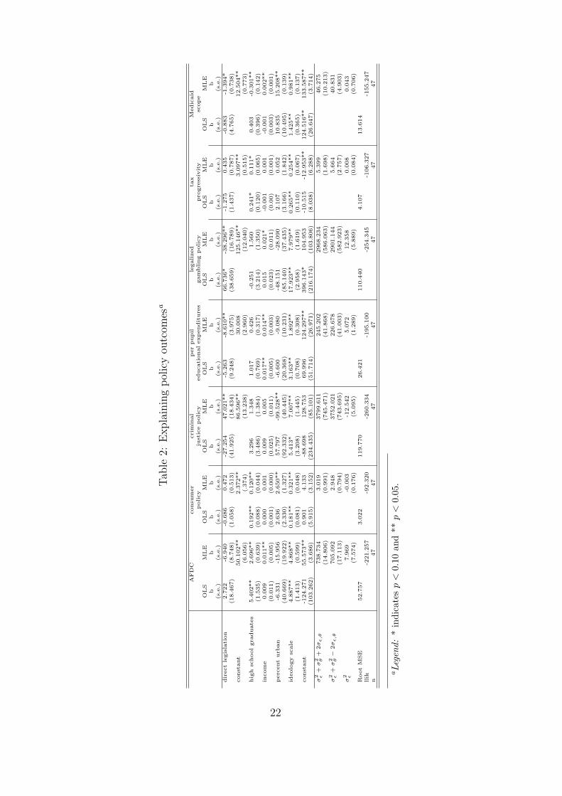
I report in table 2 for each of the seven selected policies first the result of a

simple linear regression with a dichotomous indicator for direct legislation states28

(columns OLS in table 2).29 The estimates for this variable vary from positive

to negative values and only for the policy of legalizing gambling is the estimated

coefficient statistically significant. Consequently, based on this empirical model

we would conclude that direct legislation only affects this particular policy in a

statistically significant way.

If we estimate the switching regression model (column MLE in table 2),30 we

find for four out of the seven policies, namely AFDC, educational expenditures,

gambling and Medicaid, negative coefficients for the direct legislation variable,

as expected by the theoretical model. Three out of these four negative estimated

coefficients are also statistically significant and thus provide clear support for

the hypothesis that direct legislation biases policy toward the preferences of the

12

voters. The three policies for which we find positive estimated coefficients are

the consumer and the criminal justice policy, as well as tax progressivity. Among

these three estimated coefficients, only the one for criminal justice policy reaches

statistical significance. This result suggests that in direct legislation states policy

outcomes differ more strongly from the voters’ wishes than in non-direct legisla-

tion states. Obviously this contradictory result is counterintuitive. Interestingly

enough, however, it is exactly for this policy and the tax policy where the prefer-

ence measures are most loosely related to policy outcomes.31 Hence, the negative

results are more likely to be related to the rather poor proxies for the voters’

preferences than to inherent problems with the proposed empirical model.

Nevertheless, the results reported in table 2 demonstrate that the proposed

switching regression model yields improved estimates for the effect of direct leg-

islation. Contrary to the results presented by Lascher, Hagen and Rochlin (1996)

we find for four of their policies effects for direct legislation as predicted by the

theoretical models. A frequently used model, namely the one estimating a coef-

ficient for a dichotomous direct legislation indicator, on the other hand, would

suggest policy effects only for one of these policies. Hence, the switching regres-

sion model is a clear improvement over existing models to test for the effect of

direct legislation. As the Monte Carlo simulations suggest, however, it should be

used in conjunction with the traditional models.

Table 2 about here

6 Discussion and conclusion

In the current discussion of the merits and drawbacks of direct legislation both in

the American states and around the world misguided generalizations often lead

to erroneous statements about the effect of direct legislation. Systematic studies

of the effect of direct legislation on policy outcomes (e.g., Matsusaka 1995, 2000

and 2004, Gerber 1996 and 1999, Gerber and Hug 1999, Kirchgassner, Feld and

Savioz 1999, Besley and Case 2003, Feld and Matsusaka 2003) come to more

nuanced conclusions than journalistic assessments (e.g., Schrag 1998 and Broder

2000) or analyses relying on case studies (e.g. Smith 1998).

But even among the more systematic studies it has often proved elusive to

find demonstrable effects of direct legislation on policy outcomes of the type we

would expect from theory. In this paper I argued that the reason for this elusive

13

quest is largely attributable to questionable empirical models. Based on the ba-

sic implication of most theoretical models, I derived an empirical model which

improves on the models currently used by researchers trying to show that direct

legislation has policy consequences. More precisely, this model directly acknowl-

edges the fact that the effect of direct legislation is contingent on the preferences

of at least the voters. Taking this into consideration in the empirical model I

employed in this paper, I was able to show that results obtained by Lascher, Ha-

gen and Rochlin (1996) are problematic and do not allow for the rejection of the

theoretically derived hypothesis. More precisely, using their dataset and using

both a simple empirical model testing for systematic policy biases in non-direct

legislation states and the one proposed here, I demonstrated that the improved

empirical model yields results largely in synch with theory and outperforms the

simple model.

This empirical investigation, however, is hardly sufficient to demonstrate the

merits of the empirical model proposed here. In Monte Carlo simulations I

also demonstrated that under most conditions, the proposed switching regres-

sion model provides more accurate estimates than a simple OLS regression. Only

under very specific conditions is the latter empirical model preferable. This sug-

gests that both models should be used simultaneously in order to assess the effect

of direct legislation. If a simple model with only a dummy indicator for the pres-

ence institutions for direct legislation yields a statistically significant coefficient,

we can reject the null-hypothesis that direct legislation fails to affect policy out-

comes. The size of the effect may, however, be biased toward zero and, in the

absence of additional information, we cannot be sure that the bias is toward the

median voter’s preferences.3 If the effect of direct legislation is not significant,

this may be due to the bias related to the empirical model or to a real absence of

an effect. In both cases, however, estimating the proposed switching regression

model would yield additional information. In the first case it might yield infor-

mation on whether policy is biased toward the voters’ preferences, while in the

second it might show whether the null-result is due to the misspecified model or

the real absence of an effect of direct legislation.

3More specifically, when only estimating a model with a dummy indicator for direct legisla-tion, extraneous information like in Matsusaka’s (2000, 2004) study comparing the fiscal effectsof direct legislation in two time periods has to be relied on to make arguments for the directionof these effects with regard to citizen preferences.

14

The use of the proposed empirical model is, however, not limited to assessing

the effect of direct legislation. In very diverse research areas similar questions

are raised and could be assessed with the same empirical model. Two areas

may be most prominent for this. First, and most closely related to the topic

of the present paper, the question whether in majoritarian political systems the

preferences of the median voter are more closely reflected in government (see for a

discussion Powell 2000) should lead to exactly the same empirical model. Second,

the literature on the responsiveness and representativeness of legislators is quite

clearly also dealing with the same effects. If we wish to assess the legislators’

responsiveness on particular policies the model proposed here may yield improved

insights32 Hence, future research first of all on the effects of direct legislation, but

also in other research areas should assess the applicability of the empirical model

proposed here.

15

7 Appendix

Table 3 reports the descriptive statistics of the variables employed in this paper

as well as their source. Table 4 reports the predicted probabilities for being in

regime 1 in the switching regression models (see equation 6).33

Table 3 about here

Table 4 about here

16

References

Achen, Christopher H. 1977. Measuring Representation: Perils of the Correlation

Coefficient. American Journal of Political Science. 21(4) 805-815.

Bartels, Larry M. 1991. Constituency Opinion and Congressional Policy Making:

The Reagan Defense Buildup. American Political Science Review . 85(2 June)

457-474.

Besley, Timothy and Anne Case 2003. Political Institutions and Policy Choices:

Evidence from the United States. Journal of Economic Literature 41(1) 7-74.

Besley, Timothy; Coate, Stephen 2001. Issue Unbundling via Citizens’ Initia-

tives . San Antonio: Paper prepared for presentation at the Annual Meeting

of the Public Choice Society, March 9-12.

Bowler, Shaun; Donovan, Todd. 2004. Measuring The Effects of Direct Democ-

racy on State Policy and Politics. State Politics and Policy Quarterly . 4 (3)

345-363.

Broder, David S. 2000. Democracy Derailed. Initiative Campaigns and the Power

of Money . New York: James H. Silberman Book/Harcourt.

Camobreco, John F. 1998. Preferences, Fiscal Policies, and the Initiative Process.

Journal of Politics . 60(AUG 3) 819-829.

Cronin, Thomas E. 1989. Direct Democracy. The Politics of Initiative, Referen-

dum and Recall . Cambridge: Harvard University Press.

Erikson, Robert S.; Wright, Gerald C.; McIver, John P. 1993. Statehouse Democ-

racy: Public Opinion and Policy in the American States . New York: Cam-

bridge University Press.

Feld, Lars P.; Matsusaka, John G. 2003. Budget Referendums and Government

Spending: Evidence from Swiss Cantons. Journal of Public Economics 87

2703-2724.

Gerber, Elisabeth R. 1996. Legislative Response to the Threat of Popular Initia-

tives. American Journal of Political Science. 40(1) 99-128.

Gerber, Elisabeth R. 1999. The Populist Paradox: Interest Group Influence and

the Promise of Direct Legislation. Princeton: Princeton University Press.

Gerber, Elisabeth R.; Hug, Simon 1999. Minority Rights and Direct Legislation.

Theory, Methods, and Evidence. La Jolla: Department of Political Science,

University of California, San Diego.

17

Gerber, Elisabeth R.; Hug, Simon 2001. Legislative Responses to Direct Legisla-

tion. in Mendelsohn, Matthew; Parkin, Andrew (eds.) Referendum Democ-

racy. Citizens, Elites, and Deliberation in Referendum Campaigns . New York:

Palgrave. pp. 88-108.

Hagen, Michael G.; Lascher, Edward L.; Camobreco, John F. 2001. Response to

Matsusaka: Estimating the Effect of Ballot Initiatives on Policy Responsive-

ness. Journal of Politics . 63(4) 1257-1263.

Hug, Simon 2004. Occurrence and Policy Consequences of Referendums. A

Theoretical Model and Empirical Evidence. Journal of Theoretical Politics

16(3) 321-356.

Hug, Simon; Tsebelis, George 2002. Veto Players and Referendums around the

World. Journal of Theoretical Politics . 14(4 (October)) 465-516.

Key, V. 0. Jr.; Crouch, Winston W. 1939. The Initiative and the Referendum in

California. Berkeley : University of California Press.

Kirchgassner, Gebhard; Feld, Lars P.; Savioz, Marcel R. 1999. Die direkte

Demokratie der Schweiz: Modern, erfolgreich, entwicklungs- und exportfahig .

Basel: Helbing und Lichtenhahn.

Lascher, Edward L.; Hagen, Michael G.; Rochlin, Steven A. 1996. Gun Behind

the Door - Ballot Initiatives, State Policies and Public Opinion. Journal of

Politics . 58(3) 760-775.

Lee, L.F.; Trost, R.P. 1978. Estimation of Some Limited Dependent Variable

Models with Applications to Housing Demand. Journal of Econometrics . 8

357-382.

Lupia, Arthur; Matsusaka, John G. 2004. Direct Democracy: New Approaches

to Old Questions. Annual Review of Political Science. 7 463-482.

Maddala, G.S. 1983. Limited Dependent and Qualitative Variables in Economet-

rics . Cambridge: Cambridge University Press.

Maddala, G.S. 1986. Disequilibrium, Self-selection, and Switching Models. in

Griliches, Zvi; Intriligator, Michael D. (eds.) Handbook of Econometrics, Vol.

III . Amsterdam: Elsevier. pp. 1633-1688.

Magleby, David E. 1984. Direct Legislation: Voting on Ballot Propositions in the

United States . Baltimore: Johns Hopkins University Press.

Matsusaka, John G. 1995. Fiscal Effects of the Voter Initiative: Evidence from

the last 30 Years. Journal of Political Economy . 103(3) 587-623.

18

Matsusaka, John G. 2000. Fiscal Effects of the Voter Initiative in the First Half of

the Twentieth Century. Journal of Law and Economics . 43 (OCT 2) 619-644.

Matsusaka, John G. 2001. Problems with a Methodology Used to Test Whether

Policy Is More or Less Responsive to Public Opinion in States with Voter

Intiatives. Journal of Politics . 63(4) 1250-1256.

Matsusaka, John G. 2004. For the Many or the Few. How the Initiative Process

Chances American Government . Chicago: University of Chicago Press.

Matsusaka, John G.; McCarty, Nolan M. 2001. Political Resource Allocation:

The Benefits and Costs of Voter Initiatives. Journal of Law, Economics &

Organization. 17(October) 413-448.

Moser, Peter 1996. Why is Swiss Politics so Stable? Zeitschrift fur Volkswirtschaft

und Statistik . 132(1) 31-60.

Pommerehne, Werner W. 1978a. Institutional Approaches to Public Expenditure:

Empirical Evidence from Swiss Municipalities. Journal of Public Economics .

9 255-280.

Pommerehne, Werner W. 1978b. Politisch-okonomisches Modell der direkten

and reprasentativen Demokratie. in Helmstadter, Ernst (ed.) Neuere En-

twicklungen in der Wirtschaftswissenschaft . Berlin: Duncker und Humblot.

pp. 569-589.

Powell, G. Bingham 2000. Elections as Instruments of Democracy. Majoritarian

and Proportional Visions . New Haven: Yale University Press.

Romer, Thomas; Rosenthal, Howard 1979. The Elusive Median Voter. Journal

of Public Economics . 12 143-170.

Santoro, Wayne A. 1999. Conventional Politics Takes Center Stage: The Latino

Struggle Against English-only Laws. Social Forcess . 77(2) 887-909.

Santoro, Wayne A.; McGuire, Gail M. 1997. Social Movement Insiders: The Im-

pact of Institutional Activists on Affirmative Action and Comparable Worth

Policies. Social Problems . 44(4) 503-519.

Schrag, Peter 1998. Paradise Lost: California’s Experience, America’s Future .

New York: New Press.

Smith, Daniel A. 1998. Tax Crusaders and the Politics of Direct Democracy .

New York: Routledge.

Steunenberg, Bernard 1992. Referendum, Initiative, and Veto Power. Kyklos .

45(4) 501-529.

19

Tsebelis, George 2000. Veto Players in Political Analysis. Governance. 13(3

October) 441-474.

Wilde, Parke Edward 1998. The Monthly Food Stamp Cycle: Shopping Fre-

quency and Food Intake Decisions In an Endogenous Switching Regression

Framework . Ithaca: PhD Dissertation, Cornell University.

20

Tables and figures

Table 1: Policies and their measurement

variable policya

AFDC “scope of Aid to Families with Dependent Children”consumer policy “enactment of various consumer protection laws”criminal justice policy “use of different approaches to criminal justice”educational expenditures “educational spending per pupil”gambling policy “extent to which legalized gambling is allowed”tax policy “tax progressivity”Medicaid policy “scope of the Medicaid program”

aSource: Erikson, Wright and McIver 1993, 75-78, and Lascher, Hagen and Rochlin 1996,765

21

Tab

le2:

Expla

inin

gpol

icy

outc

omes

a

AFD

Cconsu

mer

cri

min

al

per

pupil

legalized

tax

Medic

aid

policy

just

ice

policy

educati

onalexpendit

ure

sgam

bling

policy

pro

gre

ssiv

ity

scope

OLS

MLE

OLS

MLE

OLS

MLE

OLS

MLE

OLS

MLE

OLS

MLE

OLS

MLE

bb

bb

bb

bb

bb

bb

bb

(s.e

.)(s

.e.)

(s.e

.)(s

.e.)

(s.e

.)(s

.e.)

(s.e

.)(s

.e.)

(s.e

.)(s

.e.)

(s.e

.)(s

.e.)

(s.e

.)(s

.e.)

dir

ect

legis

lati

on

2.7

22

-6.9

40

-0.6

86

0.4

72

-27.2

54

47.0

21**

-5.2

63

-8.6

10**

66.7

36*

-38.2

96**

-1.2

75

0.4

35

-0.8

83

-1.3

94*

(18.4

67)

(8.7

48)

(1.0

58)

(0.5

13)

(41.9

25)

(18.4

34)

(9.2

48)

(3.9

75)

(38.6

59)

(16.7

89)

(1.4

37)

(0.7

87)

(4.7

65)

(0.7

38)

const

ant

50.1

02**

2.3

72**

86.5

96**

30.0

08

125.1

46**

3.0

97**

12.5

04**

(6.0

56)

(.374)

(13.2

38)

(2.9

60)

(12.0

40)

(0.5

15)

(0.7

73)

hig

hsc

hoolgra

duate

s5.4

02**

2.6

96**

0.1

92**

0.1

20**

3.2

96

1.3

48

1.0

17

0.4

26

-0.2

51

1.5

60

0.2

41*

0.1

11*

0.4

03

-0.3

01**

(1.5

35)

(0.6

39)

(0.0

88)

(0.0

44)

(3.4

86)

(1.3

84)

(0.7

69)

(0.3

17)

(3.2

14)

(1.3

50)

(0.1

20)

(0.0

65)

(0.3

96)

(0.1

42)

incom

e0.0

09

0.0

11**

0.0

00

0.0

01

0.0

09

0.0

05

0.0

17**

0.0

14**

0.0

15

0.0

21*

-0.0

01

0.0

01

-0.0

01

0.0

02**

(0.0

11)

(0.0

05)

(0.0

01)

(0.0

00)

(0.0

25)

(0.0

11)

(0.0

05)

(0.0

03)

(0.0

23)

(0.0

11)

(0.0

0)

(0.0

01)

(0.0

03)

(0.0

01)

perc

ent

urb

an

-6.3

31

-15.9

56

2.6

36

2.6

50**

57.7

97

-99.5

28**

-6.6

00

-9.0

80

-48.1

51

-28.0

90

2.1

07

0.0

52

10.8

35

15.2

08**

(40.6

69)

(19.9

22)

(2.3

30)

(1.3

27)

(92.3

32)

(40.4

45)

(20.3

68)

(10.2

31)

(85.1

40)

(37.4

35)

(3.1

66)

(1.8

42)

(10.4

95)

(0.1

39)

ideolo

gy

scale

4.8

87**

4.8

68**

0.1

81**

0.3

21**

5.4

13*

7.0

07**

3.1

63**

1.8

92**

17.9

23**

7.9

79**

0.2

65**

0.2

54**

1.4

25**

0.9

81**

(1.4

13)

(0.5

99)

(0.0

81)

(0.0

48)

(3.2

08)

(1.4

45)

(0.7

08)

(0.3

08)

(2.9

58)

(1.6

19)

(0.1

10)

(0.0

67)

(0.3

65)

(0.1

37)

const

ant

-124.2

71

55.5

73**

0.9

01

4.1

33

-88.6

98

128.7

53

69.9

96

124.2

97**

396.1

43*

104.9

53

-10.5

15

-12.9

53**

124.5

16**

133.5

87**

(103.2

62)

(3.6

86)

(5.9

15)

(3.1

52)

(234.4

35)

(85.1

01)

(51.7

14)

(26.9

71)

(216.1

74)

(103.8

06)

(8.0

38)

(6.2

88)

(26.6

47)

(3.7

14)

σ2 ε

+σ2 θ

+2σ

ε,θ

738.7

34

3.0

19

3799.6

11

245.2

02

2968.2

34

5.3

99

46.2

75

(14.8

06)

(0.9

91)

(745.4

71)

(41.8

68)

(586.0

63)

(1.6

98)

(10.2

13)

σ2 ε

+σ2 θ−

2σ

ε,θ

705.0

92

2.9

48

3752.0

21

226.6

78

2901.1

44

5.6

64

40.8

31

(17.1

13)

(0.7

94)

(743.6

95)

(41.0

03)

(582.9

23)

(2.7

57)

(4.9

03)

σ2 ε

7.9

69

-0.0

03

-12.5

42

5.0

72

12.3

58

0.0

08

0.0

43

(7.5

74)

(0.1

76)

(5.0

95)

(1.2

89)

(5.8

89)

(0.0

84)

(0.7

06)

Root

MSE

52.7

57

3.0

22

119.7

70

26.4

21

110.4

40

4.1

07

13.6

14

llik

-221.2

57

-92.3

20

-260.3

34

-195.1

00

-254.3

45

-106.3

27

-155.2

47

n47

47

47

47

47

47

47

aLe

gend

:*

indi

cate

sp

<0.

10an

d**

p<

0.05

.

22

Table 3: Descriptive statistics

variable source min. mean max. std dev Ndirect legisla-tion

dummy (Ma-gleby 1984)

0 0.45 1 0.50 47

ideology scale state ideologymeasure

-28 -14.60 -0.81 7.30 47

income mean income1980

6.68 9.01 11.54 1.17 47

high schoolgraduates

percent 53 66.40 80 7.32 47

percent urban percent ofurban popu-lation

0 0.53 0.93 0.25 47

AFDC Lascher,Rochlin andHagen (1996)

87 241.36 400 83.45 47

consumer pol-icy

“ 4 13.57 21 3.85 47

criminal jus-tice policy

“ -100 153.19 400 131.63 47

educationalexpenditures

“ 168 237.85 376 47.99 47

legalizedgamblingpolicy

“ 0 257.45 600 171.62 47

tax policy “ -13 -3.45 7 4.67 47Medicaid pol-icy

“ 100 125.94 159 17.70 47

23

Table 4: Predicted probabilities for regime 1state \ policya 1 2 3 4 5 6 7Alabama 0.00 1.00 1.00 0.00 0.00 0.00 0.00Arizona 0.00 0.00 0.00 0.03 1.00 0.00 0.00Arkansas 0.00 0.00 0.00 0.00 0.92 0.00 1.00California 1.00 1.00 1.00 0.00 0.00 1.00 1.00Colorado 0.00 0.00 1.00 0.04 0.00 0.00 0.00Connecticut 0.91 0.00 1.00 0.00 1.00 0.00 0.00Delaware 0.00 0.00 1.00 1.00 1.00 1.00 0.00Florida 0.00 1.00 1.00 0.00 1.00 0.00 0.00Georgia 0.00 0.00 1.00 0.00 0.00 1.00 0.00Idaho 1.00 1.00 0.00 0.00 0.00 1.00 0.00Illinois 0.05 0.00 1.00 0.13 1.00 0.00 0.00Indiana 0.00 0.00 0.86 0.00 0.00 1.00 0.00Iowa 1.00 0.00 1.00 0.00 0.00 1.00 0.00Kansas 0.02 0.00 1.00 0.00 0.00 0.00 1.00Kentucky 0.00 0.00 0.23 0.00 0.00 1.00 1.00Louisiana 0.00 1.00 0.00 0.00 0.99 1.00 0.00Maine 0.03 1.00 1.00 0.00 1.00 0.00 1.00Maryland 0.00 0.00 1.00 1.00 1.00 0.00 1.00Massachusetts 0.03 0.00 1.00 0.87 1.00 0.00 1.00Michigan 1.00 0.00 1.00 0.09 1.00 1.00 1.00Minnesota 1.00 0.00 1.00 0.74 0.00 1.00 1.00Mississippi 0.00 1.00 1.00 0.00 0.00 0.00 0.00Missouri 0.00 0.00 0.00 0.00 0.00 1.00 0.00Montana 0.00 0.00 0.99 1.00 1.00 0.00 1.00Nebraska 0.89 1.00 1.00 0.22 0.00 1.00 1.00New Hampshire 0.01 0.00 0.00 0.00 1.00 0.00 0.00New Jersey 0.00 0.00 0.98 1.00 1.00 0.00 0.00New Mexico 0.00 0.00 0.00 0.00 0.00 0.00 0.00New York 1.00 0.00 1.00 1.00 1.00 1.00 1.00North Carolina 0.01 1.00 1.00 0.00 0.00 1.00 0.00North Dakota 1.00 0.00 1.00 0.00 0.00 1.00 0.00Ohio 0.00 0.00 1.00 0.00 1.00 1.00 0.00Oklahoma 1.00 0.00 1.00 0.11 0.00 1.00 0.00Oregon 1.00 1.00 1.00 1.00 1.00 1.00 0.00Pennsylvania 1.00 0.00 1.00 1.00 1.00 1.00 1.00Rhode Island 1.00 0.00 0.00 1.00 1.00 0.00 0.00South Carolina 0.00 0.00 0.00 0.00 0.00 1.00 0.00South Dakota 0.84 1.00 0.00 0.00 1.00 0.00 0.00Tennessee 0.00 0.00 0.93 0.00 0.00 0.00 0.00Texas 0.00 1.00 1.00 0.00 0.00 0.00 0.00Utah 1.00 1.00 1.00 0.00 0.00 1.00 1.00Vermont 1.00 1.00 0.00 0.02 1.00 0.00 1.00Virginia 0.00 1.00 0.98 0.00 0.00 0.00 0.00Washington 0.98 0.00 0.00 0.00 0.99 0.00 1.00West Virginia 0.00 0.00 1.00 0.00 1.00 0.00 1.00Wisconsin 1.00 1.00 1.00 0.99 0.00 1.00 1.00Wyoming 0.00 0.00 0.00 0.99 0.00 0.00 0.00

aLegend:1: AFDC; 2: Consumer policies; 3: Criminal justice; 4: School expenditure perpupil; 5: Gambling; 6: Tax policy; 7: Medicaid.

24

Fig

ure

1:M

onte

Car

losi

mula

tion

sbas

edon

vari

ance

spec

ifica

tion

-3-2-1 0 1 2 3 4

100

200

300

400

500

600

700

800

900

100

0

j=0

b m

le: s

rb

ols

true

b

-3-2-1 0 1 2 3 4

100

200

300

400

500

600

700

800

900

100

0

j=0.

1

b m

le: s

rb

ols

true

b

-3-2-1 0 1 2 3 4

100

200

300

400

500

600

700

800

900

100

0

j=0.

2

b m

le: s

rb

ols

true

b

-3-2-1 0 1 2 3 4

100

200

300

400

500

600

700

800

900

100

0

j=0.

3

b m

le: s

rb

ols

true

b

-3-2-1 0 1 2 3 4

100

200

300

400

500

600

700

800

900

100

0

j=0.

4

b m

le: s

rb

ols

true

b

-3-2-1 0 1 2 3 4

100

200

300

400

500

600

700

800

900

100

0

j=0.

5

b m

le: s

rb

ols

true

b

-3-2-1 0 1 2 3 4

100

200

300

400

500

600

700

800

900

100

0

j=0.

6

b m

le: s

rb

ols

true

b

-3-2-1 0 1 2 3 4

100

200

300

400

500

600

700

800

900

100

0

j=0.

7

b m

le: s

rb

ols

true

b

-3-2-1 0 1 2 3 4

100

200

300

400

500

600

700

800

900

100

0

j=0.

8

b m

le: s

rb

ols

true

b

-3-2-1 0 1 2 3 4

100

200

300

400

500

600

700

800

900

100

0

j=0.

9

b m

le: s

rb

ols

true

b

-3-2-1 0 1 2 3 4

100

200

300

400

500

600

700

800

900

100

0

j=1.

0

b m

le: s

rb

ols

true

b

25

Fig

ure

2:M

onte

Car

losi

mula

tion

sbas

edon

dum

my

effec

tw

ith

p=

0.5

-3-2-1 0 1 2 3 4

0 1

00 2

00 3

00 4

00 5

00 6

00 7

00 8

00 9

00 1

000

j=0

b m

le: s

rb

ols

-3-2-1 0 1 2 3 4

0 1

00 2

00 3

00 4

00 5

00 6

00 7

00 8

00 9

00 1

000

j=0.

1

b m

le: s

rb

ols

-3-2-1 0 1 2 3 4

0 1

00 2

00 3

00 4

00 5

00 6

00 7

00 8

00 9

00 1

000

j=0.

2

b m

le: s

rb

ols

-3-2-1 0 1 2 3 4

0 1

00 2

00 3

00 4

00 5

00 6

00 7

00 8

00 9

00 1

000

j=0.

3

b m

le: s

rb

ols

-3-2-1 0 1 2 3 4

0 1

00 2

00 3

00 4

00 5

00 6

00 7

00 8

00 9

00 1

000

j=0.

4

b m

le: s

rb

ols

-3-2-1 0 1 2 3 4

0 1

00 2

00 3

00 4

00 5

00 6

00 7

00 8

00 9

00 1

000

j=0.

5

b m

le: s

rb

ols

-3-2-1 0 1 2 3 4

0 1

00 2

00 3

00 4

00 5

00 6

00 7

00 8

00 9

00 1

000

j=0

b m

le: s

rb

ols

-3-2-1 0 1 2 3 4

0 1

00 2

00 3

00 4

00 5

00 6

00 7

00 8

00 9

00 1

000

j=0.

7

b m

le: s

rb

ols

-3-2-1 0 1 2 3 4

0 1

00 2

00 3

00 4

00 5

00 6

00 7

00 8

00 9

00 1

000

j=0.

8

b m

le: s

rb

ols

-3-2-1 0 1 2 3 4

0 1

00 2

00 3

00 4

00 5

00 6

00 7

00 8

00 9

00 1

000

j=0.

9

b m

le: s

rb

ols

-3-2-1 0 1 2 3 4

0 1

00 2

00 3

00 4

00 5

00 6

00 7

00 8

00 9

00 1

000

j=1

b m

le: s

rb

ols

26

Fig

ure

3:M

onte

Car

losi

mula

tion

sbas

edon

dum

my

effec

tw

ith

p=

0.25

-3-2-1 0 1 2 3 4

0 1

00 2

00 3

00 4

00 5

00 6

00 7

00 8

00 9

00 1

000

j=0

b m

le: s

rb

ols

-3-2-1 0 1 2 3 4

0 1

00 2

00 3

00 4

00 5

00 6

00 7

00 8

00 9

00 1

000

j=0.

1

b m

le: s

rb

ols

-3-2-1 0 1 2 3 4

0 1

00 2

00 3

00 4

00 5

00 6

00 7

00 8

00 9

00 1

000

j=0.

2

b m

le: s

rb

ols

-3-2-1 0 1 2 3 4

0 1

00 2

00 3

00 4

00 5

00 6

00 7

00 8

00 9

00 1

000

j=0.

3

b m

le: s

rb

ols

-3-2-1 0 1 2 3 4

0 1

00 2

00 3

00 4

00 5

00 6

00 7

00 8

00 9

00 1

000

j=0.

4

b m

le: s

rb

ols

-3-2-1 0 1 2 3 4

0 1

00 2

00 3

00 4

00 5

00 6

00 7

00 8

00 9

00 1

000

j=0.

5

b m

le: s

rb

ols

-3-2-1 0 1 2 3 4

0 1

00 2

00 3

00 4

00 5

00 6

00 7

00 8

00 9

00 1

000

j=0

b m

le: s

rb

ols

-3-2-1 0 1 2 3 4

0 1

00 2

00 3

00 4

00 5

00 6

00 7

00 8

00 9

00 1

000

j=0.

7

b m

le: s

rb

ols

-3-2-1 0 1 2 3 4

0 1

00 2

00 3

00 4

00 5

00 6

00 7

00 8

00 9

00 1

000

j=0.

8

b m

le: s

rb

ols

-3-2-1 0 1 2 3 4

0 1

00 2

00 3

00 4

00 5

00 6

00 7

00 8

00 9

00 1

000

j=0.

9

b m

le: s

rb

ols

-3-2-1 0 1 2 3 4

0 1

00 2

00 3

00 4

00 5

00 6

00 7

00 8

00 9

00 1

000

j=1

b m

le: s

rb

ols

27

Fig

ure

4:M

onte

Car

losi

mula

tion

sbas

edon

dum

my

effec

tw

ith

p=

0

-3-2-1 0 1 2 3 4

0 1

00 2

00 3

00 4

00 5

00 6

00 7

00 8

00 9

00 1

000

j=0

b m

le: s

rb

ols

-3-2-1 0 1 2 3 4

0 1

00 2

00 3

00 4

00 5

00 6

00 7

00 8

00 9

00 1

000

j=0.

1

b m

le: s

rb

ols

-3-2-1 0 1 2 3 4

0 1

00 2

00 3

00 4

00 5

00 6

00 7

00 8

00 9

00 1

000

j=0.

2

b m

le: s

rb

ols

-3-2-1 0 1 2 3 4

0 1

00 2

00 3

00 4

00 5

00 6

00 7

00 8

00 9

00 1

000

j=0.

3

b m

le: s

rb

ols

-3-2-1 0 1 2 3 4

0 1

00 2

00 3

00 4

00 5

00 6

00 7

00 8

00 9

00 1

000

j=0.

4

b m

le: s

rb

ols

-3-2-1 0 1 2 3 4

0 1

00 2

00 3

00 4

00 5

00 6

00 7

00 8

00 9

00 1

000

j=0.

5

b m

le: s

rb

ols

-3-2-1 0 1 2 3 4

0 1

00 2

00 3

00 4

00 5

00 6

00 7

00 8

00 9

00 1

000

j=0

b m

le: s

rb

ols

-3-2-1 0 1 2 3 4

0 1

00 2

00 3

00 4

00 5

00 6

00 7

00 8

00 9

00 1

000

j=0.

7

b m

le: s

rb

ols

-3-2-1 0 1 2 3 4

0 1

00 2

00 3

00 4

00 5

00 6

00 7

00 8

00 9

00 1

000

j=0.

8

b m

le: s

rb

ols

-3-2-1 0 1 2 3 4

0 1

00 2

00 3

00 4

00 5

00 6

00 7

00 8

00 9

00 1

000

j=0.

9

b m

le: s

rb

ols

-3-2-1 0 1 2 3 4

0 1

00 2

00 3

00 4

00 5

00 6

00 7

00 8

00 9

00 1

000

j=1

b m

le: s

rb

ols

28

Notes1Obviously, the notion of median voter only applies in contexts where the policy outcome

reflects a one-dimensional policy space. Tsebelis (2000) and Hug and Tsebelis (2002) proposeways in which the general theoretical ideas discussed in this paper apply in multidimensionalspaces.

2Gerber and Hug (2001) discuss in much more detail the issues involved in this question.3Matsusaka (2000, 658) adds a possible signaling effect, namely when “. . . election returns

from initiative contests. . . convey information to representatives about citizen preferencesthat they later incorporate into policy.”

4Strictly speaking, the complete information models of Steunenberg (1992) and Gerber (1996and 1999) do not cover both types of effects. In Steunenberg’s (1992) model initiatives alwaysoccur if the status quo is different from the voters’ preferences, which implies that only directeffects are considered. In Gerber’s (1996 and 1999) model votes never occur in equilibrium,since the legislature anticipates voter and interest group reactions. Thus, the predicted policyeffects are only of the indirect nature.

5Most models comprise also an interest group or an opposition, which triggers direct legis-lation. Given that various such groups may fulfill this role, their preferences will empiricallybe of less relevance.

6It has to be noted that two models find that under very specific conditions, voters maybe worse off under direct legislation. Matsusaka and McCarty (2001) show that if the legisla-ture attempts to be a perfect agent of the voters, without knowing the latter’s preferences, itmay try to preempt ballot measures by adopting policies, which are detrimental for the vot-ers. This occurs, however, only if the legislature wishes to buy off an extreme interest group.Similarly, Hug (2004) also finds that if the legislature’s and the voters’ interest are close, directlegislation may lead to policies less preferred by the voters, because the legislature wishes toavoid ballot measures. In both models, however, this detrimental effect is dependent on thevoters’ preferences. For instance proposition 3 in Matsusaka and McCarty (2001) states thatpolicy outcomes may be more extreme under direct legislation, where “extremeness” is implic-itly defined by the distance between the adopted policy and the expected value of the voters’preferences. Thus, both positive and negative effects of direct legislation from the perspectiveof voters are contingent on the latter’s preferences.

7Matsusaka (2001) suggests using the square of the differences, which would make derivingan estimator more complicated. The gist of the argument is, however, the same.

8It is interesting to note that exactly the same setup and discussions about the appropriateempirical models occurred in the literature on the representation and responsiveness of legisla-tors to their constituencies’ preferences (see especially Achen 1977). I will come back to thisparallel later in this paper.

9Again, this point is already made in Achen’s (1977) incisive critique of the literature onresponsiveness.

10Hagen, Lascher, and Camobreco (2001), in their response to Matsusaka’s (2001) critiqueof their approach suggest a very similar setup. They ignore, however, that even if the medianvoter’s preferences could be directly measured, there would still be measurement error. In thepresence of measurement error, as Achen (1977) clearly demonstrates in the related field ofstudies on representation and responsiveness, even a simple regression approach is not feasiblein this context. It may help to illustrate this point by the strategy used by some scholars ofrepresentation. If both the voters’ and legislators’ preferences were measured without error(especially the former) we would expect under the assumption of perfect representation a slopecoefficient of 1. Any deviation from this value of the estimated slope coefficient would suggestless representation. This implies in the context of studies on the effect of direct legislation, thatthe estimated coefficient for an interaction effect between the presence of these institutions and

29

the voters’ preferences may be positive or negative and lead to less representation. Hence, thisslope estimate provides no information on the question whether policy is more responsive indirect legislation states when used in a linear regression model. The empirical results reportedbelow demonstrate this point.

11It has to be noted that the two regimes refer to whether in a state with direct legislationvoters want more or less of a specific policy output than the legislator. Hence, implicitly thereis a third regime corresponding to the states without direct legislation. I wish to thank SvenFeldmann for alerting me to this parallel and for catching a crucial error in a previous versionof my argument. In the notation I follow as closely as possible Maddala (1983, 283) in orderto make the parallels visible.

12Bowler and Donovan (2004) also critically discuss some of these models.13See Romer and Rosenthal (1979) for a related critique.14I refrain from deriving in detail this likelihood function since, with the exception of the re-

strictions on the variance-covariance matrix it is equivalent to the models presented in Maddala(1983, 283) and Wilde (1998).

15Wilde (1998) discusses this model in more detail and provides suggestions for the implemen-tation of the estimation. The estimations carried out for this paper proved rather sensitive tothe starting values employed. I systematically used the OLS-estimates as starting values for theestimation for a restricted version of the model, namely with the restrictions that σ2

θ = σε,θ = 0.The estimates for this model were then used as starting values for a model using as only re-striction that σε,θ = 0. These estimates were then used as starting values for the unrestrictedmodel.

16Strictly speaking in the second equation the values 2 and 5 could be dropped to correpondperfectly to the theoretical setup. I maintained these values to allow for additional policy biases.

17The dichotomous dl variable was generated by using a draw from a uniform distributionover the unit interval. If the value drawn was below 0.5 (resp. 0.25, 0) the value of dl was setto 0, and to 1 else. I varied this parameter to assess whether the proposed model could also beestimated in a set of observations where very few units have direct legislation.

18I compare in the Monte Carlo simulations only the proposed estimator here and the empiri-cal model where the effect of direct legislation is estimated with a simple dichotomous estimator.The reason for this is that as I have discussed above, in the approach chosen by Lascher, Hagenand Rochlin (1996) and Camobreco (1998) there is no clear expectation what the “correct”estimate for the interaction between voter preferences and the direct legislation variable shouldbe.

19In the empirical illustrations provided in this paper it was clearly evident that when tryingdifferent starting values convergence was always obtained.

20In all panels the mean estimated coefficients and confidence intervals are based on 1000runs, except for the smaller sample sizes of 300 or fewer observations. For these runs, on averagea few hundred runs are at the basis of the results. The confidence intervals were approximatedin all figures by b + /− 2× sb.

21Not surprisingly, the estimated coefficient for P in equation 9 is affected by increasingcorrelation between the two error terms. The bias is, however, largely identical both in theOLS and switching regression estimates. For this reason I refrain from reporting these resultshere.

22Again, problems of convergence with fixed starting values resulted in numbers of runsdiffering according to the combinations of parameter values. More specifically, only runs withsmall correlations between the error terms (i.e., j ≤ 0.6 in equation 10) and sample sizes of atleast 200 resulted in approximately 1000 runs.

23The wide confidence intervals are closely related to the sensitivity of the estimator to start-ing values. In the empirical examples discussed below, even with data with few observations,quite precise estimates could be obtained, when different starting values were employed.

30

24This corresponds to setting p in equation 10 to 0.25, respectively 0.25Again, the information depicted in the eleven panels is based on 1000 runs only for small

degrees of correlations in the error terms and sample sizes of at least 200. For all other combi-nations of parameter values the results from smaller number of runs are reported.

26I refrained from using the policy of the Equal Rights Amendment (ERA) for these analyses.The variable used by Lascher, Hagen and Rochlin (1996) counts the number of years betweenthe ratification of the ERA amendment and 1982 but equals 0 for all states not having ratifiedthis amendment. Thus, this variable is censored and is clearly not appropriate as dependentvariable in a linear regression framework. As a consequence I also do not use Lascher, Hagenand Rochlin’s (1996) summary index, which corresponds to the sum of the z-values of the 8policy measures.

27Hence, I use exactly the same data as Lascher, Hagen and Rochlin (1996), including theirclassification of states as having or not having direct legislation.

28In analyses not reported here, I also used as additional independent variable a measure ofthe difficulty to qualify a direct legislation measure (i.e., signature requirement as a percentageof the voting population). Also the results for this additional independent variable yieldedsupport for the empirical model proposed here, but to simplify the presentation I refrainedfrom reporting these additional results here.

29I fail to report the results reported in Lascher, Hagen and Rochlin (1996) since the estimatesof their proposed model do not directly address the relevant theoretical implications. It sufficesto say that these authors find for none of their policies studied the combination of estimatedcoefficients for the preference measure and the latter’s interaction with a direct legislationindicator that they would take as evidence for increased policy responsiveness.

30In the appendix I also provide predicted probabilities for each state falling into regime 1 inthe switching regression model (see equation 6.

31This can easily be seen when comparing the root-mean squared error of the regressions andthe descriptive statistics of the dependent variables provided in the appendix.

32See Achen (1977) for a discussion of problems in this literature related to the issues discussedhere. Bartels (1991) proposes a parallel way to address the problem discussed in this paperwhen studying the representativeness of legislators.

33I wish to thank Dan Woods for suggesting to report these probabilities.

31