A SVD-Based Algorithm for Dense Nonuniform Fast Fourier

A SVD-BASED ALGORITHM FOR DENSE NONUNIFORM FAST FOURIER

TRANSFORM

Salvatore Caporale, Luca De Marchi, and Nicolo Speciale

ARCES/DEIS University of BolognaViale Risorgimento 2, 40136, Bologna, Italy

email: [email protected]

ABSTRACT

This work introduces a fast algorithm based on SingularValue Decomposition to compute the Nonuniform FourierTransform. This approach is compared to proven techniqueslike the ones based on interpolation and least square approx-imation. Nonuniform Fourier exponentials are approximatedthrough a set of optimum spaces obtained by modulating asingle space. For a fixed precision, the space dimension issmaller with respect to the previous approaches, resultingin a computational cost reduction. Furthermore, the pro-posed formulation involves only real-complex multiplicationsrather than complex-complex ones. As a counterpart, theamount of projections to be computed is higher with respectto proven approaches. So, the proposed algorithm results tobe optimum for dense nonuniformly sampled frequencies.

1. INTRODUCTION

The Discrete Fourier Transform (DFT) is known to be afundamental transformation in most fields of signal process-ing. However, many applications are based on the compu-tation of Fourier coefficients of nonuniformly sampled fre-quencies. This occurs when frequency warping techniquesare introduced [1] or when directional analysis techniquesare applied on 2-dimensional signals, like the polar FourierTransform, the Radon Transform and the Contourlet Trans-form [2]. In such cases the transformation is referred asNonuniform Fourier Transform and its fast implementationas Nonuniform Fast Fourier Transform (NUFFT).

In previous works [3–5] NUFFT is implemented bymeans of interpolation, i.e. each nonuniform Fourier coef-ficient is obtained by interpolating the Discrete Fourier co-efficients in the neighborhood of the considered nonuniformfrequency. In order to improve the performances, an over-sampled DFT is employed, where the oversampling factor isgenerally taken equal to 2. Moreover, the input signal is pre-viously scaled by a suitable scaling vector. In [3], the inter-polator is obtained by a least square approximation with re-spect to the oversampled DFT basis. A significant improve-ment is obtained in [4], where first a bell-shaped interpolatoris chosen and then the scaling vector is obtained by imposinga minimization on the approximation error. Finally in [5],scaling is considered as if it were applied to the oversampledDFT basis, although it is actually applied on the input signal.Then a least square interpolator is computed. The optimiza-tion of the scaling vector is an untractable problem and so itis chosen according to [4], resulting in a slight performanceimprovement.

Here we introduce a different approach. Each nonuni-form Fourier exponential in the interval between two con-tiguous uniform Fourier frequencies is approximated by a

Modified Power Map w( f ) = (2 f )p/2, p = 1/31/2

1/200

f

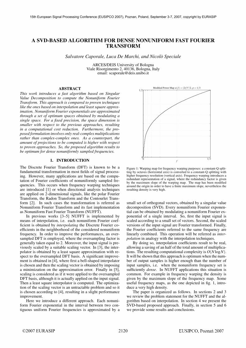
Figure 1: Warping map for frequency warping purposes: a constant-Q split-ting by octaves (horizontal axis) is converted to a constant-Q splitting withhigher frequency resolution (vertical axis). Frequency warping introduces aredundant representation of a signal, where the redundancy factor is givenby the maximum slope of the warping map. The map has been modifiedaround the origin in order to have a finite maximum slope, nevertheless theresulting density is very high.

small set of orthogonal vectors, obtained by a singular valuedecomposition (SVD). Every nonuniform Fourier exponen-tial can be obtained by modulating a nonuniform Fourier ex-ponential of a single interval. So, first the input signal isscaled according to a small set of vectors. Second, the scaledversions of the input signal are Fourier transformed. Finally,the Fourier coefficients referred to the same frequency arelinearly combined. This operation will be referred as inter-polation in analogy with the interpolation techniques.

By doing so, interpolation coefficients result to be real,allowing a saving of an half of the total amount of multiplica-tions. The resulting computational complexity is O(N logN).It will be shown that this approach is optimum when the num-ber of output samples is higher enough than the number ofinput samples, i.e. when the nonuniform frequency set issufficiently dense. In NUFFT applications this situation iscommon. For example in frequency warping the density isgiven by the maximum slope of the frequency map. Someuseful frequency maps, as the one depicted in fig. 1, intro-duce a very high density.

The paper is organized as follows. In sections 2 and 3we review the problem statement for the NUFFT and the al-gorithm based on interpolation. In section 4 we present theSVD-based proposed approach. Finally, in section 5 and 6we provide some results and conclusions.

©2007 EURASIP 2120

15th European Signal Processing Conference (EUSIPCO 2007), Poznan, Poland, September 3-7, 2007, copyright by EURASIP

47

36

24

12

0 0

12

24

36

47

10−3

10−2

10−1

100

Spectra of nonuniform Fourier exponentials.

fk n

Figure 2: Spectra of nonuniform Fourier exponentials. Nonuniform frequen-cies fk, k = 0, . . . ,K − 1, are obtained by uniformly sampling a nonlinearfunction such that f0 = 0 and fK = 1. Spectra decay slowly since periodicrepetition of a nonuniform Fourier exponential have discontinuities.

2. PROBLEM STATEMENT

Given a discrete signal xn, n = 0, . . . ,N −1, we wish to com-pute the following transformation:

X(k) =N−1

∑n=0

xne− j2π(n−τ) fk/N fk ∈ [0,N). (1)

for k = 0 . . . ,K − 1, where K is the cardinality of the setof nonuniform frequencies fk. τ is a shift parameter whichchanges the indexing of the Fourier exponentials. As partic-ular cases fk could include uniform frequencies 0, . . . ,N −1.The number of output samples K to number of input samplesN ratio will be referred as the density of the NUFFT:

ρ =K

N(2)

which will be employed in order to make considerations oncomputational complexity. The density ρ can also be in-tended as the number of different NUFFTs which must becomputed for the same input signal. The spectra of non-uniform Fourier exponentials of a particular nonuniform fre-quency map are depicted in fig. 2.

Without loss of generality, in this work we will considerthe parameter shift τ equal to N/2:

X(k) =N−1

∑n=0

xne− j2π(n−N/2) fk/N fk ∈ [0,N) (3)

since solutions to problem (1) are obtained through element

by element product between Xk and e j2π(τ−N/2) fk . The as-sumption (3) is equivalent to consider the input signal in-dexed in −N/2, . . . ,N/2− 1. In fact, signals originated bywindowing operation and images have −N/2, . . . ,N/2−1 asnatural indexing. Moreover, it will be show that this choiceallows a computational cost reduction, since in (3) the expo-nentials are nearly symmetric respect to n = N/2.

3. INTERPOLATION APPROACH

The interpolation approach is based on the on the calcula-tion of an oversampled FFT Y of the input signal scaled by asuitable vector cn:

Yi =N−1

∑n=0

cnxne− j2πni/M i = 0, . . . ,M−1 (4)

where M = mN and m ∈ N is the oversampling factor. Gen-erally m is taken equal to 2, since taking m > 2 does notincrease performances significantly. Then, the frequencyaxis is considered as a collection of M intervals [i−1/M, i),i = 0, . . . ,M−1, and nonuniform Fourier exponentials of thei-th interval are approximated by linearly combining L FFTcoefficients in the neighborhood of Yi:

X( fk) =L/2−1

∑l=−L/2

Yi+lφ( fk/m−(i+ l)) fk ∈ [i−1/m, i). (5)

This formulation is valid for even values of L, but can beeasily extended to odd values.

Clearly, (5) is an interpolation formula. So, the interpo-lating function φ must be chosen in some way. A possible ap-proach [4] consists in choosing an appropriate interpolatingcontinuous function and then finding cn so that the approxi-mation error is minimized. By doing so, φ is obtained from afinite-support bell-like function ψ by periodic repetition andphase modulation:

φ( f ) =∞

∑i=−∞

e− jπ( f−iM)(N−1)/Mψ( f − iM) (6)

and it follows:

c−1n =

∫ L/2

−L/2ψ( f )e j2π f (n−(N−1)/2)/Md f (7)

Eventually, the scaling vector can be chosen in order to makethe error result null on the oversampled Fourier frequencies0, . . . ,M−1. It follows:

c−1n =

L/2

∑l=−L/2

ψ(l)e j2πl(n−(N−1)/2)/M. (8)

Finally ψ must be chosen according to time-frequency con-siderations. It has been shown that the Kaiser-Bessel windowis a good choice for the function ψ .

From an algebraic point of view, the interpolator couldbe obtained as follows [5]. The scaling vector in (4) is as-sociated with the complex exponentials rather than with theinput signal. So, the set of the amplitude modulated Fourier

exponentials cne− j2πn(i+l)/mN , l =−L/2, . . . ,L/2−1, acts asa basis for the approximation space of nonuniform Fourierexponentials in [i−1/m, i). Then the interpolator is obtainedby a least square approach with respect to this space. Thescaling vector should be chosen in order to minimize theapproximation error. Unfortunately, an optimization overthe scaling coefficients cn is an untractable problem, so cn

are obtained by (7) or (8) according to a specified windowφ . For Kaiser-Bessel window, this algebraic approach leadsto slightly different coefficients and slightly better perfor-mances. In fig. 3 some scaled exponentials correspondingto an optimized Kaiser-Bessel interpolator are represented.

©2007 EURASIP 2121


−128 −64 0 64 127−1.5

−1

−0.5

0

0.5

1

1.5

Kaiser-Bessel scaled Fourier exponentials

Figure 3: Kaiser-Bessel scaled Fourier exponentials for N = 28, real part(solid line) and imaginary part (dotted line). In interpolation approaches,they act as basis vectors for the approximation space of nonuniform Fourierexponentials with fk ∈ [0,1/2).

4. SVD-BASED PROPOSED ALGORITHM

According to the algebraic approach described in the previ-ous section, further improvements can be achieved only byfocusing on the choice of basis vectors. In fact, thanks toscaling vector and to oversampled FFT, basis vectors of fig. 3become less regular by gaining discontinuities on the intervaledges and have slowly decaying spectra. As a consequence,the space generated by this basis achieves a better approxi-mation of nonuniform Fourier exponentials, which preciselyhave slowly decaying spectra, as depicted in fig. 2. So, inorder to obtain an optimum approximation, we want to findan optimum basis.

In the present section we will use a matrix notation.Taken a generic operator A, the adjoint and the transpose op-erators will be represented by A† and A′ respectively. Themeaning of subscripts and superscripts will be specified atany time they are used. A vector of generic size N willbe indexed in 0, . . . N − 1. Indexes which are not includedin 0, . . . , N − 1 are to be intended as modN . The symbolsδ0,δ1 δ2, . . ., will denote shifted impulsive column vectors ofsuitable size.

First, we define the following unitary operators:

T = [δ1 δ2 · · · δN−1 δ0] (9)

R = [δN−1 δN−2 · · · δ1 δ0] (10)

which represent circular shift and time-reversing respec-tively. Now we consider the [N×K] matrix E whose columnsare nonuniform Fourier exponentials. The elements E(n,k)of this matrix are given by:

E(n,k) = e j2π(n−N/2) fk/N . (11)

Thanks to the considered time indexing, the real part of thecolumns of E is symmetric and the imaginary part is anti-symmetric with respect to n = N/2, apart for n = 0:

E = ZE∗ + j2δ0δ ′

0 ℑ[E]

where δ0δ ′

0 is a two-dimensional impulsive [N ×N] matrix

0

0.125

0.25

.375

0.5 0

64

128

192

255

−1

−0.5

0

0.5

1

Inverse Fourier Transforms of nonuniform Fourier exponentials

fk n

Figure 4: Entries of the matrix F†E0. When nonuniform frequency fk tends

to 0, the matrix column tends to be an impulse. The columns are very cor-related, so the rank of the matrix is small.

and Z is defined as follows:

Z = TR = [δ0 δN−1 · · · δ2 δ1]. (12)

The operator Z acts as a complex conjugation only if it is ap-plied to the Fourier transform of a real vector, so F†E is realif ℑ[E(0, ·)] = 0, where F represents the Fourier transform.In order to deal with a real matrix rather than with a complexone, we introduce the following operator:

E = E− jδ0δ ′

0 ℑ[E]. (13)

By defining the row vector D = jℑ[E(0, ·)] of size K, thecolumn vector X of size K representing the NUFFT (3) ofthe input signal x results:

X = E†x = E†x+D†x0. (14)

Now, the nonuniform frequency set is partitioned in 2Nsubsets corresponding to contiguous frequency intervals:

f(l)k ∈ [l/2, l/2+1/2) l = 0, . . . ,2N −1 (15)

whose cardinalities are Kl . Then, the set of nonuniformFourier exponentials corresponding to each interval is con-sidered:

El(n,k) = e j2π(n−N/2) f(l)k

/N (16)

It is worth to note that El , for even l, could be obtained bymodulating the column vectors of a nonuniform Fourier ma-trix referred to a suitable set of frequencies fk ∈ [0,1/2),which will be represented as El,0. For odd l, El could beobtained in the same way from a nonuniform Fourier matrixwhose frequencies refer to fk ∈ [−1/2,0), which could bealso obtained by conjugating a suitable matrix El,0. Mod-ulation can be converted in circular shift by passing in theFourier domain, so, by some some calculations, it follows:

El = (−1)iFT−iF†El,0 l = 2i (17)

El = (−1)iFT−iF†E∗

l,0R l = 2i−1. (18)

©2007 EURASIP 2122


where the formulation (14) has been exploited in order to

deal with the real matrixes F†El,0. In general, each matrix

El,0 refers to randomly distributed frequencies in [0,1/2).In order to find a single basis for the column vectors of all

matrixes El,0, we can equally consider a generic matrix E0

which ideally has as column vectors every possible nonuni-form Fourier exponentials in [0,1/2). In practice, it suf-fices to consider a finite set of nonuniform frequencies whichdensely cover the whole [0,1/2) interval. This matrix hasvery correlated column vectors, as depicted in fig. 4, so itsrank results to be small for a certain precision. As a conse-quence, a singular value decomposition can be introduced,

i.e. F†E0 = USV′. The singular values decay exponentially,so we could consider a reduced number L of singular valuesand neglect the others:

F†E0 ≃ ULSLV′

L (19)

where UL and VL are constituted by the first L columns of Uand V respectively and SL is a square matrix constituted bythe first L rows and columns of S. The column vectors of UL

represent an optimum basis for all the matrixes E0,l . Then,

the decomposition is extended to El in the following way:

El ≃ FT−iULP′

l l = 2i (20)

El ≃ FT−iZULP′

l l = 2i−1 (21)

where each Pl is a real [Kl ×L] matrix which linearly com-bine the column vectors of UL in order to obtain the bestapproximation of El,0. Since UL has orthogonal columns, Pl

are simply obtained by computing:

Pl = (TiF†El)′UL l = 2i (22)

Pl = (ZTiF†El)′UL l = 2i−1. (23)

The column vectors of each El are approximated by linearlycombining the columns of FT−iUL or FT−iZUL through therows of the matrix Pl . In order to compute (14), we mustcalculate the scalar products between x and the columns ofFT−iUL and FT−iZUL in an efficient way. With some al-gebra, it has been found that first, x must be scaled by theFourier antitrasformed vectors of UL, W = F†UL:

X = diag(x)W (24)

where diag(x) is a matrix having x as main diagonal. Thecolumns of W corresponding to the first 6 singular values aredepicted in fig. 5. Then, the Fourier transforms of the columnvectors of X produce the needed N ×L scalar products:

Q = FX (25)

Each row of Q will be pointed by Qi. Finally we obtain that

X (l) = E†l x is given by the product between a [Kl ×L] matrix

and a column vector of size L:

X (l)≃ PlQ

†i l = 2i (26)

X (l)≃ PlQ

′

−i l = 2i−1 (27)

Summarizing, the algorithm consists in precomputing inter-polation coefficients (22)-(23), computing L scaling (24),calculating N×L scalar products (25) and interpolating them(26)-(27). It is worth to note that the term interpolation isonly used in analogy with the conventional technique.

−128 −64 0 64 127

−0.1

−0.05

0

0.05

0.1

SVD-approach basis vectors

Figure 5: Fourier Transforms of the first 6 orthogonal vectors UL, real part(solid line) and imaginary part (dotted line). These vectors have the samerole which vectors depicted in fig. 3 play in the conventional approach.

5. PERFORMANCES

The computational cost of both interpolation and SVD-basedapproaches is given by three terms, cost of scaling, cost ofFourier transforms and cost of interpolation. In terms of realmultiplication, for the presented algorithm it results:

κsvd = 2LN +4LN log2 N +2LNρ (28)

where ρ represents the NUFFT density (2). The first additiveterm derives from (24), where L element-by-element prod-ucts between a real and a complex vector of size N are com-puted, i.e. 2LN real multiplications. The second term derivesfrom (25), where L Fourier transforms of vectors of size Nare computed. Each Fourier transform needs 4N log2 N realmultiplications. Finally, the third term derives from (26)-(27)where K = ρN scalar products between a real and a complexvector of size L are computed, or, equally, L complex scalingof a real vector of size ρN. The cost of D†x0 (14) can be ne-glected. Through analogous considerations, for interpolationtechniques it results:

κint = N +8N log2 N +4LNρλ . (29)

The factor λ > 1 is an effective parameter which takes intoaccount that, for the same value of L, SVD-based approachhas better performances, as depicted in fig. 6. For useful val-ues of L, λ is nearly equal to 1,4. As far as memory re-quirements are concerned, in terms of real numbers for theSVD-approach it results:

µsvd = LN +LNρ +Nρ (30)

where terms correspond to the complex vectors W to the realinterpolation coefficients Pl and to the vector D respectively.Only LN real coefficients are necessary for the vectors W,since they are the Fourier transforms of the real vectors UL.Similarly, for interpolation approach it results:

µint = N +2LNρλ . (31)

©2007 EURASIP 2123


2 4 6 8 10 12 14 16

10−13

10−11

10−9

10−7

10−5

10−3

10−1

Approximation error vs size L of the interpolator

Interpolation

SVD

Figure 6: Comparison between the approximation errors given by the pro-posed SVD-based and the interpolation algorithm versus the size of the in-terpolator. The maximum of the euclidian norm of the error have beenmeasured.

0

0.125

0.25

0.375

0.5 0

64

128

192

255

10−9

10−7

10−5

fkn

(a) Approximation error of E0 by interpolation approach, L = 8

0

0.125

0.25

0.375

0.5 0

64

128

192

255

10−12

10−10

10−8

fkn

(b) Approximation error of E0 by SVD-based approach, L = 8

Figure 7: Comparison between the approximation errors of the matrix E0

given by the interpolation approach (a) and the proposed SVD-based ap-proach (b), for size L of the interpolator equal to 8.

A fair comparison between the two approaches is quitehard. Sufficient conditions for SVD-approach to be less ex-pensive than interpolation approach are:

ρ > log2 N ⇒ κsvd < κint (32)

ρ > 1 ⇒ µsvd < µint (33)

In worst cases, when ρ ≈ 1, the proposed method would con-sist in more multiplications because of the computation of LFourier transforms. Nevertheless, the algorithm has a serialstructure, since each basis vector requires the computation ofa scaling, a fast Fourier transform and its contribution to theinterpolation, which is actually another scaling. Moreover, itdoes not involve complex multiplications in the scaling andinterpolation computation. Furthermore, since the algorithmis based on orthogonal projections, the size of the interpola-tor L can be increased by simply adding basis vectors. Fi-nally, the fast Fourier transform, being a very common op-eration, is generally optimized and efficiently managed. Forthese reasons, the comparison have been focused only on theapproximation error respect to the size L of the interpolatoremployed to approximate each nonuniform Fourier exponen-tial, represented in fig. 6. In fig. 7 we have compared theapproximation errors for a generic matrix E0, i.e. a matrixwith nonuniform frequencies in [0,1/2) for interpolator sizeL equal to 8. The error given by SVD-based approach is 3orders of magnitude lower than error given by interpolationapproach, in coherence with values represented in fig. 6.

6. CONCLUSIONS

In this work we presented a novel approach for the computa-tion of the Nonuniform Fourier Transform based on SingularValue Decomposition. The proposed algorithm has quasi-linear complexity. In comparison with the conventional in-terpolation approach, our proposed approach has been shownto have a higher computational cost for the calculation ofthe projection components, but a lower cost for interpolat-ing them. Moreover, this algorithm provides advantages interms of computational structure, being based on Fast FourierTransforms and real multiplications.

REFERENCES

[1] S. Caporale, L. De Marchi, and N. Speciale, “An ac-curate algorithm for fast frequency warping,” in Proc.IEEE International Symposium on Circuits and Systems,2007, pp. 1811–1814.

[2] M.N. Do and M. Vetterli, “The contourlet transform:an efficient directional multiresolution image represen-tation,” IEEE Trans. Image Processing, vol. 14, no. 12,pp. 2091–2106, 2005.

[3] Q.H. Liu and N. Nguyen, “The regular Fourier matricesand nonuniform fast Fourier transforms,” SIAM Journalon Scientific Computing, vol. 21, no. 1, pp. 283–293, Jan.1999.

[4] A. Dutt and V. Rokhlin, “Fast fourier transforms fornonequispaced data,” SIAM Journal on Scientific Com-puting, vol. 14, no. 6, pp. 1368–1393, 1993.

[5] J.A. Fessler and B.P. Sutton, “Nonuniform fast fouriertransforms using min-max interpolation,” IEEE Trans.Signal Processing, vol. 51, no. 2, pp. 560–574, 2003.

©2007 EURASIP 2124


Documents

A SVD-Based Algorithm for Dense Nonuniform Fast Fourier