Embed Size (px)
Citation preview
A Survey on Visualization of Time-Dependent Vector Fields
by Texture-based Methods
Henry “Dan” DerbesMSIM 842 ODU Main Campus
Outline
• Introduction – motivation, background terms
• Fundamental texture based methods o Spot Noiseo Line Integral Convolution (LIC)
• Unsteady flow methods o Unsteady Flow LIC (UFLIC)o Dynamic LIC (DLIC)o Lagrangian-Euler Advection (LEA)o Image Base Flow Visualization (IBFV)o Unsteady Flow Advection-Convolution (UFAC)
Motivation• Survey goal: Explore ideas that led to techniques for
using texture and dye to visualize unsteady vector fields in 3D
• Visualization of scalar and vector fields associated with flow over surfaces has many applications o Common scalar functions of two variables o 3D distribution of pressure and velocity over a ship hull or
airplane wings
• Common goal: produce high-resolution images that reveal flow field characteristics o Orientation o Direction o Magnitude o Rate of change
Background
• Spatial resolution of the vector field: o Sampling with stream lines or particle traceso Icons at every vector field coordinate
• Problem: these techniques depend critically on placemento Eddies or currents can be missed o Icons do not miss data but use up a lot of spatial resolution
• Time-dependent methods progressively track visualization results over time
• To achieve coherent animations, continuously track visualization objects such as particles over time
Texture-based methods
• Texture-based methods offer higher resolution outputs than previous approaches o Vector plots o Particle tracing o Stream surfaces o Volume rendering
Terms
• Advection is the transport of a fluid
• Convolution is a mathematical operator which takes two functions and produces a third function
• Volume rendering creates a 2D image from scalar or vector datasets of multiple dimensions
• Particle tracing techniques place a set of insertion points into a flow field. Particles are released from the insertion points to trace the flow pattern
• Streamlines are tangent to a vector field at every point
Terms
• Pathlines trace the trajectory of individual particles
• Streaklines are the traces of a set of particles emitted from the same insertion points
• Timelines link the particles emitted at the same time from different insertion points.
Pathlines, Streaklines, Streamlines are identical for steady flows.
Spot Noise
• In 1991,van Wijk proposed “spot noise”o Texture is synthesized by addition of
randomly weighted and positioned spots. o Local control is achieved by variation of the
spot. o The spot is a useful primitive for texture
design, because the relationship between spot and texture features is generally straightforward.
Spot Noise
• van Wijk developed a convolution with a white noise texture. Texture synthesis occurs in two steps: o Data corresponding to texture coordinates are
retrieved. o Data are converted to parameter values using a
mapping scheme which expresses the variation.
• Spot noise is synthesized through the convolution of a white noise grid and the spot.
Spot Noise
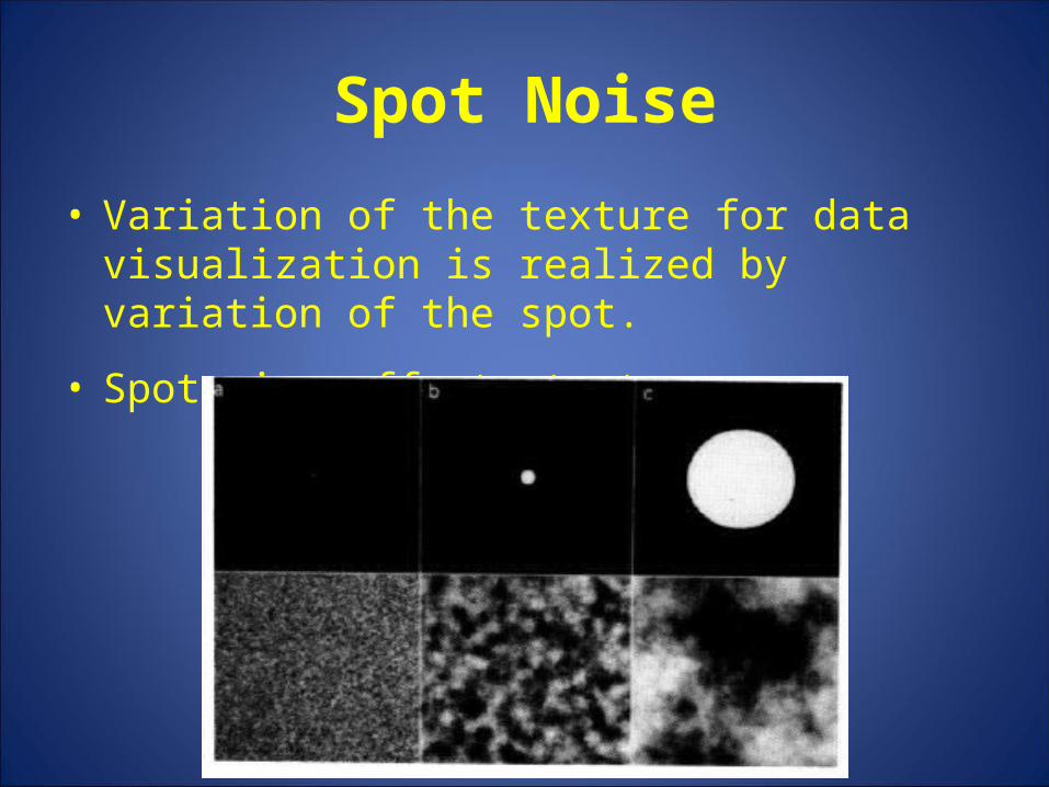
• Variation of the texture for data visualization is realized by variation of the spot.
• Spot size affects texture
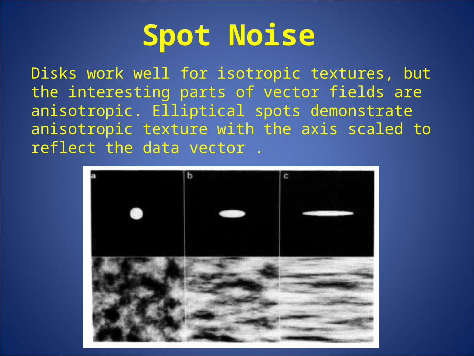
Spot Noise Disks work well for isotropic textures, but the interesting parts of vector fields are anisotropic. Elliptical spots demonstrate anisotropic texture with the axis scaled to reflect the data vector .
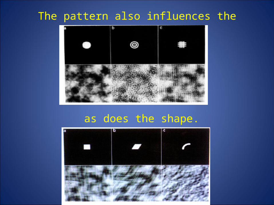
The pattern also influences the texture
as does the shape.
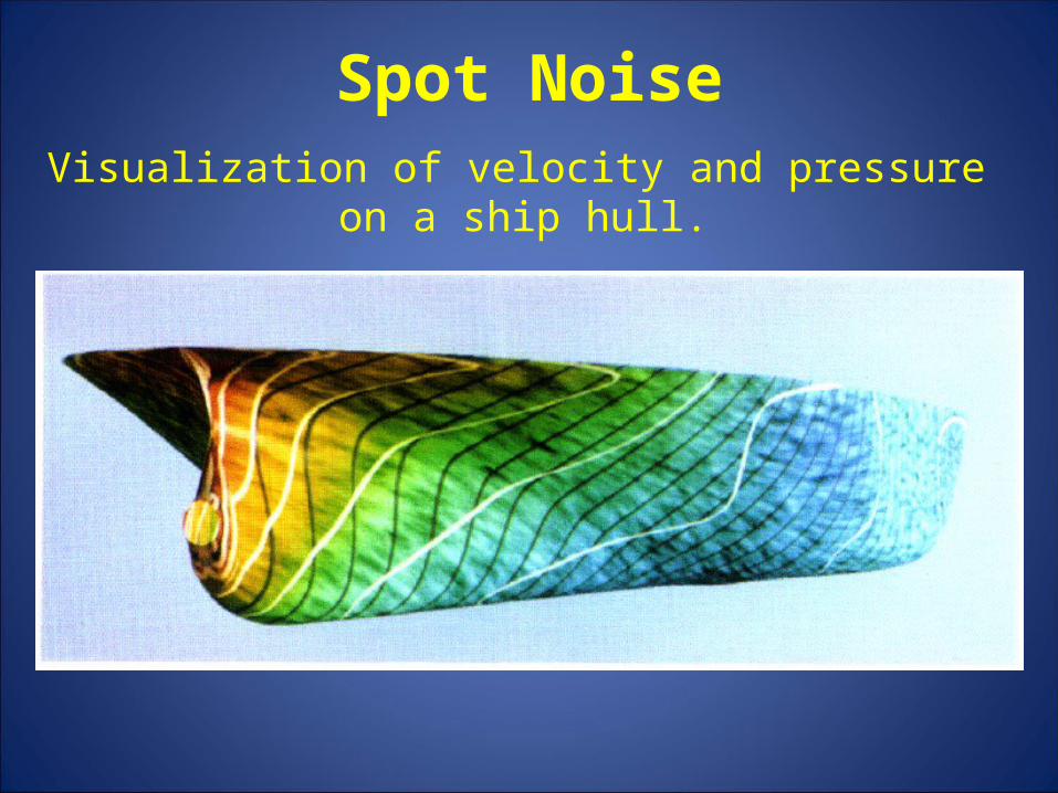
Spot NoiseVisualization of velocity and pressure on a ship hull.
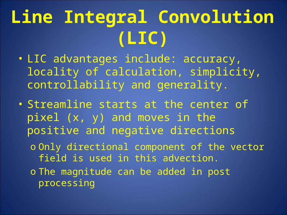
Line Integral Convolution (LIC)
• LIC advantages include: accuracy, locality of calculation, simplicity, controllability and generality.
• Streamline starts at the center of pixel (x, y) and moves in the positive and negative directions o Only directional component of the vector field is
used in this advection. o The magnitude can be added in post processing
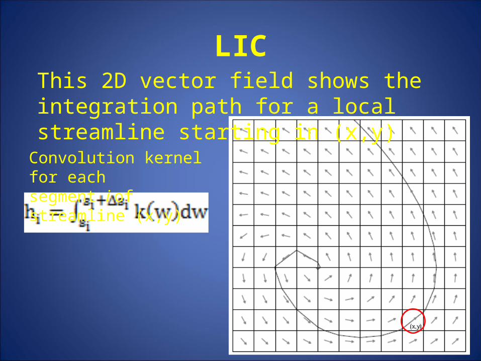
LICThis 2D vector field shows the integration path for a local streamline starting in (x,y)
Convolution kernel for eachsegment i of streamline (x,y)
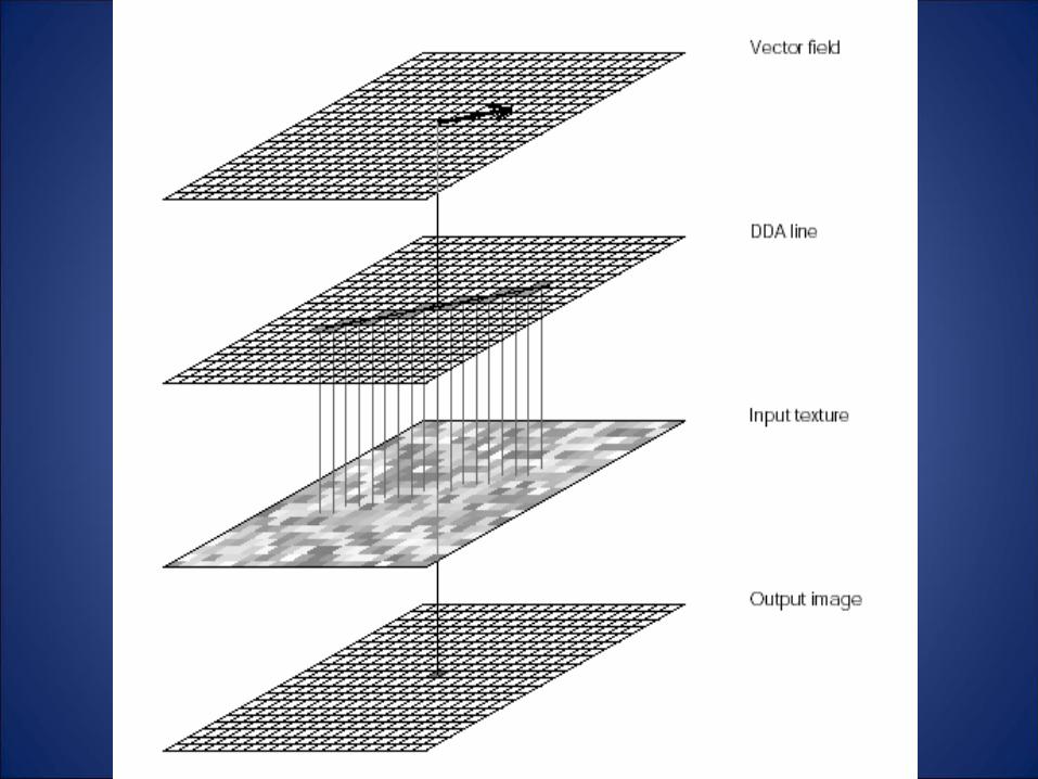
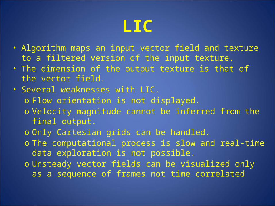
LIC• Algorithm maps an input vector field and texture to a filtered
version of the input texture. • The dimension of the output texture is that of the vector
field. • Several weaknesses with LIC.
o Flow orientation is not displayed. o Velocity magnitude cannot be inferred from the final
output.o Only Cartesian grids can be handled.o The computational process is slow and real-time data
exploration is not possible.o Unsteady vector fields can be visualized only as a
sequence of frames not time correlated
Unsteady Flow LIC (UFLIC)
• Simulates the advection of flow traces globally in unsteady flow fields.
• White noise input texture advected over time to create directional patterns of the flow at every time step.
• Convolution method is called time-accurate value scattering scheme. o Image value at every pixel is scattered forward following the
flow’s pathline trace o Image value has a time stamp and particle have short lifespano Time-accurate value scattering process is repeated at every
time step. • The resulting texture from the previous convolution step
is used to compute the new convolution after performing high-pass filtering.
• Method acts as a low-pass filter diminishing contract
Unsteady Flow LIC (UFLIC)
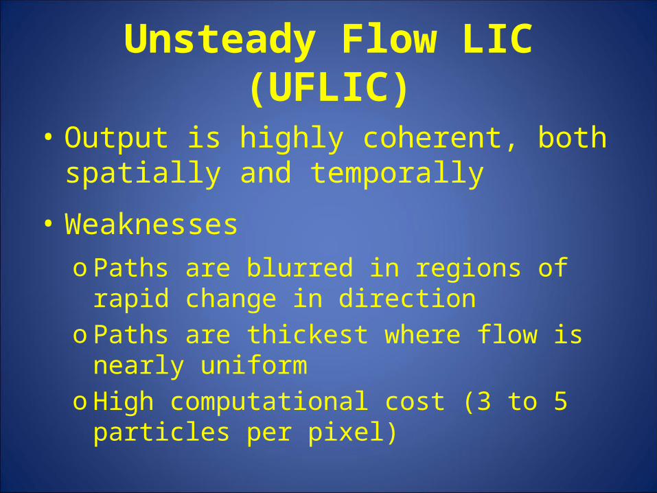
• Output is highly coherent, both spatially and temporally
• Weaknesseso Paths are blurred in regions of rapid change
in directiono Paths are thickest where flow is nearly
uniformoHigh computational cost (3 to 5 particles per
pixel)
Dynamic LIC (DLIC)
• Has the outstanding resolution of LIC but is able to generate animation sequences of time-varying fields with temporal coherence.
• Extends LIC to time-dependent fields making it possible to visualize the evolution of streamlines.
• The vector field varies arbitrarily over time with the motion of streamlines describes by a second “motion” vector field.
• Each frame is rendered using LIC.
• The input texture is generated by advecting a dense collection of particles over time and adjusting them to maintain the appropriate level of detail.
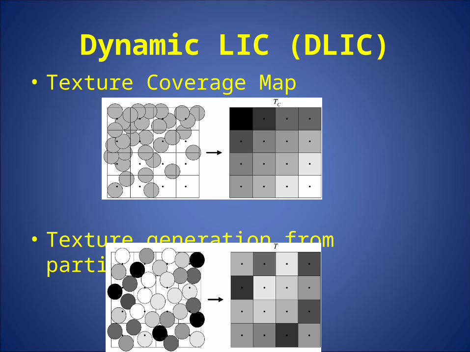
Dynamic LIC (DLIC)• Texture Coverage Map
• Texture generation from particles
Lagrangian-Eulerian Advection (LEA)
• Motion of a dense collection of particles (one per pixel)• High spatio-temporal correlation• Interactive frame rates through spatial locality and
instruction pipelining• Lagrangian approach: the trajectory of each particle is
computed separately. • Eulerian approach: particles lose their identity however,
the particle property, viewed as a field, is known for all time at any spatial coordinate.
• LEA is a hybrid method. For each time step:– Particle coordinates are calculated through Lagrangian
integration– Advection of particle property through an Eulerian method
Lagrangian-Eulerian Advection (LEA)
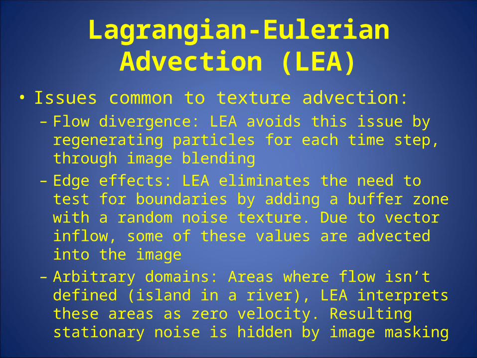
• Issues common to texture advection:– Flow divergence: LEA avoids this issue by
regenerating particles for each time step, through image blending
– Edge effects: LEA eliminates the need to test for boundaries by adding a buffer zone with a random noise texture. Due to vector inflow, some of these values are advected into the image
– Arbitrary domains: Areas where flow isn’t defined (island in a river), LEA interprets these areas as zero velocity. Resulting stationary noise is hidden by image masking
Lagrangian-Eulerian Advection (LEA)
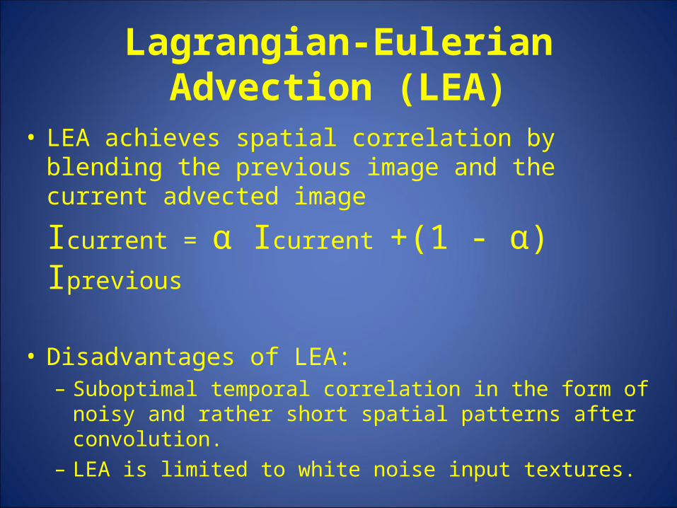
• LEA achieves spatial correlation by blending the previous image and the current advected image
Icurrent = α Icurrent +(1 - α) Iprevious
• Disadvantages of LEA: – Suboptimal temporal correlation in the form of noisy
and rather short spatial patterns after convolution. – LEA is limited to white noise input textures.
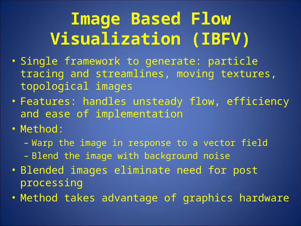
Image Based Flow Visualization (IBFV)
• Single framework to generate: particle tracing and streamlines, moving textures, topological images
• Features: handles unsteady flow, efficiency and ease of implementation
• Method:– Warp the image in response to a vector field– Blend the image with background noise
• Blended images eliminate need for post processing
• Method takes advantage of graphics hardware
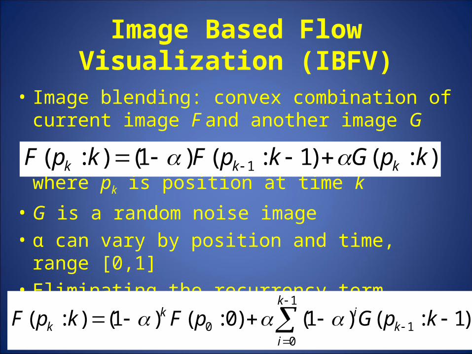
Image Based Flow Visualization (IBFV)
• Image blending: convex combination of current image F and another image G
where pk is position at time k
• G is a random noise image
• α can vary by position and time, range [0,1]
• Eliminating the recurrency term gives:
):()1:()1():( 1 kpGkpFkpF kkk
)1:()1()0:()1():( 1
1
00
kpGpFkpF k
k
i
ikk
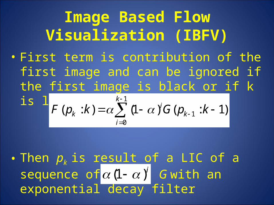
Image Based Flow Visualization (IBFV)
• First term is contribution of the first image and can be ignored if the first image is black or if k is large.
• Then pk is result of a LIC of a sequence of images G with an exponential decay filter
)1:()1():( 1
1
0
kpGkpF k
k
i
ik
i)1(
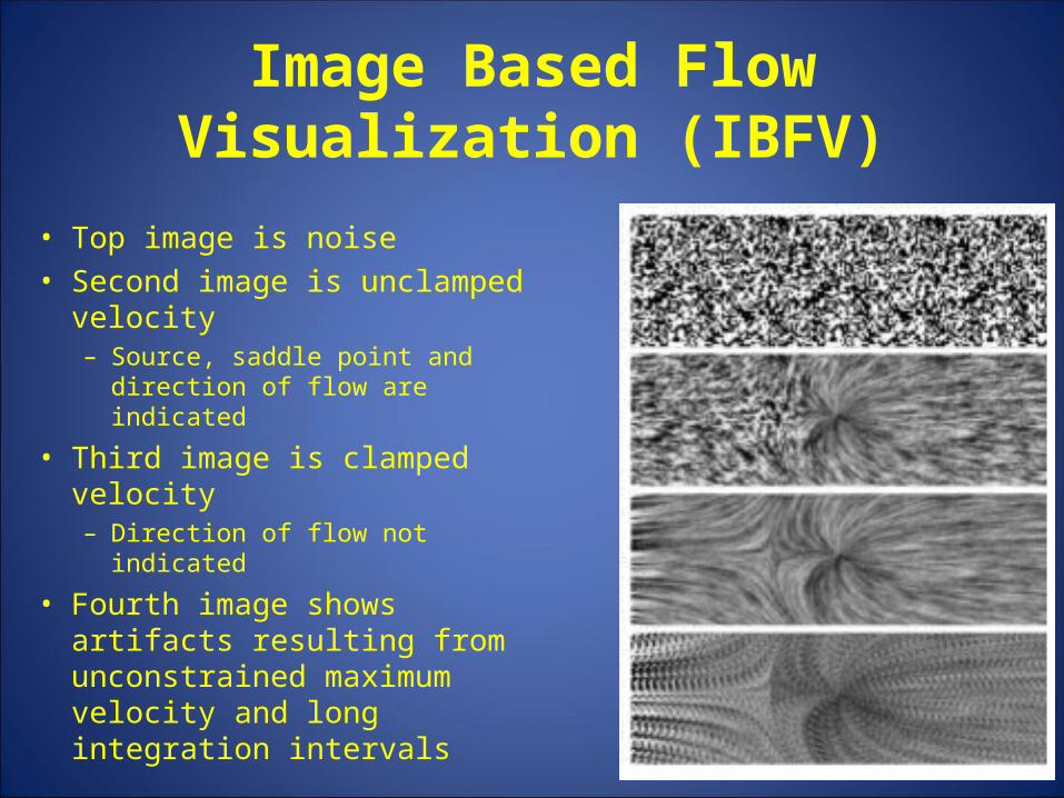
Image Based Flow Visualization (IBFV)
• Top image is noise• Second image is unclamped
velocity– Source, saddle point and direction
of flow are indicated
• Third image is clamped velocity– Direction of flow not indicated
• Fourth image shows artifacts resulting from unconstrained maximum velocity and long integration intervals
Unsteady Flow Advection-Convolution (UFAC)
• Provides the user with separate control over temporal and spatial coherence – Allows use of more advanced visualization techniques
• Dense representation of time-dependent vector field• Takes white noise, filtered noise, color as texture input• Method:
– First, continuous trajectories are constructed in spacetime to guarantee temporal coherence.
• Performs time evolution of unsteady fluid flows using pathlines
– Second, convolutions along another set of paths through the above spacetime result in spatially correlated patterns.
• Builds spatial correlation according to instantaneous streamlines.
• Length of the streamlines is related to the degree of unsteadiness of the vector field.
Unsteady Flow Advection-Convolution (UFAC)
• A texture-based approach:– Spatial slices of the property field are constructed from trajectories– Trajectories for each texel backward in time are iteratively computed
using Lagrangian methods– Combine spatial slices to build the spacetime domain– Compute a convolution along each pathline in the 3D property field
• Particles have limited lifetime
• Common Issues– Edge effects: input texture is larger than output creating a boundary
region– Divergence: limited lifespan of particles, continuous injection of new
particles– Arbitrary domains: not addressed
Unsteady Flow Advection-Convolution (UFAC)
• UFAC cannot solve the fundamental dilemma of inconsistency between spatial and temporal patterns, but it explicitly addresses the problem and directly controls the length of the spatial structures. It maximizes the length of spatial patterns and the density of their representation while retaining temporal coherence.
Conclusion
• Texture based methods support visualization of complex dynamic fluid flows
• Interactive visualizations have been demonstrated but need to continue to improve
• Display of 3D dynamic vector fields has much room for development– Sparse representations– Semi-transparency– Feature extraction