Embed Size (px)
Citation preview

A Survey of Strategies on Prolonging
the Lifetime of Sensor Networks
Yibo Sun
University of SUNY Binghamton
Abstract
The lifetime of wireless sensor network is crucial, since autonomous operation must be
guaranteed over an extended period. In most sensor network applications, all the sensor data
has to be forwarded to the only sink via multi-hop routing, the traffic pattern is thus highly
nonuniform, putting a high burden on the sensor nodes close to the observer.
In this paper, we define the lifetime of sensor network in application oriented way, analyze the
energy optimization effort and energy balancing strategies on routing protocols, and finally
we describe an application oriented optimization strategy.
I.... Introduction
Rapid commoditization and increasing integration of micro-sensors, digital signal processing
and low-range radio electronics on a single node has lead to the idea of distributed, wireless
networks that have the potential to collect data more cost effectively, autonomously and
robustly compared to a few macro-sensors. Applications of such massively distributed sensor
networks include seismic, acoustic, medical and intelligence data gathering and fire, climate,
equipment monitoring etc.
One main factor which make wireless sensor networks differ from other types of multi-hop
wireless networks is that in most cases a sensor node is highly power constrained, for
example, powered by battery. Hence one of the most difficult challenges is to prolong the life
time of the sensor network, which directly determines the duration of the sensing task.
Three general ideas exist in the design of energy efficient sensor networks, i.e., how to reduce
the total energy consumption on the whole network, how to transmit data packets efficiently,
and how to balance the energy on sensor nodes. In this paper, we assume that transmit a data
packet to a neighbor node is a constant value; hence we will mainly discuss the first and the
last idea and the related work.
There are a lot of factors which affect the network lifetime, sensing field, node capability (e.g.
homogenous or heterogeneous), location knowledge, radio coverage, deployment strategy (e.g.
random deployment, regular geometric topology, or planned deployment) , routing protocol,
etc. This paper will mainly focus on the factor of routing protocol. Some prior researches
show that sending or receiving a bit of message consumes about 1000 times of compute on it,
hence we may take the total number of received and sent packets to measure the energy
consumed.
The rest of this paper will organize as follows. In part II, we will review some definitions of
lifetime of sensor networks and give an application oriented version. In part III, we will give
out the energy consumption model and provide a comparison of lifetime in 3 most general

topologies, direct communication, minimum transmission energy (multi-hop), and clustering.
In part IV, we will review the former effort on maximizing the network lifetime from
hop-to-hop, end-to-end and in whole picture. In part V, we will propose an application
oriented optimization strategy.
II.... DEFINITION OF NETWORK LIFETIME
2.1 Problem Definition
Consider the case in figure 1 that all the sensor nodes are static and modeled as an undirected
graph G(V, L), where V is the number of nodes, |V| = n, and L is the set of links. Each node
has initial capacity Bi, and needs to communicate with the sink node at rate Si. The node
lifetime of node i under flow r = {rij} is given by ∑ ∈
=ijijNj
ii
rE
BrT
i
)( [8]
where Ni = {j| (i, j)∈L}
Figure 1
While a formal definition of network lifetime is not straightforward and may depend on the
application scenario in which the network is used. Network lifetime can be defined as the
time for the last node to die. An example for this kind of application can be tracing for a
criminal. Micro sensors are hided on a suspect’s clothes, shoes, etc., some for reporting the
position and some for reporting the height. As long as one sensor alive, the network is
functioning.
Alternatively, network lifetime has been defined as the time for the first node to die by
)(min)( rTrT iVi
net ∈= [8][3], or as the time for a certain percentage of network nodes to die.
For example, in Figure 2, let the node#1 is the only sink, and all the data will transmit
through node#6, which will quickly runs out of power and cause the network out of
functioning. And the network lifetime has been defined in terms of the packet delivery rate or
in terms of the number of alive flows[4], thus accounting the alive nodes for achieving the
“quality of communication”.
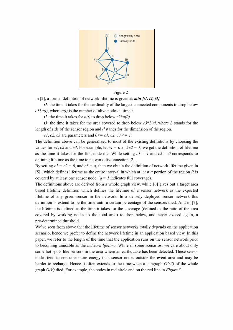
Figure 2
In [2], a formal definition of network lifetime is given as min {t1, t2, t3}.
t1: the time it takes for the cardinality of the largest connected components to drop below
c1*n(t), where n(t) is the number of alive nodes at time t.
t2: the time it takes for n(t) to drop below c2*n(0)
t3: the time it takes for the area covered to drop below c3*L^d, where L stands for the
length of side of the sensor region and d stands for the dimension of the region.
c1, c2, c3 are parameters and 0<= c1, c2, c3 <= 1.
The definition above can be generalized to most of the existing definitions by choosing the
values for c1, c2 and c3. For example, let c1 = 0 and c2 = 1, we get the definition of lifetime
as the time it takes for the first node die. While setting c1 = 1 and c2 = 0 corresponds to
defining lifetime as the time to network disconnection [2].
By setting c1 = c2 = 0, and c3 = q, then we obtain the definition of network lifetime given in
[5] , which defines lifetime as the entire interval in which at least q portion of the region R is
covered by at least one sensor node. (q = 1 indicates full coverage).
The definitions above are derived from a whole graph view, while [6] gives out a target area
based lifetime definition which defines the lifetime of a sensor network as the expected
lifetime of any given sensor in the network. In a densely deployed sensor network this
definition is extend to be the time until a certain percentage of the sensors died. And in [7],
the lifetime is defined as the time it takes for the coverage (defined as the ratio of the area
covered by working nodes to the total area) to drop below, and never exceed again, a
pre-determined threshold.
We’ve seen from above that the lifetime of sensor networks totally depends on the application
scenario, hence we prefer to define the network lifetime in an application based view. In this
paper, we refer to the length of the time that the application runs on the sensor network prior
to becoming unusable as the network lifetime. While in some scenarios, we care about only
some hot spots like sensors in the area where an earthquake has been detected. These sensor
nodes tend to consume more energy than sensor nodes outside the event area and may be
harder to recharge. Hence it often extends to the time when a subgraph G’(V) of the whole
graph G(V) died, For example, the nodes in red circle and on the red line in Figure 3.

Figure 3
III.... AN COMPARISON ON LIFETIME IN DIFFERENT
TOPOLOTIES
3.1 The Energy Consumption Model
A micro sensor has three core components which are radio transceiver, micro controller and
energy source. In this paper, we only consider the energy consumed by sending and receiving
data packets, showed in figure 4 [9]. In fixed transmit radio power level, energy used to
send/receive one bit is bitnJEelec /50= , and 2//100 mbitpJamp =ε . Hence transmitting a
k-bit packet a distance d costs 2
) *),()(,( dkkEdkEkEdkE electxamptxelectx ∗∗+=+= ε , and
the energy consumed in receiving it is kEkEkE elecrxelecrx *)(( ) == . We choose 2 as the
propagation parameter while in real propagation model, E = k*dc, 2<c<4.
Figure 4
3.2 Topologies Compared
Direct communication is the simplest topology where all sensor nodes are one hop away from
the base station, see figure5. Each sensor node sends its data directly to the base station; hence
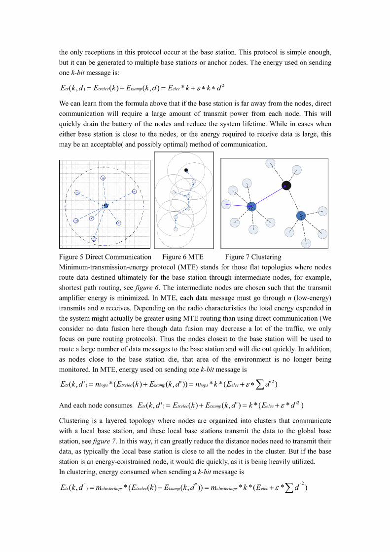
the only receptions in this protocol occur at the base station. This protocol is simple enough,
but it can be generated to multiple base stations or anchor nodes. The energy used on sending
one k-bit message is:
2) *),()(,( dkkEdkEkEdkE electxamptxelectx ∗∗+=+= ε
We can learn from the formula above that if the base station is far away from the nodes, direct
communication will require a large amount of transmit power from each node. This will
quickly drain the battery of the nodes and reduce the system lifetime. While in cases when
either base station is close to the nodes, or the energy required to receive data is large, this
may be an acceptable( and possibly optimal) method of communication.
Figure 5 Direct Communication Figure 6 MTE Figure 7 Clustering
Minimum-transmission-energy protocol (MTE) stands for those flat topologies where nodes
route data destined ultimately for the base station through intermediate nodes, for example,
shortest path routing, see figure 6. The intermediate nodes are chosen such that the transmit
amplifier energy is minimized. In MTE, each data message must go through n (low-energy)
transmits and n receives. Depending on the radio characteristics the total energy expended in
the system might actually be greater using MTE routing than using direct communication (We
consider no data fusion here though data fusion may decrease a lot of the traffic, we only
focus on pure routing protocols). Thus the nodes closest to the base station will be used to
route a large number of data messages to the base station and will die out quickly. In addition,
as nodes close to the base station die, that area of the environment is no longer being
monitored. In MTE, energy used on sending one k-bit message is
)'(**))',()((*',( 2) ∑∗+=+= dEkndkEkEndkE elechopstxamptxelechopstx ε
And each node consumes )'*(*)',()(',( 2) dEkdkEkEdkE electxamptxelectx ε+=+=
Clustering is a layered topology where nodes are organized into clusters that communicate
with a local base station, and these local base stations transmit the data to the global base
station, see figure 7. In this way, it can greatly reduce the distance nodes need to transmit their
data, as typically the local base station is close to all the nodes in the cluster. But if the base
station is an energy-constrained node, it would die quickly, as it is being heavily utilized.
In clustering, energy consumed when sending a k-bit message is
)*(**)),()((*,(2''''
)'' ∑+=+= dEkmdkEkEmdkE elecsclusterhoptxamptxelecsclusterhoptx ε

And each node will consume )*(*),()(,(2''''
)'' dEkdkEkEdkE electxamptxelectx ε+=+= .
3.3 Experimental Results [9]
Figure 8 below shows the number of living nodes per time past. We can learn that the nodes
die out quicker using MTE routing than direct transmission while the last node live longer
than direct communication which prove the result of the formula analysis. Clustering with
static power constrained cluster heads even do worse for after the death of cluster heads, the
whole network are divided into small areas which are disconnected.
Figure 8 Direct vs. MTE vs. Static Clustering Figure 9 Direct vs. MTE vs SC vs Leach
From the
Figure 8 Direct vs. MTE vs. Static Clustering
Compare “the round first node dies” and “the round last node dies” in figure 9, we can see
that the lifetime of sensor nodes are in a big range. The application will out of functioning
long before the last node dies.
Figure 9 Direct vs. MTE vs. Static Clustering vs. LEACH
IV.... ENERGY AWARING ROUTING
4.1 End-to-End Optimization Routing
a. Minimum Total Transmission Power Routing (MTPR) [10]
The main idea of MTPR is to reduce the total transmission power per packet. It will calculate
the energy needed along all possible routes as ∑−
=+=
1
0
1),()(d
i
iid nnTrP , and choose the
optimal route )(min)( jo rPrP = . And hence MTPR prefers routes with more hops with
short transmission ranges than few hops with longer transmission range. The problem is it
will cost more extra energy, cause a big delay and not scalable.
b. Min-Max Battery Cost Routing (MMBCR)
MMBCR consider the remaining batter power of nodes )(/1)( tctf ii = as metric. In made
route option, MMBCR will pick up the minimum value of battery power on each possible
route )(max)( tfrR ij = and then choose the maximum one, )(min)( jo rRrR = . MMBCR
prefer to choose a path whose weakest node has the maximum remaining power. Hence nodes
with high residual capacity participate in routing more often. MMBCR suffers the same delay
and scalability problem as MTPR.
c. Conditional Min-Max Battery Cost Routing (CMMBCR)
CMMBCR is based on MMBCR. It set a parameter γ as threshold, if no node in the chosen
route with MMBCR algorithm whose battery capacity is lower than γ , MMBCR applied, else,
MTPR applied.
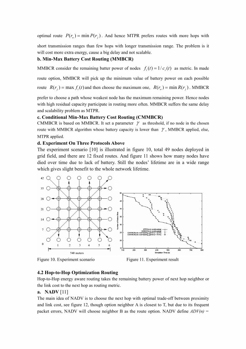
d. Experiment On Three Protocols Above
The experiment scenario [10] is illustrated in figure 10, total 49 nodes deployed in
grid field, and there are 12 fixed routes. And figure 11 shows how many nodes have
died over time due to lack of battery. Still the nodes’ lifetime are in a wide range
which gives slight benefit to the whole network lifetime.
Figure 10. Experiment scenario Figure 11. Experiment result
4.2 Hop-to-Hop Optimization Routing
Hop-to-Hop energy aware routing takes the remaining battery power of next hop neighbor or
the link cost to the next hop as routing metric.
a. NADV [11]
The main idea of NADV is to choose the next hop with optimal trade-off between proximity
and link cost, see figure 12, though option neighbor A is closest to T, but due to its frequent
packet errors, NADV will choose neighbor B as the route option. NADV define ADV(n) =
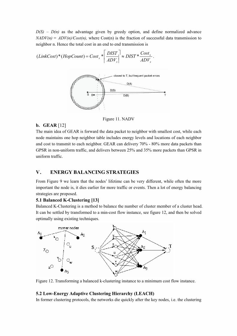
D(S) – D(n) as the advantage given by greedy option, and define normalized advance
NADV(n) = ADV(n)/Cost(n), where Cost(n) is the fraction of successful data transmission to
neighbor n. Hence the total cost in an end to end transmission is
x
x
x
xADV
CostDIST
ADV
DISTCostHopCountLinkCost **)(*)( ≈
= .
Figure 11. NADV
b. GEAR [12]
The main idea of GEAR is forward the data packet to neighbor with smallest cost, while each
node maintains one hop neighbor table includes energy levels and locations of each neighbor
and cost to transmit to each neighbor. GEAR can delivery 70% - 80% more data packets than
GPSR in non-uniform traffic, and delivers between 25% and 35% more packets than GPSR in
uniform traffic.
V.... ENERGY BALANCING STRATEGIES
From Figure 9 we learn that the nodes’ lifetime can be very different, while often the more
important the node is, it dies earlier for more traffic or events. Then a lot of energy balancing
strategies are proposed.
5.1 Balanced K-Clustering [13]
Balanced K-Clustering is a method to balance the number of cluster member of a cluster head.
It can be settled by transformed to a min-cost flow instance, see figure 12, and then be solved
optimally using existing techniques.
Figure 12. Transforming a balanced k-clustering instance to a minimum cost flow instance.
5.2 Low-Energy Adaptive Clustering Hierarchy (LEACH)
In former clustering protocols, the networks die quickly after the key nodes, i.e. the clustering
head. And the basic idea of LEACH is to using randomization to distribute the energy load
evenly hence makes every node a possibility to be key node and consume energy equally.
LEACH breaks up operation into rounds, each round consists of two phases. In Set-up phase,
an cluster-head is randomly chosen and then broadcasts “Cluster-head Advertisement” to
inform the neighbors. Then the neighbors choose the cluster head which has the best quality
of the link as its head, and send data transmission request. And the cluster head will set up
schedule for the requests. Then it’ll turn to Steady-state phase, in which data transmission is
done to cluster head, and the head transmit the data packets to the base station after signal
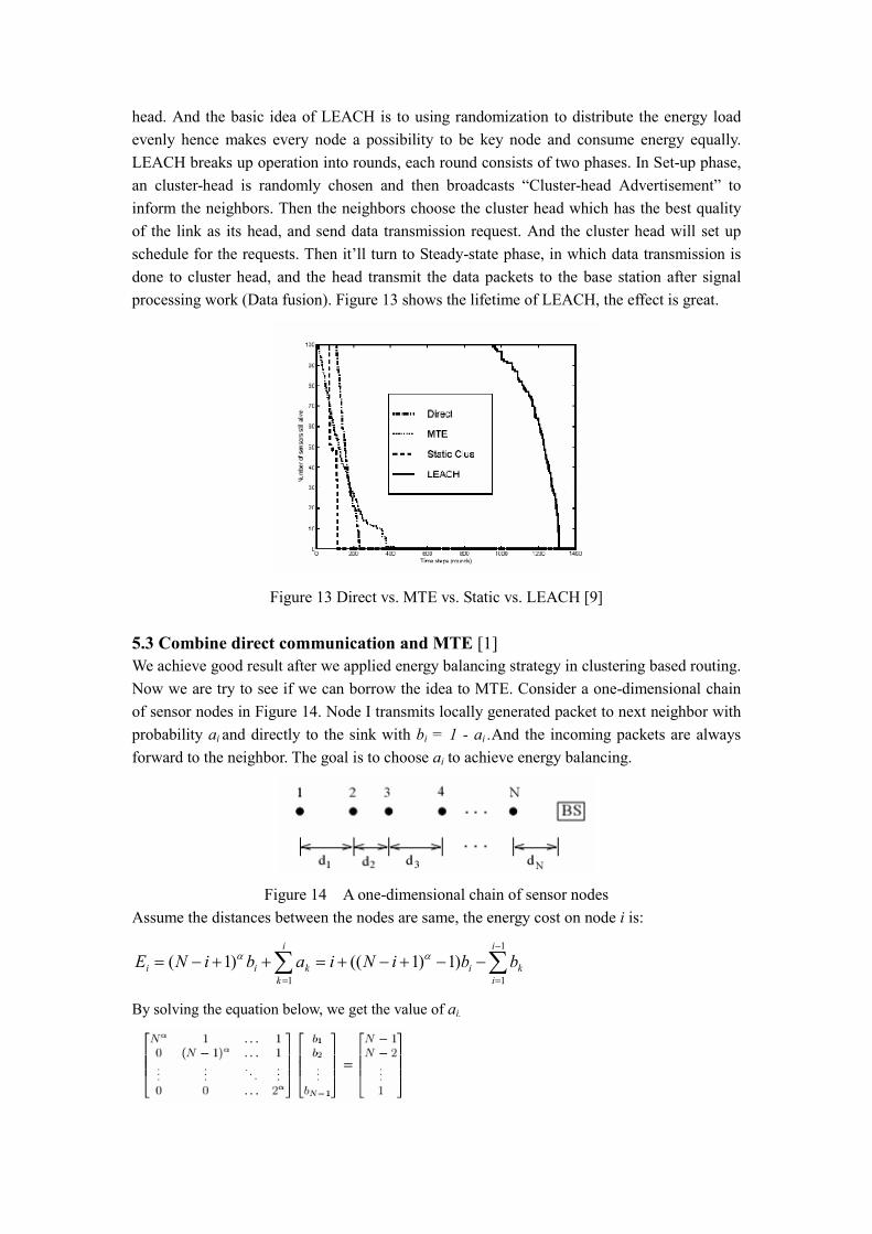
processing work (Data fusion). Figure 13 shows the lifetime of LEACH, the effect is great.
Figure 13 Direct vs. MTE vs. Static vs. LEACH [9]
5.3 Combine direct communication and MTE [1]
We achieve good result after we applied energy balancing strategy in clustering based routing.
Now we are try to see if we can borrow the idea to MTE. Consider a one-dimensional chain
of sensor nodes in Figure 14. Node I transmits locally generated packet to next neighbor with
probability ai and directly to the sink with bi = 1 - ai .And the incoming packets are always
forward to the neighbor. The goal is to choose ai to achieve energy balancing.
Figure 14 A one-dimensional chain of sensor nodes
Assume the distances between the nodes are same, the energy cost on node i is:
∑∑−
==
−−+−+=++−=1
11
)1)1(()1(i
i
ki
i
k
kii bbiNiabiNE αα
By solving the equation below, we get the value of ai.

In 10 nodes case, 14% lifetime increase with an extra energy consumption at 60% to 80%.
VI.... AN APPLICATION ORIENTED OPTIMIZATION STRATEGY
We have shown that in many cases, the lifetime of the sensor network depends on the
requirement of the application runs on it, i.e., how to optimize the lifetime of a subgraph G’(V)
in whole graph G(V). The key idea here is to release the routing load from the node outside
G’(V). For the nodes are born unequal, so we can assign a higher priority to the nodes in the
subgraph. The idea is quite general, but is very efficient. Here we introduce an application
oriented version of GPSR protocol.
We set a VIP-rate p (0 <= p <= 1) to every node, the initial value would be 0. And a
threshold h. When event arises, nodes near the spot set their priority to a higher value, say 0.8,
and it broadcast a VIP-awareness packet to its neighbor and will kept in the neighbor’s
routing table. When an intermediate node want forward a packet, it’ll follow GPSR’s
algorithm, first to see if there exists a greedy option and compares the VIP-rates, if higher
than the greedy option’s, then do greedy forwarding. Else do primeter forwarding. If no
greedy option, then follow the right hand rule. The pseudo code is list below:
a. Maintenance
All nodes maintain a single-hop neighbor table.
b. At source
Mode = greedy
c. Intermediate node
if (mode == greedy) {
greedy forwarding;
if (no_greedy_option||greedy_option_VIPrate - this.VIPrate>h)
mode = perimeter;
}
if (mode == perimeter) {
if (have left local maxima && local maxima’s VIPrate - this.VIPrate<h)
mode = greedy;
else (right-hand rule);
}
Here we provide a manual analysis of benefit along with our strategy.
Figure 15-1 is the original network, a tree based multi hop network with only one sink at the
base station. Figure 15-2 shows when an earthquake is detected, and the 2 nodes upgrade
themselves to VIPs with the rate 0.8. Figure 15-3 shows when the leaf nodes of VIPs want
transmit packets, they should find another way. Figure 15-4 indicates that nodes in other area
are detecting the earthquake event. Figure 15-5 shows the final result after optimization.
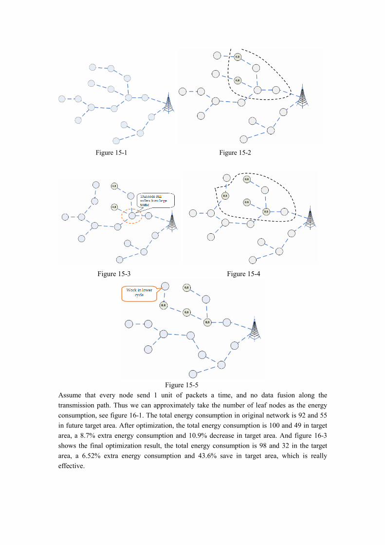
Figure 15-1 Figure 15-2
Figure 15-3 Figure 15-4
Figure 15-5
Assume that every node send 1 unit of packets a time, and no data fusion along the
transmission path. Thus we can approximately take the number of leaf nodes as the energy
consumption, see figure 16-1. The total energy consumption in original network is 92 and 55
in future target area. After optimization, the total energy consumption is 100 and 49 in target
area, a 8.7% extra energy consumption and 10.9% decrease in target area. And figure 16-3
shows the final optimization result, the total energy consumption is 98 and 32 in the target
area, a 6.52% extra energy consumption and 43.6% save in target area, which is really
effective.
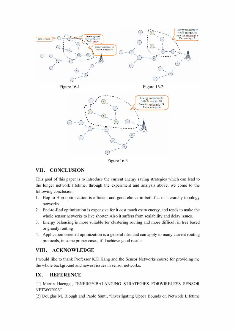
Figure 16-1 Figure 16-2
Figure 16-3
VII.... CONCLUSION
This goal of this paper is to introduce the current energy saving strategies which can lead to
the longer network lifetime, through the experiment and analysis above, we come to the
following conclusion:
1. Hop-to-Hop optimization is efficient and good choice in both flat or hierarchy topology
networks
2. End-to-End optimization is expensive for it cost much extra energy, and tends to make the
whole sensor networks to live shorter. Also it suffers from scalability and delay issues.
3. Energy balancing is more suitable for clustering routing and more difficult in tree based
or greedy routing
4. Application oriented optimization is a general idea and can apply to many current routing
protocols, in some proper cases, it’ll achieve good results.
VIII.... ACKNOWLEDGE
I would like to thank Professor K.D.Kang and the Sensor Networks course for providing me
the whole background and newest issues in sensor networks.
IX.... REFERENCE
[1] Martin Haenggi, “ENERGY-BALANCING STRATEGIES FORWIRELESS SENSOR
NETWORKS”
[2] Douglas M. Blough and Paolo Santi, “Investigating Upper Bounds on Network Lifetime

Extension for Cell-Based Energy Conservation Techniques in Stationary Ad Hoc Networks”,
MOBICOM’02
[3] J. Chang and L. Tassiulas, “Energy conserving routing in wireless ad hoc networks.”, In
Proc. IEEE INFOCOM 2000, pages 22–31, 2000.
[4] T. Brown, H. Gabow, and Q. Zhang. “Maximum flow-life curve for a wireless ad hoc
network. ”, In Proc. ACM MobiHoc 01, pages 128–136, 2001.
[5] H. Zhang, and Jennifer Hou, “On deriving the upper bound of q-lifetime for large sensor
netowrks” MobiHoc 04.
[6] E.J. Duarte-Melo and M. Liu, “Analysis of energy consumption and lifetime of
heterogeneous wireless sensor networks”, IEEE Globecom 2002
[7] F. Ye, G. Zhong, S. Lu, and L. Zhang,” Energy efficient robust sensing coverage in large
sensor networks” TR, UCLA, 2002
[8] Ritesh Madan and Sanjay Lall, “Distributed Algorithms for Maximum Lifetime Routing in
Wireless Sensor Networks”, Globecom 2004
[9] Juhana Yrjola, “Energy-Efficient Communication Protocol for Wireless Microsensor
Networks”, T-79.194 Seminar on theoretical computer science 2005
[10] Dongkyun Kim, J.J. Garcia-Luna-Aceves, “Performance analysis of power-aware route
selection protocols in mobile ad hoc networks”
[11] Seungjoon Lee and Bobby Bhattacharjee and Suman Banerjee, “Efficient Geographic
Routing in Multihop Wireless Networks”, MobiHoc 2005
[12] Yan Yu, Ramesh Govindan and Deborah Estrin “Geographical and Energy Aware Routing: a
recursive data dissemination protocol for wireless sensor networks”
[13] Soheil Ghiaki, Ankur Srivastava, Xiaojian Yang, and Majid Sarrafzadeh, “Optimal Energy Aware
Clustering in Sensor Networks”