A Survey in Mathematics for Industry Mathematics of ...math.arizona.edu/~leonk/papers/ejm.pdf · Mathematics of thermoacoustic tomography 193 Transducer MW pulse Figure 1. The TAT

Euro. Jnl of Applied Mathematics (2008), vol. 19, pp. 191–224. c© 2008 Cambridge University Press

doi:10.1017/S0956792508007353 Printed in the United Kingdom191

A Survey in Mathematics for IndustryMathematics of thermoacoustic tomography

PETER KUCHMENT1 and LEONID KUNYANSKY2

1Mathematics Department, Texas A&M University, College Station, TX 77843-3368, USA

email: [email protected] Department, University of Arizona, Tucson, AZ 77843-3368, USA

email: [email protected]

(Received 10 April 2007; revised 12 February 2008)

The article presents a survey of mathematical problems, techniques and challenges arising in

thermoacoustic tomography and its sibling photoacoustic tomography.

1 Introduction

Computerized tomography has had a huge impact on medical diagnostics. Numerous

methods of tomographic medical imaging have been developed and are being developed

(e.g., the ‘standard’ X-ray, single-photon emission, positron emission, ultrasound, magnetic

resonance, electrical impedance, optical) [62, 67, 84–86]. The designers of these modalities

strive to increase the image resolution and contrast, and at the same time to reduce the

costs and negative health effects of these techniques. However, these goals are usually

rather contradictory. For instance, some cheap and safe methods with good contrast

(like optical or electrical impedance tomography) suffer from low resolution, while some

high-resolution methods (such as ultrasound imaging) often do not provide good contrast.

Recently researchers have been developing novel hybrid methods that combine different

physical types of signals, in the hope of alleviating the deficiencies of each of the

types, while taking advantage of their strengths. The most successful example of such

a combination is the thermoacoustic tomography (TAT)1 [69, 70, 95]. Albeit not yet a

common feature in clinics, TAT scanners are actively researched, developed and already

manufactured, for instance by OptoSonics, Inc. (http://www.optosonics.com/), founded

by the pioneer of TAT, R. Kruger.

After a substantial effort, major breakthroughs have been achieved in the last few years

in the mathematical modeling of TAT. The aim of this article is to survey this recent

progress and to describe the relevant models, mathematical problems and reconstruction

procedures arising in TAT and to provide references to numerous research publications

on this topic.

1TAT is also sometimes abbreviated as TCT, which stands for thermoacoustic computed tomo-

graphy. If instead of radio-frequency waves, laser beams are used to trigger the thermoacoustic

signal, the procedure is called photoacoustic (PAT) or optoacoustic (OAT) tomography.

192 P. Kuchment and L. Kunyansky

The main thrust of this text is towards mathematical methods; considerations of

the text length, as well as authors’ background, do not let us discuss in any detail

industrial and physical set-ups and parameters of the TAT technique and limitations

of the corresponding mathematical models. Fortunately, the excellent recent surveys by

M. Xu and L.-H. V. Wang [131] and by A. A. Oraevsky and A. A. Karabutov [96, 97]

accomplish all of these tasks, and thus the reader is advised to consult with them for

all such issues (see also the recent textbook [126]). On the other hand, in spite of the

significant recent progress in mathematics of TAT, there is no comprehensive survey text

addressing in detail the relevant mathematical issues2, although the surveys [97, 131] do

mention some mathematical reconstruction techniques.

The structure of the article is as follows: Section 2 contains a brief description of the

TAT procedure. Section 3 provides the mathematical formulation of the TAT problem. In

general, it is formulated as an inverse problem for the wave equation. However, in the

case of the constant sound speed, it can also be described in terms of a spherical mean

operator (a spherical analogue of the Radon transform). The section also contains a list of

natural questions to be addressed concerning this model. These issues are then addressed

one by one in the following sections. In particular, Section 4 discusses uniqueness of

reconstruction, i.e., the question of whether the data collected in TAT is sufficient for

recovery of the information of interest. Although, for all practical purposes this issue is

resolved in Corollary 2, we provide an additional discussion of unresolved uniqueness

problems, which are probably of more academic interest. Section 5 addresses inversion

formulas and algorithms. In Section 6 the effects of having only partial data are discussed.

Section 7 contains results concerning the so-called range conditions, i.e., the conditions

that all ideal data must satisfy. Section 8 provides additional remarks and discussions of

the issues raised in the previous sections, and is followed by a bibliography. Concerning

the latter, we mention that the engineering and biomedical literature on TAT is rather

vast and no attempt has been made in this text to create a comprehensive bibliography

of the topic from the engineering prospective. The references in [95, 96, 97, 121, 124, 131]

to a large extent fill this gap. We have, however, tried to present a sufficiently complete

review of the existing literature on mathematics of TAT.

2 Thermoacoustic tomography

In TAT, a short-duration electromagnetic (EM) pulse is sent through a biological object

(e.g., a woman’s breast in mammography) with the aim of triggering a thermoacoustic

response in the tissue. As explained in [131], the radiofrequency (RF) and the visible

light frequency ranges are currently considered to be the most suitable for this purpose.

Since mathematics works exactly the same way in both of these frequency ranges, we

will not make such a distinction and will discuss just ‘an EM pulse’. For example, in

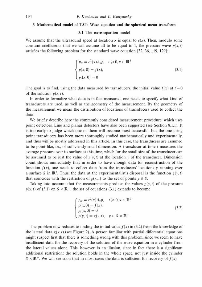
Figure 1 a microwave pulse is assumed. In most cases the pulse is spatially wide, so

that the whole object is more or less uniformly irradiated. Some part of EM energy is

2Since the submission of this article, two surveys on various topics of mathematics of TAT

[41, 105] and a special issue [64] have appeared. Two other surveys [5, 40], also of a more restricted

nature, are forthcoming in [125].

Mathematics of thermoacoustic tomography 193

Transducer

MW pulse

Figure 1. The TAT procedure.

absorbed throughout the object. The amount of energy absorbed at a location strongly

depends on the local biological properties of the cells. Oxygen saturation, concentration

of haemoglobin, density of the microvascular network (angiogenesis), ionic conductivity

and water content are among the parameters that influence the absorption strongly [131].

Thus, if the energy absorption distribution function f(x) were known, it would provide

a great diagnostic tool. For instance, it could be useful for detecting cancerous cells that

absorb several times more energy in the RF range than healthy ones [70, 97, 129, 131].

However, as an imaging tool neither RF waves nor visual light alone would provide

acceptable resolution. In the RF case, this is due to the long wavelength. One can use

shorter microwaves, but this will be at the expense of the penetration depth. In the optical

region, the problem is with the multiple scattering of light. So, a different mechanism, the

so-called photoacoustic effect [53, 119, 126, 131], is used to image f(x). Namely, the EM

energy absorption results in thermoelastic expansion and thus in a pressure wave p(x, t)

(an ultrasound signal) that can be measured by transducers placed around the object. Now

one can attempt to recover the function f(x) (the image) from the measured data p(x, t).

Such a measuring scheme, utilizing two types of waves, brings about the high resolution of

the ultrasound diagnostics and the high contrast of EM waves. It overcomes the adverse

effect of the low contrast of ultrasound with respect to soft tissue. In fact, such a low

contrast is a good thing here, allowing one to assume in the first approximation that the

sound speed is constant. This often used approximation is not always appropriate, but it

is the most studied case at the moment. Later on in this text we will describe some initial

considerations of the variable sound speed case, following [4, 46, 49, 65].

For this TAT method (and in particular, for the mathematical model described in the

next section) to work, several conditions must be met. For instance, the time duration

of the EM pulse must be shorter than the time it takes the sound wave to traverse the

smallest feature that needs to be reconstructed. The ultrasound detector must be able to

resolve the time scale of the duration of the EM pulse. On the other hand, the transducer

must be also able to detect much lower frequencies. Thus, one needs to have extra-wide-

band transducers, and these are currently available. One can find the technical discussion

of all these issues, for instance, in [97, 125, 126, 131]. In this text we will assume that all

these conditions are met and thus the mathematical models described are applicable.

In the next section we present a mathematical description of the relation between f(x)

and p(x, t) (similar mathematical problems arise in sonar [81] and radar [90] imaging, as

well as in geophysics [31]).


3 Mathematical model of TAT: Wave equation and the spherical mean transform

3.1 The wave equation model

We assume that the ultrasound speed at location x is equal to c(x). Then, modulo some

constant coefficients that we will assume all to be equal to 1, the pressure wave p(x, t)

satisfies the following problem for the standard wave equation [32, 36, 119, 129]:

⎧⎪⎪⎨⎪⎪⎩ptt = c2(x)∆xp, t 0, x ∈ 3

p(x, 0) = f(x),

pt(x, 0) = 0

(3.1)

The goal is to find, using the data measured by transducers, the initial value f(x) at t= 0

of the solution p(x, t).

In order to formalize what data is in fact measured, one needs to specify what kind of

transducers are used, as well as the geometry of the measurement. By the geometry of

the measurement we mean the distribution of locations of transducers used to collect the

data.

We briefly describe here the commonly considered measurement procedure, which uses

point detectors. Line and planar detectors have also been suggested (see Section 8.1.1). It

is too early to judge which one of them will become most successful, but the one using

point transducers has been more thoroughly studied mathematically and experimentally,

and thus will be mostly addressed in this article. In this case, the transducers are assumed

to be point-like, i.e., of sufficiently small dimension. A transducer at time t measures the

average pressure over its surface at this time, which for the small size of the transducer can

be assumed to be just the value of p(y, t) at the location y of the transducer. Dimension

count shows immediately that in order to have enough data for reconstruction of the

function f(x), one needs to collect data from the transducers’ locations y running over

a surface S in 3. Thus, the data at the experimentalist’s disposal is the function g(y, t)

that coincides with the restriction of p(x, t) to the set of points y ∈ S .

Taking into account that the measurements produce the values g(y, t) of the pressure

p(x, t) of (3.1) on S × +, the set of equations (3.1) extends to become

⎧⎪⎪⎨⎪⎪⎩ptt = c2(x)∆xp, t 0, x ∈ 3

p(x, 0) = f(x),

pt(x, 0) = 0

p(y, t) = g(y, t), y ∈ S × +

(3.2)

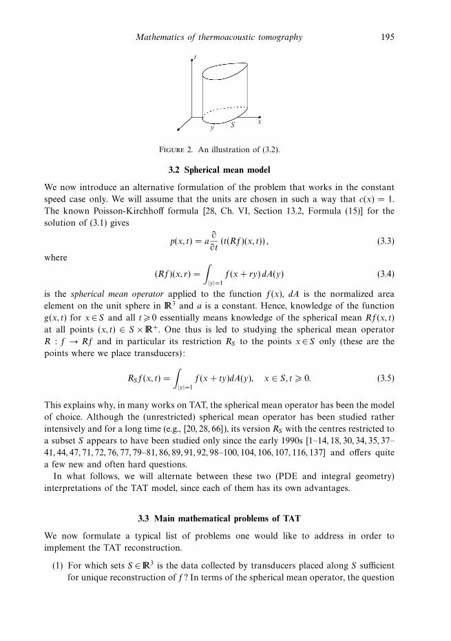
The problem now reduces to finding the initial value f(x) in (3.2) from the knowledge of

the lateral data g(x, t) (see Figure 2). A person familiar with partial differential equations

might suspect first that there is something wrong with this problem, since we seem to have

insufficient data for the recovery of the solution of the wave equation in a cylinder from

the lateral values alone. This, however, is an illusion, since in fact there is a significant

additional restriction: the solution holds in the whole space, not just inside the cylinder

S × +. We will see soon that in most cases the data is sufficient for recovery of f(x).


t

y S x

Figure 2. An illustration of (3.2).

3.2 Spherical mean model

We now introduce an alternative formulation of the problem that works in the constant

speed case only. We will assume that the units are chosen in such a way that c(x) = 1.

The known Poisson-Kirchhoff formula [28, Ch. VI, Section 13.2, Formula (15)] for the

solution of (3.1) gives

p(x, t) = a∂

∂t(t(Rf)(x, t)) , (3.3)

where

(Rf)(x, r) =

∫|y|=1

f(x+ ry) dA(y) (3.4)

is the spherical mean operator applied to the function f(x), dA is the normalized area

element on the unit sphere in 3 and a is a constant. Hence, knowledge of the function

g(x, t) for x∈ S and all t 0 essentially means knowledge of the spherical mean Rf(x, t)

at all points (x, t) ∈ S × +. One thus is led to studying the spherical mean operator

R : f → Rf and in particular its restriction RS to the points x∈ S only (these are the

points where we place transducers):

RSf(x, t) =

∫|y|=1

f(x+ ty)dA(y), x ∈ S, t 0. (3.5)

This explains why, in many works on TAT, the spherical mean operator has been the model

of choice. Although the (unrestricted) spherical mean operator has been studied rather

intensively and for a long time (e.g., [20, 28, 66]), its version RS with the centres restricted to

a subset S appears to have been studied only since the early 1990s [1–14, 18, 30, 34, 35, 37–

41, 44, 47, 71, 72, 76, 77, 79–81, 86, 89, 91, 92, 98–100, 104, 106, 107, 116, 137] and offers quite

a few new and often hard questions.

In what follows, we will alternate between these two (PDE and integral geometry)

interpretations of the TAT model, since each of them has its own advantages.

3.3 Main mathematical problems of TAT

We now formulate a typical list of problems one would like to address in order to

implement the TAT reconstruction.

(1) For which sets S ∈ 3 is the data collected by transducers placed along S sufficient

for unique reconstruction of f? In terms of the spherical mean operator, the question


is whether RS has zero kernel on an appropriate class of functions, say continuous

with compact support.

(2) If the data collected from S is sufficient, what are the relevant inversion formulas

and algorithms?

(3) How stable is the inversion?

(4) What happens if the data is ‘incomplete’?

(5) What is the space of all possible ‘ideal’ data g(t, y) collected on a surface S?

Mathematically (and in the constant sound speed case) this is the question of

describing the range of the operator RS in appropriate function spaces. This question

might seem to be unusual (for instance, to people used to partial differential

equations), but in tomography the importance of knowing the range of Radon type

transforms is well known. Such information is used to improve inversion algorithms,

complete incomplete data, discover and compensate for certain data errors, etc. (e.g.,

[34, 43–45, 60–62, 85, 86, 99, 135]).

4 Uniqueness of reconstruction

Many of the problems of interest to TAT can be formulated in any dimension d, although

the practical dimensions are only d = 3 and d = 2. We will consider an arbitrary dimension

d whenever appropriate.

Let S ⊂ d be the set of locations of the transducers and f be a compactly supported

function (one can show that for purposes of uniqueness of reconstruction problem, one

can always assume that f is smooth [7]). Does the absence of the signal on the transducers,

i.e., g(t, y) = 0 for all t and y in S , imply that f= 0? If the answer is a ‘yes,’ we call S

a uniqueness set, otherwise a non-uniqueness set. In other words, in terms of TAT, the

uniqueness sets are those for which distributing transducers along them provides enough

data for unique reconstruction of the function f(x).

In terms of the wave equation, uniqueness sets are the sets of complete observability,

i.e., such that observing the motion on this set only, one gets enough information to

reconstruct the whole oscillation. In terms of the spherical mean operator, the question is

whether the equality RSf = 0 implies that f = 0.

We will address this problem for the constant sound speed case first.

4.1 Constant speed case

As it has been discussed, the dimension count makes it clear that S must be (d − 1)-

dimensional, i.e., a surface in 3D or a curve in 2D. We will also see that most of

such surfaces are ‘good’, i.e., are uniqueness ones (or, in other words, provide enough

information for reconstruction). Thus, we should rather discuss the problem of describing

the ‘bad’, non-uniqueness sets. The following simple statement is very important and not

immediately obvious.

Lemma 1 [7, 79, 80, 137] Any non-uniqueness set S is a set of zeros of a (non-trivial)

harmonic polynomial. In particular,


(1) If there is no non-zero polynomial vanishing on S , then S is a uniqueness set.

(2) If there is no non-zero harmonic function vanishing on S , then S is a uniqueness set.

The proof of this lemma is very simple. It works under the assumption of exponential

decay of the function f(x), not necessarily of compactness of its support. It also introduces

some polynomials that play a significant role in the whole analysis of the spherical mean

operator RS .

Let k 0 be an integer. Consider the convolution

Qk(x) = |x|2k ∗ f(x) =

∫|x− y|2kf(y) dy. (4.1)

This is clearly a polynomial of degree at most 2k. Rewriting the integral in polar

coordinates centered at x and using radiality of |x− y|, one sees that Qk(x) is determined

if we know the values Rf(x, t) of the spherical mean of f centered at x:

Qk(x) = cd

∫ ∞

0

t2k+d−1Rf(x, t) dt.

In particular, if RSf ≡ 0, then each polynomial Qk vanishes on S .

Another observation that is easy to justify is that if the function f is exponentially

decaying (e.g., is compactly supported), then if all polynomials Qk vanish identically, the

function itself must be equal to zero. (This is not necessarily true any more if f and its

derivatives decay only faster than any power, rather than exponentially.)

Thus, we conclude that if f is not identically equal to zero, then there is at least one

non-zero polynomial Qk . Since, as we discussed, equality RSf = 0 implies that Qk|S = 0,

we conclude that S must be algebraic.

Now notice the following easy to verify equality (with a non-zero constant ck):

∆Qk = ckQk−1, (4.2)

where ∆ is the Laplace operator. This implies that the lowest k non-zero polynomial Qkis harmonic. Since Qk|S = 0, this proves the lemma.

Consider now the case when S is a closed (hyper-)surface (i.e., the boundary of a

bounded domain). Since, as it is well known, there is no non-zero harmonic function in

the domain that vanishes at the boundary (the spectrum of the Dirichlet Laplace operator

is strictly positive), we conclude that such S is a uniqueness set for harmonic polynomials.

Thus, we get the following important result.

Corollary 2 [7, 71] Any closed surface is a uniqueness set for the spherical mean Radon

transform.

An older alternative proof [71] of this corollary provides an additional insight into the

problem. We thus sketch it here. Let us assume for simplicity that the dimension d 3

is odd (even dimensions require a little bit more work). Suppose that the closed surface

S remains stationary (nodal) for the oscillation described by (3.1). Since the oscillation

is unconstrained and the initial perturbation is compactly supported, after a finite time,


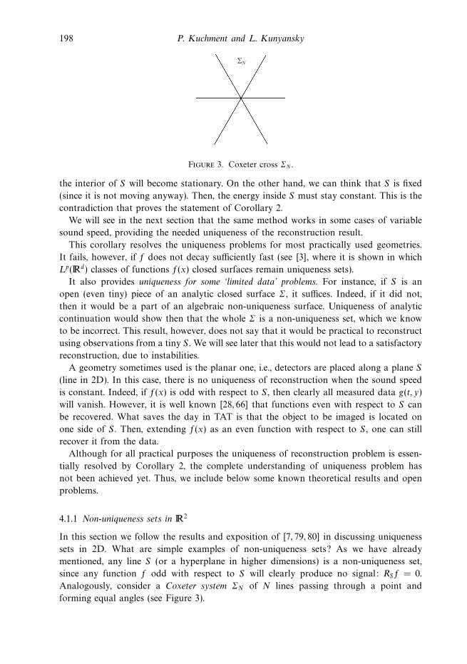
Figure 3. Coxeter cross ΣN .

the interior of S will become stationary. On the other hand, we can think that S is fixed

(since it is not moving anyway). Then, the energy inside S must stay constant. This is the

contradiction that proves the statement of Corollary 2.

We will see in the next section that the same method works in some cases of variable

sound speed, providing the needed uniqueness of the reconstruction result.

This corollary resolves the uniqueness problems for most practically used geometries.

It fails, however, if f does not decay sufficiently fast (see [3], where it is shown in which

Lp(d) classes of functions f(x) closed surfaces remain uniqueness sets).

It also provides uniqueness for some ‘limited data’ problems. For instance, if S is an

open (even tiny) piece of an analytic closed surface Σ, it suffices. Indeed, if it did not,

then it would be a part of an algebraic non-uniqueness surface. Uniqueness of analytic

continuation would show then that the whole Σ is a non-uniqueness set, which we know

to be incorrect. This result, however, does not say that it would be practical to reconstruct

using observations from a tiny S . We will see later that this would not lead to a satisfactory

reconstruction, due to instabilities.

A geometry sometimes used is the planar one, i.e., detectors are placed along a plane S

(line in 2D). In this case, there is no uniqueness of reconstruction when the sound speed

is constant. Indeed, if f(x) is odd with respect to S , then clearly all measured data g(t, y)

will vanish. However, it is well known [28, 66] that functions even with respect to S can

be recovered. What saves the day in TAT is that the object to be imaged is located on

one side of S . Then, extending f(x) as an even function with respect to S , one can still

recover it from the data.

Although for all practical purposes the uniqueness of reconstruction problem is essen-

tially resolved by Corollary 2, the complete understanding of uniqueness problem has

not been achieved yet. Thus, we include below some known theoretical results and open

problems.

4.1.1 Non-uniqueness sets in 2

In this section we follow the results and exposition of [7, 79, 80] in discussing uniqueness

sets in 2D. What are simple examples of non-uniqueness sets? As we have already

mentioned, any line S (or a hyperplane in higher dimensions) is a non-uniqueness set,

since any function f odd with respect to S will clearly produce no signal: RSf = 0.

Analogously, consider a Coxeter system ΣN of N lines passing through a point and

forming equal angles (see Figure 3).


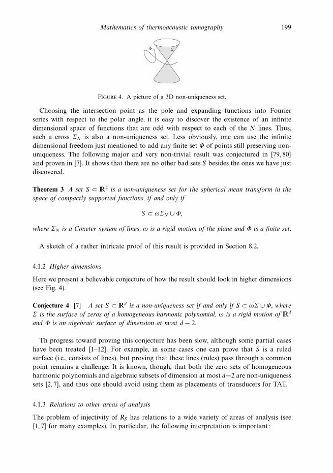
Figure 4. A picture of a 3D non-uniqueness set.

Choosing the intersection point as the pole and expanding functions into Fourier

series with respect to the polar angle, it is easy to discover the existence of an infinite

dimensional space of functions that are odd with respect to each of the N lines. Thus,

such a cross ΣN is also a non-uniqueness set. Less obviously, one can use the infinite

dimensional freedom just mentioned to add any finite set Φ of points still preserving non-

uniqueness. The following major and very non-trivial result was conjectured in [79, 80]

and proven in [7]. It shows that there are no other bad sets S besides the ones we have just

discovered.

Theorem 3 A set S ⊂ 2 is a non-uniqueness set for the spherical mean transform in the

space of compactly supported functions, if and only if

S ⊂ ωΣN ∪ Φ,

where ΣN is a Coxeter system of lines, ω is a rigid motion of the plane and Φ is a finite set.

A sketch of a rather intricate proof of this result is provided in Section 8.2.

4.1.2 Higher dimensions

Here we present a believable conjecture of how the result should look in higher dimensions

(see Fig. 4).

Conjecture 4 [7] A set S ⊂ d is a non-uniqueness set if and only if S ⊂ ωΣ ∪Φ, where

Σ is the surface of zeros of a homogeneous harmonic polynomial, ω is a rigid motion of d

and Φ is an algebraic surface of dimension at most d− 2.

Th progress toward proving this conjecture has been slow, although some partial cases

have been treated [1–12]. For example, in some cases one can prove that S is a ruled

surface (i.e., consists of lines), but proving that these lines (rules) pass through a common

point remains a challenge. It is known, though, that both the zero sets of homogeneous

harmonic polynomials and algebraic subsets of dimension at most d−2 are non-uniqueness

sets [2, 7], and thus one should avoid using them as placements of transducers for TAT.

4.1.3 Relations to other areas of analysis

The problem of injectivity of RS has relations to a wide variety of areas of analysis (see

[1, 7] for many examples). In particular, the following interpretation is important:


Theorem 5 [7, 71] The following statements are equivalent:

(1) S ⊂ d is a non-uniqueness set for the spherical mean operator.

(2) S is a nodal set for the wave equation, i.e., there exists a non-zero compactly supported

f such that the solution of the wave propagation problem

⎧⎪⎪⎪⎨⎪⎪⎪⎩∂2u

∂t2= ∆u,

u(x, 0) = 0,

ut(x, 0) = f(x)

vanishes on S for any moment of time.

(3) S is a nodal set for the heat equation, i.e., there exists a non-zero compactly supported

f such that the solution of the problem

⎧⎨⎩∂u

∂t= ∆u,

u(x, 0) = f(x)

vanishes on S for any moment of time.

The interpretation in terms of the wave equation provides important PDE tools and

insights, which have led to a recent progress [12, 38] (although it has not led yet to a

complete alternative proof of Theorem 3). The rough idea, originally introduced in [38], is

that if S is a nodal set, then it might be considered as the fixed boundary. In this case, the

signals must go around S . However, in fact, there is no obstacle, so signals can propagate

along straight lines. Thus, in order to avoid discrepancies in arrival times, S must be very

special. One can find details in [12] and in [38].

4.2 Uniqueness in the case of a variable sound speed

It is shown in [40, Theorem 4] that uniqueness of reconstruction also holds in the case of a

smoothly varying (strictly positive) sound speed, if the source function f(x) is completely

surrounded by the observation surface S (in other words, if there is no ultrasound signal

coming from outside of S). The proof uses the celebrated unique continuation result by

D. Tataru [120].

One can also establish uniqueness of reconstruction in the case where the source is not

necessarily completely surrounded by S . However, here we need to impose an additional

non-trapping condition on the sound speed. We assume that the sound speed is strictly

positive, c(x) > c > 0, and such that c(x) − 1 has compact support, i.e., c(x) = 1 for a

large x.


Consider the Hamiltonian system in 2nx,ξ with the Hamiltonian H = c2(x)

2|ξ|2:⎧⎪⎪⎪⎪⎪⎨⎪⎪⎪⎪⎪⎩

x′t =

∂H

∂ξ= c2(x)ξ

ξ′t = −∂H

∂x= −1

2∇

(c2(x)

)|ξ|2

x|t=0 = x0, ξ|t=0 = ξ0.

(4.3)

The solutions of this system are called bicharacteristics and their projections into nx are

rays.

We will assume that the following non-trapping condition holds: all rays (with ξ0 0)

tend to infinity when t → ∞.

Theorem 6 [4] Under the non-trapping conditions formulated above, compactly suppor-

ted function f(x) is uniquely determined by the data g measured on S for all times. (No

assumption of f being supported inside S is imposed.)

One should mention that ray trapping can occur for some sound speed profiles. For

instance, if c(x) = |x| for some range r1 < |x| < r2, then there are rays trapped in

this spherical shell. We are not sure what happens in this case to the uniqueness of

reconstruction statement of Theorem 6 and inversion formula of Theorem 7.

5 Reconstruction: Formulas and examples

Here we will address the procedures of actual reconstruction of the source f(x) from the

data g(t, y) measured by transducers.

5.1 Constant sound speed

We assume here that the sound speed is constant and normalized to be equal to 1.

5.1.1 Inversion formulas

Before we move to our case of interest (which is spheres centered on a closed surface S

surrounding the object to be imaged), we briefly refer to related but somewhat different

work. Namely, the problem of recovering functions from integrals over spheres centered

on a (hyper)plane S has attracted a lot of attention over the years. Although, as mentioned

before, there is no uniqueness in this case (functions odd with respect to S are annihilated),

even functions can be recovered. Thus also functions supported on one side of the plane

can be as well, by means of their even extension. Many explicit inversion formulas and

procedures have been obtained for this situation [18, 30, 35, 44, 47, 68, 86, 89, 98, 99, 111,

112, 115]. In particular, Fourier transform methods are useful here. We will not provide

any details here, since this acquisition geometry does not seem very useful. In particular,

this is due to ‘invisibility’ of some parts of the interfaces (see Section 6) which arises

from truncating the plane. The same problem is encountered with some other unbounded

acquisition surfaces, such as a surface of an ‘infinitely’ long cylinder.


Thus, it is more practical to place transducers along a closed surface surrounding the

object. The simplest surface of this type is a sphere.

5.1.2 Fourier expansion methods

Let us assume that S is the unit sphere in n. We would like to reconstruct a function f(x)

supported inside S from the known values of its spherical integrals g(y, r) with centres on

S:

g(y, r) =

∫n−1

f(y + rω)rn−1 dω, y ∈ S.

The first inversion procedures for the case of spherical acquisition were described in [91]

in 2D and in [92] in 3D. These solutions were obtained by harmonic decomposition of the

measured data and the sought function, and by equating coefficients of the corresponding

Fourier series (a la A. Cormack’s method for the X-ray CT).

In particular, the 2D algorithm of [91] is based on the Fourier decomposition of f and

g in angular variables:

f(x) =

∞∑−∞

fk(ρ)eikϕ, x = (ρ cos(ϕ), ρ sin(ϕ)) (5.1)

g(y(θ), r) =

∞∑−∞

gm(r)eikθ, y = (R cos(θ), R sin(θ)).

Following [91] we consider the Hankel transform gm,J(λ) of the Fourier coefficients gm(r)

(divided by 2πr)

gm,J(λ) =

∫ 2R

0

gm(r)J0(λr) dr = H0

(gm(r)

2πr

). (5.2)

To simplify the presentation we introduce the convolution GJ(λ, y) of the sought function

with the Bessel function J0(λ|x− y|),

GJ(λ, y) =

∫Ω

f(x)J0(λ|x− y|) dx. (5.3)

One can notice that gm,J(λ) are the Fourier coefficients of GJ(λ, y) in θ:

gm,J(λ) =1

2π

∫ 2π

0

GJ(λ, y)e−imθ dθ. (5.4)

Now the coefficients fm(ρ) can be recovered from gm(r) by application of the addition

theorem for the Bessel function J0(λ|x− y|):

J0(λ|x− y|) =

∞∑−∞

Jm(λ|x|)Jm(λ|y|)e−im(ϕ−θ). (5.5)

Indeed, by substituting equations (5.1) and (5.5) into (5.3), and (5.3) into (5.4) one obtains

gm,J(λ) = 2πJm(λ|R|)∫ 2R

0

fm(ρ)Jm(λρ)ρ dρ = Hm(fm(ρ)),


where Hm is the m-th order Hankel transform. Since the latter transform is self-invertible,

the coefficients fm(ρ) can be recovered by the following formula:

fm(ρ) = Hm

[gm,J(λ)

Jm(λ|R|)

]= Hm

(1

Jm(λ|R|)H0

[gm(r)

2πr

]), (5.6)

which is the main result of [91]. The function f(x) can now be reconstructed by summing

series (5.1).

Note that the above method requires a division of the Hankel transform of the measured

data by Bessel functions Jm that have infinitely many zeros. Theoretically, there is no

problem; the Hankel transform H0[gm(r)2πr

] has to have zeros that would cancel those in

the denominator. However, since the measured data always contain some error, the exact

cancellation is not likely to happen, and one needs a sophisticated regularization scheme

to keep the total error bounded.

This problem can be avoided by replacing in (5.2) the Bessel function J0 by the Hankel

function H (1)0 :

gm,H (λ) =

∫ 2R

0

gm(r)H (1)0 (λr) dr.

The addition theorem for H (1)0 (λ|x− y|) takes the form

H(1)0 (λ|x− y|) =

∞∑−∞

Jm(λ|x|)H (1)m (λ|y|)e−im(ϕ−θ),

and by proceeding as before one can obtain the following formula for fm(ρ):

fm(ρ) = Hm

[gm,H (λ)

H(1)m (λ|R|)

]= Hm

(1

H(1)m (λ|R|)

∫ 2R

0

gm(r)H (1)0 (λr) dr

).

Unlike Jm, Hankel functions H (1)m (t) do not have zeros for any real values of t and therefore

problems with division by zeros do not arise in this amended version of the method [91].

This derivation can be repeated in 3D, with the exponentials eikθ replaced by the

spherical harmonics, and with cylindrical Bessel functions replaced by their spherical

counterparts. By doing this one will arrive at the Fourier series method of [92]. Our use

of Hankel function H (1)0 above is similar to the way the authors of [92] utilized spherical

Hankel function h(1)0 to avoid the divisions by zero.

5.1.3 Filtered backprojection methods

The most popular way of inverting Radon transform for tomography purposes is by using

filtered backprojection-type formulas, which involve filtration in Fourier domain followed

(or preceded) by a backprojection. In the case of the set of spheres centred on a closed

surface (e.g., a sphere) S , one expects such a formula to involve a filtration with respect

to the radius variable and then some integration over the set of spheres passing through

the point of interest. For quite a while, no such formula had been discovered, and even its

existence had been questioned. This did not prevent practitioners from the reconstructions,

since good approximate inversion formulas (parametrices) could be developed, followed


by an iterative improvement of the reconstruction (see, e.g. the reconstruction procedures

in [128, 129, 132–134], and especially [106, 107]).

The first set of exact inversion formulas of filtered backprojection type was discovered

in [38]. These formulas were obtained only in odd dimensions. Several different variations

of such formulas (different in terms of the exact order of the filtration and backprojection

steps) were developed. Let us denote by g(p, r) = r2RSf the spherical integral, rather than

the average, of f. Then various versions of the 3D inversion formulas that reconstruct a

function f(x) supported inside S from its spherical mean data RSf read

f(x) = − 1

8π2R∆x

∫∂B

g(y, |y − x|) dA(y),

f(x) = − 1

8π2R

∫∂B

(d2

dt2g(y, t)

) ∣∣∣t=|y−x|

dA(y), (5.7)

f(x) = − 1

8π2R

∫∂B

(d

dt

(1

t

d

dt

g(y, t)

t

)) ∣∣∣t=|y−x|

dA(y).

Recently, analogous formulas were obtained for even dimensions in [37]. Denoting by g,

as before the spherical integrals (rather than averages) of f, the formulas of [37] in 2D

look as follows:

f(x) =1

2πR∆

∫∂B

∫ 2R

0

g(y, t) log(t2 − |x− y|2) dt dl(y), (5.8)

or

f(x) =1

2πR

∫∂B

∫ 2R

0

∂

∂t

(t

∂

∂t

g(y, t)

t

)log(t2 − |x− y|2) dt dl(y), (5.9)

A different set of explicit inversion formulas that work in arbitrary dimensions was

presented in [77]:

f(x) =1

4(2π)n−1div

∫∂B

n(y)h(y, |x− y|) dA(y). (5.10)

Here

h(y, t) =

∫+

[Y (λt)

( ∫ 2R

0

J(λt′)g(y, t′) dt′)

− J(λt)

( ∫ 2R

0

Y (λt′)g(y, t′) dt′)]λ2n−3 dλ, (5.11)

J(t) =Jn/2−1(t)

tn/2−1, Y (t) =

Yn/2−1(t)

tn/2−1,

Jn/2−1(t) and Yn/2−1(t) are respectively the Bessel and Neumann functions of order n/2−1,

and n(y) is the vector of exterior normal to ∂B.

In 2D equations (5.10), (5.11) can be simplified to yield the following reconstruction

formula:

f(x) = − 1

2π2div

∫∂B

n(y)

[∫ 2R

0

g(y, t′)1

|x− y|2 − t′2dt′

]dl(y).


A similar simplification is also possible in 3D resulting in the formula

f(x) =1

8π2div

∫∂B

n(y)

(1

t

d

dt

g(y, t)

t

) ∣∣∣∣∣∣∣t=|y−x|

dA(y). (5.12)

Equation (5.12) is equivalent to one of the formulas derived in [130] for the 3D case. It is

interesting to notice that the ‘universal’ formula of [130] holds for all geometries when the

backprojection-type formulas are known: spherical, cylindrical and planar. It is not very

likely that such explicit formulas would be available for any closed surfaces S different

from spheres (see a related discussion in [15, 31]).

5.1.4 Series solutions for arbitrary geometries

Although, as we have just mentioned, we do not expect such explicit formulas to be

derived for non-spherical closed surfaces S , there is, however, a different approach [78]

that theoretically works for any closed S and that is practically useful in some non-

spherical geometries.

Let λ2m and um(x) be the eigenvalues and normalized eigenfunctions of the Dirichlet

Laplacian −∆ on the interior Ω of a closed surface S:

∆um(x) + λ2mum(x) = 0, x ∈ Ω, Ω ⊆ n, (5.13)

um(x) = 0, x ∈ S,

||um||22 ≡∫Ω

|um(x)|2 dx = 1.

As before, we would like to reconstruct a compactly supported function f(x) from the

known values of its spherical integrals g(y, r) with centres on S:

g(y, r) =

∫ωn−1

f(y + rω)rn−1 dω, y ∈ S.

We notice that um(x) is the solution of the Dirichlet problem for the Helmholtz equation

with zero boundary conditions and the wave number λm, and thus it admits the Helmholtz

representation

um(x) =

∫∂Ω

Φλm (|x− y|) ∂

∂num(y) ds(y), x ∈ Ω, (5.14)

where Φλm (|x−y|) is a free-space rotationally invariant Green’s function of the Helmholtz

equation (5.13).

The eigenfunctions um(x)∞0 form an orthonormal basis in L2(Ω). Therefore, f(x) can

be represented by the series

f(x) =

∞∑m=0

αmum(x) (5.15)

with

αm =

∫Ω

um(x)f(x) dx.


Since f(x) ∈ C10 , series (5.15) converges pointwise. A reconstruction formula of αm, and

thus of f(x), will result if we substitute representation (5.14) into (5.15) and interchange

the order of integration. Indeed, after a brief calculation we will get

αm =

∫Ω

um(x)f(x) dx =

∫∂Ω

I(y, λm)∂

∂num(y) dA(x), (5.16)

where

I(y, λ) =

∫Ω

Φλ(|x− y|)f(x) dx. (5.17)

Certainly, the need to know the spectrum and eigenfunctions of the Dirichlet Laplacian

imposes a severe constraint on the surface S . However, there are simple cases when the

eigenfunctions are well known, and fast summation formulas for the corresponding series

are available. Such is the case of a cubic measuring surface S (see [78]); the eigenfunctions

um are products of sine functions:

um(x) =8

R3sin

πm1x1

Rsin

πm2x2

Rsin

πm3x3

R, (5.18)

where m = (m1, m2, m3), m1, m2, m3 ∈ , and the eigenvalues are easily found as well:

λm = π2|m|2/R2. (5.19)

Sum (5.15) is just a regular 3D Fourier sine series easily computable by application

of the Fast Fourier Sine transform algorithm. The algorithmic trick that allows one

to calculate the coefficients αm quickly consists in first computing integrals (5.17) on

a uniform mesh in λ. This is easily done by a 1D Fast Fourier Cosine transform

algorithm, with Φλ(t) = cos(λt)/t. The normal derivatives of um(x) are also products of

sine functions, this time 2D ones. This, in turn, permits rapid evaluation of the integrals∫∂ΩiI(y, λ) ∂

∂num(y) dA(x) for each mesh value of λ, and for each one of the six faces

∂Ωi, i = 1, . . . , 6, of the cube. Finally, the computation of αm using equation (5.16) reduces

to the interpolation in the spectral parameter λ, since the integrals in the right-hand side

of this equation have been computed for the mesh values of this parameter (not for

λm). Due to the oscillatory nature of the integrals (5.17) a low-order interpolation here

would lead to inaccurate reconstructions. Luckily, however, these integrals are analytic

functions of the parameter λ (due to the finite support of g). Hence, high-order polynomial

interpolation is applicable, and numerics yields very good results.

The algorithm we just described requires O(m3 logm) floating point operations if the

reconstruction is to be performed on an m × m × m Cartesian grid, from comparably

discretized data measured on a cubic surface. In practical terms, it yields reconstructions in

the matter of several seconds on grids with total number of nods exceeding a million [78].

5.1.5 Time reversal (backpropagation) methods

In the constant speed case, the following approach is possible in 3D [38]: due to the

validity of the Huygens’ principle (i.e., the signal escapes from any bounded domain in

finite time), the pressure p(t, x) inside S will become equal to zero for any time T larger


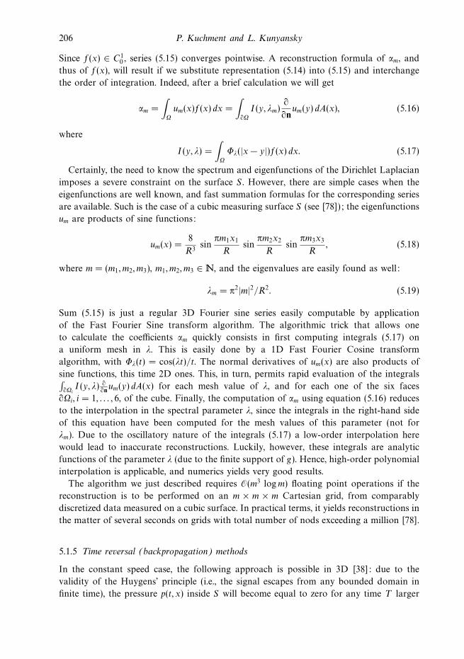
Figure 5. A mathematical phantom in 3D (left) and its reconstruction using an analytic inversion

formula.

than the time required to cross the domain (i.e., time that it takes the sound to move

along the diameter of S , which for c = 1 equals the diameter). Thus, one can impose zero

conditions on p(t, x) for t = T and solve the wave equation (3.2) back in time, using the

measured data g as the boundary values. The solution of this well-posed problem at t = 0

gives the desired source function f(x). Such methods have been successfully implemented

[25].

Although in 2D or in presence of sound speed variations Huygens’ principle does not

hold any more, and thus the signal theoretically will stay forever, one can find good

approximate solutions using a similar approach [4, 46, 49]; see discussions of the variable

speed case later.

5.1.6 Examples of reconstructions and additional remarks about the inversion formulas

It is worth noting that although formulas (5.7)–(5.8) and (5.10)–(5.12) will yield identical

results when applied to functions that can be represented as the spherical mean Radon

transform of a function supported inside S , they are in general not equivalent when

applied to functions with larger supports. Simple examples (e.g., of f being the char-

acteristic set of a large ball containing S) show that these two types of formulas

provide different reconstructions. They also are not equivalent on data that contain

errors.

It is well known that different analytic inversion formulas in tomography can behave

differently in numerical implementation (e.g., in terms of their stability). However, nu-

merical implementation seems to show that the analytic (backprojection type) formulas

(5.7)–(5.12), in spite of them being not equivalent on data that involve errors, work equally

well. See, for example, the results of an analytic formula reconstruction in 3D shown in

Figure 5.

An interesting observation is that backprojection formulas (5.7)–(5.12) do not recon-

struct the function f correctly inside the surface S , if f has support reaching outside S .

For instance, applying the reconstruction formulas to the function RS (χ|x|3) leads to an

incorrect reconstruction of the value of f = χ|x|3 inside S = |x| 1. (Here by χV we

denote the characteristic function of the set V , i.e., it takes the value 1 in V and zero


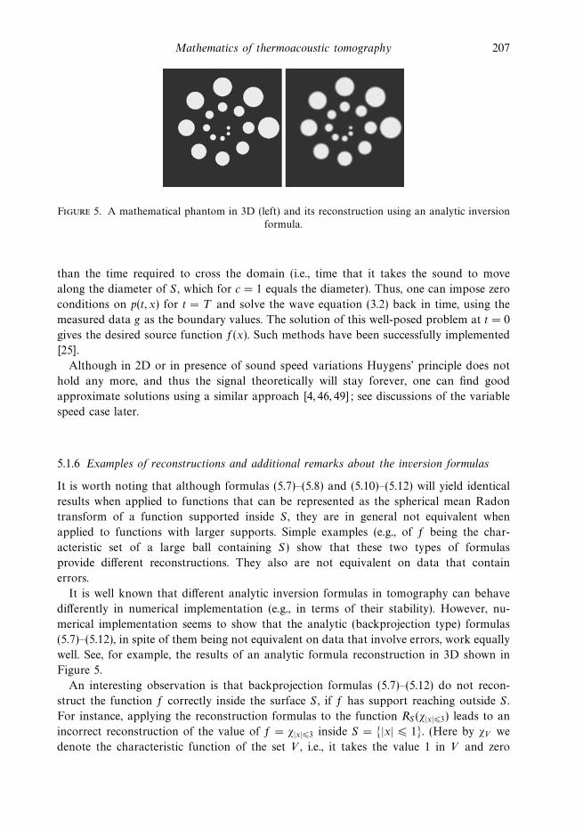
Figure 6. A perturbed reconstruction due to presence of two additional balls outside S (not

shown in the picture).

Figure 7. In the phantom shown on the left, most disks are located outside the square acquisition

surface S indicated by the dotted line. This does not perturb the reconstruction inside S (right).

outside. So, χ|x|3 is the characteristic function of the ball of radius 3 centered at the

origin.)

As another example, if one adds to the phantom shown in Figure 5 two balls to the

right of the surrounding sphere S , this leads to strong artifacts, as seen in Figure 6.

What is the reason for such a distortion? If one does not know in advance that f has

support inside S , the backprojection formulas shown before use insufficient information

to recover a function with a larger support, and thus uniqueness of reconstruction is lost.

Then the formulas misinterpret the data, wrongly assuming that they came from a function

supported inside S and thus reconstructing the function incorrectly. The backprojection

formulas make significant use of the assumption of f being supported inside S and also

of the time derivative of the pressure vanishing at time t = 0. It is not clear whether such

formulas are possible without these assumptions.

Notice that the series reconstruction of the preceding section is free of such problem.

For example, the reconstruction shown in Figure 7 confirms this.

The reason of such robustness of the series reconstructions is that the only assumption

they use is a sufficiently fast decay of the solution (pressure) inside S . This condition

holds, for instance, when f has a compact support (not necessarily surrounded by the

observation surface S) and when the sound speed satisfies a non-trapping condition (see

the next section), e.g., is constant. See [46] for this discussion.


5.2 Reconstruction in the variable speed case

We will assume here that the sound speed c(x) is smooth, positive, constant for a large x

and non-trapping. Although most analytic techniques we described above do not work in

the variable speed case, some formulas can be derived and algorithms can be designed.

This work is at an early stage and the results described hereafter most surely can and will

be improved.

5.2.1 ‘Analytic’ inversions

Let us denote by Ω the interior of the observation surface S , i.e., the area where the object

to be imaged is located. Consider in Ω the operator A = −c2(x)∆ with zero Dirichlet

conditions on the boundary S = ∂Ω. This operator is self-adjoint, if considered in the

weighted space L2(Ω; c−2(x)).

We also denote by E the operator of harmonic extension, which transforms a function

φ on S to a harmonic function on Ω which coincides with φ on S .

The following result provides a formula for reconstructing f from the data g:

Theorem 7 [4] The function f(x) in (3.2) can be reconstructed in Ω as follows:

f(x) = (Eg|t=0) −∫ ∞

0

A− 12 sin (τA

12 )E(gtt)(x, τ) dτ. (5.20)

The validity of this result hinges upon decay estimates for the solution (so-called local

energy decay [33, 122, 123]), which hold under the non-trapping condition. These estimates

guarantee a qualified decay of the solution p(t, x) inside any bounded region, e.g., in Ω,

when time t increases. In odd dimensions decay is exponential, but only polynomial in

even dimensions. The decay can be used instead of Huygens’ principle to solve the wave

equation backwards, starting at infinite time. This leads to the formula (5.20).

Due to functions of the operator A being involved, it is not that clear how explicit and

practical this formula can be made. For instance, it would be interesting to see whether

one can derive from (5.20) a backprojection inversion formula for the case of a constant

sound speed and S being a sphere (we have already seen that such formulas are known).

5.2.2 Backpropagation

The decay at large values of time can be used as follows: for a sufficiently large T , one

can assume that the solution is practically zero at t = T . Thus, imposing zero initial

conditions at t = T and solving in the reverse time direction, one arrives at t = 0 to an

approximation of f(x). Numerical experiments [46, 49] show that this works even under

worst of circumstances, in 2D and with a trapping sound speed.

5.2.3 Eigenfunction expansions

One natural way to try to use the formula (5.20) is to use the eigenfunction expansion of

the operator A in Ω (assuming that such expansion is known). This immediately leads to

the following result:


Theorem 8 Under the same conditions on the sound speed as before, function f(x) can be

reconstructed inside Ω from the data g in (3.2), as the following L2(B)-convergent series:

f(x) =∑k

fkψk(x), (5.21)

where the Fourier coefficients fk can be recovered using one of the following formulas:

fk = λ−2k gk(0) − λ−3

k

∫ ∞

0

sin (λkt)g′′k (t) dt,

fk = λ−2k gk(0) + λ−2

k

∫ ∞

0

cos (λkt)g′k(t) dt, or (5.22)

fk = −λ−1k

∫ ∞

0

sin (λkt)gk(t) dt = −λ−1k

∫ ∞

0

∫S

sin (λkt)g(x, t)∂ψk∂ν

(x) dx dt,

and

gk(t) =

∫S

g(x, t)∂ψk∂ν

(x) dx.

Here ν denotes the external normal to S .

One notices that this is a generalization to the variable sound speed case of the

expansion method of [78], discussed in Section 5.1.4. An interesting feature is that, unlike

in [78], we do not need to know the whole space Green’s function for A (which is certainly

not known). However, it is not clear yet how feasible numerical implementation of this

approach could be.

6 Partial data: ‘Visible’ and ‘invisible’ singularities

Uniqueness of reconstruction does not imply practical recoverability, since the reconstruc-

tion procedure might be severely unstable. This is well known to be the case, for instance,

in incomplete data situations in X-ray tomography, and even for complete data problems

in some imaging modalities, such as the electrical impedance tomography [72, 76, 85, 86].

In order to describe the results below, we need to explain the notion of the wave front

set WF(f) of a function f(x). This set carries detailed information on singularities of

f(x). It consists of pairs (x, ξ) of a point x in space and a wave vector (Fourier domain

variable) ξ 0. It is easier to say what it means that a point (x0, ξ0) is not in the wave

front set WF(f). This means that one can smoothly cut off f to zero at a small distance

from x0 in such a way that the Fourier transform φf(ξ) of the resulting function φ(x)f(x)

decays faster than any power of ξ in directions that are close to the direction of ξ0. We

remind the reader that if this Fourier transform decays that way in all directions, then

f(x) is smooth near the point x0. So, the wave front set consists of pairs (x0, ξ0) such

that f is not smooth near x0, and ξo indicates why it is not: the Fourier transform does

not decay well in this direction. For instance, if f(x) consists of two smooth pieces joined

non-smoothly across a smooth interface Σ, then WF(f) contains pairs (x, ξ) such that x

is in Σ and ξ is normal to Σ at x. One can find simple introduction to the notions of

microlocal analysis, such as the wave front set, for instance in [118].


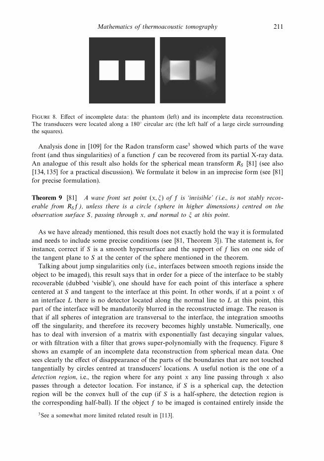
Figure 8. Effect of incomplete data: the phantom (left) and its incomplete data reconstruction.

The transducers were located along a 180 circular arc (the left half of a large circle surrounding

the squares).

Analysis done in [109] for the Radon transform case3 showed which parts of the wave

front (and thus singularities) of a function f can be recovered from its partial X-ray data.

An analogue of this result also holds for the spherical mean transform RS [81] (see also

[134, 135] for a practical discussion). We formulate it below in an imprecise form (see [81]

for precise formulation).

Theorem 9 [81] A wave front set point (x, ξ) of f is ‘invisible’ (i.e., is not stably recov-

erable from RSf), unless there is a circle (sphere in higher dimensions) centred on the

observation surface S , passing through x, and normal to ξ at this point.

As we have already mentioned, this result does not exactly hold the way it is formulated

and needs to include some precise conditions (see [81, Theorem 3]). The statement is, for

instance, correct if S is a smooth hypersurface and the support of f lies on one side of

the tangent plane to S at the center of the sphere mentioned in the theorem.

Talking about jump singularities only (i.e., interfaces between smooth regions inside the

object to be imaged), this result says that in order for a piece of the interface to be stably

recoverable (dubbed ‘visible’), one should have for each point of this interface a sphere

centered at S and tangent to the interface at this point. In other words, if at a point x of

an interface L there is no detector located along the normal line to L at this point, this

part of the interface will be mandatorily blurred in the reconstructed image. The reason is

that if all spheres of integration are transversal to the interface, the integration smooths

off the singularity, and therefore its recovery becomes highly unstable. Numerically, one

has to deal with inversion of a matrix with exponentially fast decaying singular values,

or with filtration with a filter that grows super-polynomially with the frequency. Figure 8

shows an example of an incomplete data reconstruction from spherical mean data. One

sees clearly the effect of disappearance of the parts of the boundaries that are not touched

tangentially by circles centred at transducers’ locations. A useful notion is the one of a

detection region, i.e., the region where for any point x any line passing through x also

passes through a detector location. For instance, if S is a spherical cap, the detection

region will be the convex hull of the cup (if S is a half-sphere, the detection region is

the corresponding half-ball). If the object f to be imaged is contained entirely inside the

3See a somewhat more limited related result in [113].


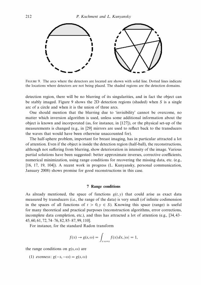
Figure 9. The arcs where the detectors are located are shown with solid line. Dotted lines indicate

the locations where detectors are not being placed. The shaded regions are the detection domains.

detection region, there will be no blurring of its singularities, and in fact the object can

be stably imaged. Figure 9 shows the 2D detection regions (shaded) when S is a single

arc of a circle and when it is the union of three arcs.

One should mention that the blurring due to ‘invisibility’ cannot be overcome, no

matter which inversion algorithm is used, unless some additional information about the

object is known and incorporated (as, for instance, in [127]), or the physical set-up of the

measurements is changed (e.g., in [29] mirrors are used to reflect back to the transducers

the waves that would have been otherwise unaccounted for).

The half-sphere problem, important for breast imaging, has in particular attracted a lot

of attention. Even if the object is inside the detection region (half-ball), the reconstructions,

although not suffering from blurring, show deterioration in intensity of the image. Various

partial solutions have been suggested: better approximate inverses, corrective coefficients,

numerical minimization, using range conditions for recovering the missing data, etc. (e.g.,

[16, 17, 19, 104]). A recent work in progress (L. Kunyansky, personal communication,

January 2008) shows promise for good reconstructions in this case.

7 Range conditions

As already mentioned, the space of functions g(t, y) that could arise as exact data

measured by transducers (i.e., the range of the data) is very small (of infinite codimension

in the spaces of all functions of t > 0, y ∈ S). Knowing this space (range) is useful

for many theoretical and practical purposes (reconstruction algorithms, error corrections,

incomplete data completion, etc.), and thus has attracted a lot of attention (e.g., [34, 43–

45, 60, 61, 72, 74–76, 82, 85–87, 99, 110].

For instance, for the standard Radon transform

f(x) → g(s, ω) =

∫x·ω=s

f(x) dx, |ω| = 1,

the range conditions on g(s, ω) are

(1) evenness: g(−s,−ω) = g(s, ω)


Figure 10. An illustration to Theorem 10.

(2) moment conditions: for any integer k 0, the kth moment

Gk(ω) =

∫ ∞

−∞skg(ω, s) ds

extends from the unit circle of vectors ω to a homogeneous polynomial of degree k

in ω.

The evenness condition is obviously necessary and is kind of ‘trivial’. It seems that the only

non-trivial conditions are the moment ones. However, here the standard Radon transform

misleads us, as it often happens. In fact, for more general transforms of Radon type it

is often easy (or easier) to find analogues of the moment conditions, while analogues of

the evenness conditions are often elusive (see [72, 74, 75, 85, 86, 93] devoted to the case of

SPECT (single-photon emission tomography)). The same happens in TAT.

Let us deal first with the case of a constant sound speed, when one can think of the

spherical mean transform RS instead of the wave equation model. An analogue of the

moment conditions was already present implicitly (without saying that these were range

conditions) in [7, 79, 80] and explicitly formulated as such in [104]. Indeed, our discussion

in Section 4 of the polynomials Qk provides the following conditions of moment type:

Moment conditions [7, 79, 80, 104] on data g(p, r) = RSf(p, r) look as follows: for any

integer k 0, the moment

Mk(ω) =

∫ ∞

0

r2k+d−1g(p, r) dr

can be extended from S to a (non-homogeneous) polynomial Qk(x) of degree at most 2k.

These conditions, however, are incomplete, and in fact infinitely many others, which

play the role of an analogue of evenness, need to be added.

Complete range descriptions for RS when S is a circle in 2D were discovered in [13] and

then in odd dimensions in [39]. They were then extended to any dimension and interpreted

in several different ways in [6]. These conditions happen to be intimately related to PDEs

and spectral theory.

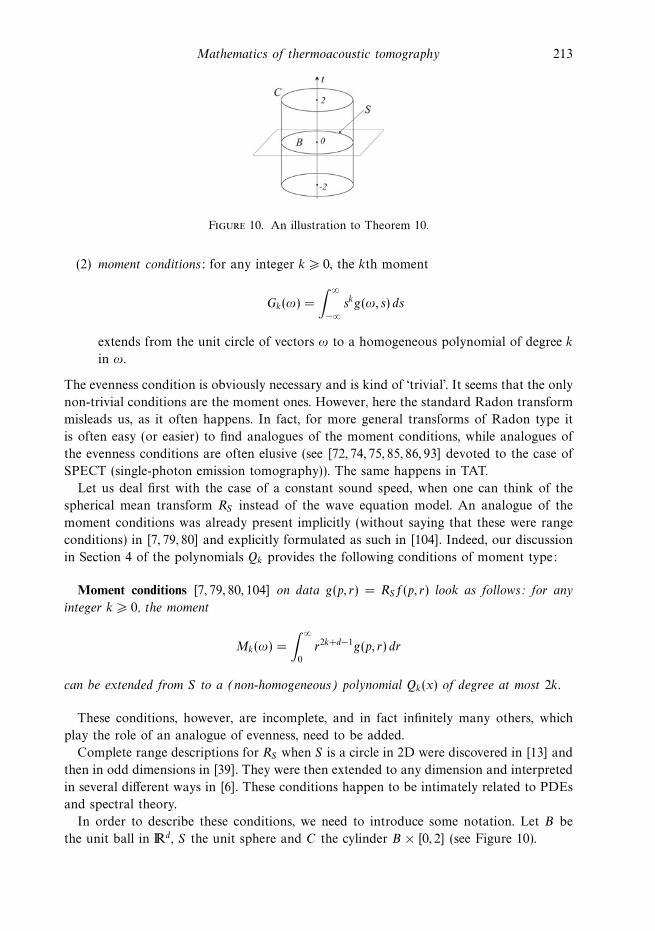
In order to describe these conditions, we need to introduce some notation. Let B be

the unit ball in d, S the unit sphere and C the cylinder B × [0, 2] (see Figure 10).


We introduce the spherical mean operator RS as before:

RSf(x, t) =

∫|y|=1

f(x+ ty) dA(y), x ∈ S.

Several different range descriptions for RS were provided in [6], out of which we only

show a few.

Theorem 10 [6] The following three statements are equivalent:

(1) The function g ∈ C∞0 (S × [0, 2]) is representable as RSf for some f ∈ C∞

0 (B). (In

other words, g represents an ideal (free of errors) set of TAT data.)

(2) (a) The moment conditions are satisfied.

(b) Let −λ2 be any eigenvalue of the Laplace operator in B with zero Dirichlet

conditions and ψλ be the corresponding eigenfunction. Then the following ortho-

gonality condition is satisfied:∫S×[0,2]

g(x, t)∂νψλ(x)jn/2−1(λt)tn−1 dx dt = 0. (7.1)

Here jp(z) = cpJp(z)

zpis the so-called spherical Bessel function.

(3) (a) The moment conditions are satisfied.

(b) Let g(x, λ) =∫g(x, t)jn/2−1(λt)t

n−1 dt. Then, for any m ∈ , the m-th spherical

harmonic term gm(x, λ) of g(x, λ) vanishes at all zeros λ 0 of the Bessel

function Jm+n/2−1(λ).

Remark 11 [6]

(1) In odd dimensions, moment conditions are not necessary, and thus conditions 2(b)

or 3(b) suffice. (A similar earlier result was established for a related transform in

[39].)

(2) The range conditions (2) of the previous theorem are also necessary when S is the

boundary of any bounded domain, not necessarily a sphere.

(3) An analogue of these conditions can be derived for a variable sound speed (without

non-trapping conditions imposed).

8 Concluding remarks

8.1 Variations of the TAT procedure

8.1.1 Planar and linear transducers

Assuming that transducers are point-like is clearly an approximation, and in fact a trans-

ducer measures the average pressure over its area. It has been rightfully claimed that the

point approximation for transducers should lead to some blurring in the reconstructions.

This, as well as intricacies of reconstructions from the data obtained by point transducers,


triggered recent proposals for different types of transducers (see [23, 24, 54–59, 101, 102]).

In these papers, it was suggested to use either planar or line detectors.

In the first case [55], the detectors are assumed to be large and planar, ideally assumed

to be approximations of infinite planes that are placed tangentially to a sphere containing

the object. Thus, the data one collects is the integrals of the pressure over these planes,

for all values of t > 0. If one takes the standard 3D Radon transform of the pressure

p(x, t) with respect to x:

P (x, t) → q(s, t, ω) =

∫x·ω=s

p(x, t) dA(x),

where dA is the surface measure and ω is a unit vector in 3, this is well known to

reduce the 3D Laplace operator ∆x to the second derivative ∂2/∂s2 [34, 43–45, 60, 61], and

thus the 3D wave equation to the string vibration problem. The measured data provide

the boundary conditions for this problem. The initial conditions in (3.1) mean evenness

with respect to time, and thus the standard d’Alambert formula leads to the immediate

realization that the measured data is just the 3D Radon transform of f(x). Thus, the

reconstruction boils down to the well-known inversion formulas for the Radon transform.

Another proposal [23, 24, 54, 56, 57, 101, 102] is to use line detectors that provide line

integrals of the pressure p(x, t). Such detectors can be implemented optically, using either

Fabry-Perot [24], or Mach-Zehnder [102] interferometers.

Suppose that the object is surrounded by a surface that is rotation-invariant with

respect to the z-axis. It is suggested to place the line detectors perpendicular to the z-axis

and tangential to the surface. The same consideration as above then shows that after

the 2D Radon (or X-ray, which in 2D is the same) transform in each plane orthogonal

to z-axis, the 3D wave equation converts into the 2D one for the Radon data. The

measurements provide the boundary data. Thus, the reconstruction boils down to solving

a 2D problem similar to the one in the case of point detectors, and then inverting the 2D

Radon transform.

Due to the recent nature of these two projects, it appears to be too early to judge

which one will be superior in the end. For instance, it is not clear beforehand, whether

the approximation of infinite size (length, area) of the linear or planar detectors works

better than the zero dimension approximation for point detectors. Further developments

will resolve these questions, but probably each type of the detectors will find its niche.

8.1.2 Direct imaging techniques

Some direct imaging techniques have been suggested, which might not require mathemat-

ical reconstructions. See, for instance, [88] about an acoustic lens system.

8.1.3 Using contrast agents

Contrast agents to improve TAT imaging have been developed (e.g., [27]).


8.1.4 Passive thermoacoustic imaging

The TAT model we have considered can be called ‘active thermoacoustic tomography’,

due to the set-up when the practitioner creates the signal. There has been some recent

development of the ‘passive thermoacoustic tomography’, where the thermoacoustic signal

is used to image the temperature sources present inside the body. One can find a survey

of this area in [103].

8.2 Uniqueness

8.2.1 Sketch of the proof of Theorem 10

We provide here a brief outline of the rather technical proof of Theorem 10.

Suppose that f is compactly supported, not identically zero, and such that RSf = 0.

Our previous considerations show that one can assume that S is an algebraic curve (not

a straight line) that is contained in the set of zeros of a non-trivial harmonic polynomial.

Now one touches the boundary of the support of f from outside by a circle centered on

S . Then microlocal analysis of the operator RS (which happens to be an analytic Fourier

Integral Operator (FIO) [21, 48, 50–52, 73, 108]) shows that, due to the equality RSf = 0,

at the tangency point the vector co-normal to the sphere should not belong to the analytic

wave front of f (microlocal regularity of solutions of RSf = 0). This, for instance, can

be extracted from the results of [117]. On the other hand, a theorem by Hormander and

Kashiwara [63, Theorem 8.5.6] shows that this vector must be in the analytic wave front

set, since f = 0 on one side of the sphere (a microlocal version of uniqueness of analytic

continuation). This way, one gets a contradiction. Unfortunately, the life is not so easy,

and the proof sketched above does not go through smoothly, due to possible cancellation

of wave fronts at different tangency points. Then one has to involve the geometry of zeros

of harmonic polynomials [42] to exclude the possibility of such a cancellation.

Thus, the proof uses microlocal analysis and geometry of zeros of harmonic polynomials.

Both these tools have their limitations. For instance, the microlocal approach (at least,

in the form it is used in [7]) does not allow considerations of non-compactly supported

functions. Thus, the validity of the theorem for arbitrarily fast decaying, but not compactly

supported, functions is still not established, although it most certainly holds. On the

other hand, the geometric part does not work that well in dimensions larger than 2.

Development of new approaches is apparently needed in order to overcome these hurdles.

A much simpler PDE approach has emerged recently [38] (see also [12] and the next

section), although its achievements have been limited so far.

8.2.2 Some open problems concerning uniqueness

As already mentioned, one can consider the practical problems about uniqueness resolved.

However, the mathematical understanding of the uniqueness problem for the restricted

spherical mean operators RS is still unsatisfactory. Here are some questions that still await

their resolution:

(1) Describe uniqueness sets in dimensions larger than 2 (prove Conjecture 4). Recent

limited progress as well as variations on this theme can be found in [1–12].


(2) Prove Theorem 3 without using microlocal and harmonic polynomial tools.

(3) Prove Theorem 3 on uniqueness sets S under the condition of sufficiently fast decay

(rather than compactness of support) of the function. Very little is known for the

case of functions without compact support. The main known result is of [3], which

describes for which values of 1 p ∞ the result of Corollary 2 holds for f ∈ Lp:

Theorem 12 [3] Let S be the boundary of a bounded domain in d and f ∈ Lp(d) such

that RSf ≡ 0. If p 2d/(d − 1), then f ≡ 0 (and thus S is injectivity set for this space).

This fails for any p > 2d/(d− 1).

8.3 Inversion

Although closed form (backprojection type) inversion formulas are available now for the

cases of S being a plane (and object on one side from it), a cylinder and a sphere, there

is still some mystery surrounding this issue.

(1) Can one write a backprojection-type inversion formula in the case of the constant

sound speed for a closed surface S which is not a sphere? We suspect that the

answer to this question is negative (see also related discussion in [15, 31]).

(2) The inversion formulas for S being a sphere assume that the object to be imaged is

inside S . One can check on simplest examples that if the support of the function f(x)

reaches outside S , the inversion formulas do not reconstruct the function correctly

even inside of S . See [5, 46] for a discussion. Do backprojection-type formulas exist

that do not have this deficiency?

(3) I. Gelfand’s school of integral geometry has developed a marvellous machinery of

the so-called κ operator, which provides a general approach to inversion and range

descriptions for transforms of Radon type [43, 44]. In particular, it has been applied

to the case of integration of various collections (‘complexes’) of spheres in [44, 47].

This consideration seems to suggest that one should not expect explicit closed form

inversion formulas for RS , even when S is a sphere. We, however, know that such

formulas have been discovered [38, 77]. This apparent controversy has not been

resolved.

(4) Can one derive any more explicit analytic formulas from (5.20)?

(5) Can the series expansion formulas of Theorem 8 be efficiently implemented?

It has been suggested [15, 26] to use in the TAT problem not only the values of the

pressure measured by transducers on the observation surface S , but its normal derivative

to S as well. If one knows both, then taking Fourier transform in the time variable and

using the whole space Green’s function for the Helmholtz equation leads immediately to

a reconstruction formula for the solution (which seems to be much simpler than what is

proposed in [26]). The problem is that this normal derivative is not measured by TAT

devices. Under some circumstances (e.g., when there are no sources of ultrasound outside

S), one can prove the theoretical possibility of recovering the missing normal derivative.

In rare cases (planar, cylindrical or spherical surface S), when involvement of the normal

derivative can be eliminated (e.g., [15, 31]), this might lead to feasible inversion algorithms,


but in these cases, explicit and nicely implementable analytic inversion formulas are already

available. So, jury is still out on the issue of plausibility of this procedure.

8.4 Stability

Stability of inversion when S is a sphere surrounding the support of f(x) is the same

as for the standard Radon transform, as the results of [100] and the second statement

of Theorem 11 show. However, if the support reaches outside, although Corollary 2 still

guarantees uniqueness of reconstruction, stability (at least for the parts outside S) is gone.

Indeed, Theorem 9 shows that some parts of singularities of f outside S will not be stably

‘visible.’

8.5 Range

As Theorem 9 states, the range conditions 2 and 3 of Theorem 10 are necessary also for

non-spherical closed surfaces S and for functions with support outside S . They, however,

are not expected to be sufficient, since Theorem 9 indicates that one might expect non-

closed ranges in some cases. The same applies for non-constant sound speed case.

8.6 Sound speed recovery

A question that has started attracting attention recently is the one of simultaneous

recovery from TAT data of the sound speed c(x) and the object f. Clearly, one needs to

worry about the recovery of the speed first. Only first steps in this direction have been

taken. For instance, in [136], the problem is treated numerically with encouraging results.

However, even the question of whether the sound speed is uniquely determined by TAT

data has not been resolved. So far, it is known that if the speed is constant and f is

supported strictly inside S , the speed is uniquely determined by the measured data [46].

It seems reasonable to try to use the range conditions of Theorem 10 to recover the

sound speed. These conditions contain information of two types: the support conditions

and an infinite series of orthogonality conditions. One wonders whether the orthogonality

conditions help with the recovery of the speed. Although we do not know the complete

answer to this question, even for constant speed the situation is not trivial. One can

show that orthogonality conditions alone (without support conditions) do not uniquely

determine the constant sound speed [46]. On the other hand, there is some kind of local

uniqueness [46].

8.7 Attenuation effects

In all the models discussed so far in this article, attenuation of ultrasound has been

neglected. It seems that this important TAT feature has not yet been sufficiently studied.

See [22, 83, 114] for this issue and additional references.

Acknowledgements

The work of the first author was partially supported by the NSF DMS grants 0604778

and 0648786. The second author was partially supported by the DOE grant DE-FG02-

03ER25577 and NSF DMS grant 0312292. Part of this work was completed when the


first author was at the Isaac Newton Institute for Mathematical Sciences. The authors

express their gratitude to the NSF, DOE and INI for this support. The authors thank

M. Agranovsky for useful discussions, M. Anastasio, G. Beylkin, P. Burgholzer, D. Finch,

M. Klibanov, G. Paltauf, and P. Stefanov for providing preprints and references, and the

reviewers and editors for very helpful remarks.

References

[1] Agranovsky, M. (1997) Radon transform on polynomial level sets and related problems.

Israel Math. Conf. Proc. 11, 1–21.

[2] Agranovsky, M. (2000) On a problem of injectivity for the Radon transform on a paraboloid.

Analysis, geometry, number theory: The mathematics of Leon Ehrenpreis In: Contemp.

Math. 251, AMS, Providence, RI, pp. 1–14.

[3] Agranovsky, M., Berenstein, C. & Kuchment, P. (1996) Approximation by spherical waves

in Lp-spaces. J. Geom. Anal. 6(3), 365–383.

[4] Agranovsky, M. & Kuchment, P. (2007) Uniqueness of reconstruction and an inversion

procedure for thermoacoustic and photoacoustic tomography with variable sound speed.

Inv. Prob. 23, 2089–2102.

[5] Agranovsky, M., Kuchment, P. & Kunyansky, L. (2007) On reconstruction formulas and

algorithms for the thermoacoustic and photoacoustic tomography. To appear in [125].

[6] Agranovsky, M., Kuchment, P. & Quinto, E. T. (2007) Range descriptions for the spherical

mean Radon transform. J. Funct. Anal. 248, 344–386.

[7] Agranovsky, M. & Quinto, E. T. (1996) Injectivity sets for the Radon transform over circles

and complete systems of radial functions. J Funct. Anal. 139, 383–414.

[8] Agranovsky, M. & Quinto, E. T. (2001) Geometry of stationary sets for the wave equation

in n: The case of finitely suported initial data. Duke Math. J. 107(1), 57–84.

[9] Agranovsky, M. & Quinto, E. T. (2003) Stationary sets for the wave equation in crystallo-

graphic domains. Trans. AMS 355(6), 2439–2451.

[10] Agranovsky, M. & Quinto, E. T. (2006) Remarks on stationary sets for the wave equation.

Integral Geom. Tomography, Contemp. Math. 405, 1–11.

[11] Agranovsky, M., Volchkov, V. V. & Zalcman, L. (1999) Conical uniqueness sets for the

spherical Radon transform. Bull. London Math. Soc. 31(4), 363–372.

[12] Ambartsoumian, G. & Kuchment, P. (2005) On the injectivity of the circular Radon trans-

form. Inv. Prob. 21, 473–485.

[13] Ambartsoumian, G. & Kuchment, P. (2006) A range description for the planar circular

Radon transform. SIAM J. Math. Anal. 38(2), 681–692.

[14] Ambartsoumian, G. & Patch, S. (2007) Thermoacoustic tomography: Numerical results. In:

Alexander A. Oraevsky, Lihong V. Wang (editors) Proceedings of SPIE 6437, Photons Plus

Ultrasound: Imaging and Sensing 2007: The Eighth Conference on Biomedical Thermoacous-

tics, Optoacoustics, and Acousto-optics, p. 64371B, SPIE-International Society for Optical

Engine, Bellingham, Washington.

[15] Anastasio, M. A., Zhang, J., Modgil, D. & Riviere, P. J. (2007) Application of inverse

source concepts to photoacoustic tomography, Inv. Prob. 23, S21–S35.

[16] Anastasio, M., Zhang, J., Pan, X., Zou, Y., Ku, G. & Wang, L. V. (2005) Half-time image

reconstruction in thermoacoustic tomography. IEEE Trans. Med. Imaging 24, 199–210.

[17] Anastasio, M. A., Zhang, J., Sidky, E. Y., Yu Zou, Dan Xia & Xiaochuan. (2005). Feasibility

of half-data image reconstruction in 3D reflectivity tomography with a spherical aperture,

IEEE Trans. Med. Imaging 24(9), 1100–1112.

[18] Andersson, L.-E. (1988) On the determination of a function from spherical averages. SIAM

J. Math. Anal. 19(1), 214–232.


[19] Andreev, V. G., Popov, D. A., Sushko, D. V., Karabutov, A. A. & Oraevsky, A. A. (2002)

Image reconstruction in 3D optoacoustic tomography system with hemispherical transducer

array. In: Proc. SPIE 4618, p. 1605-7422/02.

[20] Asgeirsson, L. (1937) Uber eine Mittelwerteigenschaft von Losungen homogener linearer

partieller Differentialgleichungen zweiter Ordnung mit konstanten Koeffizienten. Ann. Math.

113, 321–346.

[21] Beylkin, G. (1984) The inversion problem and applications of the generalized Radon trans-

form. Comm. Pure Appl. Math. 37, 579–599.

[22] Burgholzer, P., Grun, H., Haltmeier, M., Nuster, R. & Paltauf, G. (2007) Compensation

of acoustic attenuation for high-resolution photoacoustic imaging with line detectors using

time reversal. In: Proceedings SPIE number 6437.75 Photonics West, BIOS 2007, San Jose,

CA.

[23] Burgholzer, P., Hofer, C., Matt, G. J., Paltauf, G., Haltmeier, M. & Scherzer, O.

(2006) Thermoacoustic tomography using a fiber-based Fabry-Perot interferometer as an

integrating line detector. In: Proc. SPIE 6086, pp. 434–442.

[24] Burgholzer, P., Hofer, C., Paltauf, G., Haltmeier, M. & Scherzer, O. (2005) Ther-

moacoustic tomography with integrating area and line detectors. IEEE Trans. Ultrasonics,

Ferroelectrics, Frequency Control 52(9), 1577–1583.

[25] Burgholzer, P., Matt, G., Haltmeier, M. & Patlauf, G. (2007) Exact and approximate

imaging methods for photoacoustic tomography using an arbitrary detection surface. Phys.

Rev. E 75, 046706.

[26] Clason, C. & Klibanov, M. (2007) The quasi-reversibility method in thermoacoustic tomo-

graphy in a heterogeneous medium. SIAM J. Sci. Comput. 30, 1–23.

[27] Copland, J. A. et al. (2004) Bioconjugated gold nanoparticles as a molecular based contrast

agent: Implications for imaging of deep tumors using optoacoustic tomography. Mol.

Imaging Biol. 6(5), 341–349.

[28] Courant, R. & Hilbert, D. (1962) Methods of Mathematical Physics, Vol. II: Partial Differ-

ential Equations, Interscience, New York.

[29] Cox, B. T., Arridge, S. R. & Beard, P. C. (2007). Photoacoustic tomography with a limited-

aperture planar sensor and a reverberant cavity. Inv. Prob. 23, S95–S112.

[30] Denisjuk, A. (1999) Integral geometry on the family of semi-spheres. Fract. Calc. Appl. Anal.

2(1), 31–46.

[31] Devaney, A. J. & Beylkin, G. (1984) Diffraction tomography using arbitrary transmitter and

receiver surfaces. Ultrasonic Imaging 6, 181–193.

[32] Diebold, G. J., Sun, T. & Khan, M. I. (1991) Photoacoustic monopole radiation in one, two,

and three dimensions. Phys. Rev. Lett. 67(24), 3384–3387.

[33] Egorov, Yu. V. & Shubin, M. A. (1992) Partial Differential Equations I. Encyclopaedia of

Mathematical Sciences, Springer-Verlag, Berlin, 30, 1–259.

[34] Ehrenpreis, L. (2003) The Universality of the Radon Transform, Oxford University Press,

Oxford.

[35] Fawcett, J. A. (1985) Inversion of n-dimensional spherical averages. SIAM J. Appl. Math.

45(2), 336–341.

[36] Finch, D. V. (2005) On a thermoacoustic transform. In: Proc. Fully 3D Reconstruction Radi-

ology Nuclear Medicine, Salt Lake City, 5–9 July 2005. Available online at http://www.ucair.

med.utah.edu/3D05/PaperPDF/3D05proceedingspart4- pages143-202.pdf

[37] Finch, D., Haltmeier, M. & Rakesh (2007) Inversion of spherical means and the wave

equation in even dimensions. SIAM J. Appl. Math. 68(2), 392–412.

[38] Finch, D., Patch, S. & Rakesh (2004) Determining a function from its mean values over a

family of spheres. SIAM J. Math. Anal. 35(5), 1213–1240.

[39] Finch, D. & Rakesh (2006) The range of the spherical mean value operator for functions

supported in a ball. Inv. Prob. 22, 923–938.

[40] Finch, D. & Rakesh (2007) Recovering a function from its spherical mean values in two and

three dimensions. To appear in [125].


[41] Finch, D. & Rakesh (2007) The spherical mean value operator with centers on a sphere. Inv.

Prob. 23(6), S37–S50.

[42] Flatto, L., Newman, D. J. & Shapiro, H. S. (1966) The level curves of harmonic functions.

Trans. Amer. Math. Soc. 123, 425–436.

[43] Gelfand, I., Gindikin, S. & Graev M. (1980) Integral geometry in affine and projective

spaces. J. Sov. Math. 18, 39–167.

[44] Gelfand, I., Gindikin, S. & Graev M. (2003) Selected Topics in Integral Geometry. Transl.

Math. Monogr. vol. 220, AMS, Providence, RI.

[45] Gelfand, I., Graev M. & Vilenknin, N. (1965) Generalized Functions, vol. 5: Integral Geo-

metry and Representation Theory, Academic Press, New York.

[46] Georgieva-Hristova, Y., Kuchment, P. & Nguyen, L. (2007) On reconstruction and time

reversal in thermoacoustic tomography, preprint.

[47] Gindikin, S. (1995) Integral geometry on real quadrics. In: Lie groups and Lie algebras: E.

B. Dynkin’s Seminar, Amer. Math. Soc. Transl. Ser. 2, 169, AMS, Providence, RI, pp. 23–31.

[48] Greenleaf, A. & Uhlmann, G. (1990) Microlocal techniques in integral geometry. Contemp.

Math. 113, 149–155.

[49] Grun, H., Haltmeier, M., Paltauf, G. & Burgholzer, P. (2007) Photoacoustic tomography

using a fiber based Fabry-Perot interferometer as an integrating line detector and image

reconstruction by model-based time reversal method. In: Proc. SPIE, 6631, p. 663107.

[50] Guillemin, V. (1975) Fourier integral operators from the Radon transform point of view.

Proc. Symposia Pure Math. 27, 297–300.

[51] Guillemin, V. (1985) On some results of Gelfand in integral geometry. Proc. Symposia Pure

Math. 43, 149–155.

[52] Guillemin, V. & Sternberg S. (1977) Geometric Asymptotics. AMS, Providence, RI.

[53] Gusev, V. E. & Karabutov, A. A. (1993) Laser Optoacoustics, American Institute of Physics,

New York.

[54] Haltmeier, M., Burgholzer, P., Hofer, C., Paltauf, G., Nuster, R. & Scherzer, O. (2005)

Thermoacoustic tomography using integrating line detectors. Ultrasonics Symp. 1, 166–

169.

[55] Haltmeier, M., Burgholzer, P., Paltauf, G. & Scherzer, O. (2004) Thermoacoustic com-

puted tomography with large planar receivers. Inv. Prob. 20, 1663–1673.

[56] Haltmeier, M. & Fidler, T. Mathematical challenges arising in thermoacoustic tomography

with line detectors, preprint arXiv:math.AP/0610155.

[57] Haltmeier, M., Paltauf, G., Burgholzer, P. & Scherzer, O. (2005) Thermoacoustic tomo-

graphy with integrating line detectors. In: Proc. SPIE 5864, p. 586402-8.

[58] Haltmeier, M., Scherzer, O., Burgholzer, P. & Paltauf, G. (2005) Thermoacous-

tic computed tomography with large planar receivers. ECMI Newslett. 37, 31–34.

http://www.it.lut.fi/mat/EcmiNL/ecmi37/

[59] Haltmeier, M., Schuster, T. & O. Scherzer (2005) Filtered backprojection for thermoacous-

tic computed tomography in spherical geometry. Math. Methods Appl. Sci. 28, 1919–1937.

[60] Helgason, S. (1980) The Radon Transform, Birkhauser, Basel.

[61] Helgason, S. (2000) Groups and Geometric Analysis, AMS, Providence, RI.

[62] Herman, G. (editor) (1979) Topics in Applied Physics, Vol. 32: Image Reconstruction from

Projections Springer-Verlag, Berlin.

[63] Hormander, L. (1983) The Analysis of Linear Partial Differential Operators, Vol. 1, Springer-

Verlag, New York.

[64] Inverse Problems (2007) (a special issue devoted to thermoacoustic tomography) 23(6).

[65] Jin, X. & Wang, L. V. (2006) Thermoacoustic tomography with correction for acoustic speed

variations. Phy. Med. Biol. 51, 6437–6448.

[66] John, F. (1971) Plane Waves and Spherical Means Applied to Partial Differential Equations,

Dover, New York.

[67] Kak, A. C. & Slaney, M. (2001) Principles of Computerized Tomographic Imaging, SIAM,

Philadelphia, PA.


[68] Kostli K. P., Frenz, M., Bebie, H. & Weber H. P. (2001) Temporal backward projection

of optoacoustic pressure transients using Fourier transform methods. Phys. Med. Biol. 46,

1863–1872

[69] Kruger, R. A., Kiser, W. L., Reinecke, D. R. & Kruger, G. A. (2003) Thermoacoustic

computed tomography using a conventional linear transducer array. Med. Phys. 30(5),

856–860.

[70] Kruger, R. A., Liu. P., Fang, Y. R. & Appledorn, C. R. (1995) Photoacoustic ultrasound

(PAUS) reconstruction tomography. Med. Phys. 22, 1605–1609.

[71] Kuchment, P. (1993), unpublished.

[72] Kuchment, P. (2006) Generalized transforms of radon type and their applications. In:

American Mathematical Society Short Course, 3–4 January 2005, Atlanta, GA, Proc. Symp.

Appl. Math. vol. 63, AMS, Providence RI, pp. 67–91.

[73] Kuchment, P., Lancaster, K. & Mogilevskaya, L. (1995) On local tomography. Inv. Prob.

11, 571–589.

[74] Kuchment, P. & Lvin S. (1990) Paley-Wiener theorem for the exponential Radon transform.

Acta Applicandae Mathematicae (18), 251–260.

[75] Kuchment, P. & Lvin S. (1991) The range of the exponential radon transform. Sov. Math.

Dokl. 42(1), 183–184.

[76] Kuchment, P. & Quinto, E. T. (2003). Some problems of integral geometry arising in

tomography. In: The University of the Radon Transform, Oxform University Press, Oxford,

Capter XI.

[77] Kunyansky, L. (2007) Explicit inversion formulae for the spherical mean Radon transform.

Inv. Prob. 23, 737–783.

[78] Kunyansky, L. (2007) A series solution and a fast algorithm for the inversion of the spherical

mean Radon transform. Inv. Prob. 23, S11–S20.

[79] Lin, V. & Pinkus, A. (1993) Fundamentality of ridge functions. J. Approx. Theory 75, 295–311.

[80] Lin, V. & Pinkus, A (1994) Approximation of multivariate functions. In H. P. Dikshit &

C. A. Micchelli (editors), Advances in Computational Mathematics, World Scientific, pp. 1–9.

[81] Louis, A. K. & Quinto, E. T. (2000) Local tomographic methods in Sonar. In Surveys on

Solution Methods for Inverse Problems, Springer, Vienna, David Colton, Heinz W. Engl,

Alfred K. Louis, and Joyce R. McLaughlin, pp. 147–154.

[82] Lvin S. (1994) Data correction and restoration in emission tomography. In E. T. Quinto, M.

Cheney & P. Kuchment (editors), Tomography, Impedance Imaging, and Integral Geometry,

Lectures in Appl. Math., Vol. 30, AMS, Providence, RI, pp. 149–155.

[83] Maslov, K., Zhang, H. F. & Wang, L. V. (2007) Effects of wavelength-dependent fluence

attenuation on the noninvasive photoacoustic imaging of hemoglobin oxygen saturation in

subcutaneous vasculature in vivo. Inv. Prob. 23, S113–S122.

[84] Mathematics and Physics of Emerging Biomedical Imaging, The National Academies Press,

1996. Available online at http://www.nap.edu/catalog.php?record id=5066#toc.

[85] Natterer, F. (1986) The Mathematics of Computerized Tomography, Wiley, New York.

[86] Natterer, F. & Wubbeling, F. (2001) Mathematical Methods in Image Reconstruction, Mono-

graphs on Mathematical Modeling and Computation 5, SIAM, Philadelphia, PA.

[87] Nessibi, M. M., Rachdi, L. T. & Trimeche, K. (1995) Ranges and inversion formulas for

spherical mean operator and its dual. J. Math. Anal. Appl. 196(3), 861–884.

[88] Niederhauser, J. J., Jaeger, M., Lemor, R., Weber, P. & Frenz, M. (2005) Combined

ultrasound and optoacoustic system for real-time high-contrast vascular imaging in vivo.

IEEE Trans. Med. Imaging 24, 436–440.

[89] Nilsson, S. (1997) Application of Fast Backprojection Techniques for Some Inverse Problems

of Integral Geometry. Linkoeping studies in science and technology, Dissertation 499,

Department of Mathematics, Linkoeping University, Linkoeping, Sweden.

[90] Nolan, C. J. & Cheney, M. (2002) Synthetic aperture inversion. Inv. Prob. 18, 221–235.

[91] Norton, S. J. (1980) Reconstruction of a two-dimensional reflecting medium over a circular

domain: Exact solution. J. Acoust. Soc. Am. 67, 1266–1273.


[92] Norton, S. J. & Linzer, M. (1981) Ultrasonic reflectivity imaging in three dimensions: Exact

inverse scattering solutions for plane, cylindrical, and spherical apertures. IEEE Trans.

Biomed. Eng., 28, 200–202.

[93] Novikov, R. (2002) On the range characterization for the two-dimensional attenuated X-ray

transform. Inv. Prob. 18, 677–700.

[94] Olafsson, G. & Quinto, E. T. (editors), (2006) The Radon transform, inverse problems, and

tomography. In: American Mathematical Society Short Course 3–4 January 2005, Atlanta,

GA, Proc. Symp. Appl. Math. vol. 63, AMS, Providence, RI.

[95] Oraevsky, A. A., Esenaliev, R. O., Jacques, S. L. Tittel, F. K. (1996) Laser optoacoustic

tomography for medical diagnostics principles. In: Proc. SPIE 2676, p. 22.

[96] Oraevsky, A. A. & Karabutov, A. A. (2002) Time-Resolved Detection of Optoacous-

tic Profiles for Measurement of Optical Energy Distribution in Tissues. In: V. V.

Tuchin (editors), Handbook of Optical Biomedical Diagonstics, SPIE, Bellingham, WA,

Chapter 10.

[97] Oraevsky A. A. & Karabutov, A. A. (2003) Optoacoustic tomography. In: T. Vo-Dinh

(editors), Biomedical Photonics Handbook, CRC Press, Boca Raton, FL, Chapter 34, 34-1–

34-34.

[98] Palamodov, V. P. (2000) Reconstruction from limited data of arc means. J. Fourier Anal.

Appl. 6(1), 25–42.

[99] Palamodov, V. P. (2004) Reconstructive Integral Geometry, Birkhauser, Basel.

[100] Palamodov, V. (2007) Remarks on the general Funk-Radon transform and thermoacoustic

tomography. Preprint arxiv: math.AP/0701204.

[101] Paltauf, G., Burgholzer, P., Haltmeier, M. & Scherzer, O. (2005) Thermoacoustic tomo-

graphy using optical line detection. In: Proc. SPIE 5864, pp. 7–14.

[102] Paltauf, G., Nuster, R., Haltmeier, M. & Burgholzer, P. (2007) Thermoacoustic Computed

Tomography using a Mach-Zehnder interferometer as acoustic line detector. Appl. Opt.

46(16), 3352–3358.

[103] Passechnik, V. I., Anosov, A. A. & Bograchev, K. M. (2000) Fundamentals and prospects

of passive thermoacoustic tomography. Crit. Rev. Biomed. Eng. 28(3&4), 603–640.

[104] Patch, S. K. (2004) Thermoacoustic tomography – Consistency conditions and the partial

scan problem. Phys. Med. Biol. 49, 1–11.

[105] Patch, S. K. & Scherzer, O. (2007) Photo- and thermo-acoustic imaging (Guest Editors.

Introduction). Inv. Prob. 23, S01–S10.

[106] Popov D. A. & Sushko, D. V. (2002) A parametrix for the problem of optical-acoustic

tomography. Dokl. Math. 65(1), 19–21.

[107] Popov D. A. & Sushko, D. V. (2004) Image restoration in optical-acoustic tomography. Prob.

Information Transmission 40(3), 254–278.

[108] Quinto, E. T. (1980) The dependence of the generalized Radon transform on defining

measures. Trans. Amer. Math. Soc. 257, 331–346.

[109] Quinto, E. T. (1993) Singularities of the X-ray transform and limited data tomography in

2 and 3. SIAM J. Math. Anal. 24, 1215–1225.

[110] Quinto, E. T. (2006) An introduction to X-ray tomography and Radon transforms. In:

American Mathematical Society Short Course, 3–4 January 2005, Atlanta, GA, Proc. Symp.

Appl. Math. vol. 63, AMS, Providence RI, pp. 1–23.

[111] Ramm, A. G. (1985) Inversion of the backscattering data and a problem of integral geometry.

Phys. Lett. A 113(4), 172–176.

[112] Ramm, A. G. (2002) Injectivity of the spherical means operator. C. R. Math. Acad. Sci. Paris

335(12), 1033–1038.

[113] Ramm, A. G. & Zaslavsky, A. I. (1993) Reconstructing singularities of a function from its

Radon transform. Math. Comput. Modelling 18(1), 109–138.

[114] La Riviere, P. J., Zhang, J. & Anastasio, M. A. (2006) Opt. Lett. 31(6), 781–783.

[115] Romanov, V. G. (1967) Reconstructing functions from integrals over a family of curves. Sib.

Mat. Zh. 7, 1206–1208.


[116] Schuster, T. & Quinto, E. T. (2005) On a regularization scheme for linear operators in

distribution spaces with an application to the spherical Radon transform. SIAM J. Appl.

Math. 65(4), 1369–1387.

[117] Stefanov, P. & Uhlmann, G. (2008) Integral geometry of tensor fields on a class of non-simple

Riemannian manifolds. Am. J. Math. 130(1), 239–268.

[118] Strichartz, R. S. (2003) A Guide to Distribution Theory and Fourier Transforms, World

Scientific, Singapore; River Edge, NJ.

[119] Tam, A. C. (1986) Applications of photoacoustic sensing techniques. Rev. Mod. Phys. 58(2),

381–431.

[120] Tataru, D. (1995) Unique continuation for solutions to PDEs; between Hormander’s theorem

and Holmgren’s theorem. Comm. PDE 20, 814–822.

[121] Tuchin, V. V. (editor) (2002) Handbook of Optical Biomedical Diagnostics, SPIE, Bellingham,

WA.

[122] Vainberg, B. (1975) The short-wave asymptotic behavior of the solutions of stationary

problems, and the asymptotic behavior as t → ∞ of the solutions of nonstationary

problems. Russian Math. Surveys 30(2), 1–58.

[123] Vainberg, B. (1982). Asymptotics Methods in the Equations of Mathematical Physics, Gordon

& Breach, New York–London.

[124] Vo-Dinh, T. (editor) (2003) Biomedical Photonics Handbook. CRC Press, Boca Raton, FL.

[125] Wang, L. (editor) Photoacoustic Imaging and Spectroscopy, CRC Press, Boca Raton, FL, to

appear.

[126] Wang, L. V. & Wu, H. (2007) Biomedical Optics. Principles and Imaging. Wiley-Interscience,

Hoboken, New Jersey.

[127] Wang, L. H. V. & Yang, X. M. (2007) Boundary conditions in photoacoustic tomography

and image reconstruction. J. Biomed. Opt. 12(1), 10.

[128] Wang, X., Pang, Y., Ku, G., Xie, X., Stoica, G. & Wang, L. (2003) Noninvasive laser-induced

photoacoustic tomography for structural and functional in vivo imaging of the brain. Nat.

Biotechnol. 21(7), 803–806.

[129] Xu, M. & Wang, L.-H. V. (2002) Time-domain reconstruction for thermoacoustic tomography

in a spherical geometry. IEEE Trans. Med. Imaging 21, 814–822.

[130] Xu, M. & Wang, L.-H. V. (2005) Universal back-projection algorithm for photoacoustic

computed tomography. Phys. Rev. E 71, 016706.

[131] Xu, M. & Wang, L.-H. V. (2006) Photoacoustic imaging in biomedicine. Rev. Sci. Instrum.

77, 041101-01–041101-22.

[132] Xu, Y., Feng, D. & Wang, L.-H. V. (2002) Exact frequency-domain reconstruction for

thermoacoustic tomography: I. Planar geometry. IEEE Trans. Med. Imaging 21, 823–828.

[133] Xu, Y., Xu, M. & Wang, L.-H. V. (2002) Exact frequency-domain reconstruction for

thermoacoustic tomography: II. Cylindrical geometry. IEEE Trans. Med. Imaging 21, 829–

833.

[134] Xu, Y., Wang, L., Ambartsoumian, G. & Kuchment, P. (2004) Reconstructions in limited

view thermoacoustic tomography. Med. Phys. 31(4), 724–733.

[135] Xu, Y., Wang, L., Ambartsoumian, G. & Kuchment, P. (2007) Limited view thermoacoustic

tomography. To appear in [126].

[136] Zhang, J. & Anastasio, M. A. (2006) Reconstruction of speed-of-sound and electromagnetic

absorption distributions in photoacoustic tomography. In: Proc. SPIE 6086, p. 608619.

[137] Zobin, N. (1993). Unpublished.

Documents

A Survey in Mathematics for Industry Mathematics of ...math.arizona.edu/~leonk/papers/ejm.pdf · Mathematics of thermoacoustic tomography 193 Transducer MW pulse Figure 1. The TAT