A SUPPLEMENT TO METHODS FOR COLLECTION … · Glass-fiber filter method ... gravimetric method for periphyton biomass, (4) ... on a microscope slide and viewed at 1000X using epifluorescent

A SUPPLEMENT TO METHODS FOR COLLECTION AND ANALYSIS OF

AQUATIC BIOLOGICAL AND MICROBIOLOGICAL SAMPLES (U.S.

GEOLOGICAL SURVEY TECHNIQUES OF WATER-RESOURCES

INVESTIGATIONS, BOOK 5, CHAPTER A4)

U.S. GEOLOGICAL SURVEY

Open-File Report 79-1279

UNITED STATES DEPARTMENT OF THE INTERIOR

GEOLOGICAL SURVEY

A SUPPLEMENT TO METHODS FOR COLLECTION AND

ANALYSIS OF AQUATIC BIOLOGICAL AND MICROBIOLOGICAL

SAMPLES (U.S. GEOLOGICAL SURVEY TECHNIQUES OF

WATER-RESOURCES INVESTIGATIONS, BOOK 5, CHAPTER A4)

Edited by Phillip E. Greeson

Open-File Report 79-1279

Reston, Virginia August 1979

PREFACE

This report supplements "Methods for Collection and Analysis of Aquatic Biological and Microbiological Samples" edited by P. E. Greeson, T. A. Ehlke, G. A. Irwin, B. W. Lium, and K. V. Slack (United States Geological Survey, Techniques of Water-Resources Investigations, Book 5, Chapter A4, 1977).

The Techniques of Water-Resources Investigations (TWRI) series describes methods used by the Geological Survey for planning and con ducting water-resources investigations. The material is arranged under major subject headings called books and is further subdivided into sections and chapters. Book 5 is on laboratory analysis. Section A is on water. The unit of publication, the chapter is limited to a narrow field of subject matter. "Methods for Collection and Analysis of Aquatic Biological and Microbiological Samples" was the fourth chapter to be published under Section A of Book 5. The chapter number includes the letter of the section.

This supplement was prepared by several aquatic biologists and microbiologists of the U.S. Geological Survey to provide accurate, precise, and current methods for the collection and analysis of aquatic biological and microbiological samples. Reference to trade names, commercial products, manufacturers, or distributors in this supplement does not constitute endorsement by the U.S. Geological Survey nor recommendation for use.

CONTRIBUTORS

BACTERIA

T. A. Ehlke

PHYTOPLANKTON

B. W. Li urn W. T. Shoaf

PERIPHYTON B. W. Lium D. B. Radtke W. T. Shoaf

CELLULAR CONTENTS

B. W. Lium W. T. Shoaf

BIOASSAY

B. W. Lium W. T. Shoaf

SELECTED TAXONOMIC REFERENCES

I. 6. Sohn

m

CONTENTS

Preface....................................................... i iContrlbutors.................................................. i i iAbstract...................................................... 1Explanation................................................... 1Description of methods........................................ 2

Bacteria.................................................. 3Total bacteria by epifluorescence...................... 3Pseudomonas aeruginosa................................. 11

Phytoplankton............................................. 21Inverted microscope method (revised)................... 21

Seston.................................................... 27Glass-fiber filter method (revised).................... 27

Peri phyton................................................ 33Gravimetric method for biomass (revised)............... 33Identification and enumeration of

periphytic diatoms.................................. 38Cellular contents......................................... 45

Chlorophyll a^ and b in phytoplankton byhigh pressure liquid chromatography................. 45

Biomass/chlorophyll ratio for plankton (revised)....... 53Chlorophyll a^ and _b in periphyton by

high pressure liquid chromatography................. 61Biomass/chlorophyll ratio for periphyton (revised)..... 70

Bioassay.................................................. SOAlgal growth potential (revised)....................... 80

Selected taxonomic references................................. 87Ostracoda................................................. 87

TABLES

Page

1. Composition of m-PA agar................................. 14

A SUPPLEMENT TO METHODS FOR COLLECTION AND ANALYSIS OF

AQUATIC BIOLOGICAL AND MICROBIOLOGICAL SAMPLES(U.S. GEOLOGICAL SURVEY TECHNIQUES OF

WATER-RESOURCES INVESTIGATIONS, BOOK 5, CHAPTER A4)

Edited by Phi Hip E. Greeson

ABSTRACT

The report contains methods used by the U.S. Geological Survey to collect, preserve, and analyze waters to determine their biological and microbiological properties. It supplements, "Methods for Collection and Analysis of Aquatic Biological and Microbiological Samples" (TWRI, Book 5, Chapter A4, 1977, edited by P. E. Greeson, T. A. Ehlke, G. A. Irwin, B. W. Lium, and K. V. Slack). Included in the supplement are 5 new methods, a new section of selected taxonomic references for Ostracoda, and 6 revised methods.

EXPLANATION

The Department of the Interior has the basic responsibility for the appraisal, conservation, and efficient utilization of the Nation.'s natural resources, including water as a resource, as well as water involved in the use and development of other resources. As one of the several Interior agencies, the U.S. Geological Survey'-s primary responsibility in relation to water is to assess its availability and utility as a national resource. The U.S. Geological Survey's responsibility for water appraisal includes not only assessments of the location, quantity, and availability of water but also determinations of water quality. Inherent in this responsibility is the need for extensive water-quality studies related to the physical, chemical, and biological condition of natural and developed surface- and ground-water resources. Included, also, is the need for supporting research to increase the effectiveness of these studies.

As part of its mission the Geological Survey is responsible for pro viding a large part of the water-quality data for rivers, lakes, and ground water that are used by planners, developers, water-quality managers, and pollution-control agencies. A high degree of reliability and standard ization of these data is paramount.

This supplement was prepared to provide accurate, precise, and up-to- date methods for the collection and analysis of aquatic biological and micro biological samples. It supplements, "Methods for Collection and Analysis of Aquatic Biological and Microbiological Samples", Techniques of Water- Resources Investigations of the United States Geological Survey (TWRI), Book 5, Chapter A4, edited by P.E. Greeson, T. A. Ehlke, G. A. Irwin, B. W. Lium and K. V. Slack, and published in 1977. This supplement includes 5 new methods and a new section of selected taxonomic references for Ostracoda. Copies of the TWRI may be purchased from the U.S. Geological Survey, Branch of Distribution, 1200 S. Eads Street, Arlington, VA 22202.

Six methods that were included in the TWRI (Book 5, Chapter A4, 1977) are revised in this manual. They supercede the previous methods and include (1) inverted microscope method for phytoplankton, (2) glass-fiber filter method for seston, (3) gravimetric method for periphyton biomass, (4) biomass/ chlorophyll ratio for plankton, (5) biomass/chlorophyll ratio for periphyton, and (6) algal growth potential.

BACTERIA

TOTAL BACTERIA BY EPIFLUORSCENCE (B-0005-79)

Parameter and code: Bacteria, total count, epifluorescence (number/ml) 81803

1. Application

Epifluorescent microscopy is one method for determining the bacterial density in water. It has the advantage of being more rapid than viable count methods (standard plate count, membrane filter, and most-probable- number). On the other hand, bacterial densities determined by epifluorescent microscopy are not directly comparable to viable cell counts or to other biomass measurements such as adenosine triphosphate (ATP). Direct microscopic counts are usually greater than viable counts for two principal reasons. First, cells that are living as well as dead at the time of collection will be counted by direct microscopy. Secondly, only a fraction of the total bacterial flora is enumerated in a viable count. The epifluorscence method is suitable for all waters except those having a high suspended sediment concentration. It is similar to other published methods (Dutka, 1978; Hobbie and others, 1977).

2. Summary of method

A water sample is collected and preserved in the field. In laboratory analysis, an aliquot of the sample is mixed with a fluorescent dye, and filtered through a black membrane filter. The membrane filter is mounted on a microscope slide and viewed at 1000X using epifluorescent microscopy. Bacteria and other life forms appear green, orange, or red against a black background. The number of bacteria per mL in the sample is calculated from the average bacterial density per microscopic field.

3. Interferences

Bacteria adsorbed on particulate matter are difficult to enumerate and the number may be underestimated. Fluorescence of non-bacterial matter such as algae, protozoa, and fungi also may cause enumeration errors. Some sur factants prevent the fluorescent dye from attaching to the bacteria or may remove dye from the filter, making analysis impossible. Excessive sediment on the filter makes it difficult to view underlying cells.

4. Apparatus

4.1 Water sampling apparatus. Samples from surface waters may be collected using Kemmerer, Van Dorn, or Niskin type samplers or equivalent. Ground water may be collected by pumping or by a sampler.

4.2 Bottles, Milk dilution, APHA, Pyrex or Kimax with screwcaps, 160 ml.

4.3 Pi pets, 1.0-mL capacity, sterile, Bellcq 1202-01001 or equivalent,

4.4 Pi pets, 10-mL capacity, sterile, Bellco 1202-10010 or equivalent.

4.5 Test tubes, 16 x 100 mm, glass disposable, Kimble (73500) or equivalent.

4.6 Laboratory film, Parafilm, American Can Company, or equivalent.

4.7 Filter holder assembly, 47 mm, Millipore XXI004700 or equivalent.

4.8 Vacuum filtering flask, Millipore XXI004705 or equivalent.

4.9 Vacuum pump, Millipore XX6000000 or equivalent.

4.10 Filter holder assembly, 25 mm, Millipore XX1002500 or equivalent.

4.11 Membrane forceps, Millipore XX6200006 or equivalent.

4.12 Membrane filters, 47mm, 0.45-ym pore size, sterile, Mi Hi pore HAWG04700 or equivalent.

4.13 Membrane filters, 25 mm, polycarbonate, 0.2-ym pore size, Nuclepore 110606 or equivalent.

4.14 Microscope slides, 25 mm X 75 mm, Arthur H. Thomas 6684-H30 or equivalent.

4.15 Cover slips, 25-mm circles, Arthur H. Thomas 6662-F67 or equivalent.

4.16 Microscope, Zeiss universal with HBO 200 W4 lamp, KG1 heat filter, B6 38 red attenuation filter, FT 510 beam splitter, LP 528 barrier filter, BP 450-500 exciter filter or equivalent apparatus.

4.17 Sterilizer, steam autoclave, Curtin Matheson Scientific 209-536 or equivalent.

4.18 Membrane filters, 25 mm, cellulose, 0.5-um pore size, Millipore HAWP02500 or equivalent.

4.19 Stage micrometer, Bausch and Lomb, Arthur H. Thomas 6586-B10 or equivalent.

5. Reagents

5.1 Immersion oil, Cargille type A, low fluorescence, or equivalent.

5.2 Formaldehyde preservative, 37-percent formaldehyde solution, Fisher F-78 or equivalent.

5.3 Acridine orange, 0.1 percent. Dissolve 0.1 g acridine orange, Sigma A6014 or equivalent in 97 ml distilled water, then add 3 ml of 37- percent formaldehyde solution. Filter through a 0.45-ym membrane filter to remove insoluble dye, then store in an amber or black bottle in darkness. The acridine orange solution is stable for approximately one month at room temperature.

5.4 Particle-free sterile distilled water. Filter distilled water through a 0.45-ym membrane filter and transfer into a 1-L screw cap erlenmeyer flask. Sterilize by autoclaving at 121°C at 15 psi (1.05 kg per cnr) for 20 min.

5.5 Irgalan black solution, 0.2 percent. Dissolve 2 g of irgalan black, Union Color and Chemical (acid black 107) or equivalent in 1 liter of distilled water containing 2 percent acetic acid.

6. Collection\

Samples for bacterial analysis should be coordinated with hydro!ogic data collection and with other water-quality samples to maximize data useful ness and correlation. Sterile glass or plastic bottles described by American Public Health Association and others (1976) are satisfactory collection containers for most studies. Sterile plastic bags are not recommended because of possible evaporation during storage. Sufficient air space should be left in the bottle to facilitate shaking and addition of preservative.

The location of sampling sites and the frequency of sampling are cri tical factors in obtaining meaningful data about bacterial density in any water body. Experience indicates that bacteria are not evenly distributed laterally or with depth in most waters (Kittrell, 1969).

Generally, multiple samples collected at different depths and sites within a study area yield more reliable data than do single samples. Water samplers of the Kemmerer, Van Dorn, or Niskin types are widely used for water collection but cannot collect samples at more than one point in the water column. For some studies, a hand-held bottle may suffice. In the latter case, the sample should be collected by holding the bottle near the base and plunging it neck downward below the surface. Allow the bottle to fill by turning the neck slowly upwards, pointed toward the current. In the absence of current, move the bottle horizonally away from the person.

Immediately after collection, the sample should be preserved by the addition of formaldehyde solution (37 percent) at the rate of 5 nt of formaldehyde to 96 ml of sample (5 percent V/V). Record the volume of preservative added. Maintain the sample in a cool, dark location prior to analysis but prevent from freezing. Refrigeration is ideal but is not required. Sample analysis should be completed within one month of collection.

7. Analysis

7.1 Soak the polycarbonate membrane filters in irgalan black solution for 8-24 hours. Following this period, rinse the filters in two successive sterile particle free distilled water rinses and place in a sterile petri dish prior to use.

7.2 Shake the water sample vigorously for 10 seconds to evenly dis tribute the contents.

7.3 Add 0.5 mL of acridine orange prepared in step 5.3 to a 16 x 100-mm test tube. Add 4.5 mL of sample to the test tube or a 4.5-mL com bination of sample plus particle-free sterile distilled water. Cover the test tube with a small piece of parafilm and invert several times to mix. Wait 2 minutes.

7.4 Assemble the 25-mm filter assembly with a 25-mm cellulose mem brane filter on the bottom and the 25-mm polycarbonate filter on top. Attach vacuum source to vacuum filtering flask.

7.5 After a contact time of 2 min., filter the acridine orange containing sample at 0.5 bar (15 inches of vacuum) until the filter just becomes dry. Rinse the test tube with about 5 ml of particle-free sterile distilled water and filter as before to rinse particulate matter from the inner surface of the filter holder.

7.6 When the polycarbonate filter just becomes dry, place it on a microscope slide. Allow to dry for 1 minute, place a drop of immersion oil on the filter, and add a cover slip.

7.7 Examine the preparation under epifluorescent microscopy at 100X following the manufacturer's instructions for the unit. When the filter surface is in focus, change to high dry (450X) and scan the filter, looking for problems such as poor dispersion or excessive fluorescence. If the filter exhibits no apparent problems, add a drop of immersion oil to the cover slip and change to 1000X magnification. Count the bacteria either within the entire field or within the area enclosed by an ocular grid. Bacterial enumeration is done easiest with the aid of a Whipple or similar ocular grid. Ideally each microscopic field should have 5-50 bacteria. Generally, most bacteria fluoresce green but a few may also fluoresce orange or red. Only objects with clearly discernable bacterial morphology should be counted. Count each field separately. Count at least 10 random fields until a total of 300 or more bacteria are counted. If the preparation is too concentrated or dilute, prepare another mount with a different sample volume.

8. Calculations

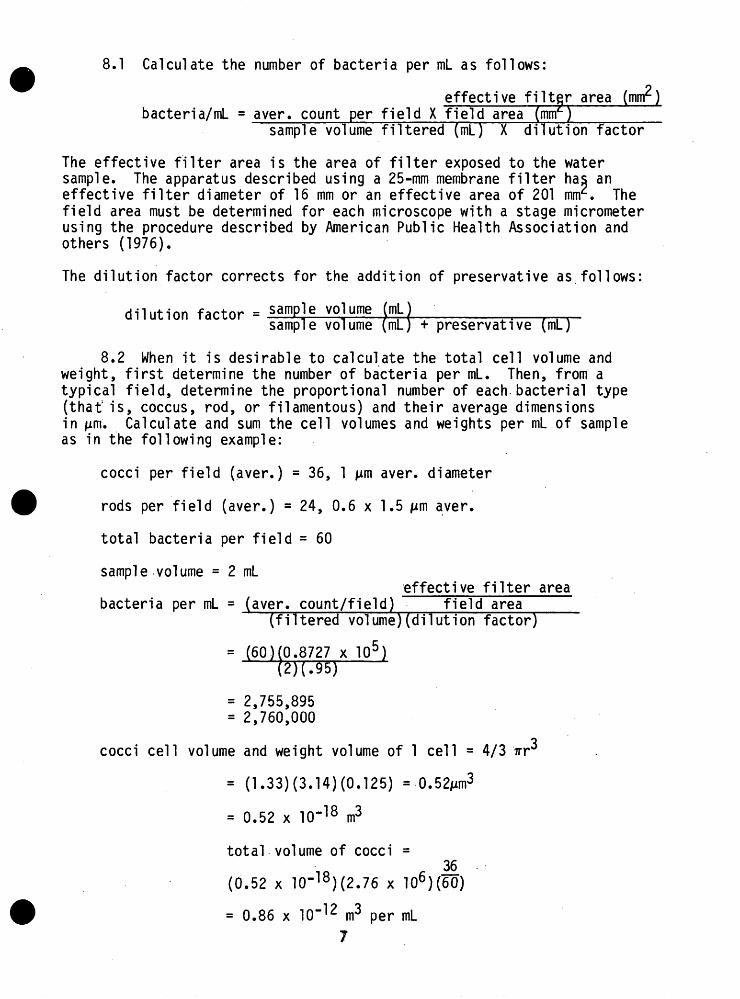
8.1 Calculate the number of bacteria per ml as follows:

effective filter area (mm2 ) bacteria/mL = aver, count per field X field area (mmc )

sample volume filtered (ml)Xdilution factor

The effective filter area is the area of filter exposed to the water sample. The apparatus described using a 25-mm membrane filter has an effective filter diameter of 16 mm or an effective area of 201 mm. The field area must be determined for each microscope with a stage micrometer using the procedure described by American Public Health Association and others (1976).

The dilution factor corrects for the addition of preservative as follows:

dilution factor = sample volume (mlsample volume (mL) + preservativeTmk)

8.2 When it is desirable to calculate the total cell volume and weight, first determine the number of bacteria per ml. Then, from a typical field, determine the proportional number of each bacterial type (that is, coccus, rod, or filamentous) and their average dimensions in jim. Calculate and sum the cell volumes and weights per ml of sample as in the following example:

cocci per field (aver.) = 36, 1 /-im aver, diameter

rods per field (aver.) = 24, 0.6 x 1.5 jim aver,

total bacteria per field = 60

sample volume = 2 mLeffective filter area

bacteria per ml = (aver, count/field) field area___(filtered volume)(dilution factor)

= (60 HO .8727 x IP 5 ) (2)(.95)

= 2,755,895 = 2,760,000

ococci cell volume and weight volume of 1 cell = 4/3 irr*

= (1.33)(3.14)(0.125) = 0.52Mm3

= 0.52 x 10" 18 m3

total volume of cocci =36

(0.52 x 10- 18 )(2.76 x 106 )(60)

= 0.86 x 10" 12 m3 per mL 7

total weight of cocci (g) fi (cocci volume.. nr) (bacterial sp. gr.)(10b g/nr) = (0.86 x 10' IZ )(1.07)(106 ) = 0.92 x 10"b g per mL

The weight and cell volume of the rod shaped bacteria is similarly calcu lated. Results are:

total volume of rods = 0.46 x 10~1 2 m3total weight of rods = 0.49 x 10"6 g

Total cell volume

' = .86 x 10' 12 + Q.46 x 10" 12 m3 = 1.32 x 10~ 12 m3 per ml

Total cell weight

= 0.92 x 10"6 + 0.49 x 10'6 g = 1.41 x 10 b g per ml

9. Report

The bacterial density is reported as cells per mL. Report three significant figures.

10. Precision

The precision is dependent on the density of bacteria in the sample and the amount of nonbacterial debris. For typical samples the precision is approximately _+ 10 percent.

8

References

American Public Health Association and others, 1976, Standard methods for the examination of water and wastewater (14th ed): New York, American Public Health Association, 1993 p.

Dutka, B. J., (ed), 1978, Methods for microbiological analysis of waters, wastewaters, and sediments: Burlington (Canada), Canada Centre for Inland Waters, 288 p.

Hobbie, J. E., Daley, R. J., and Jasper, S., 1977, Use of Nuclepore fil ters for counting bacteria by fluorescence microscopy: Applied and Environmental Microbiology, v. 33, p. 1225-1228.

Kittrell, F. W., 1969, A practical guide to water quality studies of streams: Cincinnati, U.S. Environmental Protection Agency, Publi cation no. CWR-5, 135 p.

PSEUDOMONAS AERUGINOSA (Membrane Filter Method)

(B-0105-79)

Parameter and code: Pseudomonas aeruginosa, MF (colonies/100 mL) 71220

1. Application

The occurrence of Pseudomonas aeruginosa is of increasing concern because it is a frequent causative agent of skin, ear, eye, nose, and throat infections among those engaged in water-contact sports. P. aeruginosa also has often been implicated as the cause of some hospital acquired infections. P. aeruginosa is a natural inhabitant of soil, surface water, and vegetation. The vast majority of the strains identified as P. aeruginosa are nonpathogenic to humans. However, the appearance and~~b~iochemical characteristics of pathogenic strains are indistinguishable from nonpathogenic P. aeruginosa (in the method reported here) so that caution should be observed while handling all Pseudomonas cultures. P. aeruginosa is a gram-negative, rod-shaped bacterium, motile by monotrichous polar flagella. Most strains produce a variety of pigments, some of which are used as a means of identification in this method. A fluorescent greenish-blue pigment and pyocyanin (blue) pigment are the most common but some strains also produce pyorubin, a brownish-red pigment. An incubation temperature of 41.5°C is used because other fluorescent pseudomonads, such as P. fluorescens, will not grow at, or above, 41°C.

The greatest health concern for the presence of P. aeruginosa in the environment has been in water used for swimming. Presently, insufficient work has been done to indicate safe limits of P. aeruginosa in bathing waters. Brodsky and Nixon (1974) reported that 43 percent of the swimming pools studied had<18 P. aeruginosa per 100 mL and 77 percent had a count of <160 P. aeruginosa per 100 ml. The occurrence and pathogenicity of P. aeruginosa in surface waters is not well known except that P. aeruginosa is widely distributed in all waters.

The method is applicable to all waters which do not have high suspended solids content.


A water sample is filtered through a 0.45-jmn pore size membrane filter. The membrane filter is placed on m-PA agar and incubated for 48 hr at 41.5°C. Following incubation, colonies exhibiting typical diffuse brown pigment are counted. Typical colonies may be verified by reaction on skim milk agar.

10

3. Interferences

Suspended materials make it difficult to filter sufficiently large sample volumes to produce statistically valid results. In addition, some suspended material is toxic to bacteria and inhibits their growth. If suspended material is a problem, the multiple tube method described by the American Public Health Association and others (1976) may be used to estimate P. aeruginosa numbers.

4. Apparatus

All materials used in this method must be free of agents that inhibit bacterial growth.

4.1 Water sampling bottle. Many types of bacteriological sampling apparatus are available commercially. Samplers of the Kemmerer or Van Dorn type collect a point sample and may be used. However most of these devices are not autoclavable, and the metallic parts, if present, have bacteriocidal effects. The Niskin sampler consists of a sterile plastic bag which is opened by spring-loaded metal hinges. It is messenger operated and can collect 1-L or 5-L samples (Colwell and others, 1975). A simple sterile bottle sampler can be used in shallow water. The device can be built to fit any size sterilized bottle in common use. As a minimum, a sterile 150-ml or larger glass or plastic bottle may be filled by hand.

4.2 Incubator with temperature of 41.5° +_ 0.5°C.

4.3 Filter-holder assembly, Millipore (XX63 001 20) or equivalent, and syringe and two-way valve, Millipore (XX62 000 35) or equivalent.

4.4 Membrane filters, white, grid, sterile packed, 0.45-um pore size, 47-mm diameter Millipore (HAWG 047 SI), or equivalent.

4.5 Plastic petri dishes with covers, disposable, sterile, 50 X 12 mm, Millipore (PD10 047 00) or equivalent. ,

4.6 Forceps, stainless steel, smooth tips, Millipore (XX62 000 06) or equivalent.

4.7 Microscope, binocular wide-field dissecting-type, Bausch & Lomb (31-26-29-73) or equivalent, with fluorescent lamp, Bausch & Lomb (31-33-63) or equivalent.

4.8 Sterilizer, steam autoclave, Curtin Matheson Scientific (209-536), or Market Forge Sterilmatic, or equivalent.

4.9 Bottles, milk dilution, APHA, Pyrex or Kimax, with screwcaps.

4.10 Pi pets, 1.0-ml capacity, sterilized, disposable, glass or plastic with cotton plugs, Millipore (XX63 001 35) or equivalent, or sterile, disposable, 1.0-ml hypodermic syringes.

11 '

4.11 Propipet, for use with 1.0-, 10.0-, and 11.0-ml pipets.

4.12 Thermometer, with range of at least 40°-100°C, Brooklyn Thermometer Co. (641OY) or equivalent.

4.13 Plastic petri dishes with covers, disposable, sterile, 100 X 15 mm, GSA stock (6640-051-9495) or equivalent.

4.14 Bacteriological transfer needle, Arthur H. Thomas (7010-E15) or equivalent.

4.15 Whirl Pak, 18 oz. Nasco Corp., or equivalent.

4.16 Analytical balance, with sensitivity of 0.1 mg.

4.17 pH meter, Sargent-Welch PBL or equivalent.

5. Reagents

5.1 m-PA agar. The formulation of m-PA agar is shown in Table 1. To prepare m-PA, combine all ingredients except for antibiotics and adjust to pH 6.5 with W NaOH. Sterilize at 121°C at 15 psi (1.05 kg/en/) by autoclaving. Cool to 55-60°C and aseptically readjust to pH 7.1 _+ 0.1. This can be done by removing small aliquots of medium to check the pH after adding IN^ NaOH. If the amounts in Table 1 are followed, approximately 1.1 ml of IN^ NaOH will be needed at this point to attain pH 7.1. After the pH of 7.1 has been maintained, the antibiotics in Table 1 should be added with a gentle swirling motion. The medium is poured into 60-mm diameter petri dishes to a depth of 4 mm (6-8 ml) when the melted medium has cooled at 50°C or less.

5.2 Buffered dilution water. Dissolve 34.0 g potassium dihydrogen phosphate (KHoP04 ) in 500 ml distilled water. Adjust to pH 7.2 with 1 N_ sodium hydroxide (NaOH). Dilute to 1 liter with distilled water. Sterilize in dilution bottles for 20 minutes at 121 °C at 15 psi (1.05 kg/cnr). After opening a bottle of stock solution, refrigerate the unused part. Discard contaminated solutions, indicated by slight turbidity or precipitate. Add 1.2 ml of stock phosphate buffer solution to 1 liter of distilled water containing 0.1 percent Difco peptone (0118) or equi valent. Dispense in milk dilution bottles in amounts that will provide 99 + 2.0 ml after autoclaving at 121°C at 15 psi (1.05 kg/crrr) for 20-10 minutes. Loosen caps or stoppers prior to sterilizing and tighten when bottles have cooled.

5.3 Skim milk agar.

Solution A:

Skim milk, Difco (0032) or equivalent 100 g

Distilled water 500 mL

12

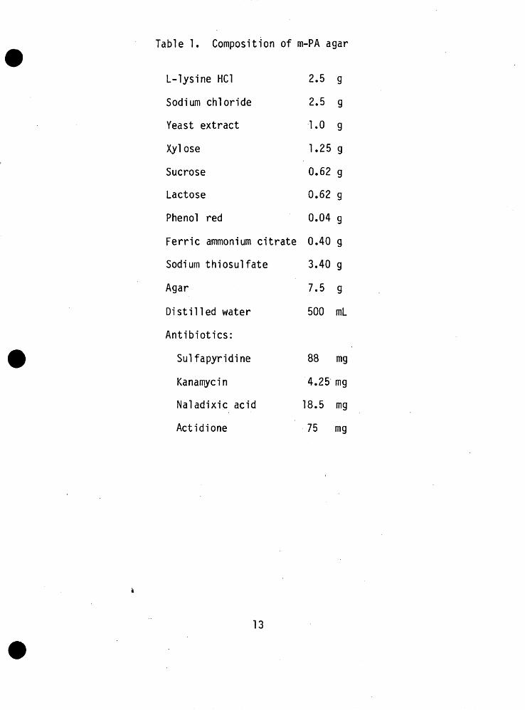
Table 1. Composition of m-PA agar

L-lysine HC1 2.5 g

Sodium chloride 2.5 g

Yeast extract 1.0 g

Xylose 1.25 g

Sucrose 0.62 g

Lactose 0.62 g

Phenol red 0.04 g

Ferric ammonium citrate 0.40 g

Sodium thiosulfate 3.40 g

Agar 7.5 g

Distilled water 500 mL

Antibiotics:

Sulfapyridine 88 mg

Kanamycin 4.25 mg

Naladixic acid 18.5 mg

Actidione 75 mg

13

Solution B:

Nutrient broth 12.5 g

Nad 2.5 g

Agar, Difco (0140) or equivalent 15 g

Distilled water 500 ml

Heat solutions separately to boiling, and dispense in convenient volumes (such as 75 ml_ in 160-mL milk dilution bottles). Sterilize at 121°C at 15 psi (1.05 kg/cnr) for 15 minutes by autoclaving. Cool to approximately 60°C, then combine equal volumes of solution A and B, and pour into 100-mm petri dishes to depth of 4 mm (15 mL). After solidi fication occurs, the plates should be stored in a plastic bag at 2-5°C (refrigerated) for not over 2 weeks. Sterile skim milk agar (solutions uncombined) also may be refrigerated for 2 weeks and can be melted and combined, as needed.

6. Collection

Samples for bacteriological examination must be collected in bottles that have been carefully cleaned and autoclaved for 20 minutes at 121°C at 15 psi (1.05 kg/cnr). Sterilized milk dilution bottles are ideal sample containers. When the sample is collected, ample air space must be left in the bottle to facilitate mixing of the sample by shaking. Care must be taken to avoid contamination of the sample and sample bottle at the time of collection and in the period prior to analysis.

To insure maximum correlation of results, the sample sites and methods used for bacteria should correspond as closely as possible to those selected for chemical and plankton sampling. However, sampling for bacteria at depth is complicated by the requirement to avoid con tamination of the deeper water layers by bacteria carried from shallower depths on the inner walls of the sampler.

The sample collection method will be determined by the study objectives. In lakes, reservoirs, deep rivers, and estuaries, bacterial concentrations may vary transversely, with depth, and with time of day. To collect a surface sample from a stream or lake, open a sterile milk dilution bottle, grasp it near its base, and plunge it, neck downward, below the water surface. Allow the bottle to fill by slowly rotating the bottle until the neck points slightly upward. The mouth of the bottle must be directed into the current. If there is no current, as in the case of a lake, a current should be created artificially by pushing the bottle horizontally forward in a direction away from the hand (American Public Health Association and others, 1976>.

14

To collect a sample representative of the bacterial concentration at a particular depth, use one of the water-sampling bottles discussed in 4.1 above. For small streams, a point sample at a "single transverse position located at the centroid of flow may be adequate.

7. Analyses

7.1 Sterilize filter apparatus. In the laboratory, the funnel and filter base may be wrapped separately in kraft paper packages and sterilized in the autoclave for 15 minutes at 121°C at 15 psi (1.05 kg/cm2 ). Cool to room temperature before use.

Field sterilization of filter apparatus should be in accordance with the manufacturer's instructions but autoclave sterilization in the laboratory prior to the field trip is preferred.

7.2 Assemble filtration equipment and, using sterilized forceps, place a sterile membrane filter over the porous plate of the apparatus, grid side up. Place funnel on filter with care to avoid tearing or creasing the membrane.

7.3 If the volume of sample to be filtered is 10 mL or more, trans fer the measured sample directly onto the dry membrane. For most surface waters, sample volumes of 10, 40, 100 and 200 mL are suggested. Filtration volumes over 100 mL probably will have to be split between 2 or more filters.

If the volume of sample is between 1.0 mL and 10 mL, pour about 20 mL of sterilized buffered dilution water into the funnel before transferring the measured sample onto the membrane. This facilitates distribution of organisms on the filter.

If the volume of original water sample is less than 1.0 mL, proceed as above after preparing appropriate dilutions by adding the sample to a sterile milk dilution bottle in the following amounts:

DilutionVolume of sample added

to 99 mL dilution bottle Filter this volume

1:10 1:100 1:1,000 1:10,000

11.0 mL original sample 1.0 mL original sample 1.0 mL of 1 :10 dilution 1.0 mL of 1:100 dilution

11.0 ml of 1:10 dilution 1.0 ml of 1:100 dilution 1.0 ml of 1:1,000 dilution 1.0 ml of 1:10,000 dilution

NOTE: Use a sterile pi pet or hypodermic syringe for each bottle. After each transfer between bottles, close and shake the bottle vigorously at least 25 times. Diluted samples should be filtered within 20 minutes after preparation.

15

7.4 Apply vacuum and filter the sample. When vacuum is applied with a syringe fitted with a two-way valve, proceed as follows. Attach the filter assembly to the inlet of the two-way valve with plastic tubing. Draw the syringe plunger very slowly on the initial stroke to avoid the danger of airlock before the filter assembly fills with water. Push the plunger forward to expel air from the syringe. Continue until the entire sample has been filtered. If the filter balloons or develops bubbles during sample filtration, dissassemble the two-way valve and lubricate the rubber valve plugs lightly with stopcock grease.

7.5 Rinse sides of funnel twice with 20-30 ml of sterile buffered dilution water while applying vacuum.

7.6 Remove funnel from receptacle and place upside down on a clean surface.

7.7 With flame-sterilized forceps, remove the membrane filter from the filter base and place it on the agar medium in the plastic petri dish, grid side up, using a rolling action at one edge. Use care to avoid trapping air bubbles under the membrane.

7.8 Place top on petri dish and proceed with filtration of the next volume of water. Filter in order of increasing sample volume, rinsing with sterile buffered dilution water between filtrations.

7.9 Clearly mark the lid of each plastic dish indicating location, time of collection, time of incubation, sample number, and sample volume as appropriate. Use a waterproof felt-tip marker or grease pencil.

7.10 Inspect the membrane in each petri dish for uniform contact with the medium. If air bubbles are present under the filter (indicated by bulges), remove the filter with sterile forceps and roll onto the medium again.

7.11 Close the plastic petri dish by firmly pressing down on the top.

7.12 Incubate the petri dishes with filters in an inverted position (agar and filter at the top) for 48 + 2 hours at 41.5 + 0.5°C. If a waterbath incubator is used, the petri dishes should either be taped to prevent water entry or the dishes may be put into Whirl Pak or equivalent plastic bags. The dishes must be incubated below the water surface in any case.

7.13 After incubation, remove petri dish lids and count typical colonies at 15X magnification. Angle of illumination is not critical. Pseudomonas aeruginosa colonies are dark brown with an irregular margin and are almost flat. A light brown pigment diffusing radially away from the colony is usually visible. Plates having between 20 and 80 P. aeruginosa colonies are considered to be ideal for counting purposes and should be used for calculation, if possible.

16

7.14 Some of the colonies counted as P. aeruginosa should be confirmed by determining growth on skim milk agar. Sterilize an inoculating needle by heating the wire in a burner flame until red hot, then allow to cool for 10 sec in air. The entire length of wire must be sterilized. Remove a small portion of a colony with the sterilized inoculating needle and lightly streak the skim milk agar surface. Several such transfers may be made to each plate, sterilizing the needle between each inoculation. Every inoculation should have appropriate notation to identify the source.

Invert and incubate each inoculated plate at 20-35°C for 24-48 hr. P. aeruginosa causes casein hydrolysis (clearing of the agar) where growth occurs. A yellow-green diffusible pigment should be visible when the plate is viewed from the side.

7.15 Autoclave all cultures at 121°C at 15 psi (1.05 kg/cm2 ) for 15 min before discarding.

8. Calculations

8.1 For colony counts between the ideal of 20 and 80, use the formula:

Pseudomonas aeruginosa (colonies/100 ml)

_ P. aeruginosa colonies x 100 sample volume filtered (ml)

8.2 Counts less than the ideal of 20 colonies or greater than 80 colonies per filter should be reported as the number per 100 ml, followed by the statement, "Estimated count based on nonideal colony count."

8.3 If no filters have characteristics P. aeruginosa colonies, calculate a number as in 8.1 assuming that the largest sample volume filtered had one P. aeruginosa colony. Report as less than that calcu lated number per 100 ml.

8.4 If all filters have colonies too numerous to count, a minimum estimated value can be reported. Assume a count of 80 P. aeruginosa colonies on the smallest filtered volume, then calculate according to the formula in 8.1. Report as greater than the calculated value.

8.5 Sometimes two or more filters of a series will produce colony counts within the recommended counting range. Colony counts should be made on all such filters. The method for calculating and averaging is as follows:

17

Volume filter 1 Colony count filter 1+ Volume filter 2 + Colony count filter 2

Volume sum Colony count sum

Pseudomonas aeruginosa (colonies/100 ml)

- colony count sum x 100 vol. sum (ml)

NOTE: Do not calculate the P. aeruginosa colonies per 100 ml for each volume filtered and then average the results. If a large filtered volume was split between several filters, the count should be made as in 8.5. Such counts are considered to be in the ideal range if the sum of the colonies is between 20 and 80 colonies.

9. Report

The Pseudomonas aeruginosa density is reported as Pseudomonasaeruginosa colonies per 100 ml. For values less than 10, report wholenumbers; for values 10 or more, report two significant figures.

10. Precision

Carson and others (1975) reported a mean recovery of 95 percent of naturally occurring Pseudomonas aeruginosa using m-PA agar.

18

References

American Public Health Association and others, 1976, Standard methods for the examination of water and wastewater (14th ed.): New York, American Public Health Association, 1193 p.

Brodsky, M. H., and Nixon, M. C., 1974, Membrane filter method for the isolation and enumeration of Pseudomonas aeruginosa from swimming pools: Applied Microbiology, v. 27, no. 5, p. 938-943.

Carson, L. A., Petersen, N. J., Favero, M. S., Doto, I. L., Coll ins, D. E., and Levin, M. A., 1975, Factors influencing detection and enumeration of Pseudomonas aeruginosa by most-probable-number and membrane filtration techniques: Applied Microbiology, v. 30, no. 6, p. 935-942.

Colwell, R. R., Sizemore, R. K., Carney, J. F., Morita, R. Y., Nelson, J. D., Jr., Pickar, J. H., Schwarz, J. R., Van Valkenburg, S. D., Walker, J. D., and Wright, R. T., 1975, Marine and estuarine micro biology laboratory manual: Baltimore, University Park Press, 96 p.

Goerlitz, D. F., and Brown, Eugene, 1972, Methods for analysis of organic substances in water: U.S. Geological Survey Techniques Water-Resources Investigations, book 5, chap. A3, 40 p.

19

PHYTOPLANKTON

INVERTED MICROSCOPE METHOD (B-l520-79) jy

Parameter and code: Phytoplankton, total (cells/nt) 60050

1. Application

The method is suitable for all waters.


Taxonomic and numerical assessment of natural populations of phytoplankton require direct microscopic examination. The inverted microscope method permits the observation of the phytoplankton in an aliquot of water at high-power magnification without disrupting or crushing the delicate organisms.

The phytoplankton are concentrated by settling to the bottom of a sample container or a vertical-tube sedimentation apparatus (Utermohl, 1931, 1936, 1958; Lovegrove, 1960). Lund, Kipling, and LeCren (1958) reported that all known algae can be settled.

After setting, an aliquot of phytoplankton sample is poured into a plankton chamber or a sedimentation apparatus. The algae settle onto a microscope cover slip which forms the bottom of the chamber or apparatus, and the settled algae are observed from beneath using an inverted micro scope. Because this method permits use of the high dry and oil-immersion objectives on the microscope, very small forms can be identified and enumerated.

3. Interferences

The method is generally free of interferences. Suspended sediment may obscure microorganisms in a sample. Previously used parts of the sedi mentation apparatus must be cleaned thoroughly to remove adherent diatoms and other material, especially from the bottom surfaces. Convection cur rents and air bubbles in the apparatus can interfere with sedimentation.

4. Apparatus

4.1 Inverted microscope, Zeiss Invertoscope D, or equivalent.

4.2 Ocular micrometer, Whipple grid, Bausch & Lomb (31-16-13) or equivalent.

I/ supercedes method B-1520-77 (TWRI, Book 5, Chapter A4, 1977, p. 97-99).

20

4.3 Plankton chamber, 26 X 76-mm glass slide with 12-mm circular hole covered by cementing no. 1-1/2 cover slip to slide, and a No. 1-1/2 cover slip for top of chamber.

4.4 Sedimentation apparatus of the type described by Lovegrove (1960) (see fig. 14, TWRI, Bk. 5, Chap. A4, 1977, p. 98), 8-cm high, 25-mL capacity, Scott Instruments, Seattle, Wash., or equivalent. Other sizes may be needed for some types of samples (see 7.3 below).

4.5 Cover slip, 22-mm diameter, No. 1 and No. 1-1/2.

4.6 Rubber cement for attaching cover slip to the counting chamber.

4.7 Sample containers, linear polyethylene bottles, 1,000-ml capacity.

4.8 Water-sampling bottle, Wildlife Supply Co. (1510 or 1920); Scott Instruments, Seattle, Wash.; Foerst Mechanical Specialities Co., Improved Water Sampler, Kemmerer-type; or equivalent. Depth-integrated samplers are discussed by Guy and Norman (1970).

4.9 Cotton swabs.

4.10 Vacuum grease.

4.11 Pi pet, serological, 1 ml.

4.12 Balance, with automatic tare, Sartorius or equivalent.

5. Reagents

5.1 Cupric sulfate solution, saturated. Dissolve 21 g CuS04 in 100 mL distilled water.

5.2 Formaldehyde-cupric sulfate solution. Mix 1-L of 40 percent aqueous formaldehyde, Fisner Scientific No. F-78, or equivalent, with 1 ml of solution 5.1.

5.3 Detergent solution, 20 percent. Dilute 20 ml liquid detergent (Liqui-Nox, C6308-2, phosphate free, or equivalent) to 100 ml with dis tilled water.

5.4 Lugol *s solution. Dissolve 10 g iodine crystals and 20 g potas sium iodide in 200 mL distilled water. Add 20 mL glacial acetic acid a few days prior to using; store in amber glass bottles (Vollenweider, 1969).

6. Collection

A phytoplankton sample consists of a sample of water, usually 1 liter. To insure maximum correlation of results, the sample .sites and methods used for phytoplankton should correspond as closely as possible to those selected for chemical and bacteriological sampling.

21

The sample collection method will be determined by the study objec tives. In lakes, reservoirs, deep rivers, and estuaries, phytoplankton abundance may vary transversely, with depth, and with time of day. To collect a sample representative of the phytoplankton density at a parti cular depth, use a water-sampling bottle. To collect a sample represen tative of the entire flow of a stream, use a depth-integrated sampler (Guy and Norman, 1970; Goerlitz and Brown, 1972). For small streams, a depth-integrated sample or a point sample at a single transverse posi tion located at the centroid of flow may be adequate.

Preserve sample as follows: To each 1,000 mL of sample, add 40 ml of 37-40 percent aqueous formaldehyde solution (100 percent Formalin), 5 mL of 20 percent detergent solution, and 1 mL of cupric sulfate solution. This preservative maintains cell coloration and is effective indefinitely.

Many biologists consider Lugol's solution to be the best plankton preservative. It has been effective for at least 1 year (Weber, 1968); it facilitates sedimentation of cells and maintains fragile cell struc tures, such as flagella. If Lugol's solution is used as a preservative, add 1 ml Lugol's solution to each 100 mL of sample. Store the preserved samples in the dark.

7. Analysis

7.1 If using the sedimentation apparatus, proceed to 7.5. If using the plankton chamber, proceed as follows: If concentration is necessary, allow the sample to settle undisturbed in the sample container for 4 hours per centimeter of depth to be settled. After settling, weigh the sample container on an analytical balance. Record the tare weight.

7.2 Carefully siphon the supernatant to avoid disturbance of the settled material. Place sample container with remaining sample on balance and weigh. The reduction in weight (in grams) is equivalent to the number of milliliters of supernatant removed. The same method can be used to obtain the volume of concentrate.

7.3 Mix the concentrated sample thoroughly (but not vigorously) and pi pet an appropriate volume into each of two plankton chambers. Slide cover slip into place.

7.4 Place the plankton chamber on the mechanical stage of a cali brated microscope. Proceed to 7.10.

7.5 To prepare the sedimentation apparatus, cement a no. 1 glass cover slip to the bottom of the lower slide to form the bottom of the counting chamber. When dry, remove the excess rubber cement from the inside of the counting chamber with a knife.

22

7.6 Test for leaks: Coat the underside of the upper slide with vacuum grease, and press onto the lower slide to form a watertight seal. Assemble the apparatus and fill with distilled water so that the meniscus bulges slightly above the top of the sedimentation tube. Slide the cap over the top to seal the tube. Let stand overnight and check for water loss in the morning.

7.7 If no leaks are detected, thoroughly mix a sample by inverting it at least 40 times, and then fill the sedimentation apparatus and apply the cap as described in 7.6. Allow 4 hours settling time per 1 cm of sedimentation tube length. The volume of sample is dependent on the density of algae. In plankton-scarce waters, 100 ml of sample may be required; in more fertile waters, 25 mL or less of sample may be suffi cient. The 25-mL volume is most commonly used. The samples may be diluted, if necessary.

Note: Air bubbles on the sides of the chamber tube can be prevented if the water sample and the sedimentation apparatus are at the same temperature when the sample is introduced. The apparatus should be main tained at a constant temperature to avoid convection currents which can interfere with settling.

7.8 After settling, isolate the algae in the counting chamber from the remainder of the apparatus. To separate the sedimentation tube and upper slide from the lower slide and counting chamber, move the sedimen tation tube to one side splitting the water column. Remove the tube cap and siphon or pi pet the supernatant from the chamber. Remove the empty sedimentation tube.

7.9 Remove the lower slide with the counting chamber from the holder. Place the cap over the top of the counting chamber to form a closed cell. If an air bubble remains under the cap, tease it to one side of the chamber and carefully add distilled water to fill the void. Replace the tube cap and put the slide on the inverted microscope.

7.10 Count and identify the total number of algal cells (at X 200-300 magnification) in randomly chosen fields. In making the counts, enumerate all forms that intersect two of the borders of the grid, but do not count those that intersect the opposite borders. If a large number of colonies appear within the field, determine the average number of cells in an average size colony and multiply by the number of colonies present. Simi larly, tabulate the numbers and lengths of trichomes of blue-green algae in each grid and determine the average number of cells per unit length of trichome. Count all algae containing any part of a protoplast as having been living at the time of collection. Count a minimum of 100 units (unit = one filament, one colony, or one unicellular alga) or 250 fields (at X 200-300) whichever is obtained first. For concentrated samples count a minimum of 10 fields.

23

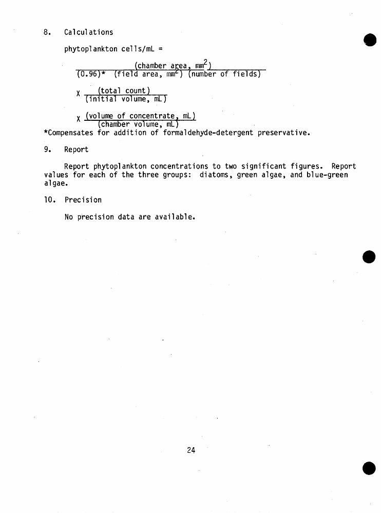
8. Calculations

phytoplankton cells/ml =

p (chamber aea, ronr)(0.96)* (field area, mnf) (number of fields)

X (total count) (initial volume, ml)

X (volume of concentrate. mL)(chamber volume, ml)

Compensates for addition of formaldehyde-detergent preservative.

9. Report

Report phytoplankton concentrations to two significant figures. Report values for each of the three groups: diatoms, green algae, and blue-green algae.

10. Precision

No precision data are available.

24

References

Goerlitz, D. F., and Brown, Eugene, 1972, Methods for analysis of organic substances in water: U.S. Geological Survey Techniques Water-Resources Investigations, book 5, chap. A3, 40 p.

Guy, H. P., and Norman, V.- W., 1970, Field methods for the measurement of fluvial sediments: U.S. Geological Survey Techniques Water- Resources Investigations, book 3, chap. C2, 59 p.

Lovegrove, T., 1960, An improved form of sedimentation apparatus for use with an inverted microscope: Conseil Permanent Internationale Ex- plor. Mer. Journal, v. 25, no. 3, p. 279-284.

Lund, J. W. G., Kipling, C., and LeCren, E. D., 1958, The inverted micro scope method of estimating algal numbers and the statistical basis of estimations by counting: Hydrobiologia, v. 11, p. 144-170.

Utermohl, H., 1931, Uber das umgekehrte Mikroskop: Archiv Hydrobiologie Planktonkunde, v. 22, p. 643-645.

_1936, Quantitative Methoden zur Untersuchung des Nannoplankton:Abderhalden Handbuch biologiae Arbeiten Methologiae, Abt. 2, v. 2, p. 1879-1937.

J958, Zur Vervollkommnung der quantitativen Phytoplankton-MethodikInternationale Verein Limnologie Mitteilung, no. 9, 38 p.

Vollenweider, R. A., ed., 1969, A manual on methods for measuring primary production in aquatic environments: International Biological Pro gramme Handbook 12, 213 p.; Oxford and Edinburgh, Blackwell Scientific Publishers.

Weber, C. I., 1968, The preservation of phytoplankton grab samples: American Microscopical Society Transactions, v. 87, p. 70-81.

25

SESTON

GLASS-FIBER FILTER-METHOD (B-3401-79)*/

Parameters and codes: Seston, dry weight (mg/1) 71100Seston, ash weight (mg/1) 71101

1. Application



A known volume of water is passed through a tared glass-fiber filter to remove the particulate matter. The increase in weight of the filter after drying at 105°C is a measure of the dry weight of particulate material in the sample. After ashing the residue at 500°C, the difference between dry weight and ash weight is taken as the weight of particulate organic matter in the sample.

3. Interferences

Although the method is generally free from interferences, it is essential that bottles and sampling equipment be clean and that samples, filters, and funnels be protected from dust. Filtration should be at reduced pressure to avoid rupture and loss of cell contents of fragile organisms. Saline samples must have the salts washed from the filter residues to prevent erroneous weight values.

4. Apparatus

4.1 Glass filters, Whatman, GF/C grade, or equivalent, 47-mm-diameter disks. For best results all filters for a series of samples, inclu ding control filters, should be from the same box and should have a tare weight within about 10 mg on 70- to 100-mg weights.

4.2 Filter funnel, vacuum, 1,200-mL capacity, stainless steel, Gelman Instrument Co. (Parabella) or equivalent.

4.3 Filter flask, 1,000 or 2,000 ml_. For field use a polypropylene flask, Bel-Art Products (H-38941), Nalgene Labware (4101), or equivalent is suggested.

2 Supercedes method B-3401-77 (TWRI, Book 5, Chapter A4, 1977, p. 123-125).

26

4.4 Source of vacuum for filtration: a water-aspirator pump or an electric vacuum pump for use in the laboratory; a hand-held vacuum pump with gauge, Edmund Scientific Co. (71,301) or equivalent, for use in the field.

4.5 Manostat with mercury and calibration equipment to regulate the filtration suction at not more than 300 to 350 mm of mercury when filtering with an aspirator or an electric vacuum pump.

4.6 Forceps, stainless steel, smooth tip, Millipore (XX62 000 06) or equivalent.

4.7 Balance capable of weighing to at least 0.1 mg.

4.8 Plastic petri dishes with covers for filter storage, Millipore (PD10 047 00) or equivalent.

4.9 Desiccator containing silica gel or anhydrous calcium sulfate.

4.10 Alumni urn foil, laboratory grade.

4.11 Drying oven, thermostatically controlled for use at 105°C.

4.12 Muffle furnace, for use at 500°C.

4.13 Graduated cylinders of a size suitable to the volume of water to be filtered. Plastic cylinders, BelArt Products, Nalgene Labware, or equivalent of 500- and 1,000-mL capacity are convenient for field use.

4.14 Water-sampling bottle, Wildlife Supply Co. (1510 or 1920); Scott Instruments, Seattle, Wash.; or Foerst Mechanical Specialties Co. (Improved Water Sampler, Kemmerer-type), or equivalent. Depth-integrated samplers are discussed in Guy and Norman (1970).

4.15 Sample containers, plastic bottles, 1-liter capacity.

5. Reagents

5.1 Mercuric chloride solution, 1 ml containing 40 mgHg . Dissolve 55.0 g HgCl2 in distilled water and dilute to 1,000 ml.

5.2 Distilled water. Filter if in doubt as to the freedom from particles.

6. Collection

The sample-collection method will be determined by the study objectives. In lakes, reservoirs, deep rivers, and estuaries, seston abundance may vary transversely and with depth (Patten and others, 1966). To collect a sample representative of the seston at a particular depth, use a water-sampling

27

bottle (figs. 11 and 12). To collect a sample representative of the entire flow of a stream, use a depth-integrating sampler (Guy and Norman, 1970; Goerlitz and Brown, 1972). For small streams, a depth-integrated sample or a point sample at a single transverse position located at the centroid of flow may be adequate. Study design, collection, and statistics for streams, rivers, and lakes are described in Federal Working Group on Pest Management (1974).

Adjust the sample volume to the amount of suspended material present. Very clear waters will require 3 or 4 liters of sample; waters with a high sediment or phytoplankton content may require only 500 mL or less. Filter the maximum volume that will not clog the filter.

Seston samples should be filtered as described in sections 7.9 and 7.10 below, immediately after collection. Record the mesh size of pre- filter, if used. Record the volume of water filtered. The filters should be thoroughly dried or stored in tightly closed plastic petri dishes at 1°-4°C (do not freeze) until ovendrying. Samples that cannot be filtered without delay should be preserved with 40 mg hkr /I (1 roL of the mercuric chloride solution per liter of sample). This method for seston preser vation will stabilize the seston content of samples for at least 8 days. However, the results of analyses of preserved samples are not necessarily the same as those obtained by immediate filtration.

7. Analysis

7.1 Arrange the required number of glass filters without overlay onto the shiny side of aluminum foil and heat to 450°-500°C for 30 minutes. Do not allow the temperature to exceed 500°C. This preparation hardens the filters and removes any organic matter. About 20 filters is a con venient number with which to work.

7.2 Designate at least 10 percent of the filters as controls. For large batches use every 10th filter as a control; for small batches use a filter at the beginning and one at the end as controls. The treatment of control filters is identical to that of the test filters except that no water is filtered through them.

7.3 Handle the cooled filters very carefully using clean, smooth tip forceps to avoid fraying the fibers. Transfer the filters including the controls to a shallow container of distilled water for 5 minutes. Allow about 100 mL of water for each filter.

7.4 With forceps, transfer the filters to aluminum foil, after gently shaking off excess water. Dry the filters in an oven at 105°C for 30 minutes. Cool to room temperature in a desiccator.

Note: Because of the difficulty of marking glass filters, it is necessary to keep track of individual filter disks throughout the remaining steps. The disks should be placed on the aluminum foil in a definite sequence and, whenever possible, each disk should be kept in a numbered container.

28

7.5 Weigh each filter to the nearest 0.1 mg as rapidly as possible, and record this initial (tare) weight value. Close the desiccator tightly after each removal. Store the tared filters in numbered plastic petri dishes until needed.

7.6 When a sample is to be filtered, place a tared filter disk, wrinkled surface upward, on a membrane-filtere apparatus. A small slip of aluminum foil under the edge of the disk facilitates removal of the wet filters.

7.7 With vacuum applied, wet the filter with distilled water to seat the disk on the filter base plate.

7.8 Measure out a suitable amount of thoroughly mixed sample into a graduated cylinder. Complete mixing of the sample is essential prior to measuring. Pour the sample into the filter funnel and filter using a manostat or other suitable method to control vacuum to 300-350 mm (about 12 in.) of mercury (about 6 psi).

7.9 With vacuum on, wash the filter and funnel three times with 5-10 ml volumes of distilled water allowing the filter to suck "dry" between each wash.

7.10 Disconnect the vacuum and, with smooth tip forceps, remove the wet filter to the shiny side of aluminum foil. The filters may be stored at 1°-4°C in numbered petri dishes at this stage, if necessary.

7.11 Dry the filters in an oven at 105°C for 1 hour. Include at least two control filters from 7.5 above in this drying step for each batch of sample filters.

7.12 Place the filters in a desiccator, cool, and reweigh each disk rapidly to the nearest 0.1 mg as in 7.5 above. Include the control filters from 7.11. These values are used to calculate dry weight.

7.13 Again place the filters with their dried residue and the control filters on the shiny side of aluminum foil and heat in a muffle furnace at 500°C for 30 minutes.

7.14 Place the filters in a desiccator, cool, and reweigh each filter rapidly to the nearest 0.1 mg as in 7.5 above. Include the control filters from 7.13. These values are used to calculate the ash weight.

8. Calculations

29

8.1 Dry weight of seston (mg/L)

dry weight of filter and residue (mg) - _ ___tar weight of filter (mg)_____

volume of sample (liters

- blank correction (mg)

where blank correction (mg) = mean weight of control filters in mg (from 7.12) - mean weight of control filters in milligrams (from 7.5).

The blank correction value may be positive or negative, but should not exceed about 0.5 mg.

8.2 Ash weight of seston (mg/L)

ignition weight of filter and residue (mg) - _ ______tare weight of filter (mg) ____

volume of sample (liters)

- blank correction (mg)

where blank correction (mg) = mean weight of control filters in mg (from 7.14) - mean weight of control filters in milligrams (from 7.5).

The blank correction value may be positive or negative, but should not exceed about 0.5 mg.

8.3 Volatile or organic weight of seston (mg/L) = dry weight of seston (mg/L) - ash weight of seston (mg/L).

9. Report

Report seston as follows: Less than 1 mg/L, one significant figure; 1 mg/L and above, two significant figures.

10. Precision

No numerical precision data are available.

30

References

Banse, Karl, Falls, C. P., and Hobson, L. A., 1963, A gravimetric method for determining suspended matter in sea water using Millipore filters: Deep-Sea Research, v. 10, p. 639-642.

Federal Working Group on Pest Management, 1974, Guidelines on sampling and statistical methodologies for ambient pesticide monitoring: Washington, D.C., Federal Working Group on Pest Management, 59 p.

Goerlitz, D. F., and Brown, Eugene, 1972, Methods for analysis of organic substances in water: U.S. Geol. Survey Techniques Water-Resources Inv., book 5, chap. A3, 40 p.

Guy, H. P., and Norman, V. W., 1970, Field methods for the measurement of fluvial sediments: U.S. Geol. Survey Techniques Water-Resources Inv., book 3, chap. C2, 59 p.

Jerlov, N. G., 1968, Optical oceanography: New York, Elsevier Pub. Co., 194 p.

Maciolek, J. A., and Tunzi, M. G., 1968, Microseston dynamics in a simple Sierra Nevada lake-stream system: Ecology, v. 49, no. 1, p. 60-75.

Moss, Brian, 1970, Seston composition in two freshwater pools: Limnology and Oceanography, v. 15, no. 4, p. 504-513.

Patten, B. C., Young, D. K., and Roberts, M. H., Jr., 1966, Verticaldistribution and sinking characteristics of seston in the Lower YorkRiver, Virginia: Chesapeake Sci., v. 7, no. 1, p. 20-29.

Reed, D. F., and Reed, E. B., 1970, Estimates of seston crops by filtration with glass fiber discs: Fisheries Research Board Canada Jour., v. 27, no. 1, p. 180-185.

Strickland, J. D. H., and Parsons, T. R., 1968, A practical handbook of seawater analysis: Fisheries Research Board Canada Bull. 167, 311 p.

31

PERIPHYTON

GRAVIMETRIC METHOD FOR BIOMASS (B-3520-79) _3/

pParameters and codes: Periphyton, biomass, dry weight, total (g/nr) 00573Periphyton, biomass, ash-free weight (g/nr) 00572

1. Application

The method quantifies all organisms in the periphyton community. It is suitable for all waters.


Samples of the periphyton community are collected from known areas of artificial or natural substrates. The dry weight and ash-free weight are determined.

3. Interferences

Inorganic matter in the sample will cause erroneously high dry and ash weights; nonliving organic matter in the sample will cause erroneously high dry and ash-free weights.

4. Apparatus

4.1 Artificial substrates made of glass slides, Plexiglas, polyethylene strips, or other materials.

4.2 Collecting devices for the removal of periphyton from natural substrates.

4.3 Scraping devices. Razor blades, stiff brushes, spatulas, or glass slides are useful for removing periphyton from artificial substrates. The edge of a glass microscope slide is excellent for scraping periphyton from hard flat surfaces (Tilley, 1972). A putty knife is excellent for scraping periphyton from plastic strips.

4.4 Sample containers of glass or plastic suitable for the types and sizes of samples. Tightly sealing plastic bags are useful containers for artificial substrates or for pieces of natural substrate. Do not use glass containers for samples to be frozen.

3/ supercedes method B-3520-77 (TWRI, Book 5, Chapter A4, 1977, p. 133-134)

32

4.5 Porcelain crucibles.

4.6 Balance capable of weighing to a precision of at least 1 mg.



4.9 Desiccator containing silica gel or anhydrous calcium sulfate.

4.10 Forceps or tongs.

4.11 Filtration apparatus, non-metallic with vacuum.

4.12 Glass fiber filters, 47 mm, Gelman 61631 type A/E, or equivalent.

5. Reagents

5.1 Distilled water.

6. Collection

6.1 The sample sites should correspond as closely as possible to those selected for chemical, biological, and microbiological sampling, so that there is maximum correlation of results.

6.2 Artificial substrates. Place a suitable artificial substrate in the water body under study and attach it to a supporting object. The sub strates must be submerged but may be near the surface of the water or at any other appropriate depth. In lakes, the substrates are usually suspended at various depths. In lakes and streams, the substrates may be attached to natural objects such as submerged trees, stumps, logs, or boulders or they may be attached to stakes driven into the bottom. Floating samplers may be used. The artificial substrates must be exposed to the light so that photosynthesis can take place, and they should be located so that damage to the apparatus by floating debris is minimized. Vandalism is a common problem and placing the substrates away from frequently traveled areas is advisable. The length of time required for colonization of the substrates by periphyton will depend upon the season, water temperature, light and nutrient availability, arid other factors. Neal, Patten, and DePoe (1967) found that the maximum accumulation of periphyton biomass on polyethylene strips occurred in about 2 weeks. Nielson (1953) exposed his slides for 20-30 days. Exposure probably should be at least 14 days, but this will vary and must be determined for each season and water type.

After sufficient colonization of periphyton, indicated by visible green or brown growth, remove the artificial substrate from the water. Periphyton may be scraped from the substrate in the field or in the laboratory, as described in 4.3 above. Place the scrapings or the entire slide in a suitable container, label, and transport to the laboratory as rapidly as possible. Immediately proceed to 7.1 below, or if ovendrying cannot be started, air-dry or freeze the sample. Storage should not exceed 2 weeks.

33

6.3 Natural submerged substrates often contain periphyton, a known area of which can be sampled quantitatively. Several devices for removing periphyton from a known area of natural substrates are shown in figure 19 of TWRI, Book 5, Chapter A4, 1977, p. 129. The instrument used by Douglas (1958) consists of a broadnecked polyethylene bottle with the bottom removed. The neck of the bottle is held tightly against the surface to be sampled and the periphyton inside the enclosed area is dislodged from the substrate with a stiff nylon brush. The periphyton is removed from the bottle with a pipet. Ertl's (1971) apparatus consists of two concentric metal or plastic cylinders separated with spacers. The space between the cylinders is filled with modeling clay and the sampler is pressed firmly against the substrate to be sampled. With a blunt stick or metal rod the clay is forced down onto the substrate so as to isolate the sampling area of the inner circle. The periphyton within the inner circle is dislodged with a stiff brush and removed with a pipet. Stockner and Armstrong (1971) sampled periphyton with a plastic hypodermic syringe which had a toothbrush attached to the end of the syringe piston. With the barrel of the syringe held tightly against the substrate, the piston is pushed in until the brush contacts the periphyton. The piston is then rotated several times to dislodge the periphyton and then is withdrawn, pulling the periphyton up with it. A glass plate is immediately placed under the end of the barrel and the syringe inverted. Small holes drilled through the base of the barrel facilitate periphyton collection (J. G. Stockner, written commun., March 1972). Place the scrapings or the entire slide in a suitable container, label, and transport to the laboratory as rapidly as possible. Immediately proceed tp 7.1 below, or if ovendrying cannot be started, air-dry or freeze the sample. Storage should not exceed 2 weeks.

7. Analysis

7.1 Obtain the tare weight of a crucible containing a glass fiber filter by holding at 500°C for about 20 minutes, cooling to room tempe rature in a desiccator, and weighing to the nearest mg.

7.2 Filter the water in the sample bottle and the scrapings from the periphyton strip. Dry at 105°C to a constant weight. Cool crucibles containing dried periphyton to room temperature in a desiccator before weighing. Weigh as rapidly as possible to decrease moisture uptake by the dried residue. These values are used to calculate dry weight.

7.3 Place the crucible containing the dried residue in a muffle furnace for 1 hour at 500°C. Cool to room temperature.

7.4 Moisten the periphyton ash with distilled water and again ovendry at 105°C to constant weight as described in 7.2. These weight values are used to calculate ash weight.

34

8. Calculations

8.1 Dry weight of periphyton (g/m2 )

dry wt of crucible and residue (g) = ____- tare wt of crucible (g)

P area of scraped surface (nr)

8.2 Ash weight of periphyton (g/m2 )

ash wt of crucible and residue (g) = ____- tare wt of crucible (g)

area of scraped surface (nr)P 8.3 Ash-free weight of periphyton (g/m )

= dry weight (g/m2 ) - ash weight (g/m2 )

9. Report

Report biomass as grams per square meter to three significant figures.

10. Precision

No numerical precision data are available.

35

References

Douglas, Barbara, 1958, The ecology of the attached diatoms and other algae in a small stony stream: Journal Ecology, v. 46, p. 295-322.

Ertl, Milan, 1971, A quantitative method of sampling periphyton from rough substrates: Limnology and Oceanography, v. 16, no. 3, p. 576-577.

Neal, E. C., Patten, B. C., and DePoe, C. E., 1967, Periphyton growth on artificial substrates in a radioactively contaminated lake: Ecology, v. 48, no. 6, p. 918-923.

Nielson, R. S., 1953, Apparatus and methods for the collection of attached materials in lakes: Progressive Fish-Culturist, v. 15, no. 2, p. 87-89.

Stockner, J. G., and Armstrong, F. A. J., 1971, Periphyton of the experi mental lakes area, Northwestern Ontario: Fisheries Research Board Canada Journal, v. 28, p. 215-229.

Til ley, L. J., 1972, A method for rapid and reliable scraping of periphyton slides: U.S. Geological Survey Professional Paper 800-D, p. D221-D222.

36

INVERTED MICROSCOPE METHOD FOR THE IDENTIFICATION AND ENUMERATION OF PERIPHYTIC DIATOMS

(B-3545-79)

Parameter and code: Diatoms, total, periphyton (number/mm2 ) 81804

1. Application

The method is suitable for all waters. The diatoms are cleared, making identification to species possible. Reliable quantitative enume ration is possible after the diatoms are separated from one another and from extracellular organic matter.


Periphytic diatoms are collected by scraping from their substrate. Organic components including gelatinous stalks and matrices and celluar components in the diatoms are decomposed by oxidation. The diatoms in a sample are concentrated and a permanent mount is prepared from a 0.1-ml aliquot. The mount is examined microscopically for the purpose of iden tification and tabulation, and the cleared diatoms are placed in a chamber for enumeration.

3. Interferences

Large amounts of sediment associated with the periphyton may obscure the diatoms in the counting chamber. Sediment and other particulate matter, including salt crystals and carbonaceous residues, interfer with slide- mount perparation.

4. Apparatus

4.1 Artificial substrates, made of glass slides, Plexiglass polyethylene strips, or other suitable materials.

4.2 Sample containers of glass or plastic suitable for the types of sample.

4.3 Scraping devices. Razor blades, stiff brushes, spatulas, or glass slides are useful for removing periphyton from artificial or natural substances.

4.4 Microscope, inverted, with planapochromatic objectives (20-100x) and linear and grided ocular micrometer.

4.5 Microscope, compound binocular, withplanopochromatic objectives (20-100x) and a linear micrometer.

37

4.6 Counting chamber. 25 x 76-cm glass slide with 12-mm circular hole covered by cementing a no. 1 1/2 cover slip to slide, and a no. 1 1/2 cover slip for top of chamber.

4.7 Vial , 10-mL, glass, disposable (for reference sample).

4.8 Water aspirator.

4.9 Cylinders, graduated, with glass stopper, (100, 250, 500 ml), Corning no. 3360, or equivalent.

4.10 Microspatula, 0.1 gram.

4.11 Hotplate, thermostatically controlled to 510°C (950°F), Corning PC-35 electric hotplate or equivalent. It is convenient to have a second hotplate for operation at about 93°-121°C (200°-250°F).

4.12 Cover glass squares, 18 x 18-mm, no. 1-1/2 and microscope slides, glass, 76 x 25-mm, frosted end.

5. Reagents

5.1 Formaldehyde solution, 4 percent. Dilute 10 ml of 37-40 percent aqueous formaldehyde solution (Formalin) to 100-mL with distilled water.

5.2 Immersion oil , Cargille.'s nondrying type A, Scientific Products M6002-1, or equivalent.

5.3 Hyrax , high-refraction index-mounting medium, Custom Research and Development, Inc., or equivalent.

5.4 Hydrogen peroxide (^02), 30 percent.

5.5 Potassium dichromate (KoCroOy), or Ammonium persulfate ~

6. Collection

6.1 The sample sites should correspond as closely as possible to those selected for chemical, biological and microbiological sampling, so that there is maximum correlation of results.

6.2 Natural .submerged substrates commonly contain periphyton which can be sampled quantitatively. The periphyton sh'ould be removed from a known area of substrate in the field. Several devices for removing periphyton from a known area of natural substrates are shown in Figure 19 of TWRI, Book 5, Chapter A4, 1977, p. 129. Stockner and Armstrong (1971) sampled periphyton with a plastic hypodermic syringe which had a toothbrush attached to the end of the syringe piston. With the

38

barrel of the syringe held tightly against the substrate, the piston is pushed until the brush contacts the periphyton. The piston then is rotated several times to dislodge the periphyton and then is with drawn, pulling the periphyton up with it. A glass plate is placed immediately under the end of the barrel and the syringe is inverted. Four small holes at the base of the syringe allow for free.movement of water when procuring the sample.

The device used by Douglas (1958) consisted of a broad-necked polyethylene flask with the bottom removed. The neck of the flask is held tightly against the surface to be sampled, and the periphyton inside the enclosed area is dislodged from the substrate with a stiff nylon brush. The loose periphyton is removed from the flask with a pi pet.

Ertl.'s (1971) apparatus consists of two concentric metal or plastic cylinders separated with spacers. The space between the cylinders is filled with modeling clay, and the sampler is pressed firmly against the substrate to be sampled. With a blunt stick or metal rod, the clay is forced down onto the substrate so as to isolate the sampling area of the inner circle. The periphyton within the inner circle is dislodged with a stiff brush and removed with a pi pet.

6.3 The use of artificial substrates is based on the premise that similar substrates will support comparable species assemblages of the microbial community growing in an aquatic system. There are indications that periphyton attaching and subsequently growing on inert artificial substrates is representative of the periphyton growing in the surrounding environment. The following procedure is designed for the purpose of describing and comparing species assemblages of the periphytic community which have been given an equal chance of developing on a standard kind of substrate. Any differences are assumed to result mainly from the quality of the surrounding water rather than to the peculiarity of the substrate or other unequal physical parameters.

Artificial substrates must be attached to a supporting object in a stream or lake. The substrate must be submerged but may be near the surface of the water and are commonly suspended at several depths. The substrates may be attached to natural items such as submerged trees, stumps, logs, or boulders, or they may be attached to stakes driven into the bottom.

Floating artificial substrates also may be used. The sampler should be secured in such a way that it will not drift into any obstruction or become beached. In extremely shallow streams it may be necessary to construct a weir to guarantee sufficient water to float the sampler. If such a weir is constructed, data from the sampler should be compared only with data obtained from comparably placed samplers. A floating sampler is not recommended for any area which would experience inter mittent flow during the exposure time.

39

Artificial substrates should be placed in light conditions that typify body being studied. For example, if a stream is almost completely shaded, it may not be desirable to select an area that receives a great amount of sunlight as being representative. In general, it is preferable to compare substrates collected from similar lighting conditions, but depending on the study objective, this is not a requirement.

To insure a continuous period of uniform substrate exposure to the environment being monitored, the sampler should be examined periodically, if possible, for any evidence of fouling or mechanical damage. If the sampler or substrate is known to have been fouled or beached, the data for that sampling period should not be compared with data from any other substrate which has experienced free, continuous, and uninterrupted exposure to the aquatic environment.

Exposure times will vary and must be determined for each season and water type. The exposure period should be sufficient length to allow the development of a periphytic community large enough for measurement, while at the same time avoiding so much growth that "sloughing" will occur. Test-samplers can be placed prior to the actual monitoring period to determine the most desirable exposure time for the prevailing seasonal and environmental conditions. Suggested general time periods for fresh to brackish waters, mesotrophic to eutrophic, within the general thermal range of 15 6 to 35°C, is 14 days. Exposure periods under special condi tions of low productivity, such as low nutrients or low temperature, or during periods of very high productivity may be adjusted for the on-site conditions. Exposure periods should be identical for all sites in the entire study area.

The substrates should be located so that damage to the apparatus by floating debris is minimized. Vandalism is a common problem and placing the substrate away from frequently traveled areas is advisable.

6.4 Place the detached periphyton from the natural substrate or from the complete artificial substrate into a bottle containing 4 percent formaldehyde solution.

7. Analysis

7.1 Place the scraped periphyton sample in a graduated cylinder (100-500 ml_).

7.2 If formaldehyde solution or other perservatives have been added, wash the sample by filling the cylinder to capacity with distilled water and allos time for the periphyton to settle at a minimum rate of 2 hours per centimeter of depth. Although centrifugation accelerates sedimen tation, it may damage fragile diatoms, and therefore is not recommended. To determine when settling is complete, periodically examine the super natant microscopically using the inverted microscope with the recommended chambers. Upon completion of settling, aspirate all but 5-10 percent of the supernatant, being careful not to disturb the sedimented material. Repeart the entire operation several times.

40

The washing procedure is important because samplers concentrated for diatom analysis commonly contain dissolved materials such as salts, preser vatives, and detergents that will leave interfering residues upon a per manent slide mount. Certain preservative, such as formaldehyde solution, will produce highly exothermic reactions upon the addition of hydrogen peroxide.

7.3 To the rinsed, concentrated sample, add hydrogen peroxide in an amount approximately five times the concentrate volume and allow the sample to stand for 7 days. Ultraviolet radioation is an effective catalyst for hastening the oxidation process. Do not proceed to step 7.5 until all hydrogen perioxide has been reduced, as evidenced by the cessation of oxygen liberation.

7.4 If large amounts of extracellular organic matter are present, add a microspatula (approximately 0.1 gram) of potassium dichromate (or ammonium persulfate) to the mixture in a fume hood. This will initiate an exothermic reaction. At the completion of the reaction, 5 to 10 minutes, the potassium dichromate solution will change from purple to a golden color.

7.5 Fill the gradulated cylinder with distilled water. Allow the mixture to stand for a minimum of 2 hours per centimeter of depth so that the cleared diatoms will settle to the bottom. Aspirate the mixture, carefully removing and discarding the liquid without distur bing the sediment on the bottom of the cylinder. Repeat this proce dure of adding distilled water, settling, and removing supernatant until the supernatant is colorless.

7.6 Mix the concentrated sample well (but not vigorously). Pi pet 0.1-mL aliquots onto each of three cover glasses and spread.

7.7 With the concentrate side up, place the cover glasses on a warm hotplate to increase the evaporation rate, but not enought to boil. Evaporate to dryness.

7.8 After evaporation, incinerate the residue on the cover glasses on the hotplate at 300°-500°C for approximately 30 minutes (cover with a watch glass or petri dish to protect from dust and air currents). Remove from the hotplate and cool.

7.9 With a glass rod, place several drops of mounting media, dil uted to manufacturer's instructions, in the center of the cover glass. Commercially available Hyrax mounting medium (or equivalent) assures easily handled permanent mounts for examination under oil immersion. Media with high indices of refraction (1.65+) are best for mounting diatoms. The higher the index of refraction, the greater the contrast of the microscopic image. Diatoms have a refractive index of about 1.43 and would be invisable in media of similar index.

41

7.10 Heat the cover glasses slowly, increasing the temperature until all the diluting solvent has been removed from the mounting medium. Cool and place the cover glass (concentrate down) in the center of the slide, and reheat slowly until the medium has flowed to the edges of the cover glass. Remove from source of heat and cool. Ring the cover glass for permanence, if desired.

7.11 Examine the slides at 100X magnification (oil immersion) using a compound binocular microscope, and identify the diatom taxa.

7.12 Adjust the volume of the concentrate in step 7.5 in order to get a cell count of 5 to 10 cells per field in the counting chamber, Mix the sample concentrate well (but not vigorously) and pi pet an appropriate volume, approximately 0.2-mL, into each of 10 counting chambers. Slide cover glasses into place.

7.13 Place the counting chamber on the mechanical stage of a calibrated inverted microscope. Count and identify the total number of diatoms at 300-500X magnification in 50 randomly chosen fields. Count a minimum of 100 diatoms, 300-500 if possible, distributing the count among 10 chambers using five fields per chamber. This counting procedure follows the recommendations of Woelkerling and others (1976).

If taxa that are not on the compiled taxa list are observed in the chamber, identify the diatoms at 800-1000X magnification. If broken or separated frustules are observed, count full half frustules and tabulate accordingly.

8. Calculations

8.1 Diatoms/ml of suspended scraping

____(total count) X (chamber area, mnr)______ = (no. of fields) (chamber volume, ml) (field area, mm^)

8.2 Percent occurrence of each scraping =

number of diatoms of a given species x total number of diatoms tabulated

9. Report

Report diatom counts to two significant figures.

10. Precision


42

References



Stockner, J. G., and Armstrong, F. A. J., 1971, Periphyton of the experimental lakes area, northwestern Ontario: Fisheries Research Board Canada Journal, v. 28, p. 215-229.

Woelkerling, W. J., Kowal, R. R., and Gough, S. B., 1974, Sedgwick- Rafter cell counts--A procedural analysis: Hydrobiologia, v. 48, no. 2, p. 95-107.

43

CELLULAR CONTENTS

CHLOROPHYLL a_ AND b^ IN PHYTOPLANKTON BY HIGH PRESSURE LIQUID CHROMOTOGRAPHY

AND BIOMASS-CHLOROPHYLL RATIO (B-6530-79)

Parameters and codes: Chlorophyll _a, phytoplankton, chromato/spectro (M9/L) 70951Chlorophyll ]D, phytoplankton, chromato/spectro (ptg/L) 70952 Chlorophyll a, phytoplankton, chromato/fluoro (M9/L) 70953 Chlorophyll ]>, phytoplankton, chromato/fluoro (/ug/L) 70954 Biomass-chlorophyll ratio, plankton (ratio) 70949

1. Application



A plankton sample is filtered and the chlorophylls a^ and ]) are extracted from the algae. The two chlorophylls are separated from each other (and from chlorophyll degradation products) and analyzed by high pressure liquid chromatography.

3. Interferences

Exposure to intense light or acid at any stage during storage and analysis can result in photochemical or chemical degradation of the chlorophylls.

4. Apparatus

4.1 Filters, glass fiber, 47-mm diameter, Gelman 61631 type AE, Whatman GF/F, or equivalent.

4.2 Filtration device, with vacuum or pressure apparatus.

4.3 Glass vials, screw cap, 22 x 85 mm.

4.4 Tissue homogenizer, Thomas No. 3431-E-15 and 3431-E-20 or equivalent.

4.5 Grinding motor, Polyscience Corp., Niles, 111., Heidolph Type 50111, or equivalent.

4.6 Separatory funnels, 60 mL, Corning No. 6404, or equivalent.

4.7 Glass funnels, Corning No. 6180, 60°, 50-mm diameter, 65-mm stem length, or equivalent.

44

4.8 Evaporation device, Organomation No. 11151, or equivalent.

4.9 Centrifuge, IEC Model HN-S, with IEC 221 and 215 rotors, IEC 302 and 305 shields and IEC 325 trunion rings, or equivalent.

4.10 Centrifuge tubes, graduated, screw-cap, 15-mL and 50-mL capacity.

4.11 Spectrophotometer, Beckman Model 25 or equivalent, with 2-nm slit width or less.

4.12 Cuvettes, 1-mm pathlength.

4.13 High pressure liquid chromatograph (HPLC), Micromeritics, Waters Associates, or equivalent; the instrument should be capable of maintaining a constant column temperature in the 25-35°C range.

4.14 HPLC detector, spectrophotometric, variable wavelength, for use at 654 nm. (Note: A~flucreseenee detector will give more sensitivity; suggested filters are Corning 5-60 (excitation) and Corning 2-64 (emission).)

4.15 HPLC column, Whatman Partisil PXS 10/25 ODS-2 or equivalent.

4.16 Auto-injector, Micromeritics, or equivalent (recommended, but not required).

4.17 Computing integrator, Columbia Scientific Industries, Supergrator 3, or equivalent.

If biomass is to be determined by dry and ash weights, the following are required:

4.18 Vacuum dessicator, containing anhydrous calcium sulfate.

4.19 Forceps or Tongs.

4.20 Procelain crucibles.

4.21 Analytical balance, accurate to 0.1 mg.

4.22 Vacuum oven, for use at 105°C.

4.23 Vacuum pump, capable of providing an absolute pressure of 20 torr or less.


4.25 Microspatula.

4.26 Rubber gloves.

45

5. Reagents

5.1 Methanol , Burdick and Jackson, or equivalent purity.

5.2 Dimethyl sulf oxide (DMSO), Burdick and Jackson, or equivalent purity.

5.3 Ethyl Ether, Burdick and Jackson, or equivalent purity.

5.4 Acetone, Burdick and Jackson, or equivalent purity.

5.5 Acetone, 90 percent. Add 9 volumes of acetone (5.4) to one volume of distilled water (5.8) until the volume is 1 liter.

5.6 Chlorophyll a solution, 0.1 /-ig/nL. Add 10 ml of 90 percent acetone (5.5) to one milligram chlorophyll a^ Sigma Chemical Co. No. C5753, or equivalent purity.

5.7 Chlorophyll £ solution, 0.1 pig/ML. Add 10 ml of 90 percent acetone (5.5) to one milligram, chlorophyll ]>, Sigma Chemical Co. No. C5878, or equivalent purity.


5.9 Nitrogen Gas, pre-purified.

5.10 Methanol, 97.5 percent (v/v). To prepare approximately 4 liters, add 3,900 ml of methanol (5.1) to 100 ml of distilled water (5.8).

6. Collection

6.1 To insure maximum correlation of results, water collected for chlorophyll analysis should be subsampled for chemical and biological analysis. The sample collection method and sample size is determined by study objectives.

6.2 Place a 47-mm glass fiber filter on the filtration apparatus.

6.3 Filter a measured volume of water sample at a vacuum of no more than 250 mm (10 in.) of mercury. Record the volume of water filtered. Rinse the sides of the filter funnel with a few milliliters of distilled water.

6.4 Roll the filter with the plankton on the inside and proceed with the analysis described below, or place the rolled filter in a glass vial (22 x 88 mm), cap, and store frozen in the dark. Storage should not exceed two weeks. Dry ice is recommended for preserving samples in transit. Samples must be kept in the dark.

46

7. Analysis

7.1 Allow the frozen filter to thaw 2-3 minutes at room temperature.

7.2 NOTE: Rubber gloves should be worn during the following steps. Place the filter in a 15-mL tissue homogenizer. Add dimethyl sulfoxide (DMSO) at 20-25 percent of the tube volume and grind 3 minutes at about 500 rpm. If multiple filters are used, use the 50-mL homogenizer.

7.3 Quantatively transfer the sample to a 15-mL (or 50-mL) graduated centrifuge tube and wash the pestle and homogenizer with DMSO. Add wash to centrifuge tube.

7.4 Add an equal volume (or more) of diethyl ether. Screw on cap and shake vigorously for 10 seconds. Wait 10 seconds and repeat shaking for 10 seconds.

7.5 Remove cap and add slowly, almost drop-wise, an amount of dis tilled water equal to 25 percent of the total volume of DMSO.

7.6 Cap and shake as in 7.4.

7.7 Centrifuge at 500 x g for 10 minutes.

7.8 Remove the upper diethyl ether layer containing chlorophyll with a pi pet, and transfer it to a 60-ml separatory funnel. (Note: At high altitudes it may be more practical to decant the ether layer with some DMSO into a separatory funnel for separation.) One extraction with ether generally will be adequate to recover greater than 95% of the chlorophyll. If the DMSO layer looks green after one extraction, an additional extraction may be required. There are, however, some green chlorophyll derivatives not extractable with ether. If a biomass deter mination is desired, save the sediment from the centrifuge tube and follow steps 7.16 to 7.25.

7.9 Add a volume of distilled water equal to half the volume of ether to the separatory funnel. Shake, vent, and wait five minutes to allow the layers to separate.

7.10 Drain aqueous layer from the lower part of the separatory funnel. Decant the diethyl ether chlorophyll part out of the top of the separatory funnel to a conical tube, rinse with some ether, and place in evaporation device (4.8).

7.11 Evaporate to approximately 0.2-0.4 mL in evaporation device (4.8) at 25°C by gently passing nitrogen over the ether surface.

7.12 Immediately add about one mL acetone (less acetone can be added, if concentration of chlorophyll is low) and mix. Allow adequate time for re-solution to occur. The final volume obtained should be recorded immedi ately before injection of sample into the HPLC. (As an alternative, the chlorophyll solution may routinely be diluted to some constant volume, such as one mL.)

47

7.13 Equilibrate the HPLC with the methanol water solution (5.10). Use a flow rate of 4 mL/min.

7.14 Determine the exact concentration of the chlorophyll standards (solutions 5.6 and 5.7) by reading the absorbance in a 1-mm pathlength cuvette on a spectrophotometer at 664 nm for chlorophyll a^ and 647 nm for chlorophyll J). Use the specific absorptivities of 0.0877 L/mg for chlorophyll a_ and 0.0514 L/mg for chlorophyll b (Jeffrey and Humphrey, 1975) from the following equation:

_ C =aB

Where C = concentration in milligrams per literA = absorbanceB = pathlength in centimetersa - specific absorptivity

Prepare five dilutions to produce a linear standard curve in the range 0 to 0.1 Mg//iL when using a spectrophotometric detector at 654 nm. When using a fluorescence detector, the concentration should be less depending on the detector sensitivity. Concentrations greater than 0.2 j/g/ML will overload the column and are not recommended for routine use. Retention times are approximately 380 seconds for chlorophyll _a and 220 seconds for chlorophyll j). The column temperature should be regulated to avoid a shift of retention times. The instrument should be calibrated daily and recalibrated whenever there is a change in solvent, as small vari ations in preparation of the methanol water solution will cause a signi ficant shift in retention times.

7.15 Inject a known volume (5 to 50 microliters) of each standard and calibrate the HPLC to determine linearity. Calculate the response factor (8.1). Inject a known volume of the sample and calculate according to 8.2.

The following steps refer only to biomass determination:

7.16 After the chlorophyll di ethyl ether layer is removed from the DMSO and biomass layer, let the lower layer sit overnight. During this time the solid material (biomass) sinks to the bottom.

7.17 Bake a porcelain crucible at 500°C for 20 minutes. Cool to room temperature in a dessicator (with dessicant). Obtain the tare weight to the nearest mg.

7.18 Remove the DMSO supernatant.

7.19 Quantatively transfer the sediment to a porcelain crucible with a microspatula and rinse both the tube and the microspatula with distilled water.

48

7.20 Place the crucible in a dessicated, preheated (to 105°C), vacuum oven. Reduce the vacuum to an absolute pressure of approximately 20 torr. (Note: Use a water trap to trap the DMSO and a dessicant trap to trap the water in order to protect the pump). Leave the crucible in the oven two hours. Approximately every half hour re-draw the vacuum (without bringing the oven back to atmospheric pressure) to remove the DMSO fumes from the oven.

7.21 Remove crucible and cool in a vacuum dessicator to room temperature.

7.22 Weigh to the nearest mg in a dessicated balance.

7.23 Repeat 7.20 to 7.22 until a constant weight within 5 percent is obtained.


7.25 Moisten the ash with distilled water, and again oven dry at 105°C to constant weight as in 7.23. (Note: The ash is wetted to reintroduce the water of hydration of the clay and other minerals that, though not driven off at 105°C, is lost at 500°C. The water loss may amount to as much as 10 percent of the weight lost during ignition and, if not corrected, will be interpreted as organic matter (American Public Health Association and others, 1976)).

8. Calculations

8.1, Resonse factor Rr of standard =

Rf = (vol. inj..nl) (concentration, (area of peak, cnf)

8.2 Chlorophyll a_ or ^ concentration in sample (M9/L) =

Cs = ( R f 9/cm2 ) (area, cm2 ) (vol. extract. Ml) / (vol.* inj.,nL)(vol. filtered, liters)

The following calculations refer only to biomass determination:

8.3 Biomass (mg/L) =

organic weight, mg _ (dry weight, mg) - (ash weight, mg volume filtered, liters (volume filtered in field, liters

8.4 Ratio =

biomass (mg/L) x 1000 chlorophyll ^ (vi9/U

49

9. Report

Report chlorophyll ji or j) in micrograms per liter of original water sample. Report one significant figure when the chlorophyll extract con centration is less than 0.001 yg/yL, two significant figures when the concentration is greater than or equal to 0.001 ug/yL and less than 0.01 yg/yL, and three significant figures when the concentration is greater than 0.01 yg/yL. Report biomass in milligrams per liter to one significant figure when the biomass is less than 10 mg, two significant figures from 10 to 100 mg, and three significant figures if greater than 100 mg.

10. Precision

With chlorophyll extract concentrations between 0.01 and 0.1 yg/yL, single operator precision is better than 5 percent. No numerical preci sion data are available for biomass and biomass to chlorophyll ratio.

50

References

American Public Health Association and others, 1976, Standard methods for the examination of water and wastewater (14th ed.): New York, American Public Health Association, 1193 p.

Jeffrey, S. W., and Humphrey, G. F., 1975, New spectrophotometric equations for determining chlorophylls a_, j>, _c-j and _c_£ in higher plants, algae and natural phytoplankton: Biochemistry Physiologiae Pflanzen, v. 167, p. 191-194.

51

BIOMASS/CHLOROPHYLL RATIO FOR PLANKTON (B-6560-79) 47

Parameter and code: Biomass-chlorophyll ratio, plankton (ratio) 70949

1. Application

Plankton and periphyton communities normally are dominated by algae. As-degradable nontoxic organic materials are introduced to a body of water, a frequent result is that a greater percentage of the total biomass is from heterotrophic (nonchlorophyll containing) organisms such as bacteria and fungi. Such a change can be observed in the biomass to chlorophyll ^ ratio (or autotrophic index). Periphyton ratios for unpolluted waters have been reported to be in the range of 50-100 (Weber, 1973), while values greater than 100 may result from organic pollution (Weber and McFarland, 1969; Weber, 1973).

The method is suitable for all waters. The method is not suitable for the determination of chlorophyll £.


A plankton sample is filtered, and the chlorophylls are extracted from the algal cells. The chlorophylls are separated from each other and from chlorophyll degradation products by thin layer chromatography. Chlorophylls are eluted and measured with a spectrophotometer or spectrofluorometer. The dry weight and ash weight of the plankton are determined to obtain the weight of organic matter (biomass). The biomass/chlorophyll j^ ratio is calculated from these values.

3. Interferences

A substantial amount of sediment may affect the chlorophyll extraction process. Inorganic matter in the sample will cause erroneously high dry and ash weights; nonliving organic matter in the sample will cause erroneously high dry (and thus organic) weights. Exposure to light or acid at any stage of storage and analysis can result in photochemical and chemical degradation of the chlorophylls.

4. Apparatus

4.1 Spectrophotometer, Beckman Model 25 or equivalent, with slit width 2 nm or less.

_4/ supercedes method B-6560-77 (TWRI, Book 5, Chapter A4, 1977, p. 221-224).

52

4.2 Spectrof1uorometer, American Instrument Aminco-Bowman or equi valent, with red-sensitive R446S photomultiplier.

4.3 Fluorescence cuvettes, 1-cm light-path length.

4.4 Filters, glass-fiber, 47-mm diameter, Gelman 61694, type AE, or equivalent, capable of retaining particles having a diameter of at least 0.45 micrometer.

4.5 Developing tank and rack, Scientific Products No. 21432-740 or equivalent.

4.6 Solvent saturation pads, Gelman No. 51334 or equivalent, 13.4 X 22 cm.

4.7 Centrifuge, IEC model HN-S, with IEC 221 rotor and IEC-320 shield, or equivalent.

4.8 Centrifuge tubes, graduated, screwcap, 15-mL capacity.

4.9 Tissue grinder, Thomas No. 3431-E15 or equivalent.

4.10 Evaporation device, Organomation No. 11151 or equivalent.

4.11 Grinding motor, Polyscience Corp. Heidolph type 50111 or equi valent, with 0.1 horsepower.

4.12 Chromatography sheet, thin-layer cellulose, Baker No. 0-4468 or equivalent, 5 X 20 cm, 80-ym thick cellulose.

4.13 Microdoser, with 50-]J_ syringe, Brinkman Instruments No. 25- 20-000-4 or equivalent.

4.14 Air dryer, Oster model No. 202 or equivalent.

4.15 Spotting template, Camag or equivalent.

4.16 Disposable Pasteur pi pets, Scientific Products No. P5200-1 or equivalent.

4.17 Filtration apparatus, nonmetallic, with vacuum apparatus.

4.18 Glass vials, screwcap, 22 X 85 mm.


4.20 Analytical balance, capable of weighing to at least 0.1 mg.



53

4.23 Desiccator, containing silica gel.

4.24 Forceps or tongs.

4.25 Rubber gloves.

5. Reagents

5.1 Methane!, Burdick and Jackson or equivalent purity.

5.2 Dimethyl sulfoxide, Burdick and Jackson or equivalent purity.

5.3 Ethyl ether, Burdick and Jackson or equivalent purity.

5.4 Acetone, Burdick and Jackson or equivalent purity.

5.5 Petroleum ether, 30°-60°C, Baker No. 2-9268 or equivalent purity.

5.6 Chlorophyll i solution. Add to 1 milligram Sigma Chemical Co. No. C5753 or equivalent purity, 1 ml of acetone (5.4).

5.7 Chlorophyll Jk solution. Add to 1 milligram Sigma Chemical Co. No. C5878 or equivalent purity, 1 ml of acetone (5.4).

5.8 Acetone, 90 percent. Add 9 volumes of acetone (5.4) to 1 volume of distilled water, until the volume is 1 liter.


5.10 Nitrogen gas, prepurified.

6. Collection

6.1 The sample collection method will be determined by the study objectives. In lakes, reservoirs, deep rivers, and estuaries, phytoplankton abundance may vary transversely, with depth, and with time of day. To collect a sample representative of the phytoplankton concen tration at a particular depth, use a water-sampling bottle. To collect a sample representative of the entire flow of a stream, use a depth- integrated sampler (Guy and Norman, 1970; Goerlitz and Brown, 1972). For small streams, a depth-integrated sample or a point sample at a single transverse position at the centroid of flow is adequate. Study design, sample collection, and statistics for streams, rivers, and lakes are described in Federal Working Group on Pest Management (1974).

6.2 Place a 47-mm glass-fiber filter on the filtration apparatus.

6.3 Filter a measured quantity of water sample at a vacuum of no more than 250 mm (10 in.) of mercury. Rinse the sides of the filter funnel with a few milliliters of distilled water.

54

6.4 Roll the filter with the plankton on the inside, and proceed with the analysis described below, or place the rolled filter in a glass vial 22 X 85 mm, and store frozen in the dark. Storage should not exceed 2 weeks. Dry ice is recommended for preserving samples while in transit.

7. Analysis

7.1 Allow the frozen filter to thaw 1 minute at room temperature.

7.2 NOTE: Rubber gloves should be worn during the following steps. Place the filter in a tissue homogenizer. Add 3 to 4 mL of dimethyl

sulfoxide, and grind 3 minutes at about 500 rpm.

7.3 Transfer the sample to a 15-mL graduated centrigufe tube, and wash the pestle and homogenizer twice with dimethyl sulfoxide.

7.4 Add an equal volume of diethyl ether. Screw on cap, and shake vigorously for 10 seconds. Wait 10 seconds, and repeat shaking for 10 seconds.

7.5 Remove cap and add slowly, almost dropwise, an amount of dis tilled water equal to 25 percent of the total volume of extractant.


7.7 Centrifuge at 1000 X g for 10 minutes.

7.8 During centrifugation, prepare chromatography tank by placing 294 mL petroleum ether (5.5) and 6 ml methanol (5.1) into tank with two solvent pads and rack. Prepare fresh daily and mix well.

7.9 Remove upper ethyl ether layer containing chlorophyll with a capillary pi pet, and place in another 15-mL graduated screwcap tube.

7.10 Add an equal volume of distilled water, and shake as in 7.4.

7.11 Centrifuge at 1,000 X g for 5 minutes.

7.12 Remove upper ethyl ether layer with a capillary pipet, and place in conical tube in evaporation device (4.10). Begin evaporating to dryness with nitrogen by passing nitrogen over the ether surface. Save pelleted material and dimethyl sulfoxide-water supernatant for biomass measurement (7.22).

7.13 When almost dry, immediately add 0.5 mL acetone. Mix. Wait 30 seconds. Mix. If all chlorophyll is not in solution, then repeat waiting and mixing.

55

7.14 Using microdoser, streak 25 microliters of the acetone-chlorophyll solution on the cellulose thin layer sheet (4.12) 15 mm from bottom and 6 mm from each side, using the air dryer to speed evaporation of solvent. If excessive trailing occurs during chromatography, the amount should be decreased.

7.15 Develop chromatograph in dark with chlorophyll standard(s) pre pared in same manner. Use enough chlorophyll to visually locate the spot (about 5 yL of the standard solution as in 5.6 and(or) 5.7). Time required for development is about 30 minutes. Remove strips when solvent has traveled to aproximately 2-3 centimeters from top of strip.

7.16 Determine Rx values for pure chlorophylls. (Note R^ value = distance ̂ traveled by the chlorophyll from the point of application, divided by the distance traveled by the solvent from the point of application).

7.17 Locate the R^ value on the unknown sheet and with a razor blade scrape the cellulose from the R* value minus 0.07 for chlorophyll ji (0.14 for chlorophyll ])) x Rf to the R^ value plus 0.07 (for chlorophyll ^; 0.14 for chlorophyll b) x R^. Place the cellulose into a graduated centrifuge tube, and add acetone to a volume of 3 mL. This step should be completed immediately after removal from the tank. Mix the scraped cellulose and acetone vigorously 10 seconds. Wait 1 minute, then mix again vigorously for 10 seconds.


7.19 Remove supernatant and read the absorbance on the spectrophotometer at 664 nm for chlorophyll a_ and 644 nm for chlorophyll j). If the absorbance is greater than 0.01, determine concentrations using the specific absorptivities of 0.0877 L/mg for chlorophyll ja and 0.0574 L/mg for chlorophyll J) from the following equation (Jeffrey and Humphrey, 1975):

r - A u ~ab '

where

C = concentration in milligrams per liter,A = absorbance,b = path-length in centimeters, anda = specific absorptivity.

If the absorbance is less than 0.01 proceed to 7.20, otherwise proceed to 7.21.

7.20 Determine the concentration of chlorophyll ^ or JD with the spectrofluorometer as follows. Standard curves are prepared on a daily basis to standardize the spectrofluorometer. Five standards of each chlorophyll should be prepared at the approximate concentrations of

56

0.5, 1, 2, 3, 5 mg/L. These are prepared from the standard chlorophyll solutions (5.6, 5.7) by an appropriate dilution into 90 percent acetone. The absorbance is then read on a spectrophotometer at 664 nm for chlorophyll a_ and 647 nm for chlorophyll J). Determine concentrations of standards and samples using the specific absorptivities of 0.0877 L/mg for chlorophyll a^ and 0.0514 L/mg for chlorophyll ^ from the following equation (Jeffrey and Humphrey, 1975):

r - A C ~b>

where

C = concentration in milligrams per liter,A = absorbance,b = path-length in centimeters, and01 = specific absorptivity.

These solutions are then used to standardize the spectrofluorometer. For chlorophyll ^, set the spectrofluorometer for an excitation wavelength of 430 nm and an emission wavelength 670 nm. For chlorophyll ]), the exci tation wavelength is 460 nm and emission wavelength is 650 nm. Set entrance and exit slits at 2 nm. Plot chlorophyll concentration versus relative fluorescence intensity. Determine unknown concentrations from the appropriate standard curve.

7.21 Obtain the tare weight of a crucible that has been held at 500°C for about 20 minutes and cooled to room temperature in a desic cator.

7.22 Place the pelleted material (7.12) and supernatant (7.12) into the tared crucible, and dry in an oven at 105°C to constant weight; that is, until further drying produces no change in weight.

Note: Cool the crucible containing dried material to room temperature in a desiccator before weighing. Weigh as rapidly as possible to decrease moisture uptake by the dried residue. These values are used to calculate dry weight.


7.24 Moisten the ash with distilled water, and again ovendry-at 105°C to constant weight as described in 7.22. These weight values are used to calculate ash weight. Note: The ash is wetted to reintroduce the water of hydration of the clay and other minerals that, though not driven off at 105°C, is lost at 500°C. This water loss may amount to as much as 10 percent of the weight lost during ignition and, if not corrected for, will be interpreted as organic matter (American Public Health Association and others, 1976).

57

8. Calculations

Chlorophyll: The value obtained from the solution in the cuvette is corrected for the concentration step in the field and in the analysis.

yg chlorophyll/L (original sample)

yg chlorophyll/mL (in cuvette) x

(volume filtered in field, liters)

Biomass:

organic weight, mg/L

_ (dry weight, mg)-(ash weight, mg) (volume filtered in field, liters)

Ratio:

= biomass (mg/L) x 1000 chlorophyl 11 \a (yg/L)

9. Report

Report chlorophyll ji or j> in micrograms per liter '(to three signi ficant figures) of original water sample. Report biomass in milligrams per liter (to three significant figures). Report ratio to three signi ficant figures.

10. Precision


58

References

American Public Health Association and others, 1976. Standard methods for the examination of water and wastewater (14th ed.): New York, American Public Health Association, 1193 p.

Federal Working Group on Pest Management, 1974, Guidelines on sampling and statistical methodologies for ambient pesticide moni-toring: Washington, D.C., Federal Working Group on Pest Management, 59 p.

Goerlitz, D. F., and Brown, E., 1972, Methods for analysis of organic substances in water: U.S. Geological Survey, Techniques Water Resources Investigations, book 5, chap. A3, 40 p.

Guy, H. P., and Norman, V. W., 1970. Field methods for the measurement of fluvial sediments: U.S. Geological Survey, Techniques Water Resources Investigations, book 3, chap. C2, 59 p.

Jeffrey, S. W., and Humphrey, G. F., 1975, New spectrophotometricequations for determining chlorophylls a_, J), c^ and ^ ln higher plants, algae and natural photoplankton: Biochemistry Physiologiae Pflanzen, v. 167, p. 191-194.

Weber, C. I., 1973, Recent developments in the measurement of the res ponse of plankton and periphyton to changes in their environment, j_n Bioassay techniques and environmental chemistry, G. Glass, ed.: Ann Arbor Science Publishers, Inc., p. 119-138.

Weber, C. I., and McFarland, B., 1969, Periphyton biomass-chlorophyll ratio as an index of water quality. Presented at the 17th Annual Meeting, Midwest Benthological Society, Gilbertsville, Ky., April, 1969.

59

CHLOROPHYLL a_ AND b^ IN PERIPHYTON BY HIGH PRESSURE LIQUID CHROMATOGRAPHY

AND BIOMASS-CHLOROPHYLL RATIO (B-6630-79)

PParameters and codes: Chlorophyll a, periphyton, chromato/spectro (mg/m_-) 70955Chlorophyll ]>, periphyton, chromato/spectro (mg/m^) 70956 Chlorophyll a^ periphyton, chromato/fluoro (mg/nr) 70957 Chlorophyll ]), periphyton, chromato/fluoro (mg/nr) 70958 Biomass-chlorophyll ratio, periphyton (ratio) 70950

1. Application

The method is suitable for all waters. The method is not suitable for the determination of chlorophyll c.

A periphyton sample is obtained and the chlorophylls are extracted from the algae. The chlorophyll are separated from each other (and from chlorophyll degradation products) and analyzed by high pressure liquid chromatography.

3. Interferences

Exposure to intense light or acid at any stage during storage and analysis can result in photochemical or chemical degradation of the chlorophylls.

4. Apparatus

4.1 Glass bottles, plastic screw cap, smallest appropriate size for the sample. For a 2 x 5-inch substrate, use the Kerr widemouth, round jar, 16 oz (60-mm ID).

4.2 Scraping device, glass microscope slide for flat substrates. Razor blades, stiff brushes, or spatulas, are also useful devices for removing periphyton from different types of substrates.

4.3 Glass pan, smallest appropriate size for scraping substrate. For a 2 x 5-inch substrate, use a glass baking dish, 8-1/2 x 4-1/2 x 2-1/2 inches.

4.4 Gloves, H. T. Rubber, Edmont Wilso, or equivalent.

4.5 Tissue homogenizer, Thomas No. 3431 -E-l 5 and 3431 -E-20 or equivalent

4.6 Grinding motor, Polyscience Corp., Niles, 111., Heidolph Type 50111, or equivalent.

60

4.7 Separatory funnels, 60 mL, Corning No. 6404, or equivalent.

4.8 Glass funnels, Corning No. 6180, 60°, 50-mm diameter, 65-mm stem length, or equivalent.

4.9 Evaporation device, Organomation No. 11151, or equivalent.

4.10 Centrifuge, IEC Model HN-S, with IEC 221 and 215 rotors, IEC 302 and 305 shields and IEC 325 trunion rings, or equivalent.

4.11 Centrifuge tubes, graduated, screw-cap, 15-mL and 50-mL capacity.

4.12 Spectrophotometer, Beckman Model 25 or equivalent, with 2-mm slit width or less.

4.13 Cuvettes, 1-mm pathlenght.

4.14 High pressure liquid chromatograph (HPLC), Micromeritics, Waters Associates, or equivalent; the instrument should be capable of maintaining a constant column temperature in the 25-35°C range.

4.15 HPLC detector, Spectrophotometric, variable wavelength, for use at 654 "nrnl(Note:A fluorescence detector will give more sensi tivity; suggested filters are Corning 5-60 (excitation) and corning 2-64 (emission).)

4.16 HPLC column, Whatman Partisil PXS 10/25 ODS-2 equivalent. If biomass is to be determined by dry and ash weight, the following are required.

4.17 Vacuum dessicator, containing anhydrous calcium sulfate.

4.18 Forceps or Tongs.


4.20 Analytical balance, accurate to 0.1 mg.

4.21 Vacuum oven, for use at 105°C.

4.22 Vacuum pump, capable of providing an absolute pressure of 20 torr or less.


4.24 Microspatula*

5. Reagents

5.1 Methanol, Burdick and Jackson, or equivalent purity.

5.2 Dimethyl suIfoxide (DMSO), Burdick and Jackson, or equivalent purity.

61

5.3 Ethyl ether, Burdick and Jackson, or equivalent purity.

5.4 Acetone, Brudick and Jackson, or equivalent purity.

5.5 Acetone, 90 percent. Add 9 volumes of acetone (5.4) to one volume of distilled water until the volume is 1 liter.

5.6 Chlorophyll a solution, 0.1 yg/yL. Add 10 mL of 90 percent acetone (5.5) to one milligram chlorophyll a_, Sigma Chemical Co. No. C5753, or equivalent purity.

5.7 Chlorophyll b solution, 0.1 yg/yL. Add 10 mL of 90 percent acetone (5.5) to one milligram, chlorophyll ]D, Sigma Chemical Co. No. C5878, or equivalent purity.


5.9 Nitrogen gas, pre-purified.

5.10 Methanol, 97.5 percent (v/v). To prepare approximately 4 liters, add 3900 mL of methanol (5.1) to 100 mL of distilled water (5.8).

6. Collection

6.1 The sample sites should correspond as closely as possible to those selected for chemical, biological, and microbiological sampling, so that there is maximum possibility for correlation of results.

6.2 Natural submerged substrates often contain periphyton which can be sampled quantitatively. The periphyton should be removed from a known area of substrate in the field. Several devices for removing periphyton from a known area of natural substrates are shown in figure 19 of TWRI, Book 5, Chapter A4, 1977, p. 129. Stockner and Armstrong (1971) sampled periphyton with a plastic hypodermic syringe which had a tooth brush attached to the end of the syringe piston. With the barrel of the syringe held tightly against the substrate, the piston is pushed in until the brush contacts the periphyton. The piston is then rotated several times to dislodge the periphyton and then is withdrawn, pulling the periphyton up with it. A glass plate is immediately placed under the end of the barrel and the syringe inverted. Four small holes at the base of the syringe allow for free movement of water when procuring the sample. The device used by Douglas (1958) consists of a broad-necked polyethylene flask with the bottom removed. The neck of the flask is held tightly against the surface to be sampled, and the periphyton inside the enclosed area is dislodged from the substrate with a stiff nylon brush. The loose periphyton is removed from the flask with a pi pet. Ertl.'s (1971) apparatus consists of two concentric metal or plastic cylinders separated with spacers. The space between the cylinders

62

is filled with modeling clay, and the sampler is pressed firmly against the substrate to be sampled. With a blunt stick or metal rod the clay is forced down onto the substrate so as to isolate the sampling area of the inner circle. The periphyton within the inner circle is dislodged with a stiff brush and removed with a pipet.

6.3 Artificial substrates can be attached to a supporting object in a stream or lake. The substrate must be submerged during the entire colonization period but may be near the surface of the water and are frequently suspended at several depths. The substrates may be attached to natural items such as submerged trees, stumps, logs, or boulders, or they may be attached to stakes driven into the bottom. Floating samplers also may be used. The sampler should be secured in such a way that it will not drift into any obstruction or become beached. In extremely shallow streams, it may become necessary to construct a weir to guarantee sufficient water to float the sampler. If such a weir is constructed, data from the sample compared only with data obtained from comparably placed samplers. A floating sampler is not recommended for any area which would experience intermittent flow for any period during the exposure time.

The artificial substrates should be placed in light conditions that typify the streams, rivers, or lakes being studied. For example, if a stream is almost completely shaded, it may not be desirable to select an area that receives a great deal of sunlight as being representative. In general it is preferable to compare substrates collected from similar lighting conditions, but depending on the study objective, this is not a requirement.

To insure a continuous period of uniform substrate exposure to the environment being monitored, the sampler should be examined, periodically if possible, for any evidence of fouling or mechanical damage. If the sampler or substrate is known to have been fouled or beached, the data for that sampling period should not be compared with data from any other substrate which has experienced free, continuous, and uninterrupted exposure to the aquatic environment.

The length of time required for colonization of the substrates by periphyton will depend upon other environmental factors as well as water quality. Exposure times will vary and must be determined for each season and water type. The exposure period should be sufficiently long to allow the development of a microbial community sufficient for measurement, while at the same time avoiding so much growth that "sloughing" would occur. Test-samplers can be put out prior to the actual monitoring period in order to determine the most desirable exposure time for the prevailing (that is, seasonal and environmental) conditions. Suggested general time periods for fresh to brackish waters, mesotrophic to eutrophic, within the general thermal range of 15 to 35°C, is 14 days. Exposure periods under special conditions of low productivity (that is, low nutrients, low temperature) or very high productivity may, by experience, be adjusted for the on-site conditions. Exposure periods should be identical for all sites in the entire study area.

63

The substrates should be located so that damage to the apparatus by floating debris is minimized. Vandalism is a common problem and placing the substrate away from frequently traveled areas is advisable.

6.4 Place the detached periphyton from the natural substrate or the complete artificial substrate into a bottle containing no water or preser vative. Store frozen in the dark for no more than two weeks. Dry ice is recommended for preserving samples in transit.

7. Analysis

7.1 Allow the frozen sample to thaw five minutes at room temperature.

7.2 If an artificial substrate is used, scrape the periphyton off the substrate with the scraping device in a glass pan. Transfer all solid material into the tissue grinding vessel. Caution: Rubber gloves should be worn during scraping and next step.

7.3 Rinse the scraping device, vessel, and substrate with DMSO, and place in a tissue homogenizer. Add DMSO at 20-25 percent of the tube volume and grind 3 minutes at about 500 rpm.

7.4 Transfer the sample to a 15-mL (or 50-mL) graduated centrifuge tube and wash the pestle and homogenizer twice with DMSO. Add wash to centrifuge tube.

7.5 Add an equal volume (or more) of diethyl ether. Screw on cap and shake vigorously for 10 seconds. Wait 10 seconds and repeat shaking for 10 seconds.

7.6 Remove cap and add slowly, almost drop-wise, an amount of distilled water equal to 25 percent of the total volume of DMSO.


7.8 Centrifuge at 500 x g for 10 minutes.

7.9 Remove the upper diethyl ether layer containing chlorophyll with a pi pet, and transfer it to a 60-mL separatory funnel. (Note: At high altitudes it may be more practical to decant the ether layer with some DMSO into a separatory funnel for separation.) One extraction with ether generally will be adequate to recover greater than 95 percent of the chlorophyll. If the DMSO layer looks green after one extraction, an additional extraction may be required. There are some green chlorophyll derivatives, however, that are not extractable with ether. If a biomass determination is desired, save the sediment from the centrifuge tube and follow steps 7.17 to 7.26.

7.10 Add a volume of distilled water equal to half the volume of ether to the separatory funnel. Shake, vent, and wait five minutes to allow the layers to separate.

64

7.11 Drain aqueous layer from the lower portion of the separatory funnel. Decant the diethyl ether chlorophyll portion out of the top of the separatory funnel to a conical tube, rinse with some ether, and place in evaporation device (4.9).

7.12 Evaporate to approximately 0.2-0.4 ml in evaporation device (4.9) at 25°C by gently blowing nitrogen over the ether surface.

7.13 Immediately add about one mL acetone (less acetone can be added, if concentration of chlorophyll is low). Mix. Allow adequate time for re-solution to occur. The final volume obtained should be recorded immediately before injection of sample into the HPLC. (As an alternative, the chlorophyll solution may routinely be diluted to some constant volume, such as one ml.)

7.14 Equilibrate the HPLC with the methanol water solution (5.10). Use a flow rate of 4 mL/min.

7.15 Determine the exact concentration of the chlorophyll standards (solutions 5.6 and 5.7) by reading the absorbance in a 1-mm pathlength cuvette on a spectrophotometer at 664 nm for chlorophyll a_ and 647 nm for chlorophyll b. Use the specific absorptivities of 0.0877 L/mg for chlorophyll ^ and 0.0514 L/mg for chlorophyll JD (Jeffrey and Humphrey, 1975) from the following equation:

_A C = «B

Where C = concentration in milligrams per liter A = absorbanceB = pathlength in centimeters a = specific absorptivity.

Prepare five dilutions to produce a linear standard curve in the range 0 to 0.1 yg/yL when using a spectrophotometric detector at 654 nm. When using a fluorescence detector the concentration should be less depending on the detector sensitivity. Concentrations greater than 0.2 yg/yL will overload the column and are not recommended for routine use. Retention times are approximately 220 seconds for chlorophyll b^ and 380 seconds for chlorophyll a_. The column temperature should be regulated to avoid a shift of retention times. The instrument should be calibrated daily and recalibrated whenever there is a change in solvent, as small vari ations in preparation of the methanol water solution will cause a signi ficant shift in retention times.

7.16 Inject a known volume (5 to 50 microliters) of each standard and calibrate the HPLC to determine linearity. Calculate the response factor (8.1). Inject a known volume of the sample and calculate according to 8.2. The following steps refer only to biomass determination:

7.17 After the chlorophyll diethyl ether layer is removed from the DMSO and biomass layer, let the lower layer sit overnight. During this time the biomass sinks to the bottom.

65

7.18 Bake a porcelain crucible at 500°C for 20 minutes. Cool to room temperature in a dessicator (with dessicant). Obtain the tare weight to the nearest mg.

7.19 Remove the DMSO supernatant.

7.20 Quantatively transfer the sediment to a porcelain crucible with a microspatula and rinse both the tube and the microspatula with distilled water. Add the rinse material to the crucible.

7.21 Place the crucible in a dessicated, preheated (to 105°C), vacuum oven. Reduce the vacuum to an absolute pressure of approximately 20 torr. (Note: Use a water trap to trap the DMSO and a dessicant trap to trap the water in order to protect the pump). Leave the crucible in the oven two hours. Approximately every half hour re-draw the vacuum (without bringing the oven back to atmospheric pressure) to remove the DMSO fumes from the oven.

7.22 Remove crucible and cool in a vacuum dessicator to room temperature.

7.23 Weigh to the nearest mg in a dessicated balance.

7.24 Repeat 7.21 to 7.23 until a constant weight is obtained.

7.25 Place the crucible containing the dried residue in a muffle furnace for 1 hour at 500°C. Cool to room temperature in a desiccator.

7.26 Moisten the ash with distilled water, and again oven dry at 105°C to constant weight as in 7.24. (Note: The ash is wetted to reintroduce the water of hydration of the clay and other minerals that, though not driven off at 105°C, are lost at 500°C. This water loss may amount to as much as 10 percent of the weight lost during ignition and, if not corrected, will be interpreted as organic matter (American Public Health Association and others, 1976).

8. Calculations

8.1 Response factor (Rf ) of standard

(vol. inj., yL) (concentration, yg/yL) R.p= (area of peak, cnf)

8.2 Chlorophyll a^ or Jb concentration in sample (yg/nr)

g/cnr) (area, cnr) (vol. extract, yL) / (vol. inj., yL) Cs = ("area of substrate, nr)

The following calculations refer only to biomass determinations

66

p8.3 Biomass (mg/m ) =

organic weight, m.g area scraped, m

(dry weight, mg) - (ash weight^ mg) = (area of scraped surface, nr)

8.4 Ratio =o

biomass (mg/nr) x 1QOOchlorophyll a (yg/m^)

9. Report

Report chlorophylls ^ or J> in milligrams per meter squared. Report one significant figure when the chlorophyll extract concentration is less than 0.001 yg/yL, two significant figures when the concentration is greater than or equal to 0.001 yg/yL and less than 0.01 yg/yL, and three significant figures when the concentration is greater than 0.01 yg/yL. Report biomass as milligrams per square meter with one significant figure when the biomass is less than 10 mg, two signi ficant figures if greater than 100 mg.

10. Precision

With chlorophyll extract concentrations between 0.01 and 0.1 yg/yL, single operator precision is better than 5 percent. No numerical pre cision data are available for biomass and biomass to chlorophyll ratio.

67

References

American Public Health Association and others, 1976. Standard methods for the examination of water and wastewater (14th ed): New York, American Public Health Association, 1193 p.



Jeffrey, S. W., and Humphrey, G. F., 1975, New spectrophotometric equa tions for determining chlorophylls a_ 9 JD, £\ , and c^ in higher plants, algae and natural phytoplankton: Biochemistry Physiologiae Pflanzen v. 167, p. 191-194.

Stockner, J. G., and Armstrong, F. A. J., 1971, Periphyton of the experi mental lakes area, northwestern Ontario: Fisheries Research Board Canada Journal, v. 28, p. 215-229.

68

BIOMASS/CHLOROPHYLL RATIO FOR PERIPHYTON (B-6660-79) j>/

Parameter and code: Biomass-chlorophyll ratio, periphyton (ratio) 70950

1. Application

Plankton and periphyton communities normally are dominated by algae. As degradable nontoxic organic materials are introduced to a body of water, a frequent result in a greater percentage of the total biomass is from heterotrophic (nonchlorophyll containing) organisms such as bacteria and fungi. Such a change can be observed in the biomass to chlorophyll ja ratio (or autotrophic index). Periphyton ratios for unpolluted waters have been reported to be in the range of 50-100 (Weber, 1973), while values greater than 100 may result from organic pollution (Weber and McFarland, 1969; Weber, 1973). The method is suitable for all waters. The method is not suitable for the determination of chlorophyll c_.


A periphyton sample is obtained, and-the chlorophylls a_ and J> are extracted from the algal cells. The two chlorophylls are separated from each other and from chlorophyll degradation products by thin layer chromatography. Chlorophylls are eluted and measured with a spectrophotometer or spectrofluorometer. The dry weight is determined by drying the periphyton in a vacuum of below 20 torr at 105°C to constant weight. The vacuum causes the dimethylsulfoxide in the sediment, which normally boils at 189°C, to boil at 105°C. The ash weight is determined by burning the dry residue at 500°C. The difference between the ash weight and dry weight is the biomass. The biomass/chlorophyll a_ ratio is calculated from these values.

3. Interferences

A substantial amount of sediment may affect the chlorophyll extraction process. Inorganic matter in the sample will cause erroneously high dry and ash weights, nonliving organic matter in the sample will cause errone ously high dry (and thus organic) weights. Exposure to light at any stage of storage and analysis can result in the photochemical and chemical degra dation of the chlorophylls.

4. Apparatus

4.1 Spectrophotometer, Beckman model 25 or equivalent, with slit width 2 nm or less.

5/ supercedes method B-6660-77 (TWRI, Book 5, Chapter A4, 1977, p. 237-241)

69

4.2 Spectrof1uorometer, American Instrument Aminco-Bowman or equi valent, with red-sensitive R446S photomultiplier.

4.3 Fluorescence cuvettes, 1-cm light-path length.

4.4 Filters, glass-fiber, 47-mm diameter, Gelman 61694, type AE, or equivalent, capable of retaining particles having a diameter of at least 0.45 micrometer.

4.5 Developing tank and rack, Scientific Products No. 21432-740 or equivalent.

4.6 Solvent saturation pads, Gelman No. 51334 or equivalent, 13.4X22 cm.

4.7 Centrifuge, IEC model HN-S with IEC 221 rotor and IEC 320 shield, or equivalent.

4.8 Centrifuge tubes, graduated, screwcap, 15-mL and 50-mL capacity.

4.9 Tissue grinders, Thomas No. 3431-E15 or equivalent.

4.10 Evaporation device, Organomation No. 11151 or equivalent.

4.11 Grinding motor, Polyscience Corp., Heidolph Type 50111, or equivalent, with 0.1 horsepower.

4.12 Chromatography sheet, thin-layer cellulose, Baker No. 0-4468 or equivalent; 5X20 cm, 80-^ri thick cellulose.

4.13 Microdoser, with 50-yL syringe, Brinkman Instruments No. 25-20- 000-4 or equivalent.

4.14 Air dryer, Oster model No. 202 or equivalent.

4.15 Spotting template, Camag or equivalent.

4.16 Disposable Pasteur pipets. Scientific Products No. P5200-1 or equivalent.

4.17 Glass bottles, screwcap, smallest appropriate size for the sample.

4.18 Scraping device, putty knife, or glass microscope slide.

4.19 Glass pan.


4.21 Analytical balance, capable of weighing to at least 0.1 mg.

70


4.23 Desiccator, containing Drierite (anhydrous calcium sulfate).

4.24 Forceps, tongs, microspoon, and microspatula.

4.25 Vacuum desiccator, GCA/precision Scientific or equivalent.

4.26 High vacuum pump, capable of providing an absolute pressure of below 1 torr, Lammert, 10202 or equivalent.

4.27 Three vacuum flasks, stoppers, glass tubing, vacuum tubing, and a sintered glass tube.

4.28 Rubber gloves.


4.30 Pi pettor, Oxford P5058-1 for distilled water or equivalent.

4.31 Separatory funnels, 60 ml, Pyrex 6404, or equivalent.

4.32 Glass funnels, pyrex 60° or equivalent.

5. Reagents

5.1 Methanol, Burdick and Jackson or equivalent purity.

5.2 Dimethyl suIfoxide (DMSO), Burdick and Jackson or equivalent purity.

5.3 Ethyl ether, Burdick and Jackson or equivalent purity.

5.4 Acetone, Burdick and Jackson or equivalent purity.

5.5 Petroleum ether, 30°-60°C, Baker No. 2-9268 or equivalent purity.

5.6 Chlorophyll absolution. Add to 1 milligram Sigma Chemical Co. No. C5753 or equivalent purity, 1 ml of acetone (5.4).

5.7 Chlorophyll b. solution. Add to 1 milligram Sigma Chemical Co. No. C5878 or equivalent purity, 1 mL of acetone (5.4).

5.8 Acetone, 90 percent. Add 9 volumes of acetone (5.4) to 1 volume of distilled water, until the volume is 1 liter.


5.10 Nitrogen gas, prepurified.

71

6. Collection

6.1 Artificial substrates. Place a suitable artificial substrate in the stream or lake and attach -it to a supporting objective. The sub strate must be submerged but may be near the surface of the water or at any other appropriate depth. In lakes, the substrates are usually sus pended at several depths. In lakes and streams the substrates may be attached to natural items, such as submerged trees, stumps, logs, or boulders, or they may be attached to stakes driven into the bottom. Floating samplers also may be used. The artificial substrates must be exposed to the light so that photosynthesis can take place, and they should be located so that damage to the apparatus by floating debris is minimized. Vandalism is a common problem, and placing the substrate away from frequently traveled areas is advisable. The length of time required for colonization of the substrates by periphyton will depend upon the season, water temperature, light and nutrient availability, and other factors. Neal, Patten, and DaPoe (1967) found that the maximum accumulation of periphyton biomass on polyethylene strips occurred in about 2 weeks. Nielson (1953) exposed his slides for 20-30 days. Exposure probably should be at least 14 days, but will vary and must be determined for each season and water type.

After sufficient colonization of periphyton, indicated by visible green or brown growth, remove the artificial substrate from the water.

6.2 Natural submerged substrates often contain periphyton which can be sampled quantitatively. The most convenient collection method consists of removing entire substrates such as rocks, leaves, or wood, to the laboratory for processing. Usually the periphyton must be removed from a known area of substrate in the field. Several devices for removing periphyton from a known area of natural substrates are shown in figure 19 of TWRI, Book 5, Chapter A4, 1977, p. 129. The instrument used by Dbuglas (1958) consists of a broadnecked polyethylene flasks with the bottom removed. The neck of the flask is held tightly against the surface to be sampled, and the periphyton inside the enclosed area is dislodged from the substrate with a stiff nylon brush. The loose periphyton is removed from the flask with a pipet. Ertl ,';S (1971) apparatus consisted of two concentric metal or plastic cylinders separated with spacers. The space between the cylinders is filled with modeling clay, and the sampler is pressed firmly against the substrate to be sampled. With a blunt stick or metal rod the clay is forced down onto the substrate to isolate the sampling area of the inner circle. The periphyton within the inner circle is dislodged with a stiff brush, and removed with a pipet. Stockner and Armstrong (1971) sampled periphyton with a plastic hypodermic syringe which had a toothbrush attached to the end of the syringe piston. With the barrel of the syringe held tightly against the substrate, the piston is pushed in until the brush contacts the periphyton. The piston is then rotated several times to dislodge the periphyton and then is withdrawn, pulling the periphyton with it. A glass plate is immediately placed under the end of the barrel and the syringe inverted. Four small holes at the base of the syringe allow for free movement of water when procuring the sample (J. G. Stockner, written commun., March 1972).

72

6.3 Place the detached periphyton from the natural substrate or the complete artificial substrate into a bottle containing no water or pre servative. Store frozen in the dark for not more than 2 weeks. Dry ice is recommended for preserving samples in transit.

7. Analysis

7.1 Allow the frozen strip to thaw 5 minutes at room temperature.

7.2 If artificial substrate is used, scrape the periphyton from the substrate with a putty knife or glass microscope slide into a glass pan. Transfer all solid material into the tissue-grinding vessel. Always wear rubber gloves in this step and in step 7.3.

7.3 Rinse the scraping vessel and the strip several times with small amounts of dimethyl sulfoxide.

7.4 Grind 3 minutes at about 500 rpm.

7.5 Transfer the sample to a 50-mL graduated centrifuge tube, and wash the pestle and homogenizer twice with dimethyl sulfoxide.

7.6 Add an equal volume or more of diethyl ether. Screw on cap, and shake vigorously for 10 seconds. Wait 10 seconds, and repeat shaking for 10 seconds.

7.7 Remove cap and add slowly, almost dropwise, an amount of dis tilled water equal to 25 percent of the total volume of extractant.



7.10 During centrifugation, prepare chromatography tank by placing 294 mL petroleum ether (5.5) and 6 ml methanol (5.1) into tank with two solvent pads and rack. Mix well. Prepare fresh daily.

7.11 Remove upper ethyl ether layer containing chlorophyll with a capillary pi pet, and place in a 60-mL separatory funnel.

7.12 Add approximately half as much water as ether.

7.13 Shake well and vent.

7.14 Let the funnel sit for five minutes or until layers separate.

7.15 Drain water off of bottom of funnel.

7.16 Pour the ether from the top of the separatory funnel into a 15 ml centrifuge tube using a glass funnel being careful not to pour any drops of water.

73

7.17 When almost dry, immediately add up to 0.5 m)L acetone. Mix. Wait 30 seconds. Mix. If all chlorophyll is not in solution, then repeat awaiting and mixing.

7.18 Using microdoser, streak up to 25 microliters of the acetone- chlorophyll solution on the cellulose thin layer sheet (4.12) 15 mm from bottom and 6 mm from each side, using the air dryer to speed evaporation of solvent. If excessive trailing occurs during chromatography, the amount should be decreased.

7.19 Develop chromatograph in dark with chlorophyll standard(s) pre pared in same manner. Lse enough chlorophyll to visually locate the spot (about 5 L of the standard solution as in 5.6 (or) 5.7). Time required for development is about 30 minutes. Remove strips when solvent has traveled to approximately 2-3 centimeters from top of strip.

7.20 Determine R^ values for pure chlorophylls. (Note: R^ value = distance traveled by the chlorophyll from the point of application, divided by the distance traveled by the solvent from the point of appli cation.)

7.21 locate the R* value on the unknown sheet and with a razor blade scrape the cellulose off from the R^ value minus 0.07 for chlorophyll a_ (0.14 for chlorophyll b) X Rf to the Rf value plus 0.07 (for chlorophyll £; 0.14 for chlorophyll bj X R^. Place the cellulose into a graduated centri fuge tube, and add acetone to a volume of 3 mL. This step should be completed immediately after removal from the tank. Mix the scraped cellulose and acetone vigorously for 10 seconds. Wait 1 minute. Mix again vigorously for 10 seconds.


7.23 Remove supernatant and read the absorbance on the spectrophotometer at 664 nm for chlorophyll a_ and 647 nm for chlorophyll ib. If the absorbance is greater than 0.01, determine concentrations using the specific absorptivities of 0.0877 L/mg for chlorophyll a^ and 0.0514 L/mg for chlorophyll J), from the following equation (Jeffrey and Humphrey. 1975)

C = _ a b

where

C = concentration in milligrams per liter,A = absorbance,b = path-length in centimeters, anda = specific absorptivity.

If the absorbance is less than 0.01 proceed to 7.24.

74

7.24 Determine the concentration of chlorophyll a_ or J) with the spectrofluorometer as follows. Standard curves are prepared on a daily basis to standardize the spectrofluorometer. Five standards of each chlorophyll should be prepared at the approximate concentrations of 0.5, 1, 2, 3, and 5 mg/L. These are prepared from the standard chloro phyll solutions (5.6, 5.7) by an appropriate dilution into 90 percent acetone. The absorbance is then read on a spectrophotometer at 664 nm for chlorophyll £ and 647 nm for chlorophyll J). Determine concentrations of standards and samples using the specific absorptivities of 0.0877 L/mg for chlorophyll a_ and 0.0514 L/mg for chlorophyll Jb from the following equation (Jeffrey and Humphrey, 1975):

C = * ab

where

C = concentration in milligrams per liter,A = absorbance,b = path length in centimeters, anda = specific absorptivity

These solutions are used to standardize the spectrofluorometer. For chlorophyll a_, set the spectrofluorometer for an excitation wavelength of 430 nm and an emission wavelength of 670 nm. For chlorophyll b, the excitation wavelength is 460 nm and emission wavelength is 650 nm. Set the entrance and exit slits at 2 mm. Plot chlorophyll concentration versus relative fluorescence intensity. Determine unknown concentrations from the appropriate standard curve.

7.25 After the chlorophyll containing ether layer is taken off the DMSO and biomass layer, let the lower layer sit overnight. During this time the biomass sinks to the bottom.

7.26 Bake a porcelain crucible at 500°C for 20 minutes. Cool to room temperature in a desiccator containing Drierite or a similar grade desiccant. Silica gel is not recommended. Obtain the tare weight to the nearest mg.

7.27 Remove the DMSO supernatant with a disposable pi pet. If biomass particles are visible in the supernatant, centrifuge first and then remove the supernatant. If the supernatant is still murky, filter through a tared glass fiber filter burned at 500°C, add filter to sediment in crucible.

7.28 Quantitatively transfer the sediment to a 30-mL porcelain cru cible with the use of a micro-spoon, micro-spatula, and rinses of distilled water.

7.29 Set the crucible in 105°C oven overnight to remove the water.

75

7.30 Place the crucible in a desiccated preheated to 105°C vacuum oven. Lower the pressure in the oven to approximately 20 torr. At this pressure the water in the water trap will boil at room temperature off the sintered glass tube. Leave the crucible in the oven for 2 hours. Approximately every half hour or hour redraw the vacuum (without reaching atmospheric pressure in the oven) to remove the DMSO fumes from the oven.

7.31 Cool in a vacuum desiccator to room temperature.

7.32 Weigh in the nearest mg in a desiccated balance.

7.33 Reheat in a vacuum for 1 hour.

7.34 Cool in a vacuum desiccator and weigh. If the weight is not constant, reheat until constant weight within 5 percent is obtained. This value is used to calculate the dry weight.

7.35 Place the crucible containing the dried residue in a muffle furnace for 1 hour at 500°C to constant weight. This value is used to calculate the ash weight. Note: The ash is wetted to reintroduce the water of hydration of the clay and other minerals that, though not driven off at 105°C, is lost at 500°C. This water loss may amount to as much as 10 percent of the weight lost during ignition and, if not corrected, will be interpreted as organic matter (American Public Health Association and others, 1976). /

8. Calculation

Chlorophyll: The value obtained from the cuvette is corrected for the concentration step in the field and in the analysis.

P mg chlorophyll/nr(original sample)

ui u n / , / 4.4. \ v ( 3mL ) x yL concentrate yg chlorophyll/mL (in cuvette) X x - yL streaked

(area of surface scraped, square meters)X 1,000

P Biomass (mg/nr)

= organic weight, m.g area scraped, nf

= (dry weight, mg) - (ash weight., mg) (area of scraped surface, nr)

Ration

= Biomass (mg/m ) 0Chlorophyll a^ (mg/mc )

76

9. Report

Report chlorophyll a^ and b in milligrams per square meter (to three significant figures) of original water sample. Report biomass in milli grams per square meter (to three significant figures).

10. Precision


77

References

American Public Health Association and others, 1976, Standard methods for the examination of water and wastewater (14th ed): New York, American Public Health Association, 1193 p.



Jeffrey, S. W., and Humphrey, G. F., 1975, New spectrophotometric equations for determining chlorophyll ,a, _b, _c_] and c? in higher plants, algae and natural phytoplankton: Biochemistry "Physiologiae Pflanzen, v. 167, p. 191-194.

Neal, E. C., Patten, B. C., and DePoe, C. E., 1967, Periphyton growth and artificial substrates in a radioactively contaminated lake: Ecology, v. 48, no. 6, p. 918-923.

Nielson, R. S., 1953, Apparatus and methods for the collection of attached materials in lakes: Progressive Fish-Culturist, v. 15, no. 2, p. 87-89.

Stockner, J. G., and Armstrong, F. A. J., 1971, Periphyton of the experi mental lakes area, northwestern Ontario: Fisheries Research Board Canada Journal, v. 28, p. 215-229.

Weber, C. I., 1973, Recent developments in the measurement of the response of plankton and periphyton to changes in their environment, in Bioassay techniques and environmental chemistry, G. Glass, ed.: Ann Arbor Science Publishers, Inc., p. 119-138.

Weber, C. I., and McFarland, B., 1969, Periphyton biomass-chlorophyll ratio as an index of water quality: Presented at the 17th Annual Meeting, Midwest Benthological Society, Gilbertsville, Ky., April, 1969.

78

BIOASSAY

ALGAL GROWTH POTENTIAL (AGP) (B-8501-79) 6/

Parameter and code: Algal growth potential, filtered (mg/L) 85209Algal growth potential, unfiltered (mg/L) 70988

1. Application

The knowledge of algal growth potential (AGP) is important in water- quality studies. Both the abundance and composition of algae are related to water quality, because algal production is primarily influenced by the availability of growth substances. The significance of measuring algal growth potential in water samples is that differentiation can be made between the growth substances of a sample determined by chemical analysis and the growth substances that are actually available for algal growth.

The electronic particle counter has been used for counting and sizing nonfilamentous unialgal species (Hasting and others, 1962; El-Sayed and Lee, 1963). The principle of operation is as follows: The algal cells, which are relatively poor electrical conductors, are suspended in an electrolyte and as they pass through a small aperture, each cell causes a voltage drop that is recorded as a count. The height of the pulse re sulting from the voltage drop as an algal cell passes through the aperture is proportional to cell volume. The knowledge of both the cell number per unit volume of sample and the change in mean cell volume allow growth rates to be measured reproducibly and accurately.

The method is suitable for all fresh waters. The method is similar to the original method of Oswald and Golveke (1966) and to the method of the U.S. Environmental Protection Agency (1978).


A water sample is autoclaved and/or filtered and placed in a covered Erlenmeyer flask. This sample is inoculated with the test algal species and incubated under constant temperature and light intensity until the rate of growth is less than 5 percent per day. The number of algal cells and the mean cell volume are determined with an electronic particle counter, and these values are used to determine the maximum standing crop.

6/ supercedes method B-8501-77 (TWRI, Book 5, Chapter A4, 1977, p. 289-293).

79

3. Interferences

Particles in the counting medium (for example, dust or lint) may block the aperture of the counting cell or give false counts. Inter ferences are eliminated by passing all media and water samples through a 0.22-pm membrane filter. Samples for analysis should be collected in a nonmetallic sampler because certain metals in a metallic sampler may affect results.

Autoclaving may cause precipitation of certain constituents in the sample and elevate the pH. These precipitates are not necessarily irreversible or unavailable as nutrients* The sample often may be clarified by equilibrating it in a CC^ atmosphere followed by equili bration in air to its original pH.

4. Apparatus

4.1 Field filtration apparatus, nonmetallic, with vacuum apparatus.

4.2 Sample container, linear polyethylene bottles, 1,000 ml.

4.3 Centrifuge, International Equipment Co. (Model 428) or equi valent, with rotor for 15-mL tubes.

4.4 Environmental chamber, walk-in, with temperature control (24° _+ 2°C), and illumination (cool white fluorescent which provides 4,300 Im/m . Forma Scientific or equivalent.

4.5 Shaker, rotatory, capable of 120 oscillations per minute. New Brunswick Scientific (G10 Gyrotary) or equivalent.

4.6 Electronic particle counter and mean cell volume accessory, Coulter Model ZBI (fig. 60) or equivalent, with 100-jjn aperture tube and 500-yL manometer.

4.7 Flasks, Erlenmeyer, 250 ml, covered with 50-mL beakers, both glass.

4.8 Vials, glass, 21 x 70 mm.

4.9 Tubes, centrifuge, glass graduated, 15 ml.

4.10 Pi pets, Eppendorf or equivalent, with disposable tips, 0.1- and 1.0-mL capacities.

4.11 Laboratory filtration apparatus, sterile, disposable, Falcon filter (7103) 0.22-ym without grid.

4.12 Membrane filters, 0.22-un pore size, 47-mm diameter, low water extractabl"el Millipore No. GSTF or equivalent.

80

4.13 Distillation apparatus, glass.

4.14 Balance, analytical, Mettler (H35) or equivalent.

4.15 Autoclave, steam, Curtin Matheson Scientific (209-536) or equivalent.

4.16 pH meter.

4.17 Water sampler, non-metallic.

5. Reagents

5.1 Isoton (Coulter Electronics) or equivalent particle-free saline solution.

5.2 Aperture cleaner. Isoterge (Coulter Electronics) or equivalent. Bleach or nitric acid may be used, but aperture tube should be removed when these are used.

5.3 Sodium nitrate solution. Dissolve 12.75 g NaNO^ in 500 ml distilled water.

5.4 Magnesium sulfate solution. Dissolve 3.593 g MgSO^ in 500 ml distilled water.

5.5 Magnesium chloride solution. Dissolve 6.082 g MgCl 2 *6H 20 in 500 nt distilled water.

5.6 Sodium bicarbonate solution. Dissolve 7.5 g NaHCOg in 500 mL distilled water.

5.7 Calcium chloride solution. Dissolve 1.66 g CaCl 2 in 500 mL distilled water.

5.8 Micro nutrient solution. Dissolve 92.76 mg H 3 B04 , 207.69 mg MnCl 2 '4H 20, 16.35 mg ZnClo, 79.88 mg FeCl 3 *6HoO, 150 mg NaoEDTA (ethylen- diaminetetraacetate)*2H 20, 0.39 mg CoClo, 3.63 mg NaMo0 4 '2H20, and 5.7 yg CuCl 2 '2H 2 0 in 500 mL distilled water.

5.9 Potassium phosphate solution. Dissolve 0.522 g K2HP04 in 500 mL distilled water.

5.10 Test algae, Selenastrum capricornutum Printz.

6. Collection

6.1 To insure maximum correlation of results, water collected for the algal growth potential tests should be subsampled for chemical and other biological studies. The sample collection method and sample size will be determined by study objectives. Use a nonmetallic sampler. Do not reuse containers when toxic or nutrient contamination is suspected.

81

6.2 Prepare the sample for analysis by autoclaving and/or filtration (0.22-ym filter). Autoclaving will solubilize additional nutrients, including many of those contained in filterable organisms. If a sample is collected during an algal bloom, it may be especially important to autoclave the sample. This treatment will oxidize algal excretions which would inhibit algal growth and generate erroneous data (Boyd, 1973). If autoclaving is desired, the length of time at 121°C and 1.1 kg-cnr should be 10 minutes to 20 minutes per liter. Following autoclaving, the sample should be cooled to room temperature and then bubbled with a mixture of 1 percent (^ in air until the original pH is obtained. This treatment will minimize loss by resolublizing some precipitates that might have formed during autoclaving. In very hard waters or waters containing high levels of suspended particulate matter autoclaving may cause irreversible precipitation of certain constituents in the sample. The pH before and after autoclaving and C02 equilibration should be reported. Allow the sample to equilibrate in air to 24°C. Shaking will speed the equilibration.

6.3 Changes can occur in a sample during storage regardless of conditions, so keep the storage time to a minimum. Store the sample in the dark at 0-4°C with a minimum of air space over the sample. If storage for more than 1 week is necessary, autoclave and/or filter the sample before storage.

7. Analysis

.7.1 Rinse a filter with about 100 ml of sample. Filter three 100-mL aliquots of an autoclaved or field-filtered sample with a vacuum no greater than 25 cm (10 in) mercury using the sterile Falcon filter (7103) of 0.22-ym mean pore size.

7.2 Place 100 ml_ of filtered sample in each of three autoclaved 250-mL Erlenmeyer flasks (rinsed with some of filtered sample) and cover with a 50-mL beaker.

7*3 Place the covered flasks in the environmental chamber for temperature equilibration at 24°C for at least 12 hr.

7.4 Rinse algal innoculum (see Appendix) free of culture medium in the following manner: Centrifuge two 30-mL aliquots of the culture at 5,000 rpm for 5 minutes. Decant and refill with filtered distilled or doublt deionized filtered water, and resuspend the cells. Repeat the centrifugation and decantation step as previously described. Add 10 mL of filtered distilled water and resuspend the cells. Combine the 2 concentrated aliquots.

7.5 Determine the density of the algal particles (cells or colonies of cells) with the electronic particle counter.

7.6 Pi pet a volume of the cell suspension into two of the test water flasks to give a final particle cell density in the test water of approximately 10,000 particles (cells) per milliliter.

82

7.7 Place the flasks (duplicate innoculated samples plus unino- culated control) in the environmental chamber on a rotatory shaker at 120 oscillations per minute exposed to a constant illumination of 4,300 Lm/m , produced by cool-white fluorescent tubes.

7.8 Determine particle counts and mean particle volumes' daily (if growth is rapid) or every other day (if growth is slow), until increase in algal density (cells per unit volume) is less than 5 percent per day. Refer to the electronic particle counter and mean cell volume accessory manuals for operation and calibration procedures.

8. Calculations

8.1 Maximum standing crop is determined when the increase in algal density (cells per unit volume) is less than 5 percent per day and is defined as milligram(s) dry weight algae per liter at that time by the following equation:

Maximum standing crap

= cells x yfl? x 2.5 x IP"? yg dry wt x dilution factor ml cell ynr

- u9 dry wt _ mg dry wtmL " L

where

cells/ml is the coincident corrected cell count per milliliter (determined by electronic particle counter).

opm /cell is the volume of cell in cubic micrometers (determined

by mean cell volume accessory).

yg dry wt/ynr is the dry weight (gravimetric) of cells per cubic micrometer. This conversion factor should be determined for each laboratory performing the analysis.

Dilution factor is the dilution of algal cells from the sample with particle free saline solution to a suitable counting range. Results are expressed as milligram(s) dry weight per liter.

9. Report

Report maximum standing crop in milligrams(s) dry weight algae per liter to two significant figures. Report the method of sample preparation as autoclaved and filtered or filtered only.

10. Precision

Precision of result is +_ 10 percent.

83

APPENDIXCulturing Techniques for Selenastrum capricornutum

Culture medium is prepared in the following manner. Add 1 ml of each solution in 5.3 through 5.9 in the order given to approximately 900 ml of distilled water and then dilute to 1 liter. Filter the medium through a membrane filter (0.22-ym mean pore size) at 25 cm (10 in) mercury. Place 100 mL in 250-mL Erlenmeyer flasks rinsed with filtered culture medium and cover with a 50-mL beaker. Autoclave the prepared flasks at 121°C at 1.05 kg/cnr (15 psi) for 30 min and allow to equili brate with carbon dioxide and temperature for 12 hr in the environmental chamber. Store extra culture medium at 0-5°C until use.

The culture is maintained by transferring a 1-mL sample of a 7 to 10-day-old culture to a fresh media flask (as described above). The transfer can be as often as necessary to provide an adequate supply of algal cells at the proper growth stage for the algal growth potential test. Extreme care should be exercised to avoid contamination of stock cultures.

To retain a pure culture over a long period of time, it is advan tageous to prepare media with 1-percent agar and transfer algae onto fresh plates every 6-8 weeks and to start fresh liquid cultures from a single colony at 6 to 8-week intervals. For regular inoculation, liquid cultures are superior, since agar cultures are usually not uniform because the cell layers on the agar surface are supplied differently with light and nutrients (as a result of shading and diffusion).

Preparation of Culture Flasks

The following is the recommended procedure for culture flask prepara tion. Wash with detergent and rinse thoroughly with tap water. Rinse with a ten percent solution (by volume) of reagent grade hydrochloric acid (HC1) by swirling the HC1 solution so that the entire inner surface is covered. The glassware should be rinsed very well with distilled water. Rinse the flasks with particle-free distilled water (that is, filtered through a 0.22-ym membrane filter^ and cover with 50-mL beakers. Autoclave at for 20 min at 1.05 kg/cm2 (15 psi), and dry in oven at 50°C. Sterilized flasks and beakers should be stored in closed cabinets until used.

84

References

Boyd, C. E., 1973, Biotic interactions between different species of algae: Weed Science, v. 21, p. 32-37.

El-Sayed, S. Z., and Lee, B. D., 1963, Evaluation of an automatic technique for counting unicellular organisms: Journal Marine Research, v. 21, p. 59-73.

Hastings, J. W., Sweeney, B. M., and Mull in, M. W., 1962, Counting and sizing of unicellular marine organisms: Annals New York Academy Science, v. 99, p. 280-289.

Oswald, W. J., and Golveke, E. G., 1966, Eutrophication trends in the United States - A problem: Journal Water Pollution Control Federation, v. 38, no. 6, p. 964-975.

U.S. Environmental Protection Agency, 1969, Provisional algal assayprocedure: Corvallis, Oreg., U.S. Environmental Protection Agency, 61 p.

1971, Algal assay procedure: Bottle test: Corvallis,Oreg., U.S. Environmental Protection Agency, 82 p.

______1978, The Selenastrum capricornutum Printz algal assaybottle test: Corvallis, Oreg., U.S. Environmental Protection Agency, 125 p.

85

SELECTED TAXONOMIC REFERENCES

OSTRACODA

Aim, Gunnar, 1916, Monographic der Schwedischen Susswasser-Otracoden nebst systematischen Besprechungen der Tribus Popocopa: Uppsala Univeritat, Zoologische Bidrag, v. 4, 248 p.

Avcin, S. B., and Collinson, Charles, 1973, Study of fossil and living ostracod occurrence in southern Lake Mighigan: Progress report: Great Lakes Research Conference, 16th, Sawmill Creek Lodge, Huron, Ohio, April 16-18, 1973, p. 96-97.

Barclay, M. H., 1968, Additions to the freshwater ostracod fauna of New Zealand: New Zealand Journal Marine and Freshwater Research, v. 2, p. 67-80.

Blake, C. H., 1931, Two freshwater ostracods from North America: Harvard University Museum Compilations in Zoology Bulletin, v. 72, p. 279-292.

Bronstein, Z. S., 1947, Ostracodes des eaux douces in Stackelberg, A. A., ed., Fauna SSSR, Crustacea, v. 2, no. 1: Academy Science USSR, Institute Zoology n. ser. no. 31, 339 p.

Cole, G. A., 1949, A new cytherid ostracod from Minnesota: American Microscopical Society Transactions v. 58, no. 4, p. 350-354.

1960, The cyprid ostracode genus, Cypriconcha Sars: AmericanMicroscopical Society Transactions, v. 79, no. 3, p. 333-339.

Cole, M. E., 1965, Seven new species of ostracods from Tennessee:Tennessee Academy Science Journal, v. 40, no. 4, p. 132-142 [Cor rections, idem. v. 41, no. 4, p. 91, 1966],

1966, Four genera of ostracods from Tennessee (Darwinula,Limnocythere, Ilyocypris, and Scottia): Tennessee Academy Science Journal, v. 41, no. 4, p. 135-146.

1969, An annotated list of known species of fresh-water Ostra-coda of western Kentucky: Kentucky Academy Science Transactions, v. 30, nos. 3-4, p. 69-70.

Cushman, J. A., 1905, A new ostracod from Nantucket: American Naturalist, v. 39, no. 476, p. 791-793.

______1907, Ostracoda from southern Massachusetts: American Naturalist,v. 41, no. 481, p. 35-39.

Danforth, William, 1948, A list of Iowa ostracods with descriptions of three new species: Iowa Academy Science Proceedings, v. 55, p. 351-359.

Delorme, L. D., 1967, Field key to methods of collecting freshwater ostracodes in Canada: Canadian Journal Zoology, v. 45, p. 1275-1281.

1969, Ostracodes as Quaternary paleoecological indicators:Canadian Journal Earth Science, v. 6, no. 6, p. 1471-1476.

1969, On the identity of the ostracode genera (Cypriconcha andMegalocypris: Canadian Journal Zoology, v. 47, no. 3, p. 271-281.

1970, Freshwater ostracodes of Canada. Part 1. SubfamilyCypridinae: Canadian Journal Zoology, v. 48, no. 1, p. 153-168.

___1970, Freshwater ostracodes of Canada. Part 2. SubfamilyCypridopsinae and Herpetocypridinae, and Family Cyclocyprididae: Canadian Journal Zoology, v. 48, no. 2, p. 253-266.

___1970, Freshwater ostracodes of Canada. Part 3. Family Candonidae:Canadian Journal Zoology, v. 48, no. 5, p. 1099-1127.

___1970, Freshwater ostracodes of Canada. Part 4. Families Ilyocyprididae, Notodromidae, Cytherideidae, and Entocytheridae: Canadian Journal Zoology, v. 48, no. 6, p. 1251-1259.

___1971, Freshwater ostracodes of Canada. Part 5. FamiliesLimnocytheridae, Loxoconchidae: Canadian Journal Zoology, v. 49, no. 1, p. 43-64.

Dobbin, C. N., 1941, Fresh-water Ostracoda from Washington and other western localities: University Washington Publications in Biology, v. 4, no. 3, p. 175-245.

Ferguson, Edward, 1952, A preliminary report on the freshwater ostracods of Orangeburg County, South Carolina: American Microscopical Society Transactions, v. 71, p. 212-218.

1953, A new cyprid ostracod from Maryland: Washington AcademyScience Journal, v. 43, no. 6, p. 194-197.

1954, A new ostracod of the genus Cypricercus from SouthCarolina: American Microscopical Society Transactions, v. 73, no. 2, p. 189-202.

1957, Ostracoda (Crustacea) from the northern lower peninsulaof Michigan: American Microscopical Society Transactions, v. 76, p. 212-218.

87

1958, Freshwater ostracods from South Carolina: American MidlandNaturalist, v. 59, no. 1, p. 111-119.

1958, A supplementary list of species and records of distribution for North American freshwater Ostracoda: Biological Society Washington Proceedings, v. 71, p. 197-202.

1959, A synopsis of the ostracod (Crustacea) genus Cypridopsiswith the description of a new species: Biological Society Washington Proceedings, v. 72, p. 59-68.

1959, The ostracod genus Potamocypris with the description ofa new species: Biological Society Washington Proceedings, v. 72, p. 133-138.

1960, New distribution record for Chlamydotheca um'spinosa(Baird, 1862): American Microscopical Society Transactions, v. 79, no. 3, p. 340.

1962, Freshwater Ostracoda (Crustacea) from Louisiana: LouisianaAcademy Science Proceedings, v. 25, p. 16-19.

___1962, Stenocypris bolieki, a new freshwater ostracod from Floridaand a new record of distribution for the genus: American Midland Naturalist, v. 67, no. 1, p. 65-67.

1964, Stenocyprinae, a new subfamily of freshwater cypridostracods (Crustacea) with description of a new species from California: Biological Society Washington Proceedings, v. 77, p. 17-24.

1964, Freshwater ostracods from Florida with a description ofCypris floridensis: American Midland Naturalist, v. 72, no. 1, p. 129-132.

1964, The ostracod (Crustacea) genus Cypridopsis in NorthAmerica and a description of Cypridopsis howei sp. nov.: American Microscopical Society Transactions, v. 84, no. 4, p. 380-384.

___1966, Some freshwater ostracods from the western United States:American Microscopical Society Transactions, v. 85, no. 2, p. 313-318.

_1967, New ostracods from the playa lakes of eastern New Mexicoand western Texas: American Microscopical Society Transactions, v. 86, no. 3, p. 224-250.

1967, Cyprinotus newmexicoensis, a new cyprid ostracod: AmericanMidland Naturalist, v. 78, no. 1, p. 248-251.

_1967, A new species of freshwater ostracod from Puerto Rico:Biological Society Washington Proceedings, v. 80, p. 9-11.

88

1967, Potamocypris bowmani, a new freshwater ostracod fromWashington, D.C.: Biological Society Washington Proceedings, v. 80, p. 113-116.

1968, Recently described species and distributional records ofNorth American freshwater Ostracoda: American Midland Naturalist, v. 79, no. 2, p. 499-506.

Furtos, N. C., 1933, The Ostracoda of Ohio: Ohio Biol Survey Bulletin 29, v. 5, no. 6, p. 413-524.

1935, Fresh-water Ostracoda from Massachusetts: WashingtonAcademy Science Journal, v. 25, p. 530-544.

1935, Two new species of Cypretta (Ostracoda) from the MarquesasIslands and Florida with notes on the distribution of the genus: Bernice P. Bishop Museum Bulletin, v. 114, p. 279-286.

____1936, Fresh-water Ostracoda from Florida and North Carolina: American Midland Naturalist, v. 17, no. 2, p. 491-522.

1936, On the Ostracoda from the cenotes of Yucatan and vicinity:Carnegie Institute Washington Publication 457, p. 89-115.

Hart, D. G., and Hart, C. W., 1974, The ostracod Family Entocytheridae: Philadelphia Academy Natural Science Monograph 18, 239 p.

Herrick, C. L., and Turner, C. H., 1895, Second report of the State Geologist, including a synopsis of the Entomostraca of Minnesota: St. Paul, Minnesota Geological and Natural History Survey, 337 p.

Hobbs, H. H., Jr., and Peters, D. J., 1977, The entocytherid ostracodsof North Carolina: Smithsonian Contributions Zoology, no. 247, 73 p.

Hoff, C. C., 1942, The ostracods of Illinois: Illinois University Bio logical Monograph, v. 19, no. 1-2, 196 p.

1943, Seasonal changes in the ostracod fauna of temporary ponds:Ecology, v. 24, p. 116-118.

___1944, The origin of the arctic freshwater ostracods: Ecology,v. 25, no. 3, p. 369-372.

Hoff, C. C., Juday, Chancey, and Muttkovsky, R. A., 1915, Entomostraca from St. Paul Island, Alaska: Wisconsin Natural History Society Bulletin, v. 12, p. 23-31.

Kaesler, R. L., 1971, Preliminary report: Morphological variation ofOstracoda from the Yankee Tank Creek drainage bsin, Douglas County,Kansas: Kansas Geological Survey Bulletin no. 202, pt. 1, p. 5-7.

89

1975, Morphology of Cypridopsis vidua (0. F. Muller): Variationwith environment j_n Swain, L. S., Kornicker, L. S., and Lundin, R. F. eds., Biology and Paleobiology of Ostracoda: Bulletins on American Paleontology, v. 65, no. 282, p. 225-244.

Kesling, R. V., 1951, The morphology of ostracod molt stages: Illinois Biological Monograph, v. 21, nos. 1-3, 324 p.

J965, Anatomy and dimorphism of adult Candona suburbana Hoff:National Science Foundation Project GB-26, Rept. no. 1, 56 p.

Keyser, Dietmar, 1975, Ostracoden aus den Mangrovegebieten von Sudwest-Florida (Crustacea: Ostracoda, Podocopa): Naturwissenschaften Verein Hamburg, Abhandlung Verhandlung n.f. 18/19, p. 255-290.

_1976, Zur Kenntnis der brackigen mangrovebechsenen WeichbodenSudwest-Floridas unter besonderer Berucksichtigung ihrer Ostracodenfauna. Hamburg Universitat, dissertation, 142 p.

King, C. E., and Kornicker, L. S., 1970, Ostracoda in Texas bays andlagoons: An ecologic study: Smithsonian Contributions to Zoology, no. 24, 92 p.

Krutak, P. R., 1975, Ecology, distribution, and taxonomy of Herpetocypris amychos, a new brackish-water ostracod, Bay of St. Louis, Mississippi Gulf Coast Association Geological Societies Transactions, v. 25, .p. 318-341.

Larsen, A. A., 1959, Order Ostracoda, in A study of the freshwater (exclu sive of the Crustacea Copepoda) of the Rochester area: Rochester Academy Science Proceedings, v. 10, no. 4, p. 211-219.

Le Roy, D. 0., 1964, Two new species of recent Ostracoda from southern Louisiana: Journal Paleontology, v. 38, no. 6, p. 1097-1099.

Moore, G. M. 1939, Ostracoda, in A limnological investigation of the microscopic benthic fauna of Douglas Lake, Michigan: Ecological Monographs, v. 9, no. 4, p. 556-558.

Muller, G. W., 1912, Ostracoda: Berlin, R. Friedlander, 434 p. (Das Tierreich, Lief. 31).

Sandberg, P. A., and Plusquellec, P. L., 1976, Notes on the anatomy and passive dispersal of Cyprideis (Cytheracea, Ostracoda): Geoscience and Man, v. 6, p. 1-26.

Sars, G. 0., 1926, Freshwater Ostracoda from Canada and Alaska: Canadian Arctic Expedition 1913-1918 Rept., v. 7, Crustacea, pt. 1, 22 p.

Schmidt, P. P., 1976, Recent and subfossil finds of a new species of ostracod, Potamocypris parva, in Greenland (Crustacea, Ostracoda, Cyprididae~5~i Astarte, v. 9, no. 1, p. 13-17.

90

Sharpe, R. W., 1898, Contributions to the knowledge of North American fresh-water Ostracoda included in the Families Cytheridae and Cypridae: Illinois State Laboratory of Natural History Bulletin, v. 4, p. 414-484.

1903, Report on the fresh-water Ostracoda of the United StatesNational Museum, including a revision of the subfamilies and genera of the Family Cyprididae: U.S. National Museum Proceedings, v. 26, no. 1347, p. 969-1001.

1908, A further report on the Ostracoda of the United StatesNational Museum: U.S. Natural Museum Proceedings, v. 35, no. 1651, p. 399-430.

___1910, On some Ostracoda, mostly new, in the collection of theUnited States National Museum: U.S. National Museum Proceedings, v. 38, no. 1750, p. 335-341.

1918, The Ostracoda, in Ward, H. B., and Whipple, G. C., eds.,Fresh-water biology: New York, John Wiley & Sons, Inc., p. 790-827.

Smith, R. N., 1965, Musculature and muscle scars of Chlamydothecaarcuata and Cypridopsis vidua (0. F. Muller) (Ostracoda-Cyprididae): National Science Foundation Project GB-26, Rept. no. 3, 40 p.

Sohn, I. G., 1976, Antiquity of the adductor muscle attachment scar in Darwinula Brady and Robertson, 1855 j_n Hartmann, Gerhard, ed., Proceedings of the 5th International Symposium on evolution of post- Paleozoic Ostracoda, Hamburg 1974: Naturwissenschaften Verein Hamburg, Abhandlung Verhandlung n.f. 18/19 (Supp.), p. 305-308.

Sohn, I. G., and Kornicker, L. S., 1972, Cypretta kawatai, a new species of freshwater Ostracoda: Biological Society Washington Proceedings, v. 85, no. 26, p. 313-316.

_1973, Morphology of Cypretta kawatai Sohn and Kornicker, 1972(Crustacea, Ostracoda), with a discussion of the genus: Smithsonian Contributions to Zoology, no. 141, 28 p.

Tressler, W. L., 1937, Ostracoda: International Revue gesamten Hydrobiologie, v. 34, p. 188-207.

1941, Ostracoda from Puerto Rican bromiliads: Washington AcademyScience Journal, v. 31, no. 6, p. 263-269.

1954, Fresh-water Ostracoda from Texas and Mexico: WashingtonAcademy Sciece Journal, v. 44, no. 5, p. 138-149

1957, The Ostracoda of Great Slave Lake: Washington Academy ScienceJournal, v. 47, no. 12, p. 415-423.

91

_1959, Ostracoda, in Edmondson, W. T., ed., Fresh-water biology(2d ed.): New York, John Wiley & Sons, Inc., p. 657-734.

Turpen, J. B., and Angell, R. W., 1971, Aspects of molting and calcifi cation in the ostracod Heterocypris: Biological Bulletin v. 140, p. 331-338.

ft U.S. Government Printing Office: 1979 281-359/107

92

Documents

A SUPPLEMENT TO METHODS FOR COLLECTION … · Glass-fiber filter method ... gravimetric method for periphyton biomass, (4) ... on a microscope slide and viewed at 1000X using epifluorescent