A super-Earth Orbiting the Nearby M-dwarf GJ 536 · 7 Instituto de Astrofísica e Ciências do Espaço, Universidade do Porto,CAUP, Rua das Estrelas, 4150-762 Porto, Portugal 8 Departamento

Astronomy & Astrophysics manuscript no. GJ536_AA_vArxiv c©ESO 2018October 9, 2018

A super-Earth orbiting the nearby M-dwarf GJ 536A. Suárez Mascareño1, 2, J. I. González Hernández1, 2, R. Rebolo1, 2, 3, N. Astudillo-Defru4, X. Bonfils5, 6, F. Bouchy4,

X.Delfosse5, 6, T. Forveille5, 6, C. Lovis4, M. Mayor4, F. Murgas5, 6, F. Pepe4, N. C. Santos7, 8, S. Udry4, A. Wünsche7, 8,and S. Velasco1, 2

1 Instituto de Astrofísica de Canarias, E-38205 La Laguna, Tenerife, Spaine-mail: [email protected]

2 Universidad de La Laguna, Dpto. Astrofísica, E-38206 La Laguna, Tenerife, Spain3 Consejo Superior de Investigaciones Científicas, Spain4 Observatoire Astronomique de l’Université de Genève, Versoix, Switzerland5 Univ. Grenoble Alpes, IPAG, Grenoble, France6 CNRS, IPAG, Grenoble, France7 Instituto de Astrofísica e Ciências do Espaço, Universidade do Porto,CAUP, Rua das Estrelas, 4150-762 Porto, Portugal8 Departamento de Física e Astronomia, Faculdade de Ciências,Universidade do Porto,Rua Campo Alegre, 4169-007 Porto, Portugal

Written July-2016

ABSTRACT

We report the discovery of a super-Earth orbiting the star GJ 536 based on the analysis of the radial-velocity time series from theHARPS and HARPS-N spectrographs. GJ 536 b is a planet with a minimum mass M sin i of 5.36 ± 0.69 M⊕ with an orbital period of8.7076 ± 0.0025 days at a distance of 0.066610(13) AU, and an orbit that is consistent with circular. The host star is the moderatelyquiet M1 V star GJ 536, located at 10 pc from the Sun. We find the presence of a second signal at 43 days that we relate to stellarrotation after analysing the time series of Ca II H&K and Hα spectroscopic indicators and photometric data from the ASAS archive.We find no evidence linking the short period signal to any activity proxy. We also tentatively derived a stellar magnetic cycle of lessthan 3 years.

Key words. Planetary Systems — Techniques: radial velocity — Stars: activity — Stars: chromospheres — Stars: rotation — Stars:magnetic cycle — starspots — Stars: individual (GJ 536)

1. Introduction

Several surveys have attempted to take advantage of the lowmasses of M-dwarfs – and therefore of the stronger radial-velocity signals induced for the same planetary mass – and closerhabitable zones to detect rocky habitable planets (Bonfils et al.2013; Howard et al. 2014; Irwin et al. 2015; Berta-Thompsonet al. 2015a). While surveying M-dwarfs has advantages, it alsohas its own drawbacks. Stellar activity has been one of the maindifficulties when trying to detect planets trough Doppler spec-troscopy. Not only it introduces noise, but also coherent signalsthat can mimic those of planetary origin (Queloz et al. 2001;Bonfils et al. 2007; Robertson et al. 2014). M-dwarfs tend toinduce signals with amplitudes comparable to those of rockyplanets (Howard et al. 2014; Robertson et al. 2014). While thesekinds of stars allow for the detection of smaller planets, they alsodemand a more detailed analysis of the radial-velocity signalsinduced by activity. In addition this low mass stars offer valu-able complementary information on the formation mechanismsof planetary systems. For instance giants planets are known to berare around M dwarfs, while on the other hand super-Earths ap-pear to be more frequent (Bonfils et al. 2013; Dressing & Char-bonneau 2013; Dressing et al. 2015).

In spite of the numerous exoplanets detected by Kepler(Howard et al. 2012) and by radial-velocity surveys (Howardet al. 2009; Mayor et al. 2011) the number of known smallrocky planets is still comparably low. There are around 1500

confirmed exoplanets and more than 3000 Kepler candidates,but only about a hundred of the confirmed planets have been re-ported on M-dwarfs and only a fraction of them are rocky plan-ets. The first discovery of a planet around an M-dwarf dates backto 1998 (Delfosse et al. 1998; Marcy et al. 1998). Since thenseveral planetary systems have been reported containing Nep-tune mass planets and super-Earths (Udry et al. 2007; Delfosseet al. 2013; Howard et al. 2014; Astudillo-Defru et al. 2015) evensome Earth-mass planets (Mayor et al. 2009; Berta-Thompsonet al. 2015b; Wright et al. 2016; Affer et al. 2016). However thefrequency of very low-mass planets around M-dwarfs is not wellestablished yet. In particular, as noted by Bonfils et al. (2013),the frequency of rocky planets at periods shorter than 10 daysis 0.36+0.24

−0.10, being 0.41+0.54−0.13 for the habitable zone of the stars.

On the other hand Gaidos (2013) estimated that the frequencyof habitable rocky planets is 0.46+0.20

−0.15 on a wider spectral sam-ple of Kepler dwarfs and Kopparapu (2013) gave a frequency of0.48+0.12

−0.24 for habitable planets around M-dwarfs. The three mea-surements are compatible, but uncertainties are still big makingit important to continue the search for planets around this typeof stars in order to refine the statistics.

We present the discovery of a super-Earth orbiting the nearbystar GJ 536, which is a high proper motion early M-dwarf at adistance of 10 pc from the Sun (van Leeuwen 2007; Maldonadoet al. 2015). Because of its high proper motion and its closenessthis star shows a secular acceleration of 0.24 m s−1 yr−1 (Montet

Article number, page 1 of 14

arX

iv:1

611.

0212

2v1

[as

tro-

ph.E

P] 7

Nov

201

6

A&A proofs: manuscript no. GJ536_AA_vArxiv

Table 1: Stellar parameters of GJ 536

Parameter GJ 536 Ref.RA (J2000) 14:01:03.19 1DEC (J2000) -02:39:17.52 1δ RA(mas yr−1) -823.47 1δ DEC (mas yr−1) 598.19 1Distance [pc] 10.03 1mB 11.177 2mV 9.707 2mV ASAS 9.708 0Spectral Type M1 3Teff [K] 3685 ± 68 3[Fe/H] -0.08 ± 0.09 3M? [M�] 0.52 ± 0.05 3R? [R�] 0.50 ± 0.05 3log g (cgs) 4.75 ± 0.04 3log(L?/L�) -1.377 3log10(R′HK) -5.12 ± 0.05 0Prot 45.39 ± 1.33 0v sin i (km s−1) < 1.2∗ 0Secular acc. (m s−1 yr−1) 0.24 4

References: 0 - This work, 1 - van Leeuwen (2007), 2 -Koen et al. (2010), 3 -Maldonado et al. (2015), 4 - Calculatedfollowing Montet et al. (2014).∗ Estimated using the Radius estimated by Maldonado et al.(2015) and our period determination.

et al. 2014). Table 1 shows the stellar parameters. Its moderatelylow activity combined with its long rotation period, of more than40 days (Suárez Mascareño et al. 2015), makes it a very interest-ing candidate to search for rocky planets.

1.1. Spectroscopy

The star GJ 536 is part of the Bonfils et al. (2013) sample andhas been extensively monitored since mid-2004. We have used146 HARPS spectra taken over 11.7 yr along with 12 HARPS-N spectra taken during April and May 2016. HARPS (Mayoret al. 2003) and HARPS-N (Cosentino et al. 2012) are two fibre-fed high resolution echelle spectrographs installed at the 3.6 mESO telescope in La Silla Observatory (Chile) and at the Tele-scopio Nazionale Galileo in the Roque de los Muchachos Obser-vatory (Spain), respectively. Both instruments have a resolvingpower greater than R ∼ 115 000 over a spectral range from ∼380to ∼690 nm and have been designed to attain very high long-term radial-velocity accuracy. Both are contained in vacuum ves-sels to avoid spectral drifts due to temperature and air pressurevariations, thus ensuring their stability. HARPS and HARPS-Nare equipped with their own pipeline providing extracted andwavelength-calibrated spectra, as well as RV measurements andother data products such as cross-correlation functions and theirbisector profiles.

Most of the observations were carried out using the FabryPerot (FP) as simultaneous calibration. The FP offers the pos-sibility of monitoring the instrumental drift with a precision of10 cms−1 without the risk of contamination of the stellar spectraby the ThAr saturated lines (Wildi et al. 2010). While this is notusually a problem in G and K stars, the small amount of lightcollected in the blue part of the spectra of M-dwarfs might com-

promise the quality of the measurement of the Ca II H&K flux.The FP allows a precision of ∼ 1 ms−1 in the determination ofthe radial velocities of the spectra with highest signal to noisewhile assuring the quality of the spectroscopic indicators even inthose spectra with low signal to noise. Measurements taken be-fore the availability of the FP where taken without simultaneousreference.

1.2. Photometry

We also use the photometric data on GJ 536 provided by theAll Sky Automated Survey (ASAS) public database. ASAS (Po-jmanski 1997) is an all sky survey in the V and I bands run-ning since 1998 at Las Campanas Observatory, Chile. Best pho-tometric results are achieved for stars with V ∼8-14, but thisrange can be extended implementing some quality control onthe data. ASAS has produced light-curves for around 107 stars atδ < 28◦. The ASAS catalogue supplies ready-to-use light-curveswith flags indicating the quality of the data. For this analysis werelied only on good quality data (grade "A" and "B" in the inter-nal flags). Even after this quality control, there are still some highdispersion measurements which cannot be explained by a regularstellar behaviour. We reject those measurements by de-trendingthe series and eliminating points deviating more than three timesthe standard deviation from the median seasonal value. We areleft with 359 photometric observations taken over 8.6 yr with atypical uncertainty of 9.6 mmag per exposure.

2. Determination of Stellar Activity Indicators andRadial Velocities

2.1. Activity Indicators

For the activity analysis we use the extracted order-by-orderwavelength-calibrated spectra produced by the HARPS andHARPS-N pipelines. For a given star, the change in atmospherictransparency from day to day causes variations in the flux dis-tribution of the recorded spectra that are particularly relevant inthe blue where we intend to measure Ca II lines. In order to min-imize the effects related to these atmospheric changes we createa spectral template for each star by de-blazing and co-adding ev-ery available spectrum and use the co-added spectrum to correctthe order-by-order fluxes of the individual ones. We also correcteach spectrum for the Earth’s barycentric radial velocity and theradial velocity of the star using the measurements given by thestandard pipeline and re-binned the spectra into a wavelength-constant step. Using this HARPS dataset, we expect to have highquality spectroscopic indicators to monitor tiny stellar activityvariations with high accuracy.

SMW Index

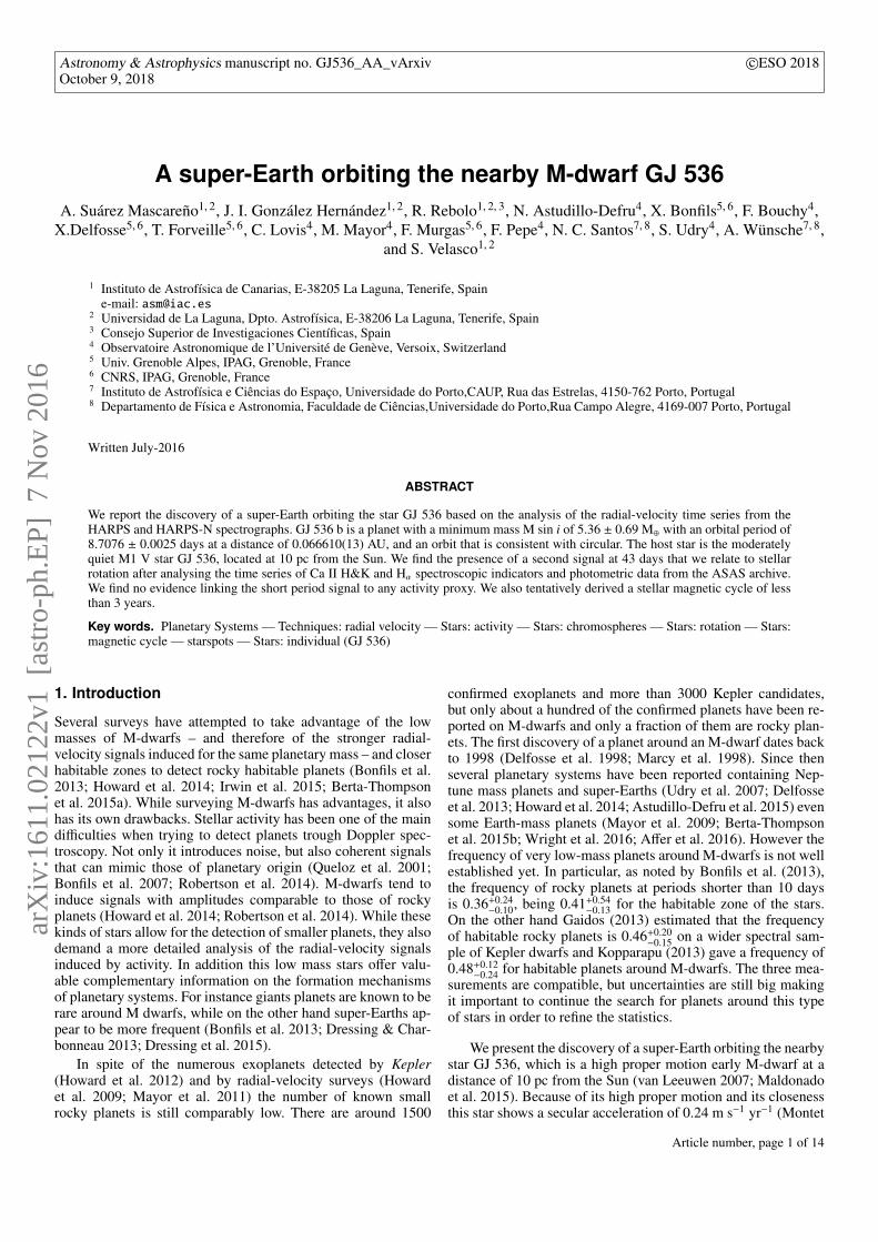
We calculate the Mount Wilson S index and the log10(R′HK) byusing the original Noyes et al. (1984) procedure, following Lo-vis et al. (2011) and Suárez Mascareño et al. (2015). We definetwo triangular-shaped passbands with full width half maximum(FWHM) of 1.09 Å centred at 3968.470 Å and 3933.664 Å forthe Ca II H&K line cores, and for the continuum we use two20 Å wide bands centred at 3901.070 Å (V) and 4001.070 Å(R),as shown in figure 1.

Then the S-index is defined as


A. Suárez Mascareño et al.: A super-Earth orbiting the nearby M-dwarf GJ 536

Fig. 1: Ca II H&K filter of the spectrum of the star GJ536 withthe same shape as the Mount Wilson Ca II H&K passband.

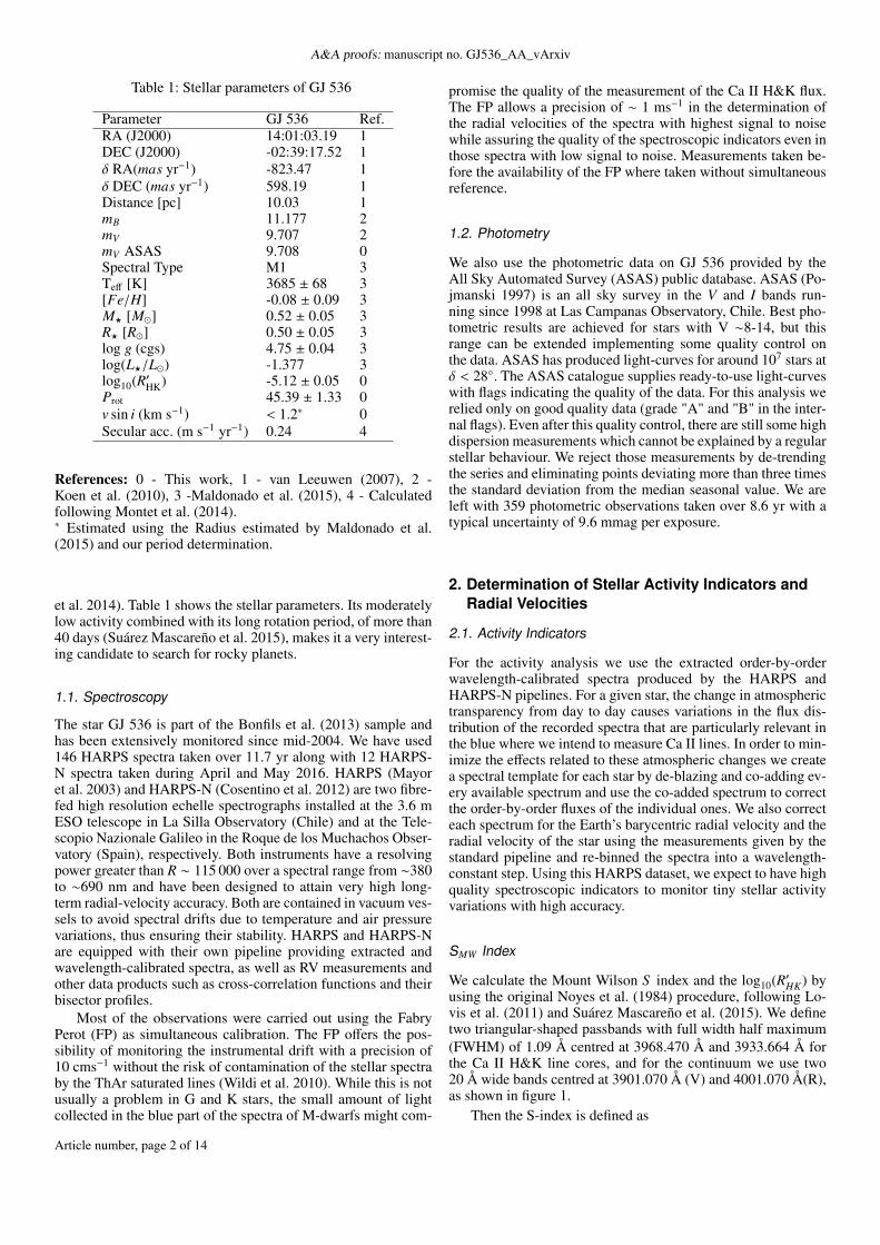
Fig. 2: Spectrum of the M-type star GJ536 showing the Hα filterpassband and continuum bands.

S = αNH + NK

NR + NV+ β, (1)

where NH , NK , NR and NV are the mean fluxes in each passband,while α and β are calibration constants fixed as α = 1.111 andβ = 0.0153 . The S index serves as a measurement of the CaII H&K core flux normalized to the neighbour continuum. Asa normalized index to compare it to other stars we compute thelog10(R′HK) following Suárez Mascareño et al. (2015).

Hα Index

We also use the Hα index, with a simpler passband followingGomes da Silva et al. (2011). It consists of a rectangular band-pass with a width of 1.6 Å and centred at 6562.808 Å (core),and two continuum bands of 10.75 Å and a 8.75 Å wide cen-tred at 6550.87 Å (L) and 6580.31 Å (R), respectively, as seen inFigure 2.

Thus, the Hα index is defined as

HαIndex =Hαcore

HαL + HαR. (2)

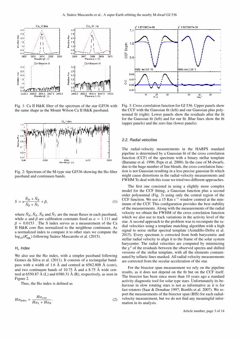
Fig. 3: Cross correlation function for GJ 536. Upper panels showthe CCF with the Gaussian fit (left) and our Gaussian plus poly-nomial fit (right). Lower panels show the residuals after the fitfor the Gaussian fit (left) and for our fit. Blue lines show the fit(upper panels) and the zero line (lower panels).

2.2. Radial velocities

The radial-velocity measurements in the HARPS standardpipeline is determined by a Gaussian fit of the cross correlationfunction (CCF) of the spectrum with a binary stellar template(Baranne et al. 1996; Pepe et al. 2000). In the case of M-dwarfs,due to the huge number of line blends, the cross correlation func-tion is not Gaussian resulting in a less precise gaussian fit whichmight cause distortions in the radial-velocity measurements andFWHM To deal with this issue we tried two different approaches.

The first one consisted in using a slightly more complexmodel for the CCF fitting, a Gaussian function plus a secondorder polynomial (Fig. 3) using only the central region of theCCF function. We use a 15 Km s−1 window centred at the min-imum of the CCF. This configuration provides the best stabilityof the measurements. Along with the measurements of the radialvelocity we obtain the FWHM of the cross correlation functionwhich we also use to track variations in the activity level of thestar. A second approach to the problem was to recompute the ra-dial velocities using a template matching algorithm with a highsignal to noise stellar spectral template (Astudillo-Defru et al.2015). Every spectrum is corrected from both barycentric andstellar radial velocity to align it to the frame of the solar systembarycenter. The radial velocities are computed by minimizingthe χ2 of the residuals between the observed spectra and shiftedversions of the stellar template, with all the elements contami-nated by telluric lines masked. All radial-velocity measurementsare corrected from the secular acceleration of the star.

For the bisector span measurement we rely on the pipelineresults, as it does not depend on the fit but on the CCF itself.The bisector has been since more than 10 years ago a standardactivity diagnostic tool for solar type stars. Unfortunately its be-haviour in slow rotating stars is not as informative as it is forfast rotators (Saar & Donahue 1997; Bonfils et al. 2007). We re-port the measurements of the bisector span (BIS) for each radial-velocity measurement, but we do not find any meaningful infor-mation in its analysis.



2.3. Quality Control of the Data

As the sampling rate of our data is not well suited for modellingfast events, such as flares, and their effect in the radial velocity isnot well understood, we identify and reject points likely affectedby flares by searching for an abnormal behaviour of the activ-ity indicators (Reiners 2009). The process rejected 6 spectra thatcorrespond to flare events of the star with obvious activity en-hancement and line distortion. That leaves us with 140 HARPSspectroscopic observations taken over 10.7 years, with most ofthe measurements taking place after 2013, with a typical expo-sure of 900 s and an average signal to noise ratio of 56 at 5500 Å.We do not apply the quality control procedure to the HARPS-Ndata as the number of spectra is not big enough.

3. Stellar Activity Analysis

In order to properly understand the behaviour of the star, ourfirst step is to analyse the different modulations present in thephotometric and spectroscopic time-series.

We search for periodic variability compatible with both stel-lar rotation and long-term magnetic cycles. We compute thepower spectrum using a Generalised Lomb Scargle Periodogram(Zechmeister & Kürster 2009) and if there is any significant pe-riodicity we fit the detected period using sinusoidal model, or adouble harmonic sinusoidal model to account for the asymmetryof some signals (Berdyugina & Järvinen 2005), with the MPFITroutine (Markwardt 2009).

The significance of the periodogram peak is evaluated usingboth the Cumming (2004) modification of the Horne & Baliu-nas (1986) formula to obtain the spectral density thresholds fora desired false alarm probability (FAP) levels and bootstrap ran-domization (Endl et al. 2001) of the data.

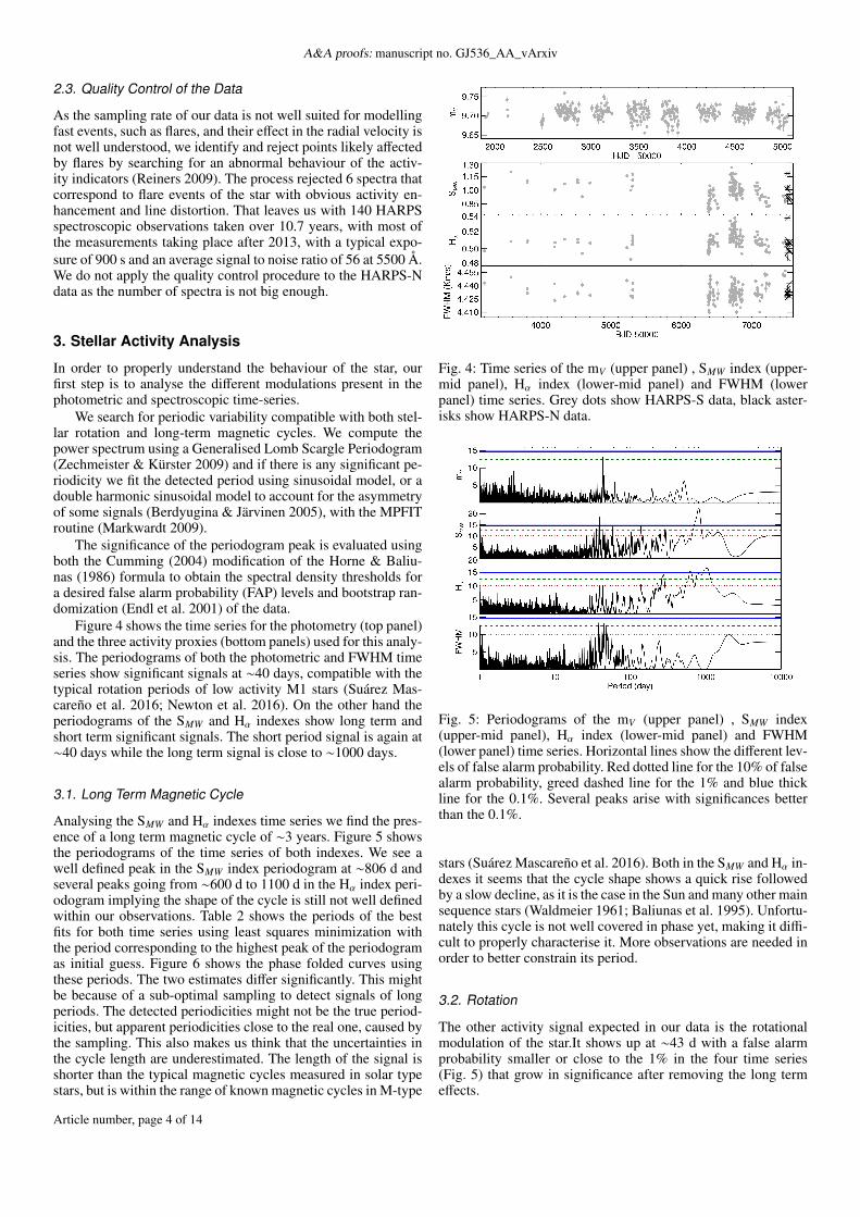
Figure 4 shows the time series for the photometry (top panel)and the three activity proxies (bottom panels) used for this analy-sis. The periodograms of both the photometric and FWHM timeseries show significant signals at ∼40 days, compatible with thetypical rotation periods of low activity M1 stars (Suárez Mas-careño et al. 2016; Newton et al. 2016). On the other hand theperiodograms of the SMW and Hα indexes show long term andshort term significant signals. The short period signal is again at∼40 days while the long term signal is close to ∼1000 days.

3.1. Long Term Magnetic Cycle

Analysing the SMW and Hα indexes time series we find the pres-ence of a long term magnetic cycle of ∼3 years. Figure 5 showsthe periodograms of the time series of both indexes. We see awell defined peak in the SMW index periodogram at ∼806 d andseveral peaks going from ∼600 d to 1100 d in the Hα index peri-odogram implying the shape of the cycle is still not well definedwithin our observations. Table 2 shows the periods of the bestfits for both time series using least squares minimization withthe period corresponding to the highest peak of the periodogramas initial guess. Figure 6 shows the phase folded curves usingthese periods. The two estimates differ significantly. This mightbe because of a sub-optimal sampling to detect signals of longperiods. The detected periodicities might not be the true period-icities, but apparent periodicities close to the real one, caused bythe sampling. This also makes us think that the uncertainties inthe cycle length are underestimated. The length of the signal isshorter than the typical magnetic cycles measured in solar typestars, but is within the range of known magnetic cycles in M-type

Fig. 4: Time series of the mV (upper panel) , SMW index (upper-mid panel), Hα index (lower-mid panel) and FWHM (lowerpanel) time series. Grey dots show HARPS-S data, black aster-isks show HARPS-N data.

Fig. 5: Periodograms of the mV (upper panel) , SMW index(upper-mid panel), Hα index (lower-mid panel) and FWHM(lower panel) time series. Horizontal lines show the different lev-els of false alarm probability. Red dotted line for the 10% of falsealarm probability, greed dashed line for the 1% and blue thickline for the 0.1%. Several peaks arise with significances betterthan the 0.1%.

stars (Suárez Mascareño et al. 2016). Both in the SMW and Hα in-dexes it seems that the cycle shape shows a quick rise followedby a slow decline, as it is the case in the Sun and many other mainsequence stars (Waldmeier 1961; Baliunas et al. 1995). Unfortu-nately this cycle is not well covered in phase yet, making it diffi-cult to properly characterise it. More observations are needed inorder to better constrain its period.

3.2. Rotation

The other activity signal expected in our data is the rotationalmodulation of the star.It shows up at ∼43 d with a false alarmprobability smaller or close to the 1% in the four time series(Fig. 5) that grow in significance after removing the long termeffects.



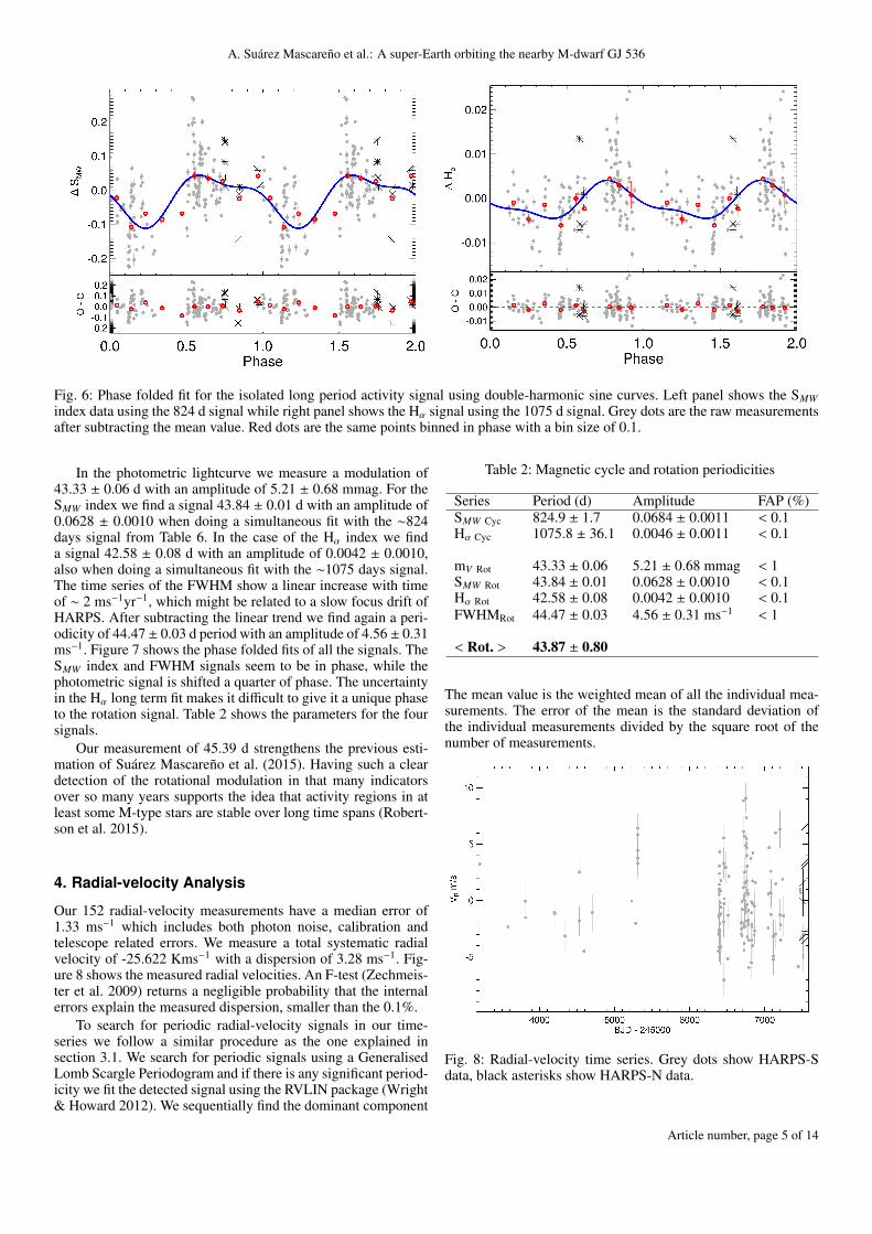
Fig. 6: Phase folded fit for the isolated long period activity signal using double-harmonic sine curves. Left panel shows the SMWindex data using the 824 d signal while right panel shows the Hα signal using the 1075 d signal. Grey dots are the raw measurementsafter subtracting the mean value. Red dots are the same points binned in phase with a bin size of 0.1.

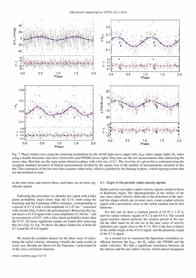
In the photometric lightcurve we measure a modulation of43.33 ± 0.06 d with an amplitude of 5.21 ± 0.68 mmag. For theSMW index we find a signal 43.84 ± 0.01 d with an amplitude of0.0628 ± 0.0010 when doing a simultaneous fit with the ∼824days signal from Table 6. In the case of the Hα index we finda signal 42.58 ± 0.08 d with an amplitude of 0.0042 ± 0.0010,also when doing a simultaneous fit with the ∼1075 days signal.The time series of the FWHM show a linear increase with timeof ∼ 2 ms−1yr−1, which might be related to a slow focus drift ofHARPS. After subtracting the linear trend we find again a peri-odicity of 44.47 ± 0.03 d period with an amplitude of 4.56 ± 0.31ms−1. Figure 7 shows the phase folded fits of all the signals. TheSMW index and FWHM signals seem to be in phase, while thephotometric signal is shifted a quarter of phase. The uncertaintyin the Hα long term fit makes it difficult to give it a unique phaseto the rotation signal. Table 2 shows the parameters for the foursignals.

Our measurement of 45.39 d strengthens the previous esti-mation of Suárez Mascareño et al. (2015). Having such a cleardetection of the rotational modulation in that many indicatorsover so many years supports the idea that activity regions in atleast some M-type stars are stable over long time spans (Robert-son et al. 2015).

4. Radial-velocity Analysis

Our 152 radial-velocity measurements have a median error of1.33 ms−1 which includes both photon noise, calibration andtelescope related errors. We measure a total systematic radialvelocity of -25.622 Kms−1 with a dispersion of 3.28 ms−1. Fig-ure 8 shows the measured radial velocities. An F-test (Zechmeis-ter et al. 2009) returns a negligible probability that the internalerrors explain the measured dispersion, smaller than the 0.1%.

To search for periodic radial-velocity signals in our time-series we follow a similar procedure as the one explained insection 3.1. We search for periodic signals using a GeneralisedLomb Scargle Periodogram and if there is any significant period-icity we fit the detected signal using the RVLIN package (Wright& Howard 2012). We sequentially find the dominant component

Table 2: Magnetic cycle and rotation periodicities

Series Period (d) Amplitude FAP (%)SMW Cyc 824.9 ± 1.7 0.0684 ± 0.0011 < 0.1Hα Cyc 1075.8 ± 36.1 0.0046 ± 0.0011 < 0.1

mV Rot 43.33 ± 0.06 5.21 ± 0.68 mmag < 1SMW Rot 43.84 ± 0.01 0.0628 ± 0.0010 < 0.1Hα Rot 42.58 ± 0.08 0.0042 ± 0.0010 < 0.1FWHMRot 44.47 ± 0.03 4.56 ± 0.31 ms−1 < 1

< Rot. > 43.87 ± 0.80

The mean value is the weighted mean of all the individual mea-surements. The error of the mean is the standard deviation ofthe individual measurements divided by the square root of thenumber of measurements.

Fig. 8: Radial-velocity time series. Grey dots show HARPS-Sdata, black asterisks show HARPS-N data.



Fig. 7: Phase folded curve using the rotational modulation for the ASAS light curve (upper left), SMW index (upper right), Hα indexusing a double-harmonic sine curve (lower left) and FWHM (lower right). Grey dots are the raw measurements after subtracting themean value. Red dots are the same points binned in phase with a bin size of 0.1. The error bar of a given bin is estimated using theweighted standard deviation of binned measurements divided by the square root of the number of measurements included in thisbin. This estimation of the bin error bars assumes white noise, which is justified by the binning in phase, which regroups points thatare uncorrelated in time.

in the time series and remove them, until there are no more sig-nificant signals.

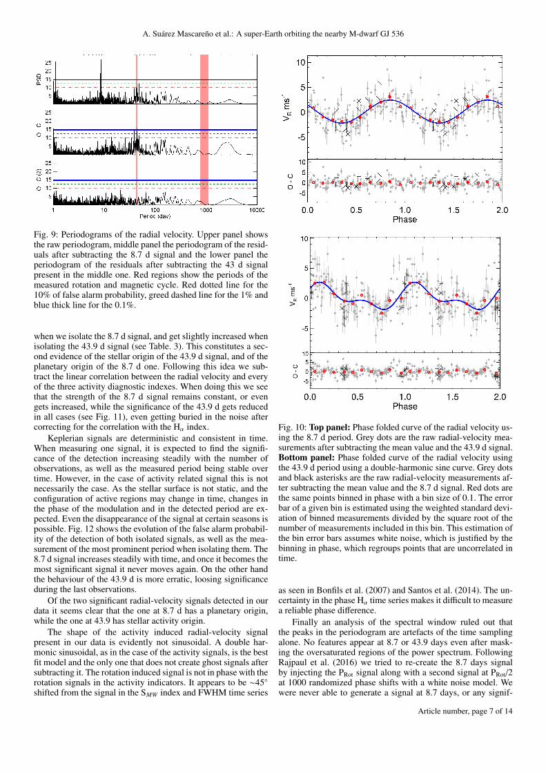
Following this procedure we identify one signal with a falsealarm probability much better than the 0.1%, both using thebootstrap and the Cumming (2004) estimates, corresponding toa period of 8.7 d with a semi-amplitude of 2.47 ms−1 consistentwith circular (Fig. 9 shows the periodogram). Removing this sig-nal leaves a 43.9 d signal with a semi amplitude of 2.86 ms−1 andan eccentricity of 0.57, with a false alarm probability better thanthe 0.1%. No more significant signals are found after removingthis two (Fig. 9). Fig. 10 shows the phase folded fits of both the8.7 d and the 43.9 d signals.

We tested the available dataset for the three ways of calcu-lating the radial velocity, obtaining virtually the same results inevery case. Results are shown for the Gaussian + polynomial fitof the cross correlation function.

4.1. Origin of the periodic radial-velocity signals

Stellar activity can induce radial-velocity signals similar to thoseof Keplerian origin. The inhomogeneities in the surface of thestar cause radial-velocity shifts due to the distortion of the spec-tral line shapes which can, in some cases, create a radial-velocitysignal with a periodicity close to the stellar rotation and its firstharmonic.

For this star we have a rotation period of 45.39 ± 1.33 d,and two radial-velocity signals of 8.7 d and 43.9 d. The secondsignal matches almost perfectly the rotation period of the star.On the other hand we do not see in the time series of activityindicators any signal close to the 8.7 d. This is the first evidenceof the stellar origin of the 43.9 d signal, and the planetary originof the 8.7 d signal.

As a second test we measured the Spearman correlation co-efficient between the SMW , the Hα index, the FWHM and theradial velocities. We find a significant correlation between allthe indexes and the raw radial velocity, which almost disappears



Fig. 9: Periodograms of the radial velocity. Upper panel showsthe raw periodogram, middle panel the periodogram of the resid-uals after subtracting the 8.7 d signal and the lower panel theperiodogram of the residuals after subtracting the 43 d signalpresent in the middle one. Red regions show the periods of themeasured rotation and magnetic cycle. Red dotted line for the10% of false alarm probability, greed dashed line for the 1% andblue thick line for the 0.1%.

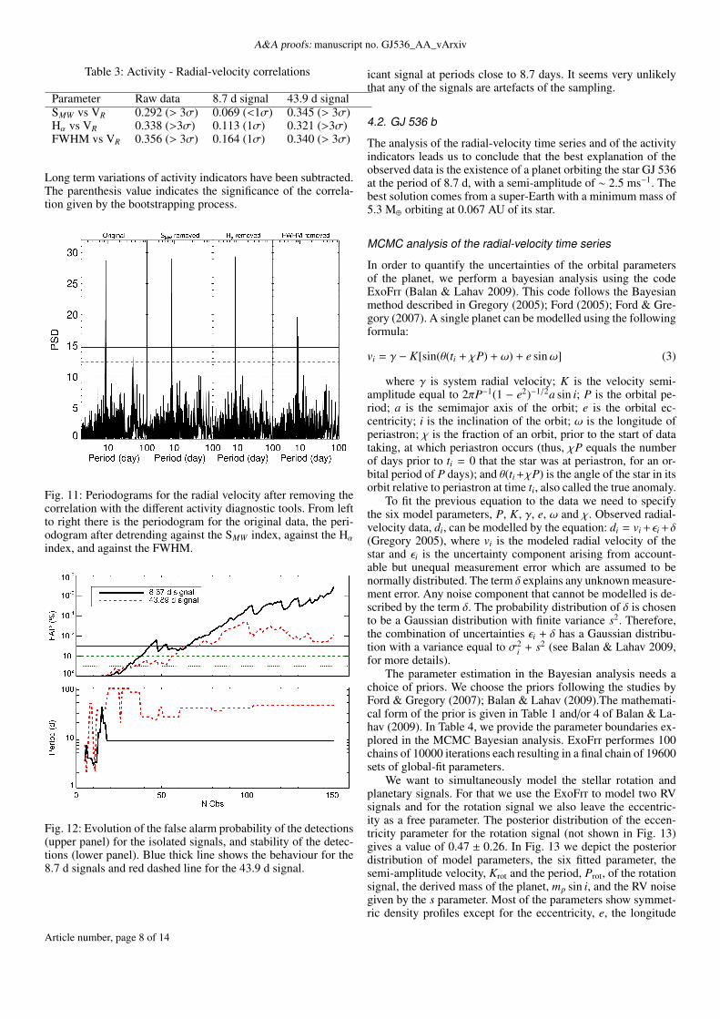
when we isolate the 8.7 d signal, and get slightly increased whenisolating the 43.9 d signal (see Table. 3). This constitutes a sec-ond evidence of the stellar origin of the 43.9 d signal, and of theplanetary origin of the 8.7 d one. Following this idea we sub-tract the linear correlation between the radial velocity and everyof the three activity diagnostic indexes. When doing this we seethat the strength of the 8.7 d signal remains constant, or evengets increased, while the significance of the 43.9 d gets reducedin all cases (see Fig. 11), even getting buried in the noise aftercorrecting for the correlation with the Hα index.

Keplerian signals are deterministic and consistent in time.When measuring one signal, it is expected to find the signifi-cance of the detection increasing steadily with the number ofobservations, as well as the measured period being stable overtime. However, in the case of activity related signal this is notnecessarily the case. As the stellar surface is not static, and theconfiguration of active regions may change in time, changes inthe phase of the modulation and in the detected period are ex-pected. Even the disappearance of the signal at certain seasons ispossible. Fig. 12 shows the evolution of the false alarm probabil-ity of the detection of both isolated signals, as well as the mea-surement of the most prominent period when isolating them. The8.7 d signal increases steadily with time, and once it becomes themost significant signal it never moves again. On the other handthe behaviour of the 43.9 d is more erratic, loosing significanceduring the last observations.

Of the two significant radial-velocity signals detected in ourdata it seems clear that the one at 8.7 d has a planetary origin,while the one at 43.9 has stellar activity origin.

The shape of the activity induced radial-velocity signalpresent in our data is evidently not sinusoidal. A double har-monic sinusoidal, as in the case of the activity signals, is the bestfit model and the only one that does not create ghost signals aftersubtracting it. The rotation induced signal is not in phase with therotation signals in the activity indicators. It appears to be ∼45◦shifted from the signal in the SMW index and FWHM time series

Fig. 10: Top panel: Phase folded curve of the radial velocity us-ing the 8.7 d period. Grey dots are the raw radial-velocity mea-surements after subtracting the mean value and the 43.9 d signal.Bottom panel: Phase folded curve of the radial velocity usingthe 43.9 d period using a double-harmonic sine curve. Grey dotsand black asterisks are the raw radial-velocity measurements af-ter subtracting the mean value and the 8.7 d signal. Red dots arethe same points binned in phase with a bin size of 0.1. The errorbar of a given bin is estimated using the weighted standard devi-ation of binned measurements divided by the square root of thenumber of measurements included in this bin. This estimation ofthe bin error bars assumes white noise, which is justified by thebinning in phase, which regroups points that are uncorrelated intime.

as seen in Bonfils et al. (2007) and Santos et al. (2014). The un-certainty in the phase Hα time series makes it difficult to measurea reliable phase difference.

Finally an analysis of the spectral window ruled out thatthe peaks in the periodogram are artefacts of the time samplingalone. No features appear at 8.7 or 43.9 days even after mask-ing the oversaturated regions of the power spectrum. FollowingRajpaul et al. (2016) we tried to re-create the 8.7 days signalby injecting the PRot signal along with a second signal at PRot/2at 1000 randomized phase shifts with a white noise model. Wewere never able to generate a signal at 8.7 days, or any signif-



Table 3: Activity - Radial-velocity correlations

Parameter Raw data 8.7 d signal 43.9 d signalSMW vs VR 0.292 (> 3σ) 0.069 (<1σ) 0.345 (> 3σ)Hα vs VR 0.338 (>3σ) 0.113 (1σ) 0.321 (>3σ)FWHM vs VR 0.356 (> 3σ) 0.164 (1σ) 0.340 (> 3σ)

Long term variations of activity indicators have been subtracted.The parenthesis value indicates the significance of the correla-tion given by the bootstrapping process.

Fig. 11: Periodograms for the radial velocity after removing thecorrelation with the different activity diagnostic tools. From leftto right there is the periodogram for the original data, the peri-odogram after detrending against the SMW index, against the Hα

index, and against the FWHM.

Fig. 12: Evolution of the false alarm probability of the detections(upper panel) for the isolated signals, and stability of the detec-tions (lower panel). Blue thick line shows the behaviour for the8.7 d signals and red dashed line for the 43.9 d signal.

icant signal at periods close to 8.7 days. It seems very unlikelythat any of the signals are artefacts of the sampling.

4.2. GJ 536 b

The analysis of the radial-velocity time series and of the activityindicators leads us to conclude that the best explanation of theobserved data is the existence of a planet orbiting the star GJ 536at the period of 8.7 d, with a semi-amplitude of ∼ 2.5 ms−1. Thebest solution comes from a super-Earth with a minimum mass of5.3 M⊕ orbiting at 0.067 AU of its star.

MCMC analysis of the radial-velocity time series

In order to quantify the uncertainties of the orbital parametersof the planet, we perform a bayesian analysis using the codeExoFit (Balan & Lahav 2009). This code follows the Bayesianmethod described in Gregory (2005); Ford (2005); Ford & Gre-gory (2007). A single planet can be modelled using the followingformula:

vi = γ − K[sin(θ(ti + χP) + ω) + e sinω] (3)

where γ is system radial velocity; K is the velocity semi-amplitude equal to 2πP−1(1 − e2)−1/2a sin i; P is the orbital pe-riod; a is the semimajor axis of the orbit; e is the orbital ec-centricity; i is the inclination of the orbit; ω is the longitude ofperiastron; χ is the fraction of an orbit, prior to the start of datataking, at which periastron occurs (thus, χP equals the numberof days prior to ti = 0 that the star was at periastron, for an or-bital period of P days); and θ(ti +χP) is the angle of the star in itsorbit relative to periastron at time ti, also called the true anomaly.

To fit the previous equation to the data we need to specifythe six model parameters, P, K, γ, e, ω and χ. Observed radial-velocity data, di, can be modelled by the equation: di = vi + εi +δ(Gregory 2005), where vi is the modeled radial velocity of thestar and εi is the uncertainty component arising from account-able but unequal measurement error which are assumed to benormally distributed. The term δ explains any unknown measure-ment error. Any noise component that cannot be modelled is de-scribed by the term δ. The probability distribution of δ is chosento be a Gaussian distribution with finite variance s2. Therefore,the combination of uncertainties εi + δ has a Gaussian distribu-tion with a variance equal to σ2

i + s2 (see Balan & Lahav 2009,for more details).

The parameter estimation in the Bayesian analysis needs achoice of priors. We choose the priors following the studies byFord & Gregory (2007); Balan & Lahav (2009).The mathemati-cal form of the prior is given in Table 1 and/or 4 of Balan & La-hav (2009). In Table 4, we provide the parameter boundaries ex-plored in the MCMC Bayesian analysis. ExoFit performes 100chains of 10000 iterations each resulting in a final chain of 19600sets of global-fit parameters.

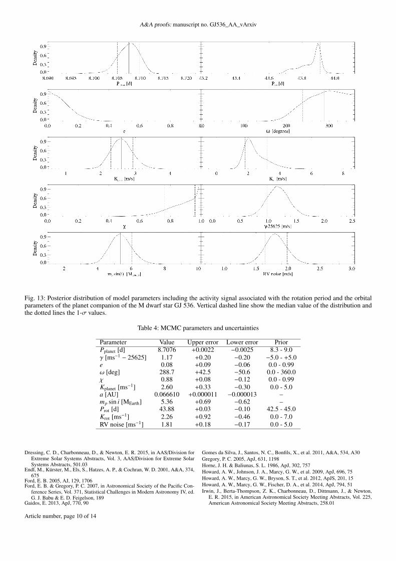
We want to simultaneously model the stellar rotation andplanetary signals. For that we use the ExoFit to model two RVsignals and for the rotation signal we also leave the eccentric-ity as a free parameter. The posterior distribution of the eccen-tricity parameter for the rotation signal (not shown in Fig. 13)gives a value of 0.47 ± 0.26. In Fig. 13 we depict the posteriordistribution of model parameters, the six fitted parameter, thesemi-amplitude velocity, Krot and the period, Prot, of the rotationsignal, the derived mass of the planet, mp sin i, and the RV noisegiven by the s parameter. Most of the parameters show symmet-ric density profiles except for the eccentricity, e, the longitude



of periastron, ω, the fraction χ of the orbit at which the perias-tron occurs. We note that the density profile of the rotation perioddisplays a tail towards slightly lower values although the rotationperiod is well defined.

In Table 4 we show the final parameters and uncertainties ob-tained with the MCMC bayesian analysis with the code ExoFit.

5. Discussion

We detect the presence of a planet with a semi-amplitude of 2.60m s−1 that, given the stellar mass of 0.52 M�, converts to m sini of 5.36 M⊕, orbiting with a period of 8.7 d around GJ 536,an M-type star of 0.52 M� with a rotation period of 43.9 d thatshows an additional activity signal compatible with an activitycycle shorter than 3 yr.

The planet is a small super-Earth with an equilibrium tem-perature 344 K for a Bond albedo A = 0.75 and 487 K for A=0.Following Kasting et al. (1993) and Selsis et al. (2007) we per-form a simple estimation of the habitable zone (HZ) of this star.The HZ would go from 0.2048 to 0.3975 AU in the narrowestcase (cloud free model) and 0.1044 to 0.5470 AU in the broaderone (fully clouded model). This corresponds to orbital periodsfrom 46 to 126 days in the narrower case, and 17 to 204 days inthe broader one.

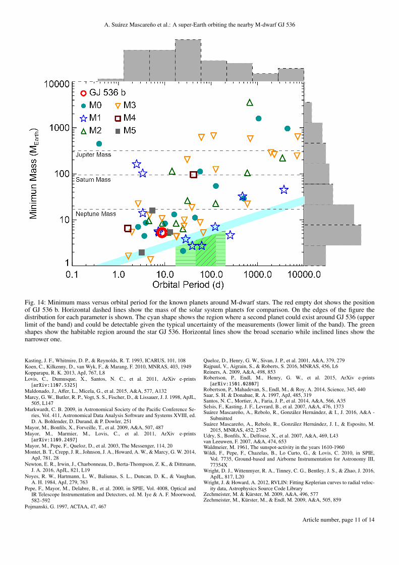
GJ 536 b is in the lower part of the Mass vs Period diagramof known planets around M-dwarf stars (Fig. 14). The planet istoo close to the star to be considered habitable. For this star thehabitable zone would be from ∼20 days to ∼ 40 days.

GJ 536 is a quiet early M-dwarf, with a rotation period onthe upper end of the stars of its kind (Newton et al. 2016; SuárezMascareño et al. 2016). Its rotation induced radial-velocity sig-nal has a semi-amplitude of 2.26 ms−1 and seems to be stableenough to allow for a clean enough periodogram and to be cor-rectly characterized. The phase of the rotation induced signalseems to be advanced ∼45◦ with respect to the signals in SMWindex and FWHM time series. There is a hint for a short ac-tivity cycle shorter than 3 yr, which would put it in the lowerend of the stars of its kind (Suárez Mascareño et al. 2016), andwhose amplitude is so small that would need further follow-upto be properly characterized. The radial-velocity signal inducedby this cycle is at this point beyond our detection capabilities.

Given the rms of the residuals there is still room for the de-tection of more planets in this system, especially at orbital pe-riods longer than the rotation period. Fig. 14 shows the upperlimits to the mass of those hypothetical companions. The stabil-ity of its rotation signals and the low amplitude of the radial-velocity signals with a magnetic origin makes this star a goodcandidate to search for longer period planets of moderate mass.A rough estimate of the detection limits tells us there is still roomfor Earth-like planets (∼ 1 M⊕) at orbits smaller than 10, super-Earths (< 10 M⊕) at orbits going from 10 to 400 days, and evenfor a Neptune mass planet (< 20 M⊕) at periods longer than ∼3yr. Giant planets on the other hand are discarded except for ex-tremely long orbital periods. The time-span of the observationsand the RMS of the residuals completely discards the presenceof any planet bigger than twice the mass of Neptune with an or-bital period shorter than ∼ 20 years.

6. Conclusions

We have analysed 152 high resolution spectra and 359 photomet-ric observations to study the presence of planetary companions

around the M-dwarf star GJ 536 and its stellar activity. We de-tected two significant radial-velocity signals, at periods of 8.7and 43.8 days, respectively.

From the available photometric and spectroscopic informa-tion we conclude that the 8.7 d signal is caused by a 5.3 M⊕planet with semi major axis of 0.067 AU and equilibrium tem-perature lower than 500K. The short period of the planet makesit a potential transiting candidate. Detecting the transits wouldgive a new constraining point to the mass-radius diagram.

The second radial-velocity signal of period 43.8 d and semiamplitude of 1.6 ms−1 is a magnetic activity induced signal re-lated to the rotation of the star. We also found a magnetic cycleshorter than 3 yr which would place this star among those withthe shortest reported magnetic cycles.

We have studied and set limits to the presence of other plan-etary companions taking into account the rms of the residualsafter fitting both the planet and the rotation induced signal. Thesystem still has room for other low mass companions, but plan-ets more massive than Neptune are discarded except at extremelylong orbital periods, beyond the habitable zone of the star.

Acknowledgements

This work has been financed by the Spanish Ministry projectMINECO AYA2014-56359-P . J.I.G.H. acknowledges financialsupport from the Spanish MINECO under the 2013 Ramón yCajal program MINECO RYC-2013-14875. X.B., X.D., T.F.and F.M. acknowledge the support of the French Agence Na-tionale de la Recherche (ANR), under the program ANR-12-BS05- 0012 Exo-atmos. X.B. and A.W. acknowledge fund-ing from the European Research Council under the ERCGrant Agreement No. 337591-ExTrA. This work was sup-ported by Fundação para a Ciência e a Tecnologia (FCT)within projects reference PTDC/FIS-AST/1526/2014 (POCI-01-0145-FEDER-016886) and UID/FIS/04434/2013 (POCI-01-0145-FEDER-007672). NCS acknowledge support by throughInvestigador FCT contract of reference IF/00169/2012, andPOPH/FSE (EC) by FEDER funding through the program “Pro-grama Operacional de Factores de Competitividade - COM-PETE”. This work is based on data obtained HARPS publicdatabase at the European Southern Observatory (ESO). This re-search has made extensive use of the SIMBAD database, op-erated at CDS, Strasbourg, France and NASA’s AstrophysicsData System. We are grateful to all the observers of the follow-ing ESO projects, whose data we are using: 072.C-0488, 085.C-0019, 183.C-0972 and 191.C-087.

ReferencesAffer, L., Micela, G., Damasso, M., et al. 2016, A&A, 593, A117Astudillo-Defru, N., Bonfils, X., Delfosse, X., et al. 2015, A&A, 575, A119Balan, S. T. & Lahav, O. 2009, MNRAS, 394, 1936Baliunas, S. L., Donahue, R. A., Soon, W. H., et al. 1995, ApJ, 438, 269Baranne, A., Queloz, D., Mayor, M., et al. 1996, A&AS, 119, 373Berdyugina, S. V. & Järvinen, S. P. 2005, Astronomische Nachrichten, 326, 283Berta-Thompson, Z. K., Irwin, J., Charbonneau, D., et al. 2015a, Nature, 527,

204Berta-Thompson, Z. K., Irwin, J., Charbonneau, D., et al. 2015b, NAT, 527, 204Bonfils, X., Delfosse, X., Udry, S., et al. 2013, A&A, 549, A109Bonfils, X., Mayor, M., Delfosse, X., et al. 2007, A&A, 474, 293Cosentino, R., Lovis, C., Pepe, F., et al. 2012, in SPIE, Vol. 8446, Ground-based

and Airborne Instrumentation for Astronomy IV, 84461VCumming, A. 2004, MNRAS, 354, 1165Delfosse, X., Bonfils, X., Forveille, T., et al. 2013, A&A, 553, A8Delfosse, X., Forveille, T., Perrier, C., & Mayor, M. 1998, A&A, 331, 581Dressing, C. D. & Charbonneau, D. 2013, ApJ, 767, 95



Fig. 13: Posterior distribution of model parameters including the activity signal associated with the rotation period and the orbitalparameters of the planet companion of the M dwarf star GJ 536. Vertical dashed line show the median value of the distribution andthe dotted lines the 1-σ values.

Table 4: MCMC parameters and uncertainties

Parameter Value Upper error Lower error PriorPplanet [d] 8.7076 +0.0022 −0.0025 8.3 - 9.0γ [ms−1 − 25625] 1.17 +0.20 −0.20 −5.0 - +5.0e 0.08 +0.09 −0.06 0.0 - 0.99ω [deg] 288.7 +42.5 −50.6 0.0 - 360.0χ 0.88 +0.08 −0.12 0.0 - 0.99Kplanet [ms−1] 2.60 +0.33 −0.30 0.0 - 5.0a [AU] 0.066610 +0.000011 −0.000013 –mp sin i [MEarth] 5.36 +0.69 −0.62 –Prot [d] 43.88 +0.03 −0.10 42.5 - 45.0Krot [ms−1] 2.26 +0.92 −0.46 0.0 - 7.0RV noise [ms−1] 1.81 +0.18 −0.17 0.0 - 5.0

Dressing, C. D., Charbonneau, D., & Newton, E. R. 2015, in AAS/Division forExtreme Solar Systems Abstracts, Vol. 3, AAS/Division for Extreme SolarSystems Abstracts, 501.03

Endl, M., Kürster, M., Els, S., Hatzes, A. P., & Cochran, W. D. 2001, A&A, 374,675

Ford, E. B. 2005, AJ, 129, 1706Ford, E. B. & Gregory, P. C. 2007, in Astronomical Society of the Pacific Con-

ference Series, Vol. 371, Statistical Challenges in Modern Astronomy IV, ed.G. J. Babu & E. D. Feigelson, 189

Gaidos, E. 2013, ApJ, 770, 90

Gomes da Silva, J., Santos, N. C., Bonfils, X., et al. 2011, A&A, 534, A30Gregory, P. C. 2005, ApJ, 631, 1198Horne, J. H. & Baliunas, S. L. 1986, ApJ, 302, 757Howard, A. W., Johnson, J. A., Marcy, G. W., et al. 2009, ApJ, 696, 75Howard, A. W., Marcy, G. W., Bryson, S. T., et al. 2012, ApJS, 201, 15Howard, A. W., Marcy, G. W., Fischer, D. A., et al. 2014, ApJ, 794, 51Irwin, J., Berta-Thompson, Z. K., Charbonneau, D., Dittmann, J., & Newton,

E. R. 2015, in American Astronomical Society Meeting Abstracts, Vol. 225,American Astronomical Society Meeting Abstracts, 258.01



Fig. 14: Minimum mass versus orbital period for the known planets around M-dwarf stars. The red empty dot shows the positionof GJ 536 b. Horizontal dashed lines show the mass of the solar system planets for comparison. On the edges of the figure thedistribution for each parameter is shown. The cyan shape shows the region where a second planet could exist around GJ 536 (upperlimit of the band) and could be detectable given the typical uncertainty of the measurements (lower limit of the band). The greenshapes show the habitable region around the star GJ 536. Horizontal lines show the broad scenario while inclined lines show thenarrower one.

Kasting, J. F., Whitmire, D. P., & Reynolds, R. T. 1993, ICARUS, 101, 108Koen, C., Kilkenny, D., van Wyk, F., & Marang, F. 2010, MNRAS, 403, 1949Kopparapu, R. K. 2013, ApJ, 767, L8Lovis, C., Dumusque, X., Santos, N. C., et al. 2011, ArXiv e-prints

[arXiv:1107.5325]Maldonado, J., Affer, L., Micela, G., et al. 2015, A&A, 577, A132Marcy, G. W., Butler, R. P., Vogt, S. S., Fischer, D., & Lissauer, J. J. 1998, ApJL,

505, L147Markwardt, C. B. 2009, in Astronomical Society of the Pacific Conference Se-

ries, Vol. 411, Astronomical Data Analysis Software and Systems XVIII, ed.D. A. Bohlender, D. Durand, & P. Dowler, 251

Mayor, M., Bonfils, X., Forveille, T., et al. 2009, A&A, 507, 487Mayor, M., Marmier, M., Lovis, C., et al. 2011, ArXiv e-prints

[arXiv:1109.2497]Mayor, M., Pepe, F., Queloz, D., et al. 2003, The Messenger, 114, 20Montet, B. T., Crepp, J. R., Johnson, J. A., Howard, A. W., & Marcy, G. W. 2014,

ApJ, 781, 28Newton, E. R., Irwin, J., Charbonneau, D., Berta-Thompson, Z. K., & Dittmann,

J. A. 2016, ApJL, 821, L19Noyes, R. W., Hartmann, L. W., Baliunas, S. L., Duncan, D. K., & Vaughan,

A. H. 1984, ApJ, 279, 763Pepe, F., Mayor, M., Delabre, B., et al. 2000, in SPIE, Vol. 4008, Optical and

IR Telescope Instrumentation and Detectors, ed. M. Iye & A. F. Moorwood,582–592

Pojmanski, G. 1997, ACTAA, 47, 467

Queloz, D., Henry, G. W., Sivan, J. P., et al. 2001, A&A, 379, 279Rajpaul, V., Aigrain, S., & Roberts, S. 2016, MNRAS, 456, L6Reiners, A. 2009, A&A, 498, 853Robertson, P., Endl, M., Henry, G. W., et al. 2015, ArXiv e-prints

[arXiv:1501.02807]Robertson, P., Mahadevan, S., Endl, M., & Roy, A. 2014, Science, 345, 440Saar, S. H. & Donahue, R. A. 1997, ApJ, 485, 319Santos, N. C., Mortier, A., Faria, J. P., et al. 2014, A&A, 566, A35Selsis, F., Kasting, J. F., Levrard, B., et al. 2007, A&A, 476, 1373Suárez Mascareño, A., Rebolo, R., González Hernández, & I., J. 2016, A&A -

SubmittedSuárez Mascareño, A., Rebolo, R., González Hernández, J. I., & Esposito, M.

2015, MNRAS, 452, 2745Udry, S., Bonfils, X., Delfosse, X., et al. 2007, A&A, 469, L43van Leeuwen, F. 2007, A&A, 474, 653Waldmeier, M. 1961, The sunspot-activity in the years 1610-1960Wildi, F., Pepe, F., Chazelas, B., Lo Curto, G., & Lovis, C. 2010, in SPIE,

Vol. 7735, Ground-based and Airborne Instrumentation for Astronomy III,77354X

Wright, D. J., Wittenmyer, R. A., Tinney, C. G., Bentley, J. S., & Zhao, J. 2016,ApJL, 817, L20

Wright, J. & Howard, A. 2012, RVLIN: Fitting Keplerian curves to radial veloc-ity data, Astrophysics Source Code Library

Zechmeister, M. & Kürster, M. 2009, A&A, 496, 577Zechmeister, M., Kürster, M., & Endl, M. 2009, A&A, 505, 859



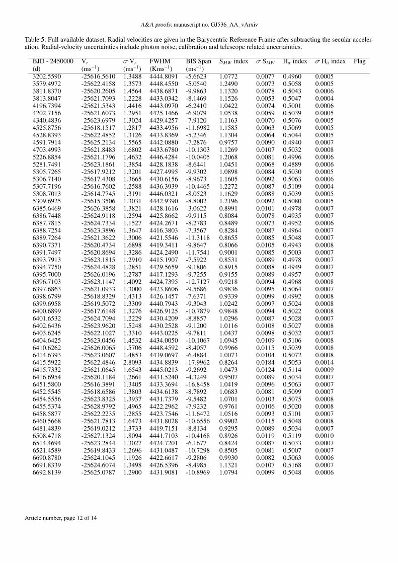
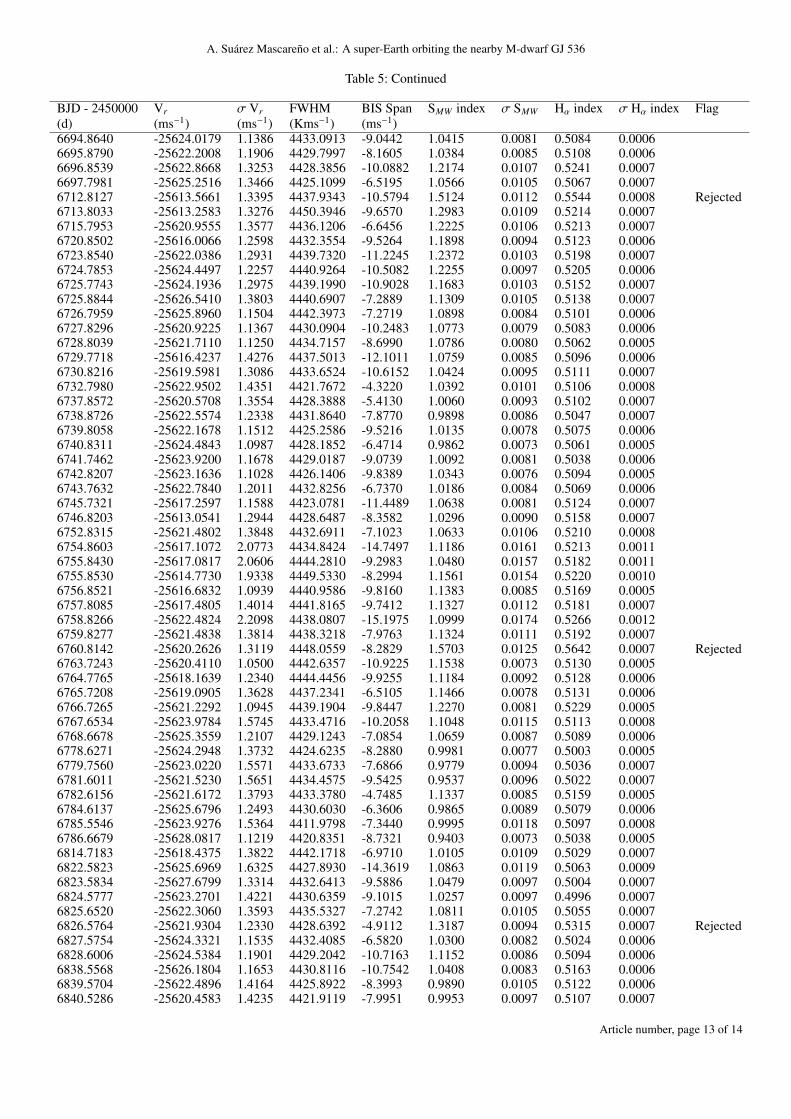
Table 5: Full available dataset. Radial velocities are given in the Barycentric Reference Frame after subtracting the secular acceler-ation. Radial-velocity uncertainties include photon noise, calibration and telescope related uncertainties.

BJD - 2450000 Vr σ Vr FWHM BIS Span SMW index σ SMW Hα index σ Hα index Flag(d) (ms−1) (ms−1) (Kms−1) (ms−1)3202.5590 -25616.5610 1.3488 4444.8091 -5.6623 1.0772 0.0077 0.4960 0.00053579.4972 -25622.4158 1.3573 4448.4550 -5.0540 1.2490 0.0073 0.5058 0.00053811.8370 -25620.2605 1.4564 4438.6871 -9.9863 1.1320 0.0078 0.5043 0.00063813.8047 -25621.7093 1.2228 4433.0342 -8.1469 1.1526 0.0053 0.5047 0.00044196.7394 -25621.5343 1.4416 4443.0970 -6.2410 1.0422 0.0074 0.5001 0.00064202.7156 -25621.6073 1.2951 4425.1466 -6.9079 1.0538 0.0059 0.5039 0.00054340.4836 -25623.6979 1.3024 4429.4257 -7.9120 1.1163 0.0070 0.5076 0.00054525.8756 -25618.1517 1.2817 4433.4956 -11.6982 1.1585 0.0063 0.5069 0.00054528.8393 -25622.4852 1.3126 4433.8369 -5.2346 1.1304 0.0064 0.5044 0.00054591.7914 -25625.2134 1.5565 4442.0880 -7.2876 0.9757 0.0090 0.4940 0.00074703.4993 -25621.8483 1.6802 4433.6780 -10.1303 1.1269 0.0107 0.5032 0.00085226.8854 -25621.1796 1.4632 4446.4284 -10.0405 1.2068 0.0081 0.4996 0.00065281.7491 -25623.1861 1.3854 4428.1838 -8.6441 1.0451 0.0068 0.4889 0.00065305.7265 -25617.9212 1.3201 4427.4995 -9.9302 1.0898 0.0084 0.5030 0.00055306.7140 -25617.4308 1.3665 4430.6156 -8.9673 1.1605 0.0092 0.5063 0.00065307.7196 -25616.7602 1.2588 4436.3939 -10.4465 1.2272 0.0087 0.5109 0.00045308.7013 -25614.7745 1.3191 4446.0321 -8.0523 1.1629 0.0088 0.5039 0.00055309.6925 -25615.3506 1.3031 4442.9390 -8.8002 1.2196 0.0092 0.5080 0.00056385.6469 -25626.3858 1.3821 4428.1616 -3.0622 0.8991 0.0101 0.4978 0.00076386.7448 -25624.9118 1.2594 4425.8662 -9.9115 0.8084 0.0078 0.4935 0.00076387.7815 -25624.7334 1.1527 4424.2671 -8.2783 0.8489 0.0073 0.4952 0.00066388.7254 -25623.3896 1.3647 4416.3803 -7.3567 0.8284 0.0087 0.4964 0.00076389.7264 -25621.3622 1.3006 4421.5546 -11.3118 0.8655 0.0085 0.5048 0.00076390.7371 -25620.4734 1.6898 4419.3411 -9.8647 0.8066 0.0105 0.4943 0.00086391.7497 -25620.8694 1.3286 4424.2490 -11.7541 0.9001 0.0085 0.5003 0.00076393.7913 -25623.1815 1.2910 4415.1907 -7.5922 0.8531 0.0089 0.4978 0.00076394.7750 -25624.4828 1.2851 4429.5659 -9.1806 0.8915 0.0088 0.4949 0.00076395.7000 -25626.0196 1.2787 4417.1293 -9.7255 0.9155 0.0089 0.4957 0.00076396.7103 -25623.1147 1.4092 4424.7395 -12.7127 0.9218 0.0094 0.4968 0.00086397.6863 -25621.0933 1.3000 4423.8606 -9.5686 0.9836 0.0095 0.5064 0.00076398.6799 -25618.8329 1.4313 4426.1457 -7.6371 0.9339 0.0099 0.4992 0.00086399.6958 -25619.5072 1.3309 4440.7943 -9.3043 1.0242 0.0097 0.5024 0.00086400.6899 -25617.6148 1.3276 4426.9125 -10.7879 0.9848 0.0094 0.5022 0.00086401.6532 -25624.7094 1.2229 4430.4209 -8.8857 1.0296 0.0087 0.5028 0.00076402.6436 -25623.9620 1.5248 4430.2528 -9.1200 1.0116 0.0108 0.5027 0.00086403.6245 -25622.1027 1.3310 4443.0225 -9.7811 1.0437 0.0098 0.5032 0.00076404.6425 -25623.0456 1.4532 4434.0050 -10.1067 1.0945 0.0109 0.5106 0.00086410.6262 -25626.0065 1.5706 4448.4592 -8.4057 0.9966 0.0115 0.5039 0.00086414.6393 -25623.0607 1.4853 4439.0697 -6.4884 1.0073 0.0104 0.5072 0.00086415.5922 -25622.4846 2.8093 4434.8839 -17.9962 0.8264 0.0184 0.5053 0.00146415.7332 -25621.0645 1.6543 4445.0213 -9.2692 1.0473 0.0124 0.5114 0.00096416.6954 -25620.1184 1.2661 4431.5240 -4.3249 0.9507 0.0089 0.5034 0.00076451.5800 -25616.3891 1.3405 4433.3694 -16.8458 1.0419 0.0096 0.5063 0.00076452.5545 -25618.6586 1.3803 4434.6138 -8.7892 1.0683 0.0081 0.5099 0.00076454.5556 -25623.8325 1.3937 4431.7379 -9.5482 1.0701 0.0103 0.5075 0.00086455.5374 -25628.9792 1.4965 4422.2962 -7.9232 0.9761 0.0106 0.5020 0.00086458.5877 -25622.2235 1.2855 4423.7546 -11.6472 1.0516 0.0093 0.5101 0.00076460.5668 -25621.7813 1.6473 4431.8028 -10.6556 0.9902 0.0115 0.5048 0.00086481.4839 -25619.0212 1.3733 4419.7151 -8.8134 0.9295 0.0089 0.5034 0.00076508.4718 -25627.1324 1.8094 4441.7103 -10.4168 0.8926 0.0119 0.5119 0.00106514.4694 -25623.2844 1.3027 4424.7201 -6.1677 0.8424 0.0087 0.5033 0.00076521.4589 -25619.8433 1.2696 4431.0487 -10.7298 0.8505 0.0081 0.5007 0.00076690.8780 -25624.1045 1.1926 4422.6617 -9.2806 0.9930 0.0082 0.5063 0.00066691.8339 -25624.6074 1.3498 4426.5396 -8.4985 1.1321 0.0107 0.5168 0.00076692.8139 -25625.0787 1.2900 4431.9081 -10.8969 1.0794 0.0099 0.5048 0.0006



Table 5: Continued

BJD - 2450000 Vr σ Vr FWHM BIS Span SMW index σ SMW Hα index σ Hα index Flag(d) (ms−1) (ms−1) (Kms−1) (ms−1)6694.8640 -25624.0179 1.1386 4433.0913 -9.0442 1.0415 0.0081 0.5084 0.00066695.8790 -25622.2008 1.1906 4429.7997 -8.1605 1.0384 0.0085 0.5108 0.00066696.8539 -25622.8668 1.3253 4428.3856 -10.0882 1.2174 0.0107 0.5241 0.00076697.7981 -25625.2516 1.3466 4425.1099 -6.5195 1.0566 0.0105 0.5067 0.00076712.8127 -25613.5661 1.3395 4437.9343 -10.5794 1.5124 0.0112 0.5544 0.0008 Rejected6713.8033 -25613.2583 1.3276 4450.3946 -9.6570 1.2983 0.0109 0.5214 0.00076715.7953 -25620.9555 1.3577 4436.1206 -6.6456 1.2225 0.0106 0.5213 0.00076720.8502 -25616.0066 1.2598 4432.3554 -9.5264 1.1898 0.0094 0.5123 0.00066723.8540 -25622.0386 1.2931 4439.7320 -11.2245 1.2372 0.0103 0.5198 0.00076724.7853 -25624.4497 1.2257 4440.9264 -10.5082 1.2255 0.0097 0.5205 0.00066725.7743 -25624.1936 1.2975 4439.1990 -10.9028 1.1683 0.0103 0.5152 0.00076725.8844 -25626.5410 1.3803 4440.6907 -7.2889 1.1309 0.0105 0.5138 0.00076726.7959 -25625.8960 1.1504 4442.3973 -7.2719 1.0898 0.0084 0.5101 0.00066727.8296 -25620.9225 1.1367 4430.0904 -10.2483 1.0773 0.0079 0.5083 0.00066728.8039 -25621.7110 1.1250 4434.7157 -8.6990 1.0786 0.0080 0.5062 0.00056729.7718 -25616.4237 1.4276 4437.5013 -12.1011 1.0759 0.0085 0.5096 0.00066730.8216 -25619.5981 1.3086 4433.6524 -10.6152 1.0424 0.0095 0.5111 0.00076732.7980 -25622.9502 1.4351 4421.7672 -4.3220 1.0392 0.0101 0.5106 0.00086737.8572 -25620.5708 1.3554 4428.3888 -5.4130 1.0060 0.0093 0.5102 0.00076738.8726 -25622.5574 1.2338 4431.8640 -7.8770 0.9898 0.0086 0.5047 0.00076739.8058 -25622.1678 1.1512 4425.2586 -9.5216 1.0135 0.0078 0.5075 0.00066740.8311 -25624.4843 1.0987 4428.1852 -6.4714 0.9862 0.0073 0.5061 0.00056741.7462 -25623.9200 1.1678 4429.0187 -9.0739 1.0092 0.0081 0.5038 0.00066742.8207 -25623.1636 1.1028 4426.1406 -9.8389 1.0343 0.0076 0.5094 0.00056743.7632 -25622.7840 1.2011 4432.8256 -6.7370 1.0186 0.0084 0.5069 0.00066745.7321 -25617.2597 1.1588 4423.0781 -11.4489 1.0638 0.0081 0.5124 0.00076746.8203 -25613.0541 1.2944 4428.6487 -8.3582 1.0296 0.0090 0.5158 0.00076752.8315 -25621.4802 1.3848 4432.6911 -7.1023 1.0633 0.0106 0.5210 0.00086754.8603 -25617.1072 2.0773 4434.8424 -14.7497 1.1186 0.0161 0.5213 0.00116755.8430 -25617.0817 2.0606 4444.2810 -9.2983 1.0480 0.0157 0.5182 0.00116755.8530 -25614.7730 1.9338 4449.5330 -8.2994 1.1561 0.0154 0.5220 0.00106756.8521 -25616.6832 1.0939 4440.9586 -9.8160 1.1383 0.0085 0.5169 0.00056757.8085 -25617.4805 1.4014 4441.8165 -9.7412 1.1327 0.0112 0.5181 0.00076758.8266 -25622.4824 2.2098 4438.0807 -15.1975 1.0999 0.0174 0.5266 0.00126759.8277 -25621.4838 1.3814 4438.3218 -7.9763 1.1324 0.0111 0.5192 0.00076760.8142 -25620.2626 1.3119 4448.0559 -8.2829 1.5703 0.0125 0.5642 0.0007 Rejected6763.7243 -25620.4110 1.0500 4442.6357 -10.9225 1.1538 0.0073 0.5130 0.00056764.7765 -25618.1639 1.2340 4444.4456 -9.9255 1.1184 0.0092 0.5128 0.00066765.7208 -25619.0905 1.3628 4437.2341 -6.5105 1.1466 0.0078 0.5131 0.00066766.7265 -25621.2292 1.0945 4439.1904 -9.8447 1.2270 0.0081 0.5229 0.00056767.6534 -25623.9784 1.5745 4433.4716 -10.2058 1.1048 0.0115 0.5113 0.00086768.6678 -25625.3559 1.2107 4429.1243 -7.0854 1.0659 0.0087 0.5089 0.00066778.6271 -25624.2948 1.3732 4424.6235 -8.2880 0.9981 0.0077 0.5003 0.00056779.7560 -25623.0220 1.5571 4433.6733 -7.6866 0.9779 0.0094 0.5036 0.00076781.6011 -25621.5230 1.5651 4434.4575 -9.5425 0.9537 0.0096 0.5022 0.00076782.6156 -25621.6172 1.3793 4433.3780 -4.7485 1.1337 0.0085 0.5159 0.00056784.6137 -25625.6796 1.2493 4430.6030 -6.3606 0.9865 0.0089 0.5079 0.00066785.5546 -25623.9276 1.5364 4411.9798 -7.3440 0.9995 0.0118 0.5097 0.00086786.6679 -25628.0817 1.1219 4420.8351 -8.7321 0.9403 0.0073 0.5038 0.00056814.7183 -25618.4375 1.3822 4442.1718 -6.9710 1.0105 0.0109 0.5029 0.00076822.5823 -25625.6969 1.6325 4427.8930 -14.3619 1.0863 0.0119 0.5063 0.00096823.5834 -25627.6799 1.3314 4432.6413 -9.5886 1.0479 0.0097 0.5004 0.00076824.5777 -25623.2701 1.4221 4430.6359 -9.1015 1.0257 0.0097 0.4996 0.00076825.6520 -25622.3060 1.3593 4435.5327 -7.2742 1.0811 0.0105 0.5055 0.00076826.5764 -25621.9304 1.2330 4428.6392 -4.9112 1.3187 0.0094 0.5315 0.0007 Rejected6827.5754 -25624.3321 1.1535 4432.4085 -6.5820 1.0300 0.0082 0.5024 0.00066828.6006 -25624.5384 1.1901 4429.2042 -10.7163 1.1152 0.0086 0.5094 0.00066838.5568 -25626.1804 1.1653 4430.8116 -10.7542 1.0408 0.0083 0.5163 0.00066839.5704 -25622.4896 1.4164 4425.8922 -8.3993 0.9890 0.0105 0.5122 0.00066840.5286 -25620.4583 1.4235 4421.9119 -7.9951 0.9953 0.0097 0.5107 0.0007



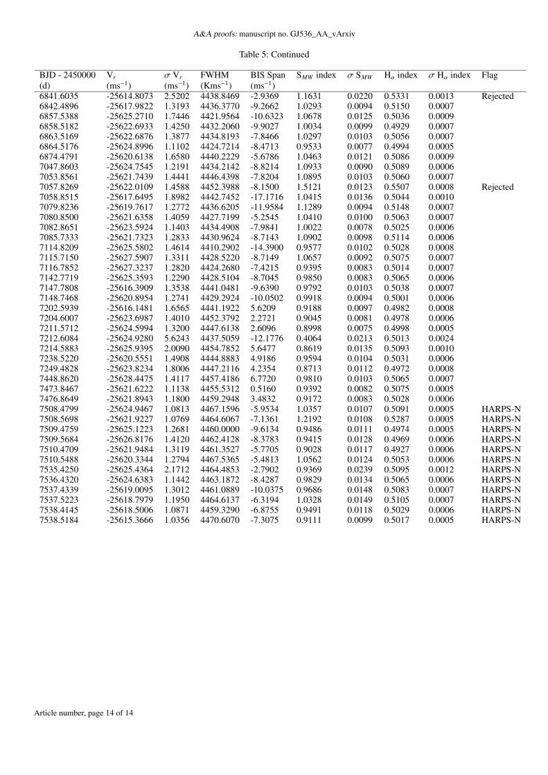
Table 5: Continued

BJD - 2450000 Vr σ Vr FWHM BIS Span SMW index σ SMW Hα index σ Hα index Flag(d) (ms−1) (ms−1) (Kms−1) (ms−1)6841.6035 -25614.8073 2.5202 4438.8469 -2.9369 1.1631 0.0220 0.5331 0.0013 Rejected6842.4896 -25617.9822 1.3193 4436.3770 -9.2662 1.0293 0.0094 0.5150 0.00076857.5388 -25625.2710 1.7446 4421.9564 -10.6323 1.0678 0.0125 0.5036 0.00096858.5182 -25622.6933 1.4250 4432.2060 -9.9027 1.0034 0.0099 0.4929 0.00076863.5169 -25622.6876 1.3877 4434.8193 -7.8466 1.0297 0.0103 0.5056 0.00076864.5176 -25624.8996 1.1102 4424.7214 -8.4713 0.9533 0.0077 0.4994 0.00056874.4791 -25620.6138 1.6580 4440.2229 -5.6786 1.0463 0.0121 0.5086 0.00097047.8603 -25624.7545 1.2191 4434.2142 -8.8214 1.0933 0.0090 0.5089 0.00067053.8561 -25621.7439 1.4441 4446.4398 -7.8204 1.0895 0.0103 0.5060 0.00077057.8269 -25622.0109 1.4588 4452.3988 -8.1500 1.5121 0.0123 0.5507 0.0008 Rejected7058.8515 -25617.6495 1.8982 4442.7452 -17.1716 1.0415 0.0136 0.5044 0.00107079.8236 -25619.7617 1.2772 4436.6205 -11.9584 1.1289 0.0094 0.5148 0.00077080.8500 -25621.6358 1.4059 4427.7199 -5.2545 1.0410 0.0100 0.5063 0.00077082.8651 -25623.5924 1.1403 4434.4908 -7.9841 1.0022 0.0078 0.5025 0.00067085.7333 -25621.7323 1.2833 4430.9624 -8.7143 1.0902 0.0098 0.5114 0.00067114.8209 -25625.5802 1.4614 4410.2902 -14.3900 0.9577 0.0102 0.5028 0.00087115.7150 -25627.5907 1.3311 4428.5220 -8.7149 1.0657 0.0092 0.5075 0.00077116.7852 -25627.3237 1.2820 4424.2680 -7.4215 0.9395 0.0083 0.5014 0.00077142.7719 -25625.3593 1.2290 4428.5104 -8.7045 0.9850 0.0083 0.5065 0.00067147.7808 -25616.3909 1.3538 4441.0481 -9.6390 0.9792 0.0103 0.5038 0.00077148.7468 -25620.8954 1.2741 4429.2924 -10.0502 0.9918 0.0094 0.5001 0.00067202.5939 -25616.1481 1.6565 4441.1922 5.6209 0.9188 0.0097 0.4982 0.00087204.6007 -25623.6987 1.4010 4452.3792 2.2721 0.9045 0.0081 0.4978 0.00067211.5712 -25624.5994 1.3200 4447.6138 2.6096 0.8998 0.0075 0.4998 0.00057212.6084 -25624.9280 5.6243 4437.5059 -12.1776 0.4064 0.0213 0.5013 0.00247214.5883 -25625.9395 2.0090 4454.7852 5.6477 0.8619 0.0135 0.5093 0.00107238.5220 -25620.5551 1.4908 4444.8883 4.9186 0.9594 0.0104 0.5031 0.00067249.4828 -25623.8234 1.8006 4447.2116 4.2354 0.8713 0.0112 0.4972 0.00087448.8620 -25628.4475 1.4117 4457.4186 6.7720 0.9810 0.0103 0.5065 0.00077473.8467 -25621.6222 1.1138 4455.5312 0.5160 0.9392 0.0082 0.5075 0.00057476.8649 -25621.8943 1.1800 4459.2948 3.4832 0.9172 0.0083 0.5028 0.00067508.4799 -25624.9467 1.0813 4467.1596 -5.9534 1.0357 0.0107 0.5091 0.0005 HARPS-N7508.5698 -25621.9227 1.0769 4464.6067 -7.1361 1.2192 0.0108 0.5287 0.0005 HARPS-N7509.4759 -25625.1223 1.2681 4460.0000 -9.6134 0.9486 0.0111 0.4974 0.0005 HARPS-N7509.5684 -25626.8176 1.4120 4462.4128 -8.3783 0.9415 0.0128 0.4969 0.0006 HARPS-N7510.4709 -25621.9484 1.3119 4461.3527 -5.7705 0.9028 0.0117 0.4927 0.0006 HARPS-N7510.5488 -25620.3344 1.2794 4467.5365 -5.4813 1.0562 0.0124 0.5053 0.0006 HARPS-N7535.4250 -25625.4364 2.1712 4464.4853 -2.7902 0.9369 0.0239 0.5095 0.0012 HARPS-N7536.4320 -25624.6383 1.1442 4463.1872 -8.4287 0.9829 0.0134 0.5065 0.0006 HARPS-N7537.4339 -25619.0095 1.3012 4461.0889 -10.0375 0.9686 0.0148 0.5083 0.0007 HARPS-N7537.5223 -25618.7979 1.1950 4464.6137 -6.3194 1.0328 0.0149 0.5105 0.0007 HARPS-N7538.4145 -25618.5006 1.0871 4459.3290 -6.8755 0.9491 0.0118 0.5029 0.0006 HARPS-N7538.5184 -25615.3666 1.0356 4470.6070 -7.3075 0.9111 0.0099 0.5017 0.0005 HARPS-N


Documents

A super-Earth Orbiting the Nearby M-dwarf GJ 536 · 7 Instituto de Astrofísica e Ciências do Espaço, Universidade do Porto,CAUP, Rua das Estrelas, 4150-762 Porto, Portugal 8 Departamento