A SunCam online continuing education course Vibration - Modal … · 2017-01-11 · A SunCam online continuing education course Vibration - Modal Analysis by ... everyday object has

A SunCam online continuing education course

Vibration - Modal Analysis

by

Tony L. Schmitz, PhD



www.SunCam.com Copyright 2011 Tony L. Schmitz Page 2 of 55

1. Modal Analysis Let’s begin our discussion with a definition: modal analysis is [the] study of the dynamic properties of structures under vibrational excitation [1]. This may lead us to think of the dynamics of structures such as automobiles, aircraft, spacecraft, and other large complicated systems. A famous example of the importance of considering the dynamics of civil structures is the Tacoma Narrows bridge in Washington state that collapsed in 1940. It failed when the (steady) wind blowing over the bridge caused self-excited vibration, or flutter, in a twisting mode about its centerline; see Fig. 1.1. However, even the most common, everyday object has its own dynamic response. For example, sports equipment, including golf clubs and baseball bats, are subject to vibration due to the impulsive force applied during contact with the ball. Rotating equipment, such as fans and washing machines, can exhibit large vibrations when there is an imbalance in the rotating member. This represents forced vibration. Vibration of three bones within the middle ear play a critical role in transforming sound waves into what we perceive as “sound”. Here we have an example of free vibration. Regardless of the object’s size, shape, or function, we characterize the vibration behavior using a few special descriptors, including natural frequency, mode shape, and frequency response function. A primary objective of this lesson

Modal analysis is [the] study of the dynamic properties of structures under vibrational excitation [1].

Figure 1.1: Photograph of the Tacoma Narrows bridge taken prior to its collapse [2].




is to explore these concepts in detail. We may also consider modal analysis to be the experimental companion of finite element analysis (FEA). While FEA has become an essential tool to aid designers at the modeling stage, it is very often necessary to validate the results. In particular, experimental modal analysis results can be used to confirm decisions about boundary conditions, material properties, and mesh density. In this lesson, we will begin with a review of the fundamentals of single and two degree of freedom free and forced vibrations and, in doing so, we will establish notation conventions for a description of modal analysis. This will provide us with the basis we need to describe techniques for frequency response function measurement and model development. 1.1 Single degree of freedom free vibration The vibration of bodies that possess both mass and elasticity, or the ability to deform without permanently changing shape, can be divided into three main categories: free, forced, and self-excited vibrations.

Important concepts in modal analysis are natural frequency, mode shape, and frequency response function.

The three categories of vibration are: free, forced, and self-excited.




Free vibration Free vibration occurs in the absence of a long term, external excitation force. It is the result of some initial conditions imposed on the system, such as a displacement from the system’s equilibrium position. Free vibration produces motion in one or more of the system’s natural frequencies and, because all physical structures exhibit some form of damping (or energy dissipation), it is seen as a decaying oscillation with a relatively short duration; see Fig. 1.1.1.

Familiar examples include plucking a guitar string or striking a tuning fork. Forced vibration Forced vibration takes place when a continuous, external periodic excitation produces a response with the same frequency as the forcing function (after the decay of initial transients). While free vibration is often represented in the time domain, forced vibration is typically analyzed in the frequency domain. This emphasizes the magnitude and phase dependence on frequency and enables the convenient identification of natural frequencies. A typical source of forced vibration in mechanical systems is rotating imbalance. Large

vibrations occur when the forcing frequency, , is near a system natural frequency, n, as shown in Fig. 1.1.2. This condition is referred to as resonance and is generally avoided.

0 0.02 0.04 0.06 0.08 0.1-1

-0.5

0

0.5

1

t (s)

x (m

m)

Figure 1.1.1: Damped free vibration example.




Self-excited vibration In self-excited vibration, a steady input force is present, as in the case of forced vibration. However, this input is modulated into vibration at one of the system’s natural frequencies, as with free vibration. The physical mechanisms that provide this modulation are varied. Common examples of self-excited vibration include playing a violin, flutter in airplane wings (or bridges, as shown in Fig. 1.1), and chatter in machining. Let’s begin our discussion of single degree of freedom free vibration with a simple, lumped parameter model. In this model, all the mass is assumed to be concentrated at the coordinate location and the spring that provides the oscillating restoring force is massless. The model is composed of a mass, m, attached to a linear spring, k, that provides a force proportional to its displacement from the mass’s static equilibrium position. Because the rigid mass is only allowed to move vertically, a single time dependent coordinate, x, is sufficient to describe its motion. See Fig. 1.1.3, which includes the free body diagram. Summing the spring and inertial forces in the vertical direction yields the model’s equation of motion:

0 kxxm . (1.1.1)

Figure 1.1.2: Example of forced vibration magnitude.

0 500 1000 1500 2000 25000

1

2

3

4

5

x 10-6

Frequency (rad/s)

Ma

gn

itud

e (

m/N

)

= n




By assuming a harmonic solution of the form stXex , where X is a complex coefficient,

is , and is the frequency (in rad/s), we can express the velocity as the first time

derivative of the displacement, stst XeisXex , and the acceleration as the second time

derivative, stst XeXesx 22 (note that 1i and 12 i ). Substitution into Eq. 1.1.1 gives:

02 kmsXest . (1.1.2)

In this equation, either stXe or kms 2 is zero. If the first term is zero, this means that no

motion has occurred and it is described as the trivial solution. We are interested in the case that the second term is equal to zero. This is referred to as the characteristic equation for the system:

02 kms . (1.1.3)

Solving for the complex variable s gives the two roots m

ki

m

ks . The vibrating

frequency nm

k is the natural frequency for the single degree of freedom system.

Typical SI units for k and m are N/m and kg, respectively, which gives units of rad/s for n .

m

k

x

Figure 1.1.3: Single degree of freedom, undamped lumped parameter model (left); free body diagram (right).

m

x

kx

xm




Alternately, the natural frequency may be expressed in units of Hz (cycles/s). In this case,

we’ll use the notation 2

nnf .

The total solution to Eq. 1.1.1 is the sum of the contributions from each of the two roots:

titi nn eXeXx 21 . (1.1.4)

The complex coefficients, 1X and 2X , can be determined from the initial displacement, 0x ,

and velocity, 0x , of the single degree of freedom system. Evaluating Eq. 1.1.4 at 0t

gives:

210 XXx . (1.1.5)

The first time derivative of Eq. 1.1.4 is:

tin

tin

nn eXieXix 21 . (1.1.6)

At 0t , Eq. 1.1.6 becomes:

210 XiXix nn . (1.1.7)

Equations 1.1.5 and 1.1.7 can be combined to determine the complex conjugate coefficients

1X and 2X :

n

n xxiX

200

1

and (1.1.8)

n

n xxiX

200

2

. (1.1.9)

These coefficients can then be substituted in Eq. 1.1.4 to determine the time dependent displacement of the mass due to the imposed initial conditions. Alternately, the mass motion can be expressed in exponential form. To use this notation, we first need to identify the real (Re) and imaginary (Im) parts of the complex coefficients:




2

Re 01

xX

n

xX

2Im 0

1

(1.1.10)

2

Re 02

xX

n

xX

2Im 0

2

. (1.1.11)

These real and imaginary parts can then be used to write the coefficients in exponential form:

nn

n

n

n

i

x

xi

xxX

x

x

ixx

X

X

XiXXAeX

0

012

20

220

1

0

0

1

2

0

2

01

1

1121

211

tanexp4

2

2tanexp

22

Re

ImtanexpImRe

(1.1.12)

where the magnitude is 2

20

220

4 n

n xxA

and the phase is

nx

x

0

01tan

. Similarly,

iAeX 2 (same magnitude, but negative phase) because it is the complex conjugate of

1X . We can then rewrite the total solution from Eq. 1.1.4 in the form:

tititiitii nnnn eeAeAeeAex . (1.1.13)

Finally, by applying the Euler identity cos2 ii ee , Eq. 1.1.13 can be rewritten as:

tAx ncos2 . (1.1.14)

While Eq. 1.1.14 emphasizes the oscillatory nature of the mass motion and the dependence of the magnitude and phase on the initial conditions, we must also include damping in our analysis in order to model physical systems. Damping refers to the “leakage” of the input energy into the vibrating system. In other words, not all of the input energy serves to cause




motion. Some of it is dissipated in other ways. A comprehensive model of damping is complicated and not particularly well suited for incorporation into our simple mathematical description of single degree of freedom free vibration. Therefore, one or more of three mathematically simple, but effective, damping models are typically applied. Viscous damping A common assertion is that the retarding damping force is proportional to the mass velocity. You may have experienced this phenomenon if you’ve attempted to force a body through a fluid, such as pulling your hand through water or sticking your hand out the window of a moving vehicle. You probably observed that increasing the speed of your hand relative to the fluid raised the resistance proportionally. If we write the damping force as:

xcf (1.1.15)

and substitute the velocity expression stst XeisXex , we see that viscous damping is frequency dependent. When sketching models of lumped parameter systems, the damping element is often illustrated as a fluid dashpot (similar to a car’s shock absorber) when the viscous damping model is applied. Typical SI units for c are N-s/m. Coulomb damping Another effective damping model is Coulomb damping, or dry sliding friction. Here, energy is dissipated (as heat) due to relative motion between two contacting surfaces. The force magnitude depends on the sliding (kinetic) friction coefficient, , and the normal force, N,

between the two bodies. See Fig. 1.1.4. Because the friction force always opposes the direction of motion, the resulting equation of motion is nonlinear. A piecewise definition1 of the Coulomb damping force is [3]:

1 A piecewise definition is one with separate, non-overlapping, parts.

Damping refers to the “leakage” of the input energy into the vibrating system.




0

0

0

0

x

x

x

N

N

f

. (1.1.16)

Solid damping Even in the absence of an external fluid medium or sliding friction against another surface, the motion of a freely oscillating body decays over time. This is due to energy dissipation internal to the body (perhaps a good mental picture is molecules sliding relative to each other within the body itself during periodic motion and elastic deformation). The energy dissipation during a cycle of motion for this solid or structural damping is taken to be proportional to the square of the vibration magnitude. Using the concept of equivalent viscous damping, solid damping is often incorporated with stiffness to arrive at a complex stiffness term in the differential equation of motion [4]. For the remainder of this lesson, we will use viscous damping to describe energy dissipation in the lumped parameter models. The equation of motion for free vibration of the single degree of freedom spring-mass-damper (Fig. 1.1.5) can then be written as:

0 kxxcxm . (1.1.17)

N

x

f

Figure 1.1.4: Coulomb damping occurs due to dry sliding friction between the two surfaces. The normal and friction forces are shown.




Again assuming the harmonic solution stXex , we obtain the characteristic equation:

02 kcsms , (1.1.18) which can be rewritten as:

02 m

ks

m

cs . (1.1.19)

This equation is quadratic in s2 and has the two roots:

m

k

m

c

m

cs

2

2,1 22. (1.1.20)

The vibratory behavior of the spring-mass-damper depends on the term under the radical in

Eq. 1.1.20. If 02

2

m

k

m

c, the system is underdamped and vibratory. If 0

2

2

m

k

m

c,

the system is said to be critically damped and, if 02

2

m

k

m

c, then the system is

overdamped. For these two cases, no vibration (oscillation) occurs. Because the damping is

m

k

x

Figure 1.1.5: Single degree of freedom, damped lumped parameter model (left); free body diagram (right).

c m

x

kx

xm

xc




generally low in mechanical systems, we will consider only the underdamped option in our analyses. For underdamped systems, Eq. 1.1.20 can be rewritten as:

dn is 2,1 , (1.1.21)

where we’ve introduced the dimensionless

damping ratio, km

c

2 , and damped natural

frequency, 21 nd . Under the viscous

damping assumption, we see that the free vibrating frequency is reduced in the presence of damping. However, for typical mechanical systems, the damping is low enough that the frequency change is negligible. Using the two roots in Eq. 1.1.21, the total solution for the free motion of the single degree of freedom spring-mass-damper is:

titittiti ddndndn eXeXeeXeXx 2121 . (1.1.22)

Like the undamped case, the complex coefficients can be determined from the initial

conditions. Taking the time derivative of Eq. 1.1.22, substituting the initial displacement, 0x ,

and velocity, 0x , and solving for 1X and 2X gives the complex conjugate pair:

d

n xxi

xX

22000

1

and

d

n xxi

xX

22000

2

. (1.1.23)

Using these coefficients, the exponential form can again be developed in a similar way to Eq.

1.1.12 by substituting for the real and imaginary parts. For example, 2

Re 01

xX and

d

n xxX

2Im 00

1

for the coefficient 1X . Note that these terms simplify to Eq. 1.1.10

for the undamped case if is set equal to zero.

1.2 Single degree of freedom forced vibration

Mechanical systems can be underdamped, critically damped, or overdamped. Most systems are underdamped, which means that they will oscillate during free vibration.




We will again consider the spring-mass-damper model shown in Fig. 1.1.5. However, a

harmonic external force is now applied to the mass. The force is shown as tife in Fig. 1.2.1.

The corresponding equation of motion is:

fkxxcxm . (1.2.1)

Although the total solution to Eq. 1.2.1 includes both the homogeneous (transient) and particular (steady state) components, we have already described the damped transient response in the previous section. We will therefore consider only the steady state solution here. Because the motion response has the same frequency as the forcing function, we can

assume a solution of the form tiXex . The velocity and acceleration can then be written as tiXeix and tiXex 2 . Substituting in Eq. 1.2.1 gives:

titi feXekcim 2 . (1.2.2)

Rewriting Eq. 1.2.2 gives the complex valued frequency response function (FRF). We will use this description of Eq. 1.2.3, rather than transfer function, because we can only consider

m

k

x

Figure 1.2.1: Single degree of freedom, lumped parameter model (damped with force).

c

tife

The total solution to forced vibration includes both transient and steady state components.




positive frequencies and a single system configuration (damping and natural frequency) when we perform measurements. The term transfer function refers to the theoretical situation

where all frequencies ( to ) and n combinations are included.

kicmF

X

2

1 (1.2.3)

There are two primary ways to represent the complex function shown in Eq. 1.2.3. The first is to separate the function into its magnitude and phase components and the second is to express the function using its real and imaginary parts. The frequency dependent magnitude and phase are written as:

222

21

11

nn

kF

X

and (1.2.4)

2

11

1

2

tanRe

Imtan

n

n

F

XF

X

. (1.2.5)

Because Eqs. 1.2.4 and 1.2.5 are somewhat cumbersome, it is common to replace the

frequency ratio n

with another variable, such as r. We will also adopt this convention. The

real and imaginary parts of the FRF are provided in Eqs. 1.2.6 and 1.2.7.

222

2

21

11Re

rr

r

kF

X

(1.2.6)

222 21

21Im

rr

r

kF

X

(1.2.7)

Example 1.2.1: FRF for single degree of freedom system




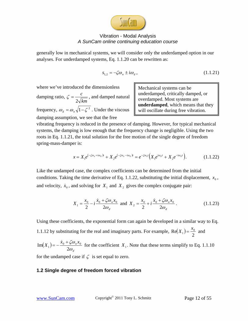
Let’s consider a single degree of freedom spring-mass-damper system with a mass of 1 kg, a

spring constant of 6101 N/m, and a viscous damping coefficient of 200 N-s/m. In order to apply Eqs. 1.2.4-1.2.7, we must calculate the (undamped) natural frequency and damping ratio.

10001

101 6

m

kn rad/s

1.011012

200

2 6

km

c

Figure 1.2.2 shows the magnitude and phase as a function of the frequency ratio, r. Although a logarithmic magnitude axis (i.e., a semilog plot) is often shown in the literature, we will use a linear convention for plots unless specified otherwise. The real and imaginary parts are provided in Fig. 1.2.3. Note that the zero frequency (DC) value for both the real part and

magnitude is 61011 k

m/N. This represents the real valued static deflection of the spring

(away from its equilibrium position) under a unit force. We can also see that the magnitude at

resonance ( 1r or n ) is significantly larger than the DC deflection. This magnitude is

61052

1 k

m/N.




The maximum value of the real part occurs at 21r , which we will approximate as

Figure 1.2.2: Magnitude and phase for example single degree of freedom system.

0 0.5 1 1.5 20

2

4

x 10-6

Ma

gn

itud

e (

m/N

)

0 0.5 1 1.5 2

-150

-100

-50

0

r

Ph

ase

(d

eg

)

0 0.5 1 1.5 2

-2

0

2

x 10-6

Re

al (

m/N

)

0 0.5 1 1.5 2

-4

-2

0x 10

-6

r

Ima

g (

m/N

)

r = 0.9

r = 1.1

Figure 1.2.3: Real and imaginary parts for example single degree of freedom system.




9.01 r (this approximation is valid for small values when 2 is negligible). The

minimum real part occurs at 21r , approximated as 1.11 r . The difference in

the real value between these maximum and minimum points is the same as the magnitude

peak value 61052

1 k

m/N. The imaginary minimum is seen at resonance with a value

of 61052

1 k

m/N.

In addition to the frequency dependent representations of the FRF shown in Figs. 1.2.2 and 1.2.3, the Argand diagram can also be selected. In this case, the real part is graphed versus the imaginary part (i.e., the complex plane) and the same information identified in the previous paragraphs is compactly represented. As we traverse the “circle” clockwise from

0r , where the real part is 61011 k

m/N and the imagnary part is zero, we sequentially

encounter the 9.01 r point where the real part is maximum, the 1r point where

the real part is zero and the imaginary part is most negative, the 1.11 r point where

the real part is most negative, and, finally, we approach the r frequency ratio where both the real and imaginary parts are zero.

-3 -2 -1 0 1 2 3

x 10-6

-5

-4

-3

-2

-1

0

x 10-6

Real (m/N)

Ima

g (

m/N

)

r = 0

r = 0.9

r = 1

r = 1.1

Figure 1.2.4: Argand diagram for example single degree of freedom system.




Using a vector representation for F

X, the magnitude is identified as the length of the vector

which extends from the origin to any point (i.e., a desired r value) on our “circle”. The phase lag between the displacement and force is the angle between the vector and the positive real axis. The real and imaginary parts are simply the projections of the vector on the real and imaginary axes.

1.3 Two degree of freedom free vibration We will again use the lumped parameter spring-mass-damper model as the basis for our discussion, but we will now include a second degree of freedom by adding a second spring-mass-damper to the first in a “chain-type” configuration; see Fig. 1.3.1. Using the free body diagrams for the top and bottom masses, where inertial forces are shown in addition to the spring and viscous damper forces, the two equations of motion can be written by equating the sum of the forces in the vertical direction to zero. The equation of motion for the top mass is:

0222212112111 xkxcxkkxccxm (1.3.1)

and the equation of motion for the bottom mass is:

Figure 1.2.5: Vector representation of FRF in the complex plane.

-3 -2 -1 0 1 2 3

x 10-6

-5

-4

-3

-2

-1

0

x 10-6

Real (m/N)

Ima

g (

m/N

)

Re

Im




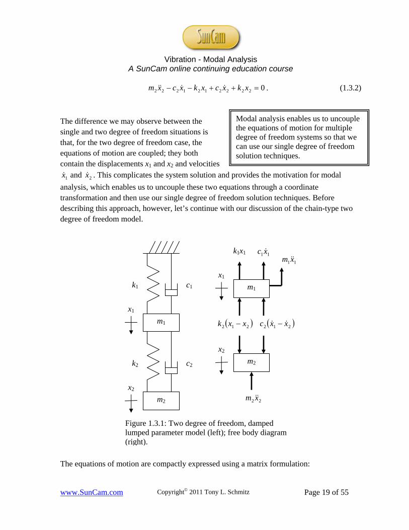
02222121222 xkxcxkxcxm . (1.3.2)

The difference we may observe between the single and two degree of freedom situations is that, for the two degree of freedom case, the equations of motion are coupled; they both contain the displacements x1 and x2 and velocities

1x and 2x . This complicates the system solution and provides the motivation for modal

analysis, which enables us to uncouple these two equations through a coordinate transformation and then use our single degree of freedom solution techniques. Before describing this approach, however, let’s continue with our discussion of the chain-type two degree of freedom model.

The equations of motion are compactly expressed using a matrix formulation:

m1

k1

x1

Figure 1.3.1: Two degree of freedom, damped lumped parameter model (left); free body diagram (right).

c1

m2

k2

x2

c2

m1

x1

212 xxc 212 xxk

11xm

m2

x2

22 xm

k1x1 11xc

Modal analysis enables us to uncouple the equations of motion for multiple degree of freedom systems so that we can use our single degree of freedom solution techniques.




0

0

0

0

2

1

22

221

2

1

22

221

2

1

2

1

x

x

kk

kkk

x

x

cc

ccc

x

x

m

m

. (1.3.3)

The coupling is seen to occur in the symmetric damping and stiffness matrices for this chain-type model due to the nonzero off-diagonal terms in the matrix positions (1,2) and (2,1). If

we represent the mass and stiffness matrices as M and K , neglect damping for now, and

assume a harmonic solution of the form stXex , we can write:

02 steXKsM . (1.3.4)

Similar to Eq. 1.1.2, there are two possibilities for the product in Eq. 1.3.4. If 0X , we

obtain the trivial solution. We are therefore interested in the case when 02 KsM .

From linear algebra [5], we know that for this matrix of equations to have a non-trivial solution, the determinant must be equal to zero. This represents the characteristic equation for our system.

02 KsM (1.3.5)

The determinant of a two row, two column (2x2) matrix can be calculated by finding the difference between the products of the on-diagonal (1,1 and 2,2) terms and the off-diagonal terms. This is expressed generically as:

022

22

fesdcs

dcsbas or (1.3.6)

02222 dcsfesbas . (1.3.7)

This equation is quadratic in s2, i.e., 024 mhsgs , and we can find the roots, 21s and

22s , using the quadratic equation. These two roots are the eigenvalues for the two degree of

freedom system. The natural frequencies are calculated as:

21

21 ns and 2

22

2 ns , (1.3.8)




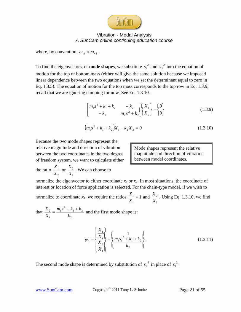
where, by convention, 21 nn .

To find the eigenvectors, or mode shapes, we substitute 21s and 2

2s into the equation of

motion for the top or bottom mass (either will give the same solution because we imposed linear dependence between the two equations when we set the determinant equal to zero in Eq. 1.3.5). The equation of motion for the top mass corresponds to the top row in Eq. 1.3.9; recall that we are ignoring damping for now. See Eq. 1.3.10.

0

0

2

1

22

22

2212

1

X

X

ksmk

kkksm (1.3.9)

0221212

1 XkXkksm (1.3.10)

Because the two mode shapes represent the relative magnitude and direction of vibration between the two coordinates in the two degree of freedom system, we want to calculate either

the ratio 2

1

X

X or

1

2

X

X. We can choose to

normalize the eigenvector to either coordinate x1 or x2. In most situations, the coordinate of interest or location of force application is selected. For the chain-type model, if we wish to

normalize to coordinate x1, we require the ratios 11

1 X

X and

1

2

X

X. Using Eq. 1.3.10, we find

that 2

212

1

1

2

k

kksm

X

X and the first mode shape is:

2

212

11

1

2

1

1

1

1

k

kksm

X

XX

X

. (1.3.11)

The second mode shape is determined by substitution of 22s in place of 2

1s :

Mode shapes represent the relative magnitude and direction of vibration between model coordinates.




2

212

21

1

2

1

1

2

1

k

kksm

X

XX

X

. (1.3.12)

The first mode shape corresponds to vibration in the first natural frequency 1n , while the

second mode shape is associated with vibration at 2n . In general, the system will vibrate in

a linear combination of both mode shapes/natural frequencies, depending on the initial

conditions. If we’ve followed the convention of 21 nn and normalized to the x1

coordinate, we’ll find that the first mode shape will take the form

0

11 a

, where a is a

real number, which indicates that the two masses are vibrating exactly in phase with one another (i.e., they reach their maximum and minimum displacements at the same instants in time). We’ll also see that the second mode

shape will take the form

0

12 a

, which means that the mass motions are exactly out of

phase with one another (i.e., when one mass reaches its maximum displacement, the other is at its minimum displacement). Example 1.3.1: Free vibration using complex coefficients In this example we will calculate the time response of the system in Fig. 1.3.1 when the mass

values are 11 m kg and 5.02 m kg, the stiffness values are 71 101k N/m and

72 102k N/m, the initial displacement of 1x is 11,0 x mm and the initial displacement of

2x is 12,0 x mm, and the initial velocities are zero. The equations of motion in matrix

form are:

0

0

102102

102102101

5.00

01

2

1

77

777

2

1

x

x

x

x

.

The characteristic equation is:

The first mode shape corresponds to vibration in the first natural frequency. The second mode shape oscillates at the second natural frequency and so on.




01025.0102

1021031727

772

s

s, or 0102105.35.0 14274 ss .

This equation yields the two roots 621 10277.6 s (rad/s)2 and 72

2 10372.6 s (rad/s)2,

which give the natural frequencies 2505211 sn rad/s and 79832

22 sn

rad/s. Expressed in units of Hz, these natural frequencies are 8.3982

11

n

nf Hz and

12712

22

n

nf Hz.

Let’s normalize the mode shapes to x2 and arbitrarily select the equation of motion for the top

mass to calculate the ratio 72

7

2

1

1031

102

sX

X. We obtain the first mode shape, which

corresponds to vibration in 1n , by substituting 21s in this ratio:

1

8431.0

110310277.6

10276

7

2

2

2

1

1

X

XX

X

.

See Fig. 1.3.2, where the relative deflection amplitudes between coordinates 1 and 2 are

identified. The second mode shape, which corresponds to vibration in 2n , is:

1

5931.0

110310372.6

10277

7

2

2

2

1

2

X

XX

X

.

See Fig. 1.3.3, where the deflections are now in opposite directions (out of phase). Similar to Eq. 1.1.4, we can generically write the time domain solution for the x1 and x2 vibrations as:

titititi eXeXeXeXx 7983*12

798312

2505*11

2505111

and titititi eXeXeXeXx 7983*

227983

222505*

212505

212 .




0.8431

1

Figure 1.3.2: Mode shape 1 normalized to coordinate 2.

m1

x1

m2

x2

-0.5931

1

Figure 1.3.3: Mode shape 2 normalized to coordinate 2.

x1

m2

x2

m1




Here, ijX and *ijX represent a complex conjugate pair, where the subscript i indicates the

coordinate number and the subscript j denotes the natural frequency number. This solution suggests the general case that the total vibration is a linear combination of vibration in each of the two modes. The first time derivatives are:

titititi eXeXieXeXix 7983*12

798312

2505*11

2505111 79832505 and

titititi eXeXieXeXix 7983*22

798322

2505*21

2505212 79832505 .

Substitution of the initial conditions leads to a system of four equations with eight unknowns.

*

2222*

21212,0

*1212

*11111,0

*2222

*21212,0

*1212

*11111,0

798325050

798325050

1

1

XXiXXix

XXiXXix

XXXXx

XXXXx

However, we can apply the mode shape relationships to reduce this to a system of four

equations with four unknowns. Using the same definitions for the ijX subscripts, we can

write 8431.021

11 X

X and 5931.0

21

11 X

X. After substitution and rewriting in matrix form, we

obtain:

0

0

1

1

7983798325052505

4734473421122112

1111

5931.05931.08431.08431.0

*22

22

*21

21

X

X

X

X

iiii

iiii, or bXA .

We can determine the coefficients by inverting A and premultiplying b by this result,

bAX 1 . The result is

6417.0

6417.0

1417.0

1417.0

*22

22

*21

21

X

X

X

X

. Using these values and the mode shape




relationships to obtain the remaining four coefficients, we can substitute in the original x1 and x2 expressions to determine the time dependent free vibration for our example system.

titititi eeeex 79837983250525051 3805.03805.01194.01194.0

titititi eeeex 79837983250525052 6417.06417.01417.01417.0

Further, we can use the Euler identity cos2 ii ee to rewrite x1 and x2 as a sum of

cosines. It is seen that the final motion of each mass is a linear combination of vibration in the two natural frequencies.

ttx 7983cos7610.02505cos2388.01

ttx 7983cos283.12505cos2834.02

A potential problem with this approach is that, for additional degrees of freedom, the size of the matrix varies with the square of the number of coordinates. For example, we inverted a 22x22, or 4x4, complex matrix for our two degree of freedom system. For a three degree of freedom model, it would be necessary to invert a 32x32, or 9x9, complex matrix, and so on. While computational capabilities continually increase, modal analysis offers an alternative to this approach. The fundamental idea behind modal analysis is that a coordinate transformation is applied to convert from the model, or local, coordinate system into a modal coordinate system. While these modal coordinates do not have physical significance, they lead to uncoupled equations of motion because the off-diagonal terms in the mass and stiffness matrices are zero. The coordinate transformation is a diagonalization process and relies upon the orthogonality of the eigenvectors. Let’s rework Example 1.3.1 to demonstrate the modal analysis approach. Example 1.3.2: Free vibration by modal analysis The first step in the modal analysis approach is typically to find the eigensolution (natural frequencies and mode shapes). However, we have already completed this step in the previous

example. Our next task is to define the modal matrix, P . It is a square matrix whose

columns are composed of the mode shapes,

11

5931.08431.021 P , where

The fundamental idea behind modal analysis is that a transformation is applied to convert from a local into a modal coordinate system. The modal coordinates are then uncoupled.




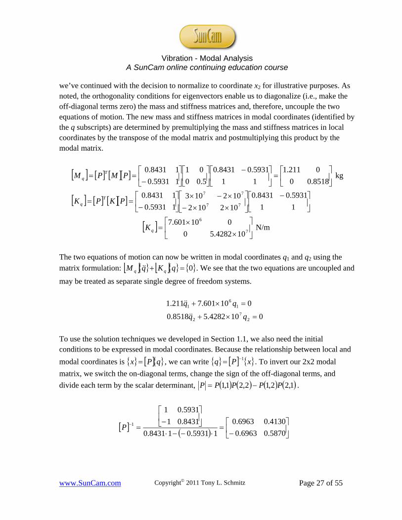
we’ve continued with the decision to normalize to coordinate x2 for illustrative purposes. As noted, the orthogonality conditions for eigenvectors enable us to diagonalize (i.e., make the off-diagonal terms zero) the mass and stiffness matrices and, therefore, uncouple the two equations of motion. The new mass and stiffness matrices in modal coordinates (identified by the q subscripts) are determined by premultiplying the mass and stiffness matrices in local coordinates by the transpose of the modal matrix and postmultiplying this product by the modal matrix.

8518.00

0211.1

11

5931.08431.0

5.00

01

15931.0

18431.0PMPM T

q kg

11

5931.08431.0

102102

102103

15931.0

18431.077

77

PKPK Tq

7

6

104282.50

010601.7qK N/m

The two equations of motion can now be written in modal coordinates q1 and q2 using the

matrix formulation: 0 qKqM qq . We see that the two equations are uncoupled and

may be treated as separate single degree of freedom systems.

010601.7211.1 16

1 qq

0104282.58518.0 27

2 qq

To use the solution techniques we developed in Section 1.1, we also need the initial conditions to be expressed in modal coordinates. Because the relationship between local and

modal coordinates is qPx , we can write xPq 1 . To invert our 2x2 modal

matrix, we switch the on-diagonal terms, change the sign of the off-diagonal terms, and

divide each term by the scalar determinant, 1,22,12,21,1 PPPPP .

5870.06963.0

4130.06963.0

15931.018431.0

8431.01

5931.01

1P




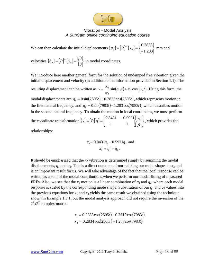
We can then calculate the initial displacements

283.1

2833.00

10 xPq mm and

velocities

0

00

10 xPq in modal coordinates.

We introduce here another general form for the solution of undamped free vibration given the initial displacement and velocity (in addition to the information provided in Section 1.1). The

resulting displacement can be written as txtx

x nnn

cossin 00

. Using this form, the

modal displacements are ttq 2505cos2833.02505sin01 , which represents motion in

the first natural frequency, and ttq 7983cos283.17983sin02 , which describes motion

in the second natural frequency. To obtain the motion in local coordinates, we must perform

the coordinate transformation

2

1

11

5931.08431.0

q

qqPx , which provides the

relationships:

211 5931.08431.0 qqx and

212 qqx .

It should be emphasized that the x2 vibration is determined simply by summing the modal displacements, q1 and q2. This is a direct outcome of normalizing our mode shapes to x2 and is an important result for us. We will take advantage of the fact that the local response can be written as a sum of the modal contributions when we perform our modal fitting of measured FRFs. Also, we see that the x1 motion is a linear combination of q1 and q2, where each modal response is scaled by the corresponding mode shape. Substitution of our q1 and q2 values into the previous equations for x1 and x2 yields the same result we obtained using the technique shown in Example 1.3.1, but the modal analysis approach did not require the inversion of the 22x22 complex matrix.

ttx 7983cos7610.02505cos2388.01

ttx 7983cos283.12505cos2834.02




The final consideration in this section is solution of the two degree of freedom free vibration problem in the presence of damping. We’ve already stated that every physical system dissipates energy, so our analysis should incorporate the viscous damping matrix shown in Eq. 1.3.3. However, this complicates the eigensolution. At this point, we need to introduce the concept of proportional damping. Physically, proportional damping means that all the coordinates pass through their equilibrium (zero) positions at the same instant for each mode shape. For the low damping observed in the typical mechanical assemblies we will be considering, this assumption is realistic. For very high damping values, however, it is less reasonable because there may be significant phase differences between the motions of individual coordinates. Mathematically, proportional damping requires that the damping matrix can be written as a linear combination of the mass and stiffness matrices:

KMC , where and are real numbers.

Provided the proportional damping requirement is satisfied, then damping may be neglected in the eigensolution and the modal analysis procedure follows the steps provided in Example 1.3.2. The only modifications are that we must calculate the modal damping matrix

PCPC Tq and the general solution to the uncoupled modal equations of motion

0 qKqCqM qqq is different. For the underdamped case, we can write

tqt

qqeq dd

d

ntn cossin 0

00 . Otherwise, the solution proceeds as before.

1.4 Two degree of freedom forced vibration We will use the two degree of freedom lumped parameter spring-mass-damper model shown in Fig. 1.3.1, but will impose external harmonic forces at coordinates x1 and x2 for the general case. See Fig. 1.4.1. However, for linear systems we can apply the principle of superposition to consider the forces separately and then sum the individual contributions. For

demonstration purposes, we will consider only the tief 2 force applied to coordinate x2. The

equations of motion in matrix form for this system are:

22

1

22

221

2

1

22

221

2

1

2

1 0

0

0

fx

x

kk

kkk

x

x

cc

ccc

x

x

m

m

. (1.4.1)

Proportional damping means that all the coordinates pass through their equilibrium positions at the same instant for each mode shape. For low damping, this assumption is valid.




By assuming solutions of the form tieXx 2,12,1 and substituting in Eq. 1.4.1, we obtain:

titi eFeXKCiM 2 . (1.4.2)

We have two methods that we can use to determine the steady state forced vibration response for this system. The first is modal analysis, which requires proportional damping, and the second is complex matrix inversion, which places no restrictions on the nature of the system damping. Let’s begin with modal analysis. Modal analysis Our first step in the modal analysis approach is to write the system equations of motion in local coordinates as shown in Eq. 1.4.1; we continue to consider the f2 case in this discussion.

m1

k1

x1

Figure 1.4.1: Two degree of freedom, lumped parameter system (damped with force).

c1

m2

k2

x2

c2

tief 1

tief 2




Provided proportional damping exists (i.e., KMC is true), then we can ignore

damping to find the eigensolution. Note that this solution is also independent of the external force(s). We find the eigenvalues (natural frequencies) and eigenvectors (modes shapes)

using Eq. 1.3.4, 02 steXKsM . The eigenvalues are determined from the roots of

Eq. 1.3.5, 02 KsM . The natural frequencies are computed from 22njjs , j = 1 to

2 (the number of degrees of freedom). We can then use either of the equations of motion to find the 2x1 mode shapes for the two degree of freedom system:

1

21

2

1

1

sX

X and

1

22

2

1

2

sX

X , (1.4.3)

where we have normalized to the location of the force application (coordinate x2). Using the

mode shapes, we assemble the 2x2 modal matrix 21 P . We can then use the modal

matrix to transform into modal coordinates (and uncouple the equations of motion). The

diagonal modal mass, damping, and stiffness matrices are:

2

1

0

0

q

qTq m

mPMPM ,

2

1

0

0

q

qTq c

cPCPC , and

2

1

0

0

q

qTq k

kPKPK , respectively. We must

also transform the local force vector into modal coordinates:

2

2

22

1

222

2

1

21

2

1

2

1 0

1

10

1

1

f

f

fp

p

fsX

X

sX

X

FPR

RR T . (1.4.4)

The modal equations of motion are:

2222222

1111111

Rqkqcqm

Rqkqcqm

qqq

qqq

(1.4.5)

and the corresponding complex FRFs (steady state responses in the frequency domain) are:




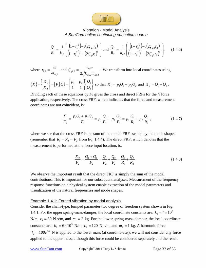
211

221

112

1

11

1

21

211

rr

rir

kR

Q

q

q

q

and

222

222

222

2

22

2

21

211

rr

rir

kR

Q

q

q

q

, (1.4.6)

where 2,1

2,1n

r

and 2,12,1

2,12,1

2 qq

qq

mk

c . We transform into local coordinates using

2

121

2

1

11 Q

QppQP

X

XX so that 22111 QpQpX and 212 QQX .

Dividing each of these equations by F2 gives the cross and direct FRFs for the f2 force application, respectively. The cross FRF, which indicates that the force and measurement coordinates are not coincident, is:

2

22

1

11

2

22

2

11

2

2211

2

1

R

Qp

R

Qp

F

Qp

F

Qp

F

QpQp

F

X

, (1.4.7)

where we see that the cross FRF is the sum of the modal FRFs scaled by the mode shapes

(remember that 221 FRR from Eq. 1.4.4). The direct FRF, which denotes that the

measurement is performed at the force input location, is:

2

2

1

1

2

2

2

1

2

21

2

2

R

Q

R

Q

F

Q

F

Q

F

QQ

F

X

. (1.4.8)

We observe the important result that the direct FRF is simply the sum of the modal contributions. This is important for our subsequent analyses. Measurement of the frequency response functions on a physical system enable extraction of the model parameters and visualization of the natural frequencies and mode shapes. Example 1.4.1: Forced vibration by modal analysis Consider the chain-type, lumped parameter two degree of freedom system shown in Fig.

1.4.1. For the upper spring-mass-damper, the local coordinate constants are: 51 104k

N/m, 801 c N-s/m, and 21 m kg. For the lower spring-mass-damper, the local coordinate

constants are: 52 106k N/m, 1202 c N-s/m, and 12 m kg. A harmonic force

tief 1002 N is applied to the lower mass (at coordinate x2); we will not consider any force

applied to the upper mass, although this force could be considered separately and the result




added to the solution of the analysis we will perform here. The local mass, damping, and

stiffness matrices are:

10

02M kg,

120120

120200C N-s/m, and

55

56

106106

106101K N/m, respectively. To use modal analysis, we must verify that

proportional damping exists. For 0 and 5000

1 , we see that the relationship

KMC is satisfied. We can therefore determine the eigenvalues using:

0106106

1061012525

562

s

s.

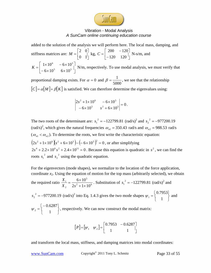
The two roots of the determinant are: 81.12279921 s (rad/s)2 and 19.9772002

2 s

(rad/s)2, which gives the natural frequencies 43.3501 n rad/s and 53.9882 n rad/s

( 21 nn ). To determine the roots, we first write the characteristic equation:

01061061012255262 ss , or after simplifying

0104.2102.22 11264 ss . Because this equation is quadratic in 2s , we can find the

roots 21s and 2

2s using the quadratic equation.

For the eigenvectors (mode shapes), we normalize to the location of the force application, coordinate x2. Using the equation of motion for the top mass (arbitrarily selected), we obtain

the required ratio 62

5

2

1

1012

106

sX

X. Substitution of 81.1227992

1 s (rad/s)2 and

19.97720022 s (rad/s)2 into Eq. 1.4.3 gives the two mode shapes

1

7953.01 and

1

6287.02 , respectively. We can now construct the modal matrix:

11

6287.07953.021 P

and transform the local mass, stiffness, and damping matrices into modal coordinates:




790.10

0265.2PMPM T

q kg,

6

5

10750.10

010782.2PKPK T

q N/m , and

9.3490

063.55PCPC T

q N-s/m.

A simple check at this point is to recalculate the natural frequencies using the modal parameters. The results should match the eigenvalue solution. Here, we see that

46.350265.2

10782.2 5

1

11

q

qn m

k rad/s and 76.988

790.1

10750.1 6

2

22

q

qn m

k rad/s,

where the differences are due to round-off error, but the results are essentially the same. We can also determine the modal damping ratios:

035.0265.210782.22

63.55

2 511

11

qq

qq

mk

c (3.5% damping) and

099.0790.110750.12

9.349

2 622

22

qq

qq

mk

c (9.9% damping).

To write our uncoupled equations of motion in modal coordinates, we also need the modal force vector, which we obtain by substitution into Eq. 1.4.4.

100

100

100

0

16287.0

17953.0R N

10010750.19.349790.1

10010782.263.55265.2

26

22

15

11

qqq

qqq

The FRFs for the single degree of freedom modal systems are:

2

1

221

12

15

1

1

070.01

070.01

10782.2

1

rr

rir

R

Q and

2

2

222

22

26

2

2

198.01

198.01

10750.1

1

rr

rir

R

Q,




where 43.3501

r and

53.9882

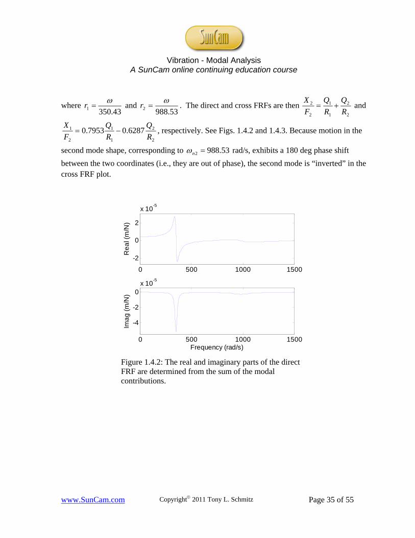
r . The direct and cross FRFs are then

2

2

1

1

2

2

R

Q

R

Q

F

X and

2

2

1

1

2

1 6287.07953.0R

Q

R

Q

F

X , respectively. See Figs. 1.4.2 and 1.4.3. Because motion in the

second mode shape, corresponding to 53.9882 n rad/s, exhibits a 180 deg phase shift

between the two coordinates (i.e., they are out of phase), the second mode is “inverted” in the cross FRF plot.

0 500 1000 1500

-2

0

2

x 10-5

Re

al (

m/N

)

0 500 1000 1500

-4

-2

0x 10

-5

Frequency (rad/s)

Ima

g (

m/N

)

Figure 1.4.2: The real and imaginary parts of the direct FRF are determined from the sum of the modal contributions.




Complex matrix inversion Our final task of this section is to describe an alternative to modal analysis, referred to as complex matrix inversion. This approach does not require proportional damping, but does include the inversion of a 2x2 frequency dependent, complex matrix for the two degree of

freedom system we are considering here. We’ll first write Eq. 1.4.2 in the form FXA ,

where KCiMaa

aaA

2

2221

1211 . The two degree of freedom system has

four FRFs that we’d like to determine. First, we have the direct and cross FRFs, 2

2

F

X and

2

1

F

X, due to the force application at coordinate 2x that we previously determined using

modal analysis. Second, we have the direct and cross FRFs, 1

1

F

X and

1

2

F

X, due to the force

application at coordinate 1x . We did not explicitly show the modal solution to this case, but

the only differences are that we would normalize the mode shapes to 1x and the FRFs would

0 500 1000 1500

-2

0

2

x 10-5

Re

al (

m/N

)

0 500 1000 1500

-4

-2

0x 10

-5

Frequency (rad/s)

Ima

g (

m/N

)

Figure 1.4.3: The real and imaginary parts of the cross FRF are obtained by scaling the two modes by the corresponding mode shape and summing the results.




then be computed from 2

2

1

1

1

1

R

Q

R

Q

F

X and

2

22

1

11

1

2

R

Qp

R

Qp

F

X , where

21

11

ppP

would be used to determine the modal mass, stiffness, and damping matrices.

Rewriting FXA as 11 AFX provides all four FRFs. They are ordered as:

2221

1211

2

2

1

2

2

1

1

1

bb

bb

F

X

F

XF

X

F

X

, where we’ve used the bij notation to indicate the individual terms

in the inverted A matrix. In our analysis, A is symmetric. Therefore, 2112 bb and

1

2

2

1

F

X

F

X . This condition is referred to as reciprocity. Physically, it means that we get the

same result if we: 1) excite the system at

coordinate 2x and measure the response at 1x ,

as if we: 2) excite the system at coordinate 1x

and measure the response at 2x .

For the two degree of freedom system, we can directly write the individual terms in 1A as:

21122211

212112

22

222222

21122211

1121

1222

1

aaaa

kkccimkci

kcikcim

aaaa

aa

aa

A

.

For example, 21122211

2222

111

1

aaaa

kcimb

F

X

. Note that this complex expression is a

function of the forcing frequency so it must be evaluated over the desired frequency range in order to produce plots equivalent to those obtained for the modal analysis example. 1.5 System identification The previous section describes the modal analysis steps required to obtain the direct and cross FRFs in local coordinates given a system model (we treated the chain-type, lumped parameter case, but other model geometries could be considered as well). This approach required that the mass, damping, and stiffness matrices be known. However, this is not the

Reciprocity means that we get the same FRF if we: 1) excite at coordinate i and measure at coordinate j; or 2) if we excite at j and measure at i.




case for arbitrary structures. Our actual task is typically to measure the FRFs for the system of interest and then define a model by performing a modal fit to the measured data. Modal fitting Our fitting approach will be a “peak picking” method where we use the real and imaginary parts of the system FRFs to identify the modal parameters [6]. This approach works well provided the system modes are not closely spaced. However, even if two modeled modes are relatively close in frequency, we can still obtain a reasonable modal fit as we’ll see in Example 1.5.1.

To demonstrate the fitting steps, consider the direct FRF shown in Fig. 1.5.1. This FRF clearly has two modes within the measurement bandwidth. To determine the modal parameters which populate the 2x2 modal matrices, we must identify three frequencies and one peak value for each mode. [Note that we have automatically assumed proportional damping in using this approach. Additionally, if there were three dominant modes we wished to model, we would obtain 3x3 modal matrices and so on.] The frequencies labeled 1 and 2

Figure 1.5.1: Two degree of freedom direct FRF with the frequencies and amplitudes required for peak picking identified.

Re

al

Frequency

Ima

g

3 4 5 6

1 2

A

B




along the horizontal frequency axis in the imaginary part of the direct FRF (Fig. 1.5.1)

correspond to the minimum imaginary peaks and provide the two natural frequencies, 1n

and 2n , respectively. The difference between frequencies 4 and 3, labeled along the

frequency axis of the real part of the direct FRF, is used to determine the modal damping

ratio for the first mode, 1q :

11111134 211 nqqnqn or 1

341 2 n

q

. (1.5.1)

Similarly, the difference between frequencies 6 and 5 is used to determine 2q :

2

562 2 n

q

. (1.5.2)

The (negative) peak value, A, identified along the vertical axis of the imaginary part of the

direct FRF is next used to find the modal stiffness value, 1qk :

112

1

qqkA

or A

kq

q1

1 2

1

. (1.5.3)

Similarly, the peak value B is used to determine 2qk :

Bk

qq

22 2

1

. (1.5.4)

At this point, we can directly populate the modal stiffness matrix

2

1

0

0

q

qq k

kK .

However, we must calculate the modal mass and damping values from the additional information we’ve obtained. We determine the modal masses using the natural frequencies and modal stiffness values:

1

11

q

qn m

k or

21

11

n

qq

km

and

22

22

n

qq

km

. (1.5.5)




The modal damping coefficients are computed using the modal damping ratios, stiffness values, and masses:

11

11

2 qq

qq

mk

c or 1111 2 qqqq mkc and 2222 2 qqqq mkc . (1.5.6)

We can now write the remaining modal matrices

2

1

0

0

q

qq m

mM and

2

1

0

0

q

qq c

cC .

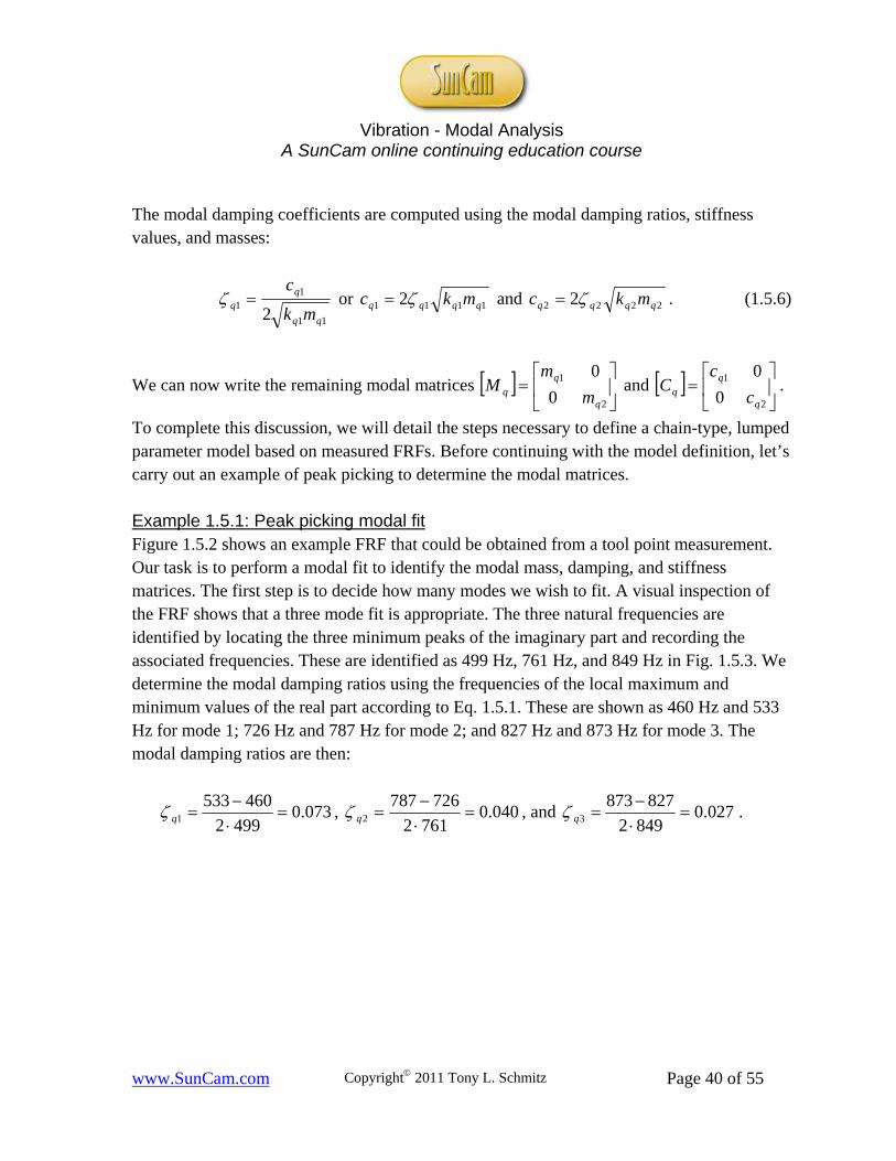
To complete this discussion, we will detail the steps necessary to define a chain-type, lumped parameter model based on measured FRFs. Before continuing with the model definition, let’s carry out an example of peak picking to determine the modal matrices. Example 1.5.1: Peak picking modal fit Figure 1.5.2 shows an example FRF that could be obtained from a tool point measurement. Our task is to perform a modal fit to identify the modal mass, damping, and stiffness matrices. The first step is to decide how many modes we wish to fit. A visual inspection of the FRF shows that a three mode fit is appropriate. The three natural frequencies are identified by locating the three minimum peaks of the imaginary part and recording the associated frequencies. These are identified as 499 Hz, 761 Hz, and 849 Hz in Fig. 1.5.3. We determine the modal damping ratios using the frequencies of the local maximum and minimum values of the real part according to Eq. 1.5.1. These are shown as 460 Hz and 533 Hz for mode 1; 726 Hz and 787 Hz for mode 2; and 827 Hz and 873 Hz for mode 3. The modal damping ratios are then:

073.04992

4605331

q , 040.07612

7267872

q , and 027.08492

8278733

q .




0 500 1000 1500

-2

0

2x 10

-6

Re

al (

m/N

)

0 500 1000 1500

-4

-2

0x 10

-6

Frequency (Hz)

Ima

g (

m/N

)

Figure 1.5.2: Example tool point FRF for peak picking exercise.

0 500 1000 1500

-2

0

2x 10

-6

Re

al (

m/N

)

0 500 1000 1500

-4

-2

0x 10

-6

Frequency (Hz)

Ima

g (

m/N

)

460 Hz

533787

827

726

849

827

849

499 Hz-7.62x10-6 m/N

849 Hz-3.72x10-6

761 Hz-2.77x10-6

Figure 1.5.3: Three degree of freedom peak picking example with required frequencies and amplitudes identified.




The imaginary part negative peak values for each mode are also listed in Fig. 1.5.3. The modal stiffness values are calculated using Eq. 1.5.3.

6

71 1099.81062.7073.02

1

qk N/m

6

62 1051.41077.2040.02

1

qk N/m

6

63 1098.41072.3027.02

1

qk N/m

We find the modal masses using Eq. 1.5.5. We must be sure to pay special attention to units for these calculations; note that we have switched from frequency units of Hz to rad/s by

multiplying by 2 and the stiffness values are expressed in N/m.

914.0

2499

1099.82

6

1

qm kg

197.0

2761

1051.42

6

2

qm kg

175.0

2849

1098.42

6

3

qm kg

Finally, the modal damping coefficients are determined using Eq. 1.5.6. Again, units compatibility should be ensured. In the following calculations, stiffness and mass values are expressed in N/m and kg, respectively, to obtain damping coefficient units of N-s/m.

419914.01099.8073.02 61 qc N-s/m

4.75197.01051.4040.02 62 qc N-s/m

4.50175.01098.4027.02 63 qc N-s/m

The 3x3 modal matrices can now be written as:

175.000

0197.00

00914.0

qM kg,

4.5000

04.750

00419

qC N-s/m, and




6

6

6

1098.400

01051.40

001099.8

qK N/m.

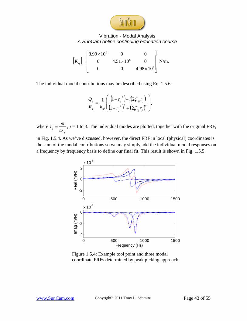
The individual modal contributions may be described using Eq. 1.5.6:

222

2

21

211

jqjj

jqjj

qjj

j

rr

rir

kR

Q

,

where nj

jr

, j = 1 to 3. The individual modes are plotted, together with the original FRF,

in Fig. 1.5.4. As we’ve discussed, however, the direct FRF in local (physical) coordinates is the sum of the modal contributions so we may simply add the individual modal responses on a frequency by frequency basis to define our final fit. This result is shown in Fig. 1.5.5.

0 500 1000 1500

-2

0

2x 10

-6

Re

al (

m/N

)

0 500 1000 1500

-4

-2

0x 10

-6

Frequency (Hz)

Ima

g (

m/N

)

Figure 1.5.4: Example tool point and three modal coordinate FRFs determined by peak picking approach.




For this contrived example, the original modal parameters used to construct the “measured” FRF are known. Therefore, we can compare our modal approximation to the true values. These results are provided in Table 1.5.1. Table 1.5.1: True modal parameters and values obtained by peak picking modal fit.

Mode 1 Mode 2 Mode 3 True Fit True Fit True Fit

fn (Hz) 500 499 760 761 850 849

q 0.090 0.073 0.050 0.040 0.030 0.027

kq (N/m) 61000.8 61099.8 61000.4 61051.4 61000.5 61098.4

Model definition Once we have determined the modal matrices by peak picking, the next step in defining a model is to use the measured direct and cross FRFs to find the mode shapes and construct the modal matrix. We’ll again assume that the measured direct FRF, shown in Fig. 1.5.1, can be approximated with a two mode fit. This means that our model will have two degrees of freedom. As we’ve seen, for a two degree of freedom model, the mode shapes are 2x1 vectors so that the square modal matrix has dimensions of 2x2. Because the mode shapes have just two entries (one of which is 1), we only require one cross FRF to determine the second entry. As before, we can choose the coordinate to which we normalize our mode

shapes for the model shown in Fig. 1.4.1. Let’s define the coordinate of interest as 2x so that

the form of the modal matrix is

1121 pp

P . We determine 1p and 2p using: 1) the

peak imaginary part values denoted C, corresponding to the first mode with the natural

frequency 1n , and D, the second mode with the natural frequency 2n , in the cross FRF2

shown in Fig. 1.5.6, together with: 2) the A and B values identified in Fig. 1.5.1.

2 We observe that the cross FRF in Fig. 1.5.6 looks very different than the direct FRF in Fig. 1.5.1; the higher frequency mode is “upside down” in Fig. 1.5.6. As we saw in Section 1.4, this is because the two modes are out of phase for the cross FRF, which results in the sign change.




1

11

11

1

2

1

2p

k

k

p

A

C

qq

qq

and 2

22

22

2

2

1

2p

k

k

p

B

D

qq

qq

(1.5.7)

We have used the ratio of the peak of the cross FRF to the direct FRF in each mode to determine the mode shapes because, as we discussed previously, the cross FRF can be expressed as the sum of the modal contributions with each mode scaled by the corresponding system mode shape. See Eq. 1.4.7. Once we have defined the modal matrix, we can determine the model parameters in local coordinates using the transformations (from modal

to local coordinates) in Eqs. 1.5.8-1.5.10. The forms of M , C , and K correspond to the

pre-selected two degree of freedom chain-type, lumped parameter model.

2

11

0

0

m

mMPMP q

T (1.5.8)

0 500 1000 1500

-2

0

2x 10

-6

Re

al (

m/N

)

0 500 1000 1500

-4

-2

0x 10

-6

Frequency (Hz)

Ima

g (

m/N

)

Figure 1.5.5: Example tool point FRF with three degree of freedom modal fit obtained by peak picking.




22

2211

cc

cccCPCP q

T (1.5.9)

22

2211

kk

kkkKPKP q

T (1.5.10)

As a final note regarding model definition, it should be emphasized that if the measured direct FRF has three modes that we wish to model, then the square modal matrix will have dimensions of 3x3. To determine the modal matrix, we must measure, at minimum, two cross FRFs to give the two ratios required for the 3x1 mode shapes. Additional cross FRF measurements may be necessary to find measurement locations with good signal to noise ratio (i.e., away from system nodes, or locations of zero vibration amplitude regardless of the force input level). Modal truncation Prior to describing modal testing equipment, there is one remaining issue to highlight regarding modal fitting. Because FRF measurements always have a finite frequency range and elastic bodies possess an infinite number of degrees of freedom, there are necessarily

Re

al

Frequency (Hz)

Ima

g

D

C

Figure 1.5.6: Two degree of freedom cross FRF with the amplitudes required for model development identified.




modes that exist outside the measurement range. We typically measure from zero to a few of kHz at most (perhaps up to 10 kHz for a small mass impact hammer with a steel tip – see Section 1.6). However, omitting these higher frequency modes during peak picking affects the accuracy of the modal fit, particularly the real part of the FRF. Equations 1.2.6 and 1.2.7, which describe the real and imaginary parts of a single degree of freedom FRF, are reproduced here to demonstrate the effect.

222

2

21

11Re

rr

r

kF

X

(1.5.11)

222 21

21Im

rr

r

kF

X

(1.5.12)

It is seen that when the frequency ratio n

r

is large, or the driving frequency is very

high and outside the measurement range, the denominator within the right parenthetical terms in these two equations becomes very large and the response approaches zero. This is seen at the right hand side of Fig. 1.2.4, for example. However, as r approaches zero, the parenthetical term in the real part approaches one and the parenthetical term in the imaginary

part approaches zero. Therefore, the value of the real part approaches k

1 as r approaches

zero3. If there are modes beyond the measurement bandwidth, neglecting these terms and the

associated k

1 contributions leads to errors in the vertical location of the modal fit’s real part.

This is demonstrated in Ex. 1.5.2. Example 1.5.2: High frequency mode truncation during modal fitting A “measured” FRF is provided in Fig. 1.5.7. We will presume that the measurement bandwidth was 2 kHz, although a 5 kHz frequency range is shown for demonstration purposes. Within the 2 kHz range, two modes are visible and peak picking can be applied to determine the associated modal parameters. Using the values from the figure, the modal stiffness, mass, and damping matrix terms may be determined as shown in Ex. 1.5.1.

3 This

k

1 term can be referred to as the DC compliance.




049.03752

3563931

q 020.011002

107811222

q

7

71 1050.11074.6049.02

1

qk N/m

6

62 1099.31026.6020.02

1

qk N/m

70.2

2375

1050.12

7

1

qm kg

084.0

21100

1099.32

6

2

qm kg

62470.21050.1049.02 71 qc N-s/m

2.23084.01099.3020.02 62 qc N-s/m

The fit to the measured direct FRF is determined by summing the two contributions in modal coordinates according to:

0 1000 2000 3000 4000 5000

-2

0

2

4x 10

-6

Re

al (

m/N

)

0 1000 2000 3000 4000 5000

-6

-4

-2

0x 10

-6

Frequency (Hz)

Ima

g (

m/N

)

356 Hz

393

1078

1122

375-6.74x10-7 1100 Hz

-6.26x10-6 m/N

Figure 1.5.7: “Measured” direct FRF for Ex. 1.5.2. The peak picking values are listed within the 2 kHz measurement bandwidth. A 5 kHz frequency range is provided to show the truncated 4000 Hz mode.




222

222

222

2

22

11

221

112

1

12

2

1

1

21

211

21

211

rr

rir

krr

rir

kR

Q

R

Q

F

X

q

q

qq

q

q

,

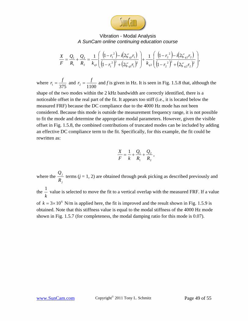
where 3751

fr and

11002

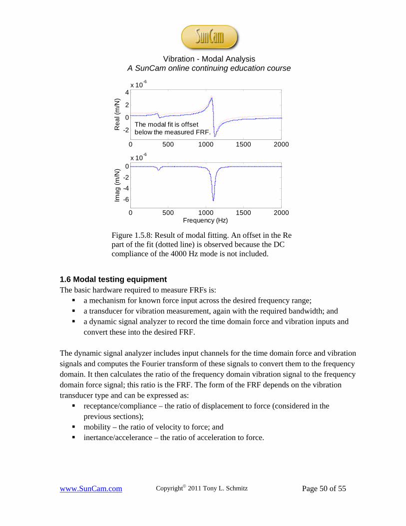
fr and f is given in Hz. It is seen in Fig. 1.5.8 that, although the

shape of the two modes within the 2 kHz bandwidth are correctly identified, there is a noticeable offset in the real part of the fit. It appears too stiff (i.e., it is located below the measured FRF) because the DC compliance due to the 4000 Hz mode has not been considered. Because this mode is outside the measurement frequency range, it is not possible to fit the mode and determine the appropriate modal parameters. However, given the visible offset in Fig. 1.5.8, the combined contributions of truncated modes can be included by adding an effective DC compliance term to the fit. Specifically, for this example, the fit could be rewritten as:

2

2

1

11

R

Q

R

Q

kF

X ,

where the j

j

R

Q terms (j = 1, 2) are obtained through peak picking as described previously and

the k

1 value is selected to move the fit to a vertical overlap with the measured FRF. If a value

of 6103k N/m is applied here, the fit is improved and the result shown in Fig. 1.5.9 is obtained. Note that this stiffness value is equal to the modal stiffness of the 4000 Hz mode shown in Fig. 1.5.7 (for completeness, the modal damping ratio for this mode is 0.07).




1.6 Modal testing equipment The basic hardware required to measure FRFs is: a mechanism for known force input across the desired frequency range; a transducer for vibration measurement, again with the required bandwidth; and a dynamic signal analyzer to record the time domain force and vibration inputs and

convert these into the desired FRF. The dynamic signal analyzer includes input channels for the time domain force and vibration signals and computes the Fourier transform of these signals to convert them to the frequency domain. It then calculates the ratio of the frequency domain vibration signal to the frequency domain force signal; this ratio is the FRF. The form of the FRF depends on the vibration transducer type and can be expressed as: receptance/compliance – the ratio of displacement to force (considered in the

previous sections); mobility – the ratio of velocity to force; and inertance/accelerance – the ratio of acceleration to force.

0 500 1000 1500 2000

-2

0

2

4x 10

-6

Re

al (

m/N

)

0 500 1000 1500 2000

-6

-4

-2

0x 10

-6

Frequency (Hz)

Ima

g (

m/N

)The modal fit is offsetbelow the measured FRF.

Figure 1.5.8: Result of modal fitting. An offset in the Re part of the fit (dotted line) is observed because the DC compliance of the 4000 Hz mode is not included.




Force input Common types of force excitation include: fixed frequency sine wave – The complex response is determined one frequency at a

time with averaging occurring at each frequency over a short time interval. This is referred to as a sine sweep test.

random signal – The frequency content of the random signal may be broadband (white noise) or truncated to a desired range (pink noise). Averaging over a fixed period of time is again applied.

impulse – A short duration impact is used to excite the structure. This approach enables a broad range of frequencies to be excited in a single, short test. Multiple tests are typically averaged in the frequency domain to improve coherence, or the correlation between the force and vibration signals.

Common force input hardware includes: shaker – These systems include a harmonically driven armature and a base. The

armature may be actuated along its axis by a magnetic coil or hydraulic force. The magnetic coil, or electrodynamic, configurations can provide excitation frequencies of tens of kHz with force levels from tens to thousands of N (increased force typically means a lower frequency range). Hydraulic shakers offer high force with the potential

0 500 1000 1500 2000

-2

0

2

4x 10

-6

Re

al (

m/N

)

0 500 1000 1500 2000

-6

-4

-2

0x 10

-6

Frequency (Hz)

Ima

g (

m/N

)

Figure 1.5.9: Result of modal fitting with the addition of a DC compliance term to correct for the truncated mode.




for a static preload, but relatively lower frequency ranges. In either case, the force is often applied to the structure of interest through a “stinger”, or a slender rod that supports axial tension and compression, but not bending or shear. A load cell is often incorporated in the setup to measure the input force. One consideration is that this load cell adds mass to the system under test, which can alter the FRF for low mass structures. Finally, the shaker must be isolated from the structure to prevent reaction forces due to the shaker motion from being transmitted through the shaker base to the structure. See Fig. 1.6.1.

Figure 1.6.1: Shaker example. The stinger is shown extending from the top end [7].




impact hammer – An impact hammer incorporates a force transducer in a metal, plastic, or rubber tip to measure the force input during a hammer strike. Because the setup and measurement time is short, it is a popular choice for tool-holder testing (referred to as impact testing). Naturally, the energy input to the structure is a function of the hammer mass; therefore, many sizes are available. Also, the bandwidth of the force input depends on the mass and tip stiffness. Stiffer tips tend to excite a wider frequency range, but also spread the input energy over this wider range. Softer tips concentrate the energy over a lower frequency range. Hard, plastic tips are a common choice for tool testing because they do not damage the cutting edge and generally provide sufficient excitation bandwidth. See Fig. 1.6.2.

Figure 1.6.2: Example impact hammer. Many sizes and tip types are available. A medium sized hammer (0.32 kg) is shown [8].




Vibration measurement Vibration transducers are available in both non-contact and contact types. While non-contact transducers, such as capacitance probes and laser vibrometers, are preferred because they do not influence the system dynamics, contacting types, such as accelerometers, are more convenient to implement. As a compromise, low mass accelerometers are often used. See Fig. 1.6.3. In most applications, the addition of a few grams or less of accelerometer mass does not appreciably alter the response and the accelerometer can be attached using wax and then easily removed. Because accelerometers produce a signal which is proportional to

acceleration, the inertance FRF is obtained. However, to convert from inertance, or F

A, to

receptance, F

X, we can use the relationship:

F

A

F

X

2

1

, (1.6.1)

which follows from the harmonic solution, tiXex , and its second time derivative

xXex ti 22 . Equation 1.6.1 effectively describes double numerical integration in the frequency domain.

Figure 1.6.3: Example accelerometer with 10 mg mass and 0.5 Hz to 5 kHz measurement bandwidth. Many sizes are available for various applications [9].




References 1. http://en.wikipedia.org/wiki/Modal_analysis, accessed July, 2008. 2. http://en.wikipedia.org/wiki/Tacoma_Narrows_Bridge, accessed July, 2008. 3. Inman, D., 2001, Engineering Vibration, 2nd Ed., Prentice Hall, Upper Saddle River, NJ,

Section 1.10. 4. Thomson, W. and Dahleh, M., 1998, Theory of Vibration with Application, 5th Ed.,

Prentice Hall, Upper Saddle River, NJ, Section 3.9. 5. Leon, J., 1994, Linear Algebra with Applications, 4th Ed., Prentice Hall, Englewood

Cliffs, NJ, Section 5.6. 6. Ewins, D., 2000, Modal Testing: Theory, Practice, and Application, 2nd Ed., Taylor &

Francis, London. 7. http://www.modalshop.com/test_tmproducts.asp?ID=164, accessed July, 2008. 8. http://www.pcb.com/spec_sheet.asp?model=086D05&item_id=10517, accessed July,

2008. 9. http://www.pcb.com/spec_sheet.asp?model=338C24&item_id=2009, accessed July,

2008.

Documents

A SunCam online continuing education course Vibration - Modal … · 2017-01-11 · A SunCam online continuing education course Vibration - Modal Analysis by ... everyday object has