The Pennsylvania State University

The Graduate School

College of Engineering

A STUDY ON THE SOOTING TENDENCY OF JET FUEL

SURROGATES USING THE THRESHOLD SOOT INDEX

A Thesis in

Mechanical Engineering

by

Amy Mensch

© 2009 Amy Mensch

Submitted in Partial Fulfillment

of the Requirements

for the Degree of

Master of Science

May 2009

ii

The thesis of Amy Mensch was reviewed and approved* by the following:

Robert J. Santoro

George L. Guillet Professor of Mechanical Engineering

Thesis Co-Adviser

Thomas A. Litzinger

Professor of Mechanical Engineering

Thesis Co-Advisor

Stephen R. Turns

Professor of Mechanical Engineering

Karen A. Thole

Professor of Mechanical Engineering

Head of the Department of Mechanical and Nuclear Engineering

*Signatures are on file in the Graduate School.

iii

ABSTRACT

Currently, modeling the combustion of aviation turbine fuels is not feasible due to

the complexity and variation of real fuels. Surrogates, created out of a few pure

hydrocarbon compounds, are a key step toward modeling new engines and new fuels.

For the surrogate to simulate the real fuel, the composition must be designed to reproduce

certain pre-designated parameters. In the present research, instead of attempting to match

distillation curves or estimates of the composition of the real fuel, three combustion

related parameters including hydrogen to carbon (H/C) ratio, cetane number, and sooting

tendency are to be reproduced. The objective of this thesis is to characterize the sooting

tendency. The tendency of a fuel to produce soot in the combustor is relevant because it

affects flame radiation as well as emissions. Parameters which characterize sooting

tendency include hydrogen content, H/C ratio, smoke point, Threshold Soot Index (TSI),

Yield Sooting Index (YSI), and others. In this work, TSI, which is derived from the

smoke point measurement, is used.

Previous data on TSI had been scaled inconsistently, and widely differing values

for some compounds had been reported. In addition, the TSI for a key iso-alkane, iso-

cetane, had not been measured. Therefore this work sought to provide a complete and

consistent set of TSI values for surrogate components. Smoke point heights of sixteen

compounds were measured according to ASTM D1322, and TSI values were derived

from these measurements. The soot threshold and soot yield (YSI) data from prior

studies were rescaled with a correlation to the TSI values from the current study. The

magnitude of the correlation coefficient was used to determine whether the data set was

used in the final average TSI values. Results showed that the differences in TSI values

were significantly reduced by scaling all the data sets in this manner.

Once individual TSI values are known, the resulting TSI when components are

mixed together can be predicted. Previous researchers tested a mixture rule, which was

iv

shown to hold for the mixtures investigated. In this work, it was found that six additional

binary mixtures and four multi-component mixtures follow the same mixture rule. A

method of calculating the TSI of a single component from the mixture TSI was used to

obtain a TSI value for iso-cetane, which could not otherwise be measured, and to verify

the TSI value for 1-methylnaphthalene.

Due to the complex molecular structures of aromatics, it is one of the hydrocarbon

classes for which developing chemical kinetic models is difficult. Among the

hydrocarbon families, aromatics also have the highest sooting tendencies, and their

presence has the most effect on TSI. Due to inadequate development of some chemical

kinetic models, certain aromatic compounds may need to be replaced with others for

which models exist. The TSI values of three mixtures were tested to show that TSI can

be replicated using different combinations of compounds for the aromatic fraction of the

mixture.

The methodology of designing surrogates based on TSI was applied to JP-8, the

USAF jet fuel. The smoke point height of JP-8 was measured, and the TSI was obtained

using an estimated molecular weight. A surrogate, created to match the JP-8 TSI,

produced the same value within the estimated uncertainty. The formation of a set of TSI

values for individual compounds and the verification of a mixture rule showed that TSI

can be used as a sooting tendency parameter for designing surrogate composition.

v

TABLE OF CONTENTS

NOMENCLATURE ......................................................................................................... vii

LIST OF FIGURES ......................................................................................................... viii

LIST OF TABLES .............................................................................................................. x

ACKNOWLEDGEMENTS ............................................................................................... xi

CHAPTER 1 INTRODUCTION ........................................................................................ 1

1.1 Motivation and Background ............................................................................. 1

1.2 Objectives of the Research ................................................................................ 4

CHAPTER 2 LITERATURE REVIEW ............................................................................. 5

2.1 Background on Jet Fuels ................................................................................... 5

2.2 Soot Threshold or Smoke Point ........................................................................ 6

2.3 Threshold Soot Index, TSI .............................................................................. 10

2.4 Yield Sooting Index, YSI ................................................................................ 14

2.5 TSI for Mixtures ............................................................................................. 16

2.6 Correlations of Soot Measurements with TSI ................................................. 17

2.7 Summary of Soot Threshold as a Measure of Sooting Tendency ................... 18

CHAPTER 3 EXPERIMENTAL APPROACH ............................................................... 19

3.1 Experimental Apparatus.................................................................................. 19

3.2 Experimental Procedure .................................................................................. 20

3.3 Mixture Preparation ........................................................................................ 29

3.4 Procedure for TSI Calculation ........................................................................ 30

3.5 Uncertainty Analysis ....................................................................................... 31

CHAPTER 4 RESULTS AND DISCUSSION ................................................................. 34

vi

4.1 TSI for Pure Compounds ................................................................................ 34

4.3 Achieving Matching TSI Values with Different Compounds ........................ 49

4.4 Matching the TSI of JP-8 with a Surrogate .................................................... 51

CHAPTER 5 CONCLUSIONS ........................................................................................ 54

CHAPTER 6 FUTURE WORK ....................................................................................... 56

REFERENCES ................................................................................................................. 57

Appendix A. SP, ambient conditions, and TSI for Standard Mixtures ............................. 59

Appendix B. SP and TSI Data for Binary Mixtures ......................................................... 61

vii

NOMENCLATURE

a, b = apparatus specific Threshold Soot Index constants

c, d = apparatus specific Yield Sooting Index constants

fv,max = the maximum soot volume fraction

i-cet = iso-cetane

K = smoking tendency constant

m = fuel mass flowrate

MCH = methylcyclohexane

1-MN = 1-methylnaphthalene

MW = molecular weight

SP = height of the flame at the smoke point

St = smoking tendency

TMB = trimethylbenzene

TSI = Threshold Soot Index

YSI = Yield Sooting Index

viii

LIST OF FIGURES

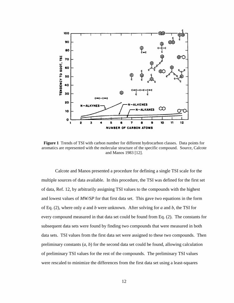
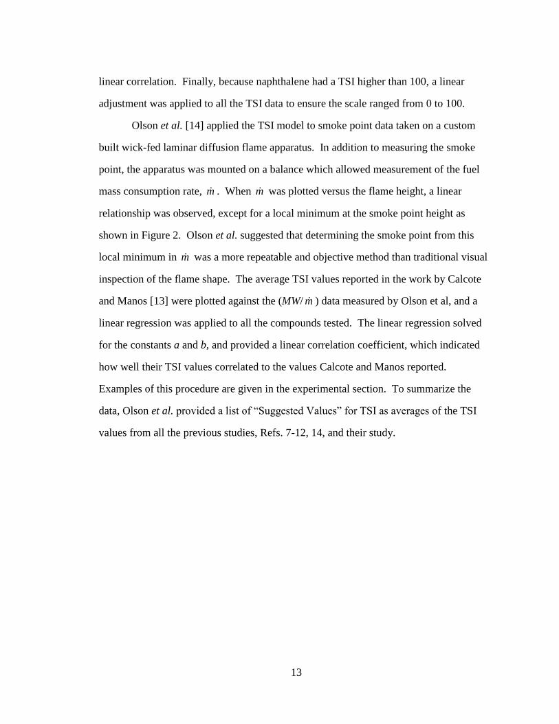
Figure 1 Trends of TSI with carbon number for different hydrocarbon classes. Data

points for aromatics are represented with the molecular structure of the specific compound.

Source, Calcote and Manos 1983 [12]. ............................................................................. 12

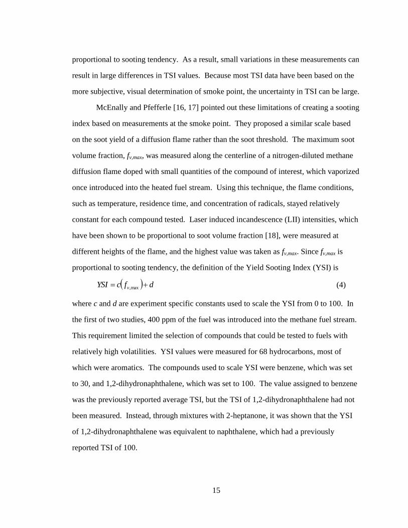
Figure 2 Relationship between flame height and fuel mass consumption rate of n-

propylbenzene and 1-octene. Arrows point to local minimum observed at the smoke

point. Source, Olson et al. 1985 [13]. .............................................................................. 14

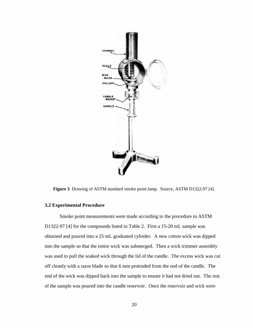
Figure 3 Drawing of ASTM standard smoke point lamp. Source, ASTM D1322-97 [4].

........................................................................................................................................... 20

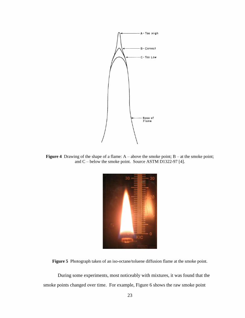
Figure 4 Drawing of the shape of a flame: A – above the smoke point; B – at the smoke

point; and C – below the smoke point. Source ASTM D1322-97 [4]. ............................ 23

Figure 5 Photograph taken of an iso-octane/toluene diffusion flame at the smoke point.

........................................................................................................................................... 23

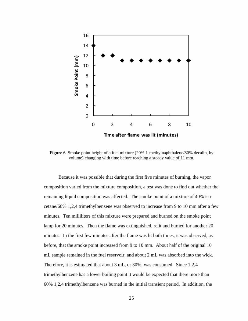
Figure 6 Smoke point height of a fuel mixture (20% 1-methylnaphthalene/80% decalin,

by volume) changing with time before reaching a steady value of 11 mm. ..................... 25

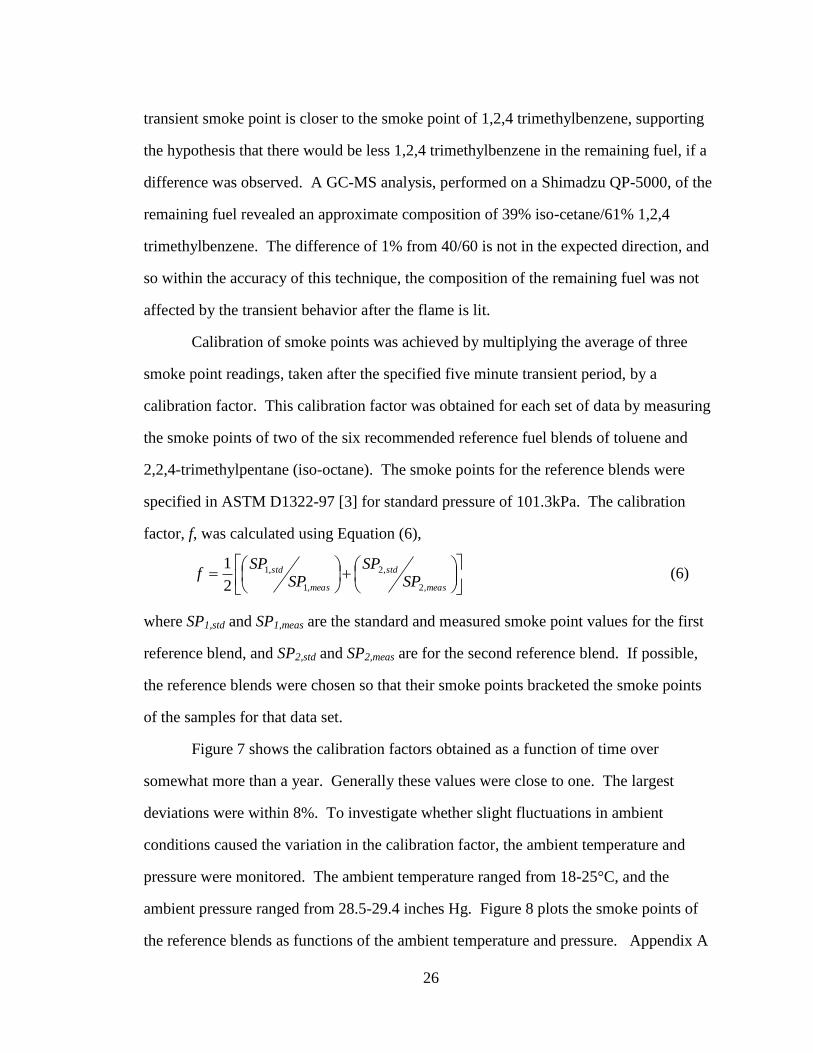
Figure 7 Calibration factor, f, plotted as a function of time. ........................................... 27

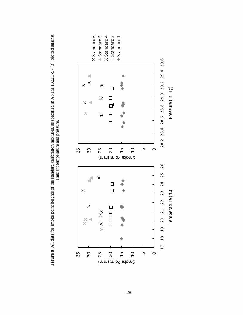
Figure 8 All data for smoke point heights of the standard calibration mixtures, as

specified in ASTM 1322D-97 [3], plotted against ambient temperature and pressure. ... 28

Figure 9 Scaling of TSI data. TSI values obtained in this work plotted against MW/SP

data from Minchin, 1931 [7] and Clarke et al., 1946 [8]. Linear fit defines TSI for a

given MW/SP from those studies. ..................................................................................... 37

ix

Figure 10 Scaling of TSI data. TSI values obtained in this work plotted against MW/SP

data from Hunt, 1953 [12] and Gill and Olson, 1984 [19]. Linear fit defines TSI for a

given MW/SP from those studies. ..................................................................................... 38

Figure 11 Scaling of TSI data. TSI values obtained in this work plotted against MW/ m

data from Schalla and McDonald, 1953 [11] and Olson et al., 1985 [14]. Linear fit

defines TSI for a given MW/ m from those studies. ......................................................... 39

Figure 12 Scaling of TSI data. TSI values obtained in this work plotted against YSI

from McEnally and Pfefferle, 2007 [16] and 2008 [17]. Linear fit defines TSI for a

given YSI from those studies. ........................................................................................... 40

Figure 13 Variation of TSI with mole fraction for three binary mixtures. Points are

measured TSI values, and lines are TSI values calculated from pure component values.

To differentiate between the error bars, those for calculated TSI values are represented as

dashed lines and are offset by 0.01 in mole fraction......................................................... 45

Figure 14 Variation of TSI with mole fraction for three binary mixtures containing 1-

methylnaphthalene (1-MN). Points are measured TSI values, and lines are TSI values

calculated from pure component values. To differentiate between the error bars, those for

calculated TSI values are represented as dashed lines and are offset by 0.01 in mole

fraction. ............................................................................................................................. 46

Figure 15 Binary mixtures containing 1-methylnaphthalene, used to calculate the TSI

for pure 1-methylnaphthalene from the fit lines. .............................................................. 49

x

LIST OF TABLES

Table 1 Minimum, maximum, and average properties values of JP-8, from the 2006

PQIS report [5]. ................................................................................................................... 6

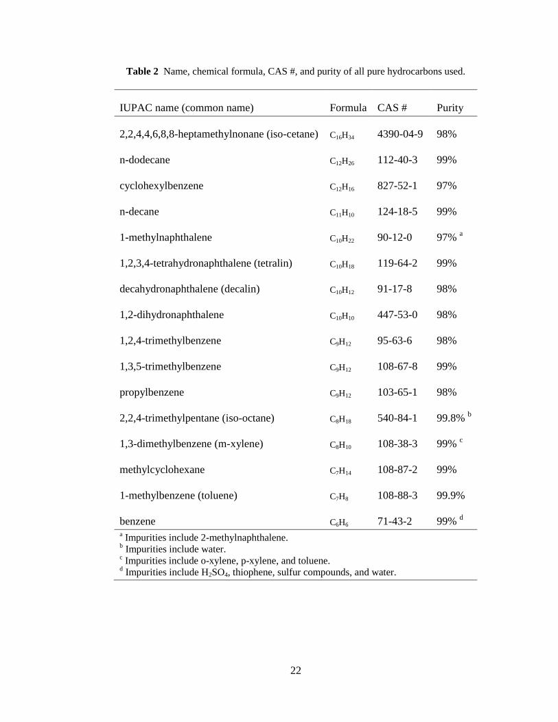
Table 2 Name, chemical formula, CAS #, and purity of all pure hydrocarbons used. ... 22

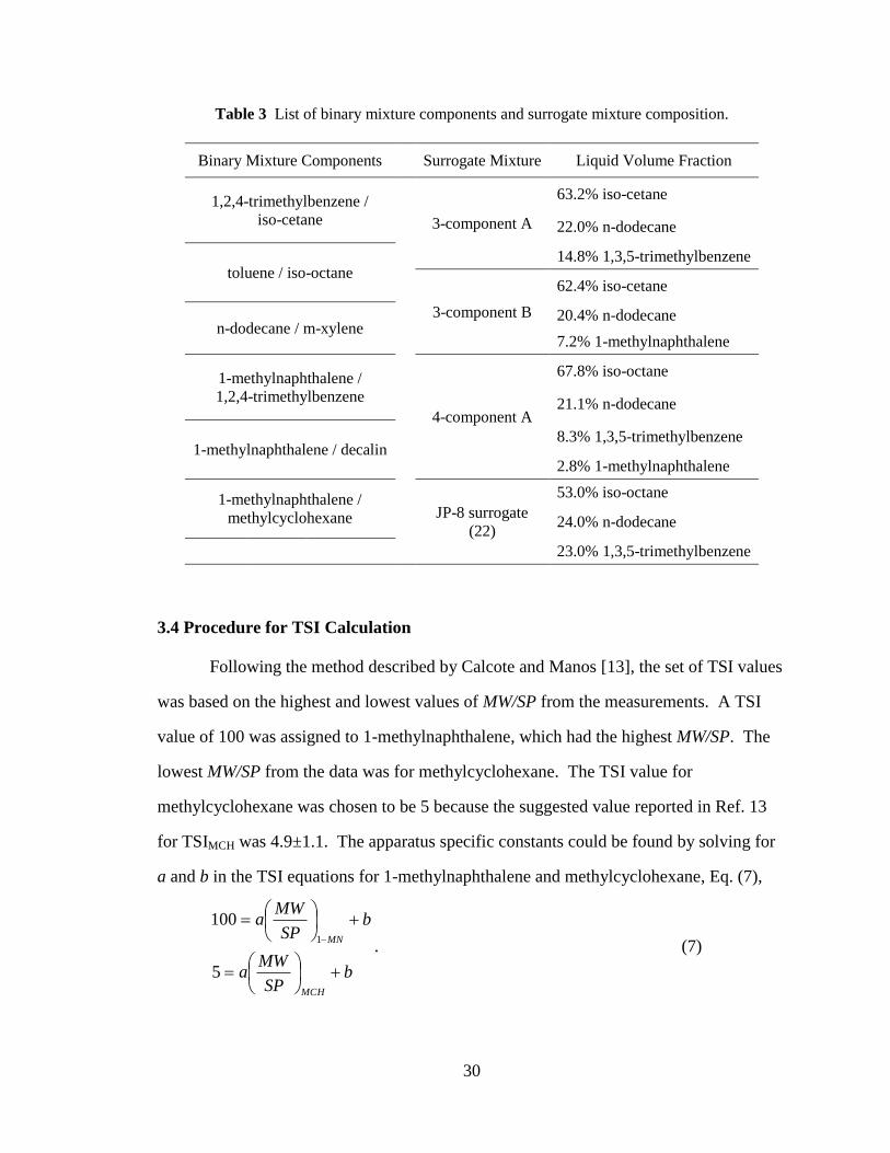
Table 3 List of binary mixture components and surrogate mixture composition. .......... 30

Table 4 Smoke point height, TSI, and relative uncertainty in TSI for pure compounds. 34

Table 5 Sources of sooting threshold data for pure hydrocarbons, which measured two

or more compounds in common with this work. .............................................................. 36

Table 6 TSI values for compounds considered in this work. Data include TSI values

measured in this study, rescaleda TSI values from studies with R

2 > 0.95, Schalla and

McDonald [11], Olson et al. [14], Gill and Olson [19], and McEnally and Pfefferle [16,

17], and an average of these TSI values. .......................................................................... 42

Table 7 Composition, smoke point height, measured TSI, and predicted TSI of three

MURI [2] surrogate mixtures for JP-8. ............................................................................. 51

Table 8 Smoke point height and TSI results for JP-8 samples taken from the same batch

of fuel. ............................................................................................................................... 52

Table 9 Composition, smoke point height, measured TSI, and predicted TSI for a

surrogate matching JP-8 in TSI and H/C ratio. ................................................................. 53

xi

ACKNOWLEDGEMENTS

I would like to sincerely thank my advisor, Prof. Robert Santoro, for his support

and encouragement. The knowledge and experience I have gained as a result of this

opportunity to work with him is indispensable. Throughout the progression of this

research, I was treated with respect and understanding. I greatly appreciate the guidance

of Prof. Thomas Litzinger as my co-advisor, who has helped me with research and

communication skills. I extend thanks to Prof. Stephen Turns for reviewing this thesis.

I am grateful for the feedback and suggestions from the attendees of the weekly

soot meetings: Venkatesh Iyer, Dr. Suresh Iyer, Dr. Milton Linevsky, and especially Dr.

Seong-Young Lee and Arvind Menon for their general support with experiment and

technology issues as well. I would also like to acknowledge Dr. Yi Yang for his help

with the smoke point measurements. I would like to express thanks to the Department of

Mechanical and Nuclear Engineering as well.

I would like to acknowledge the financial support of the Air Force Office of

Scientific Research under the MURI – Generation of Comprehensive Surrogate Kinetic

Models and Validation Databases for Simulating Large Molecular Weight Hydrocarbon

Fuels. I would like to thank the contract monitor, Dr. Julian Tishkoff, and the Principle

Investigator, Prof. Frederick Dryer, for their guidance and support of this work. I also

thank Dr. Meredith Colket and Prof. Charles McEnally for their helpful discussions on

TSI and YSI.

I am very grateful to my family, including my parents, grandparents, and aunts

and uncles, who have all supported and advised me. Without them I would have not

made it to this point.

1

CHAPTER 1 INTRODUCTION

1.1 Motivation and Background

Combustion modeling is necessary for the development of efficient and accurate

numerical design methodologies for engines. By modeling proposed changes to engine

designs ahead of time, the number of costly and time consuming engine tests can be

reduced. As the desire grows to employ alternative liquid fuels, energy sources such as

coal and bio-feedstocks will be used. Often the alternative fuels from these sources have

significantly different chemical or physical properties than the original petroleum based

fuel. Modeling the combustion of the alternative fuels will become important to predict

any effects on engine performance and emissions.

The concept of surrogate fuels developed from a need to model the combustion of

practical liquid fuels used in existing and future engine designs. A surrogate fuel is a

mixture of a small number of pure compounds that can mimic the combustion of a real

fuel, whether it is derived from petroleum or an alternative source. Practical fuels are

often composed of thousands of components, which can vary with location and time of

year [1]. The variation is acceptable because specifications generally require fuels to

meet certain values on empirical tests, but do not specify composition. The resulting

multi-component and variable nature of practical fuels introduces overwhelming

complexity to the modeling task. A surrogate fuel requires a much simpler chemical

kinetic model than would be needed for the practical fuel. Therefore, with surrogate fuels

to represent the real fuel, designing engines and developing new fuels using modeling

becomes possible.

The work to be discussed is part of a Multi-disciplinary University Research

Initiative (MURI) [2] to develop surrogate fuel mixtures of three to five components and

related kinetic models for the United States Air Force jet fuel, JP-8. In automobile

2

engines, the technique of substituting surrogates for practical fuels has been used

successfully to model the combustion of gasoline. However, developing functioning

surrogates for aviation jet fuels is more difficult for several reasons. Jet fuel has a higher

average molecular weight than gasoline, which means chemical kinetic models of the

individual mixture components of a jet fuel surrogate are harder to develop. Also, the

specifications for jet fuels are relatively broad and include fuels with a rather wide range

of properties, implying composition can vary significantly [2].

To be useful the surrogate fuel must match key combustion processes with

reasonable fidelity, and models must be carefully constructed, which presents some

challenges. Rules for selecting surrogate components and matching mixtures against real

jet fuels have not been previously defined. One of the goals of the MURI is to develop a

methodology for designing surrogates that can be applied to any fuel. It is proposed that

a surrogate must meet a few important combustion-related parameters to be considered.

In addition, there is a lack of kinetic model validation data for higher molecular weight

compounds and their mixtures.

The MURI has identified three combustion-related parameters as crucial

parameters to be reproduced by the surrogate: hydrogen to carbon (H/C) ratio,

autoignition characteristics, and sooting tendency [2]. The H/C ratio has been shown to

be important for many combustion quantities, such as heat of reaction, flame temperature,

flame speed, and local air-to-fuel ratio. The work here focuses on the development and

use of the parameter for sooting tendency. The surrogate fuel should be able to

accurately simulate in-combustor soot formation as well as soot emissions of JP-8. The

sooting characteristics of JP-8 are important because radiation from soot formed in the

combustor heats and stresses the combustor liner. Soot particles that escape from the

combustor deposit in the turbine section or leave with the exhaust as soot emissions.

Studies of sooting tendency of hydrocarbon fuels have been done in a number of

combustors and burners. A simple diffusion flame has been especially useful, as it is a

3

key element of the United States Air Force (USAF) specifications for jet fuel with respect

to soot. In diffusion flames, the threshold of soot breakthrough is identified as the

condition at which soot particles are observed to exit the flame, and is commonly referred

to as the smoke point (SP). Measurements show that the smoke point occurs at different

flame heights for different fuels. Thus, the smoke point has been used as an important

predictor of soot formation for years. The Threshold Soot Index (TSI), which is a linear

function of the molecular weight of the fuel divided by the smoke point defined in Eq.

(2), can be used as a measure of sooting tendency for fuels for which these quantities are

known [13]. Some parameters that have been used to characterize sooting tendency of

fuels include hydrogen content, H/C ratio, smoke point, TSI, and Yield Sooting Index

(YSI) [16, 17]. TSI has been chosen to be the sooting tendency parameter for this effort

because of its consistency and relationship to the smoke point measurement. The critical

parameters for the MURI methodology, such as TSI, can match those of the practical fuel

by varying the composition of the surrogate once the base components have been

selected.

The selection of surrogate components for the aviation jet fuel, JP-8, reflects the

type of molecular structures in the real fuel, as well as the availability of chemical kinetic

models for which validation data already exist, or are under investigation as part of the

MURI collaborative projects [2] or elsewhere. As an initial approach, the surrogate for

JP-8 is created using hydrocarbons from the three main classes of compounds present in

the fuel: n-alkanes, iso-alkanes, and aromatics. Higher carbon number n-alkanes and iso-

alkanes are selected in order to achieve the typical H/C ratio and autoignition properties

of JP-8. Aromatic compounds, which are the most influential to TSI, are chosen with

consideration of the length, location and number of alkyl branches on the benzene and

naphthalene rings.

4

1.2 Objectives of the Research

The first objective was to generate a consistent set of TSI data for all the

compounds that are being considered for formulating surrogate mixtures for the MURI.

Creating a consistent set of TSI values required measuring the TSI values for a number of

hydrocarbons. In addition to the candidate surrogate compounds, more compounds were

tested for better comparison to previous studies. Previous sooting tendency

measurements include the flame height and the fuel consumption rate at the smoke point,

as well as the volume fraction of soot, known as soot yield, in a doped methane diffusion

flame (used to derive the Yield Sooting Index). TSI data derived from all three types of

measurements were incorporated into the final set of values. A second objective was to

verify that for binary mixtures, TSI values were linearly related based on the mole

fraction of the candidate surrogate compounds. A third objective was to verify that

different hydrocarbon molecules from the same class could be used to formulate

equivalent mixtures, in terms of the TSI values, using the linear mixing rule. Confirming

mixture equivalence required testing the mixtures to verify that their measured TSI values

were the same. The mixtures contained different compounds in proportions so that the

predicted TSI values of the mixtures were equal. A final objective was to test the TSI of

a surrogate mixture that was devised to match the measured TSI of JP-8. Overall, this

research attempted to show that TSI is an effective method for sooting tendency

prediction for real jet fuels.

5

CHAPTER 2 LITERATURE REVIEW

2.1 Background on Jet Fuels

Jet propulsion fuels were developed for the turbojet engine used in military

applications after World War II. Due to the availability of gasoline, the first jet fuels

were very similar to automobile gasoline [1]. Jet fuels evolved to use more of the

kerosene fraction of the petroleum distillate for improved performance in jet engine

applications. For most of the 20th

century the primary USAF fuel was JP-4, a mixture of

the gasoline and kerosene fractions. The gasoline fraction was maintained to keep a

lower freezing point leading to improved cold temperature stability and lubricity [1].

When commercial aviation developed in the 1960’s a purely kerosene fuel named Jet A

was developed. An advantage of Jet A over JP-4 was reduced flammability leading to

safer operation. The damage and losses by the USAF due to use of the highly flammable

JP-4 in the Vietnam War, motivated the switch from JP-4 to a fuel similar to Jet A [1].

The new fuel, JP-8, was practically the same as Jet A, but had an additive package to

improve lubricity and prevent accidents caused by icing and static discharge during

fueling. By 1995 the USAF completely converted to JP-8 for all aircraft and mobile

ground equipment [1].

The specifications for JP-8 were motivated by operational parameters developed

throughout the evolution of jet fuels. To specify sooting tendency, the USAF regulates

hydrogen content as well as smoke point and naphthalene content. With regard to

sooting tendency, specifications for JP-8 require the following [3]:

1. Minimum hydrogen content, 13.4% by mass

2. Minimum smoke point of 25 mm

OR

Minimum smoke point of 19 mm AND Maximum naphthalene 3% by

volume

6

The first requirement establishes the H/C ratio, which has shown some correlation with

sooting tendency in the literature. The second requirement specifies the minimum smoke

point, which is found through a standard ASTM measurement [4] of the flame height

taken at the onset of soot breakthrough of a wick-fed diffusion flame. The minimum

smoke point requirement depends on the naphthalene content, because naphthalene is

known to be a heavily sooting compound.

As described above, there is a wide range of acceptable fuels for JP-8. An

estimate of the range of properties found in JP-8 fuels is included in the 2006 Petroleum

Quality Information System (PQIS) report [5]. This report cites critical data on fuel

quality and property variations for the year. Certain chemical and physical properties

found for JP-8 are summarized in Table 1.

Table 1 Minimum, maximum, and average properties values of JP-8, from the 2006 PQIS report

[5].

Min. Max. Avg.

Hydrogen Content (mass %) 13.40 14.78 13.81

H/C Ratio 1.844 2.067 1.909

Cetane Number 31.8 56.8 43.9

Smoke Point (mm) 19.0 31.0 22.7

Aromatics (liq. vol. %) 0.10 24.60 17.86

Density (g/ml) @ 288.15 K 0.7800 0.8325 0.8038

2.2 Soot Threshold or Smoke Point

The soot threshold or smoke point is the point at which any increase in flame

height or fuel flow rate results in smoke emitted from the tip of the flame. Soot threshold

studies of diffusion flames began in the early 20th

century and continue to be relevant

today in the specifications for jet fuel. The first investigators of sooting tendency were

7

concerned with the quality of kerosene burned in oil lamps. The smoke point was

determined by observing a distinct change in the shape of the flame tip as the flame

height was adjusted. It was realized that fuels which produced more soot tended to reach

the soot threshold at lower flame heights than less sootier fuels. Kewley and Jackson [6]

studied the soot threshold on a Weber Photometer lamp, which burned liquid fuels using

a wick. The length of wick could be adjusted to find and measure the height of the

smoke point. They defined a “tendency to soot” of kerosene as the measured height

subtracted from 32 mm, the upper limit of the scale. Thus the higher the resulting value,

the higher the “tendency to soot” was for that fuel. Minchin [7], noting that in this

definition a smoke point height of 32 mm or higher would have a “tendency to soot” of

zero or below, improved the parameter to an inverse relationship,

SPKSt / , (1)

where St was called the smoking tendency, and K was an arbitrary constant. Minchin

measured the smoke point heights of seven pure hydrocarbons and three phenol

compounds using a Weber Photometer lamp. Using a correlation of the volume of the

flame, estimated roughly as a cone shape, and the required molar volume of oxygen, and

the molar volume of combustion products, Minchin predicted the smoke point heights of

compounds that had not been measured. These calculated smoke point heights allowed

Minchin to make a qualitative ranking of the sooting tendency of groups of compounds

with similar molecular structure, or hydrocarbon classes: alkanes < alkenes and mono-

cyclic cycloalkanes < di-alkenes and di-cyclic cycloalkanes < benzene series <

naphthalene series. Within each hydrocarbon class, it was found that St had a relationship

to carbon number. For paraffins, St decreased as carbon number increased, but for the

other hydrocarbon classes, St increased as carbon number increased. These observations

demonstrated that St was closely related to molecular structure.

Two other studies on smoke point were conducted on conical pool burners.

Instead of burning from a wick, the flame burned from the surface of a pool of the liquid

8

fuel. The method of varying the flowrate of fuel was similar in concept to the wick

design of exposing more or less wick surface, instead here the level of the pool in the

cone was changed. Actual values of smoke point heights differed, but general trends

between compounds remained the same. The smoke point data obtained by Clarke et al.

[8] on a wickless conical burner looked at several new hydrocarbons, but the smoke

points were consistently greater than the data from the wick lamp. They observed similar

qualitative trends, and also noted an adequate correlation of sooting tendency with C/H

ratio. However, a significant exception to the C/H ratio correlation was that branched-

chain alkanes had a greater sooting tendency than normal alkanes despite having the

same C/H ratio. This observation indicated the effect of increased sooting tendency with

branching. Van Treuren [9] also used a conical pool burner to measure the SP for seven

hydrocarbons and obtained similar results as Clarke et al. Van Treuren observed the

influence of air flow and burner temperature on smoke point, which suggested that actual

numerical values for smoke point were apparatus specific.

A later work by Schug et al. [10] concluded that C/H ratio does not have a direct

effect on the smoke point. Their study looked at the smoke point of gaseous

hydrocarbons in a cylindrical burner, with sufficiently large surrounding air flow. Along

with testing the effect of additives on smoke point, several mixtures of acetylene plus

hydrogen, methane, ethane, or ethylene, were used to match C/H ratio with different

components. Their results showed that mixtures with the same C/H ratio did not display

the same smoke points, and each pair of compounds followed its own distinct trend with

C/H ratio.

Instead of the flame height, Schalla and McDonald [11] measured the fuel

consumption rate at the smoke point. They employed a wick burning lamp, and tested 38

hydrocarbons. To calculate the burning rate, the difference in the weight of the lamp was

measured after remaining at the smoke point for a given interval of time. These results

for fuel consumption rate at the smoke point in a wick-fed lamp were checked against the

9

same fuels burned in a pressure bomb in the gaseous phase, and the fuel flowrates

matched to within ±2%. Schalla and McDonald represented sooting tendency as the

reciprocal of the smoke point fuel flowrate, and plotted it against carbon number, as

Minchin had done for the inverse of the estimated smoke point heights. Schalla and

McDonald also obtained linear correlations between compounds of the same hydrocarbon

class. However, the trends showed that sooting tendency increased with carbon number

for all hydrocarbon classes except cycloalkanes. For normal alkanes, these findings

agreed with the trend calculated by Minchin, but for alkenes and aromatics they

contradicted Minchin’s findings. It should be noted that it is not known exactly which

compounds Minchin considered, only that they ranged from C6 to C17. Schalla and

McDonald measured compounds from C2 to C10.

Schalla and McDonald attempted to find a parameter that would result in a single

correlation with the smoke point fuel flowrates for all hydrocarbons. They tried to

correlate smoke point with the average strength of the carbon-carbon bonds in the

molecule. They obtained a decreasing non-linear relationship that was reasonably

successful. However, some disparities remained, in particular between sooting

tendencies of alkanes and iso-alkanes. Since alkanes and iso-alkanes have the same type

of bonds, there should have been no difference between compounds with the same carbon

number, but their smoke point fuel flowrates were different. This meant branching had

an effect that was still not taken into account, as Clarke et al. had also found.

The smoke point study performed by Hunt [12] provided the smoke point for 74

hydrocarbons, the most comprehensive set of data up to this point. Hunt used felt wicks

in a Davis Factor lamp, which had been designed as an improvement over the Weber

Photometer lamp used by earlier researchers. Also tested were two binary mixtures

consisting of an aromatic, either 1-methylnaphthalene or sec-butylbenzene, and a normal

alkane, n-dodecane. It was found that the smoke point of the mixtures decreased

continuously as more aromatic was added, but the trends were not linear. The initial drop

10

in smoke point was more drastic for small amounts of 1-methylnaphthalene than for sec-

butylbenzene.

2.3 Threshold Soot Index, TSI

Calcote and Manos [13] recognized that previous smoke point studies all

demonstrated that a similar qualitative ordering of hydrocarbon classes (e.g. alkanes <

iso-alkanes < cycloalkanes < alkenes < alkynes < benzenes < naphthalenes) could be

reproduced in different studies, but actual values of smoke points and trends with carbon

number were not consistent. The trends for some hydrocarbon classes were increasing

with carbon number and others decreasing, and even these trends were not the same in all

cases. Previous studies had also concluded that sooting tendency exhibited trends with

C/H ratio and carbon-carbon bond strengths, but the relationships did not apply to all

compounds. In addition, the accepted definition of tendency to soot, K/SP, did not take

into account the effect of fuel molecule size on flame height. As the molecular weight

increases, the flame height increases because more oxygen must diffuse into the flame to

consume a unit volume of fuel [13]. Calcote and Manos [13] noted that the molecular

weight of a fuel was approximately linearly proportional to the number moles of air

needed to consume a mole of fuel and was a convenient proxy for moles of air per mole

of fuel.

Calcote and Manos [13] attempted to resolve these issues by defining the

Threshold Soot Index (TSI), which considered all the literature data on smoke point and

accounted for the differences in each smoke point apparatus used. To quantitatively

compare sooting tendencies between hydrocarbons, they proposed that TSI have a scale

from 0 to 100. The molecular weight, MW, of the fuel tested was incorporated into the

definition for TSI,

bSPMWaTSI , (2)

11

to account for the change in flame height with larger molecules. The constants, a and b,

were used to put the TSI on a uniform scale and compare results from different

experiments. The units of a were [mm*(g/mol)-1

], and b was unitless. The constants

were changed for each study in order to minimize differences in TSI scales. Since

Schalla and McDonald measured the mass flowrate ( m ) at the smoke point, and the

inverse of this parameter also characterized sooting tendency, an alternate definition of

TSI was

bmMWaTSI . (3)

The units of a’ were [(mg/s)*(g/mol)-1

], and b’ was unitless.

The TSI correlation resulted in improvements for the representation of pure

hydrocarbon sooting tendencies. With TSI, a distinction was made between sooting

tendencies of compounds with the same smoke point but different molecular weights,

which occurs with a number of aromatics. Also, the direction of trends with carbon

number became consistent for all classes of hydrocarbons as shown in Figure 1. The TSI

of all hydrocarbon classes increased with carbon number, although the effect of carbon

number on alkanes and alkenes was not large. No single trend line of TSI versus C/H

ratio for aromatics could be drawn that would give a good fit to the data.

12

Figure 1 Trends of TSI with carbon number for different hydrocarbon classes. Data points for

aromatics are represented with the molecular structure of the specific compound. Source, Calcote

and Manos 1983 [12].

Calcote and Manos presented a procedure for defining a single TSI scale for the

multiple sources of data available. In this procedure, the TSI was defined for the first set

of data, Ref. 12, by arbitrarily assigning TSI values to the compounds with the highest

and lowest values of MW/SP for that first data set. This gave two equations in the form

of Eq. (2), where only a and b were unknown. After solving for a and b, the TSI for

every compound measured in that data set could be found from Eq. (2). The constants for

subsequent data sets were found by finding two compounds that were measured in both

data sets. TSI values from the first data set were assigned to these two compounds. Then

preliminary constants (a, b) for the second data set could be found, allowing calculation

of preliminary TSI values for the rest of the compounds. The preliminary TSI values

were rescaled to minimize the differences from the first data set using a least-squares

13

linear correlation. Finally, because naphthalene had a TSI higher than 100, a linear

adjustment was applied to all the TSI data to ensure the scale ranged from 0 to 100.

Olson et al. [14] applied the TSI model to smoke point data taken on a custom

built wick-fed laminar diffusion flame apparatus. In addition to measuring the smoke

point, the apparatus was mounted on a balance which allowed measurement of the fuel

mass consumption rate, m . When m was plotted versus the flame height, a linear

relationship was observed, except for a local minimum at the smoke point height as

shown in Figure 2. Olson et al. suggested that determining the smoke point from this

local minimum in m was a more repeatable and objective method than traditional visual

inspection of the flame shape. The average TSI values reported in the work by Calcote

and Manos [13] were plotted against the (MW/ m ) data measured by Olson et al, and a

linear regression was applied to all the compounds tested. The linear regression solved

for the constants a and b, and provided a linear correlation coefficient, which indicated

how well their TSI values correlated to the values Calcote and Manos reported.

Examples of this procedure are given in the experimental section. To summarize the

data, Olson et al. provided a list of “Suggested Values” for TSI as averages of the TSI

values from all the previous studies, Refs. 7-12, 14, and their study.

14

Figure 2 Relationship between flame height and fuel mass consumption rate of n-propylbenzene

and 1-octene. Arrows point to local minimum observed at the smoke point. Source, Olson et al.

1985 [13].

Yan et al. [15] applied a structural group contribution method to predict TSI

values. The approach used a multivariable regression model, based solely on molecular

structure. The results predicted the TSI values of about 70 compounds with a standard

deviation of 1.3 TSI units. The structural group contribution method could also estimate

the TSI values for certain compounds which lacked experimental data. An example of

one of these compounds is iso-cetane, for which the TSI value was estimated to be 14.6.

2.4 Yield Sooting Index, YSI

Despite the scaling procedures used by Calcote and Manos and by Olson et al. to

minimize differences between sources, TSI data varied considerably for certain

compounds, especially aromatics. The values of smoke point and m at the smoke point

are small for these heavily sooting compounds, and smoke point data are inversely

15

proportional to sooting tendency. As a result, small variations in these measurements can

result in large differences in TSI values. Because most TSI data have been based on the

more subjective, visual determination of smoke point, the uncertainty in TSI can be large.

McEnally and Pfefferle [16, 17] pointed out these limitations of creating a sooting

index based on measurements at the smoke point. They proposed a similar scale based

on the soot yield of a diffusion flame rather than the soot threshold. The maximum soot

volume fraction, fv,max, was measured along the centerline of a nitrogen-diluted methane

diffusion flame doped with small quantities of the compound of interest, which vaporized

once introduced into the heated fuel stream. Using this technique, the flame conditions,

such as temperature, residence time, and concentration of radicals, stayed relatively

constant for each compound tested. Laser induced incandescence (LII) intensities, which

have been shown to be proportional to soot volume fraction [18], were measured at

different heights of the flame, and the highest value was taken as fv,max. Since fv,max is

proportional to sooting tendency, the definition of the Yield Sooting Index (YSI) is

dfcYSI v max, (4)

where c and d are experiment specific constants used to scale the YSI from 0 to 100. In

the first of two studies, 400 ppm of the fuel was introduced into the methane fuel stream.

This requirement limited the selection of compounds that could be tested to fuels with

relatively high volatilities. YSI values were measured for 68 hydrocarbons, most of

which were aromatics. The compounds used to scale YSI were benzene, which was set

to 30, and 1,2-dihydronaphthalene, which was set to 100. The value assigned to benzene

was the previously reported average TSI, but the TSI of 1,2-dihydronaphthalene had not

been measured. Instead, through mixtures with 2-heptanone, it was shown that the YSI

of 1,2-dihydronaphthalene was equivalent to naphthalene, which had a previously

reported TSI of 100.

16

In the second study, the YSI values of 72 non-volatile aromatics were measured

by dissolving each compound into a solvent (2-heptanone), and injecting the solution in

the same manner as the pure fuels in the first study. Six compounds tested in the first

study were able to be retested in the second study. The constants from the second study

were defined so that the YSI values for these compounds matched as well as possible.

This resulted in endpoint compounds, 2-heptanone and phenanthrene, with YSI values of

17 and 191, respectively.

McEnally and Pfefferle calculated the uncertainty in YSI to be only ±3-10%,

depending on the amount of compound injected, as compared to ±15% for TSI values

based on SP (from Ref. 10), and ±7% for the TSI values based on m (from Ref. 13). The

YSI agreed with TSI values from Hunt and Olson et al. for most compounds within the

estimated uncertainties. Therefore, McEnally and Pfefferle concluded that the YSI was a

preferred sooting tendency index over the TSI because the YSI had better accuracy for

heavily sooting compounds, and the YSI ranks sooting tendency according to the soot

yield at the same conditions, as opposed to the soot threshold. Although the YSI has

been valuable for measuring the sooting tendency of many aromatic compounds, YSI

values have not been measured for many n-alkanes or iso-alkanes, which make up a large

portion of jet fuels. Therefore, an attempt will be made to use both TSI and YSI values in

this study.

2.5 TSI for Mixtures

In the smoke point study performed by Gill and Olson [19], a possible TSI

mixture rule for diffusion flames was investigated. The smoke point data from ten pure

compounds, measured on an ASTM (1980) smoke point wick lamp, were compared to

the suggested TSI values reported in Ref. 13, using a linear regression to obtain the

apparatus-specific constants for TSI. Gill and Olson assessed the validity of the mixture

rule of a linear sum of the component TSI values weighted by their mole fractions, xi,

17

i

iimix TSIxTSI , (5)

using six binary fuel blends and two tertiary fuel blends. The binary mixtures were

decalin/1-methylnaphthalene, iso-octane/tetralin, iso-octane/decalin,

ethylbenzene/cumene, iso-octane/cumene, and iso-octane/cyclooctadiene. There was

good agreement between the TSI values measured on the smoke point lamp and those

predicted with Eq. (5). This work provided another benefit for using TSI over smoke

point, a method to predict the sooting tendency of mixtures. Recall that the binary

mixtures tested by Hunt had smoke points varying nonlinearly and inconsistently with

composition.

Yan et al. [15] tested the linearity of the TSI parameter, MW/SP, on two other

binary mixtures, n-octane/toluene and iso-octane/toluene. They did not go through the

process to find the constants specific for their experiment, so actual TSI values could not

be calculated. However, when comparing values of MW/SP measured on their apparatus,

the results showed that both mixtures obeyed a linear relationship with mole fraction

within the range of data taken, supporting the results of Gill and Olson. The correlation

coefficients were both R2 > 0.99.

2.6 Correlations of Soot Measurements with TSI

The correlation of TSI with actual soot formation in the smoke point flame was

examined by Olson et al. [14]. Line-of-sight multiwavelength light extinction was used

to measure the maximum soot volume fraction, fv,max, in the same diffusion flames used to

measure their TSI values. At the soot threshold, the fv,max height, was consistently around

half the height of the smoke point. The fv,max in the diffusion flame was found to have a

nonlinear relationship with the TSI. However, since the measurements were taken with

each compound at its own soot threshold, the temperatures in each flame were different,

which also has an effect on the amount of soot produced.

18

Yang et al. [20] tried to correlate TSI with the relative flame radiation and relative

exhaust soot in a Rolls Royce Tyne combustor measured by Pande and Hardy [21]. The

fuels tested were JP-8, JP-8+100, and various coal-derived liquid fuels. Results of GC-

MS analyses provided the paraffin, naphthene, monoaromatic, and diaromatic content,

which accounted for a rough composition of the fuels. The TSI values of the practical

fuels were calculated by selecting a representative compound for each hydrocarbon class,

and applying Eq. (5) using the suggested TSI value from Ref. 14. The relative flame

radiation and exhaust soot were found to correlate with the calculated TSI, with R2 values

of 0.989 and 0.867 respectively. It was concluded that as a predictor of sooting tendency,

TSI performed better than hydrogen content and smoke point. This work indicated that

TSI has merit as a predictor of sooting tendency in actual engines.

2.7 Summary of Soot Threshold as a Measure of Sooting Tendency

Many researchers have attempted to correlate measurements at the soot threshold

with aspects of molecular structure to predict the sooting behavior of fuels in different

applications. Originally, the burning of oil in lamps motivated these studies; later the

motivation shifted to diesel and jet fuel in engines. Developments in understanding the

soot threshold had been achieved, but not until the 1980’s was it recognized that

molecular weight was a missing factor in the correlation for sooting tendency. Once this

link was made, a relative scale ranking sooting tendency of all hydrocarbons was created,

similar to the octane number (ranking resistance to autoiginition) for gasoline or the

cetane number (ranking ignition delay time) for diesel. In more recent work, an effort

has been made to show that the sooting tendencies measured in the laboratory correlate to

the amount of soot produced in real applications.

19

CHAPTER 3 EXPERIMENTAL APPROACH

3.1 Experimental Apparatus

A standard smoke point lamp for liquid fuels as specified by ASTM D1322-97

Standard Test Method for Smoke Point of Kerosine and Aviation Turbine Fuel [4] was

used for measurements of smoke point height. The lamp is pictured in Figure 3. The fuel

was stored in the reservoir labeled “candle” and burned from a cotton wick. The

specifications for the standard wick are listed in ASTM D1322 [4]. The wicks used were

obtained from Koehler Instrument Company, Inc., part no. K27021. The candle

assembly could be raised and lowered to expose more or less of the wick through a screw

mechanism. This allowed for reasonable control of the flame height. The height of the

flame was measured along a 50 mm scale mounted on the surface behind the flame. The

top of the wick guide was level with the zero mark on the scale. The glass door on the

front of the apparatus was curved to prevent the formation of multiple images. The

chimney, as well as an outer black painted steel frame surrounding the apparatus on three

sides, acted to minimize disturbances in the air and stabilize the flame.

20

Figure 3 Drawing of ASTM standard smoke point lamp. Source, ASTM D1322-97 [4].

3.2 Experimental Procedure

Smoke point measurements were made according to the procedure in ASTM

D1322-97 [4] for the compounds listed in Table 2. First a 15-20 mL sample was

obtained and poured into a 25 mL graduated cylinder. A new cotton wick was dipped

into the sample so that the entire wick was submerged. Then a wick trimmer assembly

was used to pull the soaked wick through the lid of the candle. The excess wick was cut

off cleanly with a razor blade so that 6 mm protruded from the end of the candle. The

end of the wick was dipped back into the sample to ensure it had not dried out. The rest

of the sample was poured into the candle reservoir. Once the reservoir and wick were

21

assembled, the candle was locked into place on the apparatus. After the flame was lit, the

door was immediately closed, and the wick was lowered until the flame stopped emitting

smoke. To find the precise location of the smoke point, the wick needed to be raised just

above the smoke point, and then lowered back to the smoke point. The smoke point was

reached when the shape of the flame tip changed from elongated with concave upward

edges, to a very slightly blunted tip with straight (not concave downward) edges. This

change of shape is depicted in Figure 4. In some cases the elongated tip, observed above

the smoke point, included soot “wings” on the sides, where soot “breakthrough” was

clearly visible. At the smoke point, the soot “wings” merged smoothly with the rest of

the flame. In general, the smoke points of heavily sooting compounds were short, and

easy to identify. This was due to the low flowrate associated with a smoke point of this

height, leading to a stable flame with well defined edges. The height of the flame was

measured by lining up the top of the flame with its reflection on either side of the vertical

line in the scale as shown for a typical smoke point flame in Figure 5. The value was

recorded to the nearest millimeter. Following the completion of the test, the remaining

fuel was removed and either discarded or saved in sample bottles for further tests. The

metal parts comprising the candle and wick trimmer assembly were washed in n-heptane.

All used glassware was rinsed with dichloromethane. If a second smoke point test was to

be done the same day, the rinsed parts were blown dry with compressed air.

22

Table 2 Name, chemical formula, CAS #, and purity of all pure hydrocarbons used.

IUPAC name (common name) Formula CAS # Purity

2,2,4,4,6,8,8-heptamethylnonane (iso-cetane) C16H34 4390-04-9 98%

n-dodecane C12H26 112-40-3 99%

cyclohexylbenzene C12H16 827-52-1 97%

n-decane C11H10 124-18-5 99%

1-methylnaphthalene C10H22 90-12-0 97% a

1,2,3,4-tetrahydronaphthalene (tetralin) C10H18 119-64-2 99%

decahydronaphthalene (decalin) C10H12 91-17-8 98%

1,2-dihydronaphthalene C10H10 447-53-0 98%

1,2,4-trimethylbenzene C9H12 95-63-6 98%

1,3,5-trimethylbenzene C9H12 108-67-8 99%

propylbenzene C9H12 103-65-1 98%

2,2,4-trimethylpentane (iso-octane) C8H18 540-84-1 99.8% b

1,3-dimethylbenzene (m-xylene) C8H10 108-38-3 99% c

methylcyclohexane C7H14 108-87-2 99%

1-methylbenzene (toluene) C7H8 108-88-3 99.9%

benzene C6H6 71-43-2 99% d

a Impurities include 2-methylnaphthalene.

b Impurities include water.

c Impurities include o-xylene, p-xylene, and toluene.

d Impurities include H2SO4, thiophene, sulfur compounds, and water.

23

Figure 4 Drawing of the shape of a flame: A – above the smoke point; B – at the smoke point;

and C – below the smoke point. Source ASTM D1322-97 [4].

Figure 5 Photograph taken of an iso-octane/toluene diffusion flame at the smoke point.

During some experiments, most noticeably with mixtures, it was found that the

smoke points changed over time. For example, Figure 6 shows the raw smoke point

24

readings for a mixture of 20% 1-methylnaphthalene and 80% decalin (by volume) taken

every minute during one smoke point test. In the case of this mixture, the smoke point

reached the final value after three minutes. However, this length of time varied for

different fuels, from less than one minute for pure compounds, up to five minutes for

certain mixtures. Furthermore, the smoke points of some fuels increased to a final value,

and others decreased. A change in smoke point for pure compounds can be attributed to

the time to reach steady state. In the case of mixtures, it is possible that the composition

of the gaseous fuel just above the wick is not the same as the composition of the liquid

mixture in the candle during this transient period. This could occur due to differences in

boiling points of the mixture components. Consequently, as the composition of the

gaseous fuel mixture adjusts, the smoke point would change. To avoid the issue of

recording transient data, only the values measured after the system reached steady state

were recorded as actual smoke points. It was found that waiting five minutes was

sufficient time to reach steady state.

25

0

2

4

6

8

10

12

14

16

0 2 4 6 8 10

Smo

ke P

oin

t (m

m)

Time after flame was lit (minutes)

Figure 6 Smoke point height of a fuel mixture (20% 1-methylnaphthalene/80% decalin, by

volume) changing with time before reaching a steady value of 11 mm.

Because it was possible that during the first five minutes of burning, the vapor

composition varied from the mixture composition, a test was done to find out whether the

remaining liquid composition was affected. The smoke point of a mixture of 40% iso-

cetane/60% 1,2,4 trimethylbenzene was observed to increase from 9 to 10 mm after a few

minutes. Ten milliliters of this mixture were prepared and burned on the smoke point

lamp for 20 minutes. Then the flame was extinguished, relit and burned for another 20

minutes. In the first few minutes after the flame was lit both times, it was observed, as

before, that the smoke point increased from 9 to 10 mm. About half of the original 10

mL sample remained in the fuel reservoir, and about 2 mL was absorbed into the wick.

Therefore, it is estimated that about 3 mL, or 30%, was consumed. Since 1,2,4

trimethylbenzene has a lower boiling point it would be expected that there more than

60% 1,2,4 trimethylbenzene was burned in the initial transient period. In addition, the

26

transient smoke point is closer to the smoke point of 1,2,4 trimethylbenzene, supporting

the hypothesis that there would be less 1,2,4 trimethylbenzene in the remaining fuel, if a

difference was observed. A GC-MS analysis, performed on a Shimadzu QP-5000, of the

remaining fuel revealed an approximate composition of 39% iso-cetane/61% 1,2,4

trimethylbenzene. The difference of 1% from 40/60 is not in the expected direction, and

so within the accuracy of this technique, the composition of the remaining fuel was not

affected by the transient behavior after the flame is lit.

Calibration of smoke points was achieved by multiplying the average of three

smoke point readings, taken after the specified five minute transient period, by a

calibration factor. This calibration factor was obtained for each set of data by measuring

the smoke points of two of the six recommended reference fuel blends of toluene and

2,2,4-trimethylpentane (iso-octane). The smoke points for the reference blends were

specified in ASTM D1322-97 [3] for standard pressure of 101.3kPa. The calibration

factor, f, was calculated using Equation (6),

meas

std

meas

std

SPSP

SPSP

f,2

,2

,1

,1

2

1 (6)

where SP1,std and SP1,meas are the standard and measured smoke point values for the first

reference blend, and SP2,std and SP2,meas are for the second reference blend. If possible,

the reference blends were chosen so that their smoke points bracketed the smoke points

of the samples for that data set.

Figure 7 shows the calibration factors obtained as a function of time over

somewhat more than a year. Generally these values were close to one. The largest

deviations were within 8%. To investigate whether slight fluctuations in ambient

conditions caused the variation in the calibration factor, the ambient temperature and

pressure were monitored. The ambient temperature ranged from 18-25°C, and the

ambient pressure ranged from 28.5-29.4 inches Hg. Figure 8 plots the smoke points of

the reference blends as functions of the ambient temperature and pressure. Appendix A

27

lists the raw data. It can be seen that the smoke points of the reference blends were not

affected by the small changes in ambient conditions, because no trend with these

parameters was observed. It is concluded that the variations in the calibration factor for

each experiment were related to the specific standards used in that experiment.

0

0.2

0.4

0.6

0.8

1

1.2

10/25/2007 2/2/2008 5/12/2008 8/20/2008 11/28/2008

Ca

lib

rati

on

Fa

cto

r, f

Date Measured

Figure 7 Calibration factor, f, plotted as a function of time.

28

Fig

ure

8 A

ll d

ata

for

smoke

poin

t hei

ghts

of

the

stan

dar

d c

alib

rati

on m

ixtu

res,

as

spec

ifie

d i

n A

ST

M 1

32

2D

-97

[3],

plo

tted

ag

ain

st

ambie

nt

tem

per

ature

and p

ress

ure

.

05

10

15

20

25

30

35

1718

19

2021

222

324

2526

Smoke Point (mm)

Tem

pera

ture

(°C

)

05

101520253035

28

.22

8.4

28.6

28.8

29.0

29.2

29.4

29.6

Smoke Point (mm)

Pres

sure

(in.

Hg)

Stan

dard

6

Stan

dard

5

Stan

dard

4

Stan

dard

2

Stan

dard

1

29

3.3 Mixture Preparation

Reference fuel blends, binary mixtures, and surrogate mixtures, all were prepared

from pure compounds in the same manner. The appropriate volumes and masses of each

component were calculated according to the desired composition for batches of 20-25

mL. Pipettes of different sizes, 2 mL, 10 mL, and 25 mL, but the same accuracy, ±0.05

mL, were used to measure the volume of each component. In addition, a Sartorius

Analytic Balance, Type A200S, with a standard deviation of ±0.1 mg, was used to

measure the mass of each component. The mass readings, the more accurate of the two

methods, were used to verify that the desired composition was achieved with the pipettes.

Before the smoke point of the mixture could be tested, the mixture had to be completely

uniform. It was observed that all compounds tested dissolved in one another in time and

did not separate. Sufficient time for mixing was observed to be four hours, during which

the mixtures were left in a closed bottle. Before a test, the sample was checked for any

non-uniformities visible in the liquid. These non-uniformities were easily seen as lines

when the sample was shaken or stirred. Table 3 lists the mixtures that were studied.

30

Table 3 List of binary mixture components and surrogate mixture composition.

Binary Mixture Components

Surrogate Mixture Liquid Volume Fraction

1,2,4-trimethylbenzene /

iso-cetane

3-component A

63.2% iso-cetane

22.0% n-dodecane

toluene / iso-octane

14.8% 1,3,5-trimethylbenzene

3-component B

62.4% iso-cetane

n-dodecane / m-xylene 20.4% n-dodecane

7.2% 1-methylnaphthalene

1-methylnaphthalene /

1,2,4-trimethylbenzene

4-component A

67.8% iso-octane

21.1% n-dodecane

1-methylnaphthalene / decalin 8.3% 1,3,5-trimethylbenzene

2.8% 1-methylnaphthalene

1-methylnaphthalene /

methylcyclohexane

JP-8 surrogate

(22)

53.0% iso-octane

24.0% n-dodecane

23.0% 1,3,5-trimethylbenzene

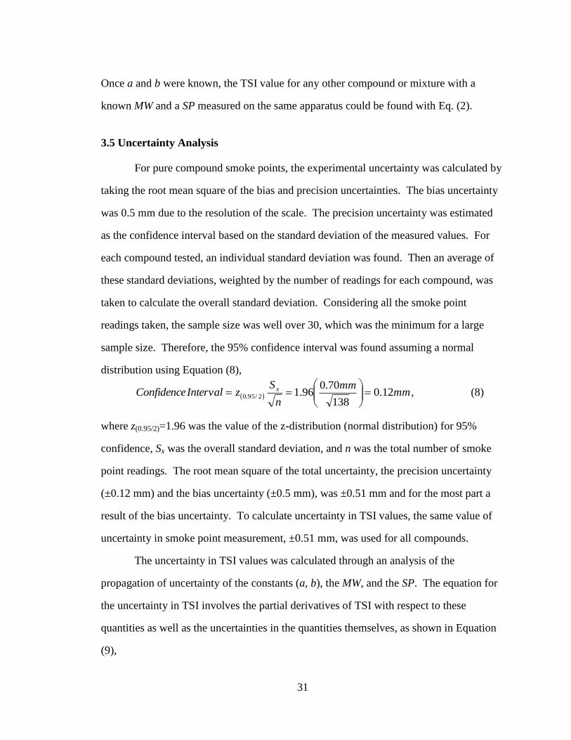
3.4 Procedure for TSI Calculation

Following the method described by Calcote and Manos [13], the set of TSI values

was based on the highest and lowest values of MW/SP from the measurements. A TSI

value of 100 was assigned to 1-methylnaphthalene, which had the highest MW/SP. The

lowest MW/SP from the data was for methylcyclohexane. The TSI value for

methylcyclohexane was chosen to be 5 because the suggested value reported in Ref. 13

for TSIMCH was 4.9±1.1. The apparatus specific constants could be found by solving for

a and b in the TSI equations for 1-methylnaphthalene and methylcyclohexane, Eq. (7),

bSP

MWa

bSP

MWa

MCH

MN

5

1001

. (7)

31

Once a and b were known, the TSI value for any other compound or mixture with a

known MW and a SP measured on the same apparatus could be found with Eq. (2).

3.5 Uncertainty Analysis

For pure compound smoke points, the experimental uncertainty was calculated by

taking the root mean square of the bias and precision uncertainties. The bias uncertainty

was 0.5 mm due to the resolution of the scale. The precision uncertainty was estimated

as the confidence interval based on the standard deviation of the measured values. For

each compound tested, an individual standard deviation was found. Then an average of

these standard deviations, weighted by the number of readings for each compound, was

taken to calculate the overall standard deviation. Considering all the smoke point

readings taken, the sample size was well over 30, which was the minimum for a large

sample size. Therefore, the 95% confidence interval was found assuming a normal

distribution using Equation (8),

mmmm

n

SzIntervalConfidence x 12.0

138

70.096.12/95.0

, (8)

where z(0.95/2)=1.96 was the value of the z-distribution (normal distribution) for 95%

confidence, Sx was the overall standard deviation, and n was the total number of smoke

point readings. The root mean square of the total uncertainty, the precision uncertainty

(±0.12 mm) and the bias uncertainty (±0.5 mm), was ±0.51 mm and for the most part a

result of the bias uncertainty. To calculate uncertainty in TSI values, the same value of

uncertainty in smoke point measurement, ±0.51 mm, was used for all compounds.

The uncertainty in TSI values was calculated through an analysis of the

propagation of uncertainty of the constants (a, b), the MW, and the SP. The equation for

the uncertainty in TSI involves the partial derivatives of TSI with respect to these

quantities as well as the uncertainties in the quantities themselves, as shown in Equation

(9),

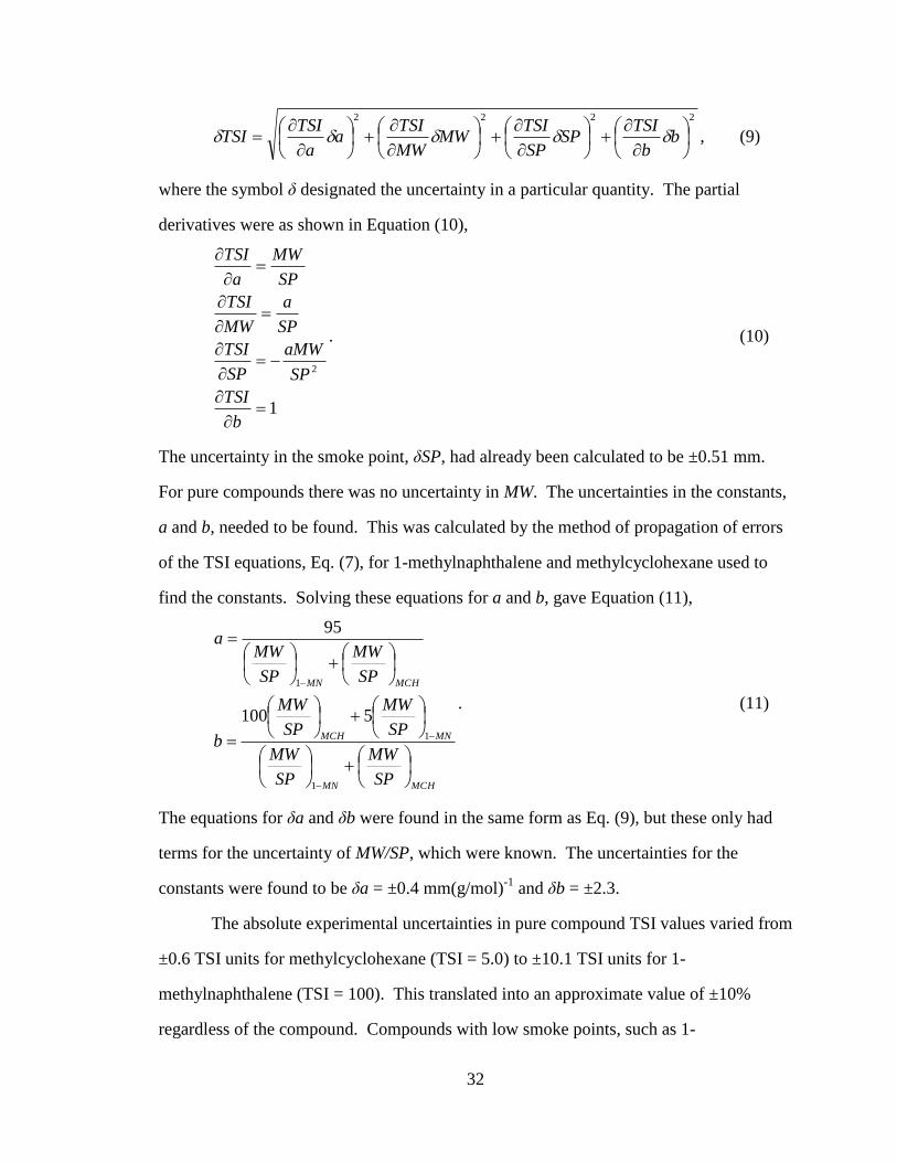
32

2222

b

b

TSISP

SP

TSIMW

MW

TSIa

a

TSITSI , (9)

where the symbol δ designated the uncertainty in a particular quantity. The partial

derivatives were as shown in Equation (10),

1

2

b

TSI

SP

aMW

SP

TSI

SP

a

MW

TSI

SP

MW

a

TSI

. (10)

The uncertainty in the smoke point, δSP, had already been calculated to be ±0.51 mm.

For pure compounds there was no uncertainty in MW. The uncertainties in the constants,

a and b, needed to be found. This was calculated by the method of propagation of errors

of the TSI equations, Eq. (7), for 1-methylnaphthalene and methylcyclohexane used to

find the constants. Solving these equations for a and b, gave Equation (11),

MCHMN

MNMCH

MCHMN

SP

MW

SP

MW

SP

MW

SP

MW

b

SP

MW

SP

MWa

1

1

1

5100

95

. (11)

The equations for δa and δb were found in the same form as Eq. (9), but these only had

terms for the uncertainty of MW/SP, which were known. The uncertainties for the

constants were found to be δa = ±0.4 mm(g/mol)-1

and δb = ±2.3.

The absolute experimental uncertainties in pure compound TSI values varied from

±0.6 TSI units for methylcyclohexane (TSI = 5.0) to ±10.1 TSI units for 1-

methylnaphthalene (TSI = 100). This translated into an approximate value of ±10%

regardless of the compound. Compounds with low smoke points, such as 1-

33

methylnaphthalene, tended to have larger absolute experimental errors, but these same

compounds tended to have larger TSI values. Conversely, compounds with high smoke

points, such as methylcyclohexane, tended to have smaller absolute experimental errors

and smaller TSI values.

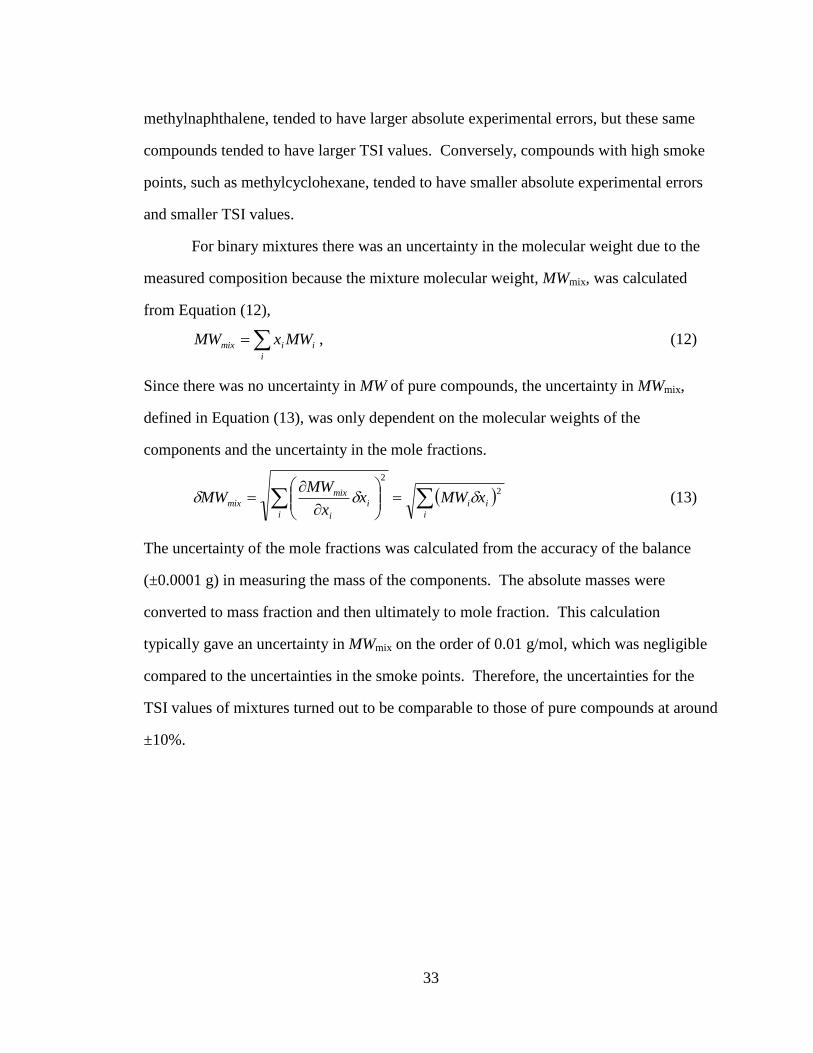
For binary mixtures there was an uncertainty in the molecular weight due to the

measured composition because the mixture molecular weight, MWmix, was calculated

from Equation (12),

i

iimix MWxMW , (12)

Since there was no uncertainty in MW of pure compounds, the uncertainty in MWmix,

defined in Equation (13), was only dependent on the molecular weights of the

components and the uncertainty in the mole fractions.

i

ii

i

i

i

mix

mix xMWxx

MWMW

2

2

(13)

The uncertainty of the mole fractions was calculated from the accuracy of the balance

(±0.0001 g) in measuring the mass of the components. The absolute masses were

converted to mass fraction and then ultimately to mole fraction. This calculation

typically gave an uncertainty in MWmix on the order of 0.01 g/mol, which was negligible

compared to the uncertainties in the smoke points. Therefore, the uncertainties for the

TSI values of mixtures turned out to be comparable to those of pure compounds at around

±10%.

34

CHAPTER 4 RESULTS AND DISCUSSION

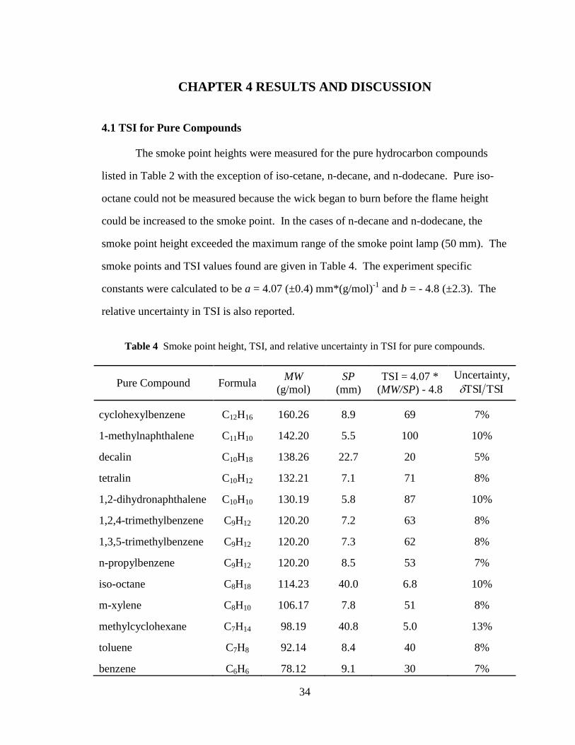
4.1 TSI for Pure Compounds

The smoke point heights were measured for the pure hydrocarbon compounds

listed in Table 2 with the exception of iso-cetane, n-decane, and n-dodecane. Pure iso-

octane could not be measured because the wick began to burn before the flame height

could be increased to the smoke point. In the cases of n-decane and n-dodecane, the

smoke point height exceeded the maximum range of the smoke point lamp (50 mm). The

smoke points and TSI values found are given in Table 4. The experiment specific

constants were calculated to be a = 4.07 (±0.4) mm*(g/mol)-1

and b = - 4.8 (±2.3). The

relative uncertainty in TSI is also reported.

Table 4 Smoke point height, TSI, and relative uncertainty in TSI for pure compounds.

Pure Compound Formula MW

(g/mol)

SP

(mm)

TSI = 4.07 *

(MW/SP) - 4.8

Uncertainty,

TSITSI

cyclohexylbenzene C12H16 160.26 8.9 69 7%

1-methylnaphthalene C11H10 142.20 5.5 100 10%

decalin C10H18 138.26 22.7 20 5%

tetralin C10H12 132.21 7.1 71 8%

1,2-dihydronaphthalene C10H10 130.19 5.8 87 10%

1,2,4-trimethylbenzene C9H12 120.20 7.2 63 8%

1,3,5-trimethylbenzene C9H12 120.20 7.3 62 8%

n-propylbenzene C9H12 120.20 8.5 53 7%

iso-octane C8H18 114.23 40.0 6.8 10%

m-xylene C8H10 106.17 7.8 51 8%

methylcyclohexane C7H14 98.19 40.8 5.0 13%

toluene C7H8 92.14 8.4 40 8%

benzene C6H6 78.12 9.1 30 7%

35

To supplement the set of TSI values for potential surrogate components, previous

TSI and YSI data sets were also considered. However, TSI values from the present study

were not directly comparable because the previously reported TSI and YSI values were

scaled differently. The first TSI scale, defined by Calcote and Manos [13], was based on

two compounds tested by Hunt [12], and subsequent data sets were scaled from the initial

TSI values corresponding to the Hunt data. Following the work by Calcote and Manos

[13], researchers scaled new TSI data based on the average of previously reported values.

To ensure consistent comparison of previous TSI results to those of this study, the scaling

procedure was redone based on the TSI data set shown in Table 4. To compare separate

data sets, it was required that at least two compounds be common to both studies. The

studies which fit this criterion are shown in Table 5. These sources measured different

parameters, including flame height at the smoke point, fuel mass flowrate at the smoke

point, and maximum soot volume fraction in the doped methane flame studied by

McEnally and Pfefferle [16, 17]. Table 5 also lists the units in which the data were

measured. The measured quantities were rearranged into parameters proportional to

sooting tendency (TSI or YSI), which are listed in the “TSI or YSI Parameter" column in

Table 5. The TSI values were determined using the method, described by Olson et al.

[14], of performing a linear regression between the TSI values in Table 4 and the

corresponding TSI or YSI parameters from each prior study. The resulting regression

equation defined the apparatus specific constants, a and b, and the R2 correlation

coefficient for each data set.

36

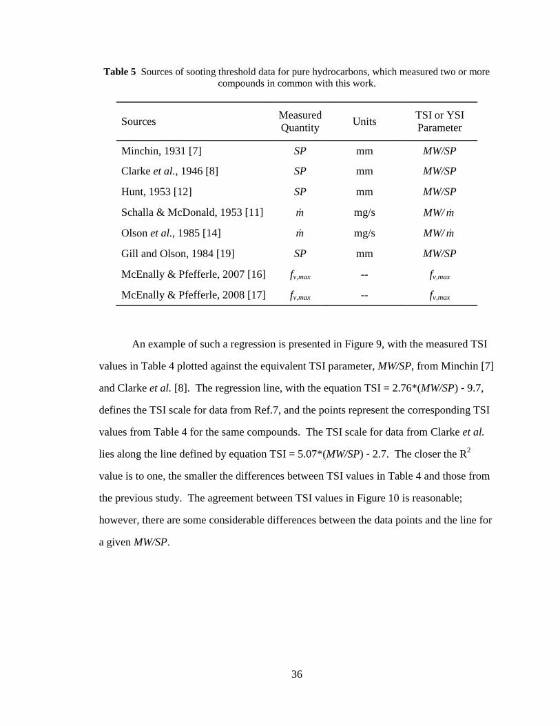
Table 5 Sources of sooting threshold data for pure hydrocarbons, which measured two or more

compounds in common with this work.

Sources Measured

Quantity Units

TSI or YSI

Parameter

Minchin, 1931 [7] SP mm MW/SP

Clarke et al., 1946 [8] SP mm MW/SP

Hunt, 1953 [12] SP mm MW/SP

Schalla & McDonald, 1953 [11] m mg/s MW/ m

Olson et al., 1985 [14] m mg/s MW/ m

Gill and Olson, 1984 [19] SP mm MW/SP

McEnally & Pfefferle, 2007 [16] fv,max -- fv,max

McEnally & Pfefferle, 2008 [17] fv,max -- fv,max

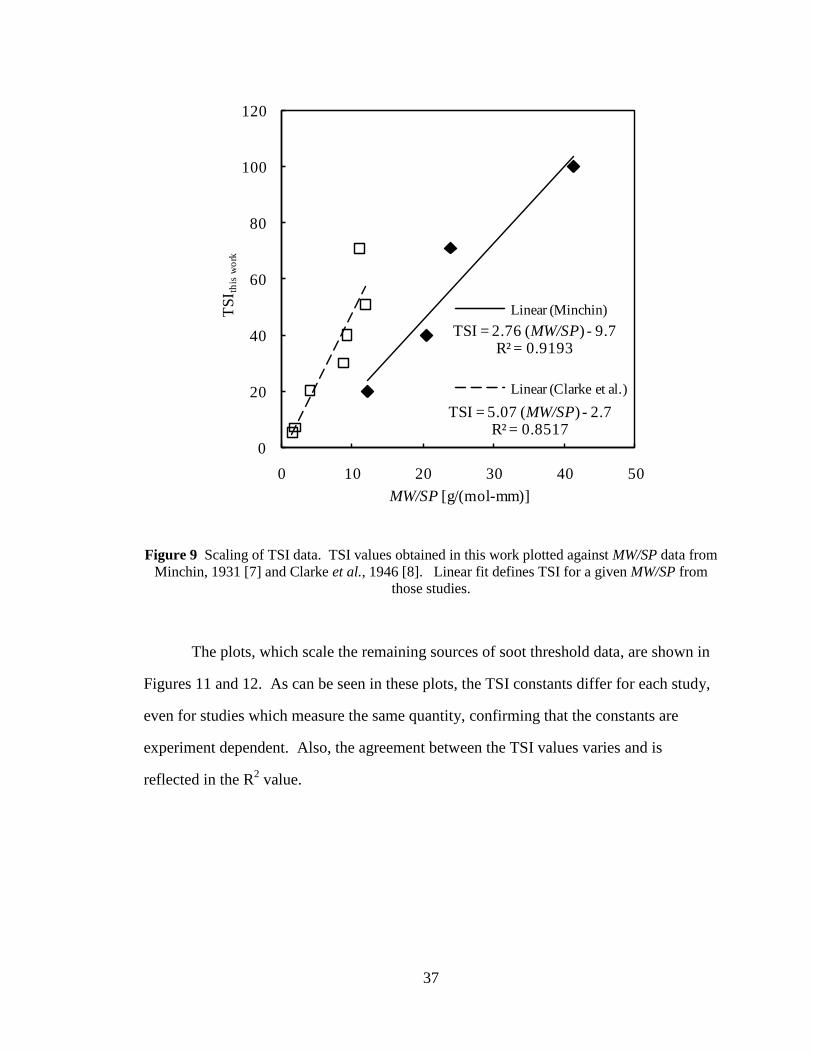
An example of such a regression is presented in Figure 9, with the measured TSI

values in Table 4 plotted against the equivalent TSI parameter, MW/SP, from Minchin [7]

and Clarke et al. [8]. The regression line, with the equation TSI = 2.76*(MW/SP) - 9.7,

defines the TSI scale for data from Ref.7, and the points represent the corresponding TSI

values from Table 4 for the same compounds. The TSI scale for data from Clarke et al.

lies along the line defined by equation TSI = 5.07*(MW/SP) - 2.7. The closer the R2

value is to one, the smaller the differences between TSI values in Table 4 and those from

the previous study. The agreement between TSI values in Figure 10 is reasonable;

however, there are some considerable differences between the data points and the line for

a given MW/SP.

37

TSI = 2.76 (MW/SP) - 9.7R² = 0.9193

TSI = 5.07 (MW/SP) - 2.7R² = 0.8517

0

20

40

60

80

100

120

0 10 20 30 40 50

TS

I th

is w

ork

MW/SP [g/(mol-mm)]

Linear (Minchin)

Linear (Clarke et al.)

Figure 9 Scaling of TSI data. TSI values obtained in this work plotted against MW/SP data from

Minchin, 1931 [7] and Clarke et al., 1946 [8]. Linear fit defines TSI for a given MW/SP from

those studies.

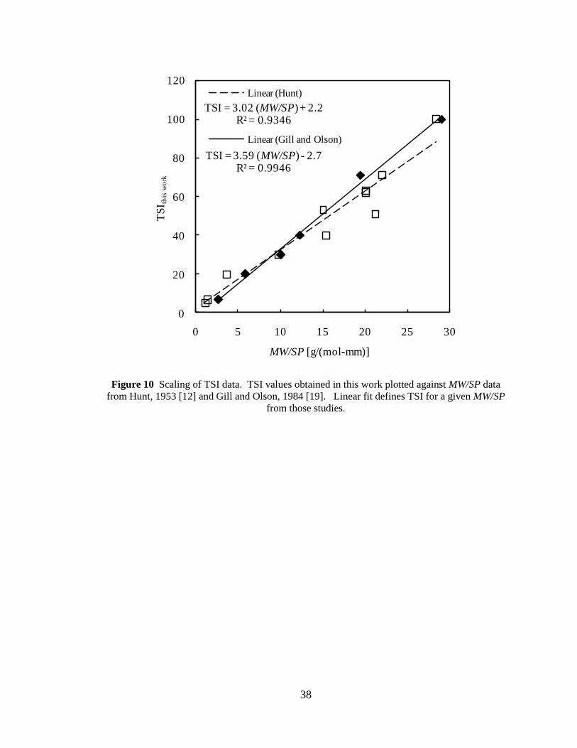
The plots, which scale the remaining sources of soot threshold data, are shown in

Figures 11 and 12. As can be seen in these plots, the TSI constants differ for each study,

even for studies which measure the same quantity, confirming that the constants are

experiment dependent. Also, the agreement between the TSI values varies and is

reflected in the R2 value.

38

TSI = 3.02 (MW/SP) + 2.2R² = 0.9346

TSI = 3.59 (MW/SP) - 2.7R² = 0.9946

0

20

40

60

80

100

120

0 5 10 15 20 25 30

TS

I th

is w

ork

MW/SP [g/(mol-mm)]

Linear (Hunt)

Linear (Gill and Olson)

Figure 10 Scaling of TSI data. TSI values obtained in this work plotted against MW/SP data

from Hunt, 1953 [12] and Gill and Olson, 1984 [19]. Linear fit defines TSI for a given MW/SP

from those studies.

39

TSI = 0.0468 (MW/ )+ 20.1R² = 0.9935

TSI = 0.111 (MW/ ) + 1.5R² = 0.9602

0

20

40

60

80

100

120

0 200 400 600 800 1000

TS

I th

is w

ork

MW/ [(g/mol)*(mg/s)-1]

Linear (Schalla & McDonald)

Linear (Olson et al.)

m

m

m

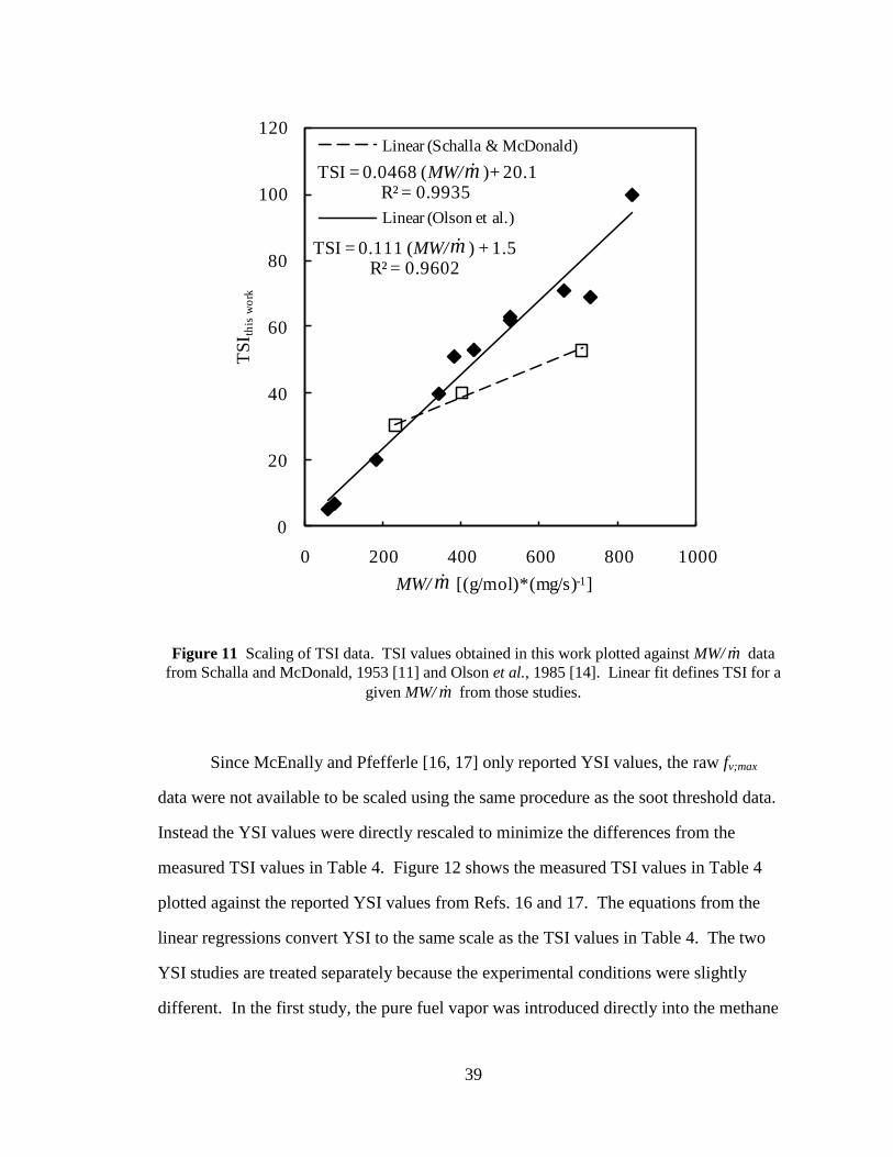
Figure 11 Scaling of TSI data. TSI values obtained in this work plotted against MW/ m data

from Schalla and McDonald, 1953 [11] and Olson et al., 1985 [14]. Linear fit defines TSI for a

given MW/ m from those studies.

Since McEnally and Pfefferle [16, 17] only reported YSI values, the raw fv;max

data were not available to be scaled using the same procedure as the soot threshold data.

Instead the YSI values were directly rescaled to minimize the differences from the

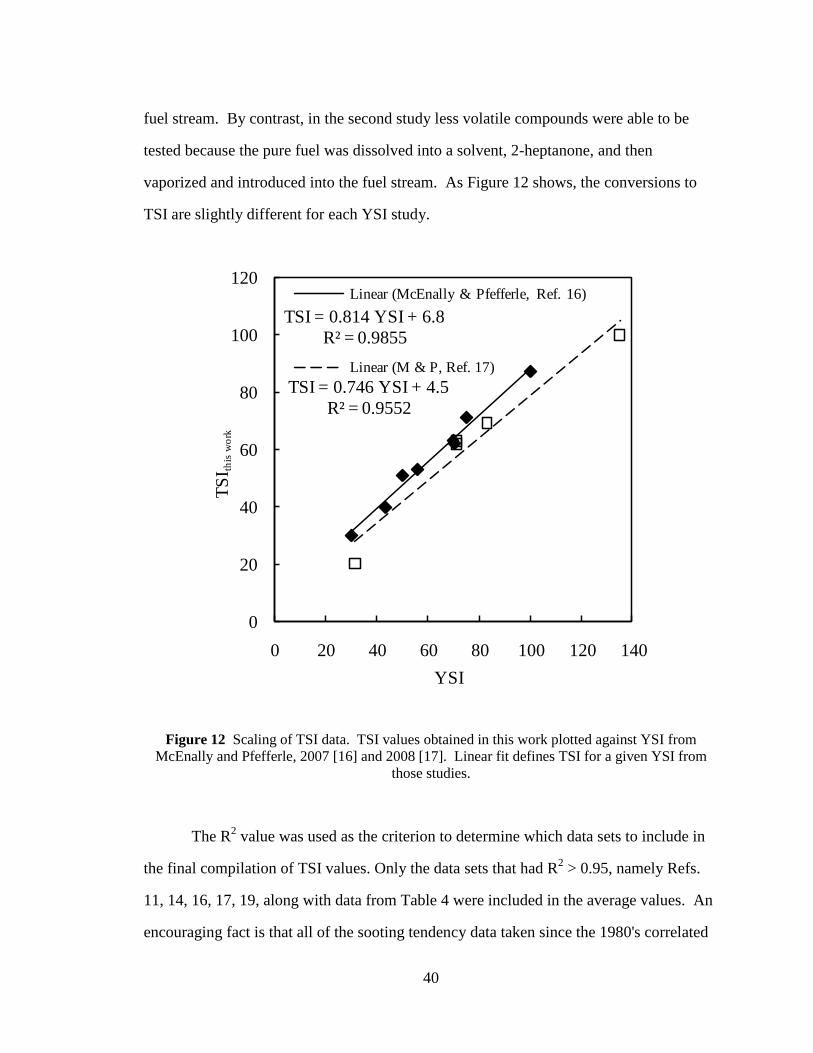
measured TSI values in Table 4. Figure 12 shows the measured TSI values in Table 4

plotted against the reported YSI values from Refs. 16 and 17. The equations from the

linear regressions convert YSI to the same scale as the TSI values in Table 4. The two

YSI studies are treated separately because the experimental conditions were slightly

different. In the first study, the pure fuel vapor was introduced directly into the methane

40

fuel stream. By contrast, in the second study less volatile compounds were able to be

tested because the pure fuel was dissolved into a solvent, 2-heptanone, and then

vaporized and introduced into the fuel stream. As Figure 12 shows, the conversions to

TSI are slightly different for each YSI study.

TSI = 0.814 YSI + 6.8

R² = 0.9855

TSI = 0.746 YSI + 4.5

R² = 0.9552

0

20

40

60

80

100

120

0 20 40 60 80 100 120 140

TS

I th

is w

ork

YSI

Linear (McEnally & Pfefferle, Ref. 16)

Linear (M & P, Ref. 17)

Figure 12 Scaling of TSI data. TSI values obtained in this work plotted against YSI from

McEnally and Pfefferle, 2007 [16] and 2008 [17]. Linear fit defines TSI for a given YSI from

those studies.

The R2 value was used as the criterion to determine which data sets to include in

the final compilation of TSI values. Only the data sets that had R2 > 0.95, namely Refs.

11, 14, 16, 17, 19, along with data from Table 4 were included in the average values. An

encouraging fact is that all of the sooting tendency data taken since the 1980's correlated

41

well with the data measured here. With the exception of the work of Schalla &

McDonald, the older studies did not correlate as well.

The rescaled TSI values, the experimental constants, and the average TSI values,

are shown in Table 6. The TSI values for the compounds for which smoke points could

not be measured with the ASTM standard apparatus were obtained other ways. The TSI

values of n-decane and n-dodecane were found from the study by Olson et al. [14], in

which they measured the smoke point mass flowrate in an apparatus that could handle

higher smoke points than the ASTM apparatus. As for iso-cetane, no smoke point

measurements were found in the literature. However, Yan et al. [15] did provide an

estimated TSI value of iso-cetane based on a polynomial regression model that correlated

known TSI values with structural groups present in the fuel molecule. From the

correlation, they estimated iso-cetane had a TSI of 14.6. In the present study, a method

was developed using binary mixtures to check the estimated TSI from Yan et al., as

discussed in section 4.2.

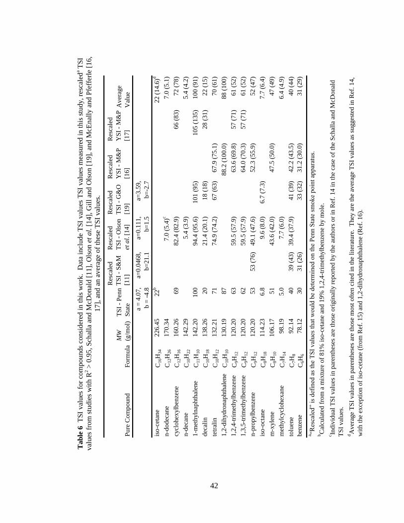
42

Tab

le 6

T

SI

val

ues

for

com

po

unds

consi

der

ed i

n t

his

work

. D

ata

incl

ude

TS

I val

ues

TS

I val

ues

mea

sure

d i

n t

his

stu

dy

, re

scal

eda T

SI

val

ues

fro

m s

tud

ies

wit

h R

2 >

0.9

5,

Sch

alla

and

McD

onal

d [

11],

Ols

on e

t al.

[14],

Gil

l an

d O

lso

n [

19],

an

d M

cEn

ally

an

d P

feff

erle

[1

6,

17],

and a

n a

ver

age

of

thes

e T

SI

val

ues

.

Pu

re C

om

po

un

dF

orm

ula

MW

(g/m

ol)

TS

I -

Pen

n

Sta

te

Res

cale

d

TS

I -

S&

M

[11

]

Res

cale

d

TS

I -

Ols

on

et a

l.[1

4]

Res

cale

d

TS

I -

G&

O

[19

]

Res

cale

d

YS

I -

M&

P

[16

]

Res

cale

d

YS

I -

M&

P

[17

]

Av

erag

e

Val

ue

a =

4.0

7,

b =

-4

.8

a=0

.04

68

,

b=

21

.1

a=0

.11

1,

b=

1.5

a=3

.59

,

b=

-2.7

iso

-cet

ane

C1

6H

34

22

6.4

52

2b

22

(14

.6)d

n-d

od

ecan

eC

12H

26

17

0.3

47

.0 (

5.4

)c7

.0 (

5.1

)

cycl

oh

exylb

enze

ne

C1

2H

16

16

0.2

66

98

2.4

(8

2.9

)6

6 (

83

)7

2 (

78

)

n-d

ecan

eC

10H

22

14

2.2

95

.4 (

3.9

)5

.4 (

4.2

)

1-m

eth

yln

aph

thal

ene

C1

1H

10

14

2.2

01

00

94

.4 (

95

.6)

10

1 (

95

)1

05

(1

35

)1

00

(9

1)

dec

alin

C1

0H

18

13

8.2

62

02

1.4

(2

0.1

)1

8 (

18

)2

8 (

31

)2

2 (

15

)

tetr

alin

C1

0H

12

13

2.2

17

17

4.9

(7

4.2

)6

7 (

63

)6

7.9

(7

5.1

)7

0 (

61

)

1,2

-dih

yd

ron

aph

thal

ene

C1

0H

10

13

0.1

98

78

8.2

(1

00

.0)

88

(10

0)

1,2

,4-t

rim

eth

ylb

enze

ne

C9H

12

12

0.2

06

35

9.5

(5

7.9

)6

3.6

(6

9.8

)5

7 (

71

)6

1 (

52

)

1,3

,5-t

rim

eth

ylb

enze

ne

C9H

12

12

0.2

06

25

9.5

(5

7.9

)6

4.0

(7

0.3

)5

7 (

71

)6

1 (

52

)

n-p

rop

ylb

enze

ne

C9H

12

12

0.2

05

35

3 (

76

)4

9.1

(4

7.6

)5

2.3

(5

5.9

)5

2 (

47

)

iso

-oct

ane

C8H

18

11

4.2

36

.89

.6 (

8.0

)6

.7 (

7.3

)7

.7 (

6.4

)

m-x

yle

ne

C8H

10

10

6.1

75

14

3.6

(4

2.0

)4

7.5

(5

0.0

)4

7 (

49

)

met

hylc

ycl

oh

exan

eC

7H

14

98

.19

5.0

7.7

(6.0

)6

.4 (

4.9

)

tolu

ene

C7H

89

2.1

44

03

9 (

43

)3

9.4

(3

7.9

)4

1 (

39

)4

2.2

(4

3.5

)4

0 (

44

)

ben

zen

eC

6H

67

8.1

23

03

1 (

26

)3

3 (

32

)3

1.2

(3

0.0

)3

1 (

29

)

a “Res

cale

d”

is d

efin

ed a

s th

e T

SI

val

ues

th

at w

ou

ld b

e d

eter

min

ed o

n t

he

Pen

n S

tate

sm

ok

e p

oin

t ap

par

atu

s.bC

alcu

late

d f

rom

a m

ixtu

re o

f 8

1%

iso

-cet

ane

and

19

% 1

,2,4

-tri

met

hylb

enze

ne

by m

ole

.

c Ind

ivid

ual

TS

I v

alu

es i

n p

aren

thes

es a

re t

ho

se o

rigin

ally

rep

ort

ed b

y t

he

auth

ors

or

in R

ef.

14

in

th

e ca

se o

f th

e S

chal

la a

nd

McD

on

ald

TS

I v

alu

es.

dA

ver

age

TS

I v

alu

es i

n p

aren

thes

es a

re t

ho

se m

ost

oft

en c

ited

in

th

e li

tera

ture

. T

hey

are

th

e av

erag

e T

SI

val

ues

as

sugges

ted

in

Ref

. 1

4,

wit

h t

he

exce

pti

on

of

iso

-cet

ane

(fro

m R

ef.

15

) an

d 1

,2-d

ihyd

ron

aph

thal

ene

(Ref

. 1

6).

43

In Table 6, the previous TSI values as they were reported in Refs. 14, 16, 17, and

19 are shown in parentheses for comparison. Although the data sets from Refs. 14 and 19

have not changed much from their original values, the other three data sets did change

significantly with the rescaling. Because TSI and YSI are relative parameters, the

absolute quantities depend on the compounds and original values used to define the scale.

For Schalla and McDonald [11], the TSI was originally scaled using more

compounds than the ones listed, and TSI is sensitive to the quality of each data point

included. Because of the inherent subjectivity of the smoke point measurement, this

could be an issue. The quality of any of these data is unknown, and the best way to

assess whether two studies obtained similar results is to find the correlation between the

compounds in common, as was done here. The rescaling of the three compounds in

common with this work, acted to shift the TSI values of the aromatics tested by Schalla

and McDonald almost exactly to the TSI values measured here, and therefore meeting the

criterion that had been set.

The differences observed for the YSI data sets can be explained by the original

values used to define the scale. For the first YSI data set, the original scale was defined

assuming a TSI of 100 for 1,2-dihydronaphthalene. By contrast, here the TSI of 1-

methylnaphthalene was set to 100. In the second YSI data set, 1-methylnaphthalene

turned out to have a higher TSI than 1,2-dihydronaphthalene. Therefore, in the rescaling

both YSI data sets are lower than the original reported values.

In parentheses next to the average TSI values in Table 6 are the TSI values

suggested by Olson et al. [14], except for iso-cetane and 1,2-dihydronaphthalene, which

were not included in Ref. 14. For iso-cetane, it is the TSI estimated in Ref. 15, and for

1,2-dihydronaphthalene, it is the YSI measured in Ref. 16. The set of TSI values in

parentheses is the set of TSI values most often cited in the literature. To show that the

rescaling procedure has reduced deviations in TSI values, the total root mean square

deviation from the average TSI values was calculated. For the rescaled TSI values, the

44

root mean square deviation was 3.0 TSI units, as compared to 7.5 TSI units for the values

in parentheses.

Some of the major changes in average TSI values were for the three C9H12

aromatic compounds, 1-methylnaphthalene, and 1,2-dihydronaphthalene. The TSI values

for propylbenzene and both trimethylbenzenes increased by more than 10%. The

deviation between studies in Table 6 was ±4 TSI units for four studies, rather than ±6 TSI

units for two studies cited in Olson et al. [14].

The average TSI for 1-methylnaphthalene, 100, as opposed to 91 from Ref. 14,

reflects the original TSI assigned to it. In Calcote and Manos, a linear adjustment that

reduced the TSI of 1-methylnaphthalene, was made to keep the scale within 0 and 100.

Although not included in the previous TSI average suggested by Olson et al., the YSI of

1-methylnaphthalene was 135 when McEnally and Pfefferle chose to assign 1,2-

dihydronaphthalene a YSI of 100. With the YSI studies rescaled using more than two

compounds, the YSI of 1-methylnaphthalene reduced to within ±10% of 100. Since the

previously reported average TSI (91) and YSI (135) for 1-methylnaphthalene were so

different, it could have been argued that the two sooting tendency parameters were not

comparable. However, the rescaling of these studies shows that TSI and YSI are

complementary measures of sooting tendency, when considering the compounds in

Table 6.

Another consequence of the rescaling of the YSI data was that the TSI of 1,2-

dihydronaphthalene reduced from 100 to 88. However, according to Hunt’s results, the

TSI of naphthalene was higher than 1-methylnaphthalene, and McEnally and Pfefferle

showed that 1,2-dihydronaphthalene and naphthalene were equivalent in YSI. Therefore,

either the smoke points found by Hunt are not correct, or the TSI values of 1,2-

dihydronaphthalene and naphthalene are not equivalent. Further studies on the TSI of

naphthalene, which is a solid at room temperature, are needed to confirm this.

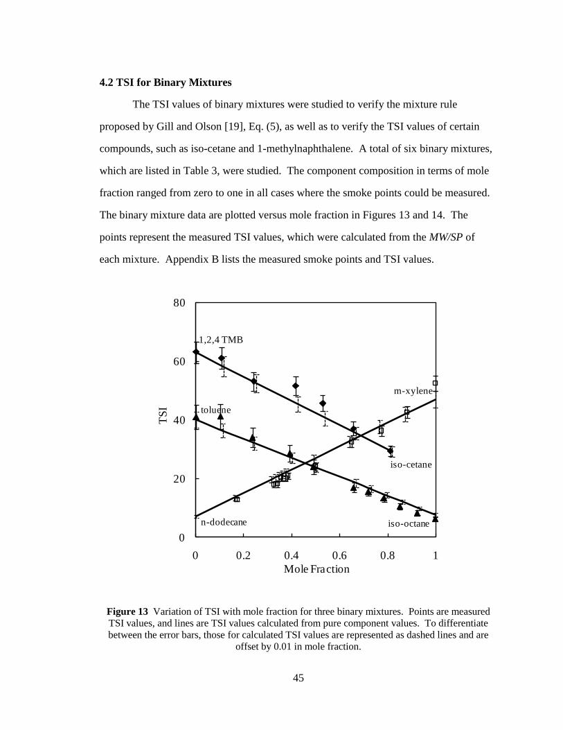
45

4.2 TSI for Binary Mixtures

The TSI values of binary mixtures were studied to verify the mixture rule

proposed by Gill and Olson [19], Eq. (5), as well as to verify the TSI values of certain

compounds, such as iso-cetane and 1-methylnaphthalene. A total of six binary mixtures,

which are listed in Table 3, were studied. The component composition in terms of mole

fraction ranged from zero to one in all cases where the smoke points could be measured.

The binary mixture data are plotted versus mole fraction in Figures 13 and 14. The

points represent the measured TSI values, which were calculated from the MW/SP of

each mixture. Appendix B lists the measured smoke points and TSI values.

0

20

40

60

80

0 0.2 0.4 0.6 0.8 1

TS

I

Mole Fraction

m-xylene

toluene

iso-cetane

1,2,4 TMB

n-dodecane iso-octane

Figure 13 Variation of TSI with mole fraction for three binary mixtures. Points are measured

TSI values, and lines are TSI values calculated from pure component values. To differentiate

between the error bars, those for calculated TSI values are represented as dashed lines and are

offset by 0.01 in mole fraction.

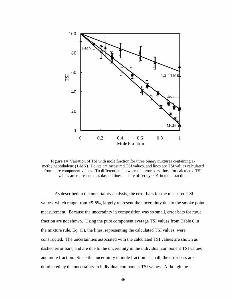
46

0

20

40

60

80

100

0 0.2 0.4 0.6 0.8 1

TS

I

Mole Fraction

1,2,4 TMB

1-MN

MCH

decalin

Figure 14 Variation of TSI with mole fraction for three binary mixtures containing 1-

methylnaphthalene (1-MN). Points are measured TSI values, and lines are TSI values calculated

from pure component values. To differentiate between the error bars, those for calculated TSI

values are represented as dashed lines and are offset by 0.01 in mole fraction.

As described in the uncertainty analysis, the error bars for the measured TSI

values, which range from ±5-8%, largely represent the uncertainty due to the smoke point

measurement. Because the uncertainty in composition was so small, error bars for mole

fraction are not shown. Using the pure component average TSI values from Table 6 in

the mixture rule, Eq. (5), the lines, representing the calculated TSI values, were

constructed. The uncertainties associated with the calculated TSI values are shown as

dashed error bars, and are due to the uncertainty in the individual component TSI values

and mole fraction. Since the uncertainty in mole fraction is small, the error bars are

dominated by the uncertainty in individual component TSI values. Although the

47

individual component TSI values used were the average values listed in Table 6, the

uncertainty was taken to be the same as the uncertainty estimated for the data found in

this study. The total uncertainty in the predicted mixture TSI values (±6-9%) was

generally about the same as the measured TSI mixture uncertainty. For all the mixtures

tested, the error bars of the measured TSI points lie within the error bars of the calculated

TSI line. It can then be concluded that the linear mixture rule, Eq. (5), applied to these

mixtures in addition to the mixtures already reported in Ref. 19.

One binary mixture, 1-methylnaphthalene/decalin was also studied in Gill and

Olson [19]. Examination of the three mixture data points taken in Ref. 19 to the TSI

values found for comparable mixtures shows that they are very similar to those found

here. The experimental constants that were used, a = 3.32 mm*(g/mol)-1

, b = -1.47, are

similar to the rescaled constants found in this study for Ref. 19, a = 3.59 mm*(g/mol)-1

, b

= -2.7. Therefore the TSI values using the new scale are similar to the TSI values

reported using the original Gill and Olson scale.

To derive a TSI value for pure iso-cetane, a binary mixture containing as much

iso-cetane as possible without losing the ability to measure the smoke point was tested.

The mixture contained 81% iso-cetane and 19% 1,2,4-trimethylbenzene, molar mixture.

Based on the linear mixture rule, Eq. (5), the TSI of the mixture was equal to the linear

sum of the component's individual TSI values weighted by their mole fractions, called

TSIcalc, defined for this mixture in Eq. (13). The TSI of the mixture was also found from

the MW and SP of the mixture, called TSImeas, defined in Eq. (14). As a component of the

mixture, iso-cetane's TSI was found by equating the TSImeas to the TSIcalc, and solving for

TSIi-cet in Eq. (13).

ceticetiTMBTMBcalc xTSIxTSITSI 4,2,14,2,1 (13)

bSPMWaTSI mixmixmeas (14)

This calculation yielded a TSI for iso-cetane of 22. This is about seven TSI units (51%)

higher than the value estimated by Yan et al. [15]. When the measured TSI values were

48

compared with the calculated TSI values using 22 for iso-cetane, the error bars

overlapped as seen in Figure 13.

Three binary mixtures containing 1-methylnaphthalene were tested to obtain

additional data on its pure compound TSI value. Since 1-methylnaphthalene had the

highest MW/SP, it was one of the two compounds that were assigned a TSI value.

Therefore, the MW/SP for 1-methylnaphthalene partly defined the scale for the rest of the

compounds. Unlike the other end point of the scale, methylcyclohexane, 1-

methylnaphthalene had a very small smoke point height, around 5 mm. Because of the

low flowrate associated with a smoke point of this height, this short flame was very

stable, and the smoke point was easy to identify. However, the uncertainty was large

because the resolution of the scale was only 1 mm. By mixing 1-methylnaphthalene with

compounds that have a higher smoke point, the relative error in the smoke point

measurement could be reduced. Because the mixture points with the highest 1-

methylnaphthalene content still had very low smoke points, all the mixtures containing

any 1-methylnaphthalene were used to derive its TSI.

A TSI value was obtained for 1-methylnapthalene by taking linear fits to all the

measured points for the three binary mixtures, as shown in Figure 15. If the fit line is

extrapolated back to the point where the mixture is entirely 1-methylnaphthalene, a TSI

for 1-methylnaphthalene can be obtained. This is equivalent to inserting zero for the

mole fraction of the other component in the equations of the fit lines in Figure 15. For

the mixtures with 1,2,4-trimethylbenzene, decalin, and methylcyclohexane, the calculated

TSI values for 1-methylnaphthalene were 94, 100, and 102, respectively. These values

were well within the estimated uncertainty of ±10% of 100, the TSI found for the pure

compound. Therefore, the calculated TSI values were consistent with its assigned TSI of

100.

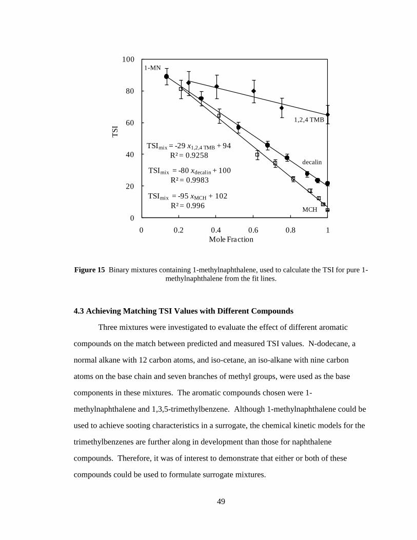
49

TSImix = -29 x1,2,4 TMB + 94

R² = 0.9258

TSImix = -95 xMCH + 102

R² = 0.996

TSImix = -80 xdecalin + 100

R² = 0.9983

0

20

40

60

80

100

0 0.2 0.4 0.6 0.8 1

TS

I

Mole Fraction

1,2,4 TMB

1-MN

MCH

decalin

Figure 15 Binary mixtures containing 1-methylnaphthalene, used to calculate the TSI for pure 1-

methylnaphthalene from the fit lines.

4.3 Achieving Matching TSI Values with Different Compounds

Three mixtures were investigated to evaluate the effect of different aromatic

compounds on the match between predicted and measured TSI values. N-dodecane, a

normal alkane with 12 carbon atoms, and iso-cetane, an iso-alkane with nine carbon

atoms on the base chain and seven branches of methyl groups, were used as the base

components in these mixtures. The aromatic compounds chosen were 1-

methylnaphthalene and 1,3,5-trimethylbenzene. Although 1-methylnaphthalene could be

used to achieve sooting characteristics in a surrogate, the chemical kinetic models for the

trimethylbenzenes are further along in development than those for naphthalene

compounds. Therefore, it was of interest to demonstrate that either or both of these

compounds could be used to formulate surrogate mixtures.

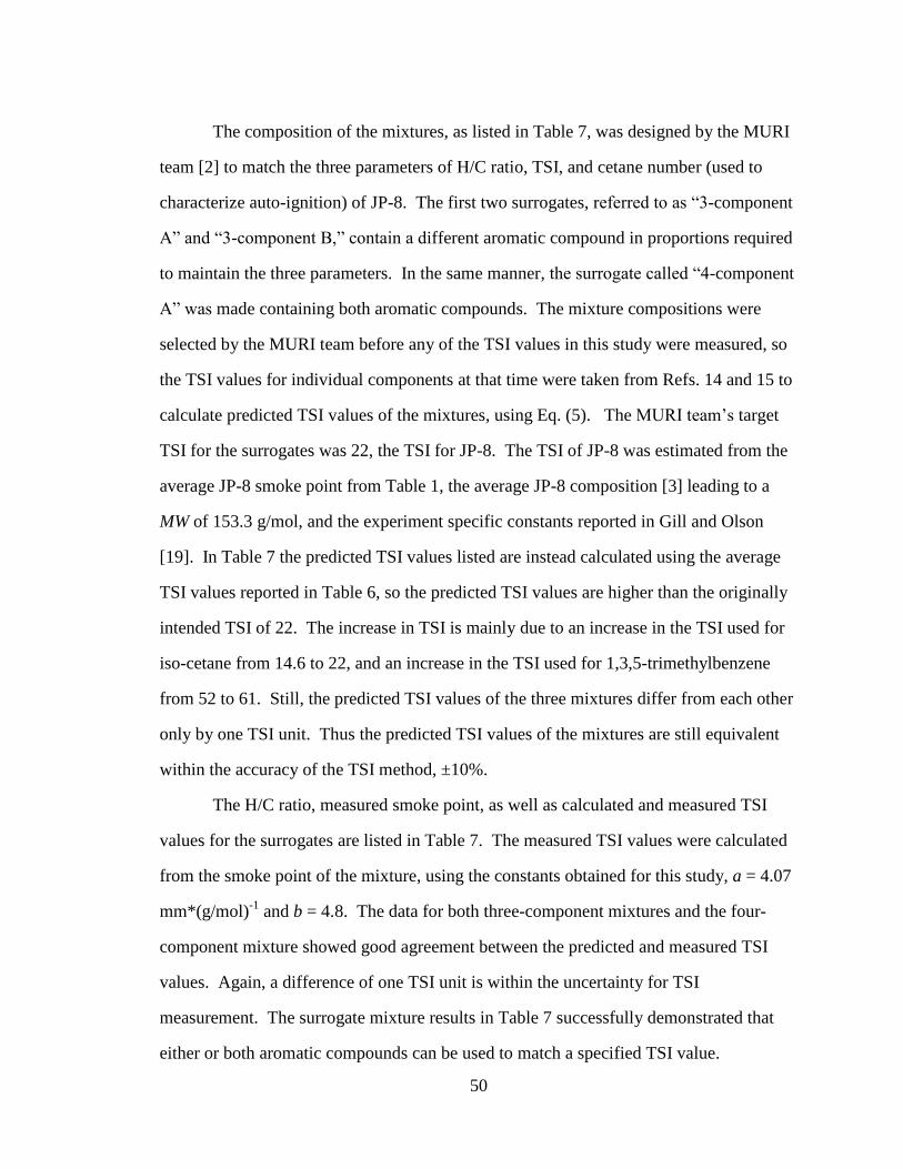
50

The composition of the mixtures, as listed in Table 7, was designed by the MURI

team [2] to match the three parameters of H/C ratio, TSI, and cetane number (used to

characterize auto-ignition) of JP-8. The first two surrogates, referred to as “3-component

A” and “3-component B,” contain a different aromatic compound in proportions required

to maintain the three parameters. In the same manner, the surrogate called “4-component

A” was made containing both aromatic compounds. The mixture compositions were

selected by the MURI team before any of the TSI values in this study were measured, so

the TSI values for individual components at that time were taken from Refs. 14 and 15 to

calculate predicted TSI values of the mixtures, using Eq. (5). The MURI team’s target

TSI for the surrogates was 22, the TSI for JP-8. The TSI of JP-8 was estimated from the

average JP-8 smoke point from Table 1, the average JP-8 composition [3] leading to a

MW of 153.3 g/mol, and the experiment specific constants reported in Gill and Olson

[19]. In Table 7 the predicted TSI values listed are instead calculated using the average

TSI values reported in Table 6, so the predicted TSI values are higher than the originally

intended TSI of 22. The increase in TSI is mainly due to an increase in the TSI used for

iso-cetane from 14.6 to 22, and an increase in the TSI used for 1,3,5-trimethylbenzene

from 52 to 61. Still, the predicted TSI values of the three mixtures differ from each other

only by one TSI unit. Thus the predicted TSI values of the mixtures are still equivalent

within the accuracy of the TSI method, ±10%.

The H/C ratio, measured smoke point, as well as calculated and measured TSI

values for the surrogates are listed in Table 7. The measured TSI values were calculated

from the smoke point of the mixture, using the constants obtained for this study, a = 4.07

mm*(g/mol)-1

and b = 4.8. The data for both three-component mixtures and the four-

component mixture showed good agreement between the predicted and measured TSI

values. Again, a difference of one TSI unit is within the uncertainty for TSI

measurement. The surrogate mixture results in Table 7 successfully demonstrated that

either or both aromatic compounds can be used to match a specified TSI value.

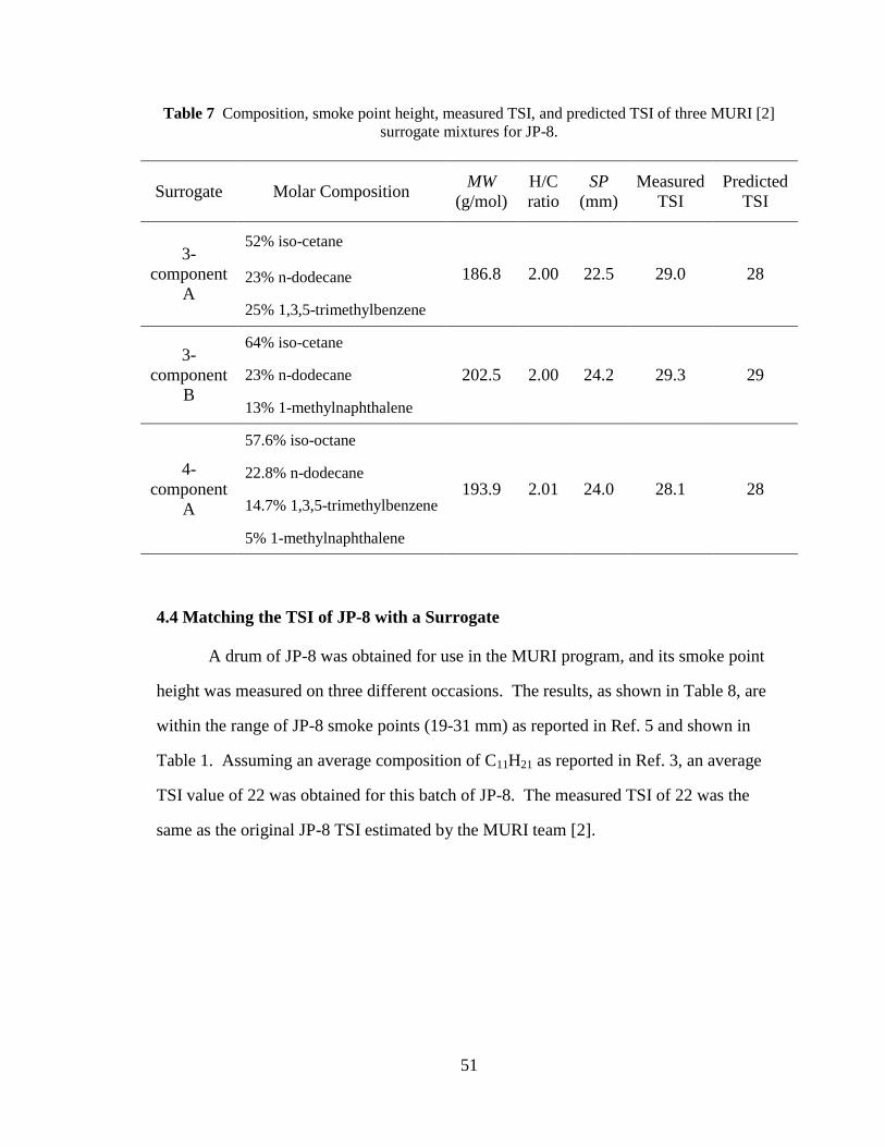
51

Table 7 Composition, smoke point height, measured TSI, and predicted TSI of three MURI [2]

surrogate mixtures for JP-8.

Surrogate Molar Composition MW

(g/mol)

H/C

ratio

SP

(mm)

Measured

TSI

Predicted

TSI

3-

component

A

52% iso-cetane

186.8 2.00 22.5 29.0 28 23% n-dodecane

25% 1,3,5-trimethylbenzene

3-

component

B

64% iso-cetane

202.5 2.00 24.2 29.3 29 23% n-dodecane

13% 1-methylnaphthalene

4-

component

A

57.6% iso-octane

193.9 2.01 24.0 28.1 28 22.8% n-dodecane

14.7% 1,3,5-trimethylbenzene

5% 1-methylnaphthalene

4.4 Matching the TSI of JP-8 with a Surrogate

A drum of JP-8 was obtained for use in the MURI program, and its smoke point

height was measured on three different occasions. The results, as shown in Table 8, are

within the range of JP-8 smoke points (19-31 mm) as reported in Ref. 5 and shown in

Table 1. Assuming an average composition of C11H21 as reported in Ref. 3, an average

TSI value of 22 was obtained for this batch of JP-8. The measured TSI of 22 was the

same as the original JP-8 TSI estimated by the MURI team [2].

52

Table 8 Smoke point height and TSI results for JP-8 samples taken from the same batch of fuel.

MW (g/mol)

estimated

SP

(mm)

Measured

TSI

JP-8 153.3 22.8 22.6

JP-8 153.3 22.2 23.3

JP-8 153.3 23.8 21.4

Average 153.3 23.0 22

A fourth surrogate mixture was devised with a target TSI of 22, and a target H/C

ratio between 1.844 and 2.067 [5]. This mixture, called “JP-8 surrogate (22),” is defined

in Table 9. This mixture was comprised of n-dodecane, iso-octane, and 1,3,5-

trimethylbenzene. Although these three components were chosen, it would have been

possible to design the surrogate with other components, e.g. n-dodecane, iso-cetane, and

1-methylnaphthalene. Iso-octane was used because it has a lower TSI value than iso-

cetane. In addition to iso-cetane, iso-octane was also being considered as a potential base

iso-alkane, and it was desired to show that measured and predicted TSI would still match

with an iso-octane surrogate. As shown in Table 9, the measured and predicted TSI

values differ by two TSI units. Although this difference is larger than the mixtures

presented in Table 7, it is within ±10%. These results indicated that a surrogate fuel

composed of only a few components can be formulated to match the sooting tendency of

JP-8.

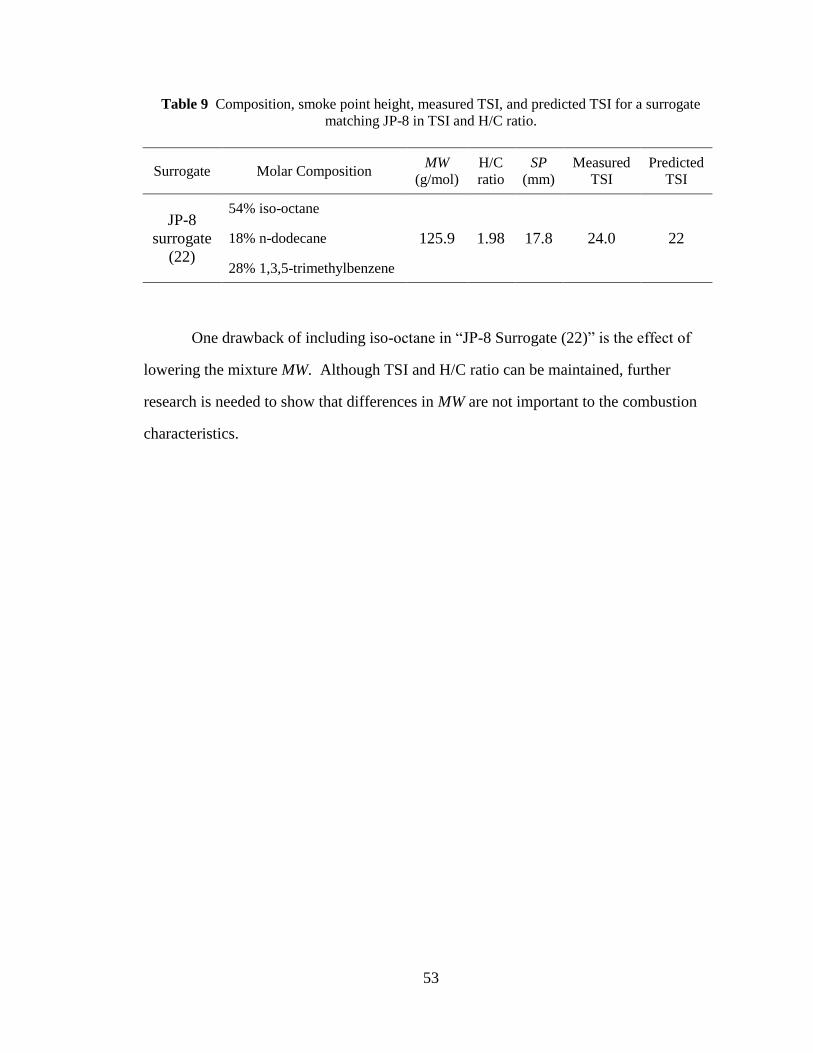
53

Table 9 Composition, smoke point height, measured TSI, and predicted TSI for a surrogate

matching JP-8 in TSI and H/C ratio.

Surrogate Molar Composition MW

(g/mol)

H/C

ratio

SP

(mm)

Measured

TSI

Predicted

TSI

JP-8

surrogate

(22)

54% iso-octane

125.9 1.98 17.8 24.0 22 18% n-dodecane

28% 1,3,5-trimethylbenzene

One drawback of including iso-octane in “JP-8 Surrogate (22)” is the effect of

lowering the mixture MW. Although TSI and H/C ratio can be maintained, further

research is needed to show that differences in MW are not important to the combustion

characteristics.

54

CHAPTER 5 CONCLUSIONS

Sooting tendency is an important parameter to consider in the design of jet fuel

surrogates. TSI was used to characterize sooting tendency for potential surrogate

components and their mixtures. Measurements of smoke point heights were taken

according to ASTM D1322 for sixteen pure hydrocarbons, including most of the potential

surrogate components being considered by the MURI team. From these data, TSI values

were derived, and the uncertainty was calculated to be approximately ±10%. Previous

literature data on soot threshold and soot yield of pure hydrocarbons were brought

together and compared on a common scale defined by the TSI values obtained in this

study. Previous data sets that had a satisfactory R2 correlation were retained to be

averaged into a consistent set of TSI and YSI values for pure hydrocarbon compounds.

In some cases, the scaling procedure had a significant effect on the TSI values previously

reported, to the point where the average TSI values changed by as much as 47%. The

scaling procedure resulted in better agreement between TSI values from different studies.

Therefore, when properly rescaled, a consistent set of TSI values can be assembled that

uses results from different studies. Although YSI values for sooting tendency are

obtained by a very different approach than TSI, both TSI and YSI data can be included in

the consistent set of sooting tendency values when rescaled.

The TSI values of several mixtures were determined to verify the rule used to

predict TSI values of mixtures, that the mixture TSI is the linear sum of the component

TSI values weighted by mole fraction. Within the estimated uncertainty, the

experimental TSI values of the binary mixtures as well as three and four component

mixtures matched the predicted TSI values. Therefore, using the consistent set of TSI

values obtained in this study, the TSI of a mixture can be specified and evaluated. The

TSI values of iso-cetane and 1-methylnaphthalene were calculated using mixture TSI

values containing these compounds. The technique of calculating individual TSI values

55

from their mixtures can be useful for obtaining TSI values for compounds which cannot

be measured as pure compounds (e.g. iso-cetane), or for verifying TSI values for

compounds which have very short smoke points and large relative uncertainties as pure

compounds (e.g. 1-methylnaphthalene).

Three surrogates containing different aromatic compounds were formulated to

have the same TSI and H/C ratio with slightly different compositions. Measuring the TSI

values confirmed that either 1,3,5-trimethylbenzene, 1-methylnapthalene, or both could

be used to attain the same TSI. Also, the TSI of JP-8 was measured assuming a MW

corresponding to the reported average JP-8 composition in 2006 [3]. The resulting value

of 22 was used as a target to design the surrogate, “JP-8 surrogate (22).” Although this

surrogate had a lower MW than JP-8, the surrogate matched in TSI and H/C ratio. The

method for evaluating the TSI values of mixtures allows the selection or exclusion of

certain compounds, according to considerations such as availability of chemical kinetic

models.

56

CHAPTER 6 FUTURE WORK

The range of smoke points that can be measured on the ASTM standard apparatus

is restricted to a maximum of 50 mm because the apparatus was designed to be able to

measure the smoke points of kerosene and aviation fuels. To gain more data on the TSI

values for n-alkanes, and to be able to test Fischer-Tropsh type fuels, an apparatus with a

taller chamber is necessary.

Since iso-cetane is expected to be an important component of jet fuel surrogates

for the MURI, its TSI could be confirmed by mixing iso-cetane with another hydrocarbon

besides 1,2,4-trimethylbenzene and deriving the TSI based on the mixture rule. Mixtures

of naphthalene with liquid hydrocarbons should be tested to obtain naphthalene’s TSI for

comparison to the TSI of 1,2-dihydronaphthalene, since the YSI values of these

compounds were found to be equal.

In previous studies and in the results presented, no mixture has proved to violate

the mixture rule. However, the rule has only been tested on a limited number of

mixtures, and so has not been proven for all combinations of compounds. It is suggested

that when working with compounds or combinations of compounds other than those

tested, it should be verified that the measured TSI matches the predicted TSI.

Although the results support the concept that TSI and YSI can be used as

predictors of sooting tendency, it has not been verified that these quantities actually

reflect the amount of soot formed in the real application. It is promising that the in-

combustor soot formation is related to TSI, since Yang et al. correlated relative flame

radiation with TSI [20]. Future studies include plans to measure soot volume fraction of

JP-8 and surrogate fuels with various TSI values in a model combustor to compare trends

in volume fraction and TSI.

57

REFERENCES

[1] L.Q. Maurice, H. Lander, T. Edwards, W.E. Harrison, Fuel 80 (2001) 747-756.

[2] Generation of Comprehensive Surrogate Kinetic Models and Validation Databases

for Simulating Large Molecular Weight Hydrocarbon Fuels,

https://www.princeton.edu/~combust/MURI/.

[3] T. Edwards, W.E. Harrison, and L.Q. Maurice, Proceedings of the AIAA Aerospace

Sciences Meeting & Exhibit 39 (2001) 1-11.

[4] ASTM D1322, in: Annual Book of ASTM Standards, West Conshohocken, PA

(2000).

[5] Petroleum Quality Information System Report, from Defense Energy Support Center,

Ft. Belvoir, VA (2006), http://www.desc.dla.mil/DCM/Files/2006PQISreport.pdf.

[6] J. Kewley, J.S. Jackson, Journal of the Institute of Petroleum Technologists 13

(1927) 364-382.

[7] S.T. Minchin, Journal of the Institute of Petroleum Technologists 17 (1931) 102-

120.

[8] A.E. Clarke, T.G. Hunter, F.H Garner, Journal of the Institute of Petroleum 32

(1946) 627-642.

[9] K.W. VanTreuren, M.S. Thesis, Princeton University, Dept. Mechanical and

Aerospace Engineering (1978).

[10]K.P. Schug, Y. Manheimer-Timnat, P. Yaccarino, and I. Glassman, Combustion,

Science & Technology 22 (1980) 235-250.

[11]R.L. Schalla, G.E. McDonald, Industrial and Engineering Chemistry 45 (1953)

1497-1500.

58

[12]R.A. Hunt, Industrial and Engineering Chemistry 45 (1953) 602-606.

[13]H.F. Calcote, D.M. Manos, Combustion and Flame 49 (1983) 289-304.

[14]D.B. Olson, J.C. Pickens, R.J. Gill, Combustion and Flame 62 (1985) 43-60.

[15]S. Yan, E.G. Eddings, A.B. Palotas, R.J. Pugmire, A.F. Sarofim, Energy & Fuels 19

(2005) 2408-2415.

[16]C.S. McEnally, L.D. Pfefferle, Combustion and Flame 148 (2007) 210-222.

[17]C.S. McEnally, L.D. Pfefferle, Proceedings of the Combustion Institute 32 (2008).

[18]B. Quay, T.-W. Lee, T. Ni, R.J. Santoro, Combustion and Flame 97 (1994) 445-

452.

[19]R.J. Gill, D.B. Olson, Combustion Science and Technology 40 (1984) 307-315.

[20]Y. Yang, A.L. Boehman, R.J. Santoro, Combustion and Flame 149 (2006) 191-205.

[21]S.G. Pande, D.R. Hardy, Energy & Fuels 9 (1995) 448-457.

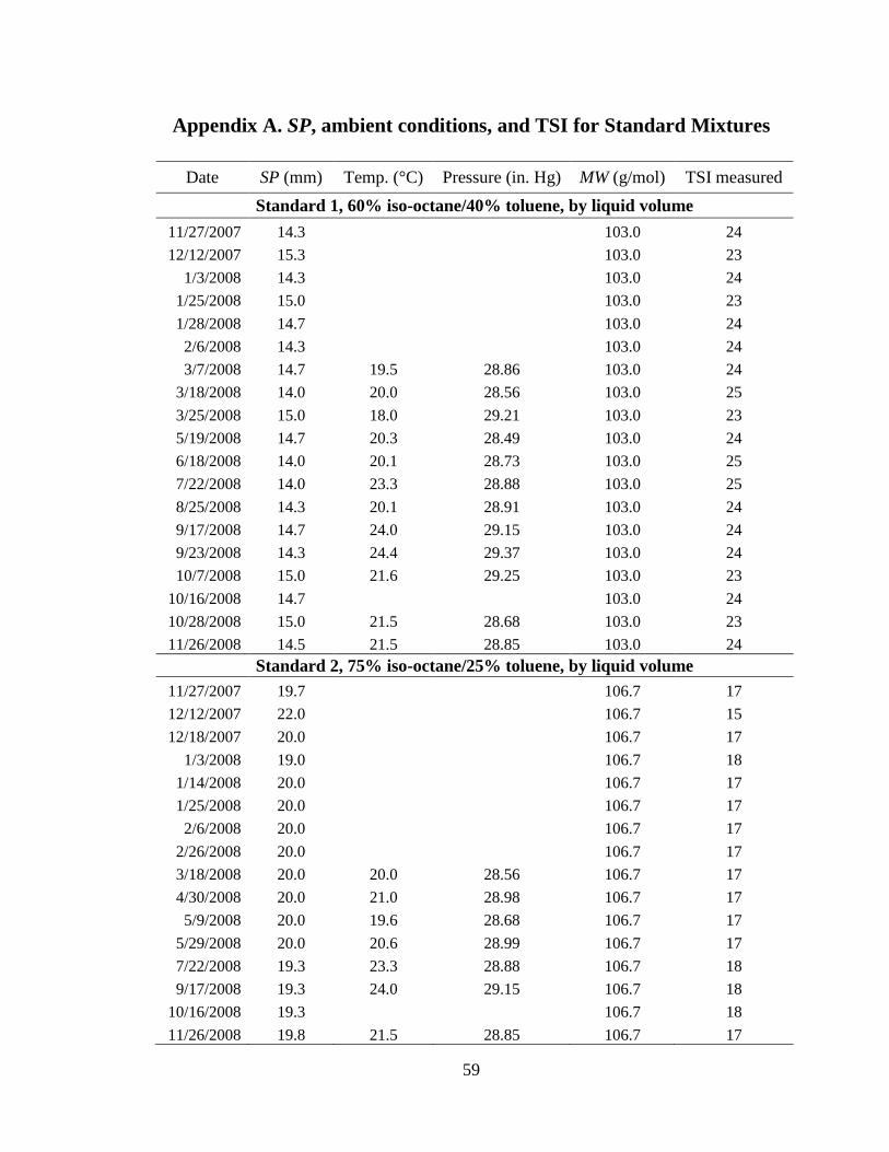
59

Appendix A. SP, ambient conditions, and TSI for Standard Mixtures

Date SP (mm) Temp. (°C) Pressure (in. Hg) MW (g/mol) TSI measured

Standard 1, 60% iso-octane/40% toluene, by liquid volume

11/27/2007 14.3

103.0 24

12/12/2007 15.3

103.0 23

1/3/2008 14.3

103.0 24

1/25/2008 15.0

103.0 23

1/28/2008 14.7

103.0 24

2/6/2008 14.3

103.0 24

3/7/2008 14.7 19.5 28.86 103.0 24

3/18/2008 14.0 20.0 28.56 103.0 25

3/25/2008 15.0 18.0 29.21 103.0 23

5/19/2008 14.7 20.3 28.49 103.0 24

6/18/2008 14.0 20.1 28.73 103.0 25

7/22/2008 14.0 23.3 28.88 103.0 25

8/25/2008 14.3 20.1 28.91 103.0 24

9/17/2008 14.7 24.0 29.15 103.0 24

9/23/2008 14.3 24.4 29.37 103.0 24

10/7/2008 15.0 21.6 29.25 103.0 23

10/16/2008 14.7

103.0 24

10/28/2008 15.0 21.5 28.68 103.0 23

11/26/2008 14.5 21.5 28.85 103.0 24

Standard 2, 75% iso-octane/25% toluene, by liquid volume

11/27/2007 19.7

106.7 17

12/12/2007 22.0

106.7 15

12/18/2007 20.0

106.7 17

1/3/2008 19.0

106.7 18

1/14/2008 20.0

106.7 17

1/25/2008 20.0

106.7 17

2/6/2008 20.0

106.7 17

2/26/2008 20.0

106.7 17

3/18/2008 20.0 20.0 28.56 106.7 17

4/30/2008 20.0 21.0 28.98 106.7 17

5/9/2008 20.0 19.6 28.68 106.7 17

5/29/2008 20.0 20.6 28.99 106.7 17

7/22/2008 19.3 23.3 28.88 106.7 18

9/17/2008 19.3 24.0 29.15 106.7 18

10/16/2008 19.3

106.7 18

11/26/2008 19.8 21.5 28.85 106.7 17

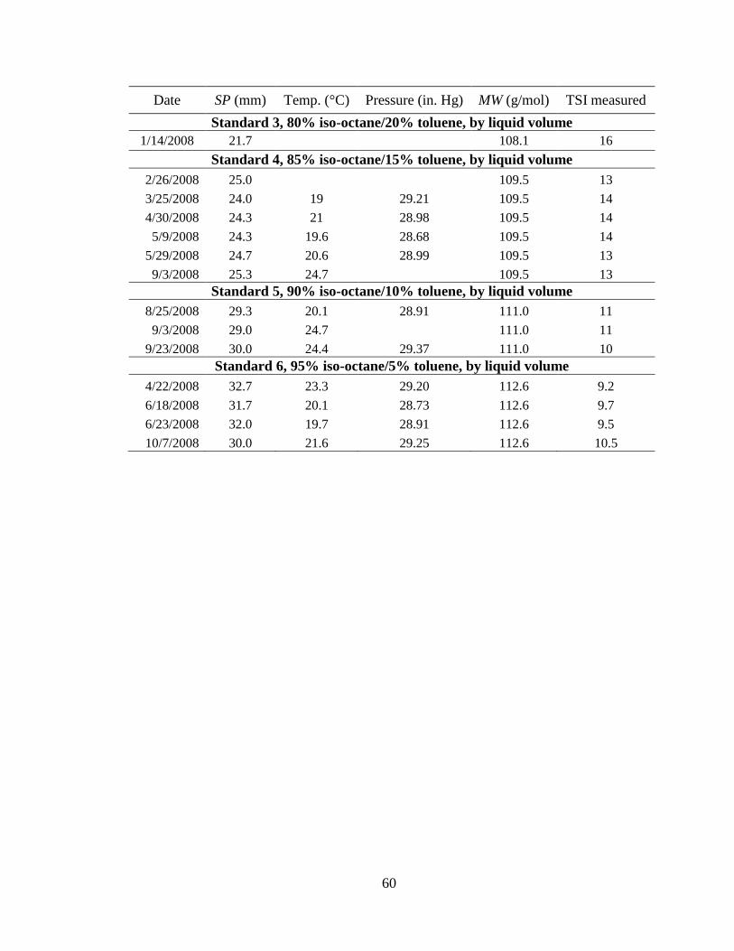
60

Date SP (mm) Temp. (°C) Pressure (in. Hg) MW (g/mol) TSI measured

Standard 3, 80% iso-octane/20% toluene, by liquid volume

1/14/2008 21.7

108.1 16

Standard 4, 85% iso-octane/15% toluene, by liquid volume

2/26/2008 25.0

109.5 13

3/25/2008 24.0 19 29.21 109.5 14

4/30/2008 24.3 21 28.98 109.5 14

5/9/2008 24.3 19.6 28.68 109.5 14

5/29/2008 24.7 20.6 28.99 109.5 13

9/3/2008 25.3 24.7

109.5 13

Standard 5, 90% iso-octane/10% toluene, by liquid volume

8/25/2008 29.3 20.1 28.91 111.0 11

9/3/2008 29.0 24.7

111.0 11

9/23/2008 30.0 24.4 29.37 111.0 10

Standard 6, 95% iso-octane/5% toluene, by liquid volume

4/22/2008 32.7 23.3 29.20 112.6 9.2

6/18/2008 31.7 20.1 28.73 112.6 9.7

6/23/2008 32.0 19.7 28.91 112.6 9.5

10/7/2008 30.0 21.6 29.25 112.6 10.5

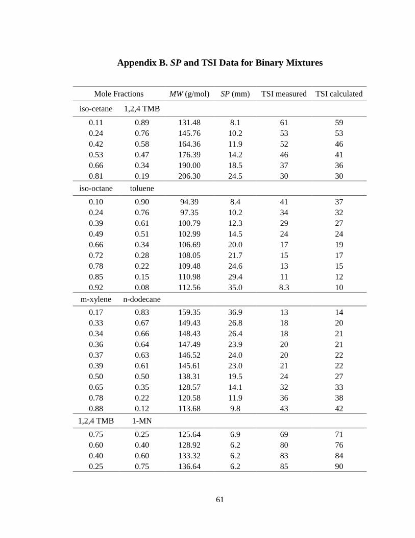
61

Appendix B. SP and TSI Data for Binary Mixtures

Mole Fractions MW (g/mol) SP (mm) TSI measured TSI calculated

iso-cetane 1,2,4 TMB

0.11 0.89 131.48 8.1 61 59

0.24 0.76 145.76 10.2 53 53

0.42 0.58 164.36 11.9 52 46

0.53 0.47 176.39 14.2 46 41

0.66 0.34 190.00 18.5 37 36

0.81 0.19 206.30 24.5 30 30

iso-octane toluene

0.10 0.90 94.39 8.4 41 37

0.24 0.76 97.35 10.2 34 32

0.39 0.61 100.79 12.3 29 27

0.49 0.51 102.99 14.5 24 24

0.66 0.34 106.69 20.0 17 19

0.72 0.28 108.05 21.7 15 17

0.78 0.22 109.48 24.6 13 15

0.85 0.15 110.98 29.4 11 12

0.92 0.08 112.56 35.0 8.3 10

m-xylene n-dodecane

0.17 0.83 159.35 36.9 13 14

0.33 0.67 149.43 26.8 18 20

0.34 0.66 148.43 26.4 18 21

0.36 0.64 147.49 23.9 20 21

0.37 0.63 146.52 24.0 20 22

0.39 0.61 145.61 23.0 21 22

0.50 0.50 138.31 19.5 24 27

0.65 0.35 128.57 14.1 32 33

0.78 0.22 120.58 11.9 36 38

0.88 0.12 113.68 9.8 43 42

1,2,4 TMB 1-MN

0.75 0.25 125.64 6.9 69 71

0.60 0.40 128.92 6.2 80 76

0.40 0.60 133.32 6.2 83 84

0.25 0.75 136.64 6.2 85 90

62

Mole Fractions MW (g/mol) SP (mm) TSI measured TSI calculated

decalin 1-MN

0.95 0.05 138.47 20.0 23 26

0.89 0.11 138.69 17.4 28 31

0.78 0.22 139.12 13.3 38 39

0.68 0.32 139.53 11.3 46 47

0.52 0.48 140.15 9.2 57 59

0.32 0.68 140.94 7.2 75 75

0.13 0.87 141.67 6.1 89 90

MCH 1-MN

0.98 0.02 99.20 29.9 8.7 8.6

0.95 0.05 100.24 23.7 12 11

0.91 0.09 102.31 18.9 17 15

0.81 0.19 106.39 14.7 25 24

0.72 0.28 110.54 11.5 34 33

0.62 0.38 114.82 10.5 40 42

0.42 0.58 123.83 7.3 64 61

0.21 0.79 132.85 6.3 81 80