A study on the pressure variation in a ducted heat exchanger using CFD

1 A study on the pressure variation in a ducted heat exchanger using CFD, UNSW@ADFA

A study on the pressure variation in a ducted heat

exchanger using CFD

Amresh Gyanathan1

University of New South Wales at the Australian Defence Force Academy

Effective cooling system design is important in the endurance event of the FSAE-A

competition. Research into sidepod design and radiator fan optimisation requires further

attention. To provide a further understanding on the aerodynamic effects of a sidepod

two investigations were performed using CFD. The first investigation identified that high

turbulence intensity levels created more uncertainty in predicting the radiator pressure

drops. Velocity of the airflow vary around bends in the sidepod. The airflow is

accelerated around the convex corners and decelerated around the concave corners.

Turbulence levels dissipate slower around convex corners. The deviation of radiator

pressure drops obtained using CFD from MUR's experimental results was more

significant if inlet flows were more turbulent. The second investigation illustrated that

high degrees of curvature in a sidepod may lead to internal flow separation. The latter

will occur if the diameter of curvature is too small or the separation length is too large.

Validating using data obtained from MUR may not be comprehensive, hence, raising the

importance for experimental testing to validate CFD results. RNG k-ε model proved its

resilience in all cases simulated. This thesis forms the foundation for future research and

design of sidepods in FSAE cars.

Contents

I. Introduction 2

II. Background Information 2

A. Contribution to cooling system design 2

B. Sidepod and radiator flowfield discussion 3

C. Heat exchanger modelling in FLUENT 4

D. Turbulence modelling in FLUENT 4

III. Methodology 5

A. Effects of inlet turbulence 5

B. Effects of varying curvature 5

IV. Results 6



V. Modification & further results 7



VI. Verification & validation of results 9



VII. Extension to current work 11

VIII. Conclusion 11

Acknowledgements 12

References 12

Nomenclature FSAE-A = Formula Society of Automotive Engineers-Australasia

1 LTA (RSAF), School of Engineering & Information Technology. ZEIT4500/4501.


CFD = Computational Fluid Dynamics

CAD = Computer Aided Design

OEM = Original Equipment Manufacturers

MUR = Melbourne University Racing

RNG = Renormalized Group

FVM = Finite Volume Method

kL = Pressure loss coefficient

1/α = Viscous inertial resistance factor

C2 = Inertial resistance factor

I. Introduction The FSAE-A competition is organised annually for all competing universities in the Australasia region. The

Academy Racing team is a regular participant of this competition. In this competition there are several events

that allow judges to assess and rank teams accordingly. The endurance event is assessed by pushing the car to its

limits by surviving 34 laps of the autocross track. This event forms 35% of the overall score and is of paramount

importance for all competitive teams [1]. In the 2010 FSAE-A competition the Academy Racing team placed

7th overall and 8th in the endurance event [2]. To improve this score, further design considerations can be

implemented into improving the cooling system of the car. In the FSAE-A competition in 2010, cost

optimization of the cooling system was part of the cost judging criteria. This was included in the combined score

awarded to the participating teams. In the 2010 FSAE-A competition, Academy Racing's WS10 car achieved a

score of 71.2 out of 100 [2]. This result can also be further improved upon. Thus, improving the cooling system

design will be necessary to perform better at subsequent FSAE-A competitions. This project aims to provide an

understanding into the aerodynamic considerations associated with sidepod flows, thus, contributing in part to

the overall cooling system design for the Academy Racing team's car.

II. Background Information

A. Contribution to cooling system design

In a FSAE cooling system design, three main aspects are usually considered. The first aspect is identifying

the heat loss and generation coefficients for each component in the cooling system and integrating them in a

heating circuit. The rate of heat generation and loss of various components in the cooling system have to be

studied along with the coolant flow rates under different conditions. Test driving under adverse atmospheric and

lap conditions may be conducted to give a worst-case scenario that accounts for factors such as slipstream of

leading cars, enforced slow running at high engine power, etc. This test drive will provide the measurements for

a thermally stable lap of the race-circuit, whereby total engine heat generated in one lap is equal to the total heat

dissipated by the radiator in that same lap.

The second aspect is to study the heat transfer characteristics of the radiator. This has to be done by both

experimental testing and CFD analysis for more complex experimental procedures. data obtained from the

former will be used to validate the latter. Coolant of various operating temperatures, pressures and velocities are

also modelled to identify the heat transfer characteristics of the radiator.

The third aspect is the integration of a radiator into a duct and testing the aerodynamic performance of it.

The design of the duct will factor in considerations such as varying cross-section areas throughout the duct,

varying degrees of curvature of the duct, varying inlet and outlet sizes and their locations with respect to the

aerodynamic interaction with the rest of the car. Test data can be used to validate the CFD analysis of this

ducted flow. In motorsport, such ducts are often termed as sidepods and are either situated front-on (ram air

ducted) or side-on (side air ducted) [3]. This project produces an end state that contributes towards the design of

an FSAE cooling system. It should be noted that such a contribution is made in part of the aerodynamic study of

ducted heat exchanger flows; one of the aspects of the FSAE cooling system design.

B. Sidepod and radiator flowfield discussion

The FSAE car is a racing car of a rear engine design. As such, the best ways to fit the radiator with the rest

of the car would be to have it mounted above the engine or in front of the engine. However, having the radiator

at these two locations comes with severe disadvantages. For a radiator situated above the engine, there is an

absence of consistent flow of air through the radiator as the region just above the engine has negligible airflow

(dead-air). This results in ineffective heat dissipation by the radiator. Furthermore, if the radiator is located at

the front of the engine (i.e. side of car or front of car), the acceleration and deceleration of the car will disrupt

the flow in the cooling ducts, thus, making it more intermittent. This is due to the inertia of the moving coolant


failing to accelerate or decelerate in time. This leads to other problems associated with intermittent pipe flows

(e.g. cavitation of coolant, coolant backflow, etc.). Sidepods are designed to overcome these problems. The

design of sidepods will be able to provide a dedicated air intake for heat dissipation of the radiator [4].

Radiator efficiency is affected by the pressure variation across it. This is in turn determined by the velocity

of the airflow through it. The sidepod has an overall pressure difference between the ends (i.e. inlet and outlet).

This pressure difference varies during different external flow conditions. If there is a pressure drop large enough

across the sidepod, then there will be a flow velocity through the radiator that maximises its heat dissipation. If

the pressure difference across the sidepod is not large enough, there will be inadequate airflow through the

radiator. To overcome this, a radiator fan can be modelled to provide the necessary airflow through the radiator

in all stages of operation. The radiator fan provides the necessary driving force by creating a pressure gradient

that pushes or pulls airflow through the radiator even in adverse situations. [5] states that equation 1 can be used

to compute the pressure drop across the radiator solely by considering the pressure loss coefficient, kL, and

normal airflow velocity on radiator surface, v.

(1)

It is found that a large kL value and a large increase in airflow velocity from the inlet of the sidepod to the

plane surface of the radiator produce the best cooling performance [6]. The latter can be achieved by intelligent

optimisation of the sidepod geometry by creating regions that speed up the airflow. [6] also states that the inlet

of the sidepod should not be made to be of a converging nature. This is to prevent the generation of backflow

and vortices upstream of the sidepod and flow separation on the exterior near the inlet of the sidepod. The speed

of natural airflow at the inlet of the sidepod is limited by the velocity of the race car along the autocross track. In

a typical track, the front velocity of the car is not expected to exceed 100 km/h, owing to the lack of straights in

the track [7]. As such the airflow at the inlet of the sidepod does not exceed 30 m/s, and hence, is

incompressible. This allows for commonly known equations (i.e. steady flows, Bernoulli’s equation &

continuity equation) to be used and model the airflow of a FSAE sidepod.

Sidepods often have varying degrees of curvature and cross-section areas to allow for optimised airflow

through the radiators. By varying the inlet, duct and outlet geometries of the sidepod, the internal airflow can be

studied and used to a design engineer’s advantage [5]. To achieve best cooling performance, a higher air mass

flow rate into the sidepod has to be obtained. However, from the perspective of vehicle aerodynamic drag, a

minimum amount of airflow should be diverted from the main flowfield around the car into the sidepod [8]. [8]

also mentions that considerations have to be made for outlet geometries of sidepods to prevent the loss of

downforce on the car. Outlet airflow design should also be considered as this airflow must not increase the

pressure of the low pressure region underneath the car to an unacceptable level.

The free-stream natural airflow entering a FSAE car sidepod is disturbed by several effects. One of them is

the turbulence generated from the rotation of the front wheels. The front wheels of the car of the Academy

Racing team are situated just to the front of the inlet of the sidepod. The effect of a rotating wheel on the inlet

turbulence of a side-pod varies with the velocity at which the free stream airflow is acting on the rotating wheel

[9]. This leads to a variety of inlet turbulence generation at the inlet. This can be modelled in ANSYS FLUENT

and further details can be found in the turbulence modelling section.

C. Heat exchanger modelling in FLUENT

The Academy Racing team uses a Borland Racing radiator used previously in the Formula Ford race cars.

No data for this radiator or other similar types of radiators within the same class could be obtained readily from

OEM. This means the only way to obtain heat transfer and pressure loss coefficients would be from the

experimental testing of the Borland radiator. From this testing, we can identify the pressure loss coefficient, kL,

and heat loss coefficient, h. Using equation 1, the pressure variation can then be estimated for a variety of

velocities. A quadratic curve of best fit can then be used to model the pressure variation distribution to be

analysed for porous media parameters. Section 7.2.3.6.11 of the ANSYS FLUENT user guide recommends the

use of two equations, 7-2 and 7-25 of the user guide (reflected here as equations 2 and 3 respectively) [10].

These two equations, when combined, culminate in equation 4. In these equations, Si represents the momentum

source term, Δn represents the radiator thickness, represents the viscous inertial resistance factor and C2 is

the inertial resistance factor. The coefficients found from the quadratic curve of best fit can now be used to find

and C2, which are used as inputs for the porous media region.

(

| | ) (2)

(3)


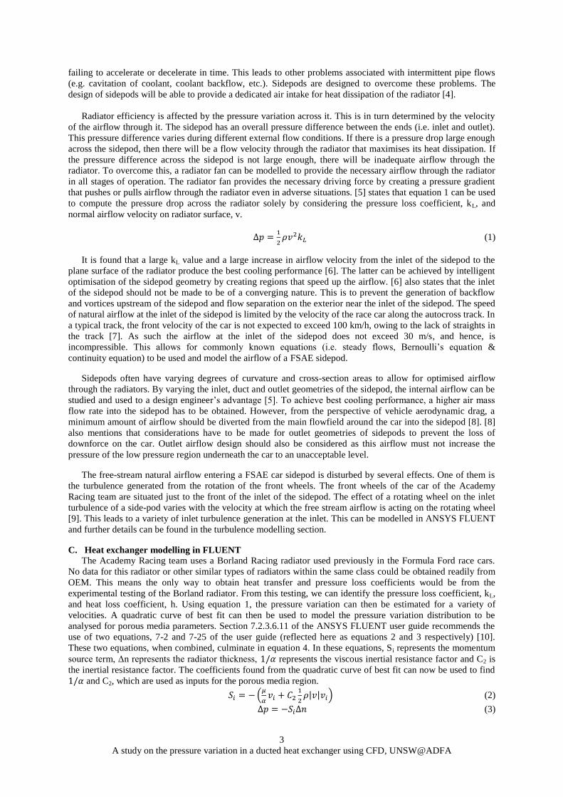
Figure 1. Fourth order

polynomial fit for kL from

MUR.

Figure 2. Extrapolation

of polynomial.

Figure 3. Power-law model

for kL versus velocity

showing conformal to trend

obtained from experimental

results.

Figure 4. Plot of

quadratic curve of best-fit

using cftool function in

MATLAB.

(

| | ) (4)

The FSAE team from MUR has performed experimental testing on their car radiator (similar class of

radiators) and have obtained a fourth-order polynomial fit for their results as shown in figure 1 [6]. Seeing that

the operating range of a FSAE race car exceeds a forward velocity of 5 m/s, This polynomial fit was then

compared for a larger velocity range to ensure that it would follow a similar trend to the experimental results.

This extrapolation of kL is found in figure 2.

From figure 2, it can be seen clearly that for

velocities after 6 m/s the fourth-order

polynomial fit does not follow a similar trend

as the experimental results. In order to obtain

a curve of best-fit that adheres to the trend of

the experimental data, a power-law model

was used. This model is found in equation 5.

This was substituted into equation 1 and a

series of loss coefficient values, kL, were

plotted against the normal velocity. These

values

(5)

(6)

allowed for a quadratic curve-fit to be used

and this is expressed in equation 6. This

quadratic expression is modelled to a 95%

confidence level using a MATLAB function

called cftool. The coefficients of equations 6

were then compared with those obtained from

equation 4 to find and C2, which will

then be used as the porous media inputs. This

comes from assuming that the radiator is

fitted tightly around the walls of the sidepod,

such that all airflow must flow through the

radiator, that the operating pressure was

assumed to be at 101 325Pa (1 standard

atmosphere) and that kL observed the same

trend for all velocities. Figure 3 shows the

power law approximation of kL versus velocity, while figure 4 shows how p is modelled via the cftool

function.

D. Turbulence modelling in FLUENT

The surroundings of the sidepod is exposed to turbulent

flows. Turbulence intensity captures the level of turbulence

in such flows. It represents the ratio of the root-mean-

square of velocity fluctuations to the mean flow velocity

[11]. Airflow through a FSAE car sidepod resemble that of

a low speed flow through large pipes. As such, the

turbulence intensity of such a flow normally does not

exceed 5% [12]. Additional consideration should also be

made for the external turbulence generated by the front

wheels and ground effects around the sidepod inlet when

performing CFD analysis. Sidepods have varying degrees

of curvature depending on the design requirements. As

such, a turbulence model that is most suitable for high

curvature flows is chosen. The RNG k-ε model was found

to be most suitable for such flows [13]. Despite the

effectiveness of the RNG k-ε model for high curvature

flows, a backup model will be considered as a precaution

when the former fails to provide a solution that converges

to an acceptable value. It is also recommended that the realizable k-ε model is more resilient for flows

undergoing high mathematical constraints [14][15]. This model will be used when the RNG k-ε model fails.

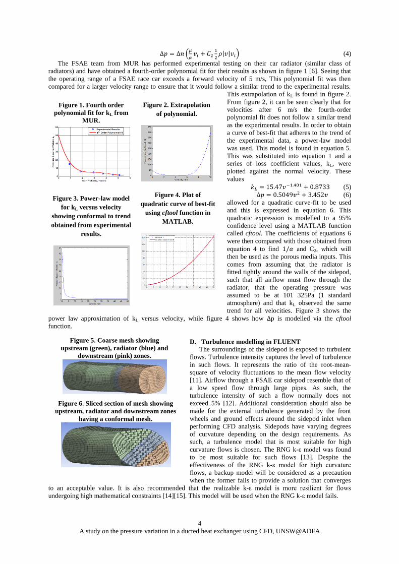
Figure 5. Coarse mesh showing

upstream (green), radiator (blue) and

downstream (pink) zones.

Figure 6. Sliced section of mesh showing

upstream, radiator and downstream zones

having a conformal mesh.


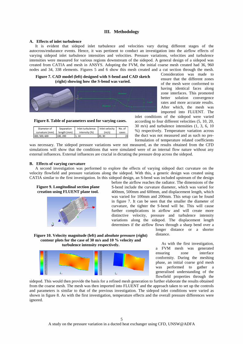
Figure 10. Velocity magnitude (left) and absolute pressure (right)

contour plots for the case of 30 m/s and 10 % velocity and

turbulence intensity respectively.

III. Methodology

A. Effects of inlet turbulence

It is evident that sidepod inlet turbulence and velocities vary during different stages of the

autocross/endurance events. Hence, it was pertinent to conduct an investigation into the airflow effects of

varying sidepod inlet turbulence intensities and velocities. Pressure variations, velocities and turbulence

intensities were measured for various regions downstream of the sidepod. A general design of a sidepod was

created from CATIA and mesh in ANSYS. Adopting the FVM, the initial coarse mesh created had 36, 960

nodes and 34, 338 elements. Figures 5 and 6 show this mesh created and a cut section through the mesh.

Consideration was made to

ensure that the different zones

of the mesh were conformed to

having identical faces along

zone interfaces. This promoted

better solution convergence

rates and more accurate results.

After which, the mesh was

imported into FLUENT. The

inlet conditions of the sidepod were varied

according to four different velocities (5, 10, 20,

30 m/s) and turbulence intensities (1, 3, 6, 10

%) respectively. Temperature variation across

the duct was not measured and as such no pre-

formulation of temperature related coefficients

was necessary. The sidepod pressure variations were not measured, as the results obtained from the CFD

simulations will show that the conditions that were simulated were of an internal flow nature without any

external influences. External influences are crucial in dictating the pressure drop across the sidepod.

B. Effects of varying curvature A second investigation was performed to explore the effects of varying sidepod duct curvature on the

velocity flowfield and pressure variations along the sidepod. With this, a generic design was created using

CATIA similar to the first investigation. In this sidepod design, an S-bend was included upstream of the design

before the airflow reaches the radiator. The dimensions of the

S-bend include the curvature diameter, which was varied for

400mm, 500mm and 600mm, and displacement length, which

was varied for 100mm and 200mm. This setup can be found

in figure 7. It can be seen that the smaller the diameter of

curvature, the tighter the S-bend will be. This will cause

further complications in airflow and will create more

distinctive velocity, pressure and turbulence intensity

variations along the sidepod. The displacement length

determines if the airflow flows through a sharp bend over a

longer distance or a shorter

distance.

As with the first investigation,

a FVM mesh was generated

ensuring zone interface

conformity. During the meshing

phase, an initial coarse grid mesh

was performed to gather a

generalised understanding of the

flowfield properties through the

sidepod. This would then provide the basis for a refined mesh generation to further elaborate the results obtained

from the coarse mesh. The mesh was then imported into FLUENT and the approach taken to set up the controls

and parameters is similar to that of the previous investigation. The sidepod inlet conditions were varied as

shown in figure 8. As with the first investigation, temperature effects and the overall pressure differences were

ignored.

Figure 9. Longitudinal section plane

creation using FLUENT plane tool.

Diameter

Diameter

Length

Figure 7. CAD model (left) designed with S-bend and CAD sketch

(right) showing how the S-bend was varied.

400, 500, 600 100, 200 1, 10 20, 30 24

No. of

cases

Diameter of

curvature (mm)

Separation

length (mm)

Inlet turbulence

intensity (%)

Inlet velocity

(m/s)

Figure 8. Table of parameters used for varying cases.


Figure 11. Turbulence intensity contour plots at different

locations of the sidepod. Sidepod outlet (left-most), radiator

outlet (2nd

from the left), radiator inlet (3rd

), cross-section plane

at bend (2nd

from the right) and sidepod inlet (right-most) are

reflected. The convex corner of the cross-section plane is

located at the bottom, while the concave corner is located on

top.

Figure 14. Turbulence intensity contour plots along

longitudinal sections at 10% inlet turbulence intensity and

30m/s inlet velocity. Top left plot is for the case of D=400mm,

L=200mm; bottom left is for the case of D=400mm,

L=100mm; top right is for the case of D=500mm, L=200mm;

and bottom right is for the case of D=600mm, L=200mm.

IV. Results

A. Effects of inlet turbulence.

Upon compiling the results of the simulations, the absolute pressure values were found to vary across the

entire cross-section. This comes about due to the presence of velocity changes throughout the interior of the

sidepod. A longitudinal section was taken along the length of the sidepod and along the length of the cross-

section face. Figure 9 shows how this longitudinal section was created. Using this longitudinal section, contour

plots of velocity magnitudes and absolute

pressures were found. These are

expressed in figure 10. It can be seen in

figure 10 that the velocity increases

around the convex (inner) corners and

decreases around the concave (outer)

corners. This can be likened to a

meandering river where the flow of the

water is always fastest on the inside of a

bend owing to the path of least flow

resistance. Since the flow is

incompressible, simple Bernoulli’s

principle can be applied. This leads to a

lower static pressure in the regions of

higher velocities and vice versa. The

values of static pressure outweigh

those of dynamic pressure (a function

of the square of velocity) and hence,

this leads to the absolute pressure

contours as shown in figure 10. Figure

10 shows the contour plots for the

specific case of 30 m/s and 10% inlet

velocity and inlet turbulence intensity

respectively. This can be used to a

cooling system designer’s advantage

by re-orientating the radiator to

receive faster oncoming airflow across

most of the cross section. Moreover,

figure 10 shows insufficient grid

resolution near the boundary layer

region at the sidepod walls. This will

be rectified in the modifications

section where a refined grid mesh will

be used.

Figure 11 shows the turbulence

intensities at various cross-sections for

the case of 10% inlet turbulence

intensity and 30 m/s inlet velocity.

Using FLUENT plane tool, a cross-

section profile was created at the bend

closer to the radiator. Figure 11 also

incorporates this profile with that of

the sidepod inlet, radiator inlet,

radiator outlet and the sidepod outlet.

From this figure, the progressive

variation in turbulence intensities

downstream from the sidepod inlet can

be observed. From figure 11, it can be

found that the turbulence intensity

started off at 10% at the sidepod inlet.

By the time the flow reaches the cross-

section plane, it has dropped to a

Figure 12. Velocity contour plot for the cases of

curvature diameter=500mm, inlet velocity=30m/s,

turbulence intensity=10%.Left plot shows the case for

separation length=100mm, right plot shows for

separation length=200mm.

Figure 13. Velocity contour plots for the case of curvature

diameter=400mm, inlet turbulence intensity=10%, inlet

velocity=30m/s. Left plot shows the case of 100mm

separation length while the right plot shows the case for

the 200mm separation length.


maximum of 8% and a minimum of 6.5%. These values continually decrease across the radiator and through the

aft section behind the radiator component. It is also observed that there is a higher value of turbulence intensity

closer to the concave corner (i.e. the region of lower velocity). This also means that the regions of higher

velocities have a lower value of turbulence intensity. In a sidepod, the radiator can be aligned to receive a higher

velocity flow rate and lower turbulence intensities. It has also become evident that the turbulence dissipation

rate nearer to the walls is much greater than

further away from the walls as shown in figure

11.

B. Effects of varying curvature.

The velocity contour plot for specific cases

are shown in figure 12. In this figure, for the

case of the longer S-bend separation length, we

can see that a larger proportion of the airflow at

the concave corner closest to the radiator section

is coloured in blue. This increase in the thickness

of slow moving fluid could also be due to flow

separation from its streamlines. Figure 13 shows

how this effect is more pronounced with higher

degrees of curvature.

Taking a look at the turbulence intensity

levels along the longitudinal section of the

sidepod yields results that help prove the

existence of flow separation from its streamlines.

Figure 14 shows several cases in which it is

suspected that airflow separation occurs on the

second concave corner of the S-bend. Observing

all turbulence intensity results, it was found that

for a smaller curvature diameter in the S-bend it is easier to obtain airflow

separation in the second concave corner of the S-bend. This is because for a

smaller curvature diameter the maximum S-bend separation length before

airflow separation occurs is reduced, as a smaller curvature diameter leads to a

tighter bend. The maximum S-bend separation length will prove to be useful in

the conceptual design process of the cooling system in a FSAE competition car.

Furthermore, the turbulence intensities for all cases are found to be higher and

more resilient along convex corners. This is proven in the first corner of the S-

bend that the airflow negotiates around for all cases. However, it must be noted

that these levels of turbulence intensities are mild in comparison to those of the

flow separation nature.

Paying closer attention to the inlet edges on all

cases reflected in figure 14, there is a spike in the

turbulence intensity levels. This can be attributed to

the design of the sidepod geometry to resemble a

curved fillet at the inlet edge. This has caused the

cross-section area to be converging to a minor extent,

thus causing small scale turbulence forming as

vortices [8]. The sensitivity of these vortices can be

seen here on a small extent; however, this may have

more serious consequences if the inlet cross-section

area converges to a greater extent. This should also

be an important consideration in cooling system

design.

V. Modifications & Further Results


Modifications were made to the coarse mesh to enable a more accurate modelling of fluid properties at the

near wall regions. A refined grid mesh was then created with 134, 595 nodes and 316, 569 elements with

Coarse Refined

Geometry Elements Elements

D400 L100 115412 233799

D400 L200 109244 343505

D500 L100 108934 354640

D500 L200 107037 211635

D600 L100 109306 213777

D600 L200 122460 220663

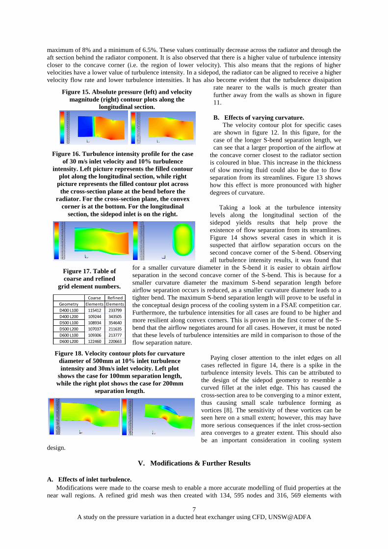
Figure 17. Table of

coarse and refined

grid element numbers.

Figure 15. Absolute pressure (left) and velocity

magnitude (right) contour plots along the

longitudinal section.

Figure 16. Turbulence intensity profile for the case

of 30 m/s inlet velocity and 10% turbulence

intensity. Left picture represents the filled contour

plot along the longitudinal section, while right

picture represents the filled contour plot across

the cross-section plane at the bend before the

radiator. For the cross-section plane, the convex

corner is at the bottom. For the longitudinal

section, the sidepod inlet is on the right.

Figure 18. Velocity contour plots for curvature

diameter of 500mm at 10% inlet turbulence

intensity and 30m/s inlet velocity. Left plot

shows the case for 100mm separation length,

while the right plot shows the case for 200mm

separation length.


inflation at the near wall regions of

the mesh. Figure 15 produces the

absolute pressure and velocity

magnitude variations along the

longitudinal section of the

sidepod. The velocity magnitude

profile shows a much smaller

boundary layer thickness than that

in figure 10. This proves that the

refined mesh resolved the solution

at the near wall regions to a good

level. Similar trends are observed

in figures 10 and 15,

where the velocity of

the airflow is greater

and the absolute

pressure is lower at the

convex corners and

vice versa.

Figure 16 shows

the variation of

turbulence intensity

along the longitudinal

section and the cross-

section at the corner

closest to the radiator.

This general variation

is similar to that

obtained for the coarse

mesh in figure 11.

However, it must be

noted that the turbulence intensities at the boundary layer of the regions varies slightly when compared to figure

11. Figure 16 depicts a more accurate solution where the turbulence region of influence affected by the

boundary layer is of a smaller proportion of the overall cross-section of the sidepod. Furthermore, from the

longitudinal section contour plot of turbulence intensity, it can be found that the convex corners of bends seem

to reduce the dissipation rate of turbulence as the turbulence intensities appear to be more resilient in the two

convex corners of the sidepod. This means that if the cooling system designer orientates the radiator to receive a

higher velocity flow rate in this specific sidepod geometry, then the radiator will also be subjected to more

inconsistent pressure drops across it due to the lower turbulence dissipation. Further optimisation studies can be

conducted to discover the right levels of turbulence that is acceptable for efficient radiator performance.

B. Effects of varying curvature.

The mesh created was inflated around the wall regions to ensure sufficient grid resolution to reflect these

modifications. Figure 17 shows the coarse and refined mesh grid elements. This shows how well resolved the

refined grid is.

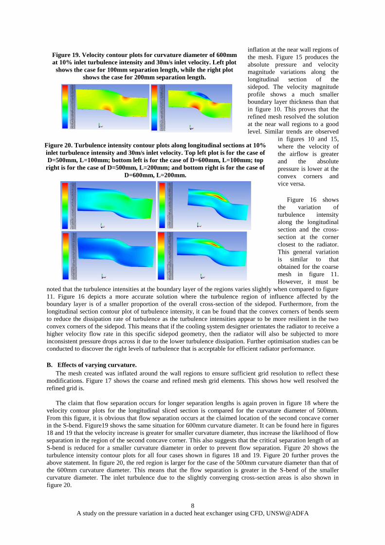
The claim that flow separation occurs for longer separation lengths is again proven in figure 18 where the

velocity contour plots for the longitudinal sliced section is compared for the curvature diameter of 500mm.

From this figure, it is obvious that flow separation occurs at the claimed location of the second concave corner

in the S-bend. Figure19 shows the same situation for 600mm curvature diameter. It can be found here in figures

18 and 19 that the velocity increase is greater for smaller curvature diameter, thus increase the likelihood of flow

separation in the region of the second concave corner. This also suggests that the critical separation length of an

S-bend is reduced for a smaller curvature diameter in order to prevent flow separation. Figure 20 shows the

turbulence intensity contour plots for all four cases shown in figures 18 and 19. Figure 20 further proves the

above statement. In figure 20, the red region is larger for the case of the 500mm curvature diameter than that of

the 600mm curvature diameter. This means that the flow separation is greater in the S-bend of the smaller

curvature diameter. The inlet turbulence due to the slightly converging cross-section areas is also shown in

figure 20.

Figure 19. Velocity contour plots for curvature diameter of 600mm

at 10% inlet turbulence intensity and 30m/s inlet velocity. Left plot

shows the case for 100mm separation length, while the right plot

shows the case for 200mm separation length.

Figure 20. Turbulence intensity contour plots along longitudinal sections at 10%

inlet turbulence intensity and 30m/s inlet velocity. Top left plot is for the case of

D=500mm, L=100mm; bottom left is for the case of D=600mm, L=100mm; top

right is for the case of D=500mm, L=200mm; and bottom right is for the case of

D=600mm, L=200mm.


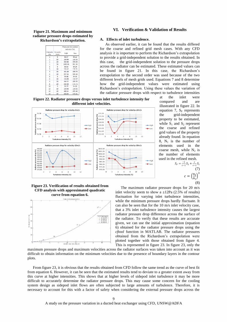
Figure 22. Radiator pressure drops versus inlet turbulence intensity for

different inlet velocities.

Figure 21. Maximum and minimum

radiator pressure drops estimated by

Richardson’s extrapolation.

VI. Verification & Validation of Results


As observed earlier, it can be found that the results differed

for the coarse and refined grid mesh cases. With any CFD

analysis it is important to perform the Richardson’s extrapolation

to provide a grid-independent solution to the results obtained. In

this case, the grid-independent solution to the pressure drops

across the radiator can be estimated. These estimated values can

be found in figure 21. In this case, the Richardson’s

extrapolation to the second order was used because of the two

different levels of mesh grids used. Equations 7 and 8 determine

how the grid-independent values were estimated using

Richardson’s extrapolation. Using these values the variation of

the radiator pressure drops with respect to turbulence intensities

at the inlet were

compared and are

illustrated in figure 22. In

equation 7, SF represents

the grid-independent

property to be estimated,

while S1 and S2 represent

the coarse and refined

grid values of the property

already found. In equation

8, N1 is the number of

elements used in the

coarse mesh, while N2 is

the number of elements

used in the refined mesh.

(7)

(

)

(8)

The maximum radiator pressure drops for 20 m/s

inlet velocity seem to show a ±12Pa (2.5% of results)

fluctuation for varying inlet turbulence intensities,

while the minimum pressure drops hardly fluctuate. It

can also be seen that for the 10 m/s inlet velocity case,

that a 3% inlet turbulence intensity causes the largest

radiator pressure drop difference across the surface of

the radiator. To verify that these results are accurate

given, we can use the initial approximation (equation

6) obtained for the radiator pressure drops using the

cftool function in MATLAB. The radiator pressures

obtained from the Richardson’s extrapolation were

plotted together with those obtained from figure 4.

This is represented in figure 23. In figure 23, only the

maximum pressure drops and maximum velocities across the radiator surfaces was taken into account as it was

difficult to obtain information on the minimum velocities due to the presence of boundary layers in the contour

plots.

From figure 23, it is obvious that the results obtained from CFD follow the same trend as the curve of best fit

from equation 6. However, it can be seen that the estimated results tend to deviate to a greater extent away from

this curve at higher intensities. This shows that at higher levels of sidepod inlet turbulence it may be more

difficult to accurately determine the radiator pressure drops. This may cause some concern for the cooling

system design as sidepod inlet flows are often subjected to large amounts of turbulence. Therefore, it is

necessary to account for this with a factor of safety when considering the external pressure drops across the

Figure 23. Verification of results obtained from

CFD analysis with approximated quadratic

curve from equation 6.


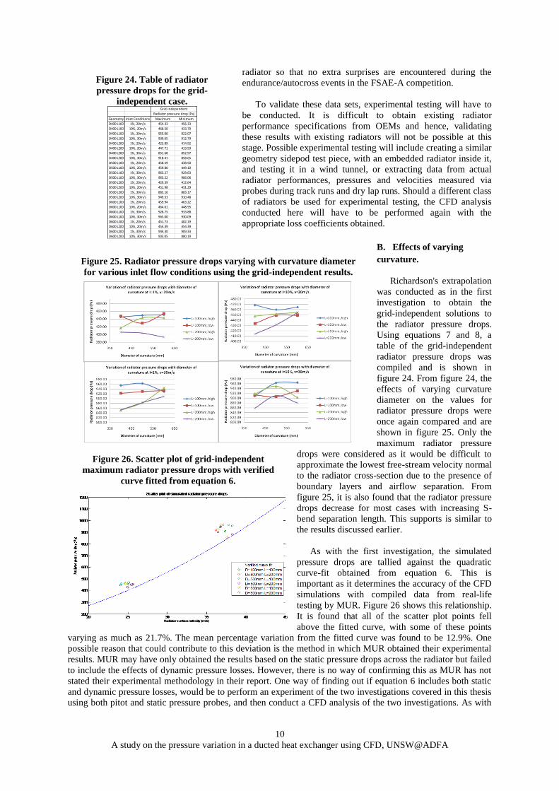
Figure 24. Table of radiator

pressure drops for the grid-

independent case.

Geometry Inlet Conditions Maximum Minimum

D400 L100 1%, 20m/s 454.33 456.33

D400 L100 10%, 20m/s 468.50 433.79

D400 L100 1%, 30m/s 955.00 922.07

D400 L100 10%, 30m/s 909.65 912.79

D400 L200 1%, 20m/s 425.89 414.92

D400 L200 10%, 20m/s 447.71 413.93

D400 L200 1%, 30m/s 851.68 852.97

D400 L200 10%, 30m/s 918.41 858.65

D500 L100 1%, 20m/s 458.59 438.50

D500 L100 10%, 20m/s 459.80 449.10

D500 L100 1%, 30m/s 963.27 929.63

D500 L100 10%, 30m/s 963.22 906.06

D500 L200 1%, 20m/s 429.39 412.64

D500 L200 10%, 20m/s 451.98 431.29

D500 L200 1%, 30m/s 883.16 883.17

D500 L200 10%, 30m/s 949.53 910.48

D600 L100 1%, 20m/s 459.94 463.22

D600 L100 10%, 20m/s 464.61 448.95

D600 L100 1%, 30m/s 928.75 933.88

D600 L100 10%, 30m/s 965.00 930.09

D600 L200 1%, 20m/s 451.73 402.19

D600 L200 10%, 20m/s 454.39 454.39

D600 L200 1%, 30m/s 944.30 909.33

D600 L200 10%, 30m/s 903.05 880.19

Grid-independent

Radiator pressure drop (Pa)

radiator so that no extra surprises are encountered during the

endurance/autocross events in the FSAE-A competition.

To validate these data sets, experimental testing will have to

be conducted. It is difficult to obtain existing radiator

performance specifications from OEMs and hence, validating

these results with existing radiators will not be possible at this

stage. Possible experimental testing will include creating a similar

geometry sidepod test piece, with an embedded radiator inside it,

and testing it in a wind tunnel, or extracting data from actual

radiator performances, pressures and velocities measured via

probes during track runs and dry lap runs. Should a different class

of radiators be used for experimental testing, the CFD analysis

conducted here will have to be performed again with the

appropriate loss coefficients obtained.

B. Effects of varying

curvature.

Richardson's extrapolation

was conducted as in the first

investigation to obtain the

grid-independent solutions to

the radiator pressure drops.

Using equations 7 and 8, a

table of the grid-independent

radiator pressure drops was

compiled and is shown in

figure 24. From figure 24, the

effects of varying curvature

diameter on the values for

radiator pressure drops were

once again compared and are

shown in figure 25. Only the

maximum radiator pressure

drops were considered as it would be difficult to

approximate the lowest free-stream velocity normal

to the radiator cross-section due to the presence of

boundary layers and airflow separation. From

figure 25, it is also found that the radiator pressure

drops decrease for most cases with increasing S-

bend separation length. This supports is similar to

the results discussed earlier.

As with the first investigation, the simulated

pressure drops are tallied against the quadratic

curve-fit obtained from equation 6. This is

important as it determines the accuracy of the CFD

simulations with compiled data from real-life

testing by MUR. Figure 26 shows this relationship.

It is found that all of the scatter plot points fell

above the fitted curve, with some of these points

varying as much as 21.7%. The mean percentage variation from the fitted curve was found to be 12.9%. One

possible reason that could contribute to this deviation is the method in which MUR obtained their experimental

results. MUR may have only obtained the results based on the static pressure drops across the radiator but failed

to include the effects of dynamic pressure losses. However, there is no way of confirming this as MUR has not

stated their experimental methodology in their report. One way of finding out if equation 6 includes both static

and dynamic pressure losses, would be to perform an experiment of the two investigations covered in this thesis

using both pitot and static pressure probes, and then conduct a CFD analysis of the two investigations. As with

Figure 25. Radiator pressure drops varying with curvature diameter

for various inlet flow conditions using the grid-independent results.

Figure 26. Scatter plot of grid-independent

maximum radiator pressure drops with verified

curve fitted from equation 6.


all CFD analyses, real-life validation is essential and hence, a full experimental procedure of this investigation is

recommended in order to completely validate the obtained CFD results.

VII. Extension of current work

It can be inferred that experimental validation is necessary to provide the real life data to check the fidelity

of CFD results. Without which, these results obtained cannot be confidently incorporated into the cooling

system design of the FSAE competition car. In order to conduct such experimental procedures, a wind tunnel

large enough to accommodate a scaled model sidepod is necessary to prevent the near-wall effects from

affecting the pressure and velocity results obtained. Moreover, careful consideration would have to be given as

to how much time the Academy Racing team can make do without the radiator component of their car. This

experimental procedure will have to be allocated to being conducted at times when the need for operating on the

car is low.

Apart from validating the two investigations performed in this thesis, a study into the effects of varying

outlet pressures should be included at both the experimental and CFD analytical levels. This is necessary as the

rotating wheels located just aft of the sidepod outlet causes extra interference and pressure variations that will

affect the pressure drops across the sidepod. In the CFD analysis component of this proposed project, a rotating

wheel can be modelled separately to understand the aerodynamic effects before using user defined functions to

model the sidepod outlet conditions. This will require extensive computational resources and hence, efficient

resource management is required.

It is proposed in this report that orientating the radiator at angle towards the oncoming airflow in a sidepod

with bends would be a wise option so as to obtain the fastest airflow velocities flowing across the radiator cross-

section. A CFD optimisation study can be performed to discover the best angle of orientation to maximise

radiator cooling efficiency. Once this optimisation study is completed, it can be validated by experimentally

testing the best angle of orientation for the radiator.

Finally, it is also proposed that the effects of external flowfields on the internal flows of the sidepod be

studied. The experimental part of this study can be performed by placing pressure and velocity probes around

the vicinity of the radiator and sidepod as the car is test driven around a specified circuit that encompasses

varying forward speeds, engine power outputs and parts of the race-track. In the CFD analysis component of this

study, user defined functions may be used to model the external, inlet and outlet airflows. This will allow the

cooling system designer to use a simulated wind/gust model to predict several instances during a race lap. The

designer would then be able to obtain sidepod pressure differences and compare them with the radiator pressure

drops simulated to calculate the required pressure rise required by a radiator fan. Careful consideration should

be made in the resource management of this project as highly extensive computational requirements will be

required.

VIII. Conclusion

After performing these two investigations, several issues have been brought to light. The prediction of flows

in a sidepod via CFD simulations becomes more difficult with greater turbulence intensity levels at the inlet and

outlet of the sidepods. This will lead to additional flow velocity perturbations that will either mildly speed up or

slow down the airflow on the radiator surface. Such variation in airflow velocities is often coupled with bends in

a sidepod. These bends will allow designers to completely exploit the increase in the velocity of normal airflow

on the radiator. Studying these bends is likened to that studying water flowing in a meandering river, and using

this analogy, designers can create the ideal bend with appropriate degrees of curvature to speed up slower

velocities as much as possible without causing flow separation in slower regions.

Turbulence intensities were identified to dissipate at a lower rate around convex corners and much faster

around concave corners. It was also observed that with increasing turbulence intensities at the sidepod inlet, the

deviation from experimentally derived data is more significant. For sidepods with an S-bend, it was found that

flow separation may occur if the curvature diameter becomes too small or the separation length is too large. If

the latter condition occurs, the pressure drop across the radiator will decrease. The resilience in the RNG k-ε

model was also seen in the two investigations where the realizable k-ε model was not required to be used in any

of the cases modelled. Experimental validation of the obtained results is crucial in assuring the designer that the

simulations had solved the right equations in the correct manner. Hitherto, there has been a lack of research into

sidepods for FSAE cars. Thus, this thesis will provide the groundwork for future research into sidepods and car

cooling system design for FSAE.


Acknowledgements The author of this thesis would like to thank several people who throughout the course of this project who

provided great support and advice, without which the author would not have been able to successfully complete

this thesis. The author would like to thank the thesis supervisor, Mr Alan Fien, for his undying support and

efforts in assisting the former to overcome his obstacles faced during the various phases of the project. Alan

had, on several occasions, sacrificed his spare time to assist the author with his problems. The author would also

like to thank independent advisor, Dr John Young, who provided great levels of guidance with the CFD

component of this project.

The author would also like to thank Dr Warren Smith, PLTOFFs Paul Gardner and Alistair Weir for their

insights into the requirements of the Academy Racing team. The author also wishes to thank his undergraduate

friends from Singapore who assisted in running simulations and extracting useful data for this project. Lastly,

the author wishes to thank the Academy Racing team members for providing a great working environment and a

lively atmosphere whilst working with them.

References

[1] About FSAE, Academy Racing website, http://www.fsae.unsw.adfa.edu.au/about.php, accessed 19 Oct 11.

[2] 2010 FSAE-A results, http://www.saea.com.au/wp-content/uploads/2011/09/2010-FSAE-A-Results.pdf, accessed 19 Oct

11.

[3] Milliken, W. F., Milliken, D. L., Race Car Vehicle Dynamics, SAE International Publishing, Twelfth edition, 1995,

p556.

[4] Hucho, W., Aerodynamics of Road Vehicles-From Fluid Mechanics to Vehicle Engineering, Butterworth & Co.

Publishers, p5, 1987.

[5] De Silva, C. M., Nor Azmi, M., Christie, T., Abou-Saba, E., Ooi, A., Computational Flow Modelling of Formula-SAE

Sidepods for Optimum Radiator Heat Management, Journal of Engineering Science and Technology, Vol 6, No. 1 (2011)

94-108 @ School of Engineering, Taylor’s University.

[6] Milliken, W. F., Milliken, D. L., Race Car Vehicle Dynamics, SAE International Publishing, Twelfth edition, 1995,

p558.

[7] Gardner, P. F., How fast does a FSAE race car travel in an autocross/endurance track?, Pers Comms, 7 Aug 2011.

[8] Adams, H., Chassis Engineering, HPBooks, published by the Berkley Publishing Group, 1993, pp102-103.

[9] Diasinos, S. The Aerodynamic Interaction of a Rotating Wheel and a Downforce Producing Wing in Ground Effect. PhD

thesis, School of Mechanical & Manufacturing Engineering, UNSW, March 2009.

[10] Section 7.2.3.6.11, Deriving the Porous Coefficients Based on Experimental Pressure and Velocity Data, Chapter 7:

Cell Zone and Boundary Conditions, ANSYS FLUENT user guide, Release 13.0.

[11] Chapter 6.2.2, Determining turbulence parameters, Fluent6.1 online help, http://jullio.pe.kr/fluent6.1/

help/html/ug/node178.htm, accessed 21 Oct 2011.

[12] Turbulence Intensity - Medium turbulence case, http://www.cfd-online.com/Wiki/Turbulence_intensity, accessed 15

Oct 2011.

[13] Ming, Y., Feng, S., Zhong, X., Renormalization Group Based k-ε Turbulence Model for Flows in a Duct with Strong

Curvature, International Journal of Engineering Science, Vol 34, No. 2, pp243-248, 1996.

[14] Chapter 4.3.3.1, Overview of Realizable k-e Model – FLUENT Theory Guide, pdf document, accessed 03 Oct 2011.

[15] Mossad, R., Yang, W., Schwarz, M. P., Numerical Prediction of Air Flow in a Sharp 90⁰ Elbow, Seventh Int. Conf. On

CFD in the Minerals and Process Industries, CSIRO, Melbourne, 9-11 December 2009.

Documents

A study on the pressure variation in a ducted heat exchanger using CFD