Embed Size (px)
Citation preview

A Study of White Dwarfs in the SolarNeighbourhood
Adela Kawka
This thesis is presented for the degree of Doctor of Philosophy of
Murdoch University.
2003

I declare that this thesis is my own account of my research and contains as its
main content work, which has not previously been submitted for a degree at any
tertiary education institution.
Adela Kawka

Abstract
The aim of this thesis is to revisit the properties of white dwarf stars in the Solar
neighbourhood (distance � 100 pc), in particular their magnetic fields, the occur-
rence of binarity and their space density. This thesis presents observations and
analysis of a sample of white dwarfs from the southern hemisphere. Over 80 ob-
jects were observed spectroscopically, and 65 of these were also observed with a
spectropolarimeter. Many of the white dwarfs observed belong to the Solar neigh-
bourhood, and can be used to study the star formation and evolution in this region.
Our spectropolarimetric measurements helped constrain the fraction of magnetic
white dwarfs in the Solar neighbourhood. Combining data from different surveys, I
found a higher fraction of these objects in the relatively old local population than in
other younger selections such as the Palomar-Green survey which suggests magnetic
field evolution in white dwarfs, or different sets of progenitors. The progenitors of
magnetic white dwarfs have been assumed to be Ap and Bp stars, however I find
that the properties and number of Ap and Bp stars would only explain white dwarfs
with magnetic fields larger than 100 MG. The number of known white dwarfs is
believed to be complete to about 13 pc, however the sample is certainly incomplete
to 20 pc from the Sun. To identify new white dwarfs in the Solar neighbourhood,
some possibly magnetic or in binaries, numerous candidate white dwarfs from the
Revised NLTT catalogue have been observed, which resulted in the discovery of 13
new white dwarfs, with 4 of these having a distance that places them within 20
pc of the Sun. The candidates were selected using a V − J reduced-proper-motion
diagram and optical-infrared diagram. A total of 417 white dwarf candidates were
selected, 200 of these have already been spectroscopically confirmed as white dwarfs.
Spectroscopic confirmation is required for the remaining 217 candidates, many of
these are likely to belong to the Solar neighbourhood. Four close binaries consisting

of a white dwarf and a cool companion were also observed, for which atmospheric
and orbital parameters were obtained. The photometry for two of these binary
systems, BPM 71214 and EC 13471-1258 shows that the secondary stars are filling
their Roche lobes, and combined with their orbital parameters, these systems are
very good candidates for hibernating novae. The time of their previous interaction
or the extent of this interaction are unknown. The two other binary systems, BPM
6502 and EUVE J0720-31.7 are post-common envelope binaries. BPM 6502 is not
expected to interact within a Hubble time, however EUVE J0720−31.7 is expected
to become a cataclysmic variable within a Hubble time. The atmospheric parame-
ters of the white dwarfs were determined using model atmosphere codes which were
modified for the present study to include convective energy transfer, self-broadening
and Lyman satellite features.

Contents
1 Introduction 1
1.1 Context . . . . . . . . . . . . . . . . . . . . . . . . . . . . . . . . . . 1
1.2 Magnetic white dwarfs . . . . . . . . . . . . . . . . . . . . . . . . . . 6
1.2.1 Properties of the Population . . . . . . . . . . . . . . . . . . . 6
1.2.2 Origin of Magnetic Fields in White Dwarfs . . . . . . . . . . . 8
1.3 Close Binary Systems . . . . . . . . . . . . . . . . . . . . . . . . . . . 11
1.3.1 Evolution . . . . . . . . . . . . . . . . . . . . . . . . . . . . . 12
1.3.2 Hibernating Novae . . . . . . . . . . . . . . . . . . . . . . . . 14
1.4 Overview of the thesis . . . . . . . . . . . . . . . . . . . . . . . . . . 18
2 Model Atmospheres 20
2.1 Basic principles . . . . . . . . . . . . . . . . . . . . . . . . . . . . . . 21
2.2 Convective Transfer . . . . . . . . . . . . . . . . . . . . . . . . . . . . 23
2.2.1 Convective instability . . . . . . . . . . . . . . . . . . . . . . . 24
2.2.2 Mixing length theory . . . . . . . . . . . . . . . . . . . . . . . 25
2.3 Opacities . . . . . . . . . . . . . . . . . . . . . . . . . . . . . . . . . . 33
2.3.1 Hydrogen line broadening . . . . . . . . . . . . . . . . . . . . 35
2.3.2 Total line absorption profile . . . . . . . . . . . . . . . . . . . 37
2.3.3 Combining all opacities . . . . . . . . . . . . . . . . . . . . . . 38
2.4 Synthetic spectra . . . . . . . . . . . . . . . . . . . . . . . . . . . . . 39
i

CONTENTS ii
3 Properties of Local White Dwarfs 49
3.1 Introduction . . . . . . . . . . . . . . . . . . . . . . . . . . . . . . . . 49
3.2 Techniques for Measuring Magnetic Fields . . . . . . . . . . . . . . . 51
3.2.1 Zeeman Spectroscopy . . . . . . . . . . . . . . . . . . . . . . . 51
3.2.2 Spectropolarimetry . . . . . . . . . . . . . . . . . . . . . . . . 53
3.3 Observations . . . . . . . . . . . . . . . . . . . . . . . . . . . . . . . . 55
3.3.1 Spectropolarimetry . . . . . . . . . . . . . . . . . . . . . . . . 55
3.3.2 Complementary Spectroscopy . . . . . . . . . . . . . . . . . . 56
3.3.3 Spectroscopy of NLTT Stars . . . . . . . . . . . . . . . . . . . 56
3.4 Analysis . . . . . . . . . . . . . . . . . . . . . . . . . . . . . . . . . . 58
3.4.1 Single White Dwarfs . . . . . . . . . . . . . . . . . . . . . . . 63
3.4.2 Ultramassive White Dwarfs . . . . . . . . . . . . . . . . . . . 68
3.4.3 Binary Stars . . . . . . . . . . . . . . . . . . . . . . . . . . . . 71
3.4.4 Non-DA Stars . . . . . . . . . . . . . . . . . . . . . . . . . . . 76
3.4.5 Discussion . . . . . . . . . . . . . . . . . . . . . . . . . . . . . 76
3.5 Origins of Magnetic White Dwarfs . . . . . . . . . . . . . . . . . . . . 78
3.6 Revisiting the local Population of White Dwarfs . . . . . . . . . . . . 84
3.6.1 New Local White Dwarfs . . . . . . . . . . . . . . . . . . . . . 88
3.6.2 Kinematics . . . . . . . . . . . . . . . . . . . . . . . . . . . . 114
3.6.3 Discussion . . . . . . . . . . . . . . . . . . . . . . . . . . . . . 120
3.7 Summary . . . . . . . . . . . . . . . . . . . . . . . . . . . . . . . . . 121
4 Close Binary Systems 122
4.1 Introduction . . . . . . . . . . . . . . . . . . . . . . . . . . . . . . . . 122
4.2 Measuring Orbital Parameters . . . . . . . . . . . . . . . . . . . . . . 124
4.3 Observations . . . . . . . . . . . . . . . . . . . . . . . . . . . . . . . . 127
4.3.1 Optical Spectroscopy and Photometry . . . . . . . . . . . . . 127
4.3.2 Archival Ultraviolet Data . . . . . . . . . . . . . . . . . . . . 130
4.4 Analysis . . . . . . . . . . . . . . . . . . . . . . . . . . . . . . . . . . 131

CONTENTS iii
4.4.1 BPM 71214 . . . . . . . . . . . . . . . . . . . . . . . . . . . . 131
4.4.2 EUVE J0720-31.7 . . . . . . . . . . . . . . . . . . . . . . . . . 144
4.4.3 BPM 6502 . . . . . . . . . . . . . . . . . . . . . . . . . . . . . 147
4.4.4 EC 13471-1258 . . . . . . . . . . . . . . . . . . . . . . . . . . 157
4.5 Summary . . . . . . . . . . . . . . . . . . . . . . . . . . . . . . . . . 171
5 Conclusion 174
5.1 Main Results . . . . . . . . . . . . . . . . . . . . . . . . . . . . . . . 174
5.2 Future Work . . . . . . . . . . . . . . . . . . . . . . . . . . . . . . . . 178
A Known Magnetic White Dwarfs 180
B Tables of Models 188
C Southern Spectropolarimetric Survey 207
D Spectroscopy of Local White Dwarfs 230
E Observations of Close Binary Systems 234
F White Dwarf Database 251
List of Figures
2.1 Fraction of convective energy transport for 7000 ≤ Teff ≤ 14000 K . . 34
2.2 Fraction of convective energy transport for 4500 ≤ Teff ≤ 6500 K . . 41
2.3 Temperature structure for models at 7000 ≤ Teff ≤ 14000 K . . . . . 42
2.4 Temperature structure for models at 4500 ≤ Teff ≤ 6500 K . . . . . . 43
2.5 Total gas pressure structure for models at 7000 ≤ Teff ≤ 14000 K . . 44
2.6 Total gas pressure structure for models at 4500 ≤ Teff ≤ 6500 K . . . 45
2.7 Synthetic spectra for Teff = 5000 to 14000 K . . . . . . . . . . . . . . 46
2.8 Synthetic spectra for Teff = 16000 to 84000 K . . . . . . . . . . . . . 47
2.9 Model line profiles of Hα to Hε . . . . . . . . . . . . . . . . . . . . . 48
3.1 Distribution of magnetic field measurements . . . . . . . . . . . . . . 59
3.2 Synthetic spectra simulations . . . . . . . . . . . . . . . . . . . . . . 62
3.3 Flux and circular polarization spectra of WD 0621−376, WD 2039−682,
WD 2105−820 and WD 2359−434 . . . . . . . . . . . . . . . . . . . . 65
3.4 Flux and circular polarization spectra of LB 9802 . . . . . . . . . . . 66
3.5 Flux and circular polarization spectra of EUVE J0823−25.4 . . . . . 73
3.6 Flux and circular polarization spectra of WD 2329−291 . . . . . . . . 77
3.7 The observed and predicted incidence of magnetism in white dwarfs . 83
3.8 Cumulative distributions of magnetic white dwarfs in the Solar neigh-
bourhood . . . . . . . . . . . . . . . . . . . . . . . . . . . . . . . . . 95
3.9 Spectrum of the DA plus dMe WD 1717−345 . . . . . . . . . . . . . 97
iv

LIST OF FIGURES v
3.10 Spectra of KUV 05097+1649, WD 0311−543 and WD 1013−559 com-
pared to an F5V spectrum . . . . . . . . . . . . . . . . . . . . . . . . 98
3.11 Balmer line profiles of GD 1212 . . . . . . . . . . . . . . . . . . . . . 99
3.12 Reduced Proper Motion and optical-infrared diagrams of NLTT stars 101
3.13 Spectra of observed DA white dwarfs . . . . . . . . . . . . . . . . . . 103
3.14 Spectra of new non-DA white dwarfs . . . . . . . . . . . . . . . . . . 104
3.15 Balmer line profiles of NLTT 529 . . . . . . . . . . . . . . . . . . . . 105
3.16 IUE spectrum of NLTT 31748 . . . . . . . . . . . . . . . . . . . . . . 106
3.17 Blamer line profiles of NLTT 31748 . . . . . . . . . . . . . . . . . . . 107
3.18 Spectrum of the DZ white dwarf NLTT 40607 . . . . . . . . . . . . . 108
3.19 Balmer line profiles of NLTT 49985 . . . . . . . . . . . . . . . . . . . 109
3.20 Balmer line profiles of NLTT 53177 . . . . . . . . . . . . . . . . . . . 110
3.21 Balmer line profiles of NLTT 53468 . . . . . . . . . . . . . . . . . . . 111
3.22 Blamer line profiles of NLTT 55932 . . . . . . . . . . . . . . . . . . . 112
3.23 Spectra of NLTT 8435, NLTT 8581, NLTT 58805 and LHS 1415 . . . 115
3.24 B − V and U − B photometry of observed local white dwarfs . . . . . 116
3.25 V − J and J − H photometry of observed local white dwarfs . . . . . 117
3.26 UV diagram of colour-selected rNLTT white dwarfs . . . . . . . . . . 119
4.1 Hα radial velocity curve and period analysis of BPM 71214 . . . . . . 132
4.2 Absorption radial velocity curve of BPM 71214 . . . . . . . . . . . . 133
4.3 Decomposed spectrum of BPM 71214 . . . . . . . . . . . . . . . . . . 135
4.4 Balmer line profiles of BPM 71214 . . . . . . . . . . . . . . . . . . . . 136
4.5 Light curve of BPM 71214 in the I band . . . . . . . . . . . . . . . . 139
4.6 Light curve of BPM 71214 in the R band . . . . . . . . . . . . . . . . 140
4.7 Hα radial velocity and equivalent width curves with their period anal-
yses . . . . . . . . . . . . . . . . . . . . . . . . . . . . . . . . . . . . 146
4.8 Balmer line profiles of EUVE J0720−31.7 . . . . . . . . . . . . . . . . 148
4.9 Hα radial velocity curve and period analysis of BPM 6502 . . . . . . 151

LIST OF FIGURES vi
4.10 Hα equivalent width and R/I variations in BPM 6502 . . . . . . . . . 152
4.11 High-dispersion spectra of BPM 6502 . . . . . . . . . . . . . . . . . . 154
4.12 Ultraviolet and optical spectral distribution of BPM 6502 . . . . . . . 155
4.13 Balmer line profiles of BPM 6502 . . . . . . . . . . . . . . . . . . . . 156
4.14 Hα radial velocity curve and period analysis of EC 13471−1258 . . . 161
4.15 Absorption radial velocity curve of EC 13471−1258 . . . . . . . . . . 162
4.16 Spectrum of the red dwarf in EC 13471−1258 . . . . . . . . . . . . . 164
4.17 Balmer line profiles and Lyman α in EC 13471−1258 . . . . . . . . . 165
4.18 STIS and low-dispersion spectra of EC 13471−1258 . . . . . . . . . . 166
4.19 Photometry of EC 13471−1258 in R and B . . . . . . . . . . . . . . 169
C.1 Flux and polarization spectra (WD 0018−339, WD 0047−524, WD
0050−332, WD 0106−358, WD 0107−342, WD 0126−532) . . . . . . 214
C.2 Flux and polarization spectra (WD 0131−164, WD 0141−675, WD
0255−705, WD 0310−688, WD 0341−459, WD 0419−487) . . . . . . 215
C.3 Flux and polarization spectra (WD 0446−789, WD 0455−282, WD
0509−007, WD 0549+158, WD 0646−253, WD 0652−563) . . . . . . 216
C.4 Flux and polarization spectra (WD 0701−587, WD 0715−703, WD
0718−316, WD 0721−276, WD 0732−427, WD 0740−570) . . . . . . 217
C.5 Flux and polarization spectra (WD 0839−327, WD 0850−617, WD
0859−039, WD 0950−572, WD 0954−710, WD 0957−666) . . . . . . 218
C.6 Flux and polarization spectra (WD 0958−073, WD 1013−050, WD
1022−301, WD 1042−690, WD 1053−550, WD 1056−384) . . . . . . 219
C.7 Flux and polarization spectra (WD 1121−507, WD 1153−484, WD
1236−495, WD 1257−723, WD 1323−514, WD 1407−475) . . . . . . 220
C.8 Flux and polarization spectra (WD 1425−811, WD 1529−772, WD
1544−377, WD 1616−591, WD 1620−391, WD 1628−873) . . . . . . 221
C.9 Flux and polarization spectra (WD 1659−531, WD 1724−359, WD
2007−303, WD 2115−560, WD 2159−754, WD 2211−495) . . . . . . 222

LIST OF FIGURES vii
C.10 Flux and polarization spectra (WD 2232−575, WD 2329−291, WD
2331−475, WD 2337−760) . . . . . . . . . . . . . . . . . . . . . . . . 223
C.11 Flux spectra complementary to spectropolarimetric observations: stars
with Teff < 11500 K . . . . . . . . . . . . . . . . . . . . . . . . . . . . 226
C.12 Flux spectra complementary to spectropolarimetric observations: stars
with 11500 < Teff < 15500 K . . . . . . . . . . . . . . . . . . . . . . . 227
C.13 Flux spectra complementary to spectropolarimetric observations: stars
with 15500 < Teff < 19000 K . . . . . . . . . . . . . . . . . . . . . . . 228
C.14 Flux spectra complementary to spectropolarimetric observations: stars
with Teff > 19000 K, sdB stars, and close binary stars . . . . . . . . . 229
E.1 Finder charts of BPM 71214, EUVE J0720−317, BPM 6502, and
EC 13471−1258 . . . . . . . . . . . . . . . . . . . . . . . . . . . . . . 236
F.1 The opening page of the White Dwarf Database. . . . . . . . . . . . . 253
F.2 An example showing the type of information provided for a white
dwarf in the database . . . . . . . . . . . . . . . . . . . . . . . . . . . 254

List of Tables
2.1 Numerical constants . . . . . . . . . . . . . . . . . . . . . . . . . . . 31
3.1 Survey of white dwarfs . . . . . . . . . . . . . . . . . . . . . . . . . . 64
3.2 EUV-selected ultramassive white dwarfs . . . . . . . . . . . . . . . . 70
3.3 Ultramassive white dwarfs . . . . . . . . . . . . . . . . . . . . . . . . 72
3.4 Close Binary Stars . . . . . . . . . . . . . . . . . . . . . . . . . . . . 74
3.5 Non-DA stars observed in Survey . . . . . . . . . . . . . . . . . . . . 75
3.6 Observations of local white dwarfs . . . . . . . . . . . . . . . . . . . . 96
3.7 Reclassification of stars . . . . . . . . . . . . . . . . . . . . . . . . . . 100
3.8 Motion and colours of newly discovered white dwarfs . . . . . . . . . 102
3.9 Parameters and kinematics of newly discovered white dwarfs . . . . . 113
4.1 Observations - Spectroscopy . . . . . . . . . . . . . . . . . . . . . . . 128
4.2 Observations - Photometry . . . . . . . . . . . . . . . . . . . . . . . . 129
4.3 Input to the light curve model. . . . . . . . . . . . . . . . . . . . . . 141
4.4 Properties of the binary BPM 71214 . . . . . . . . . . . . . . . . . . 142
4.5 Properties of the binary EUVE J0720−31.7 . . . . . . . . . . . . . . 149
4.6 Properties of the binary BPM 6502 . . . . . . . . . . . . . . . . . . . 158
4.7 White dwarf radial velocity measurements . . . . . . . . . . . . . . . 160
4.8 Properties of the binary EC 13471−1258 . . . . . . . . . . . . . . . . 172
A.1 Magnetic White Dwarfs . . . . . . . . . . . . . . . . . . . . . . . . . 181
A.2 Non-magnetic white dwarfs . . . . . . . . . . . . . . . . . . . . . . . 187
viii

LIST OF TABLES ix
B.1 Teff = 4500 K, log g = 7, pure H (non-blanketed) . . . . . . . . . . . . 189
B.2 Teff = 5000 K, log g = 7, pure H (non-blanketed) . . . . . . . . . . . . 190
B.3 Teff = 6000 K, log g = 7, pure H (non-blanketed) . . . . . . . . . . . . 191
B.4 Teff = 8000 K, log g = 7, pure H (line-blanketed) . . . . . . . . . . . . 192
B.5 Teff = 10000 K, log g = 7, pure H (line-blanketed) . . . . . . . . . . . 193
B.6 Teff = 12000 K, log g = 7, pure H (line-blanketed) . . . . . . . . . . . 194
B.7 Teff = 4500 K, log g = 8, pure H (non-blanketed) . . . . . . . . . . . . 195
B.8 Teff = 5000 K, log g = 8, pure H (non-blanketed) . . . . . . . . . . . . 196
B.9 Teff = 6000 K, log g = 8, pure H (non-blanketed) . . . . . . . . . . . . 197
B.10 Teff = 8000 K, log g = 8, pure H (line-blanketed) . . . . . . . . . . . . 198
B.11 Teff = 10000 K, log g = 8, pure H (line-blanketed) . . . . . . . . . . . 199
B.12 Teff = 12000 K, log g = 8, pure H (line-blanketed) . . . . . . . . . . . 200
B.13 Teff = 4500 K, log g = 9, pure H (non-blanketed) . . . . . . . . . . . . 201
B.14 Teff = 5000 K, log g = 9, pure H (non-blanketed) . . . . . . . . . . . . 202
B.15 Teff = 6000 K, log g = 9, pure H (non-blanketed) . . . . . . . . . . . . 203
B.16 Teff = 8000 K, log g = 9, pure H (line-blanketed) . . . . . . . . . . . . 204
B.17 Teff = 10000 K, log g = 9, pure H (line-blanketed) . . . . . . . . . . . 205
B.18 Teff = 12000 K, log g = 9, pure H (line-blanketed) . . . . . . . . . . . 206
C.1 Observation log of white dwarfs in the southern spectropolarimetric
survey . . . . . . . . . . . . . . . . . . . . . . . . . . . . . . . . . . . 209
C.2 Observation log of complementary spectroscopy of white dwarfs in
the southern spectropolarimetric survey . . . . . . . . . . . . . . . . . 224
D.1 Observations of NLTT white dwarf candidates, and other local stars . 231
E.1 Hα radial velocity measurements for BPM 71214 . . . . . . . . . . . . 237
E.2 Absorption radial velocity measurements for BPM 71214 . . . . . . . 238
E.3 Hα radial velocity measurements for EC 13471−1258 . . . . . . . . . 239
E.4 Absorption radial velocity measurements for EC 13471−1258 . . . . . 240

LIST OF TABLES x
E.5 Hα radial velocities and equivalent widths for EUVE J0720-31.7. . . . 241
E.6 Hα radial velocities and equivalent widths for BPM 6502 . . . . . . . 242
E.7 Photometric measurements in R for BPM 71214 . . . . . . . . . . . . 243
E.8 Photometric measurements in I for BPM 71214 . . . . . . . . . . . . 245
E.9 Photometric measurements in B for EC 13471−1258 . . . . . . . . . . 246
E.10 Photometric measurements in R for EC 13471−1258 . . . . . . . . . 247
E.11 Photometric measurements in R for BPM 6502 . . . . . . . . . . . . . 249
E.12 Photometric measurements in I for BPM 6502 . . . . . . . . . . . . . 250

LIST OF TABLES xi
Acknowlegements
I would like to thank the following group of people: first, my supervisors Rolf
Koch and Stephane Vennes for their guidance, support and encouragement; Gary
D. Schmidt for the availability of his spectropolarimeter, and for his contributions
toward this southern spectropolarimetric survey, and Dayal T. Wickramasinghe also
for his contributions toward this survey; Andrew Williams and Ralf Martin for
helping me with observations and data reduction at the Perth Observatory; John
R. Thorstensen for obtaining data on some of the northern stars that could not
be observed from the southern hemisphere; and, finally, the Mount Stromlo and
Siding Spring Observatories and the Perth Observatory for a generous allocation of
observing time.
Chapter 1
Introduction
1.1 Context
Stars can evolve into three possible end states. The most massive of stars end up
as black holes and less massive stars (8M� � M � 10− 20M�) will end their life as
neutron stars. White dwarfs are the result of the final stages of evolution for stars
with a mass smaller than about 8M�. Up to 90% of all stars will eventually evolve
into a white dwarf by quietly dispersing their outer layers and losing most of their
mass to a planetary nebula. Having exhausted all their nuclear fuel, these stars
radiatively dissipate their internal heat with their surface temperature dropping
from well above 105 K close to 103 K in approximately 1010 years. Therefore the
study of the white dwarf population can be used to help better understand the
formation and evolution of stars in our Galaxy.
White dwarfs are the collapsed remnant cores of stars that have exhausted all
their nuclear fuel. In white dwarfs, it is the electron degenerate pressure that acts
against gravity in order to prevent the star from collapsing further. However the
maximum mass that electron degenerate pressure can support is 1.4M� (Chan-
drasekhar, 1939). The source of luminosity for a white dwarf is its internal thermal
energy, which radiates out as the white dwarf cools until it comes into equilibrium
1
CHAPTER 1. INTRODUCTION 2
with its surroundings and becomes a “black dwarf”. The core of a white dwarf is
mostly composed of nuclear ashes such as carbon and oxygen (Metcalfe et al., 2001)
and possibly heavier elements (Ne, Mg, and possibly Fe). The core is surrounded by
helium and/or hydrogen envelopes and the atmosphere, which represents less than
one part in 1013 of the mass of the star and is opened to direct spectroscopic investi-
gations, is either dominated by hydrogen (DA white dwarfs) or by helium (DB/DO
white dwarfs) with traces of heavier elements (DAZ, DBZ/DOZ). Sion et al. (1983)
and Wesemael et al. (1993) define the classification and spectroscopic properties of
white dwarf stars.
Our Galaxy is believed to have formed ≈ 10− 13 billion years ago following the
gravitational collapse of the primordial gas nebula. The first generation of stars
which are the result of this collapse, lived and died leading to the formation of the
oldest known white dwarfs (Bergeron et al., 2001). Star formation still takes place in
the disk but its history can be traced by examining the metallicity of stars (Twarog,
1980), or the chromospheric activity in late type stars (Barry, 1988; Soderblom
et al., 1991). The spatial density of white dwarfs as a function of luminosity, known
as the luminosity function, is also a good tracer of the Galaxy’s history because
of its sensitivity to the star formation rate as a function of time (Wood, 1992).
These various tracers seem to indicate that the star formation rate burst at least
three times, once between 11 to 7 billion years ago, once again 6 to 3 billion years
ago, and one last time less than half a billion years ago. Indeed, Wood (1992)
associates a bump in the high-luminosity tail of the white dwarf luminosity function
as indicative of the most recent star formation burst. One event in the history of
our Galaxy may be associated with the oldest star formation burst. A billion years
after its formation, our Galaxy possibly collided with a less massive satellite galaxy
(Walker et al., 1996; Binney and Merrifield, 1998). This event is believed to have
disrupted the Galaxy, triggered star formation, and formed the population of old
thick disk stars. The thick disk is a structure distinct from the relatively thin-disk

CHAPTER 1. INTRODUCTION 3
which is characterized by a scale height of 300 pc, compared to a scale-height of at
least 1350 pc for the thick-disk (Gilmore and Reid, 1983; Chen and et al., 2001).
The Solar neighbourhood is made up of a large number of faint stars, mainly
low mass main sequence stars and white dwarfs. However, only the brightest stars
have been observed, leaving many of the faint stars undiscovered. Therefore, the
population of very faint and cool stars such as M-dwarfs (Lepine et al., 2003), L-
dwarfs (brown dwarfs:Kirkpatrick et al. (1999)) and the very cool white dwarfs still
remain relatively unknown. A number of recent studies have attempted to detect
the faint stars within the Solar neighbourhood (within 20 pc), with the aim of
completing the luminosity function, i.e., the number of stars as function of intrinsic
luminosity. Specifically, the luminosity function of local white dwarfs can be used
to constrain the age of the Galactic disk. And more generally the population of
local white dwarfs can contribute toward the understanding of the formation and
evolution of stars in the Galactic plane.
Many of the stars in the Solar neighbourhood have been found in proper-motion
surveys since the spatial motion of nearby objects results in large angular displace-
ment. Prior to 1950, only about 100 white dwarfs were known (Schatzman, 1958),
but since that time, a large number of white dwarfs have been discovered. W.J.
Luyten observed close to 300 000 stars and measured their proper motion, which
resulted in a series of catalogs. The main catalogs that Luyten has published are
the Bruce Proper Motion (BPM) catalog (Luyten, 1963), Luyten Half-Second (LHS)
catalog (Luyten, 1979) and the Luyten Two-Tenths (LTT) survey (Luyten, 1957).
Luyten in collaboration with others has also conducted surveys of faint blue ob-
jects, such as the survey of Faint Blue Stars near the South Galactic Pole (Haro
and Luyten, 1962). He also published two catalogs of suspected white dwarfs found
in the Proper Motion and Faint Blue Star Surveys (Luyten, 1970; Luyten, 1977).
Probable white dwarfs were selected on the basis of the stars’ proper motion and
colours. Over the past years, many of Luyten’s suspected white dwarfs have been

CHAPTER 1. INTRODUCTION 4
spectroscopically confirmed, however many of these stars have not been observed
spectroscopically.
Some colorimetric surveys that have been successful in finding new white dwarfs
are the Palomar-Green survey (PG: Green, Schmidt & Liebert (1986)), the Edinburgh-
Cape survey (EC: Kilkenny et al. (1997), Hamburg/ESO survey (HE: Wisotzki
et al. (1996)) and the Montreal-Cambridge-Tololo survey (MCT: Lamontagne et
al. (2000)). These surveys aimed at identifying objects with emission excess in the
blue part of the spectrum. Similarly, by measuring emission excess in the ultraviolet
part of the spectrum, a number of hot white dwarfs have been discovered with the
Extreme Ultra-Violet Explorer satellite (EUVE: for example see Vennes et al. (1996;
1997)) and the Rontgen Satellite (ROSAT: for example see Marsh et al. (1997)).
A catalog of spectroscopically identified white dwarfs was compiled and published
by McCook & Sion (1977), with the most recent version published in 1999 ((McCook
and Sion, 1999)). The catalog is also available online1 and is frequently updated
with new spectroscopically confirmed white dwarfs. With the current knowledge of
white dwarfs, Holberg, Oswalt & Sion (2002) have compiled a list of known white
dwarfs within 20 pc of the Sun. They found that the sample of local white dwarfs is
complete to 13 pc and that the local space density of white dwarfs is 5.0±0.7×10⁻³
pc−3. They also found that about a quarter of these white dwarfs are in binary
systems, which includes three double degenerate systems.
The NLTT Catalog (Luyten, 1979) contains 58 845 stars with proper-motion
exceeding 0.′′18 per year. A large fraction of these stars have not been well studied,
and may belong to the Solar neighbourhood. Recent studies have tried to classify the
NLTT stars. Salim & Gould (2002) have used the proper-motions from the NLTT
catalog and the infrared-colours from the Two Micron All Sky Survey (2MASS)
to find new white dwarfs. They were able to use the optical-infrared colours and
the proper motion to distinguish main-sequence stars, subdwarfs and white dwarfs.
1http://www.astronomy.villanova.edu/WDCatalog/index.htm
CHAPTER 1. INTRODUCTION 5
A list of 23 candidate white dwarfs was given. Another study aimed at identifying
previously unknown late-type dwarfs within 20 pc of the Sun using the NLTT catalog
was conducted by Reid & Cruz (2002), who were able to add 75 new stars to the
nearby-star catalogs, most of them late-type stars.
Individual white dwarfs can be characterized by five parameters. These are
the cooling age, the mass, the composition (surface and interior), the magnetic
field strength of the star and the rotation of the star. Using theoretical models
(e.g., Wood (1995)) the cooling age and the mass can be derived from the effective
temperature and surface gravity, which can be determined from the spectrum or
photometric colours. The surface composition, magnetic field strength and rotation,
like the temperature and the surface gravity can be determined from spectroscopy.
Reasonably good measurements have been obtained of the effective temperature,
surface gravity and composition of most white dwarfs in the Solar neighbourhood.
The magnetic field of many of these white dwarfs is not as well established, and
further work is required, in particular concerning the incidence of magnetism and
the origin of these magnetic fields.
Theory suggests that the evolution of a star is primarily determined by its ini-
tial mass (and to some extent by its metallicity). Evolutionary time-scales through
various phases of evolution of a low- to intermediate-mass star and the mass of
the resulting white dwarf can be reliably predicted. The so-called initial-mass to
final-mass relation is relatively well established both observationally and theoreti-
cally (Vassiliadis and Wood, 1993; Dominguez et al., 1999; Weidemann, 2000). In
contrast, considerable difficulties are encountered when linking the properties of
magnetic fields on the main-sequence to those on the white dwarf cooling sequence.
As mentioned by Holberg et al. (2002), many white dwarfs also exist in binary
systems, and, therefore, additional parameters need to be considered in classify-
ing these systems. Such parameters include the orbital period and mass of the
companion. White dwarfs in a close orbit with a late main-sequence star are of

CHAPTER 1. INTRODUCTION 6
particular interest, because they are likely progenitors of cataclysmic variables such
as novae and magnetic accretors. Marsh (2000) reviews the properties of known pre-
cataclysmic variables. Schreiber & Gansicke (2003) list a sample of 30 well observed
post-common envelope binaries and analyze their properties. However, few of these
objects are likely to evolve into bona fide cataclysmic variables, and, in particular,
none of them have measurable magnetic fields which would link them directly to
magnetic accretors.
Consequently, in my study of the local population of white dwarf stars, I will
devote my attention to three main questions: (1) are there anymore nearby white
dwarfs, (2) what is the distribution and origin of magnetic fields in white dwarf
stars, and (3) are there any direct progenitors of cataclysmic variables in the solar
neighbourhood? In the following sections of this chapter, I will present the back-
ground and theory of magnetic fields in white dwarfs, and of white dwarfs in close
binary systems. First, I will present a brief history of the discovery of magnetic white
dwarfs followed by a discussion on the origin of magnetic fields in white dwarfs. In
section 1.3, close binary systems will be introduced with a discussion on the post-
common envelope and hibernating nova scenarios. Finally I will give a brief overview
of the thesis.
1.2 Magnetic white dwarfs
1.2.1 Properties of the Population
Few white dwarfs are found to be magnetic. The fraction of magnetic white dwarfs
was initially estimated to be at least ∼ 3% and possibly close to 5% (Angel et al.,
1981) based on the spectral classification of all known white dwarfs. The magnetic
white dwarfs were usually identified because of their peculiar spectra and/or high
continuum polarization. By counting the number of known magnetic white dwarfs
within 15 pc of the Sun, and assuming that up to 50% of local magnetic white

CHAPTER 1. INTRODUCTION 7
dwarfs remain to be discovered, Angel, Borra, & Landstreet (1981) estimate that
up to 20% of white dwarfs may have a magnetic field.
Different techniques can be used to detect and measure magnetism in white
dwarfs, such as polarimetry or spectropolarimetry. White dwarfs with a strong
magnetic field (∼ 104−106 kG) have unusual spectra which can be strongly polarized.
White dwarfs with fields of about 103 to 104 kG show Zeeman splitting in their
spectra and fields below 104 G do not show Zeeman splitting but the absorption
lines may show broadening at high spectral resolution. Polarized light from magnetic
white dwarfs can be detected depending on the orientation of the field. Maximum
circular polarization is observed when the magnetic field lines are parallel to the line
of sight and maximum linear polarization is observed when the magnetic field lines
are perpendicular to the line of sight.
The search for magnetic white dwarfs goes back to 1970 (Preston, 1970), where
searches for the quadratic Zeeman effect2 at modest spectral resolution yielded nega-
tive results. Another technique used to detect magnetic white dwarfs was the search
for broadband circular polarization, which was expected to be ∼ 10% (Kemp, 1970;
Angel and Landstreet, 1970) for white dwarfs with magnetic fields of ∼ 10 MG to
100 MG. In strong magnetic fields, the electrons gyrate about field lines and, in the
presence of ions, emit free-free radiation that is circularly and linearly polarized.
However, first attempts at detecting circular polarization in DA white dwarfs led to
negative results (Angel and Landstreet, 1970). The search then began to focus on
white dwarfs which had peculiar spectra. This led to the discovery of strong circular
polarization in the peculiar white dwarf, Grw +70◦824 (Kemp et al., 1970), which
was observed because its spectrum displayed many unidentifiable features including
the Minkowski band (at 4135 A). This first discovery was followed by further detec-
tions of strongly polarized white dwarfs, and therefore these objects had very high
2The quadratic Zeeman components of a spectral line are displaced toward shorter wavelengths
proportionally to the square of the magnetic field, in contrast with the linear Zeeman displacement
which is proportional to the magnetic field strength.
CHAPTER 1. INTRODUCTION 8
magnetic fields.
The white dwarf GD 90 was the first to have its field strength determined. Angel
et al. (1974) detected Zeeman splitting in the Balmer lines and measured a magnetic
field of 5 MG. More DA white dwarfs were found to have magnetic fields, however
they still represented a small fraction of the total number of white dwarfs known,
and the discovery of these magnetic DA white dwarfs occurred mostly through the
observation of Zeeman splitting of the Balmer lines. A more sensitive search for
white dwarfs with magnetic fields was conducted by Schmidt & Smith (1995), who
searched for circular polarization in the wings of Balmer lines using spectropolarime-
try. They discovered three magnetic DA white dwarfs with magnetic fields less than
1 MG. The incidence of magnetism was re-investigated and it was found that the
fraction of white dwarfs with magnetic fields is ∼ 4% and that the incidence of
magnetism is constant per decade intervals of magnetic field strength (Schmidt and
Smith, 1995). A large number of magnetic white dwarfs were detected in the Sloan
Digital Sky Survey (SDSS). Schmidt et al. (2003) reported the discovery of 53 new
magnetic white dwarfs. This almost doubles the number of previously known mag-
netic white dwarfs. A recent review of the properties of magnetic white dwarfs is
given by Wickramasinghe & Ferrario (2000). Table A.1 lists the presently (2003
October) known magnetic white dwarfs, and Table A.2 lists the white dwarfs that
were believed to be magnetic usually based on their spectra, but for which an alter-
native non-magnetic classification was given based on higher quality spectroscopy
or spectropolarimetry.
1.2.2 Origin of Magnetic Fields in White Dwarfs
The observed distribution of magnetic fields in white dwarfs challenges our under-
standing of the origin of magnetic fields in these stars. Magnetic white dwarfs are
believed to have evolved from the chemically peculiar magnetic Ap and Bp stars.
The magnetic fields in these stars are structured and are believed to be formed in

CHAPTER 1. INTRODUCTION 9
the core of the star rather than on the surface like in many cooler stars like our Sun.
The Sun has a weak global dipolar magnetic field of about 1 G but it has magnetic
fields of about 1 − 10 kG near sun spots.
The field structure of magnetic Ap and Bp stars can be explained by the oblique
rotator model which was first introduced by Stibbs (1950). This model assumes
that as a star with a field geometry of a simple dipole rotates, the observer will
see the different aspects of the field geometry. This model was able to explain the
variations in spectral features and the variations and sometimes reversal of polarity
in polarized light. However, this model is only a first approximation to the magnetic
field geometries that are observed in magnetic stars. More complex models, such
as introducing quadrupole structure, have been able to explain some observations
more accurately (Landstreet and Mathys, 2000).
The origin of the magnetic fields in Ap and Bp stars is unclear, however two
main theories exist. The magnetic fields in these stars may be fossil fields or the
result of rotating convective cores.
Fossil Field This theory implies that the magnetic field seen on the main sequence
star has been present since its formation. This means that the magnetic field
must be a relic of the magnetic field that was present in the interstellar matter
from which the star was formed. An alternative form to this theory is that
fields were formed during the Hayashi phase of pre-main sequence evolution,
because during this phase there is convection, a dynamo action would allow
the formation of a magnetic field. The lack of any long-term variation in the
magnetic field strengths suggests that the magnetic fields in Ap and Bp stars
are fossil fields.
Core-Dynamo This theory suggests that the magnetic field is generated by a ro-
tating convective core which generates a magnetic field by a dynamo action.
This is supported by the observation that magnetic Ap and Bp stars have
completed at least 30% of their main-sequence lifetime (Hubrig et al., 2000)

CHAPTER 1. INTRODUCTION 10
implying that the magnetic fields of these stars evolve during the star’s life-
time.
The progenitors of magnetic white dwarfs are believed to be Ap and Bp stars,
and it is also assumed that the magnetic flux of the star is conserved during the final
stages of evolution and that the current space density of magnetic white dwarfs is
comparable to the expected space density of remnant magnetic Ap/Bp stars (Angel
et al., 1981). For magnetic flux conservation:
B · R2 = constant (1.1)
where R is the radius of the star. Therefore, if a white dwarf with a radius of
∼ 0.01R� evolves from a main-sequence star of ∼ 1R� then the magnetic field is
expected to increase by a factor of 104. This is only an approximation, as initial-
to-final mass relations and mass-radius relations for main-sequence and white dwarf
stars need to be used. The magnetic fields of Ap and Bp stars range from 103 to
104 G which would correspond to magnetic fields of 107 − 108 G in white dwarfs if
magnetic flux is conserved. Therefore, Ap and Bp stars are only able to explain the
high-field magnetic white dwarfs, but if a star like the Sun had a polar field of ∼ 1
G, this would result in a magnetic field of ∼ 104 G in a white dwarf. Therefore, it
is possible that some main sequence stars have fields of a few G.
The assumption that no magnetic flux is lost during the final stages of evolution
may be wrong since magnetic field may be carried away with matter during the
final stages of evolution. Conversely, if the magnetic flux is conserved, then mass
loss may be inhibited and therefore the assumed initial-to-final mass relation for
normal main-sequence stars may not be applicable to magnetic stars. An example
of this is EG 61, a magnetic white dwarf in the Praesepe open cluster. The mass
of EG 61 is 0.82M� (Claver et al., 2001) and it is assumed to have evolved from
a main sequence star with a mass of ∼ 2 − 3M� (Kanaan et al., 1999). Using the
normal initial-to-final mass relation the expected mass of the remnant (i.e. white

CHAPTER 1. INTRODUCTION 11
dwarf) from a 2 − 3M� main sequence star should be lower than 0.82 at ∼ 0.6M�
(Dominguez et al., 1999; Weidemann, 2000).
The assumed structure of magnetic fields in white dwarfs is usually centred or
offset dipoles or quadrupoles, with some of them having irregular features, like a
magnetic spot. There are no known mechanisms for producing these large scaled,
ordered, static magnetic fields in white dwarfs after they have been formed. The
magnetic fields in white dwarfs should be fossil fields, where the magnetic field
has been retained during the final stages of evolution. There have been studies
which suggest that high-order magnetic fields with a field strength of a few kG may
be created by dynamos present in the thin convective layers in some differentially
rotating white dwarfs (Thomas et al., 1995). GD 358 may be an example of such a
star with a magnetic field of 1.3±0.3 kG (Winget and et al., 1994), however Schmidt
& Grauer (1995) observed this star using spectropolarimetry and did not detect any
magnetic field to a level of ∼ 1 kG. Since the field may be complex and the lines
tangled, the detection of a field using spectropolarimetry would be difficult.
1.3 Close Binary Systems
More than half of the stars in the Solar neighbourhood are found in binary or
multiple systems, therefore white dwarfs should also be found in such systems. In
fact, the first white dwarfs to be discovered were companions to bright main-sequence
stars, i.e., Sirius B and 40 Eri B. There is also a significant fraction of white dwarfs
found in close binary systems, which have evolved through the common envelope
scenario. A fraction of these binaries become cataclysmic variables. The close
binary systems that are likely to become cataclysmic variables are referred to as
pre-cataclysmic variables.

CHAPTER 1. INTRODUCTION 12
1.3.1 Evolution
The common envelope binary scenario was first developed by Paczynski (1976).
The scenario proposed is that in a system containing two main-sequence stars, the
more massive star will evolve into a red giant first, and as the red giant begins to
fill its Roche lobe mass transfer is initiated. The mass transfer rate may be very
large and dynamically unstable resulting in the formation of common envelope (CE)
around the binary system. During this phase, friction will cause the orbital angular
momentum to be transferred to the common envelope. This transfer of energy will
allow the envelope to be expelled into a planetary nebula, and the two stars to
spiral into a close orbit. After the expulsion of the common envelope, a close binary
consisting of a hot subdwarf primary and a main-sequence secondary will remain.
The hypothetical subdwarf will then cool down to form a white dwarf. Binaries that
have evolved through this phase are referred to as post-common envelope binaries.
A detached binary may evolve into contact, i.e., into a semi-detached phase,
through the loss of angular momentum to gravitational radiation and through mag-
netic braking. The loss of angular momentum due to gravitational radiation is
calculated from Einstein’s quadrupole formula (Ritter, 1986).
The rate at which angular momentum is lost through magnetic breaking is more
efficient than loss through gravitational radiation, however it is less certain. The
standard model that has been in use is the disrupted magnetic braking model (see
Howell, Nelson & Rappaport (2001) and references therein). In brief, if the sec-
ondary has a partially convective envelope (MRD � 0.3M�), then magnetic fields
will contribute toward angular momentum loss, causing the binary to evolve into
contact in a shorter period of time. However, if the secondary is fully convective
(MRD � 0.3M�) then magnetic braking ceases and gravitational radiation will be
the only form of angular momentum loss. This model was able to explain the period
gap (an observed paucity of cataclysmic variable stars with orbital periods in the
range 2 to 3 hours). Recent studies, have found that the assumed rate of orbital

CHAPTER 1. INTRODUCTION 13
angular momentum loss from magnetic breaking has been over-estimated (Andronov
et al., 2003), which means that the evolutionary time-scale of post-common envelope
binaries could be longer by 2 orders of magnitude (Schreiber and Gansicke, 2003).
Andronov, Pinsonneault, & Sills (2003) also found that there does not appear to be
any change in angular momentum loss properties at the onset of the fully convec-
tive boundary, meaning magnetic braking remains in the fully convective secondary
stars. Therefore, as a result of these findings, the standard scenario needed to be
altered. As an alternative they proposed that the two populations of cataclysmic
variables are separated by differently evolved donor stars. However, the reduced
magnetic breaking means that the observed mass transfer rates for cataclysmic vari-
ables above the period gap cannot be explained, unless all cataclysmic variables
experience short-lived high-accretion states (e.g., irradiation induced mass transfer
cycles: King et al. (1995) or nova-induced mass transfer variations: Kolb et al.
(2001)) or there exists an additional angular momentum loss mechanism in these
systems, such as the presence of circumbinary disks (Spruit and Taam, 2001).
Assuming the disrupted magnetic braking model, for binary systems with sec-
ondary masses smaller than ∼ 0.3M� then the angular momentum is assumed to
be lost through gravitational radiation alone and the time it takes for a binary to
evolve into contact is (Ritter, 1986):
tsd =5c5
256G53 (2π)
83
(MWD + MRD)13 (P
83
i − P83
sd)
MWDMRD= 4.73×10¹⁰ (1 + q)
13 (P
83
i − P83
sd)
q(MWD
M� )53
years,
(1.2)
where Pi is the initial orbital period (in days) and Psd is the final orbital period
(orbital period when the binary goes into contact), q is the mass ratio (MRD/MWD).
MWD and MRD are the masses of the white dwarf and secondary, respectively. Also
G is the gravitational constant and c is the speed of light. If the secondary mass is
larger than ∼ 0.3M�, then the loss of angular momentum can be assumed to be all
due to magnetic braking and therefore the time is takes for a binary to evolve into

CHAPTER 1. INTRODUCTION 14
contact is (Schreiber and Gansicke, 2003):
tsd ≈ 2.63 × 1029G2/3MWD
(2π)10/3(MWD + MRD)1/3R4�
( R�RRD
)γ(P
10/3i − P
10/3sd
)(1.3)
where RRD is the radius of the secondary star, R� is the Solar radius and γ = 2
when the evolution of cataclysmic variables is being considered. This equation uses
the magnetic braking law originally proposed by Verbunt & Zwaan (1981).
The calculation of the time it takes for a binary to come into contact using the
alternative model (Andronov et al., 2003) can be found in Schreiber & Gansicke
(2003). The calculations are based on the empiricaly derived angular momentum
loss due to magnetic braking from open cluster data of single stars (Sills et al., 2000).
The contact orbital period can be calculated using (Ritter, 1986):
Psd = 9π( R3
RD
2GMRD
)1/2
(1.4)
where RRD is the radius of the secondary star. The radius of the secondary star can
be calculated using the mass radius relations for red dwarfs, which is given by:
RRD
R�= α(
MRD
M�)β, (1.5)
where α = 0.918 and β = 0.796 (Caillault and Patterson, 1990). Even though
a tsd can be calculated for a binary, most of the known post-common envelopes
are not expected to become cataclysmic variables within Hubble time (109 years).
Post-common envelope binaries that evolve into contact will begin mass transfer and
become cataclysmic variables. The mass transfer in cataclysmic variables varies from
system to system, and depending on the observed properties such as light curves and
spectroscopic characteristics, cataclysmic variables are classified as classical novae,
recurrent novae (a classical novae which has been observed to erupt a second time),
dwarf novae and nova-like variables.
1.3.2 Hibernating Novae
The rate of observed novae in our Galaxy appears about two orders of magnitude
lower than the predicted rate of nova outburst from nova theory, and the observed
CHAPTER 1. INTRODUCTION 15
eruption frequency in the galaxy M31. Patterson (1984) found that the shortage
of observed novae could be explained if a nova erupts every 103−4 years during
its lifetime of ∼ 108 years and that the system remains quiescent between these
eruptions. Shara et al. (1986) proposed that between eruptions, a nova can go into
hibernation. Hibernating novae could, therefore, be in hiding in the local population
of white dwarfs.
In general, cataclysmic variables appear to evolve through cycles. King et al.
(1995) proposed a mass-transfer cycle which is driven by the irradiation of the
secondary, and which determines the accretion rate. This allows high-states (where
irradiation expands the secondary) and low-states (where the secondary contracts
and mass transfer rate decreases). In this scenario, the CV spends similar times
in the high- and low-accretion states, and the probability that a CV will become
a nova is highest during the high mass transfer rate. Similarly, Prialnik & Kovetz
(1995) calculated multi-cycle nova evolutionary models for systems with white dwarf
masses ranging from 0.65 to 1.4M�. They show that these systems go through nova
outbursts every 100 to 106 years. They also found that to reproduce the entire
range of observed nova characteristics, a wide range of accretion rates are required
for their models and also that the accretion rate must vary during the life-time
of the cataclysmic variable, implying that nova systems can go through periods of
hibernation. In addition, all cataclysmic variables must undergo nova eruptions,
which implies that all known cataclysmic variables have undergone a nova eruption
in the past or will undergo a nova eruption in the future (Warner, 1995).
Many of the aspects related to the evolution of cataclysmic variables are still
being debated, such as the role played by irradiation in the mass transfer rate
(Schreiber et al., 2000), and the effect of nova induced variations of the mass transfer
rate which may explain the wide spread of mass transfer rates for systems above
the period gap (Kolb et al., 2001). The hibernating nova scenario, like the other
proposed theories, is dependent on the mechanisms that drive the accretion rate

CHAPTER 1. INTRODUCTION 16
prior to and after a nova outburst and during the quiescent periods between nova
outbursts.
The general scenario for hibernating novae is (Shara, 1989):
1. The binary system evolves into a nova after non-conservative mass transfer
leads to a build up of mass on the white dwarf, which will lead to a thermonu-
clear runaway (TNR).
2. In a very short period of time after the TNR, the Eddington luminosity (i.e.,
the luminosity at which gravity is balanced by radiation pressure) is reached
and mass ejection continues for a few weeks to a few months until most of the
envelope is ejected.
3. As the rate of mass ejection from the white dwarf decreases, the material
surrounding the white dwarf becomes more transparent. The visual luminosity
of the nova decreases but the bolometric correction increases.
4. When the white dwarf stops ejecting mass, the envelope remains hot and
luminous. The hot white dwarf will at this stage irradiate its red dwarf com-
panion. This irradiation allows the red dwarf to fill its Roche lobe and keep
mass transfer high for about one or two centuries.
5. As the white dwarf cools, the radius of the red dwarf decreases until it underfills
its Roche lobe and mass transfer becomes very low or ceases altogether. The
system can remain in this state for about 103 − 106 years.
6. The system will again initiate mass transfer after orbital momentum loss due
to gravitational radiation or magnetic braking.
A feature of a hibernating nova is that the red dwarf must be close to filling its
Roche lobe. The Roche lobe radius of the secondary can be approximated by:
RL =0.49q
23 a
0.6q23 + ln(1 + q
13 )
, 0 < q. (1.6)

CHAPTER 1. INTRODUCTION 17
This approximation for the Roche lobe radius (RL) has been formulated by Eggleton
(1983), where q is the mass ratio (MRD/MWD). The separation a can be determined
using Kepler’s third law (Equation 4.2).
Livio & Shara (1987) calculated which novae are likely to go into hibernation by
assuming that an increase in separation will occur during the nova event. Assump-
tions made during the calculations are:
• The secondary is filling its Roche lobe.
• The secondary obeys the lower main-sequence mass-radius relation given by
Equation 1.5.
• The ejected mass in the nova outburst is equal to the mass necessary to trigger
a TNR. This assumption arises from the fact that the pressure at the base of
the accreted material determines the strength of the outburst.
The third point is critical in determining the change in separation for the binary
system during a nova outburst. Mass loss from the system causes an increase in the
binary separation, however frictional angular momentum loss (FAML) during the
common envelope phase causes a decrease in the binary separation (MacDonald,
1986). The orbital momentum from the secondary is transferred to the common
envelope, which is then expelled from the system. The overall change in separation
is determined by combining the two effects. Livio, Govarie & Ritter (1991) found
that for systems with a primary mass of 1.25M�, the orbital separation will decrease
for binary systems with an orbital period less than 8 hours and increase for binary
systems with an orbital period larger than 8 hours. Livio et al. (1991) also state
that since no specific mechanism is needed to reduce the accretion rate following a
nova outburst, then an increase in the separation is not necessarily required contrary
to the original proposal of Shara et al. (1986) and Livio & Shara (1987).
As mentioned earlier, the mechanisms that drive mass transfer following a nova
outburst are still uncertain. Even though, the hibernating nova scenario is able

CHAPTER 1. INTRODUCTION 18
to explain the discrepancies between nova theory and observations, and the low
observed space density of cataclysmic variables compared to the number of nova
eruptions in our Galaxy, many issues related to the theory as with the other pro-
posed theories of cataclysmic variables evolutions still remain uncertain. The main
uncertainties that challenge the hibernating nova scenario theoretically are the ef-
fects that a nova outburst has on the separation of the binary and on the accretion
rate, and the effect of irradiation of the secondary by the hot white dwarf on the
mass transfer rate.
1.4 Overview of the thesis
In this thesis I will present a study of white dwarfs in the Solar neighbourhood. The
model atmosphere and synthetic spectral codes that will be used in the analysis of
data will be presented in Chapter 2. Since many of the white dwarfs studied are
relatively cool, convective energy transfer will be discussed in detail. The necessary
opacities and broadening mechanisms for hydrogen-rich white dwarfs will also be
presented.
In Chapter 3 a study of the properties of local white dwarfs will be presented.
First, the spectropolarimetric survey for magnetism in white dwarfs in the southern
hemisphere will be presented. The survey aimed at identifying weak magnetic fields
in DA white dwarfs. I will also examine the distribution of magnetic field strengths
in white dwarfs and discuss their progenitors. The assumption that Ap and Bp stars
are the progenitors of magnetic white dwarfs will be examined. In section 3.6 I will
present the local population of white dwarfs, with an emphasis on the very nearby
white dwarfs (i.e., white dwarfs within 20 pc of the Sun), and on the identification
and spectroscopic confirmation of white dwarf candidates in the NLTT catalog.
Chapter 4 will present a study of four close binary systems, BPM 71214, EUVE
J0720−31.7, BPM 6502 and EC 13471−1258. Close binary systems such as these are
CHAPTER 1. INTRODUCTION 19
observed in order to search for progenitors to cataclysmic variables. Close binaries
with very short orbital periods are also candidates for the theoretically predicted
hibernating novae. The orbital parameters and the atmospheric properties of the
binary components are examined and their evolutionary status discussed.
Finally, in chapter 5 I will summarize and conclude. I will also suggest further
work that is required in the study of white dwarfs in the Solar neighbourhood. In
Appendix A, I will present all the known magnetic white dwarfs, and the white
dwarfs that have been classified magnetic but where more recent studies have found
them to be non-magnetic. Model atmospheres for cool white dwarfs will be presented
in Appendix B. The observation log and spectra for the southern spectropolarimetric
survey of white dwarfs are presented in Appendix C, and the spectroscopy of local
white dwarfs in Appendix D. The radial velocity measurements and photometry of
four close binaries discussed in Chapter 4 are presented in Appendix E. Finally, the
description of the white dwarf database that I have been developing is presented in
Appendix F.
Chapter 2
Model Atmospheres
The atmosphere of a star consists of the layers of the star that can be observed. The
light that has escaped the atmosphere can be modelled by applying physical laws
and adopting some assumptions. The following chapter will discuss the physical
laws and assumptions used in the computation of white dwarf model atmospheres.
The model atmosphere codes that were used in this thesis are based on a se-
ries of program written by Stephane Vennes (Vennes, 1988; Vennes and Fontaine,
1992) and based on the Mihalas, Auer & Heasley (1975) computer code. As part
of this thesis the code was modified to include convective energy transport so that
the modeling of cooler white dwarf atmospheres becomes possible. The calculation
of synthetic hydrogen line profiles also use the codes of Stephane Vennes which al-
ready included the effect of Stark broadening due to collisions by charged particles
(p, e−) (Vidal et al., 1973; Schoning, 1994). The code was modified to include the
effect of resonance broadening due to collisions with neutral particles (Hi). In the
following sections, I describe some basic principles of model atmosphere calcula-
tions, then I specifically describe the modifications brought to the atmosphere and
spectral synthesis codes. I provide examples of atmosphere and spectral synthesis
calculations.
20
CHAPTER 2. MODEL ATMOSPHERES 21
2.1 Basic principles
The atmosphere of a white dwarf consists of superficial layers not exceeding one
thousandth of a stellar radius in thickness (z/R < 10−3) from which radiation es-
capes into the vacuum of space. Because the thickness of the atmosphere is much
smaller than the radius of the star, I assume plane-parallel geometry, i.e., the ge-
ometry of the atmosphere is unidimensional and parametrized by the height z. The
radiative flux emitted at the surface of the star is frequency dependent and is ex-
pressed as the Eddington flux, Hν(z = z0), where z0 indicates the surface, and carries
units of erg cm−2 s−1 Hz−1 steradian−1. The total flux emitted by the star is given
by integrating over solid angles and frequencies:
Ftotal = 4πHtotal = 4π
∫ ∞
0
Hνdν = σR T 4eff , (2.1)
where σR = 5.67 × 10⁻⁵ erg cm−2 s−1 K−4 is the Stefan-Boltzmann constant, and
the above equation defines Teff , the effective temperature.
An atmosphere is constructed by solving simultaneously four equations:
• the equation of hydrostatic equilibrium dP/dz = −ρg, where ρ is the density
and g is the surface gravity,
• the statistical equilibrium, i.e., the atomic level populations for hydrogen
Nn(H), n = 1, 2, ..., nmax, assuming that Saha-Boltzmann fractions hold, guar-
anteeing that the total number of particles is conserved, and that the net
electric charge is zero,
• the conservation of energy, or radiative equilibrium in radiative layers of a
star (Equation 2.1), which will be modified to account for convective energy
transport,
• and, finally, the equations of radiative and convective energy transfer.
For computational purposes continuous variables are converted into discrete vari-
ables. For example, the variable Hν(z) which is a function of the electromagnetic
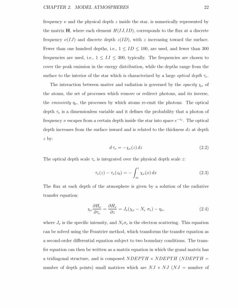
CHAPTER 2. MODEL ATMOSPHERES 22
frequency ν and the physical depth z inside the star, is numerically represented by
the matrix H, where each element H(IJ, ID), corresponds to the flux at a discrete
frequency ν(IJ) and discrete depth z(ID), with z increasing toward the surface.
Fewer than one hundred depths, i.e., 1 ≤ ID ≤ 100, are used, and fewer than 300
frequencies are used, i.e., 1 ≤ IJ ≤ 300, typically. The frequencies are chosen to
cover the peak emission in the energy distribution, while the depths range from the
surface to the interior of the star which is characterized by a large optical depth τν .
The interaction between matter and radiation is governed by the opacity χν of
the atoms, the set of processes which remove or redirect photons, and its inverse,
the emissivity ην , the processes by which atoms re-emit the photons. The optical
depth τν is a dimensionless variable and it defines the probability that a photon of
frequency ν escapes from a certain depth inside the star into space e−τν . The optical
depth increases from the surface inward and is related to the thickness dz at depth
z by:
d τν = −χν(z) dz (2.2)
The optical depth scale τν is integrated over the physical depth scale z:
τν(z) − τν(z0) = −∫ z
z0
χν(x) dx (2.3)
The flux at each depth of the atmosphere is given by a solution of the radiative
transfer equation:
χν∂Hν
∂τν
=∂Hν
∂z= Jν(χν − Ne σe) − ην , (2.4)
where Jν is the specific intensity, and Neσe is the electron scattering. This equation
can be solved using the Feautrier method, which transforms the transfer equation as
a second-order differential equation subject to two boundary conditions. The trans-
fer equation can then be written as a matrix equation in which the grand matrix has
a tridiagonal structure, and is composed NDEPTH × NDEPTH (NDEPTH =
number of depth points) small matrices which are NJ × NJ (NJ = number of

CHAPTER 2. MODEL ATMOSPHERES 23
frequency points). Details of this technique and others which are used to solve the
radiative transfer equation are given in Mihalas (1978). In the following section,
I will discuss how we accounted for convective energy transport, and, next, I will
discuss improvements to opacity calculations (χν).
2.2 Convective Transfer
The importance of convective energy transfer in cool stars has been recognized
for many years with the establishment of the Schwarzschild stability criterion and
the mixing-length theory for convective transfer. In particular, the modelling of
hydrogen-rich white dwarfs with temperatures below 14000 K requires convection
as one the forms of energy transfer (for helium-rich white dwarfs this temperature
is much higher). The importance of convective energy transfer in cool white dwarfs
was first recognized by Schatzman (1958), and the first attempt at calculating model
atmospheres with convection was done by Bohm (1968). The effect of convection
in white dwarfs was further investigated by Wickramasinghe & Strittmatter (1970),
who calculated model atmospheres for DA and DB white dwarf for temperatures
where convection produces significant changes in atmospheric structure. Van Horn
(1970) and Koester (1979) also calculated model atmospheres which included con-
vective energy transfer, but they also investigated the effect of convection on the
cooling of a white dwarf. Bues (1970) calculated models for helium rich white dwarfs
with a temperature range of 11,000 K to 21,000 K. Model atmospheres for cool hy-
drogen rich white dwarfs (7000 ≤ Teff ≤ 12000 K) were calculated and published
by Wehrse (1976), however he does not combine convective and radiative transfer
in the same models. Fontaine et al. (1974) investigated the effects of varying the
composition, equation of state, and the convective mixing length on the white dwarf
convection zones. The computation of model atmospheres became common, and
convection was included so that cool white dwarfs could be studied e.g. Shipman
CHAPTER 2. MODEL ATMOSPHERES 24
(1977), Koester (1979) and more recently Bergeron (1991; 1992b). Detailed dis-
cussions of the physical principles can be found in Clayton (1983), Mihalas (1978),
and Cox and Giuli (1968). In the following section, the theory of convective energy
transfer will be developed in detail, so that important variable numerical factors can
be identified as free parameters of the convection theory.
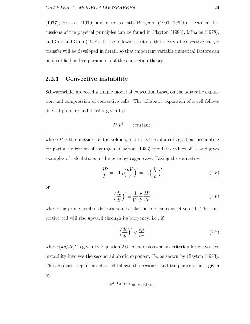
2.2.1 Convective instability
Schwarzschild proposed a simple model of convection based on the adiabatic expan-
sion and compression of convective cells. The adiabatic expansion of a cell follows
lines of pressure and density given by:
P V Γ1 = constant,
where P is the pressure, V the volume, and Γ1 is the adiabatic gradient accounting
for partial ionization of hydrogen. Clayton (1983) tabulates values of Γ1 and gives
examples of calculations in the pure hydrogen case. Taking the derivative:
dP
P= −Γ1
(dV
V
)′= Γ1
(dρ
ρ
)′, (2.5)
or (dρ
dr
)′=
1
Γ1
ρ
P
dP
dr, (2.6)
where the prime symbol denotes values taken inside the convective cell. The con-
vective cell will rise upward through its buoyancy, i.e., if:
(dρ
dr
)′<
dρ
dr, (2.7)
where (dρ/dr)′ is given by Equation 2.6. A more convenient criterion for convective
instability involves the second adiabatic exponent, Γ2, as shown by Clayton (1983).
The adiabatic expansion of a cell follows the pressure and temperature lines given
by:
P 1−Γ2 T Γ2 = constant.

CHAPTER 2. MODEL ATMOSPHERES 25
Taking the derivative:
dP
P= − Γ2
1 − Γ2
(dT
T
)′, (2.8)
or
−(dT
dr
)′= −Γ2 − 1
Γ2
T
P
dP
dr, (2.9)
where, again, the prime symbol denotes values taken inside the convective cell. In
pressure equilibrium, a decreasing density in the cell relative to the surroundings
must be accompanied by a temperature increase. Therefore, the instability criterion
for temperature derivations is mirrored on the density equation (Equation 2.7):
−(dT
dr
)′< −dT
dr, (2.10)
where (dT/dr)′ is given by Equation 2.9. If the temperature of the surroundings
decreases more steeply than the temperature inside the cell, then convection sets
in. Finally, we have assumed that the conditions inside the cell were adiabatic, it is
therefore appropriate to write the Schwarzschild instability criterion as:
−(dT
dr
)A
< −dT
dr, (2.11)
where
−(dT
dr
)A
= −Γ2 − 1
Γ2
T
P
dP
dr, (2.12)
2.2.2 Mixing length theory
The basic picture is familiar and involves the transport of a certain quantity of heat
in a convective cell. The net flux so transported depends on the density ρ of the
cell, the specific heat at constant pressure CP , the average speed upward of the cell
v, and the temperature difference between the cell and its surroundings ∆T . The
flux using the convention of Eddington is given by:
4πHconvective = ρ CP v ∆T (2.13)

CHAPTER 2. MODEL ATMOSPHERES 26
Temperature differential ∆T
The calculation of the temperature differential is central to the problem of convective
energy transport. The following definitions apply. The actual temperature gradient
in the atmosphere is:
∇ =d lnT
dr
/d lnP
dr=
d lnT
d lnP, (2.14)
and the temperature gradient in the convective cell is:
∇′ =(d ln T
dr
)′/d lnP
dr=(d lnT
d lnP
)′, (2.15)
where P is the total gas pressure and r is the radial distance. The adiabatic tem-
perature gradient defined in Equation 2.12 and written with the above convention
is:
∇A =Γ2 − 1
Γ2
(2.16)
The temperature difference between the convective cell and its surroundings is then
a function of the temperature gradient experienced by the cell as it moves upward
relative to the temperature gradient of the surroundings over a distance ∆r:
∆T = −∆r(dT
dr−(dT
dr
)′), (2.17)
where applying the trapezoidal rule ∆r = /2, and is the free-parameter of the
mixing-length theory. The mixing-length is an arbitrary factor of the pressure
scale-height h where
h−1 = −d ln P
dr=( P
ρg
)−1
(2.18)
where g is the local acceleration and assuming hydrostatic equilibrium. Therefore,
∆r =1
2
(
h
)h = −1
2
(
h
) (d ln P
dr
)−1
. (2.19)
Combining Equations 2.17 and 2.19 we have
∆T =1
2
(
h
) (d lnP
dr
)−1 (dT
dr−(dT
dr
)′)

CHAPTER 2. MODEL ATMOSPHERES 27
And using Equations 2.14 and 2.15 we have
∆T =1
2
(
h
)T (∇−∇′) (2.20)
Our new expression for the convective flux which combines Equations 2.13 and the
previous expression for ∆T is:
4πHconvective =1
2ρ CP v
(
h
)T (∇−∇′) (2.21)
Mean velocity of the convective cell, v
We now attempt to determine the average velocity v of the convective cell. Assuming
pressure equilibrium across the walls of the cell (dP = 0), the cell moves upward
due to its buoyancy. The buoyant force applied on the cell is:
fb = −g∆ρ, (2.22)
and ρ = µP/T , where µ is the mean molecular weight. Now, µ is a function of
P and T because the fraction of bound electrons is a function of temperature and
pressure. Therefore
d ln ρ = d lnµ+d lnP −d ln T =( ∂ ln µ
∂ ln T
)Pd lnT +
( ∂ ln µ
∂ ln P
)Td lnP +d lnP −d ln T
But we have already required that dP = 0, therefore:
d ln ρ = −(1 − ∂ ln µ
∂ ln T
)Pd lnT
∆ρ = −(1 − ∂ ln µ
∂ ln T
)Pρ∆T
T= −Qρ
∆T
T(2.23)
The quantity Q defined above is related to the adiabatic gradient ∇A by
Q =CP∇AρT
P(2.24)
Finally, using Equations 2.20 and 2.23, the buoyant force (Equation 2.22) is ex-
pressed in the terms of customary variables:
fb =1
2gQρ
(
h
)(∇−∇′) (2.25)

CHAPTER 2. MODEL ATMOSPHERES 28
We now estimate the work done on the cell: work =< force > · < distance >. The
average force is fb/2 and the average distance covered is /2, again following the
trapezoidal rule. therefore the average work is:
w =fb
2·
2=
1
8gQρ h
(
h
)2
(∇−∇′) (2.26)
Considering that half of the work will be lost to friction, the average velocity of the
cell is ρ v2/2 = w/2:
v =√
w/ρ =
√gQh
8
(
h
)(∇−∇′)1/2 (2.27)
And finally, combining Equation 2.21 and our previous expression for v:
4πHconvective =1
2ρ CP T
√gQh
8
(
h
)2
(∇−∇′)3/2 (2.28)
Radiative loss of the cell during transit
To complete the theory we examine the effect of radiative loss due to the (mild)
temperature gradient existing between the cell and its surroundings. The additional
energy stored in a convective cell of volume V relative to its surroundings is
E = ρ CP V ∆T (2.29)
For simplicity, the radiative loss in the cell is treated as optically thin (τ << 1) or
as optically thick (τ >> 1). In optically thick media, the diffusion approximation
holds, and the frequency integrated flux is given by:
F = 4π1
3
dB
dτR=
4π
3
dB
dT
dT
χRdz(2.30)
where B is the frequency-integrated Planck function, τR is the Rosseland-averaged
depth scale, and χR is the Rosseland-averaged opacity. The derivative dT/dz is
approximated by ≈ ∆T/ where ∆T is the temperature difference between the cell
and its surroundings and is the mixing length. Therefore
F =4π
3
1
χR
(4σRT 3
π
)∆T
(2.31)

CHAPTER 2. MODEL ATMOSPHERES 29
Suppose next that the cell irradiates uniformly over a lifetime /v and across a total
surface A. The energy loss is:
∆E = A · F ·
v= A
4π
3
1
χR
(4σRT 3
π
)∆T
v= A
16
3σRT 3∆T
1
vχR, (2.32)
and the efficiency γ with which convective cells carry energy is the ratio of the stored
energy E to the energy radiated away ∆E, γ = E/∆E. Combining Equations 2.29
and 2.32 in the optically thick limit, the efficiency is:
γthick = ρ CP V ∆T( 3
16
vχR
AσRT 3∆T
)=
ρ CP v
16σRT 33χR
(V
A
), (2.33)
Assuming that the convective cell is spherical, the ratio V/A is simply /3. Therefore
γthick =ρ CP v
16σRT 3χR · =
τ
2
(ρ CP v
8σRT 3
), (2.34)
where the optical depth of the cell is τ = χR · .
In optically thin media, the flux at the surface of a spherical cell is given by:
F = 4π(1
3
)∆B τ
2=
2
3π ∆B τ, (2.35)
where (1/3) is a geometrical factor, τ has the same meaning as before, and ∆B =
(dB/dT )∆T . Therefore, the total energy radiated by the convective cell during
transit time of /v is:
∆E = A · F ·
v= A · 2
3π(4σRT 3
π
)∆Tτ
v(2.36)
The efficiency is then
γthin = ρ CP V ∆T( 3
8AσRT 3∆Tτ
v
)=
1
τ
ρ CP v
8σRT 3
3V
A , (2.37)
And, as before, the ratio V/A of a sphere is /3. Finally
γthin =1
τ
(ρ CP v
8σRT 3
), (2.38)

CHAPTER 2. MODEL ATMOSPHERES 30
Equations 2.34 and 2.38 represent the limits of the general case given by the sum of
the two equations:
γ = γthin + γthick =ρ CP v
8σRT 3
(1
τ+
τ
2
)=
ρ CP v
8σRT 3
(1 + τ 2/2
τ
)(2.39)
The efficiency parameter γ can also be written in terms of gradients defined
previously. The additional energy carried by the cell is proportional to ∇ − ∇′
(see Equation 2.28) while the energy lost by radiation is the difference between the
maximum quantity of energy carried under adiabatic conditions ∇−∇A minus the
actual energy carried ∇−∇′. Therefore, the efficiency parameter can also be written
as
γ =∇−∇′
(∇−∇A) − (∇−∇′)=
∇−∇′
∇′ −∇A(2.40)
Combining the two expressions for γ and substituting v from Equation 2.27, we
have:
∇−∇′
∇′ −∇A=
ρ CP
8σRT 3
√gQh
8
(
h
)(∇−∇′)1/2
(1 + τ 2/2
τ
)(2.41)
It is customary to define the quantity B (unrelated to the Planck function) as:
B ≡ ∇′ −∇A
(∇−∇′)1/2=
8σRT 3
ρ CP
√8
gQh
(h
)( τ
1 + τ 2/2
), (2.42)
and to re-write the equation in terms of the unknown x = (∇−∇′)1/2:
Bx = (∇′−∇A)−(∇−∇A)+(∇−∇A) = −(∇′−∇)+(∇−∇A) = −x2 +(∇−∇A),
(2.43)
or
x2 + Bx − (∇−∇A) = 0. (2.44)
And then we solve this quadratic equation for x:
x = (∇−∇′)1/2 = −B
2+(B2
4+ (∇−∇A)
)1/2
(2.45)
The value for x = (∇−∇′)1/2 is then inserted in Equation 2.28:
4πHconvective =1
2ρ CP T
√gQh
8
(
h
)2
(∇−∇′)3/2 (2.46)
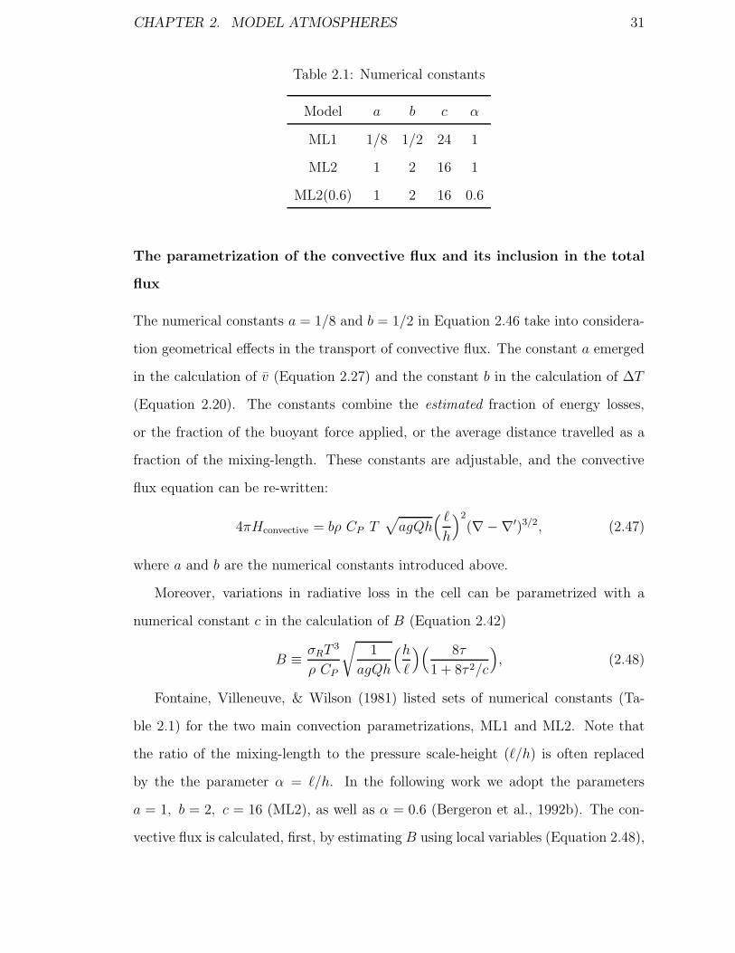
CHAPTER 2. MODEL ATMOSPHERES 31
Table 2.1: Numerical constants
Model a b c α
ML1 1/8 1/2 24 1
ML2 1 2 16 1
ML2(0.6) 1 2 16 0.6
The parametrization of the convective flux and its inclusion in the total
flux
The numerical constants a = 1/8 and b = 1/2 in Equation 2.46 take into considera-
tion geometrical effects in the transport of convective flux. The constant a emerged
in the calculation of v (Equation 2.27) and the constant b in the calculation of ∆T
(Equation 2.20). The constants combine the estimated fraction of energy losses,
or the fraction of the buoyant force applied, or the average distance travelled as a
fraction of the mixing-length. These constants are adjustable, and the convective
flux equation can be re-written:
4πHconvective = bρ CP T√
agQh(
h
)2
(∇−∇′)3/2, (2.47)
where a and b are the numerical constants introduced above.
Moreover, variations in radiative loss in the cell can be parametrized with a
numerical constant c in the calculation of B (Equation 2.42)
B ≡ σRT 3
ρ CP
√1
agQh
(h
)( 8τ
1 + 8τ 2/c
), (2.48)
Fontaine, Villeneuve, & Wilson (1981) listed sets of numerical constants (Ta-
ble 2.1) for the two main convection parametrizations, ML1 and ML2. Note that
the ratio of the mixing-length to the pressure scale-height ( /h) is often replaced
by the the parameter α = /h. In the following work we adopt the parameters
a = 1, b = 2, c = 16 (ML2), as well as α = 0.6 (Bergeron et al., 1992b). The con-
vective flux is calculated, first, by estimating B using local variables (Equation 2.48),
CHAPTER 2. MODEL ATMOSPHERES 32
then calculate (∇ − ∇′)1/2 (Equation 2.45), and, finally calculate Hconvective using
Equation 2.47 with the appropriate numerical constants.
Expressing the energy output with the frequency-integrated Eddington flux, the
equation for the conservation of energy, or radiative-convective equilibrium, is:
4πHtotal = 4πHconvective + 4π
∫ ∞
0
Hνdν = σRT 4eff , (2.49)
in replacement of Equation 2.1.
Figure 2.1 shows the fraction of energy that is transported by convection as a
function of the optical depth for models calculated for Teff = 7000 to 14000 K (in
steps of 1000 K) and log g = 7.0 to 9.5 (in steps of 0.5 dex). The figure shows
that the atmosphere is almost fully convective at greater optical depths for models
calculated at lower temperatures. At 14000 K convective energy transfer appear to
be negligible at low surface gravities, however at log g = 9.5, over 90% of energy is
still transported using convection at greater optical depths. Figure 2.2 also shows the
fraction of energy transported by convection, but for models calculated for Teff =
4500 to 6500 K (in steps of 500 K) and log g = 7.0, 8.0 and 9.0. At these low
temperatures almost all the energy is transported using convection.
Figure 2.3 shows the temperature as a function of the optical depth for Teff = 7000
to 14000 K (in steps of 1000 K) and log g = 7.0 to 9.5 (in steps of 0.5 dex). The figure
shows that the temperature gradient increases at optical depths greater than τR ∼0.1. When convection is introduced, the temperature gradient becomes shallower.
Figure 2.4 also shows the temperature structure, but for models calculated for Teff =
4500 to 6500 K (in steps of 500 K) and log g = 7.0, 8.0 and 9.0.
Figure 2.5 shows the total gas pressure as a function of the optical depth for
Teff = 7000 to 14000 K (in steps of 1000 K) and log g = 7.0 to 9.5 (in steps of
0.5 dex). As in the figures showing the temperature structure of the models, the
pressure gradient changes at the optical depth τR ∼ 0.1. Figure 2.6 also shows the
pressure structure, but for models calculated for Teff = 4500 to 6500 K (in steps of
500 K) and log g = 7.0, 8.0 and 9.0. Note that the pressure is higher for models

CHAPTER 2. MODEL ATMOSPHERES 33
with a lower effective temperature.
In the outermost layers of the atmosphere (τR � 0.1) the density is relatively
small favouring the formation of neutral hydrogen. Since hydrogen is mostly neutral,
the opacity is small, and most of the energy can be carried radiatively and the
temperature gradient remains very small. The total gas pressure gradient remains
relatively constant at these depths since it depends mostly on the particle density. At
larger optical depths (τR � 0.1) the density becomes large enough so that hydrogen
begins to be ionized, which causes an increase in the opacity. At larger opacities
the temperature gradient must increase to drive the flux through the atmosphere,
and once the temperature gradient becomes steeper than the adiabatic gradient,
then convection begins to transport some of the flux. Convection will lower the
temperature gradient and will reduce the pressure increase at deeper optical depths.
Finally, since convective energy transfer is efficient at higher densities, then energy in
atmospheres of stars with a higher surface gravity is more likely to be carried using
convection. For example compare the models calculated at log g = 9.5 where a large
amount of energy is transported using convection in atmospheres with log g = 9.5,
and at log g = 7.0 all the energy is transported radiatively.
2.3 Opacities
We assume that the atmosphere of the white dwarf is dominated by hydrogen. The
following absorption processes will determine the total opacity of the hydrogen gas
and must be taken into account in solving the radiative transfer equation (Equa-
tion 2.4):
- absorption by neutral hydrogen between bound levels (bound-bound), between
a bound level and the continuum of free states (bound-free), and between two
free states (free-free),
- bound-free and free-free absorption by the negative hydrogen ion (H−),

CHAPTER 2. MODEL ATMOSPHERES 34
Figure 2.1: The set of plots show the fraction of energy transported by convec-
tion as a function of the optical depth for 7000 ≤ Teff ≤ 14000 K and log
g = 7.0, 7.5, 8.0, 8.5, 9.0 and 9.5. Teff = 14000 K is shown in blue and Teff = 7000K
is shown in red.

CHAPTER 2. MODEL ATMOSPHERES 35
- and scattering of light by neutral hydrogen (H I Rayleigh), and by e− (Thom-
son).
Hydrogen line transitions (bound-bound) occur between principal quantum num-
bers n = l (lower level) and n = u (upper level). Hydrogen energy levels are given
by El = 13.595eV/l2. Because of spontaneous decay, i.e., spontaneous emission of a
photon, the energy levels have finite lifetime, and, therefore, a finite energy width
Γnat = ∆El/h, the natural width expressed in frequency units. Other mechanisms
which contribute to widen the energy levels have measurable effects on line spec-
troscopy. Before discussing hydrogen opacities in general, I will present details of
hydrogen line broadening.
2.3.1 Hydrogen line broadening
In white dwarfs, pressure broadening dominates over thermal broadening because
of the high density encountered in their atmospheres. Collisions, or interactions,
between particles and a perturbed atom induce changes in the energy levels of the
perturbed atoms, and corresponding changes in the electromagnetic frequency of
the atomic transitions
∆E
h= ∆ν =
Cn
Rn(2.50)
where R is the separation between the particles and the perturbed atom, n is the
power law index, and Cn is the interaction constant. Therefore, R−n describes the
type of potential the particles are subjected to during an interaction. Dipole-dipole
interactions are described by R−3 when the neutral particles are of the same species
(resonance interactions) and R−6 if the particles are of different species (Van der
Waals interactions). Interactions between atoms and charged particles are typed
linear Stark effect (R−2) for hydrogen atoms perturbed by protons or electrons, and
quadratic Stark effect (R−4) for most atoms perturbed by electrons.
Stark broadening is the result of perturbations by charged particles (protons
and electrons). Linear Stark broadening affects the Hydrogen lines and becomes

CHAPTER 2. MODEL ATMOSPHERES 36
dominant in white dwarfs with Teff � 10000 K since hydrogen is mostly ionized at
these temperatures.
We use the Stark line broadening tables calculated by T. Schoning and K. Butler
for Lyman (l = 1, u = 2, 3, 4, 5) and Balmer lines (l = 2, u = 3, 4, ..., 10). The line
profiles S are normalized to the full oscillator strength and the Stark profiles were
convolved with a normalized thermal Doppler profile characterized by a width ∆νD.
D =1
π1/2∆νDe−∆2ν/∆2νD (2.51)
where
∆νD =ν
c
√2kT
m(2.52)
For lower temperature, where hydrogen is mostly neutral, resonance broadening
and van der Waals broadening become dominant. For pure hydrogen atmospheres
resonance broadening is more dominant than van der Waals broadening (see Berg-
eron, Wesemael & Fontaine (1991)), therefore only resonance broadening will be
discussed and added to the code.
Resonance or self broadening occurs as a result of interaction of the radiation
atom with the surrounding neutral atoms. Resonance broadening was calculated
using the equations of Ali & Griem (1965; 1966) where the resonance damping
width of an atomic level n = u is given by:
γ3,u = 2(1 − 1/24)4π
√g1
guNn=1(H) C3,u = 24.086
√g1
guNn=1(H) C3,u (2.53)
where gu is the statistical weight of the level considered, Nn=1(H) is the population
of the ground level of hydrogen, and C3,u is the interaction constant:
C3,u =e2f1u
4πmeν1u= 2.015 × 10⁷f1u
ν1u. (2.54)
Here f1u and ν1u are the oscillator strength and the frequency for the transition
from ground state to level n = u. Cayrel and Traving (1960) state1 that the total
1”Berucksichtigt man nur die Verbreiterung des Terms n = 2, so wird der Absorptionskoeffizient

CHAPTER 2. MODEL ATMOSPHERES 37
resonance damping width of a transition from the lower level n = l to the upper
level n = u is the sum of γ3,l and γ3,u, i.e.
γ3 = γ3,l + γ3,u (2.55)
The normalized resonance profile R is given by a Lorentzian (damping) profile:
Rν =1
π
γ3/4π
(ν − ν0)2 + (γ/4π)2(2.56)
where ∫ ∞
0
Rν dν = 1 (2.57)
and consequently the integrated line strength is, as required, given by (πe2/mc)flu.
2.3.2 Total line absorption profile
The combined Stark (S) and resonance (Equation 2.56) profile is given by the con-
volution of the two normalized functions S and R, and the total line absorption
coefficient (”bound-bound”) of the i → j transition is given by:
αbbν,lu =
πe2
mcflu S ∗ R =
πe2
mcflu
∫ ∞
0
S(ν ′)R(ν − ν ′)dν ′ (2.58)
Because the Stark and resonance broadening mechanisms operate in different tem-
perature regime, one often dominates the other, and we approximated the convolu-
tion by a simple addition:
im Flugel einer durch Eigendruck verbreiterten Balmerlinie (If one considers only the widening of
the term n=2, then the absorption coefficient in the wing becomes one by self-pressure widened
Balmer lines)
χE =13π
e4
m2c4
λ12λ4f12f
∆λ2N0. (5)
Wir versuchen nun, auch die Verbreiterung des oberen Termes genahert zu berucksichtigen, indem
wir in (5) f12λ12 durch f12λ12 + f1nλ1n ersetzen, d.h. die Halbwertsbreiten der Terme einfach
addieren. (We try now to consider also the widening of the upper term approached by replacing
in (5) f12λ12 by f12λ12 + f1nλ1n, i.e. the half widths of the terms simply add.)”
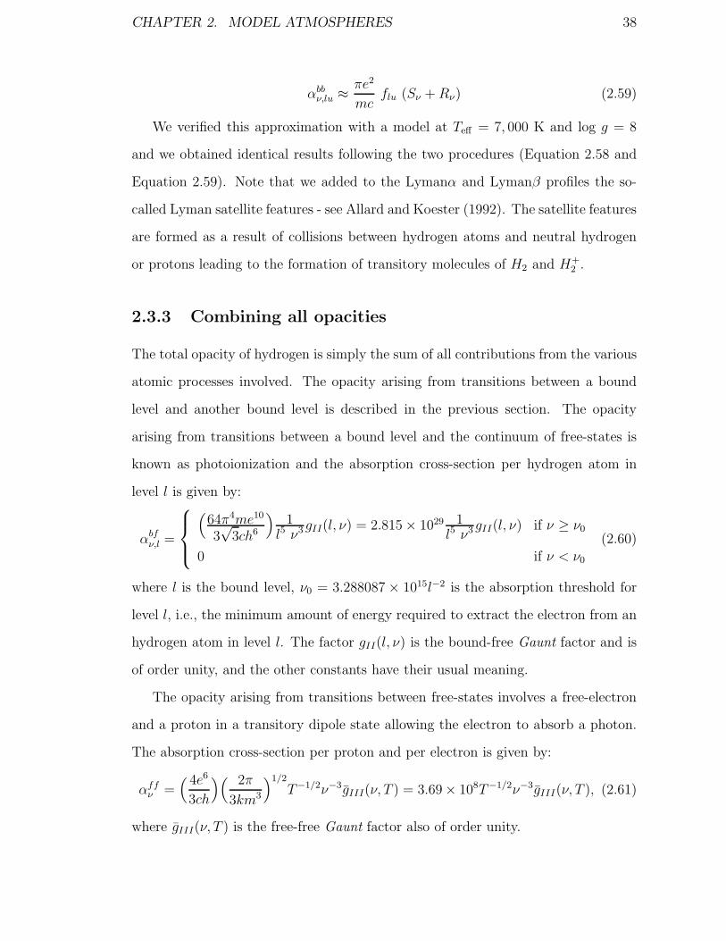
CHAPTER 2. MODEL ATMOSPHERES 38
αbbν,lu ≈ πe2
mcflu (Sν + Rν) (2.59)
We verified this approximation with a model at Teff = 7, 000 K and log g = 8
and we obtained identical results following the two procedures (Equation 2.58 and
Equation 2.59). Note that we added to the Lymanα and Lymanβ profiles the so-
called Lyman satellite features - see Allard and Koester (1992). The satellite features
are formed as a result of collisions between hydrogen atoms and neutral hydrogen
or protons leading to the formation of transitory molecules of H2 and H+2 .
2.3.3 Combining all opacities
The total opacity of hydrogen is simply the sum of all contributions from the various
atomic processes involved. The opacity arising from transitions between a bound
level and another bound level is described in the previous section. The opacity
arising from transitions between a bound level and the continuum of free-states is
known as photoionization and the absorption cross-section per hydrogen atom in
level l is given by:
αbfν,l =
(
64π4me10
3√
3ch6
)1
l5 ν3 gII(l, ν) = 2.815 × 1029 1l5 ν3 gII(l, ν) if ν ≥ ν0
0 if ν < ν0
(2.60)
where l is the bound level, ν0 = 3.288087 × 10¹⁵l−2 is the absorption threshold for
level l, i.e., the minimum amount of energy required to extract the electron from an
hydrogen atom in level l. The factor gII(l, ν) is the bound-free Gaunt factor and is
of order unity, and the other constants have their usual meaning.
The opacity arising from transitions between free-states involves a free-electron
and a proton in a transitory dipole state allowing the electron to absorb a photon.
The absorption cross-section per proton and per electron is given by:
αffν =
( 4e6
3ch
)( 2π
3km3
)1/2
T−1/2ν−3gIII(ν, T ) = 3.69× 10⁸T−1/2ν−3gIII(ν, T ), (2.61)
where gIII(ν, T ) is the free-free Gaunt factor also of order unity.

CHAPTER 2. MODEL ATMOSPHERES 39
In cooler layers one should expect the formation of the H− ion. We adopted
polynomial fits to the bound-free αbfν,H− and free-free αff
ν,H− cross-sections given by
Gray (1992).
The scattering of light by free electrons is known as Thomson scattering and the
cross-section per electron if given by
σe =8πe4
3m2c4= 6.65 × 10⁻²⁵ (2.62)
The Thomson cross-section is independent of frequency. The scattering of light by
neutral hydrogen, or Rayleigh scattering, is frequency dependent and is given by the
polynomial fit:
σRayleigh =
(0.5234
(νν0
)4
+ 1.219(
νν0
)6
+ 2.268(
νν0
)8)
× 10−24 if ν ≤ ν0
4.01 × 10⁻²⁴ if ν > ν0
(2.63)
where ν0 = 2.922 × 10¹⁵.
Finally, the total opacity of the hydrogen gas is given by:
χν =(∑
l
Nlαbfν,l+NeNpα
ffν +
∑l
Nl
∑u>l
αbbν,lu+NH−(αff
ν,H−+αbfν,H−)
)(1−e−hν/kT
)
+ Neσe + Nl=1σRayleigh (2.64)
where Nl and Nu are the populations of hydrogen (number of atoms per cm3 of gas)
in states l and u, respectively, Np is the proton population, and Ne is the number
of electrons per cm3 of gas.
2.4 Synthetic spectra
Having calculated the temperature and density structure of a white dwarf of sur-
face gravity log g and effective temperature Teff , a solution of the radiative transfer
equation provides Hν(z = 0) the surface Eddington flux. These synthetic spectra
are used for comparison with observed stellar spectra and for a determination of

CHAPTER 2. MODEL ATMOSPHERES 40
the stellar surface gravity log g∗ and effective temperature Teff,∗. Figures 2.7 and 2.8
show synthetic spectra for effective temperatures ranging from 5000 to 84000 K at
a surface gravity of log g = 8.0. The spectra show how the Balmer line profiles vary
with temperature.
Figure 2.9 shows details of the Balmer line profiles for varying log g and Teff .
The effect of including resonance broadening is shown by comparing spectral line
profiles which include resonance broadening to line profiles which do not. Resonance
broadening becomes prominent in the lower temperature models (i.e., Teff ≤ 8000)
where neutral hydrogen atoms are more numerous and hence are more likely to
interact with the emitting atoms.
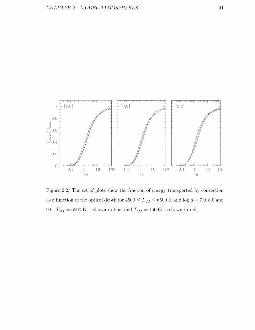
CHAPTER 2. MODEL ATMOSPHERES 41
Figure 2.2: The set of plots show the fraction of energy transported by convection
as a function of the optical depth for 4500 ≤ Teff ≤ 6500 K and log g = 7.0, 8.0 and
9.0. Teff = 6500 K is shown in blue and Teff = 4500K is shown in red.

CHAPTER 2. MODEL ATMOSPHERES 42
Figure 2.3: The temperature as a function of optical depth is shown for models at
7000 ≤ Teff ≤ 14000 K and log g = 7.0, 7.5, 8.0, 8.5, 9.0 and 9.5. Teff = 14000 K is
shown in blue and and Teff = 7000K is shown in red.
CHAPTER 2. MODEL ATMOSPHERES 43
Figure 2.4: The temperature as a function of optical depth is shown for models at
4500 ≤ Teff ≤ 6500 K and log g = 7.0, 8.0 and 9.0. Teff = 6500 K is shown in blue
and and Teff = 4500K is shown in red.

CHAPTER 2. MODEL ATMOSPHERES 44
Figure 2.5: The total gas pressure as a function of optical depth is shown for models
at 7000 ≤ Teff ≤ 14000 K and log g = 7.0, 7.5, 8.0, 8.5, 9.0 and 9.5. Teff = 14000 K
is shown in blue and and Teff = 7000K is shown in red.

CHAPTER 2. MODEL ATMOSPHERES 45
Figure 2.6: The total gas pressure as a function of depth is shown for models at
4500 ≤ Teff ≤ 6500 K and log g = 7.0, 8.0 and 9.0. Teff = 6500 K is shown in blue
and and Teff = 4500K is shown in red.

CHAPTER 2. MODEL ATMOSPHERES 46
Figure 2.7: Synthetic spectra showing Balmer lines at log g = 8 for Teff = 5000 K to
14000 K at intervals of 1000 K.

CHAPTER 2. MODEL ATMOSPHERES 47
Figure 2.8: Synthetic spectra showing Balmer lines at log g = 8 for Teff = 16000 K
to 84000 K at intervals of 4000 K.

CHAPTER 2. MODEL ATMOSPHERES 48
Figure 2.9: The line profiles of Hα to Hε are shown (from bottom to top) for the
given temperature and surface gravity. The profiles shown in red include resonance
broadening and the profiles in black do not.
Chapter 3
Properties of Local White Dwarfs:
Temperature, Gravity and
Magnetic Fields
3.1 Introduction
The study of white dwarfs in the local neighbourhood can contribute toward our
understanding of the formation and evolution of stars in the Galactic plane. In
this chapter, the first two questions (see page 6) will be dealt with. That is, the
distribution and origin of magnetic fields in white dwarfs will be investigated, and
the white dwarfs in the Solar neighbourhood will be revisited, including a search for
new white dwarf stars using the revised NLTT catalog (Salim and Gould, 2003).
Numerous surveys have searched for magnetic fields in white dwarfs. Most of
these surveys used circular polarization as a method of finding new magnetic white
dwarfs. Angel, Borra & Landstreet (1981) observed 13 magnetic white dwarfs,
where five of these were new discoveries, in their survey of over 100 white dwarfs.
A more recent survey was conducted by Schmidt & Smith (1995), who searched
for low-field magnetic white dwarfs. They observed 169 DA white dwarfs with a
49
CHAPTER 3. PROPERTIES OF LOCAL WHITE DWARFS 50
temperature subclass θ = 50400/T = 2 to 8, an apparent magnitude mB ≤ 15.0,
and a declination δ ≥ −30◦. They found 4 of them to be magnetic with B� ∼ 30−330
kG. Putney (1997) conducted a survey of 52 DC white dwarfs with V ≤ 16.5 and
δ ≥ −20◦, and detected 4 new magnetic stars (one with B� ∼ 40 kG and three with
B� ∼ 5 − 220 MG). Fabrika & Valyavin (1999) observed 16 DA white dwarfs, with
12 of them overlapping with Schmidt & Smith (1995). They also observed 40 Eri
B, and measured a variable magnetic field with an amplitude of B� ∼ 2.5 kG.
All these surveys have included stars that are found mainly in the northern
hemisphere, which means that the southern stars have not been studied to the same
extent. Therefore, a spectropolarimetric survey of white dwarfs in the southern
hemisphere was conducted as part of this thesis. For this survey, 65 white dwarfs
with V � 16.4 and δ � −30◦ have been observed, with 55 of these having V � 15.
Five of the brighter candidates were in close binaries (1 double degenerate and 4 DA
+ dMe). The candidate list also included four white dwarfs which were re-classified
as subdwarf B (sdB) stars as a result of this survey. The magnetic white dwarf
EUVE J0823−254 was included in the survey as a case study.
Holberg, Oswalt & Sion (2002) found the local space density of white dwarfs
to be 5.0 ± 0.7 × 10⁻³ pc−3 based on the known white dwarfs found within 20 pc
of the Sun. They found that the local sample is only complete to 13 pc, and that
up to 20 pc approximately 50 white dwarfs still remain to be discovered. Many
stars in Luyten’s NLTT catalogue (Luyten, 1979) remain unclassified, and there
is a potential for new nearby white dwarfs to be discovered, therefore as part of
this thesis some white dwarf candidates that have been chosen on the basis of their
proper motion and their optical/infrared colours have been observed.
In this chapter, I will first explain the necessary background information required
for the analysis of magnetic fields from spectroscopy and spectropolarimetry. The
observations will be presented in section 3.3 and the data reduction and analysis of
the spectropolarimetric survey of southern white dwarfs will be presented in section
CHAPTER 3. PROPERTIES OF LOCAL WHITE DWARFS 51
3.4. This section will also present the results of the survey. The origin of magnetic
fields in white dwarfs will be discussed in section 3.5, in particular the assumption
that magnetic Ap and Bp stars are the progenitors of magnetic white dwarfs will
be tested. In section 3.6, I will revisit the local population of white dwarfs and
discuss the incidence of magnetism among white dwarfs, obtain atmospheric param-
eters for a selected number of them, and present new spectroscopically identified
white dwarfs. White dwarf candidates from the revised NLTT catalog will also be
presented, including a kinematical study of these objects. Finally, I will discuss the
results of the work on local white dwarfs in section 3.6.3, and summarize in section
3.7.
3.2 Techniques for Measuring Magnetic Fields
3.2.1 Zeeman Spectroscopy
Since most white dwarfs observed in spectropolarimetric surveys are hydrogen-rich
(spectral type DA), the Zeeman splitting effect will be explained with the hydrogen
atom as an example.
In the presence of an external magnetic field, a free electron can take different
energy levels according to:
EN = (N +1
2)�ωC, N = 0, 1, ... (3.1)
with
ωC =2π
λC=
eB
mec, (3.2)
being the electron cyclotron frequency, and λC being defined as the electron cy-
clotron wavelength. This applies to free electrons and the energy levels are equally
spaced.
For electrons in a bound state, such as the electron in a hydrogen atom, the

CHAPTER 3. PROPERTIES OF LOCAL WHITE DWARFS 52
energy levels are given by:
En = −�ωR
n2, (3.3)
where n is the principal quantum number and ωR is the Rydberg frequency. These
are the energy levels of an electron due to the electrostatic potential where each level
n has a n2 degeneracy. When the hydrogen atom is placed in a general magnetic
field, B, the energy levels can be given by the eigenvalues of the Hamiltonian, by
solving the Schrodinger equation. Since the relationship between B and the energy
levels are non-linear, an approximation of the relationship can be made for B > 104
G, this is where the spin and orbital angular momenta are effectively decoupled,
and this is known as the Paschen-Back effect. The Hamiltonian is (Garstang and
Kemic, 1974; Wickramasinghe and Ferrario, 2000):
H =p2
2me
− e2
r+
1
2ωC(lz + 2sz) +
1
8meω
2Cr2 sin2 θ, (3.4)
where r is the radial distance of the electron from the proton, with θ being the polar
angle measured with respect to the direction of the field, p is the linear momentum
and lz and sz are the operators for the orbital and spin angular momenta projected
along the field. The first term refers to the kinetic energy of the electron, the
second term to the Coulomb potential, the third to the interaction of the atom’s
magnetic moment with the applied magnetic field (the paramagnetic component),
and the final term refers to the coupling between the external field and the induced
magnetic effects (also known as the diamagnetic component).
For strong fields, the diamagnetic term dominates the paramagnetic term since it
depends on B2, and for weak fields (β = B/4.7×109G<< 1) the paramagnetic term
dominates and can be treated as a perturbation. The energy eigenvalues behave
linearly for small changes, therefore the energy level is shifted by the amount:
∆E =ml�ωC
2, (3.5)
where ml is the orbital magnetic quantum number with −l ≤ ml ≤ +l. This can

CHAPTER 3. PROPERTIES OF LOCAL WHITE DWARFS 53
be compared to the orbital electron where the shifts in the frequency are in units of
the Larmor frequency (ωL = ωC/2) and each level is split into 2n − 1 levels. The
transitions must obey the selection rule ∆ml = 0,±1, which means that it will be
split into three components. First, there is the unshifted π component for ∆ml = 0
and then the two σ shifted components for ∆ml = ±1. Therefore, the energy level
shift corresponds to the wavelength shift of:
∆λ = ± eλ2B
4πmec2≈ ±4.67 × 10⁻⁷λ2B, (3.6)
where λ is the wavelength in A and B is the magnetic field in MG. This approxima-
tion can be used for Balmer lines for fields up to ∼ 10 MG. For magnetic fields less
than ∼ 1 MG, the Zeeman splitting is difficult to observe in white dwarfs because
the spectral lines are broad in their high-density atmospheres. However, the Zeeman
splitting may be observed using spectropolarimetry to detect fields that are a few
tens of kG.
The Zeeman splitting observed represents the mean magnetic field across the
surface of the star, i.e., mean surface field. If the magnetic field is assumed to be
a dipole then the mean surface magnetic field can be related to the polar magnetic
field by:
Bs =Bp
2
√1 + 3 cos2 θ, (3.7)
where Bp is the polar field, and θ is the angle between the magnetic field and the
line of sight.
3.2.2 Spectropolarimetry
Spectropolarimetry as mentioned in the previous section is one of the techniques used
to detect magnetic fields. By measuring the circular polarization, the longitudinal
component of the magnetic field can be determined, which is at most 40% of the
dipole field (i.e. B� = 0.4Bd cos i; Schmidt & Smith (1995)). For magnetic fields

CHAPTER 3. PROPERTIES OF LOCAL WHITE DWARFS 54
where the Zeeman splitting cannot be observed, spectropolarimetry can be used to
detect the fields that are less than 1 MG.
The electron in an atom can be modelled as a linear harmonic oscillator with a
frequency ω0. If the atom is placed in a magnetic field then this oscillator will precess
about the magnetic field and will be equivalent to a linear oscillator of frequency
ω0 along the field. This describes the π component which will be linearly polarized.
The σ components will precess along the field as circular oscillators with frequencies,
ω0−ωL which would rotate about the magnetic field like a free electron and ω0 +ωL,
which would rotate about the magnetic field in the opposite direction.
The π component which acts as a linear oscillator will always be linearly polar-
ized, maximum linear polarization is observed when the magnetic field is perpendic-
ular to the line of sight and zero linear polarization is observed when the magnetic
field is aligned parallel to the line of sight. The σ components which act as circular
oscillators will be circularly polarized when the magnetic field is parallel to the line
of sight, linearly polarized when the magnetic field is perpendicular to the line of
sight and elliptically polarized for all other viewing direction. Therefore, by observ-
ing the flux in both circular and linear polarization, the geometry of the magnetic
field may be determined.
The polarization of spectral lines can be measured in terms of the Stokes param-
eters, where I, V , Q and U are the parameters (Mathys, 1989). I measures the total
intensity of the electromagnetic radiation, V is defined as the difference between the
right circularly polarized light and the left circularly polarized light and Q and U
measure linear polarization. The fraction of circular polarization in the spectrum is
defined by:
v =V
I=
I+ − I−I+ + I−
=∆I
2∆λ
2∆λ
I, (3.8)
where I+ and I− are the flux intensities of the right and left circularly polarized
radiation, respectively. The relative shift between the right and left circularly polar-
ized spectra is twice the Zeeman shift ∆λ (see Equation 3.6). For ∆λ much smaller

CHAPTER 3. PROPERTIES OF LOCAL WHITE DWARFS 55
than the line width:
∆I
2∆λ≈ dI−
dλ≈ dI+
dλ≈ 1
2
dI
dλ, (3.9)
and combining Equations 3.8 and 3.9:
v =1
2
dI
dλ
2 · 4.67 × 10−13λ2B�
I=
dI
dλ
4.67 × 10⁻¹³λ2B�
I, (3.10)
where B� is the mean longitudinal magnetic field in Gauss. Therefore, the longitu-
dinal field strength can be determined directly from the measured polarization (v)
and intensity (I) spectra. Equation 3.10 can only be used for weak magnetic fields
where the Zeeman splitting is smaller than the width of the line profile.
3.3 Observations
3.3.1 Spectropolarimetry
The data for the survey of magnetic fields in southern white dwarfs has been ac-
quired at the 74-inch telescope at the Mt. Stromlo Observatory using the Steward
Observatory CCD Spectropolarimeter. The instrument is described in Schmidt,
Stockman & Smith (1992b), however the instrument setup has been updated and
modified for the 74-inch telescope, with an improved camera lens and a thinned,
back illuminated LORAL 1200 × 800 CCD with near unity quantum efficiency and
< 6e− read noise. The f/18 Cassegrain telescope beam was adapted to the f/9
spectrograph optics with a small converging lens placed infront of the slit. A 964
lines mm−1 grating blazed at 4639 A was used which gave a dispersion of 2.62 A
per pixel. Circular polarized spectra of white dwarfs were obtained over a region
which includes Hα, Hβ and Hγ, with a spectral resolution of ∼ 9 A. The data were
acquired in multiple waveplate sequences. Table C.1 lists the objects observed using
the spectropolarimeter with UT dates and the number of exposures times the length
of each exposure. The length of an exposure is the time required for one waveplate
sequence to be completed. One waveplate sequence is a series of four exposures at

CHAPTER 3. PROPERTIES OF LOCAL WHITE DWARFS 56
different quarter-waveplate orientation which produces two complementary images
of opposite senses of circular polarization. The slit width was set at 2.4′′, however it
was increased to 3.6′′ when the seeing deteriorated. Flux and polarization spectra of
the observed objects are presented in Figure C.1. The observations for this survey
were carried out by Gary D. Schmidt, Stephane Vennes and myself.
3.3.2 Complementary Spectroscopy
Additional spectroscopy of many of the white dwarfs in the survey have been ob-
tained using the 74-inch telescope with the Cassegrain spectrograph equipped with
a 300 line mm−1 grating blazed at 5000 A and a 2k × 4k CCD binned 2 × 2. This
resulted in a wavelength dispersion of 2.85 A per pixel and a spectral range of about
3500 A to 6400 A. The observation log for these observations is given in Table C.2.
The complementary observations were carried out by Stephane Vennes and myself.
3.3.3 Spectroscopy of NLTT Stars
The observations of NLTT white dwarf candidates, and of the five stars for which
confirmation of their spectral type was required are given in Table D.1.
The observations at MSO were carried out using the 74inch telescope using the
300 line mm−1 grating blazed at 5000 A and the 2k × 4k CCD camera binned 2× 2
(and a 600 line mm−1 grating blazed at 5000 A). The spectra had a range of 3850 to
7500 A with a dispersion of 2.83 A pixel−1 and a spectral resolution of ≈ 8 A. FeAr
arc exposures of 120 seconds and FeNe arc exposures of 5 seconds were frequently
acquired and the spectra were calibrated with the flux standards EG 131, Feige 110,
and EG 21. To minimize atmospheric dispersion losses at short wavelengths the slit
was aligned along the parallactic angle for the December observing run.
The observations carried out at Siding Spring Observatory were obtained using
the Double-Beam Spectrograph attached to the 2.3 m telescope. The 300 line mm−1
grating blazed at 4200 A was used in the blue arm to obtain a spectral range of 3410

CHAPTER 3. PROPERTIES OF LOCAL WHITE DWARFS 57
to 6140 A with a dispersion of 2.18 A per pixel. The 316 line mm−1 grating blazed
at 7500 A was used in the red arm to obtain a spectral range of 5530 to 9120 A
with a dispersion of 2.08 A per pixel. A dichroic was used to split the beam of light
into two beams so that the red and blue spectra could be obtained simultaneously.
Two SITE 1752 × 532 CCD cameras were reduced to 1300 × 200 in the red and
1752 × 200 in the blue. Frequent CuAr arc exposures of 20 seconds and 1 second
were taken in the blue and red, respectively. The spectra were calibrated with the
flux standard EG 21 and EG 131. The slit was aligned along the parallactic angle
to avoid atmospheric dispersion losses at short wavelengths.
Three stars, NLTT 529, NLTT 19138 and NLTT 40607 were observed using the
modular spectrograph attached to the Hiltner 2.4 m telescope at MDM Observatory
on 2002 December 16, 2003 February 3, and June 22. These observations were
carried out by John R. Thorstensen. The SITE 2048 × 2048 CCD and the 600
line mm−1 grating was used to obtain a spectral range of 4210 to 7540 A with
substantial vignetting toward the ends of this range. The 1 arcsec slit width gave
a spectral resolution of ∼ 3.2 A. The main observing program required accurate
radial velocities, the procedures used gave stability better than 10 km s−1. The slit
was rotated to the parallactic angle when observing was carried out at substantial
airmasses. Flux standards were observed nearly every clear night, generally two per
twilight, and a calibration for each observing run was derived from these. Prior to
flux calibration all the data were divided by a mean hot-star continuum, in order to
remove the gross sensitivity variation and the resulting flux calibration was easily
fitted with a low-order polynomial. However, despite all these precautions, the
continua often show a ’wavy‘ distortion of an unknown origin. Repeat observations
of standards and hot stars show this to be present in the raw data, and not an
artifact of the calibration process. Therefore the continua in the MDM data must
be interpreted with caution.
All the spectra were reduced using the standard IRAF routines.

CHAPTER 3. PROPERTIES OF LOCAL WHITE DWARFS 58
3.4 Analysis
The code used to determine the magnetic field strength from the circular polarization
spectra was written by Gary Schmidt in Fortran 77 (referred to as GS from here on).
The code reads in the wavelength, circular polarization and the normalized flux. The
magnetic field for a specific absorption line is measured using Equation 3.10 where
the gradient (dF/dλ) is calculated at each wavelength bin from a pseudo-Lorentzian
fit to the line profile of the normalized flux. A pseudo-Lorentzian profile is used to
calculate the gradient to reduce the effects of noise. The magnetic field is derived
from the gradient of the line profile and the measured circular polarization at each
wavelength bin. The quoted B� is the weighted average of B� at each wavelength
bin in the line profile. The uncertainty of this value is taken from two sources, the
first is the uncertainty in the fit of the line profile (σprof) which is used to calculate
the gradient and the second is derived from the noise of the circular polarization
spectrum (σnoise). The major contribution to the uncertainty in B� is σnoise, where
the noise of the circular polarization spectrum is converted to an error of B� at
each wavelength using error propagation. Therefore the error in B� (i.e. σnoise) is
1/√
(∑
1/σi) where σi are the errors calculated at each wavelength bin. The total
uncertainty in B� is taken as√
σ2prof + σ2
noise.
The survey for magnetism yielded no detections of new magnetic white dwarfs,
however the survey will help constrain the fraction of magnetic white dwarfs in the
local neighbourhood.
Figure 3.1 shows the number distribution of measured magnetic field strengths
compared to a gaussian distribution with a standard deviation of 9.5 kG and the
number distribution of the measurements divided by its error (B�/∆B�). The mag-
netic field strength for each observation was taken as the weighted mean of mea-
surements for each of the Balmer lines. A plot of the measurement of the magnetic
field divided by the error should produce a standard gaussian distribution, however
the distribution has a standard deviation of 1.5. This could be a result of the code,

CHAPTER 3. PROPERTIES OF LOCAL WHITE DWARFS 59
Figure 3.1: Number distribution of measured magnetic field strengths (Ntotal = 86)
compared to a gaussian distribution with a standard deviation of 9.5 kG (left), and
the number distribution of the measurements divided by their error and compared
to a standard gaussian distribution (right).
CHAPTER 3. PROPERTIES OF LOCAL WHITE DWARFS 60
which may be calculating errors that are underestimated.
To test the error calculations in the code, a set of 250 synthetic spectra were
computed at a temperature of 16000 K and a surface gravity of log g = 8.0, with the
circular polarization set to zero at all wavelengths. Gaussian noise was added to both
the flux and circular polarization spectra. The simulated noise was assumed to have
a gaussian distribution because the noise of the observed spectra displayed a gaussian
distribution. The magnetic field was determined for these spectra using the GS code,
and was plotted as a number distribution of B�/∆B�. A weighted average of Hα, Hβ
and Hγ measurements was calculated. The distribution of B�/∆B� was compared
to a standard gaussian distribution using a Kolmogorov-Smirnov (KS) test. The
gaussian distribution was generated using the GASDEV function from Numerical
Recipes (Press et al., 1992). The top left panel of Figure 3.2 shows that the number
distribution of measured magnetic field strengths has a gaussian distribution with
a standard deviation of 4.0 kG. This standard deviation is entirely due to the noise
in the spectra. The centre left panel shows the number distribution of the magnetic
field measurements divided by its error. This distribution has a standard deviation
of σ = 1 showing that the calculated errors are not underestimated. And finally the
bottom left panel shows the cumulative distribution of the measurements divided
by its errors compared to a cumulative standard gaussian distribution. The KS test
shows that the distribution is a standard gaussian distribution with 95% certainty.
A second set of 250 synthetic spectra was computed which assumed a gaussian
distribution of magnetic fields with a mean of zero and a standard deviation of 6 kG.
The normalized flux spectrum was assumed to be the same as for the non-magnetic
white dwarfs since the broadening from the magnetic field will be negligible for the
broad white dwarf Balmer lines. The circular polarization spectra were calculated
using equation 3.10, and gaussian noise was added to both types of spectra. And,
like the previous set of measurements a weighted average of the Hα, Hβ and Hγ
measurements was calculated. Again, the distribution of the B�/∆B� measurements

CHAPTER 3. PROPERTIES OF LOCAL WHITE DWARFS 61
determined from this set of synthetic spectra was compared to a standard gaussian
distribution using a KS test. The top right panel of Figure 3.2 shows that the number
distribution of measured magnetic field strengths has a gaussian distribution with
a standard deviation of 10.0 kG, which is just the combination of the distribution
of magnetic fields and the errors of the measurement. The centre right panel shows
the number distribution of the magnetic field measurements divided by its error
compared to a standard gaussian distribution and a gaussian distribution with a
standard deviation of 1.8. And, finally the bottom right panel shows the cumulative
distribution of the measurements divided by its errors compared to a cumulative
standard gaussian distribution. The KS test shows that the probability that this
distribution is a standard gaussian distribution is much smaller than 1%. Therefore,
by introducing an external change, such as an underlying magnetic field distribution,
the B�/∆B� distribution is widened.
The KS-tests showed that the GS code calculates reliable uncertainties. There-
fore, any increase in the spread of the distribution of B/∆B is a result of either
an underlying low-field magnetic field distribution for white dwarfs or is a result of
external systematic errors which the GS code does not take into account since it only
calculates statistical errors. The presence of an underlying low magnetic field white
dwarf population is unlikely, since a ‘minisurvey’ by Schmidt & Smith (1995) of 7
bright white dwarfs, with measured uncertainties of 1 kG, resulted in no detection
of magnetism in any of these white dwarfs. Therefore, the errors were increased by
50% above their statistical values to account for systematic effects which are due
to a combination of factors. These factors include changing observation conditions
while the sequence of spectra taken at different waveplate positions was in progress.
Some of the observations were obtained during nights when the seeing was variable
or when high cirrus clouds were present, and the flux measured during the different
waveplate sequence exposures may vary.

CHAPTER 3. PROPERTIES OF LOCAL WHITE DWARFS 62
Figure 3.2: Comparison of magnetic field measurements of synthetic spectra which
assumed a zero field (left) and with an assumed magnetic field distribution which
has mean of zero and standard deviation of 6 kG (right). The top panels show the
number distributions of the measured magnetic fields for the two sets of synthetic
spectra, the centre panels show the number distribution of B�/∆B�, and finally the
bottom panels show the comparison of the cumulative distribution of B�/∆B� com-
pared to the cumulative standard gaussian distribution. The calculated KS proba-
bility that the observed distribution is the same as a standard gaussian distribution
is also given.

CHAPTER 3. PROPERTIES OF LOCAL WHITE DWARFS 63
3.4.1 Single White Dwarfs
Table 3.1 shows the white dwarfs observed with their apparent magnitude, measured
longitudinal fields, effective temperature, surface gravity and distance. References
are given for the effective temperature and surface gravity measurements. Where no
published effective temperature or surface gravity measurements are available, the
white dwarfs were formally compared to a grid of spectra. The grid of models extend
from Teff = 4500 to 6500 at (in steps of 500 K) at log g = 7.0, 8.0 and 9.0, and
Teff = 7000 to 16000 K (in steps of 1000 K) and 18000 to 32000 K (in steps of 2000
K) and 36000 to 84000 K (in steps of 4000 K) at log g = 7.0, 7.5, 8.0, 8.5, 9.0 and
9.5. The Balmer lines (Hα/Hβ to Hε/H8) were compared to model spectra using χ2
minimization techniques and the quoted uncertainties are statistical and do not take
into account possible systematic effects. For 50 of these stars, spectropolarimetry
was obtained.
Magnetic properties of five stars in the spectropolarimetric survey have been dis-
cussed in the literature, therefore these properties will be summarized and compared
to the results of this study.
LB 9802 This white dwarf is the visual companion to the high-field ultramas-
sive white dwarf, EUVE J0317−85.5. This study finds that the longitudinal field
measurement of LB 9802 is 7.16 ± 4.18 kG, which implies that this star is a non-
magnetic white dwarf. Figure 3.4 shows the flux and polarization spectra of LB
9802. The magnetic companion EUVE J0317−85.5 has been extensively observed
as part of another project during the period of the survey of white dwarf stars.
EUVE J0317−85.5 is an ultramassive white dwarf with a high magnetic field. The
star was found to vary over a 12 minute (725.4± 0.9 seconds) cycle (Barstow et al.,
1995a). A more accurate period of 725.7277 seconds was determined from the spec-
tropolarimetry during the survey and EUV E photometry (Vennes et al., 2003).
The additional observations of this white dwarf suggest that this star may have an
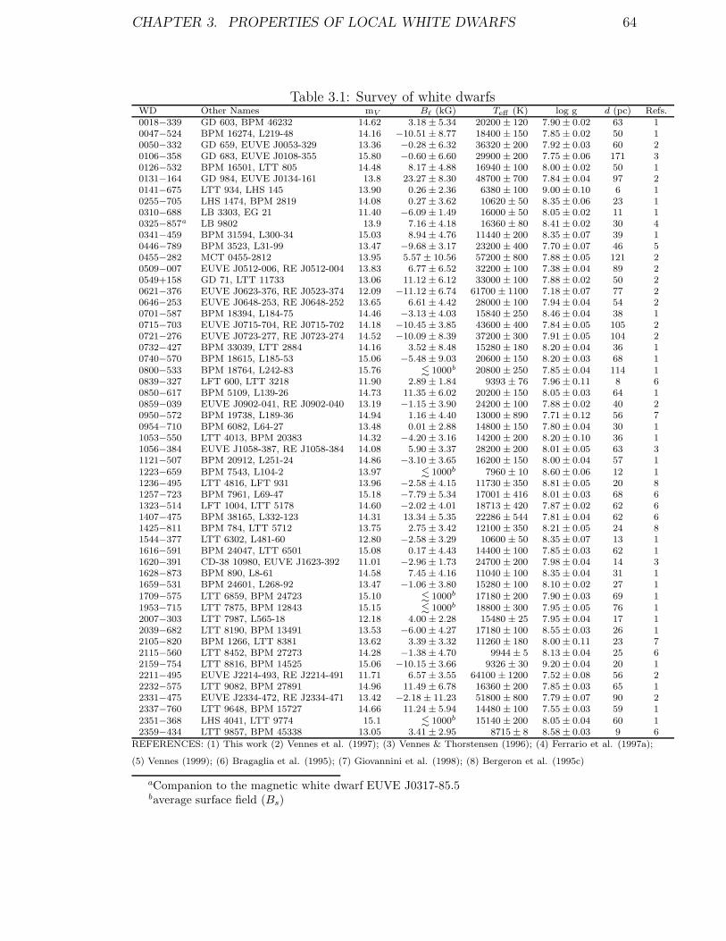
CHAPTER 3. PROPERTIES OF LOCAL WHITE DWARFS 64
Table 3.1: Survey of white dwarfsWD Other Names mV B� (kG) Teff (K) log g d (pc) Refs.0018−339 GD 603, BPM 46232 14.62 3.18 ± 5.34 20200 ± 120 7.90 ± 0.02 63 10047−524 BPM 16274, L219-48 14.16 −10.51 ± 8.77 18400 ± 150 7.85 ± 0.02 50 10050−332 GD 659, EUVE J0053-329 13.36 −0.28 ± 6.32 36320 ± 200 7.92 ± 0.03 60 20106−358 GD 683, EUVE J0108-355 15.80 −0.60 ± 6.60 29900 ± 200 7.75 ± 0.06 171 30126−532 BPM 16501, LTT 805 14.48 8.17 ± 4.88 16940 ± 100 8.00 ± 0.02 50 10131−164 GD 984, EUVE J0134-161 13.8 23.27 ± 8.30 48700 ± 700 7.84 ± 0.04 97 20141−675 LTT 934, LHS 145 13.90 0.26 ± 2.36 6380 ± 100 9.00 ± 0.10 6 10255−705 LHS 1474, BPM 2819 14.08 0.27 ± 3.62 10620 ± 50 8.35 ± 0.06 23 10310−688 LB 3303, EG 21 11.40 −6.09 ± 1.49 16000 ± 50 8.05 ± 0.02 11 10325−857a LB 9802 13.9 7.16 ± 4.18 16360 ± 80 8.41 ± 0.02 30 40341−459 BPM 31594, L300-34 15.03 8.94 ± 4.76 11440 ± 200 8.35 ± 0.07 39 10446−789 BPM 3523, L31-99 13.47 −9.68 ± 3.17 23200 ± 400 7.70 ± 0.07 46 50455−282 MCT 0455-2812 13.95 5.57 ± 10.56 57200 ± 800 7.88 ± 0.05 121 20509−007 EUVE J0512-006, RE J0512-004 13.83 6.77 ± 6.52 32200 ± 100 7.38 ± 0.04 89 20549+158 GD 71, LTT 11733 13.06 11.12 ± 6.12 33000 ± 100 7.88 ± 0.02 50 20621−376 EUVE J0623-376, RE J0523-374 12.09 −11.12 ± 6.74 61700 ± 1100 7.18 ± 0.07 77 20646−253 EUVE J0648-253, RE J0648-252 13.65 6.61 ± 4.42 28000 ± 100 7.94 ± 0.04 54 20701−587 BPM 18394, L184-75 14.46 −3.13 ± 4.03 15840 ± 250 8.46 ± 0.04 38 10715−703 EUVE J0715-704, RE J0715-702 14.18 −10.45 ± 3.85 43600 ± 400 7.84 ± 0.05 105 20721−276 EUVE J0723-277, RE J0723-274 14.52 −10.09 ± 8.39 37200 ± 300 7.91 ± 0.05 104 20732−427 BPM 33039, LTT 2884 14.16 3.52 ± 8.48 15280 ± 180 8.20 ± 0.04 36 10740−570 BPM 18615, L185-53 15.06 −5.48 ± 9.03 20600 ± 150 8.20 ± 0.03 68 10800−533 BPM 18764, L242-83 15.76 � 1000b 20800 ± 250 7.85 ± 0.04 114 10839−327 LFT 600, LTT 3218 11.90 2.89 ± 1.84 9393 ± 76 7.96 ± 0.11 8 60850−617 BPM 5109, L139-26 14.73 11.35 ± 6.02 20200 ± 150 8.05 ± 0.03 64 10859−039 EUVE J0902-041, RE J0902-040 13.19 −1.15 ± 3.90 24200 ± 100 7.88 ± 0.02 40 20950−572 BPM 19738, L189-36 14.94 1.16 ± 4.40 13000 ± 890 7.71 ± 0.12 56 70954−710 BPM 6082, L64-27 13.48 0.01 ± 2.88 14800 ± 150 7.80 ± 0.04 30 11053−550 LTT 4013, BPM 20383 14.32 −4.20 ± 3.16 14200 ± 200 8.20 ± 0.10 36 11056−384 EUVE J1058-387, RE J1058-384 14.08 5.90 ± 3.37 28200 ± 200 8.01 ± 0.05 63 31121−507 BPM 20912, L251-24 14.86 −3.10 ± 3.65 16200 ± 150 8.00 ± 0.04 57 11223−659 BPM 7543, L104-2 13.97 � 1000b 7960 ± 10 8.60 ± 0.06 12 11236−495 LTT 4816, LFT 931 13.96 −2.58 ± 4.15 11730 ± 350 8.81 ± 0.05 20 81257−723 BPM 7961, L69-47 15.18 −7.79 ± 5.34 17001 ± 416 8.01 ± 0.03 68 61323−514 LFT 1004, LTT 5178 14.60 −2.02 ± 4.01 18713 ± 420 7.87 ± 0.02 62 61407−475 BPM 38165, L332-123 14.31 13.34 ± 5.35 22286 ± 544 7.81 ± 0.04 62 61425−811 BPM 784, LTT 5712 13.75 2.75 ± 3.42 12100 ± 350 8.21 ± 0.05 24 81544−377 LTT 6302, L481-60 12.80 −2.58 ± 3.29 10600 ± 50 8.35 ± 0.07 13 11616−591 BPM 24047, LTT 6501 15.08 0.17 ± 4.43 14400 ± 100 7.85 ± 0.03 62 11620−391 CD-38 10980, EUVE J1623-392 11.01 −2.96 ± 1.73 24700 ± 200 7.98 ± 0.04 14 31628−873 BPM 890, L8-61 14.58 7.45 ± 4.16 11040 ± 100 8.35 ± 0.04 31 11659−531 BPM 24601, L268-92 13.47 −1.06 ± 3.80 15280 ± 100 8.10 ± 0.02 27 11709−575 LTT 6859, BPM 24723 15.10 � 1000b 17180 ± 200 7.90 ± 0.03 69 11953−715 LTT 7875, BPM 12843 15.15 � 1000b 18800 ± 300 7.95 ± 0.05 76 12007−303 LTT 7987, L565-18 12.18 4.00 ± 2.28 15480 ± 25 7.95 ± 0.04 17 12039−682 LTT 8190, BPM 13491 13.53 −6.00 ± 4.27 17180 ± 100 8.55 ± 0.03 26 12105−820 BPM 1266, LTT 8381 13.62 3.39 ± 3.32 11260 ± 180 8.00 ± 0.11 23 72115−560 LTT 8452, BPM 27273 14.28 −1.38 ± 4.70 9944 ± 5 8.13 ± 0.04 25 62159−754 LTT 8816, BPM 14525 15.06 −10.15 ± 3.66 9326 ± 30 9.20 ± 0.04 20 12211−495 EUVE J2214-493, RE J2214-491 11.71 6.57 ± 3.55 64100 ± 1200 7.52 ± 0.08 56 22232−575 LTT 9082, BPM 27891 14.96 11.49 ± 6.78 16360 ± 200 7.85 ± 0.03 65 12331−475 EUVE J2334-472, RE J2334-471 13.42 −2.18 ± 11.23 51800 ± 800 7.79 ± 0.07 90 22337−760 LTT 9648, BPM 15727 14.66 11.24 ± 5.94 14480 ± 100 7.55 ± 0.03 59 12351−368 LHS 4041, LTT 9774 15.1 � 1000b 15140 ± 200 8.05 ± 0.04 60 12359−434 LTT 9857, BPM 45338 13.05 3.41 ± 2.95 8715 ± 8 8.58 ± 0.03 9 6
REFERENCES: (1) This work (2) Vennes et al. (1997); (3) Vennes & Thorstensen (1996); (4) Ferrario et al. (1997a);
(5) Vennes (1999); (6) Bragaglia et al. (1995); (7) Giovannini et al. (1998); (8) Bergeron et al. (1995c)
aCompanion to the magnetic white dwarf EUVE J0317-85.5baverage surface field (Bs)

CHAPTER 3. PROPERTIES OF LOCAL WHITE DWARFS 65
Figure 3.3: The flux (top) and circular polarization (bottom) spectra of four white
dwarfs observed: Vennes (1999) discussed WD 0621−376; Koester et al. 1998 sug-
gested that WD 2039−682 and WD 2105−820 are magnetic; WD 2359−434 is a
cool white dwarf.

CHAPTER 3. PROPERTIES OF LOCAL WHITE DWARFS 66
Figure 3.4: The flux (top) and circular polarization (bottom) spectra of LB 9802, a
companion to the ultramassive magnetic white dwarf EUVE 0317-85.5, which does
not show the presence of a magnetic field.

CHAPTER 3. PROPERTIES OF LOCAL WHITE DWARFS 67
underlying surface magnetic field of ∼ 185 MG with a magnetic spot with surface
field strength of ∼ 425 MG (Vennes et al., 2003). These two stars have a projected
separation of about 200 AU, which suggests that they have a common origin. How-
ever, the more massive star is much hotter than the less massive and cooler LB
9802, which suggests an age disparity between the two stars. A possible explanation
for this age disparity is that EUVE J0317−85.5 is a result of a double degenerate
merger.
WD 0621−376 Vennes (1999) limited the magnetic field to 30 kG from the narrow
Hα core. This study finds the measured longitudinal field to be −11.12 ± 6.74 kG,
which would put an upper limit on the dipole field of ∼ 31 kG. The upper limit
of the dipole field is calculated using Bp = B�,err/(0.4 cos i) where i is assumed to
be 57◦ (the most probable angle i.e.∫ π/2
0x cos xdx) and B�,err is the error of the
longitudinal magnetic field measurement. Figure 3.3 shows the flux and circular
polarization spectra.
WD 2039−682 The presence of a broadened core in the Balmer lines can be due
to the presence of a magnetic field of approximately 50 kG or due to a rotational
velocity of 80 km s−1 (Koester et al., 1998). This study finds the longitudinal field
measurement to be −6.00±4.27 kG. The combination of the two results implies that
we are seeing dipole magnetic field at a high-inclination or that the field structure is
more complex. For example, the presence of a magnetic spot on the surface of the
white dwarf could have been hidden from view when this object was observed for
this study. An example of star that displays such a field structure is WD 1953−011
(Maxted et al., 2000). Also the field may be weak with a field less than 20 kG and
the broadening may be due to the rotation of the white dwarf. Figure 3.3 shows the
flux and circular polarization spectra.

CHAPTER 3. PROPERTIES OF LOCAL WHITE DWARFS 68
WD 2105−820 Koester et al. (1998) inferred the presence of a magnetic field
of 43 ± 10 kG from the flattened core of the Balmer lines. This study finds the
longitudinal field measurement to be 3.39± 3.32 kG. This suggests that the dipolar
magnetic field is not greater than 16 kG, however this could also be a result of
inclination or the presence of a magnetic spot. Figure 3.3 shows the flux and circular
polarization spectra.
WD 2211−495 This object was also discussed in Vennes (1999) who suggested
that the narrow Hα core implies that if a magnetic field is present then it must be
very weak (i.e., no more than a few kG). This conclusion is supported by this study
which finds a longitudinal field of 6.57± 3.55 kG, with an upper limit on the dipole
field of ∼ 17 kG.
Table 3.1 also includes a number of stars that were not observed using spectropo-
larimetry, but for which optical spectra were obtained and an upper limit on the
magnetic field was determined using the Zeeman splitting technique. Also optical
spectra were used to determine new effective temperatures and surface gravities for
some of these stars.
3.4.2 Ultramassive White Dwarfs
Table 3.2 shows the EUV-selected ultramassive (≥ 1.1M�) white dwarfs that were
observed in this survey, with their apparent magnitude, measured longitudinal field,
effective temperature, and surface gravity. The effective temperature and surface
gravity of the star is taken from references quoted in the final column. Three ul-
tramassive white dwarfs (LTT 934, LTT 4816 and LTT 8816) that were not EUV-
selected were observed as part of the general survey and were found not to be mag-
netic. The results of their observations are given in Table 3.1. The average mass of
magnetic white dwarfs is about 0.9M� compared to the average mass of 0.6M� for
non-magnetic white dwarfs (Liebert et al., 2003). Table 3.3 lists the ultramassive
white dwarfs from the survey as well as others that have been previously studied.

CHAPTER 3. PROPERTIES OF LOCAL WHITE DWARFS 69
The presence of magnetism in ultramassive white dwarfs is not guaranteed, but a
higher incidence is observed. For the white dwarfs where a magnetic field has been
observed, the published values are given, otherwise an upper limit is given based
on the measured error of the longitudinal component of the field measured in the
survey.
EUVE J0823−25.4
The ultramassive white dwarf EUVE J0823−25.4 was also observed, and is shown
in Figure 3.5. This white dwarf has been known to be magnetic. Ferrario et al.
(1998), using Zeeman splitting, measured a dipole field of 3.5 MG with a viewing
angle of 60◦. From spectropolarimetry, the longitudinal field is 604.84 ± 49.40 kG.
Using the relationship Bd = B�/(0.4 cos i), and Bd = 3.5 MG, the inclination of the
system would be ∼ 64◦, which is in agreement with Ferrario et al. (1998).
The measurement of the magnetic field at Hα resulted in a lower value B� ∼ 63
kG, compared to ∼ 600 kG for Hβ and Hγ. The Hα line profile is dominated
by quadratic Zeeman effect, and the linear Zeeman approximation assumed by the
measurement technique is no longer valid.

CHAPTER 3. PROPERTIES OF LOCAL WHITE DWARFS 70
Tab
le3.
2:E
UV
-sel
ecte
dultra
mas
sive
white
dw
arfs
WD
Oth
erN
ames
mV
B�
(kG
)T
eff(K
)lo
gg
d(p
c)R
efs.
0652−5
63E
UV
EJ06
53-5
6416
.40
−4.5
6±
39.6
535
200±
600
8.88
±0.
1015
81
0823−2
54E
UV
EJ08
23-2
5416
.40
604.
84±
49.4
043
200±
1000
9.02
±0.
1016
62
1022−3
01E
UV
EJ10
24-3
03,R
EJ10
24-3
0216
.09
−4.5
3±
18.0
334
800±
500
9.20
±0.
1211
33
1535−7
74E
UV
EJ15
35-7
7416
.40
87.0
5±
95.7
358
000±
3000
9.14
±0.
2020
81
1724−3
59E
UV
EJ17
27-3
60,R
EJ17
27-3
5515
.46
11.6
2±
16.7
132
600±
200
9.04
±0.
0587
3
RE
FE
RE
NC
ES:(1
)B
raga
glia
etal
.(1
995)
;(2
)V
ennes
etal
.(1
997)
;(3
)T
his
wor
k

CHAPTER 3. PROPERTIES OF LOCAL WHITE DWARFS 71
3.4.3 Binary Stars
Table 3.4 shows the close binaries containing a white dwarf that were observed in
the survey, giving their apparent magnitude, B�, spectral type, effective temperature
and surface gravity.
The spectropolarimetry of BPM 6502 (WD 1042−690) suggests the presence of a
weak magnetic field. However, because the system is a close binary the Balmer line
profiles are shifted between different waveplate exposures. When the final spectra,
which have opposite polarization, are subtracted from one another, then the shifted
Balmer line profiles can cause the same effect as the shifted σ components of the
Zeeman effect. Therefore the longitudinal field measurements of close binary sys-
tems, need to be viewed with caution. A similar effect appears to occur for EUVE
J0720−317. For the close binary LTT 1951, only Hβ and Hγ were used in the mea-
surement of magnetic field strength. The cool companion dominates the spectrum
in the red and therefore Hα could not be used in the measurement of the magnetic
field of the white dwarf. A measurement of 0.12 ± 4.87 kG suggests that the white
dwarf does not have a magnetic field.
Magnetic white dwarfs in binary systems have only been observed in cataclysmic
variables or in double degenerate systems such as EUVE 0317−855 (Ferrario et al.,
1997a) and EUVE 1439+750 (Vennes et al., 1999a). The distribution of magnetic
field strengths of magnetic white dwarfs in cataclysmic variables appears to be simi-
lar to the distribution of B of isolated magnetic white dwarfs (Wickramasinghe and
Ferrario, 2000). However, there appears to be a paucity of high-field strengths in
white dwarfs in cataclysmic variables, however as Wickramasinghe & Ferrario (2000)
have suggested, it may be a selection effect. Many magnetic cataclysmic variables
are known but no post-common envelope binaries are known to contain a magnetic
white dwarf. Liebert (1995) suggested that this could be due to selection effects, for
example the contamination by the secondary spectral features may hide the features
that would identify the white dwarf as magnetic.

CHAPTER 3. PROPERTIES OF LOCAL WHITE DWARFS 72
Table 3.3: Ultramassive white dwarfs
Name Mass (M�) Bp (MG) Reference
LTT 934 1.24 ± 0.06 � 0.01 1
EUVE 0317-855 1.34 ± 0.03 450 2
GD 50 1.27 ± 0.01 � 0.12 3, 4
EUVE 0653-564 1.14 ± 0.06 � 0.18 3
EUVE 0823-254 1.20 ± 0.04 3.5 5
LTT 4816 1.12 ± 0.03 � 0.02 1
WD 1022-301 1.27 ± 0.03 � 0.08 6
EUVE 1535-774 1.30 ± 0.11 � 0.44 3
PG 1658+441 1.31 ± 0.02 3.5 7, 5
EUVE 1727-360 1.18 ± 0.03 � 0.08 6
LTT 8816 1.37 ± 0.03 � 0.02 1
REFERENCES: (1) This work; (2) Ferrario et al. (1997a); (3) Vennes et al.
(1997); (4) Schmidt & Smith (1995); (5) Ferrario et al. (1998); (6) Vennes (1999);
(7) Schmidt et al. (1992b).

CHAPTER 3. PROPERTIES OF LOCAL WHITE DWARFS 73
Figure 3.5: The flux (top) and circular polarization (bottom) spectra of the ultra-
massive magnetic white dwarf EUVE J0823−25.4.

CHAPTER 3. PROPERTIES OF LOCAL WHITE DWARFS 74
Tab
le3.
4:C
lose
Bin
ary
Sta
rs
WD
Oth
erN
ames
mV
B�
(kG
)Sp
ectr
alT
ype
Teff
(K)
log
gR
efer
ence
s
0419
-487
LTT
1951
,B
PM
3185
214
.36
0.12
±4.
87D
A+
dMe
7005
±14
07.
72±
0.19
1
0718
-316
EU
VE
J072
0-31
7,R
EJ0
720-
318
14.8
251
.21±
25.1
3D
AO
+dM
e52
400±
1800
7.68
±0.
102
0957
-666
BP
M61
14,L10
1-26
14.6
0−9
.73±
9.61
DD
2704
7±
398
7.28
±0.
081
1013
-050
EU
VE
J101
6-05
314
.20
−18.
31±
21.8
7D
AO
+dM
e54
800±
1300
7.70
±0.
102
1042
-690
BP
M65
02,LT
T39
4313
.09
−20.
45±
5.97
DA
+dM
e22
620±
450
8.08
±0.
083
RE
FE
RE
NC
ES:
(1)
Bra
gagl
iaet
al.
(199
5);(2
)Ven
nes
etal
.(1
997)
;(3
)T
his
wor
k

CHAPTER 3. PROPERTIES OF LOCAL WHITE DWARFS 75
Tab
le3.
5:N
on-D
Ast
ars
obse
rved
inSurv
ey
WD
Oth
erN
ames
mV
B�
(kG
)Sp
ectr
alT
ype
Teff
(K)
log
gR
efer
ence
s
0107
-342
GD
687,
MC
T01
07-3
416
13.9
3−7
.37±
3.45
sdB
0501
-289
MC
T05
01-2
858,
EU
VE
J050
3-28
813
.9−5
.60±
6.90
DO
6860
0±
1800
7.20
±0.
071
0958
-073
PG
0958
-073
,G
D10
813
.56
−12.
95±
6.21
sdB
1153
-484
BP
M36
430,
L32
5-21
412
.86
0.11
±2.
31sd
B
2329
-291
GD
1669
13.8
83.
12±
2.93
sdB
RE
FE
RE
NC
ES:
(1)
Ven
nes
etal
.(1
998)

CHAPTER 3. PROPERTIES OF LOCAL WHITE DWARFS 76
3.4.4 Non-DA Stars
Table 3.5 lists the stars that were also observed as part of the survey, but are not
DA white dwarfs. The table gives the name, apparent magnitude, B�, spectral type
and effective temperature, and surface gravity with the respective reference if it is
available. Two of these stars were originally classified as DA white dwarfs, however
the spectra of BPM 36430 and GD 1669 show them to be subdwarf B stars. No
magnetic fields were observed in these stars however GD 1669 is believed to be
magnetic. Koester et al. (1998) implied a magnetic field strength of 31 ± 10 kG
based on the broadening of Balmer lines in high resolution spectra. As discussed for
other stars, a field aligned at a high inclination or a magnetic spot may be present,
which may explain the low field measurement from spectropolarimetry. Figure 3.6
shows the flux and polarization spectra of GD 1669.
The magnetic field for MCT 0501−2858 was measured using two Balmer lines
(Hα and Hβ) and the helium lines, HeII 4686 and HeII 5413. The longitudinal
magnetic field is −5.60 ± 6.90 kG which suggests there is no magnetic field.
3.4.5 Discussion
During the course of the survey of white dwarfs in the southern hemisphere, no new
magnetic white dwarfs were discovered. There were already 23 known magnetic
white dwarfs in the southern hemisphere, one of which was observed as part of this
work. While this work was in progress, 55 new magnetic white dwarfs were found
in the Sloan Digital Sky Survey (Schmidt et al., 2003), therefore there are currently
111 known magnetic white dwarfs. Even without the detection of new magnetic
white dwarfs, the survey is very useful in constraining the incidence of magnetism
in white dwarf stars.
Using this survey in combination with the spectropolarimetric survey of DA
white dwarfs by Schmidt & Smith (1995), the fraction of white dwarfs with magnetic
fields ranging from 10 kG to 1 MG can be constrained. I considered all the DA white

CHAPTER 3. PROPERTIES OF LOCAL WHITE DWARFS 77
Figure 3.6: The flux (top) and circular polarization (bottom) spectra of
WD 2329−291.

CHAPTER 3. PROPERTIES OF LOCAL WHITE DWARFS 78
dwarfs observed in the two surveys and all the known magnetic white dwarfs in the
given range (10 kG to 1 MG) which also satisfy the following conditions: (1) V < 15
and (2) θ = 50400K/T = 2 − 8. Currently, there are only 3 known magnetic white
dwarfs with fields between 10 kG and 1 MG and all these have polar fields larger
than 100 kG, and the two surveys consist of a total of 224 stars. Therefore the
fraction of magnetic white dwarfs is 0.01 for this range, which is consistent with the
value obtained by Schmidt & Smith (1995). The fraction of magnetic white dwarfs
in the Solar neighbourhood will be discussed in detail in the following sections (3.5
and 3.6).
3.5 Origins of Magnetic White Dwarfs
The progenitors of magnetic white dwarfs are often assumed to be Ap/Bp stars
(Angel et al., 1981). Using this assumption, the magnetic field distribution and the
space density of magnetic white dwarfs can be predicted.
Angel, Borra & Landstreet (1981) were the first to compare the space density of
magnetic white dwarfs to the predicted space density of magnetic core remnants of
Ap/Bp stars. They have taken the space density of magnetic white dwarfs to be the
density of known magnetic white dwarfs within 15 pc of the Sun (5.3 ± 2.3 × 10⁻⁴
pc−3). They assumed a density of ∼ 1 − 2 × 10⁻⁵ pc−3 for Ap stars, where they
assumed that all Ap stars have magnetic fields more than 100 G. To calculate the
predicted density of magnetic core remnants, they used the main-sequence lifetime
of a B9V star (∼ 1.2 × 10⁸ yr) and that the production rate of these stars has
been constant during the past 5 × 10⁹ yr. Therefore, they predicted the density of
magnetic core remnants to be in the range of 4−8×10⁻⁴ pc−3 close to the observed
number. They suggest that this result could vary, since the formation rate of stars
may have been higher in the past.
The assumptions made by Angel, Borra & Landstreet (1981) should be revisited

CHAPTER 3. PROPERTIES OF LOCAL WHITE DWARFS 79
using more recent results. In particular, it is important that details of the predicted
and observed field distributions be considered. Holberg, Oswalt & Sion (2002) have
determined a local space density of white dwarfs of 5.0 ± 0.7 × 10⁻³ pc−3. Schmidt
& Smith (1995) used their survey criteria to find that the fraction of magnetic
white dwarfs is 4% ± 1.5%. This fraction would correspond to a space density of
magnetic white dwarfs of ∼ 2× 10⁻⁴ pc−3. However, the fraction of magnetic white
dwarfs in the Solar neighbourhood is about 17% (see the following section). For the
magnetic field distribution of the observed magnetic white dwarf population, the
polar magnetic fields of all the known magnetic white dwarfs were obtained from
various sources (see Table A.1). For the magnetic field distribution of the observed
Ap and Bp stars, average surface fields were taken from Mathys et al. (1997) and
Hubrig, North & Mathys (2000) and converted to polar fields assuming centred
dipoles with an average inclination of 57◦.
The masses and radii for the sample of Ap/Bp stars were taken from Hubrig
et al. (2000), or estimated using the tabulation of Gray (1992). These masses
were converted to remnant core masses using initial-to-final mass relations with
solar metallicity from Dominguez et al. (1999), and the radii of the remnant cores
were calculated using the mass-radius relations of Wood (1995). Since the average
temperature of magnetic white dwarfs is about 15000 K and the majority of them
having a hydrogen rich atmosphere, the models at Teff = 15000 K with a thick
hydrogen atmosphere were used.
Next, the predicted magnetic field of the remnant core for each Ap/Bp star
from the sample was determined by using the calculated radii, the estimated polar
field strength of the Ap/Bp star, and assuming that the magnetic flux is conserved
(BR2 = constant). Finally, a magnetic field distribution of remnant cores is built
by assembling together the predicted fields.
At this stage only the relative magnetic field distribution of Ap/Bp remnant cores
has been determined but not the expected space density. The expected number of
CHAPTER 3. PROPERTIES OF LOCAL WHITE DWARFS 80
magnetic white dwarfs, assuming that they all originate from magnetic Ap and
Bp stars, can be calculated using the luminosity function for main-sequence stars
(Binney and Merrifield, 1998). Given that a substantial fraction of magnetic middle-
main sequence stars are between F0 and B2 (Wade, 2001), then their absolute
magnitudes range from 2.5 to −2.5 (see Houk et al. (1997) and Murray et al.
(1997)). The luminosity function for this range of values suggest a present F0-B2
space density of 2.9 × 10⁻⁴ pc−3 in the Solar neighbourhood (Murray et al., 1997).
About 10% of these objects are magnetic Ap and Bp stars (Moss, 2001), therefore
the space density of magnetic Ap and Bp stars is ≈ 3 × 10⁻⁵ pc−3.
An approximate production rate of Ap/Bp remnant cores can be obtained by
dividing the main-sequence luminosity function of Murray et al. (1997) by the
main-sequence lifetimes of Dominguez et al. (1999) for each luminosity bin after
converting absolute magnitude into mass. The total lifetime of a star before it
becomes a white dwarf is assumed to be the central H-burning lifetime. Integrating
over all absolute magnitudes, the number of white dwarfs formed during the past
7 × 10⁹ years is estimated at 5 × 10⁻³ pc−3, assuming a constant main-sequence
luminosity function. Integrating over absolute magnitudes from 2.5 to −2.5 and
accounting for 10% incidence of magnetism in this magnitude range, I estimate
that 4.3% of white dwarfs are formed from magnetic Ap/Bp stars. Angel, Borra &
Landstreet (1981) obtained a much larger percentage of predicted magnetic white
dwarfs because of a shorter H-burning time-scale of 1.2×10⁸ years and larger average
mass of 3.6M� adopted for Ap/Bp stars. In my calculations, the average mass of
Ap/Bp stars (Hubrig et al., 2000) is ≈ 2.2M� which corresponds to a time-scale of
≈ 7×10⁸ years, resulting in a much lower production rate. The production rate can
be increased by 30% using the main-sequence lifetimes of Dominguez et al. (1999)
for low-metallicity stars (Z = 6× 10⁻³), more typical of earlier generations of stars,
instead of the solar metallicity models.
The results of the above calculations are shown in Figure 3.7. The figure shows

CHAPTER 3. PROPERTIES OF LOCAL WHITE DWARFS 81
the observed field distribution normalized to the observed space density of magnetic
white dwarfs (assuming that 17% of white dwarfs are magnetic) compared to the
predicted field distribution of magnetic Ap/Bp remnants normalized to the predicted
space density of magnetic Ap/Bp remnants (2×10⁻⁴ pc−3). Note that the observed
field distribution in the sample of all known magnetic white dwarfs peaks at ≈ 3×10⁷
G contrary to the field distribution in the local sample (see Section 3.6) which
appears flat. The known sample is possibly biased toward mid-strength fields which
are more readily identified in low-resolution spectroscopy. Nonetheless, the results
show that magnetic Ap and Bp stars will end up as magnetic white dwarfs with
fields ≥ 108 G: magnetic fields in Ap and Bp stars have an intrinsic lower limit
of ∼ 3 kG (Mathys et al., 1997) which results in a lower limit of 108 G for the
magnetic field strength of remnant cores. Mathys et al. (1997) state that the
limit is real and not due to an observational effect. The average field of remnant
cores could in fact be much higher than shown. According to initial-to-final mass
relations the average mass of the remnant cores of Ap/Bp stars is ∼ 0.6M�, which
is significantly lower than the observed mass average of magnetic white dwarfs (∼0.9M�: Wickramasinghe & Ferrario (2000)). Assuming magnetic flux conservation,
the predicted field of a remnant core would increase because of a decrease in white
dwarf radii with increasing masses.
The assumption that Ap and Bp stars have magnetic fields as low as 100 G
appears to be true only for longitudinal magnetic field measurements (B�). The
distribution of B� is continuous and strongly skewed toward small field values down
to the limit of detection (Mathys et al., 1997). The longitudinal magnetic field is
sensitive to the inclination, and therefore weak magnetic fields will be noted if the
star is observed at a high inclination. Angel, Borra & Landstreet (1981) assumed
that fields may be as low as 100 G in Ap and Bp stars based on observations done
by Borra & Landstreet (1980) who obtained approximate values of polar magnetic
fields for a selected number of Ap and Bp stars. They obtained polar fields as low as

CHAPTER 3. PROPERTIES OF LOCAL WHITE DWARFS 82
800 G, however they do state that these values are uncertain and only a lower limit.
Higher values of Bp that still satisfy their B� curves are possible if decentred dipoles
instead of centred dipoles are used. More recently, many Ap and Bp stars have been
reobserved at high-resolution and their average surface field (Bs) measured (Mathys
et al., 1997). As mentioned earlier, Mathys et al. found that there appears to be a
lower limit of ∼ 3 kG on the measurements of the average surface field in Ap and Bp
stars, which is not due to observational limitations. Unlike longitudinal magnetic
fields, the average surface field measurements are less sensitive to inclination. If a
centred dipole is assumed, the average surface field is always at least half of the polar
magnetic field (i.e., see Equation 3.7: Bs = (Bp/2)√
1 + 3 cos2 θ). Since Mathys et
al. (1997) and Hubrig, North & Mathys (2000) give average surface fields I have
converted these measurements into polar magnetic fields so as to be consistent with
the white dwarf polar magnetic field measurements. For simplicity the magnetic
fields are assumed to be dipolar and the inclination is assumed to be 57◦ (i.e., the
most probable angle), therefore Bp ≈ 1.45Bs.
In conclusion, the progenitors of white dwarfs with B < 108 G are yet to be
identified. One possibility is that the magnetic flux may be carried away with
matter during the final stages of evolution, and therefore magnetic flux may not be
conserved. The lower limit of 108 G for magnetic field strengths in white dwarfs
originating from Ap/Bp stars could be much lower. However, magnetic A and B
stars do not generate a sufficient number of magnetic white dwarfs and additional
progenitors are required. These progenitors could be main-sequence stars with low
fields (� 1000 G) that have eluded detection, possibly F or G stars.
The space motion of magnetic white dwarfs also suggests that magnetic Ap/Bp
stars cannot be the only progenitors (Anselowitz et al., 1999). The incidence of
magnetism in white dwarfs appears higher among older white dwarfs (Liebert and
Sion, 1979; Valyavin and Fabrika, 1999) indicating a larger fraction of magnetic
stars in the parent population of old white dwarfs. Liebert et al. (2003) have used

CHAPTER 3. PROPERTIES OF LOCAL WHITE DWARFS 83
Figure 3.7: The estimated magnetic white dwarf incidence compared to the predicted
magnetic incidence of Ap/Bp remnants, where magnetic flux is conserved and the
Ap/Bp stars obeyed normal main-sequence initial-to-final mass relations. Polar
magnetic fields are shown in this plot.

CHAPTER 3. PROPERTIES OF LOCAL WHITE DWARFS 84
the list of local white dwarfs from Holberg et al. (2002) and found that 16% of
stars below 8000 K are magnetic compared to only 3% of stars hotter than this
temperature. This confirms earlier studies. Valyavin & Fabrika (1999) suggested
two scenarios which may explain the larger incidence of magnetism observed in cooler
white dwarfs. The first is that the white dwarf experiences an increase in electric
conductivity with age allowing magnetic fields to develop. The second scenario
is that magnetic field diffuses from inner regions outward, where the field is buried
when the core collapses during the red giant phase. The magnetic field would diffuse
outward with time. An alternative explanation to the higher incidence of magnetism
in cooler and therefore older white dwarfs may be a result of a higher formation rate
of Ap and Bp stars in the younger Galaxy. This scenario would not require the
magnetic field to evolve with time.
3.6 Revisiting the local Population of White Dwarfs
Figure 3.8 shows the cumulative distribution of magnetic field strengths of white
dwarfs found within 13 and 20 pc. There are 46 known white dwarfs within 13 pc of
the Sun (Holberg et al., 2002), of which 8 are magnetic. A KS test shows that the
incidence of magnetic white dwarfs appears constant for each decade interval with
a probability close to 1. There are 109 known white dwarfs within 20 pc of the Sun
(Holberg et al., 2002) with 13 of them being magnetic. A KS test for this sample
shows that the incidence of magnetic white dwarfs appears constant for each decade
interval but with a reduced probability of 0.44. This reduced probability suggests
that there may be some white dwarfs with their magnetic field yet to be detected.
Therefore, by assuming that sample of white dwarfs within 13 pc is complete, then
the 17% of white dwarfs in the Solar neighbourhood are magnetic.
Table 3.6 lists the methods used to observe white dwarfs with the upper limits of
magnetic field measurements for the observations. The fraction of magnetic white

CHAPTER 3. PROPERTIES OF LOCAL WHITE DWARFS 85
dwarfs observed using spectropolarimetry, spectroscopy and polarimetry are also
given. About 40% of the white dwarfs within 20 pc of the Sun have been observed
using spectropolarimetry. Nine stars from the list of local white dwarfs have a DC
classification and therefore their magnetic classification can only be confirmed using
spectropolarimetry. These stars along with the three stars that were found not to be
white dwarfs (discussed in the following paragraphs) were excluded from Table 3.6.
The 109 white dwarfs that have been listed as being within 20 pc of the Sun
by Holberg, Oswalt & Sion (2002) have been classified based on spectroscopy with
varying quality. Bergeron, Ruiz & Leggett (1997) have observed 37 of the listed
white dwarfs with high signal-to-noise spectroscopy with a further 31 white dwarfs
that were observed by Bergeron, Leggett & Ruiz (2001). Another 17 white dwarfs
were observed by Schmidt & Smith (1995) who also observed these objects using
spectropolarimetry. As part of the spectropolarimetric survey of southern white
dwarfs, a further 7 objects have been observed and another 8 that were observed in
other surveys such as that of Putney (1997), Bragaglia, Renzini & Bergeron (1995),
Zuckerman & Reid (1998), and Bergeron, Liebert & Fulbright (1998). The three
stars, Procyon B, Sirius B and WD 1917−077 have been part of numerous studies,
and WD 1132−325 was found to be a companion to a K0 star (2002).
Five stars from this list remain with a classification which required confirmation.
Three of these stars were found not to be white dwarfs (BPM 17113, KUV 05097+1649
and BPM 19929) but main-sequence stars with a F2−5V spectral classification. GD
1212 and WD 1717−345 were confirmed to be white dwarfs with WD 1717−345
having a cool companion.
BPM 17113 (WD 0311−543) was classified a DZ7 by Wegner (1975) who ob-
served weak Ca II H and K lines but Wickramasinghe & Bessell (1977) reclassified
the object as “sdG”. The spectrum in Figure 3.10 shows the presence of Ca II lines
and narrow Balmer lines. The comparison to an F5V spectrum (Pickles, 1998)
suggests that this object is an F type star. UBV photometry (B − V = 0.52,

CHAPTER 3. PROPERTIES OF LOCAL WHITE DWARFS 86
U − B = −0.42) by Eggen (1969) places this star on the white dwarf sequence,
however Stromgren photometry (b − y = 0.402, u − b = 1.524) by Wegner (1979)
places this star on the main-sequence.
KUV 05097+1649 was classified a DA by Wegner & McMahan (1988) when they
conducted follow up spectroscopy for the Kiso Schmidt camera survey. Figure 3.10
shows the presence of Ca II lines and narrow Balmer lines and therefore is an F
type star. UBV photometry (B − V = 0.65, U −B = 0.20) by Wegner, Africano &
Goodrich (1990) places this star on the main-sequence.
BPM 19929 (WD 1013−559) was classified a DZ by Wegner (1973a) who ob-
served Ca II H and K lines but Wickramasinghe & Bessell (1977) reclassified the ob-
ject as “sdGp”. Figure 3.10 shows the presence of Ca II lines and narrow Balmer lines
which suggests that this object is a F type star. UBV photometry (B − V = 0.68,
U − B = −0.12) by Eggen (1969) places this star on the white dwarf sequence,
however Stromgren photometry (b − y = 0.445 ± 0.023, u − b = 1.434 ± 0.052) by
Wegner (1979) places this star on the main-sequence.
WD 1717−345 was classified a DA by Reid et al. (1988). Based on their UBV
photometry (V = 16.38 ± 0.02, B − V = 0.91 ± 0.03, U − B = −0.76 ± 0.03),
they suggest that the white dwarf may have a cool companion. The spectrum in
Figure 3.9 shows that this is a DA white dwarf plus red dwarf binary. I have obtained
a white dwarf spectrum by subtracting a series of M-type spectra from Pickles (1998)
until the TiO bands were not observed in the resulting spectrum. This occurs with
a M3.5V spectrum which contributes 90% of the flux at 7500 A and 50% of the
flux at 5500 A. This spectrum was then compared to a grid of model spectra to
obtain an effective temperature of Teff = 12700 ± 200 K and a surface gravity of
log g = 7.75 ± 0.25. Therefore the mass of the white dwarf is 0.48 ± 0.13M�. The
corresponding absolute magnitudes in V are 11.3 for the white dwarf and 11.4 for

CHAPTER 3. PROPERTIES OF LOCAL WHITE DWARFS 87
the red dwarf, which suggest that the two stars form a physical pair at a distance
of 110 pc.
The Hα emission was checked for any variations that may result from orbital
motion, but no significant motion was detected during a three hour coverage. Further
observations are required to see whether a period in the order of days exists.
WD 2336−079 also known as GD 1212 was classified as a DA white dwarf by
Berger & Frigant (1984) based on unpublished spectroscopy and this study confirms
this classification. A spectrum from the night with best seeing conditions was com-
pared to model spectra resulting in an effective temperature of Teff = 10960 ± 75
K and a surface gravity of log g = 8.10 ± 0.07. The comparison of the Balmer line
profiles of this spectrum to the best fit model spectrum is shown in Figure 3.11
along with confidence contours for the fit. The spectra from earlier nights with
poor seeing conditions were combined, and the resulting spectrum was compared to
model spectra. This fit resulted in an effective temperature of Teff = 10960 ± 110
K and a surface gravity of log g = 8.30 ± 0.10. Therefore, the combining the re-
sults, Teff = 10960 ± 75 K and log g = 8.20 ± 0.10. The mass of the white dwarf is
0.73±0.06M� with a cooling age of 6.7(±1.0)×108 years which has been calculated
using Wood (1995) models. Therefore, the absolute magnitude of GD 1212 is 12.1
(using absolute magnitudes for white dwarf from Bergeron et al. (1995c)) which
corresponds to a distance of 17 pc.
Table 3.7 lists these objects with their old and new spectral classification and
Figure 3.10 shows the spectra of the non-white dwarf stars compared to a template
spectrum of a F5V spectrum (Pickles, 1998). By reobserving the five stars from the
list of local white dwarfs in Holberg, et al. (2002), three of these stars were found
not to be white dwarfs and two stars have been confirmed to be white dwarfs.

CHAPTER 3. PROPERTIES OF LOCAL WHITE DWARFS 88
3.6.1 New Local White Dwarfs
As part of this thesis, new white dwarfs have been identified from the New Luyten
Two-Tenths Catalogue (Luyten, 1979), which belong to the Solar neighbourhood.
Most are cool white dwarfs with temperatures less than 9000 K. The list of white
dwarf candidates was taken from Salim & Gould (2002) who selected their candi-
dates from an optical-infrared reduced proper-motion (RPM) diagram. This dia-
gram plots the reduced proper motion (m = 5 log µ) versus colour, where m is the
apparent magnitude and µ is the proper motion. The reduced proper motion is
an approximation to the absolute magnitude and therefore the diagram is able to
distinguish between white dwarfs, subdwarfs and main-sequence stars.
Twenty white dwarf candidates from Salim & Gould (2002) were observed, from
which eight cool white dwarfs were found, with one being a possible magnetic white
dwarf. The classification of the remaining objects range from M and K dwarfs to
G and K subdwarfs. Additional white dwarf candidates were selected from the
revised NLTT Catalog of Salim & Gould (2003), where the candidates were chosen
by first using the V −J reduced proper motion diagram that Salim & Gould (2002)
used to select their candidates and then an additional criterion which was based
on where the candidates were placed on a J − H versus V − J diagram. Their
position on this diagram were compared to the synthetic colours for DA and DB
white dwarfs. Figure 3.12 show the two diagrams and the lines that have been used
to select the candidates. The first diagram shows the all of the NLTT objects with
the demarcation line that is used to separate the white dwarf candidates from the
subdwarf and main-sequence stars. The right diagram shows that the second stage
which is used in the selection of white dwarf candidates. The final white dwarf
candidates are selected if (V − J) > 3.28(J −H)− 0.75, with (V − J) and (J −H)
in the 2MASS system. Figure 3.12 diagram uses the magnitudes and colors of Salim
& Gould (2003). A total of 417 white dwarf candidates were selected of which half
have already been spectroscopically identified as white dwarfs. The candidate white
CHAPTER 3. PROPERTIES OF LOCAL WHITE DWARFS 89
dwarfs that have been observed and found to be white dwarfs are shown as full black
circles, these include the white dwarfs from the list of Salim & Gould (2002). The
new white dwarfs are presented in Table 3.8, and then discussed individually. The
final results will be summarized in Table 3.9. The spectra of the DA white dwarfs
are shown in Figure 3.13 and the spectra of the non-DA white dwarf are shown in
Figure 3.14.
NLTT 529 is also known as GD 5 and is listed in Luyten’s White Dwarf Cata-
logue (Luyten, 1977) as LP 192−41. The spectrum shows that this object is a cool
DA white dwarf. The Balmer line profiles were compared to model spectra which
resulted in an effective temperature of Teff = 7420 ± 100 K and a surface gravity of
log g = 8.15 ± 0.05. Figure 3.15 shows the model fits to Hα and Hβ line profiles
with its confidence contours.
NLTT 8435 is also known as LHS 1421 because of its large proper motion. Bakos,
Sahu & Nemeth (2002) measured a proper motion of (µ = 0.66 arcsec yr−1,θ =
184.87◦). The Yale/San Juan Southern Proper Motion (SPM Catalog 2.0; Platais
et al. (1998)) program obtained BV photometry (V = 15.74 ± 0.07,B = 16.63 ±0.04). The effective temperature estimated from the J − H versus V − J diagram
is 5300 ± 200 K. However, a blackbody fit to the spectrum suggests a much lower
temperature of 4900 K. At a temperature of about 5000 K, Hα would be detectable,
however there does not appear to be any Hα absorption or any other absorption
and therefore this is a helium rich white dwarf (DC). The star’s location on J − H
versus V − J diagram supports this.
NLTT 8581 is also known as the high proper motion star G 36−29 (Giclas et al.,
1959). The presence of Hα absorption in the spectrum (see Figure 3.23) gives this
star a DA classification. The spectrum of this white dwarf was not formally fitted,
however a comparison of Hα to model spectra at log g = 8 suggests that the white

CHAPTER 3. PROPERTIES OF LOCAL WHITE DWARFS 90
dwarf has an effective temperature of 5500± 500 K. The location of NLTT 8581 on
the J −H versus V −J diagram suggests an effective temperature of 5500 K, which
is in agreement with Teff determined from Hα.
NLTT 19138 was listed as a probable white dwarf in the Luyten White Dwarf
Catalog (Luyten, 1970) and in the Lowell Proper Motion Survey as G 111−64 (Giclas
et al., 1971). The absence of any absorption or emission in the spectrum gives
this object a DC classification. However, the spectrum (see Figure 3.14) displays
similar characteristics to the magnetic white dwarf G 240−72 (Greenstein, 1974). G
240−72 shows a broad drop in the flux centred as 5500 A and has a magnetic field of
� 100 MG. The spectrum of NLTT 19138 displays two broad absorption features at
∼ 5000 A and ∼ 6500 A which correspond to frequencies of ν = 5.98× 10¹⁴ Hz and
ν = 4.37 × 10¹⁴ Hz. These features may be due to cyclotron absorption resulting
from a magnetic field strength of B ∼ 40 − 60 MG. Note that these features may
also be the result of a fluxing problem with the spectrograph, and therefore this star
needs to be re-observed to confirm the broad absorption features.
NLTT 31748 was classified as a B subdwarf (sdB) in Palomar-Green survey (PG
1242−106; Green, Schmidt & Liebert (1986)), however the IUE spectrum in Fig-
ure 3.16 shows that this is a cool DA white dwarf. The IUE spectrum was compared
to a series of pure hydrogen model spectra which were normalized to the V magni-
tude, to obtain Teff = 7500 ± 500 K at log g = 8.5. The IUE spectrum also shows
a drop in the flux near 1700 A which is due to a Lyα 1600 A feature. The error
on the temperature of ±500 K is mainly due to the large uncertainty in the optical
magnitude (±0.2 mag). Optical spectra of NLTT 31748 was obtained at MSO and
SSO, where the Balmer line profiles were compared to model spectra. The MSO
spectrum resulted in Teff = 8310±70 K and log g = 8.40±0.16 and the SSO resulted
in Teff = 8340±40 K and log g = 8.13±0.09. Figure 3.17 shows the model fits from
Hβ to H8 with their respective confidence contours. The IUE based temperature

CHAPTER 3. PROPERTIES OF LOCAL WHITE DWARFS 91
is lower than the optical temperature, and weighted mean for the temperature and
surface gravity is Teff = 8330±35 K and log g = 8.20±0.08. Using these parameters
and the Wood (1995) models, the mass of the white dwarf is 0.72 ± 0.05M�.
NLTT 40607 is also known as G 137−24. Based on UBV photometry (V =
15.07,B−V = +0.24,U −B = −0.63), this star has been classified as a white dwarf
by Eggen (1968) but spectroscopic confirmation is still required. Figure 3.18 shows
the spectrum of the DZ white dwarf, NLTT 40607, which resembles the spectrum
of the unusual DZ white dwarf, G 165−7. Wehrse & Liebert (1980) analyzed the
spectrum of G 165−7, and were able to identify many of the spectral lines. The
heavy element content of G 165−7 was unique amongst DZ white dwarfs (see Sion,
Kenyon, & Aannestad (1990) and Harris et al. (2003)) and would the discovery
of another similar object have implications for the two-phase accretion model of
Dupuis, Fontaine & Wesemael (1993). NLTT 40607 and G 165−7 are both found in
the local neighbourhood where the density of the interstellar medium is not high-
enough to account for the amount of accreted heavy-elements found in these two
stars. Alternative sources of accreted heavy-elements for local DZ stars have been
suggested (Zuckerman et al., 2003), such as the comet impact model (Alcock et al.,
1986), asteroid debris model (Debes and Sigurdsson, 2002; Jura, 2003) and accretion
from an unseen, low-mass secondary close to the white dwarf (Zuckerman and Reid,
1998).
To determine the heavy element abundance of NLTT 40607, the G 165−7 model
of Wehrse & Liebert (1980) at an effective temperature of 7500 ± 300 K and a
surface gravity of log g = 8.0, was adopted. Using the tabulated temperature, total
gas pressure, and electron pressure, a new synthetic spectrum was calculated with
the lines of Na I, Mg I, Ca I, Ca II, and Fe I. The heavy metal abundance was
varied between 1/30 to 1/100 solar abundance, where the abundance of the heavy
metal is relative to helium rather than hydrogen. The solar abundance was taken
from Gray (1992). Figure 3.18 also shows the spectrum of NLTT 40607 compared
CHAPTER 3. PROPERTIES OF LOCAL WHITE DWARFS 92
to the model spectrum for a 1/100 solar heavy metal abundance. Wehrse & Liebert
(1980) preferred a 1/30 solar abundance in the case of G 165−7, but concluded
that the abundances are very uncertain (0.5 dex) and correlated to with uncertain
broadening parameters, i.e. van der Waals, C6.
A much lower temperature of Teff = 6000 ± 400 is obtained using a χ2 min-
imization in the V − J versus J − H diagram for helium models. The observed
spectroscopic properties are not well described by pure helium models, especially
in the optical range which shows heavy element blanketing. Therefore, the higher
temperature is adopted.
NLTT 40607, as in G 165−7, both display an asymmetric profile for the Mg I
feature at λ5170. This profile cannot be due to the presence of a MgH band, since no
evidence of Hα or Hβ was found in the spectrum in NLTT 40607. Instead, Wehrse
& Liebert (1980) suggest this profile is characteristic of quasi-static van der Waals
broadening. This profile as described in Wehrse & Liebert (1980) was adopted in
the modelling of the Mg I feature at λ5170.
NLTT 49985 was listed as a probable white dwarf in the Luyten White Dwarf
Catalog (Luyten, 1970). This star is also listed in the SPM Catalog 2.0 with BV
photometry (V = 15.60 ± 0.53, B = 15.78 ± 0.05). The spectrum in Figure 3.13
shows that this a cool DA white dwarf. A comparison of the Balmer lines to model
spectrum resulted in an effective temperature of T = 7600 ± 100 K and a surface
gravity of log g = 9.00 ± 0.03. Figure 3.19 shows the best model fits to the Balmer
line profiles from Hβ to Hε. The high gravity for this white dwarf results in a mass
of 1.24 ± 0.02M� using the models of Wood (1995).
NLTT 52404 is listed in Luyten’s White Dwarf Catalog (Luyten, 1970). The
spectrum in Figure 3.14 suggests that this is a cool DC white dwarf. A blackbody
fit to the spectrum suggests an approximate effective temperature of 6500 K.

CHAPTER 3. PROPERTIES OF LOCAL WHITE DWARFS 93
NLTT 53177 has been classified as a “composite” (BSC 22892−45; Beers et
al. (1992)). Beers et al. also obtained UBV photometry (V = 15.09,B − V =
+0.23,U − B = −0.56). The spectrum of NLTT 53177 shows that it is cool DA
white dwarf. A comparison of the spectrum to a grid of model spectra results in
Teff = 8040 ± 60 and log g = 8.26 ± 0.15. Figure 3.20 shows the best model fits to
the Balmer line profiles from Hβ to Hε. The mass of NLTT 53177 is 0.76± 0.10M�
which have been calculated using the models of Wood (1995).
NLTT 53468 is also known as PHL 218 (Haro and Luyten, 1962) and it is listed in
Luyten’s White Dwarf Catalog (Luyten, 1970). The spectrum in Figure 3.13 shows
that this star is a DA white dwarf. The Balmer line profiles, shown in Figure 3.21,
were compared to model spectra to obtain an effective temperature of Teff = 15800±250 and a surface gravity of log g = 7.80 ± 0.08.
NLTT 55932 is also known as LTT 9373 and G 275−8. This star is listed in
the SPM Catalog 2.0 with BV photometry (V = 13.68 ± 0.06, 13.91 ± 0.06). The
spectrum in Figure 3.13 shows that this star is a DA white dwarf. The Balmer line
profiles, shown in Figure 3.22, were compared to model spectra to obtain an effective
temperature of Teff = 15120 ± 110 and a surface gravity of log g = 7.85 ± 0.05.
NLTT 56805 is a cool white dwarf. Figure 3.23 shows the spectrum of NLTT
56805. The weak hydrogen absorption indicates an effective temperature of 4700±300 K and a surface gravity of log g ∼ 7.0.
Spectra of the three cool white dwarfs (NLTT 8435, NLTT 8581 and NLTT
56805), which were not formally fitted are shown in Figure 3.23. The spectra are
compared to synthetic spectra and to the known cool white dwarf LHS 1415.
The available optical photometry and infrared photometry for the NLTT white
dwarfs and confirmed local white dwarfs are shown in Figures 3.24 and 3.25. Fig-
ure 3.24 shows the available optical photometry for all the observed stars compared

CHAPTER 3. PROPERTIES OF LOCAL WHITE DWARFS 94
to a pure hydrogen sequence at log g = 8 and the main-sequence. The UBV
photometry of WD 0311−543 and WD 1013−559 was converted from Stromgren
colours using the relations for early-type stars (Turner, 1990). The JHK infrared
photometry has been obtained from the Two Micron All Sky Survey (2MASS) and
is presented in Figure 3.25. The infrared photometry for the white dwarfs are com-
pared to a pure hydrogen sequence at log g = 8 and a pure helium sequence at log
g = 8 (Bergeron et al., 1995b).

CHAPTER 3. PROPERTIES OF LOCAL WHITE DWARFS 95
Figure 3.8: Cumulative distributions of magnetic white dwarfs which are 13 pc (left)
and 20 pc (right) of the Sun, compared to a distribution with a constant number
per decade interval.

CHAPTER 3. PROPERTIES OF LOCAL WHITE DWARFS 96
Table 3.6: Observations of local white dwarfs
Type of observation Limit Fraction Reference
Spectropolarimetry 1−10 kG 1/5 1,2
10 kG −1 MG 4/35 1,3,4,5
Spectroscopy 10 kG −1 MG 1/14 6,7,8,9
> 1 MG 1/26 3,10,11,12,13
Polarimetry > 1 MG 6/15 14
REFERENCES: (1) Schmidt & Smith (1995); (2) Fabrika
& Valyavin (1999); (3) This work; (4) Putney (1997);
(5) Schmidt et al. (2001); (6) Koester et al. (1998); (7)
Zuckerman & Reid (1998); (8) Reid (1996); (9) Koester et
al. (2001); (10) Bergeron, et al. (1997); (11) Bergeron et al.
(2001); (12) Reid et al. (1988); (13) Wesemael et al. (1993);
(14) Angel et al. (1981)

CHAPTER 3. PROPERTIES OF LOCAL WHITE DWARFS 97
Figure 3.9: Spectrum of the DA plus dMe WD 1717−345. The top panel shows the
observed spectrum (black), with the M3.5V template spectrum from Pickles (1998)
(in red) and in the bottom panel the resulting white dwarf spectrum compared to a
model spectrum at Teff = 12700 K and log g = 7.75 (in blue).
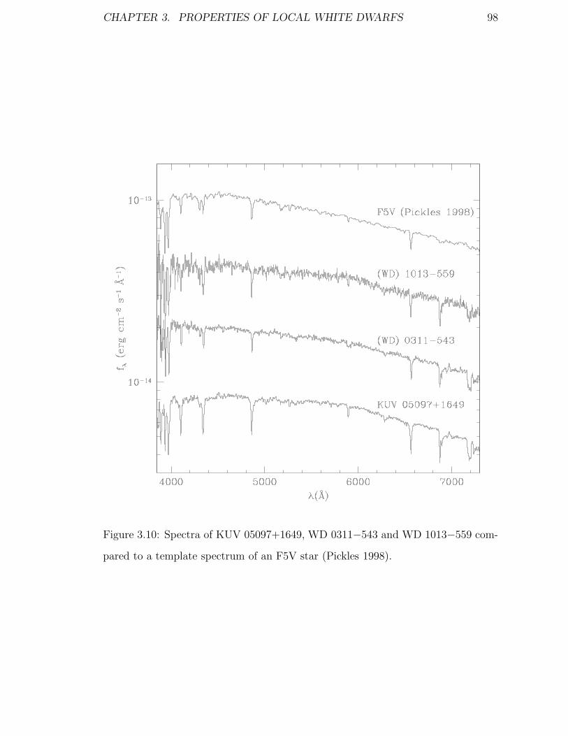
CHAPTER 3. PROPERTIES OF LOCAL WHITE DWARFS 98
Figure 3.10: Spectra of KUV 05097+1649, WD 0311−543 and WD 1013−559 com-
pared to a template spectrum of an F5V star (Pickles 1998).
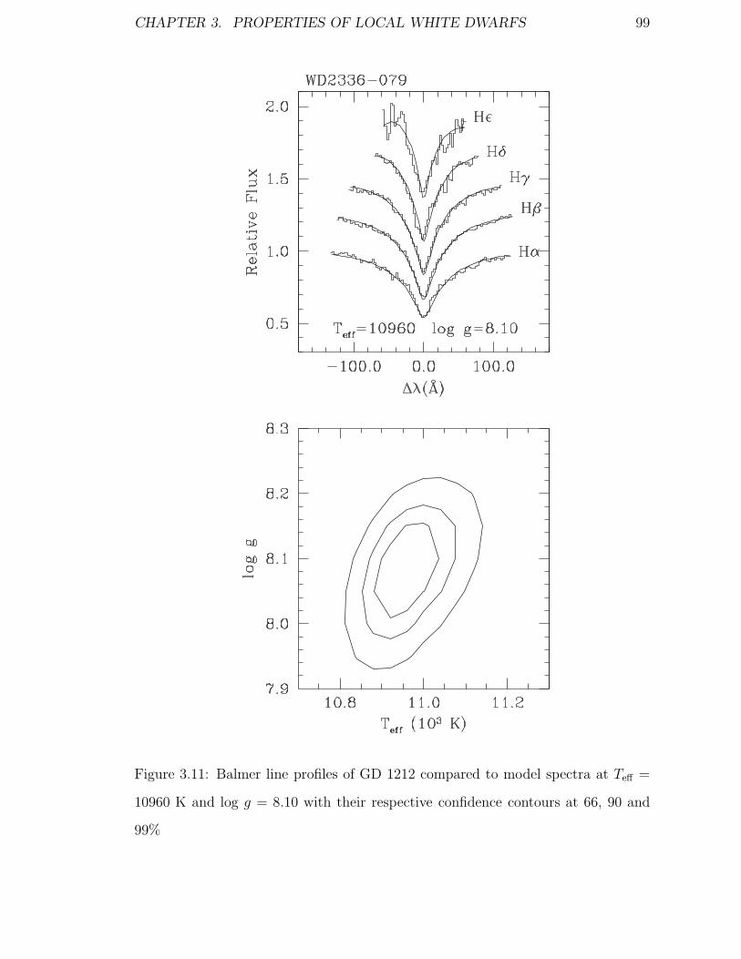
CHAPTER 3. PROPERTIES OF LOCAL WHITE DWARFS 99
Figure 3.11: Balmer line profiles of GD 1212 compared to model spectra at Teff =
10960 K and log g = 8.10 with their respective confidence contours at 66, 90 and
99%

CHAPTER 3. PROPERTIES OF LOCAL WHITE DWARFS 100
Table 3.7: Reclassification of stars
WD Other Name Old Type New Type Reference
0311−543 BPM 17113 DZ7 F5V 1
0509+168 KUV 05097+1649 DA F2V 2
1013−559 BPM 19929 DZ9 F3V 3
1717−345 SC 1717−3430 DA DA+dMe 4
2336−079 GD 1212 DA DA4.5 5
REFERENCES: (1) Wegner (1975); (2) Wegner & McMahan
(1988); (3) Wegner (1973a); (4) Reid et al. (1988); (5) Berger &
Fringant (1984)
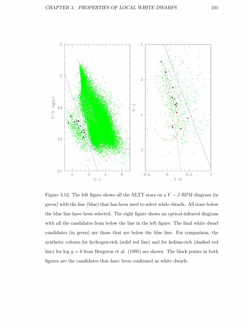
CHAPTER 3. PROPERTIES OF LOCAL WHITE DWARFS 101
Figure 3.12: The left figure shows all the NLTT stars on a V − J RPM diagram (in
green) with the line (blue) that has been used to select white dwarfs. All stars below
the blue line have been selected. The right figure shows an optical-infrared diagram
with all the candidates from below the line in the left figure. The final white dwarf
candidates (in green) are those that are below the blue line. For comparison, the
synthetic colours for hydrogen-rich (solid red line) and for helium-rich (dashed red
line) for log g = 8 from Bergeron et al. (1995) are shown. The black points in both
figures are the candidates that have been confirmed as white dwarfs.

CHAPTER 3. PROPERTIES OF LOCAL WHITE DWARFS 102
Table 3.8: Motion and colours of newly discovered white dwarfs
Name WD µ, θ vrad V V − J J − H H − K
NLTT (” yr−1, ◦) (km s−1) (mag) (mag) (mag) (mag)
529 0008+423 0.237, 193 69 15.2 ± 0.2 0.69 0.236 -0.094
8435 0233−242 0.622, 189 (0) 15.74 ± 0.07 1.28 0.145 0.145
8581 0236+259 0.362, 119 28 16.2 ± 0.2 1.31 0.332 0.117
19138 0810+489 0.258, 167 (0) 15.1 ± 0.2 0.76 0.232 0.002
31748 1242−105 0.349, 257 70 14.7 ± 0.2 0.48 0.163 -0.025
40607 1532+129 0.248, 221 -38 15.07 ± 0.05 0.94 0.246 -0.021
49985 2048−250 0.278, 130 51 15.60 ± 0.53 0.65 0.197 0.087
52404 2152−280 0.234, 44 (0) 16.26 ± 0.17 0.91 0.210 0.179
53177 2209−147 0.267, 70 24 15.090 ± 0.015 0.55 0.143 0.184
53468 2215−204 0.249, 72 49 15.3 ± 0.2 -0.60 -0.083 0.372
55932 2306−220 0.339, 106 56 13.68 ± 0.06 -0.59 0.010 -0.162
56805 2322+137 0.353, 72 53 16.1 ± 0.2 1.63 0.159 -0.030

CHAPTER 3. PROPERTIES OF LOCAL WHITE DWARFS 103
Figure 3.13: Spectra of the new DA white dwarfs and the confirmed DA white dwarf
WD 2336−079 in order of decreasing temperature.
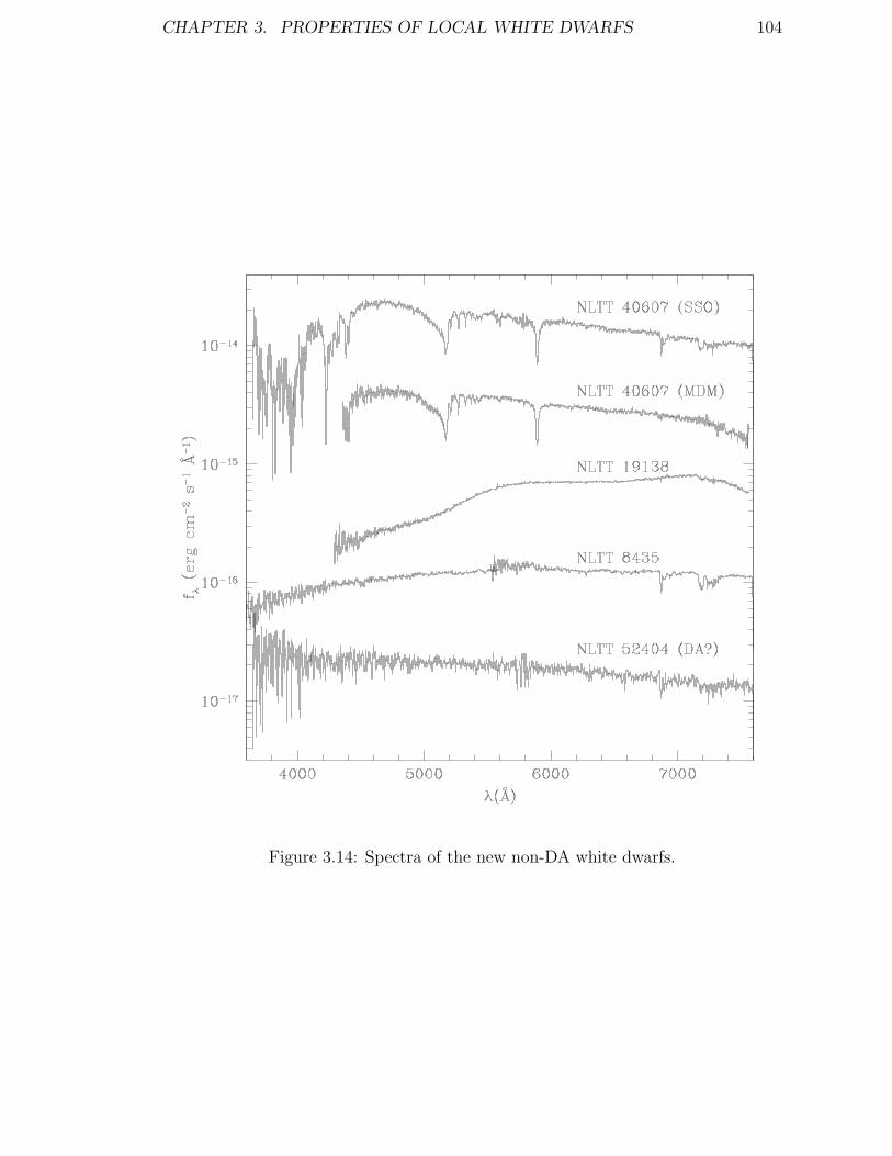
CHAPTER 3. PROPERTIES OF LOCAL WHITE DWARFS 104
Figure 3.14: Spectra of the new non-DA white dwarfs.

CHAPTER 3. PROPERTIES OF LOCAL WHITE DWARFS 105
Figure 3.15: Balmer line profiles of NLTT 529 compared to pure-hydrogen model
spectra with the confidence contours for the fit at 66, 90 and 99%.
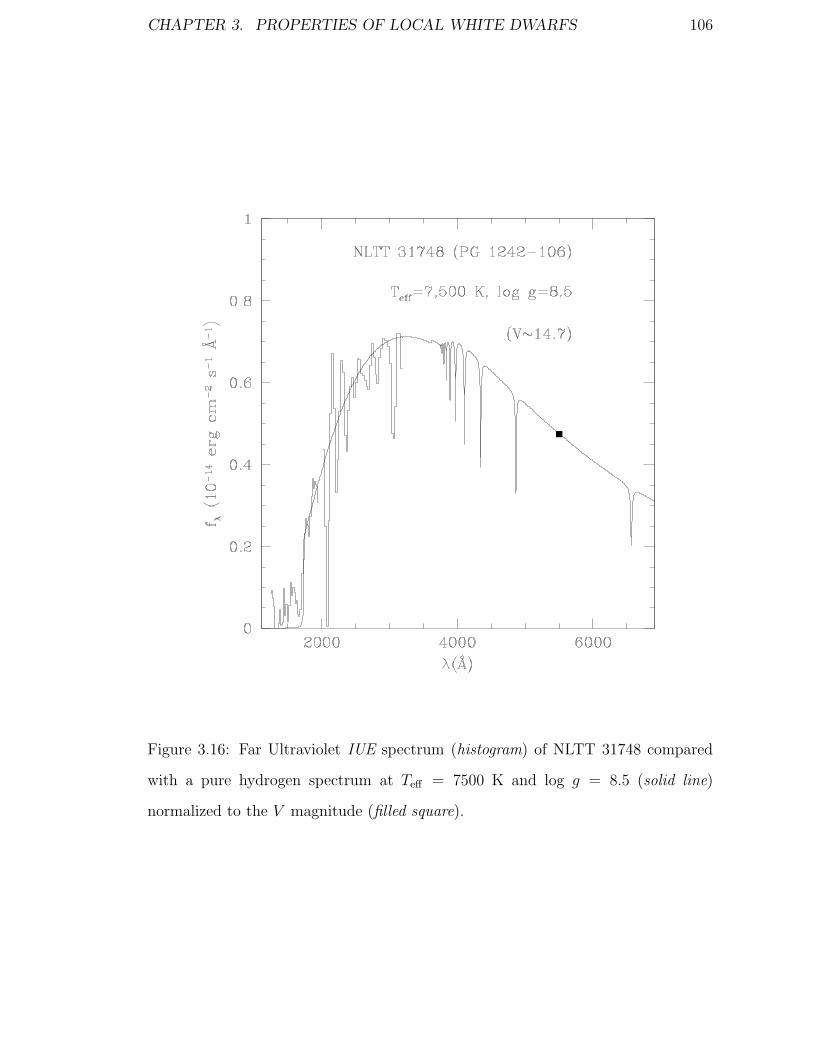
CHAPTER 3. PROPERTIES OF LOCAL WHITE DWARFS 106
Figure 3.16: Far Ultraviolet IUE spectrum (histogram) of NLTT 31748 compared
with a pure hydrogen spectrum at Teff = 7500 K and log g = 8.5 (solid line)
normalized to the V magnitude (filled square).

CHAPTER 3. PROPERTIES OF LOCAL WHITE DWARFS 107
Figure 3.17: Balmer line profiles of NLTT 31748 from MSO (left) and from SSO
(right) compared to model spectra with their respective confidence contours at 66,
90 and 99%

CHAPTER 3. PROPERTIES OF LOCAL WHITE DWARFS 108
Figure 3.18: Spectrum of NLTT 40607 showing the absorption due to Ca I, Mg I,
Fe I and Na I. The bottom spectrum shows the line identifications.

CHAPTER 3. PROPERTIES OF LOCAL WHITE DWARFS 109
Figure 3.19: Balmer line profiles of NLTT 49985 compared to pure-hydrogen model
spectra with the confidence contours for the fit at 66, 90 and 99%.

CHAPTER 3. PROPERTIES OF LOCAL WHITE DWARFS 110
Figure 3.20: Balmer line profiles of NLTT 53177 compared to pure-hydrogen model
spectra with the confidence contours for the fit at 66, 90 and 99%.

CHAPTER 3. PROPERTIES OF LOCAL WHITE DWARFS 111
Figure 3.21: Balmer line profiles of NLTT 53468 compared to pure-hydrogen model
spectra with the confidence contours for the fit at 66, 90 and 99%.

CHAPTER 3. PROPERTIES OF LOCAL WHITE DWARFS 112
Figure 3.22: Balmer line profiles of NLTT 55932 compared to pure-hydrogen model
spectra with the confidence contours for the fit at 66, 90 and 99%.

CHAPTER 3. PROPERTIES OF LOCAL WHITE DWARFS 113
Tab
le3.
9:Par
amet
ers
and
kin
emat
ics
ofnew
lydis
cove
red
whit
edw
arfs
Nam
eSpec
tral
Type
Com
pos
itio
nT
efflo
ggM
MV
dU,V
,W
K(c
.g.s
.)(M
�(m
ag)
(pc)
(km
s−1)
NLT
T52
9D
AH
7420
±10
08.
15±
0.05
0.69
±0.
0313
.522
-5,61
,-3
7
NLT
T84
35D
CH
e53
00±
200
(8.0
)(0
.58)
14.7
1646
,-2
2,0
NLT
T85
81D
AH
5500
±50
0(8
.0)
(0.5
8)14
.621
-27,
-12,
-6
NLT
T19
138
DC
He
6200
+1500
−900
(8.0
)(0
.58)
14.0
178,
-15,
9
NLT
T31
748
DA
H80
00±
200
8.00
±0.
500.
68±
0.06
13.0
222,
-56,
56
NLT
T40
607
DZ
Mg,
Fe,
Na,
He?
∼75
00(8
.0)
(0.5
8)13
.224
-8,-3
0,-1
6
NLT
T49
985
DA
H76
00±
100
9.00
±0.
031.
24±
0.02
14.2
1839
,6,
-40
NLT
T52
404
DC
He
6500
±50
0(8
.0)
(0.5
8)13
.831
-14,
26,-4
NLT
T53
177
DA
H80
40±
608.
26±
0.15
0.76
±0.
1013
.323
-4,21
,-2
3
NLT
T53
468
DA
H15
800±
250
7.80
±0.
080.
51±
0.04
10.9
76-4
5,31
,-7
4
NLT
T55
932
DA
H15
120±
120
7.85
±0.
050.
53±
0.03
11.1
33-1
0,-9
,-6
5
NLT
T56
805
DA
H47
00±
300
∼7.
0...
14.4
22-2
8,37
,-3
3

CHAPTER 3. PROPERTIES OF LOCAL WHITE DWARFS 114
3.6.2 Kinematics
The kinematical properties of the observed white dwarfs in the previous section are
summarized in Table 3.9. The velocity components U , V and W were computed us-
ing Johnson & Soderblom (1987), where U , V and W represent the space velocities
in the direction of the Galactic centre, the Galactic rotation, and the North Galactic
pole, respectively. U , V and W components were also calculated for all 417 white
dwarf candidates, which were selected using their proper motion and infrared-optical
colours as discussed in section 3.6.1. In the calculation of the velocity components
for these objects, the radial velocity was assumed to be zero. All three distri-
butions were fitted with gaussian functions where (σU , σV , σW ) = (41, 23, 22) and
(〈U〉, 〈V 〉, 〈W 〉) = (1,−21,−2), which is in agreement with Anselowitz et al. (1999),
with the exception of the V distribution which appears somewhat narrower. The
average velocity component 〈V 〉 = −21 is markedly more negative than the velocity
component of normal stars in the thin disk (1998, 〈V 〉 = −6 km s−1) which sug-
gested that the white dwarfs are part of the ”old thin disk” (Sion et al., 1988). The
integrated area of the gaussian fit to the V distribution corresponds to only 395 ob-
jects. The V distribution shows an extended tail of ∼ 22 high-velocity objects near
V = −70,−120 km s−1. Finally, the gaussian fit to the W distribution corresponds
to 408 objects. Therefore at least 395 objects, out of 417, appear to belong to the
same population, that is they belong to the thin disk.
Figure 3.26 shows the measurements in the U versus V plane. The measurements
are compared to velocity ellipses, and, as noted above, most objects belong to the
thin disk. Chiba & Beers (2000) determined (σU , σV , σW ) = (141, 106, 94) and
〈V 〉 = −187 for halo stars based on the kinematics of metal-poor stars, and also
determined (σU , σV , σW ) = (46, 50, 35) and 〈V 〉 = −20 for thick disk stars.
There are 344 objects residing inside the 2σ thin disk ellipse described by the
relations: ( U
2σU
)2
+( V
2σV
)2
< 1

CHAPTER 3. PROPERTIES OF LOCAL WHITE DWARFS 115
Figure 3.23: Spectra of newly identified white dwarfs compared with the known DA
LHS 1415 (left). Details of Hα line profiles reveal that NLTT 8435 is He-rich. The
spectra are compared with synthetic spectra. The spectra, in particular NLTT 8581,
show strong telluric absorption features.

CHAPTER 3. PROPERTIES OF LOCAL WHITE DWARFS 116
Figure 3.24: Optical B − V and U − B diagram showing available photometry for
the observed local white dwarfs, compared to a pure hydrogen sequence at log g = 8
and the main sequence (in red).

CHAPTER 3. PROPERTIES OF LOCAL WHITE DWARFS 117
Figure 3.25: Optical-infrared V −J and J−H diagram showing 2MASS photometric
measurements compared with synthetic colours from Bergeron et al. (1995). The
pure hydrogen sequence at log g = 8 and the measurements are displayed as solid
lines, and the pure helium sequence and the data are displayed as dashed lines. The
curves are labeled with the effective temperature in units of 1000 K.

CHAPTER 3. PROPERTIES OF LOCAL WHITE DWARFS 118
or ( U
σU
)2
+( V
σV
)2
< 4
where U and V have been centred on their mean values. Both distributions in U/σU
and V/σV are normalized. The combined distribution is a bivariate normal density
distribution. The probability of finding thin disk objects within the 2σ ellipse is
given by integrating the probability density function inside the ellipse:
P(( U
σU
)2
+( V
σV
)2
< 4)
=1
2π
∫ 2
−2
e−u2/2
∫ √4−u2
−√4−u2
e−v2/2dvdu
or
P (2σ) = 0.8646.
where u = U/σU and v = V/σV . Assuming that 395 objects are genuine thin disk
members, then there should be 342 of them residing within the 2σ ellipse in, which
is in agreement with the data, i.e., 344 objects are found within the 2σ ellipse. It
would therefore appear that only 22 objects from the sample belong to either the
thick disk or the halo. The white dwarf WD2316−065 is already recognized as a halo
candidate (Liebert et al., 1989). Two objects in Figure 3.26 reside within the 1σ halo
region at the exclusion of all other regions, and are also excellent halo candidates
(NLTT 8733, and NLTT 32057=WD1247+550). Overall, ≈ 5% of the sample may
belong to the thick disk, and ≈ 1% to the halo.
Recently, Pauli et al. (2003) proposed that a very high fraction of 4% of white
dwarfs belong to the halo. Most objects from their selection are young. The lumi-
nosity function for halo white dwarfs (Liebert et al., 1989; Hansen, 2001) is likely to
peak at very low luminosity and the fraction of luminous halo candidates in the sam-
ple of Pauli et al. (2003) might imply, when extrapolated to lower luminosity, that
all cool white dwarfs are halo members. Another explanation is that the peculiar
velocity of some white dwarfs may be the result of past binary interaction.

CHAPTER 3. PROPERTIES OF LOCAL WHITE DWARFS 119
Figure 3.26: U versus V diagram showing 417 colour-selected rNLTT white dwarfs.
The 2σ velocity ellipse of the identified thin disk population is shown (full line) along
with the 2σ ellipse of the thick disk (short dashed line), and the 1σ ellipse of the
halo (long dashed line) populations. The halo candidate LHS 542 (WD 2316−065)
is marked.

CHAPTER 3. PROPERTIES OF LOCAL WHITE DWARFS 120
3.6.3 Discussion
In this section on the local population of white dwarfs I found that 17% of white
dwarfs have magnetic fields, which is significantly higher than previously believed.
However, the previous estimates of the incidence of magnetism in white dwarfs
were based on magnitude limited surveys. For example only 2% of white dwarfs
were found to be magnetic in the Palomar-Green survey (Liebert et al., 2003), and
Schmidt & Smith (1995) found that about 4% of white dwarfs are magnetic. How-
ever, magnitude limited surveys tend to favour less massive white dwarfs and there-
fore they are more likely to be biased against the generally more massive magnetic
white dwarfs. Moreover, the local population of white dwarfs is much older than the
white dwarfs selected in the Palomar-Green survey. The incidence of magnetism in
white dwarfs appears to be higher in cooler white dwarfs.
In order to ascertain the spectral classification of all known white dwarfs within
20 pc of the Sun, five stars from the list of Holberg, et al. (2002) were observed.
Three of these stars were found not to be white dwarfs, but rather F-type stars.
One of these was confirmed to be a DA white dwarf and another was found to be a
distant DA plus dMe binary. Note that removing three stars from the white dwarf
list of Holberg, et al. (2002) reduces the local density of white dwarf stars by ≈ 6%.
A revised estimate of the local density would be 4.7± 0.7× 10⁻³ pc−3, which is not
significantly lower than the original estimate.
I have used the revised NLTT catalog (Salim and Gould, 2003) to select 417
white dwarf candidates. The candidates were selected on the basis of their proper
motion and optical/infrared colours. About half of these candidates have already
been spectroscopically confirmed as white dwarfs. From the remaining half, 12 new
white dwarfs have been spectroscopically identified, with three of these lying within
20 pc of the Sun. Eight of these stars were found to be hydrogen rich white dwarfs,
three of them are of the spectral type DC, and therefore are helium rich, and finally
one of the new white dwarfs was found to be a DZ white dwarf. All except two

CHAPTER 3. PROPERTIES OF LOCAL WHITE DWARFS 121
of these white dwarfs are cooler than 10000 K, and one white dwarf was found to
be an ultramassive white dwarf (NLTT 49985), which are relatively rare in optical
selections (Vennes, 1999).
Kinematics of the sample of rNLTT white dwarf candidates suggest that about
94% of these stars belong to the thin disk, with the remaining 6% belonging to the
thick disk or the halo. The kinematics of the twelve observed white dwarfs place
them into the thin disk.
3.7 Summary
The properties of the local population of white dwarfs have been studied. The spec-
tropolarimetric survey of hydrogen-rich white dwarfs in the southern hemisphere did
not find any new magnetic white dwarfs, however it was useful in constraining the
incidence of magnetism in the Solar neighbourhood, which is about 17%. Further-
more, I have used the revised NLTT catalog to search for new nearby white dwarfs.
A total of 417 candidates were selected out of which about half have been previously
spectroscopically confirmed as white dwarfs. An additional 12 new spectroscopically
identified white dwarfs can be added to this list. The preliminary work on the NLTT
survey suggests that the sample of white dwarfs with distances d < 13 pc listed by
Holberg, et al. (2002) is complete, but that more objects with distances 13 < d < 20
pc remain to be discovered.

Chapter 4
Close Binary Systems
4.1 Introduction
Observations have been carried out for the four close binaries BPM 71214, EUVE
J0720−31.7, BPM 6502 and EC 13471−1258. The orbital periods range from 3.6
hours to 1.26 days. Three of these systems have been known to be close binaries,
but BPM 6502 was discovered to be a close binary during observations carried out
for this project. The observations of these four binaries will be presented in this
chapter, which allowed the determination of ephemerides for all of these binaries,
along with atmospheric parameters of the white dwarfs.
BPM 71214 is a poorly studied close binary that has been classified as a post-
common envelope binary by Hillwig, Honeycutt & Robertson (2000) and as a pre-
cataclysmic variable by Marsh (2000). Livio & Shara (1987) and Sarna, Marks &
Smith (1995) suggested that BPM 71214 may be a possible hibernating nova. A
period of 4 hr 20 minutes was quoted by Livio & Shara (1987), however Marsh
(2000) quoted a period of 0.202 days (∼ 4 hr 51 min).
EUVE J0720−31.7 is a post-common envelope binary, which was discovered in
the Extreme Ultraviolet Explorer (EUVE) all-sky survey by Vennes & Thorstensen
(1994a). They observed a hot hydrogen-rich white dwarf spectrum with overlying
122

CHAPTER 4. CLOSE BINARY SYSTEMS 123
narrow Balmer-line emission, a sign that the white dwarf has a close late-type com-
panion. Later observations of the white dwarf revealed the presence of optical helium
and ultraviolet helium and carbon in its spectrum (Barstow et al. (1995b), Vennes,
Thorstensen & Polomski (1999b)), giving this white dwarf a DAO classification. The
atmospheric parameters of the white dwarf have been determined by Finley, Koester
& Basri (1997), Marsh et al. (1997) and Vennes et al. (1997). The effective tem-
perature measurements ranged from 52400 to 55100 K and the surface gravity (log
g) ranged from 7.64 to 7.92. These measurements were then used to determine the
mass of the white dwarf, from 0.51 to 0.67 M�. An ephemeris for this binary system
was determined by Vennes & Thorstensen (1996), which was later used to phase
observations of the system using the Hubble Space Telescope (HST) Goddard High-
Resolution Spectrograph. With these observations Vennes, Thorstensen & Polomski
(1999b) were able to measure the photospheric abundances of helium and carbon,
and using the spectral lines of He II λ1640 and C IV λ1550, they were able to trace
the orbital motion of the white dwarf.
BPM 6502 is a high-proper motion star which was observed as part of the Bruce
Proper Motion Survey (Luyten, 1963), and has also been identified as LTT 3943 in
the catalog of proper-motion stars exceeding 0.′′2 annually (Luyten, 1957). BPM 6502
was listed as a white dwarf candidate by Eggen (1969). Wegner (1973b) confirmed
it as a white dwarf spectroscopically and catalogued it as WG 17. Atmospheric
parameters were estimated for the white dwarf by Koester, Schulz & Weidemann
(1979) and Bragaglia, Renzini & Bergeron (1995). The effective temperature was
estimated to be between 19,800 and 21,600 K and the surface gravity close to log
g = 8. The aim of the observations of Bragaglia et al. was to discover double
degenerate systems (Bragaglia et al., 1990), however no significant radial velocity
variations were reported in the case of BPM 6502.
EC 13471−1258 is an eclipsing close binary that was observed as part of the
Edinburgh-Cape Blue Object Survey (Kilkenny et al., 1997). Kilkenny et al. (1997)

CHAPTER 4. CLOSE BINARY SYSTEMS 124
classified the system as a DA plus dM binary and measured and orbital period of 3
hr 37 minutes from photometry. They also observed some flaring of the dM star. A
recent study of EC 13471−1258 has been presented by O’Donoghue et al. (2003).
In this chapter, the spectroscopic and photometric observations of the close bi-
nary stars BPM 71214, EUVE J0720−31.7, BPM 6502 and EC 13471−1258 will be
presented. First, the required theory to measure orbital parameters is presented in
section 4.2. In section 4.3 details of the observations are presented. The data reduc-
tion and results for the four binaries are presented in section 4.4. I will summarize
the results in section 4.5.
4.2 Measuring Orbital Parameters
The orbital motion of the secondary star in many DA plus dMe binaries can be traced
by a velocity shift of hydrogen emission lines that originate from its surface. Balmer
emission lines can be observed if the secondary star has an active chromosphere. Also
the emission lines can be the result of reprocessing of extreme ultraviolet (EUV) or
far-ultraviolet (FUV) radiation from the white dwarf in the atmosphere of the red
dwarf. If the emission is purely a result of the reprocessing of EUV and/or FUV
radiation then the equivalent width (EW ) will vary with the orbital motion, since
only the closer half of the red dwarf will be illuminated by the white dwarf.
The amount of variation in the equivalent width of the hydrogen emission line
that is the result of reprocessing in the secondary atmosphere can be used to ap-
proximate the inclination of the system. Thorstensen et al. (1978) modeled the
equivalent width variations as a function of the orbital phase. In their models they
assume that all the emission is associated with the red dwarf, that the emitting
region is confined to a layer that is much smaller than the radius of the red dwarf,
and that the emission is entirely due to radiation reprocessing, meaning that none
of it is intrinsic to the red dwarf. Adopting these three basic assumptions, they

CHAPTER 4. CLOSE BINARY SYSTEMS 125
develop three models. The three models proposed differ in the assumptions made
concerning the optical thickness of the emitting layers in the red dwarf, and the
depth of the emitting layer. Model A assumes:
• the emitting layer is optically thin to the emerging Hα radiation,
• and each EUV photon will result in the emission of f photons of Hα radiation.
The value of f is calculated by assuming that the number of recombinations of
hydrogen to levels with n ≥ 2 be equal in each column to the incoming EUV
photon flux.
Model B differs from model A only in assuming that the Hα optical depth is very
large, which would result in the Hα surface brightness of the illuminated hemisphere
being constant. Model C differs from A and B, in that the emitting layer is assumed
to be optically thick in Hα.
If the equivalent width variation is known, then the fraction of the minimum
EW to the maximum EW can be used to approximate the inclination of the system.
Using the equations of Thorstensen et al. (1978) for model A/B, then:
sin i =1 − x
1 + x, (4.1)
where x is the fraction EWmin/EWmax. If there is any intrinsic Hα emission from
the red dwarf, then this needs to be considered, and therefore equation 4.1 cannot
be used as it is. Examples of such systems are PG 1026+002 (Bruch and Diaz, 1999;
Saffer et al., 1993), RR Cae (Bruch, 1999), and PG 0308+096 (Saffer et al., 1993;
Somers et al., 1996).
If the emission is intrinsic to the red dwarf then the emission traces the orbital
path of the centre of mass of the red dwarf. However, if the emission is due to
the reprocessing of EUV or FUV radiation, then the Hα emission traces a lower
orbit than the true centre of mass orbit. The reason for this is that the white
dwarf only illuminates the exposed half of the red dwarf surface. For example in

CHAPTER 4. CLOSE BINARY SYSTEMS 126
the close binary Feige 24, Vennes & Thorstensen (1994b) measured radial velocities
of the red dwarf using TiO absorption bands and Hα emission lines. They found
that the radial velocity amplitude of the red dwarf determined from the Hα radial
velocities is systematically 3.9 km s−1 lower than the amplitude measured using
TiO absorption bands. The radial velocity measurements due to Hα emission can
be corrected to represent the true centre of mass orbital path. Vennes, Thorstensen
& Polomski (1999b) derived an approximate formula which first requires an estimate
of the binary separation using Kepler’s third law:
P 2orb =
4π2a3
G(MRD + MWD)=
4π2a3
GMWD(1 + q), (4.2)
where a is the separation between the centres of mass of the two binary components,
and Porb is the orbital period of the binary. This equation can be used to calculate
the separation of the system. Initially the mass ratio can be approximated using
the uncorrected red dwarf radial velocity semi-amplitude where:
q =MRD
MWD
=KWD
KRD
. (4.3)
KWD and KRD are the radial velocity semi-amplitudes of the white dwarf and red
dwarf, respectively. Using the mass ratio, the red dwarf semi-major axis can be
estimated with aRD = a(1+q)
, which is then used to obtain a new KRD,corr:
KRD,corr = KRD(1 − 0.4RRD
aRD)−1 (4.4)
The factor aRD/(aRD − 0.4RRD) is the ratio of the red dwarf semi-major axis to the
reduced red dwarf semi-major axis, where 0.4RRD is the assumed distance from the
centre of the red dwarf to the centre of the illuminated hemisphere.
If the binary is eclipsing, then it is possible to calculate an approximate inclina-
tion, based on the radius of the secondary and the length of time the white dwarf
is eclipsed by the red dwarf.
sin2 i ≈ 1 − (RRD
a)2
cos2(πϕp), (4.5)
CHAPTER 4. CLOSE BINARY SYSTEMS 127
where ϕp is the length of the eclipse and RRD is the radius of the secondary. This
is only an approximate equation because it assumes the secondary to be a sphere
rather than the distorted shape of a star that is filling its Roche lobe (Warner, 1995).
4.3 Observations
4.3.1 Optical Spectroscopy and Photometry
The spectroscopic observations of the four studied close binaries were all conducted
at the 74 inch telescope (1.9m) at the Mount Stromlo Observatory (MSO). Pho-
tometric observations of these objects were conducted at MSO and at the 24 inch
Perth/Lowell Boller & Chivens Cassegrain reflector (f/13.5) at the Perth Observa-
tory (Perth). The observations at the MSO used the SITE 1752 × 532 CCD for
observations conducted in 2000 and the 2048 × 4096 CCD for the remaining ob-
servations. All images were binned 2 × 2. Table 4.1 and Table 4.2 give the dates
and setup of the observations. The data for EUVE J0720−31.7 prior to March 2000
were obtained by Stephane Vennes.
The images of BPM 6502 were reduced with DoPhot (Schechter et al., 1993) by
Andrew Williams of Perth Observatory where all stars in the images were measured.
A set of 7 reference stars were chosen, and their fluxes summed to form reference
magnitudes for each image for both I and R filters. These were subtracted from
each measurement of BPM 6502, to minimize any external effects causing variations
between exposures. The overall average of these differential magnitudes is used
as the photometric zero-point for the light curve, calculated for I and R bands.
Figure E.1 shows one of the images taken using the R filter with BPM 6502 and the
reference stars marked.
The images of EC 13471−1258 are 3.0 × 3.3 arc minutes and have a resolution
of 0.546 arc sec per binned pixel. The images of BPM 71214 are 3 × 6 arc minutes
and have a resolution of 0.546 arc seconds per binned pixel. Figure E.1 shows the

CHAPTER 4. CLOSE BINARY SYSTEMS 128
Table 4.1: Observations - Spectroscopy
Object Date Grating Exp. Time
(s)
BPM 71214 2002 February 12,13 7500 A 1200 line/mm 600
2002 February 14 5000 A 300 line/mm 1200
2002 February 14 7500 A 1200 line/mm 900
2002 March 1,2 7500 A 1200 line/mm 600/900
2002 March 7,8 7500 A 1200 line/mm 600
2002 March 10 7500 A 1200 line/mm 900
2002 March 30,31 5000 A 300 line/mm 600
2002 September 15 7500 A 1200 line/mm 600
EUVE J0720−31.7 1999 October 10 7500 A 1200 line/mm 1800
1999 November 10-15 7500 A 1200 line/mm 2400
2000 February 4-9 7500 A 1200 line/mm 1800
2000 March 1,31 7500 A 1200 line/mm 1800
2002 April 5,6,7,15 5000 A 300 line/mm 1800
BPM 6502 2000 March 2,3,9-11 7500 A 1200 line/mm 1800
2000 March 30,31 7500 A 1200 line/mm 1800
2000 April 3,5,6 7500 A 1200 line/mm 1800
2002 January 26,27 7500 A 1200 line/mm 1800
2002 February 1,11 7500 A 1200 line/mm 1800
2002 March 1 7500 A 1200 line/mm 1800
2002 March 5 5000 A 300 line/mm 600
2002 March 10 5000 A 300 line/mm 1200
2002 March 30 5000 A 300 line/mm 600
EC 13471−1258 2002 March 1 7500 A 1200 line/mm 1200
2002 March 8 7500 A 1200 line/mm 1200
2002 March 8 5000 A 300 line/mm 600
2002 March 9 7500 A 1200 line/mm 900
2002 March 10 5000 A 300 line/mm 600
2002 March 31 5000 A 300 line/mm 240/600
2002 April 1 5000 A 300 line/mm 120/600
2002 April 5,6 5000 A 300 line/mm 120
2002 April 15 5000 A 300 line/mm 300

CHAPTER 4. CLOSE BINARY SYSTEMS 129
Table 4.2: Observations - Photometry
Object Telescope Date Filter Exp. Time (s)
BPM 71214 MSO 2002 September 17,19,20 R 20
MSO 2002 September 21 I 4
BPM 6502 Perth 2001 October 9,10 R,I 120
Perth 2001 October 18-23 R,I 120
EC 13471−1258 MSO 2002 April 18,19,21 B,R 20

CHAPTER 4. CLOSE BINARY SYSTEMS 130
locations of BPM 71214 and EC 13471−1258 with their respective comparison stars
which were used in obtaining a reference magnitude. The comparison stars were
checked for non-variability. These images were reduced using the routine QPHOT
in the IRAF APPHOT package.
4.3.2 Archival Ultraviolet Data
A short-wavelength International Ultra-violet Explorer (IUE) spectrum (SWP 27251)
and a long-wavelength spectrum (LWP 07351) of BPM 6502 were obtained from the
Multimission Archive at the Space Telescope Science Institute where the NEWSIPS
spectra were chosen (1996).
EC 13471−1258 was observed with the HST Goddard High-Resolution Spectro-
graph by D. O’Donoghue, who obtained 17 exposures on 1999 August 28. A set of
two 300 s exposures were taken using the NUV-MAMA configuration with a spec-
tral coverage of 1568 to 3184 A and a resolution of 3.4 A. The G230L filter centred
at 2376 A with a bandwidth of 1616 A was used. A total of 15 exposures of 300
second duration were obtained using the FUV-MAMA configuration with a spectral
coverage of 1140 to 1730 A and a resolution of 1 A. For these exposures the G140L
filter centred at 1425 A with a bandwidth of 590 A was used.
BPM 71214 and EC 13471−1258 have been observed with ROSAT as 1RXS
J033243.5−085531 and 1RXS J134951.0−131338, respectively. BPM 71214 has been
found to be an X-ray source with a count rate of 0.079 ± 0.02 counts per second
and EC 13471−1258 was found to be an X-ray source with a count rate of 0.14 ±0.02 counts per second. Both X-ray sources have a hardness ratio that suggest the
possibility of accretion onto the white dwarf or, more likely, the presence of coronal
activity.

CHAPTER 4. CLOSE BINARY SYSTEMS 131
4.4 Analysis
4.4.1 BPM 71214
Orbital Parameters
The Hα radial velocity measurements for BPM 71214 are shown in Table E.1. The
radial velocity measurements marked with an asterix were measured from low dis-
persion spectra. For the calculation of the period these velocities had a reduced
weight (0.25) compared to the radial velocities obtained from high dispersion spec-
tra. Figure 4.1 shows the periodogram of Hα radial velocity measurements, with
the velocities folded on the best orbital period of:
P = 0.201626 ± 0.000004 d,
with the epoch of inferior conjunction:
T0 = 2452318.102± 0.004 (HJD).
The radial velocity semi-amplitude of the red dwarf is 123.6 ± 2.1 km s−1 and the
systemic velocity is 46.2 ± 1.5 km s−1. The mass function of the white dwarf is
0.039±0.002 M�, and it differs significantly from the mass function quoted in Livio
& Shara (1987) of 0.20, which is therefore in error. The mass function and probable
mass of the components (see below) suggest a system inclination of i ∼ 30◦.
The Hα equivalent width did not appear to vary over the orbital period (E.W.∼6.0A) despite model expectations of about 50% (i.e., ≈ sin i), therefore the Hα
emission is due to coronal activity and not to an illumination effect. The Hα emission
is therefore distributed over the entire surface of the star and the inferred orbital
parameters are representative of the motion of the red dwarf centre of mass. To
check that this is the case, the absorption features in the wavelength range 6240 to
6540 A were used to obtain radial velocity measurements. The absorption features
in BPM 71214 were compared to GL 250B (M2 star: observed on 2002 March 8
using the same setup as BPM 71214) using the IRAF routine FXCOR to obtain

CHAPTER 4. CLOSE BINARY SYSTEMS 132
Figure 4.1: The radial velocity of the red dwarf in BPM 71214 traced by Hα and
folded on the orbital period and best fit (bottom), and the period analysis (top).The
full line shows the 90% confidence level and the dashed line shows the 99% confidence
level of the orbital period.

CHAPTER 4. CLOSE BINARY SYSTEMS 133
Figure 4.2: The radial velocity traced by absorption features for BPM 71214 in the
wavelength range 6240 to 6540 A and folded on the orbital period compared to the
best sinusoidal fit, which has a semiamplitude of 116.2±2.5 km s−1 and an systemic
offset of 45.8 ± 1.8 km s−1.

CHAPTER 4. CLOSE BINARY SYSTEMS 134
relative radial velocities. The radial velocity of GL 250B (-8 km s−1: Stauffer &
Hartmann (1986)) was subtracted from the heliocentric corrected velocities of BPM
71214. Figure 4.2 shows the absorption radial velocity measurements folded on
the best orbital period compared to the best fit sinusoid with a semi-amplitude of
116.2 ± 2.5 km s−1 and a systemic velocity of 45.8 ± 1.8 km s−1. The absorption
radial velocity measurements are given in Table E.2. These two values agree with
the semi-amplitude and systemic velocity determined using the Hα emission within
the 1σ errors. Therefore, the Hα emission appears to trace the orbit of the red dwarf
centre of mass. Note that the source of X-rays is related to coronal activity.
Spectral Decomposition
A white dwarf spectrum of BPM 71214 was obtained by subtracting a series of late-
type spectra from the observed low-dispersion spectrum until the TiO bands are not
observed from the resulting spectrum. Pickles (1998) provides a library of spectra
that represent M-type stars, and were used in the decomposition of the observed
BPM 71214 spectrum.
Figure 4.3 shows the decomposed spectrum of the white dwarf and the red dwarf
in BPM 71214 based on a series of low dispersion spectra. The spectrum of the red
dwarf was compared to the series of template spectra for M dwarfs, with the M2.5V
spectral type being the best fit. The white dwarf spectrum which was obtained from
the subtraction of the template red dwarf spectrum from the observed spectrum,
was compared to a grid of model spectra to obtain Teff = 17200 ± 1000 K and
log g = 8.20 ± 0.10. Figure 4.4 shows the Balmer line profiles of the white dwarf
after decomposition compared to the best fit synthetic spectrum with confidence
contours for the fit. The mass of the white dwarf is 0.77 ± 0.06M� with a cooling
age of 2.15±0.37×10⁸ years, which has been calculated using Wood (1995) models.

CHAPTER 4. CLOSE BINARY SYSTEMS 135
Figure 4.3: The decomposed spectrum of BPM 71214. The top panel shows the
white dwarf spectrum compared to a model spectrum (blue). The bottom panel
shows the red dwarf spectrum compared to a dM2.5 template (Pickles 1998).

CHAPTER 4. CLOSE BINARY SYSTEMS 136
Figure 4.4: Balmer line profiles of BPM 71214 compared to model spectra at Teff =
17200 K and log g = 8.20 with their respective confidence contours at 66, 90 and
99% .

CHAPTER 4. CLOSE BINARY SYSTEMS 137
Light Curves
Figure 4.5 and Figure 4.6 show the light curves of BPM 71214 in I and R, respec-
tively. Both light curves show ellipsoidal variations with the maximum amplitude
of the variations being 0.087 and 0.11 in I and R, respectively. The observed light
curves were compared to model light curves calculated using the Wilson-Deviney
(WD) code (Wilson, 1979; Wilson, 1990).
The WD code is composed of two parts, the main FORTRAN program (LC)
which generates light curves, radial velocity curves and spectral line profiles, and a
differential corrections program (DC) which attempts to fit parameters to observed
data such as light curves and radial velocity curves. I have used the LC program
to generate light curves which can be compared to the observed light curves. The
computation of light curves includes relations for the geometry of the binary, the
atmospheric properties of the binary components such as the effective temperature,
reflection effect, gravity darkening and the ability to include hot or cool spots. The
first point includes the ability to include eccentric orbits, and to specify whether the
star is in contact or whether it is detached. There are numerous input parameters
which are described in a document accompanying the code1. The input parame-
ters consist of designating the type of output (e.g., light curve, radial velocities),
constraints on the binary parameters (such as whether the binary is detached, semi-
detached or over-contact binaries), orbital parameters, atmospheric parameters of
the two components.
Table 4.3 lists model light-curve parameters. In the computation of the light
curve models, MODE = 2 was used, which assumes a detached system. Black-
body source spectra (IFAT1=IFAT2=0) was assumed with no spots present on the
surface of the primary or the secondary, and reflection was allowed with albedos = 1.
The white dwarf mass was fixed at 0.77 M�, and the mass ratio was varied from 0.5
to until the Roche lobe was filled (q ∼ 0.7). The separation was calculated using
1available for download ftp://ftp.astro.ufl.edu/pub/wilson/lcdc2003/

CHAPTER 4. CLOSE BINARY SYSTEMS 138
Kepler’s third law and the radius of the red dwarf was calculated from the mass-
radius relations for late M dwarfs (Caillault and Patterson, 1990). The inclination
is restricted to 30◦ ± 2◦ from the mass function therefore I fixed the inclination at
30◦.
First, I compared the I light curve to model light curves. The best fit to the
I light curve was obtained when the secondary just overfills the Roche lobe, which
implies that the secondary should be transferring mass onto the white dwarf. How-
ever, no evidence of any mass transfer is observed and therefore the secondary must
just be underfilling its Roche lobe. The parameters obtained for the I light curve
were applied to the R light curve, but an ad hoc FUV light-reprocessing component
of 0.03 mag amplitude had to be included to explain the significant difference in the
minima. Within the precision of the measurements there is no evidence of repro-
cessed light in the I band. Light reprocessing was found to be more prominent in
R than in I in the close binary PG 1224+309 (Orosz et al., 1999) and in BPM 6502
which will be discussed later in this chapter. The ∆R and ∆I photometric mea-
surements of BPM 71214 are given in Tables E.7 and E.8, respectively.
The remaining excess flux in the Φ = 0.25 peak in the R band light curve is
presently unexplained, but given that the secondary star is active, spots may be
present on the surface.
Discussion
Table 4.4 summarizes the properties of the close binary BPM 71214. The contact
period for this binary is 0.23 days, which is larger than the observed orbital period,
implying that the binary should already be in contact. No evidence of mass transfer
is observed, that is no Balmer emission originating from the white dwarf is observed,
and the system is not known to have undergone an outburst. Therefore, the binary
must be just underfilling its Roche lobe. Photometry of the system revealed ellip-
soidal variations which implies that the secondary is distorted. A comparison of the

CHAPTER 4. CLOSE BINARY SYSTEMS 139
Figure 4.5: Photometry of BPM 71214 in I showing ellipsoidal variations compared
to model light curves with i = 30◦ and q = 0.70, 0.60, 0.50.
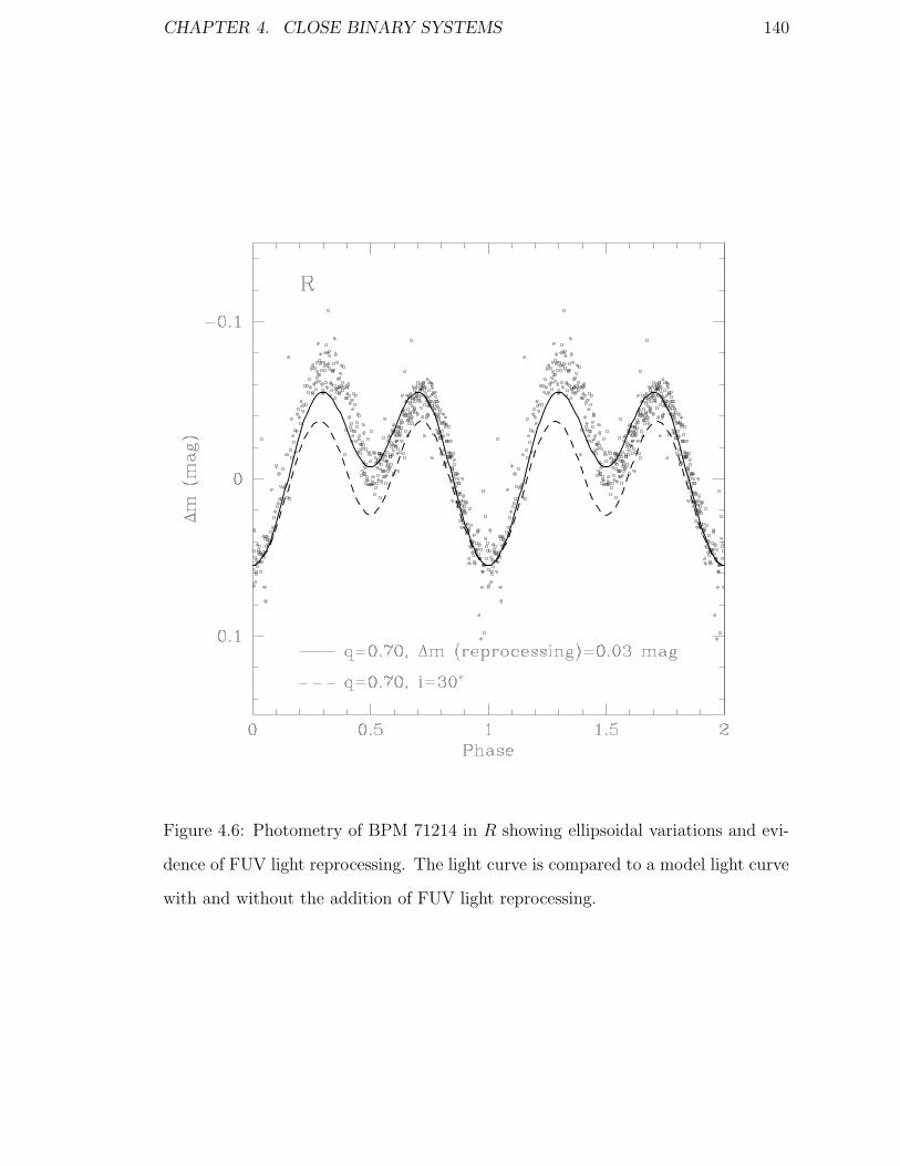
CHAPTER 4. CLOSE BINARY SYSTEMS 140
Figure 4.6: Photometry of BPM 71214 in R showing ellipsoidal variations and evi-
dence of FUV light reprocessing. The light curve is compared to a model light curve
with and without the addition of FUV light reprocessing.

CHAPTER 4. CLOSE BINARY SYSTEMS 141
Table 4.3: Input to the light curve model.
Parameters Input Values
Period 0.201626 days
Inclination 30◦
WD temperature 17200 K
RD temperature 3800 K
WD mass 0.77M�
q (MRD/MWD) 0.50 0.60 0.70
RD mass 0.39M� 0.46M� 0.54M�
RD radius 0.429R� 0.496R� 0.561R�
Separation 1.518R� 1.551R� 1.582R�

CHAPTER 4. CLOSE BINARY SYSTEMS 142
Table 4.4: Properties of the binary BPM 71214
Parameter Measurement Reference
R.A. (epoch = 1997.745) 3 32 43.44 (J2000) 1
Dec. (epoch = 1997.745) −8 55 39.6 (J2000) 1
V, R 13.49, 12.81 2
B 14.2 3
Spectral Type DA + M2.5V 4
WD effective temperature Teff = 17200 ± 1000 K 4
WD surface gravity log g = 8.25 ± 0.10 4
Binary orbital period P = 0.201626 ± 0.000004 d 4
Red dwarf semi-amplitude KdMe = 121.4 ± 1.6 km s−1 4
Systemic velocity 48.7 ± 1.1 km s−1 4
Mass function 0.037 ± 0.002M� 4
Mass of WD 0.77 ± 0.06M� 4
Mass of RD 0.54M� 4
Orbital Separation 1.58R� 4
Inclination 30◦ ± 2◦ 4
Proper motion µ = 0.143′′ yr−1 3
π = 137◦ 3
References- (1) Digitized Sky Survey; (2) GSC II; (3) Luyten (1963);
(4) this work

CHAPTER 4. CLOSE BINARY SYSTEMS 143
observed light curves to model light curves showed that the secondary is indeed very
close to filling its Roche lobe.
BPM 71214 is either a pre-cataclysmic variable, which is just about to begin
mass transfer, or it may be a hibernating nova. The first scenario is less likely, since
the probability of observing a binary just before it begins mass transfer is very small.
Schreiber & Gansicke (2003) calculated the fraction of the post-common envelope
binary lifetime that the system has already passed through for a number of close
binary systems. Using the published results of Kawka et al.(2002), they found that
BPM 71214 has passed through more than 95% of its life as a post-common envelope
binary. The second scenario is more likely since the binary will spend more than
90% of its time in hibernation, where they will appear as close but detached binary
systems.
The first proposal of the hibernation scenario by Shara et al. (1986) and Livio &
Shara (1987) suggested that systems are more likely to go into hibernation after a
nova outburst if there is an increase in separation. This led to the conclusion that for
a given orbital period, systems with a higher mass ratio and shorter orbital periods
are more like to go into hibernation after a nova outburst. BPM 71214 appears to
fit these criteria for a hibernating nova. However, the authors have revised their
calculations (Livio et al., 1991) by incorporating the results of MacDonald (1986) to
find that binary systems with shorter orbital periods will experience a decrease in
orbital separation following a nova outburst rather than an increase in the orbital
separation. They also state that the increase in orbital separation is no longer the
critical mechanism required to reduce the accretion rate in order for the binary
system to go into hibernation following a nova outburst. Prialnik & Kovetz (1995)
calculated evolutionary sequences of nova outbursts through several cycles showing
that the recurrent periods for novae vary from ∼ 100 to 106 years. Therefore, for
some of these systems the white dwarf will have enough time to cool following a nova
outburst and allow the accretion rate to decrease. Following a nova outburst, the

CHAPTER 4. CLOSE BINARY SYSTEMS 144
accretion rate will remain high as a result of the irradiation of the secondary by the
hot white dwarf, however as the white dwarf cools, the accretion rate should decrease,
and possibly allow the system to go into hibernation. Prialnik & Kovetz (1995)
adopted accretion rates that represent the mean of the high- and low-states of mass
transfer, where the high-states occur following a nova outburst changing to low-
states as the white dwarf cools down. The effect of irradiation of the secondary by
the white dwarf on the accretion rate is still uncertain, and whether the accretion
rate can decrease to zero during the lifetime of the nova is also uncertain. However,
the binary parameters of BPM 71214 is suggest that the system should already be a
cataclysmic variable, but no evidence of mass transfer is observed, therefore it may
be a hibernating system.
4.4.2 EUVE J0720-31.7
Orbital Parameters
Table E.5 shows the radial velocity and equivalent width measurements of EUVE
J0720−31.7. Figure 4.7 shows the radial velocities folded on the period with the
periodogram clearly showing the best period. The best orbital period for this system
is:
P = 1.262396 ± 0.000008 d,
with the epoch of inferior conjunction:
T0 = 2451462.277± 0.003 (HJD).
The semi-amplitude of the red dwarf is 98.2±1.2 km s−1 and the systemic veloc-
ity is 31.1±0.7 km s−1. A search for the best period using the equivalent width
measurements resulted in a period of:
P = 1.26243 ± 0.00008 d

CHAPTER 4. CLOSE BINARY SYSTEMS 145
with the epoch of minimum emission:
T0 = 2451461.906± 0.027 (HJD).
This period agrees with the period obtained from radial velocities within the un-
certainties. The EUV illumination model (Thorstensen et al., 1978) predicts that
the maximum emission line strength lags the maximum radial velocity by 0.25 phase
compared to our measured offset of 0.29±0.03. The Hα equivalent widths vary with
a semi-amplitude of 5.24±0.10 A centred about −6.81±0.08 A, which results in an
inclination of 50◦ ± 2◦ using EUV/FUV illumination of the red dwarf model from
Thorstensen et al. (1978). The mass function from these data is 0.124 ± 0.005M�,
which is in agreement with Vennes & Thorstensen (1996).
Spectral Decomposition
The Balmer line spectra from two separate nights of EUVE J0720−31.7 were com-
pared to a grid of models. First the spectra were compared to the grid of models
with the contribution of Hε included and exluded because of the low signal-to-noise
ratio. The core of Hβ (±12 A) was excluded due to the presence of emission. The
average and standard deviation of these measurements provide an effective temper-
ature of Teff = 55550 ± 1360 K and a surface gravity of log g = 7.74 ± 0.07. These
uncertainties constitute a more accurate representation of the errors in temperature
and surface gravity than statistical fitting errors only.
Next, the spectrum of GL 218 (an M1.5 type star) was subtracted until the
TiO bands were no longer observed. The subtracted spectra of EUVE J0720−31.7
were compared with the same grid of model spectra, again including and excluding
Hε, to obtain a mean of Teff = 53900 ± 1770 K and log g = 7.83 ± 0.08. The
effect of subtracting the contribution of the red dwarf is a lower temperature and
a higher gravity. Figure 4.8 shows the Balmer lines EUVE J0720−31.7 from one
of the subtracted spectrum compared to a grid of model spectra, along with the

CHAPTER 4. CLOSE BINARY SYSTEMS 146
Figure 4.7: Radial velocity of the red dwarf in EUVE J0720−31.7 traced by Hα
and folded on the orbital period of 1.262396 d (bottom left), and the period analysis
(top left). Hα equivalent widths phased on the orbital period (1.26243 d) estimated
from these measurements (bottom right), and the period analysis (top right). The
equivalent widths show a phase offset from the radial velocity measurements ∆Φ =
0.29 ± 0.03, close to the predicted offset of 0.25.

CHAPTER 4. CLOSE BINARY SYSTEMS 147
confidence contours for the fit. The mass of the white dwarf is 0.63 ± 0.04M� with
a cooling age of 1.7± 0.1× 10⁶ years, which has been calculated using Wood (1995)
models.
Discussion
Table 4.5 summarizes the properties of the close binary EUVE J0720−31.7. The
contact period for this binary is 0.17 days. The mass of the secondary (M = 0.39M�)
suggests that it is not fully convective and magnetic braking may contribute towards
bringing the binary into contact. Therefore, assuming magnetic braking will be the
major contributor to angular momentum loss, then EUVE J0720−31.7 is expected
to evolve into contact in 8.7 × 10⁹ years. This is enough time for the binary to
evolve into a semi-detached state within a Hubble time which means that it is a
representative progenitor to the currently observed cataclysmic variable stars.
4.4.3 BPM 6502
Orbital Parameters
Table E.6 gives the heliocentric julian dates with the corresponding heliocentric
radial velocities for BPM 6502. The radial velocity measurements were used to
calculate the orbital period of the binary system. The orbital period is:
P = 0.336784 ± 0.000001 d,
and the epoch of inferior conjunction is:
T0 = 2451612.810± 0.001 (HJD).
Figure 4.9 shows the radial velocity measurements of the red dwarf folded on the best
orbital period. The velocity semi-amplitude of the red dwarf 71.7±0.9 km s−1 with
a systemic velocity of 9.2±0.7 km s−1. The white dwarf orbit was determined using
the radial velocity measurements from Hγ, Hδ and Hε absorption lines. The radial
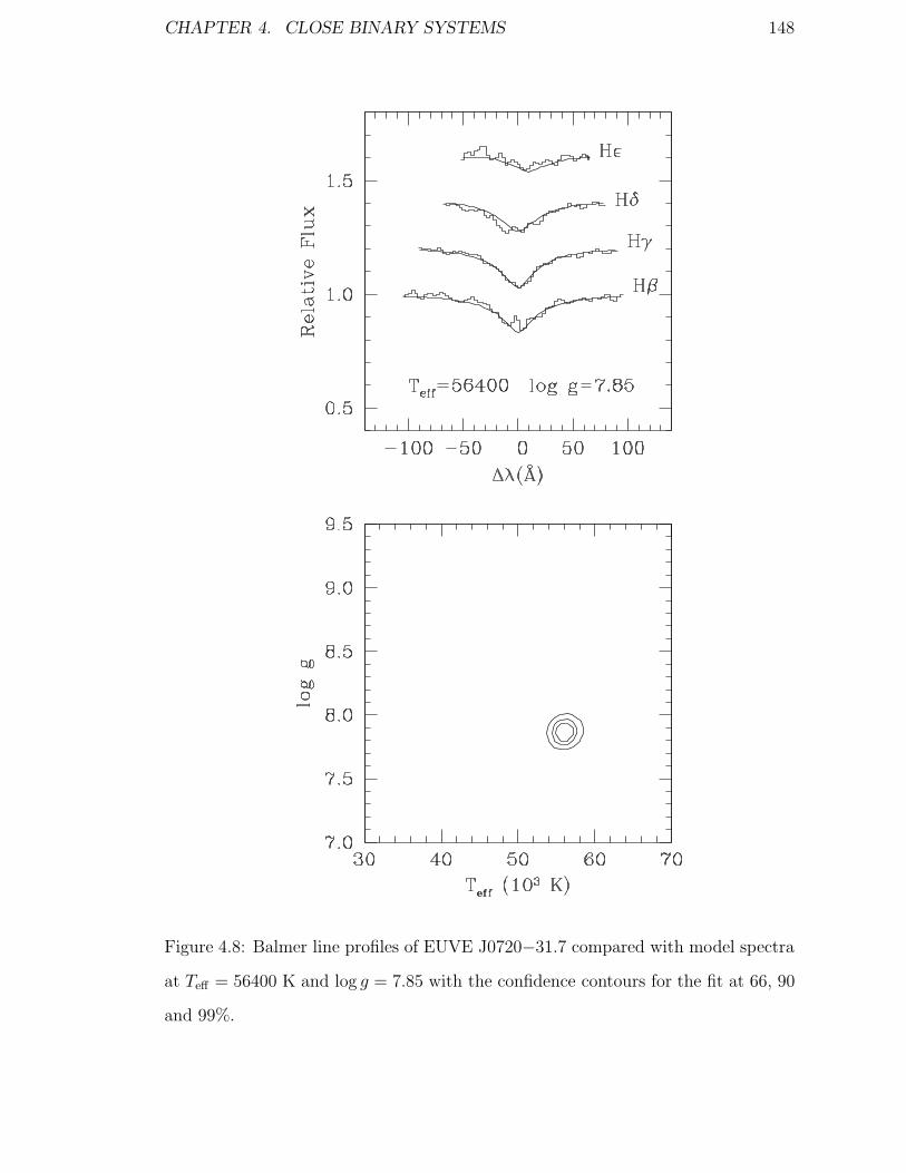
CHAPTER 4. CLOSE BINARY SYSTEMS 148
Figure 4.8: Balmer line profiles of EUVE J0720−31.7 compared with model spectra
at Teff = 56400 K and log g = 7.85 with the confidence contours for the fit at 66, 90
and 99%.

CHAPTER 4. CLOSE BINARY SYSTEMS 149
Table 4.5: Properties of the binary EUVE J0720−31.7
Parameter Measurement Reference
R.A. (epoch = 1995.145) 7 20 47.92 (J2000) 1
Dec. (epoch = 1995.145) −31 47 04.6 (J2000) 1
V 14.82 2
Spectral Type DAO + M1.5V 2,3
WD effective temperature Teff = 53900 ± 1770 K 3
WD surface gravity log g = 7.83 ± 0.08 3
Binary orbital period P = 1.262396 ± 0.000008 d 3
Red dwarf semi-amplitude KdMe = 98.2 ± 1.2 km s−1 3
Systemic velocity 31.1 ± 0.7 km s−1 3
Mass function 0.124 ± 0.005M� 3
Mass of WD 0.63 ± 0.04M� 3
Mass of RD 0.39 ± 0.07M� 4
Orbital Separation 4.96 ± 0.17R� 4
Inclination 50◦ ± 2◦ 3
Proper motion µ = 0.0366′′ yr−1 4
π = 270◦ 4
References- (1) DSS; (2) Vennes & Thorstensen (1994a); (3) this
work; (4) Vennes et al. (1999b)

CHAPTER 4. CLOSE BINARY SYSTEMS 150
velocity measurements for the white dwarf were obtained by first normalizing the
observed spectra and a model template at 20000 K. These spectra were then cross-
correlated using the routine FXCOR in IRAF. The radial velocity measurements of
the white dwarf were phased with the orbital period (P= 0.336784 d) to determine
the velocity semi-amplitude of 25.0 ± 13.0.
Since the red dwarf is illuminated by the hot white dwarf, the Hα emission
traces an orbit inferior to the orbit of the true centre of mass of the secondary.
Correcting for this illumination effect, the velocity semi-amplitude of the red dwarf
is 78.6 ± 7.7 km s−1. For this calculation I have used the Equation 4.4 which is
given in the introduction. The major contributor toward the large uncertainty in
the corrected KRD is the velocity semi-amplitude of the white dwarf. The remainder
of the calculations will assume the corrected velocity semi-amplitude.
The mass function for BPM 6502 is 0.017±0.006 M� and the mass ratio is
0.32 ± 0.22, which results in a red dwarf mass of 0.16 ± 0.12. Using Kepler’s law,
the system inclination can be estimated as:
i = 23◦ ± 3◦.
At this inclination the reprocessing of EUV in the illuminated atmosphere of the
red dwarf should result in Hα equivalent width variations of the order of 40% (i.e.,
≈ sin i) using model A from Thorstensen et al. (1978). These equivalent width mea-
surements were found to be severely affected by blending with the NLTE absorption
core from the white dwarf. To correct for this blending and obtain the true varia-
tions of the Hα emission from the red dwarf, the observed spectra were normalized
to a NLTE model spectrum (TLUSTY, Hubeny & Lanz (1995)) at Teff = 22000 K
and logg = 8.0. The equivalent widths were remeasured. Figure 4.10 shows the
corrected measurements of the equivalent width of Hα emission.

CHAPTER 4. CLOSE BINARY SYSTEMS 151
Figure 4.9: The radial velocity of the red dwarf in BPM 6502 traced by Hα and
folded on the orbital period and best fit (bottom), and the period analysis (top).The
full line shows the 90% confidence level and the dashed line shows the 99% confidence
level of the orbital period.

CHAPTER 4. CLOSE BINARY SYSTEMS 152
Figure 4.10: Hα equivalent width (top) and photometric variations in R (middle)
and I (bottom) of BPM 6502, folded on the orbital period.

CHAPTER 4. CLOSE BINARY SYSTEMS 153
Spectral Decomposition
Figure 4.11 shows the blue and red high-dispersion spectra showing broad Balmer
line absorption from the white dwarf and weak Ca II H and K line emission, as well
as strong Hα emission from the late-type secondary.
Figure 4.12 shows the ultraviolet and optical energy distribution. The ultraviolet
spectra shown are the IUE NEWSIPS spectra LWP 07352 and SWP 27351. The
flux scale was adjusted by +4% and aligned with the Stromgren (uby) photometry.
The Stromgren photometry was obtained by Bessell & Wickramasinghe (1978) and
Wegner (1979), which are in agreement, but the Johnson photometry obtained by
Eggen (1969) appears ∼ 0.3 mag fainter. The distribution was compared to model
spectra at log g = 8.0 and Teff = 20000 and 22000 K, which reveals a best temper-
ature of Teff = 20000 K. This is consistent with the spectrophotometric analysis of
Koester et al. (1979) (Teff = 20311 ± 532 K) and lower than the analysis of Balmer
line profiles of Bragaglia et al. (1995) (Teff = 21380 ± 258 K).
The spectrum of BPM 6502 was compared to a grid of model spectra to obtain a
best fit at Teff = 20640±200 K and log g = 7.73±0.04. Figure 4.13 shows the Balmer
line profiles compared to the best fit model spectrum with the confidence contours
for the fit. Using these values the mass of the white dwarf is 0.49 ± 0.02M� with a
cooling age of 4.0± 0.3× 10⁷ years, which have been calculated using Wood (1995)
models.
Light Curves
Photometric variations with amplitudes 0.0105 and 0.0067 mag in R and I respec-
tively, were observed in BPM 6502. Figure 4.10 shows the I and R photometric
measurements folded over the spectroscopic period and Tables E.11 and E.12 give
the relative photometry measurements of I and R, respectively. The average error
of the photometric measurements is 0.006 mag. The photometric maximum lags
the velocity maximum by 0.25 phase as expected from the illumination effect. The

CHAPTER 4. CLOSE BINARY SYSTEMS 154
Figure 4.11: High-dispersion spectra of BPM 6502 showing weak Ca II H and K
emission and strong Hα emission, which originate from the late-type secondary. The
spectra are compared with a model spectrum at Teff = 22000 K and log g = 8.0.

CHAPTER 4. CLOSE BINARY SYSTEMS 155
Figure 4.12: Ultraviolet (IUE) and optical (Johnson and Stromgren photometry)
spectral distribution of BPM 6502. The distribution is compared with model spectra
at log g = 8.0 and Teff = 20000 and 22000 K.

CHAPTER 4. CLOSE BINARY SYSTEMS 156
Figure 4.13: Balmer line profiles of BPM 6502 compared to model spectra at Teff =
20640K and log g = 7.73 with the confidence contours for the fit at 66, 90 and 99%.
CHAPTER 4. CLOSE BINARY SYSTEMS 157
red dwarf is illuminated by incoming EUV/FUV radiation from the white dwarf,
and the projected area toward the line of sight of the illuminated hemisphere varies
along the orbit, causing the apparent variability.
Discussion
Table 4.6 summarizes the properties of the close binary BPM 6502. The contact
period for this binary is 0.09 ± 0.04 days. The small mass of the secondary implies
that it is fully convective and therefore the orbital angular momentum is assumed
to be lost only by gravitational radiation (1994). BPM 6502 will evolve into contact
in 5.6+3.5−1.7 × 10¹⁰ years, which exceeds a Hubble timescale and is most probably not
a representative progenitor of the currently observed cataclysmic variables.
4.4.4 EC 13471-1258
Orbital Parameters
The Hα emission radial velocity measurements for EC 13471−1258 are given in
Table E.3, with Figure 4.14 showing the radial velocities folded on the best orbital
period of:
P = 0.15074 ± 0.00004 d,
with the epoch of inferior conjunction:
T0 = 2452335.110± 0.006 (HJD).
The semi-amplitude of the red dwarf using Hα emission lines is 241.0 ± 8.1 km s−1
and the systemic velocity is −28.1±5.9 km s−1. Variations in the Hα emission profile
were observed. The most prominent variation is the double peak of the Hα emission
profile, which is observed at quadrature. When the secondary is at conjunction, Hα
emission profile has only one peak. The two peaks may be the result of a varying
temperature distribution on the surface surface of the secondary, since the distortion
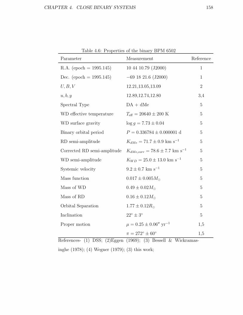
CHAPTER 4. CLOSE BINARY SYSTEMS 158
Table 4.6: Properties of the binary BPM 6502
Parameter Measurement Reference
R.A. (epoch = 1995.145) 10 44 10.79 (J2000) 1
Dec. (epoch = 1995.145) −69 18 21.6 (J2000) 1
U, B, V 12.21,13.05,13.09 2
u, b, y 12.89,12.74,12.80 3,4
Spectral Type DA + dMe 5
WD effective temperature Teff = 20640 ± 200 K 5
WD surface gravity log g = 7.73 ± 0.04 5
Binary orbital period P = 0.336784± 0.000001 d 5
RD semi-amplitude KdMe = 71.7 ± 0.9 km s−1 5
Corrected RD semi-amplitude KdMe,corr = 78.6 ± 7.7 km s−1 5
WD semi-amplitude KWD = 25.0 ± 13.0 km s−1 5
Systemic velocity 9.2 ± 0.7 km s−1 5
Mass function 0.017 ± 0.005M� 5
Mass of WD 0.49 ± 0.02M� 5
Mass of RD 0.16 ± 0.12M� 5
Orbital Separation 1.77 ± 0.12R� 5
Inclination 22◦ ± 3◦ 5
Proper motion µ = 0.25 ± 0.06′′ yr−1 1,5
π = 272◦ ± 60◦ 1,5
References- (1) DSS; (2)Eggen (1969); (3) Bessell & Wickramas-
inghe (1978); (4) Wegner (1979); (3) this work;

CHAPTER 4. CLOSE BINARY SYSTEMS 159
of the secondary is most visible at quadrature, and the strength of the secondary
peaks varies significantly. O’Donoghue et al. (2003) found that the second peak is
tracing an orbit which is on the same side as the centre of mass of the white dwarf,
but is not tracing the expected orbit of the white dwarf. Therefore, O’Donoghue
et al. (2003) concludes that the second peak may originate from mass accretion on
to the white dwarf. Some variation was observed in the stronger component, where
most of the Hα emission is associated with coronal activity (E.W.∼ 5.6A), and only
a small variable proportion is the result of illumination of the red dwarf by the white
dwarf (E.W.= 0.0 − 3.6A)2. There may be some bias in using Hα emission lines in
determining the velocity semi-amplitude of the secondary, meaning that an inferior
orbit to the orbit traced by the true centre of mass of the secondary is favoured.
The radial velocities of absorption lines were obtained by cross-correlating the
absorption features in the wavelength range 6240 to 6540 A against two M-type
spectra (GL 190: M3.5 and GL 250B: M2) using FXCOR in IRAF. Prior to the
cross-correlation, both template spectra were smoothed to the rotational velocity
(140 km s−1) of the secondary. The absorption radial velocity measurements are
given in Table E.4 and the radial velocity measurements that were determined using
GL 250B as a template star is shown in Figure 4.15. The velocities were phased with
the orbital period, and fitted with a sine curve using a least squares fit to obtain:
KRD = 246 ± 14 km s−1 and γ = −19 ± 10 km s−1
when GL 190 was used as a template star, and
KRD = 251 ± 12 km s−1 and γ = −24 ± 8 km s−1
when GL 250B was used as a template star. Both of these measurements are in agree-
ment with the velocity semi-amplitude determined from Hα emission lines within
the 1σ uncertainty. However, these values are significantly different from the veloc-
ity semi-amplitude of 266±6 km s−1 determined by O’Donoghue et al. (2003). The
2Note that the Hα equivalent width flared to 17A on UT 2002 March 8, indicative along with
the noted X-ray emission of strong coronal activity

CHAPTER 4. CLOSE BINARY SYSTEMS 160
Table 4.7: White dwarf radial velocity measurements
HJD (2451410+) V (km s−1)
8.622711 199 ± 36
8.686537 −73 ± 43
8.754354 152 ± 44
reason why the value of O’Donoghue et al. is different from the values obtained in
this work is unknown.
The weighted average of the velocity semi-amplitude measurements from this
work only is 245± 6 km s−1 with a systemic velocity of −25.3± 4.4 km s−1. For the
remaining calculations in this section KRD = 245± 6 km s−1 will be used, however,
when relevant I will also redo the calculation using KRD = 266 ± 6 km s−1 from
O’Donoghue et al. (2003) and do a comparison. The mass function of the white
dwarf is 0.230 ± 0.017M�, but using KRD = 266 ± 6 km s−1 the mass function is
0.294 ± 0.020M�.
The radial velocities of the white dwarf were measured from the STIS spectra
using the absorption lines of C I, N I and Si III. The STIS spectra were obtained
so that they coincided with the binary being observed at quadrature. Three sets of
measurements were obtained that can be used for measuring radial velocities, with
the first set containing 3 exposures, and the other two containing 6 exposures each.
The spectra in each set were combined to increase the signal-to-noise ratio. The
velocities were determined by measuring the shift in wavelength of the lines. Five
lines were used to obtain radial velocity measurements in each spectrum, which
were averaged to obtain a single radial velocity measurement for the spectrum.
Table 4.7 lists the radial velocity measurements for the white dwarf. The radial
velocity measurements were phased with the ephemeris provided by O’Donoghue
et al. (2003) (the ephemeris obtained in this work is not accurate enough for the
phasing of data obtained in 1996). The semi-amplitude of the white dwarf radial

CHAPTER 4. CLOSE BINARY SYSTEMS 161
Figure 4.14: The radial velocity of the red dwarf in EC 13471−1258 traced by
Hα and folded on the orbital period and best fit (bottom), and the period analysis
(top). The full line shows the 90% confidence level and the dashed shows the 99%
confidence level of the orbital period.

CHAPTER 4. CLOSE BINARY SYSTEMS 162
Figure 4.15: Radial velocities traced by absorption features in the wavelength range
6240 to 6540 A for EC 13471−1258 which are folded on the orbital period and
compared to the best sinusoidal fit. The best fit results in a semiamplitude of
251 ± 12 km s−1 and a systemic offset of −24 ± 8 km s−1.

CHAPTER 4. CLOSE BINARY SYSTEMS 163
velocities is 131±17 km s−1 with a mean of 55±16 km s−1. This value is in agreement
with O’Donoghue et al. (2003). The mass ratio from the velocity semi-amplitudes
(KWD/KRD) is 0.54 ± 0.09, implying a secondary mass of 0.42 ± 0.09M�.
Spectral Decomposition
Figure 4.16 shows the spectrum of the red dwarf in EC 13471−1258 which was
observed during the eclipse. The spectra obtained during the eclipse were combined,
and then subtracted from the non-eclipsing spectra obtained shortly before and after
the eclipse to produce a spectrum of the white dwarf. The white dwarf spectrum was
compared to a grid of model spectra to obtain an effective temperature of 14200±500
K and log g = 8.15 ± 0.15. Due to the Balmer line emission, the line cores (±12 A)
were excluded from the fit. The HST data were also compared to the same grid of
models to obtain an effective temperature of 14080± 100 K and log g = 8.26± 0.05.
Therefore, the two measurements are in agreement. Heavy elements are observed
in the FUV spectrum which were not included in the spectral fit. O’Donoghue
et al. (2003) compared the FUV spectrum to model spectra with heavy-elements
for various abundances and obtained a similar temperature and surface gravity.
Figure 4.17 shows the comparisons of the STIS and optical data to the models
with their respective confidence contours. The STIS spectrum shows Lyα satellite
features near 1400 and 1600 A first introduced by Allard & Koester (1992) in the
study of variable ZZ Ceti stars. Figure 4.18 shows the STIS and low-dispersion
optical data compared to a model spectrum at Teff = 14080 K and log g = 8.26, the
red dwarf contribution can be seen at longer wavelengths. The mass of the white
dwarf is 0.77 ± 0.04M� with a cooling age of 3.8 ± 0.3 × 10⁸ years, which has been
calculated using Wood (1995) models.
The Hα emission full width half maximum (FWHM) has been measured in the
high-resolution spectra and the rotational velocity of the red dwarf was calculated.
The FWHM has contributions from sources other than the rotation of the star,

CHAPTER 4. CLOSE BINARY SYSTEMS 164
Figure 4.16: Spectrum of the red dwarf in EC 13471−1258 observed while the white
dwarf was being eclipsed by the red dwarf.

CHAPTER 4. CLOSE BINARY SYSTEMS 165
Figure 4.17: The Balmer lines and Lyman α with the H+2 satellite feature of the white
dwarf in EC 13471−1258 compared to model spectra at 14200 K and log g = 8.15
(top left) 14080 K and log g = 8.15 (top right), with their respective confidence
contours at 66, 90 and 99% (bottom).

CHAPTER 4. CLOSE BINARY SYSTEMS 166
Figure 4.18: STIS and low-dispersion spectra of EC 13471−1258 compared to a
model spectrum at Teff = 14080 K and log g = 8.26.

CHAPTER 4. CLOSE BINARY SYSTEMS 167
which include the intrinsic width of the emission lines, taken as 1.7 A(Houdebine
and Doyle, 1994), a resolution of 1.7 A and the broadening due to the orbital motion
of the secondary. These values were subtracted in quadrature from the measured
FWHM, which resulted in a FWHM of 5.3±1.0 A. The rotational velocity is v sin
i = 140 ± 28 km s−1, and by assuming that the red companion is tidally locked to
the white dwarf, the radius of the red dwarf is 0.42±0.08 R�. Note that this is only
an estimate, and may be influenced by unknown systematic effects.
Light Curves
Figure 4.19 shows the eclipse of the white dwarf in EC 13471−1258 in the B and R
bands, which have been phased with the spectroscopic period. Tables E.9 and E.10
give the relative photometry of EC 13471−1258 in B and R bands, respectively.
The depth of the eclipse is 0.3 mag in R and 1.87 mag in B, which shows that the
red dwarf companion contributed 24% of the luminosity in B and 82% in R. The
red dwarf mass was calculated using the mass function, MWD, orbital period, and
the duration of the eclipse, which is 15.4 ± 1.0 minutes, as inputs into an iterative
code where an initial estimate of the inclination was made. The radius of the red
dwarf was assumed to be the Roche lobe radius, which was checked against the
radius obtained from the FWHM of Hα emission. The relation used to calculate the
inclination in the code was:
cos2 i =
(RRD
a
)2 − sin2 (π∆φ)
cos2 (π∆φ)(4.6)
where ∆φ is the phase width of the eclipse (Horne et al., 1982). Therefore, the
inclination of the system is:
i = 73.8 ± 1.5◦.
The mass of the red dwarf companion determined from the mass function is 0.55 ±0.11M�, which results in a mass ratio of 0.72± 0.10 and a separation of the binary
CHAPTER 4. CLOSE BINARY SYSTEMS 168
of 1.31 ± 0.05R�. This appears to differ from the value obtained purely from the
velocity semi-amplitudes, however they are consistent within the uncertainties. Since
the mass ratio and hence secondary mass strongly depend on the red dwarf velocity
semi-amplitude, then the difference in the two values of the secondary mass must be
a result of KRD. A more consistent result between the two methods of determining
the mass of the secondary would be achieved if the red dwarf velocity semi-amplitude
is ∼ 10% larger, which is approximately what O’Donoghue et al. (2003) obtained.
Using the KRD of O’Donoghue et al. rather than the KRD obtained in this study,
the mass of the secondary would be 0.41 ± 0.09M� with a separation of the binary
of 1.26 ± 0.04. The inclination would be 75.7 ± 1.9◦ which is consistent with the
inclination determined with the lower mass function.
The radius of the Roche lobe is 0.46 ± 0.02R�, which is in agreement with the
secondary radius measured from the FWHM of the Hα emission. This implies that
the red dwarf is very close to filling its Roche lobe, since there is no evidence of on-
going mass transfer. At a first glance the radius and mass of the red dwarf appear
discrepant. Using mass-radius relations for M-dwarfs, the expected radius for an
M-dwarf with a mass of 0.55M� is 0.57R�, which contradicts the measured value,
however comparison to other M-dwarfs of similar mass shows that the radius is not
unreasonably too small, and that it is within the scatter of values (Caillault and
Patterson, 1990; Clemens et al., 1998). A lower secondary mass (0.42M�) is more
consistent with the observed red dwarf radius. Therefore the mass of the secondary
is most probably somewhere between the two values (0.42 − 0.55M�).
The light curve shows ellipsoidal variations from the distorted red dwarf. The
amplitudes of the variations are 0.194 and 0.050 in R and B, respectively. The true
amplitude of the ellipsoidal variation corrected for white dwarf continuum dilution
estimated from the eclipse is ∆R = 0.24±0.02 and ∆B = 0.21±0.09. This amplitude
can be used to determine the inclination of the system, but it is also sensitive to the
value used for gravitational darkening (Warner, 1995). Adopting i = 73.8◦ and using

CHAPTER 4. CLOSE BINARY SYSTEMS 169
Figure 4.19: Photometry of EC 13471−1258 in R and B showing the ellipsoidal
variations and the eclipse. The depth of the eclipse is 0.3 magnitudes in R and 1.85
magnitudes in B with a duration of 15.4 minutes, and the semi-amplitudes of the
ellipsoidal variations are 0.097 and 0.025 magnitudes in R and B, respectively. The
light curves are compared to a model light curves (solid black line). There is no
evidence of illumination of the red dwarf by the white dwarf.
CHAPTER 4. CLOSE BINARY SYSTEMS 170
the gravitational darkening coefficient at 7000 A, ug = 1.29 (Russell, 1945; Kopal,
1959), the amplitude would be 0.28±0.04, compared with 0.17±0.03 for ug = 0.412
(Lucy, 1967) and 0.15 ± 0.02 for ug = 0.257 (Claret, 2000). A blackbody spectrum
was assumed in these calculations, which means that it may also be responsible for
the disagreement between the predicted and observed amplitudes.
The light-curve for EC 13471−1258 was compared to model light curves which
were calculated using the WD code (Wilson, 1979; Wilson, 1990). As for BPM
71214, a detached system (MODE = 2) is assumed. Black-body source spectra
are assumed with no spots present on the surface of the primary or the secondary,
and reflection was allowed with albedos = 1. The white dwarf mass was fixed
at 0.77M�, the inclination at 73.5◦ and the white dwarf temperature at 14085 K.
The temperature of the red dwarf was varied until the depth of the eclipse was
satisfied. The radius of the red dwarf was varied until the amplitude of the ellipsoidal
variations was satisfied.
The mass of the red dwarf was fixed at 0.55M�. Model light curves were also
computed using a secondary mass of 0.42M�. I noted that when the mass of the
secondary is decreased the separation must also decrease, and, therefore, the mass of
the secondary has little effect on the resulting light curves, unless strict mass-radius
relations are kept.
First, the R light curve was fitted, and TRD = 2790 K and RRD = 0.44R�
provided the best fit. I then adopted these parameters for the B light curve, but
the red dwarf temperature had to be increased to 2980 K. Since the spectrum of the
M-dwarf cannot be well represented with a blackbody, the red dwarf temperature of
2900±150 K is only an estimate. O’Donoghue et al. (2003) adopted a temperature of
3100±75 K using colours, and therefore the temperature of 2900 K is an acceptable
estimate.
CHAPTER 4. CLOSE BINARY SYSTEMS 171
Discussion
Table 4.8 summarizes the properties of the close binary EC 13471−1258. The con-
tact period for this binary system is 0.152 d, therefore the observed orbital period
of EC 13471−1258 is slightly smaller than the predicted contact orbital period,
implying that the binary should already be in contact. The ellipsoidal variations
observed in the B and R bands showed that the secondary is filling its Roche lobe.
High-resolution spectroscopy of Hα revealed that the emission line is made up of
two components. The dominant component originates from the active secondary
star and second component which only appears at quadrature could be the result
of a varying temperature structure of the secondary. O’Donoghue et al. (2003) also
observed two peaks in the Hα emission lines, and suggested that the second emission
peak originates from the Roche lobe of the white dwarf implying that there may be
some very weak mass transfer.
As in BPM 71214, EC 13471−1258 is either a pre-cataclysmic variable which
is just about to come into contact, or it may be a hibernating nova. The first
scenario is very unlikely for the same reason given for BPM 71214. Schreiber &
Gansicke (2003) found that EC 13471−1258 has passed through more than 99% of
its life as a post-common envelope binary. Therefore, the hibernation scenario is
more likely.
4.5 Summary
Four close binary systems were studied, for which orbital and atmospheric param-
eters were obtained. Two of these systems, BPM 6502 and EUVE J0720−31.7 are
post-common envelope binary systems. The orbital parameters of EUVE J0720−31.7
suggest that it is likely to come into contact within a Hubble time and is representa-
tive of the population of progenitors from which the currently observed cataclysmic
variables have evolved. However, the properties of BPM 6502 suggest that the bi-

CHAPTER 4. CLOSE BINARY SYSTEMS 172
Table 4.8: Properties of the binary EC 13471−1258
Parameter Measurement Reference
R.A. (epoch = 1995.145) 13 49 51.95 (J2000) 1
Dec. (epoch = 1995.145) −13 13 37.5 (J2000) 1
V a 14.7 2
Spectral Type DA + M2-4 3
WD effective temperature Teff = 14085 ± 100 K 3
WD surface gravity log g = 8.25 ± 0.05 3
Binary orbital period P = 0.15074 ± 0.00004 d 3
Red dwarf semi-amplitude KdMe = 245 ± 6 km s−1 3
KdMe = 266 ± 6 km s−1 4
White dwarf semi-amplitude KDA = 131 ± 17 km s−1 3
Systemic velocity −25.3 ± 4.4 km s−1 3
Mass function 0.230 ± 0.017M� 3
0.294 ± 0.020M�a 3
Mass of WD 0.77 ± 0.04M� 3
Mass of RD 0.55 ± 0.11M� 3
0.41 ± 0.09Ma� 3
Orbital Separation 1.31 ± 0.05R� 3
1.26 ± 0.04Ra� 3
Inclination 73.8◦ ± 1.5◦ 3
References- (1) DSS; (2) Kilkenny et al. (1997); (3) this work; (4)
O’Donoghue et al. (2003)
aUsing KdMe of O’Donoghue et al. (2003)

CHAPTER 4. CLOSE BINARY SYSTEMS 173
nary will not come into contact within a Hubble time. Other post-common envelope
binaries that are likely to come into contact within a Hubble time and are within
100 pc of the Sun are V471 Tau, HR Cam, MS Peg and EG UMa (Schreiber and
Gansicke, 2003). Moreover, (Schmidt et al., 2003) estimate that six systems, two
of them within 50 pc of the Sun (EG UMa, V471 Tau), will initiate mass transfer
within a billion years.
The other two binary systems, BPM 71214 and EC 13471−1258, have orbital
parameters that suggest that these systems should already be in contact and are the
closest to interaction. Ellipsoidal variations were observed in both of these systems
implying that the secondary stars in these systems are filling their Roche lobe.
No evidence of mass transfer that would categorize these systems as cataclysmic
variables was found. Therefore, these systems are most likely hibernating novae.
All of these binaries are relatively nearby with EUVE J0720−31.7 being the
furthest away at a distance of ∼ 150 pc and BPM 6502 being the closest binary at
∼ 29 pc. Therefore, hibernating nova candidates and pre-cataclysmic variables do
inhabit the Solar neighbourhood.

Chapter 5
Conclusion
5.1 Main Results
In this work, I have carried out a study of white dwarfs in the Solar neighbourhood.
The properties of white dwarfs were studied, which included their temperature, mass,
magnetic field strength, binarity and kinematics. Since many of the white dwarfs
that were studied were cool, the model atmosphere code was modified to include
convective energy transfer so that an analysis of cool high-density atmospheres was
possible. Model atmospheres were calculated for varying white dwarf surface gravi-
ties and for temperatures ranging from 4500 K to 84000 K. These model atmospheres
were then used to compute synthetic spectra for white dwarfs with a hydrogen-rich
atmosphere. The code used to calculate synthetic spectra was modified to include
the effect of resonance broadening in the hydrogen lines due to collision with neutral
particles.
The magnetic properties of the white dwarf population was studied, in particular
a spectropolarimetric survey of white dwarfs in the southern hemisphere was con-
ducted at the 74 inch telescope at MSO. This survey complemented a similar survey
conducted by Schmidt & Smith (1995). No new magnetic white dwarfs were found
in the survey of white dwarfs in the southern hemisphere, however this survey along
174

CHAPTER 5. CONCLUSION 175
with the northern survey has helped constrain the incidence of magnetism among
white dwarfs. I reviewed the list of known white dwarfs in the Solar neighbourhood
and found that 17% of these white dwarfs are magnetic, which is significantly higher
than other independent estimates.
The origin of magnetism in white dwarfs was investigated as part of this thesis.
The assumption that Ap and Bp stars are progenitors to magnetic white dwarfs was
tested. The observed space density of magnetic white dwarfs was compared to the
predicted space density of Ap and Bp remnants. I found that:
• Ap and Bp stars can only explain white dwarfs with magnetic fields greater
than 100 MG.
• There are not enough Ap and Bp stars to explain the 17% incidence of mag-
netism in white dwarfs.
• Normal main-sequence stars with weak magnetic fields may be required to
explain the large number of white dwarfs with low magnetic fields.
The study assumed that no magnetic flux is lost during the final stages of evolution,
which may not the best assumption, since some magnetic flux may be carried away
during the mass loss period. The average mass of magnetic white dwarfs is higher
than predicted by the initial-to-final mass relation for normal white dwarfs implying
that magnetic fields may inhibit mass loss.
The properties of white dwarfs in the Solar neighbourhood were further explored
by re-observing five stars from a list of local white dwarfs (Holberg et al., 2002)
and twelve new white dwarfs from the NLTT catalogue (Luyten, 1979; Salim and
Gould, 2003). As a result three stars from the list of local white dwarfs were found
not to be white dwarfs, but rather F-type stars. Observations of NLTT white dwarf
candidates resulted in the discovery of three white dwarfs within 20 pc of the Sun,
and another six with distances between 20 and 30 pc. The nearby white dwarfs that
were found were mostly cool, and the three objects that were within 20 pc of the
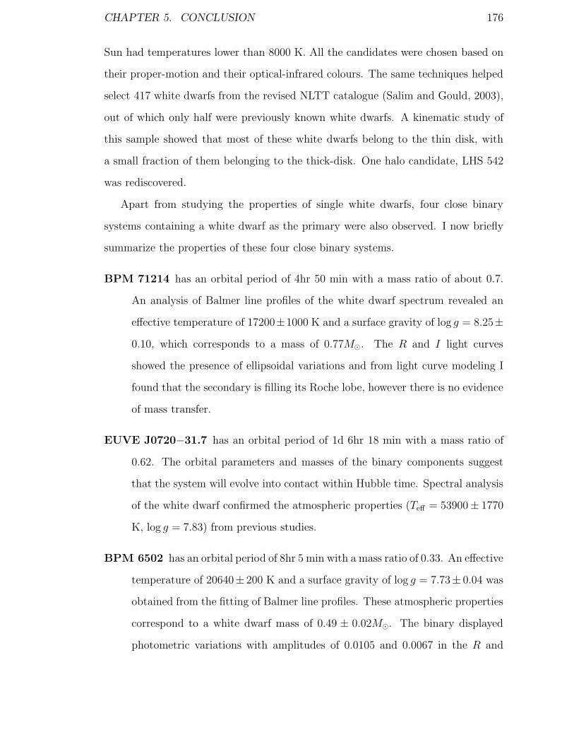
CHAPTER 5. CONCLUSION 176
Sun had temperatures lower than 8000 K. All the candidates were chosen based on
their proper-motion and their optical-infrared colours. The same techniques helped
select 417 white dwarfs from the revised NLTT catalogue (Salim and Gould, 2003),
out of which only half were previously known white dwarfs. A kinematic study of
this sample showed that most of these white dwarfs belong to the thin disk, with
a small fraction of them belonging to the thick-disk. One halo candidate, LHS 542
was rediscovered.
Apart from studying the properties of single white dwarfs, four close binary
systems containing a white dwarf as the primary were also observed. I now briefly
summarize the properties of these four close binary systems.
BPM 71214 has an orbital period of 4hr 50 min with a mass ratio of about 0.7.
An analysis of Balmer line profiles of the white dwarf spectrum revealed an
effective temperature of 17200±1000 K and a surface gravity of log g = 8.25±0.10, which corresponds to a mass of 0.77M�. The R and I light curves
showed the presence of ellipsoidal variations and from light curve modeling I
found that the secondary is filling its Roche lobe, however there is no evidence
of mass transfer.
EUVE J0720−31.7 has an orbital period of 1d 6hr 18 min with a mass ratio of
0.62. The orbital parameters and masses of the binary components suggest
that the system will evolve into contact within Hubble time. Spectral analysis
of the white dwarf confirmed the atmospheric properties (Teff = 53900± 1770
K, log g = 7.83) from previous studies.
BPM 6502 has an orbital period of 8hr 5 min with a mass ratio of 0.33. An effective
temperature of 20640± 200 K and a surface gravity of log g = 7.73± 0.04 was
obtained from the fitting of Balmer line profiles. These atmospheric properties
correspond to a white dwarf mass of 0.49 ± 0.02M�. The binary displayed
photometric variations with amplitudes of 0.0105 and 0.0067 in the R and

CHAPTER 5. CONCLUSION 177
I bands, respectively, which are the result of the cool secondary star being
illuminated by the hot white dwarf. The orbital parameters and the masses
of the binary components suggest that the system will not evolve into contact
within a Hubble time. However, the mass of the secondary is very uncertain,
and a larger mass for the secondary will allow the system to evolve into a
cataclysmic variable within a Hubble time.
EC 13471−1258 has an orbital period of 3hr 37 min. An effective temperature of
14085±100 and a surface gravity of log g = 8.25±0.05 was obtained from the
spectral analysis of the white dwarf’s Balmer line profiles. This system is an
eclipsing binary and photometry in the B and R bands also display ellipsoidal
variations. Light curve modeling of these variations shows that the secondary
is filling its Roche lobe, however there is no evidence of mass transfer via the
centre of mass of the binary (the inner Lagrangian point). The mass of the
secondary is 0.41 − 0.55M� and is somewhat uncertain.
The properties of BPM 71214 and EC 13471−1258 suggest that these systems are
hibernating novae. The theory of hibernating novae was first introduced to explain
the deficiency in the observed rate of novae in our Galaxy. The general hibernating
nova scenario is that a binary will evolve into a nova after non-conservative mass
transfer leads to a build up of mass on the white dwarf which leads to a TNR.
Following the TNR mass ejection continues for a few weeks to months until most of
the mass is ejected. Once the white dwarf stops ejecting mass, mass transfer from
the red dwarf onto the white dwarf continues. The illumination of the red dwarf by
the hot white dwarf keeps the mass transfer high, but as the white dwarf cools, the
radius of the red dwarf decreases until it underfills its Roche lobe, causing the mass
transfer to cease. The binary can remain in this state for about 103 − 106 years.
The binary will again initiate mass transfer when the binary comes into contact via
the loss of angular momentum due to gravitational radiation or magnetic braking.
Shara et al. (1986) predicted that the closest such system should be only ∼ 20 pc

CHAPTER 5. CONCLUSION 178
away, and in this thesis two hibernating nova candidates have been identified. The
estimated distance for BPM 71214 is 68 pc and for EC 13471−1258 is 55 pc.
BPM 71214 and EC 13471−1258 are the only known close binary systems that
are very close to interaction. However, there are other binary systems, like EUVE
J0720−31.7 that will come into contact within a Hubble time, and are representa-
tive of the population of progenitors from which the currently observed cataclysmic
variables have evolved.
5.2 Future Work
The model atmosphere and spectral synthesis codes presented in this thesis can be
used to calculate hydrogen rich white dwarf spectra with temperatures as low as
4500 K. However, the code will need to be modified to include helium in the atmo-
sphere. Moreover, the contribution of molecular hydrogen needs to be considered
in cool white dwarfs. The effect of collision induced absorption (CIA) by molecular
hydrogen (H2) with H2, H and He if helium is present in the atmosphere becomes
important for white dwarf with effective temperatures below 6000 K and in the
infrared region of the spectrum (Bergeron et al., 1995a). Therefore, the model at-
mosphere code and the spectral synthesis code will require additional modifications
so that a larger variety of white dwarfs can be studied.
The spectropolarimetric survey of white dwarfs has contributed toward con-
straining the incidence of magnetism within the Solar neighbourhood. However,
only about 40% of the white dwarfs within 20 pc have been observed spectropo-
larimetrically. The polarization properties of the remaining 60% of the local white
dwarfs should be measured. This will help in obtaining an accurate magnetic field
distribution of white dwarfs in the Solar neighbourhood. By improving our knowl-
edge of the incidence of magnetism in white dwarfs, and of their mass and tempera-
ture distributions, reliable estimates of the formation rate and better understanding

CHAPTER 5. CONCLUSION 179
of the origin and evolution of magnetic white dwarfs would be possible.
I will expand further my investigation of white dwarfs in the Solar neighbour-
hood by confirming the identification of 200 NLTT white dwarfs candidates not yet
observed spectroscopically, and obtain measurements of their temperatures and sur-
face gravities. Moreover, accurate radial velocity measurements should be obtained
for the total sample of 417 colour-selected white dwarfs to improve the population
kinematics. The membership of these white dwarfs to the thin disk, thick disk or
halo should be re-investigated.
Following-up on my work on close binary systems, one key property that requires
confirmation is the mass of the secondary stars. This can be achieved by obtaining
accurate white dwarf radial velocities and calculating the mass ratio of each sys-
tem. White dwarf radial velocities were already obtained for EUVE J0720−31.7 by
Vennes, Thorstensen & Polomski (1999b) and EC 13471−1258 by O’Donoghue et
al. (2003) using heavy element absorption lines. A confirmation of the secondary
mass is still required for BPM 6502 and BPM 71214, and this can be achieved by
measuring metal absorption lines in FUV/EUV spectra. Both BPM 6502 and BPM
71214 are expected to show the presence of metal lines in the spectra, a result of
accretion from the secondary companions.

Appendix A
Known Magnetic White Dwarfs
Table A.1 lists the known magnetic white dwarfs. The first column gives the WD
number, the second column gives an alternate name. In column 3 the composition of
the white dwarf is given, in column 4 the polar magnetic field strength is given unless
otherwise stated, the effective temperature and mass of the white dwarf are given
in columns 5 and 6. The rotational period is given in column 7 and the references
are listed in the final column.
Table A.2 lists the white dwarfs that have once been classified as magnetic, but
where more recent research found them to be non-magnetic white dwarfs. The WD
number and an alternate name are given in columns 1 and 2. Column 3 gives the
spectral type with the effective temperature and mass of the white dwarf (if the
authors assumed log g = 8 in their calculations then this is stated) in columns 4 and
5. The final column provides the references.
180

APPENDIX A. KNOWN MAGNETIC WHITE DWARFS 181
Tab
leA
.1:
Mag
net
icW
hit
eD
war
fsW
DO
ther
Nam
esC
omp.
Bp
(MG
)T
eff(K
)M
(M�)
Prot
Ref
eren
ces
0003−1
03SD
SSJ0
0055
5.91−1
0021
3.4
DQ
?1
0009
+50
1LH
S10
38H
�0.
265
40±
150
0.74
±0.
042−
20hr
2,3
0011−1
34LH
S10
44H
16.7
±0.
660
10±
120
0.71
±0.
074,
300
15+
004
SDSS
J001
742.
44+
0041
37.4
He
8.3
1500
01
0040
+00
0SD
SSJ0
0424
8.19
+00
1955
.3a
H14
1100
01
0041−1
02Fe
ige
7H
/He
3520
000
log
g=
(8.0
)13
1.60
6m
in5
0140
+13
0SD
SSJ0
1424
5.37
+13
1546
.4H
e4
1500
01
0155
+00
3SD
SSJ0
1574
8.15
+00
3315
.1M
g,N
a,C
a3.
71
0159−0
32M
WD
0159−0
32H
626
000
log
g=
(8.0
)6
0208
+00
2SD
SSJ0
2111
6.34
+00
3128
.5H
490
9000
:1
0236−2
69H
E02
36−2
656b
He
?60
00−
7000
902
53+
508
KP
D02
53+
5052
H13
−14
1500
0lo
gg
=(8
.0)
702
57+
080
LH
S50
64H
∼0.
166
80±
150
0.57
±0.
093
0301−0
06SD
SSJ0
3040
7.40−0
0254
1.7
H10
.815
000
803
07−4
28M
WD
0307−4
28H
1025
000
log
g=
(8.0
)6
0325−8
57E
UV
EJ0
317−
855
H18
5−
450
3300
01.
3572
5s
803
29−0
05K
UV
0329
2−00
35H
12.1
2650
09
Con
tinu
eson
next
page
aun
reso
lved
doub
lede
gene
rate
bPol
ariz
atio
nha
sbe
enob
serv
edby
Schm
idt
etal
.20
01

APPENDIX A. KNOWN MAGNETIC WHITE DWARFS 182
Tab
leA
.1–
cont
inue
dfr
ompr
evio
uspa
geW
DO
ther
Nam
esC
omp.
Bp
(MG
)T
eff(K
)M
(M�)
Prot
Ref
eren
ces
0330−0
00H
E03
30−0
002a
He
?60
00−
7000
1003
40−0
68SD
SSJ0
3430
8.18−0
6412
7.3
H45
1300
0:1
0342
+00
4SD
SSJ0
3451
1.11
+00
3444
.3H
1.5
8000
904
13−0
7740
Eri
BH
0.00
23±
0.00
0716
490±
840.
497±
0.00
511
,12
0503−1
74LH
S17
34H
7.3±
0.2
5300
±12
00.
37±
0.07
4,3
0548−0
01G
99−3
7C
2/C
H∼
1064
00±
140
0.78
±0,
034.
117
hr13
,3,1
405
53+
053
G99−4
7H
20±
357
90±
110
0.71
±0.
030.
97hr
15,3
,14
0616−6
49E
UV
EJ0
616−
649
H14
.850
000
log
g=
(8.0
)16
0637
+47
7G
D77
H1.
2±
0.2
1487
0±
120
0.69
17,1
807
28+
642
G23
4−4
H0.
0396
±0.
0116
a45
00±
500
1907
55+
358
SDSS
J075
819.
57+
3544
43.7
H27
2200
01
0756
+43
7G
111−
49H
220
8500
±50
020
,19
0804
+39
7SD
SSJ0
8074
3.33
+39
3829
.2H
4913
000
108
16+
376
GD
90H
914
000
log
g=
(8.0
)21
,19
0821−2
52E
UV
EJ0
823−
254
H2.
8−
3.5
4320
0±
1000
1.20
±0.
0422
0837
+19
9E
G61
H∼
317
100±
350
0.81
7±
0.03
223
0839
+02
6SD
SSJ0
8415
5.74
+02
2350
.6H
670
001
0843
+48
8SD
SSJ0
8471
6.21
+48
4220
.4b
H∼
319
000
108
53+
163
LB
8827
H/H
e0.
75−
1.0
2400
0lo
gg
=(8
.0)
2408
55+
416
SDSS
J085
830.
85+
4126
35.1
H2
7000
:1
Con
tinu
eson
next
page
aLon
gitu
dina
lfiel
d,B
ebun
reso
lved
doub
lede
gene
rate

APPENDIX A. KNOWN MAGNETIC WHITE DWARFS 183
Tab
leA
.1–
cont
inue
dfr
ompr
evio
uspa
geW
DO
ther
Nam
esC
omp.
Bp
(MG
)T
eff(K
)M
(M�)
Prot
Ref
eren
ces
0912
+53
6G
195−
19H
e∼
100
7160
±19
00.
75±
0.02
1.33
01±
0004
d13
,3,2
509
22+
014
SDSS
J092
527.
47+
0113
28.7
H2.
210
000
109
30+
010
SDSS
J093
313.
14+
0051
35.4
He
(C2H
)?1
0945
+24
6LB
1114
6H
670
1600
0±
2000
0.90
+0.1
0−0
.14
26,2
709
57+
022
SDSS
J100
005.
67+
0158
59.2
H20
9000
110
08+
290
LH
S22
29H
e(C
2H
)∼
100
4600
2810
13+
044
SDSS
J101
618.
37+
0409
20.6
H7.
510
000
110
15+
014
PG
1015
+01
4H
120±
1014
000
log
g=
(8.0
)98
,747
34±
0.00
007
min
29,3
0,31
1017
+36
7G
D11
6H
65±
516
000
3210
26+
117
LH
S22
73H
1871
60±
170
(0.5
9)33
1031
+23
4P
G10
31+
234
H∼
200−
1000
∼15
000
3.39
97±
0.00
03hr
34,3
5,36
1033
+65
6SD
SSJ1
0365
5.38
+65
2252
.0D
Q?
110
36−2
04LP
790−
29H
e50
7800
log
g=
(8.0
)24
−28
d37
,38
1043−0
50H
E10
43−0
502
He
∼82
0∼
1500
039
,10
1045−0
91H
E10
45−0
908
H∼
9−
3192
00±
500
log
g=
(8.0
)∼
2−
4hr
40,1
010
50+
598
SDSS
J105
404.
38+
5933
33.3
H17
9500
110
53+
656
SDSS
J105
628.
49+
6523
13.5
H28
1650
01
1107
+60
2SD
SSJ1
1101
0.50
+60
0141
.4H
6.5
3000
01
1111
+02
0SD
SSJ1
1134
1.33
+01
4641
.7H
e?
111
26−0
08SD
SSJ1
1285
2.88−0
1054
0.8
H3
1100
01
1131
+52
1SD
SSJ1
1335
7.66
+51
5204
.8H
7.5
2200
01
1136−0
15LB
QS
1136−0
132
H24
±1
1050
041
Con
tinu
eson
next
page

APPENDIX A. KNOWN MAGNETIC WHITE DWARFS 184
Tab
leA
.1–
cont
inue
dfr
ompr
evio
uspa
geW
DO
ther
Nam
esC
omp.
Bp
(MG
)T
eff(K
)M
(M�)
Prot
Ref
eren
ces
1137
+61
4SD
SSJ1
1400
6.37
+61
1008
.2H
5813
500
111
51+
015
SDSS
J115
418.
14+
0117
11.4
H32
2700
0:1
1156
+61
9SD
SSJ1
1591
7.39
+61
3914
.3H
15.5
2300
01
1209
+01
8SD
SSJ1
2120
9.31
+01
3627
.7H
1310
000
112
11−1
71H
E12
11−1
707
He
50∼
1200
0∼
2hr
1012
12−0
22SD
SSJ1
2145
6.39−0
2340
2.8
DZ
1.9
112
14−0
01SD
SSJ1
2163
5.37−0
0265
6.2
H63
2000
09
1219
+00
5SD
SSJ1
2220
9.44
+00
1534
.0H
1214
000
112
20+
234
PG
1220
+23
4H
∼3
2654
00.
8131
1246−0
22SD
SSJ1
2485
1.31−0
2292
4.7
H7
1350
01
1254
+34
5H
S12
54+
3440
H9.
5±
0.5
1500
0±
4000
4213
09+
853
G25
6−7
H4.
9±
0.5
∼56
000
2013
12+
098
PG
1312
+09
8H
10∼
2000
05.
4283
9±
0.00
001
hr31
,19
1330
+01
5G
62−4
6aH
7.36
±0.
1160
40−
6110
0.14
−0.
6743
1331
+00
5SD
SSJ1
3335
9.86
+00
1654
.8H
e(C
2H
)?
113
32+
643
SDSS
J133
340.
34+
6406
27.4
H13
1350
01
1339
+65
9SD
SSJ1
3404
3.10
+65
4349
.2H
315
000
113
49+
545
SBS
1349
+54
34H
760
∼11
000
4413
50−0
90LP
907−
037
H�
0.3
9500
±10
01.
08±
0.15
214
40+
753
EU
VE
J143
9+75
0bH
14−
1620
000−
5000
00.
88−
1.19
4514
44+
592
SDSS
J144
614.
00+
5902
16.7
H7
1250
01
Con
tinu
eson
next
page
aun
reso
lved
doub
lede
gene
rate
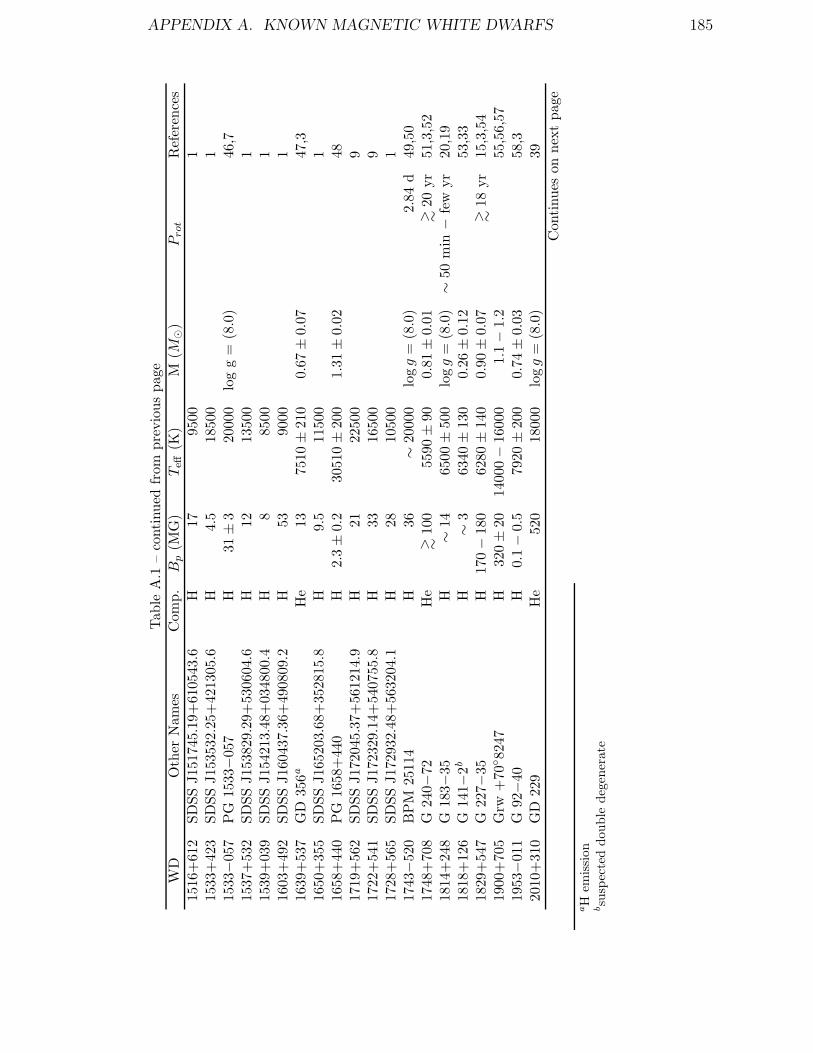
APPENDIX A. KNOWN MAGNETIC WHITE DWARFS 185
Tab
leA
.1–
cont
inue
dfr
ompr
evio
uspa
geW
DO
ther
Nam
esC
omp.
Bp
(MG
)T
eff(K
)M
(M�)
Prot
Ref
eren
ces
1516
+61
2SD
SSJ1
5174
5.19
+61
0543
.6H
1795
001
1533
+42
3SD
SSJ1
5353
2.25
+42
1305
.6H
4.5
1850
01
1533−0
57P
G15
33−0
57H
31±
320
000
log
g=
(8.0
)46
,715
37+
532
SDSS
J153
829.
29+
5306
04.6
H12
1350
01
1539
+03
9SD
SSJ1
5421
3.48
+03
4800
.4H
885
001
1603
+49
2SD
SSJ1
6043
7.36
+49
0809
.2H
5390
001
1639
+53
7G
D35
6aH
e13
7510
±21
00.
67±
0.07
47,3
1650
+35
5SD
SSJ1
6520
3.68
+35
2815
.8H
9.5
1150
01
1658
+44
0P
G16
58+
440
H2.
3±
0.2
3051
0±
200
1.31
±0.
0248
1719
+56
2SD
SSJ1
7204
5.37
+56
1214
.9H
2122
500
917
22+
541
SDSS
J172
329.
14+
5407
55.8
H33
1650
09
1728
+56
5SD
SSJ1
7293
2.48
+56
3204
.1H
2810
500
117
43−5
20B
PM
2511
4H
36∼
2000
0lo
gg
=(8
.0)
2.84
d49
,50
1748
+70
8G
240−
72H
e�
100
5590
±90
0.81
±0.
01�
20yr
51,3
,52
1814
+24
8G
183−
35H
∼14
6500
±50
0lo
gg
=(8
.0)
∼50
min
−fe
wyr
20,1
918
18+
126
G14
1−2b
H∼
363
40±
130
0.26
±0.
1253
,33
1829
+54
7G
227−
35H
170−
180
6280
±14
00.
90±
0.07
�18
yr15
,3,5
419
00+
705
Grw
+70
◦ 824
7H
320±
2014
000−
1600
01.
1−
1.2
55,5
6,57
1953−0
11G
92−4
0H
0.1−
0.5
7920
±20
00.
74±
0.03
58,3
2010
+31
0G
D22
9H
e52
018
000
log
g=
(8.0
)39
Con
tinu
eson
next
page
aH
emis
sion
bsu
spec
ted
doub
lede
gene
rate

APPENDIX A. KNOWN MAGNETIC WHITE DWARFS 186
Tab
leA
.1–
cont
inue
dfr
ompr
evio
uspa
geW
DO
ther
Nam
esC
omp.
Bp
(MG
)T
eff(K
)M
(M�)
Prot
Ref
eren
ces
2043−0
73SD
SSJ2
0462
6.15−0
7103
7.0
H2
8000
120
49−0
04SD
SSJ2
0523
3.52−0
0161
0.7
H13
1900
01
2105−8
20L
24−5
2H
0.04
3±
0.01
?10
200±
290
0.75
±0.
0359
,321
46−0
77SD
SSJ2
1493
0.74−0
7281
2.0
H42
2200
0:1
2149
+00
2SD
SSJ2
1513
5.00
+00
3140
.5H
∼30
090
00:
121
49+
126
SDSS
J215
148.
31+
1255
25.5
H21
1400
01
2215−0
02SD
SSJ2
2182
8.59−0
0001
2.2
H22
515
500:
122
45+
146
SDSS
J224
741.
46+
1456
38.8
H56
018
000:
123
16+
123
KU
V81
3−14
H45
±5
1100
0±
1000
log
g=
(8.0
)17
.856
±0.
015
d15
,31
2320
+00
3SD
SSJ2
3224
8.22
+00
3900
.9H
1339
000
923
21−0
10SD
SSJ2
3233
7.55−0
0462
8.2
He
4.8
1500
01
2329
+26
7P
G23
29+
267
H2.
31±
0.59
9400
±24
00.
61±
0.16
60,3
RE
FE
RE
NC
ES:
(1)
Schm
idt
etal
.(2
003)
;(2
)Sc
hmid
t&
Smith
(199
4);
(3)
Ber
gero
n,Leg
gett
&R
uiz
(200
1);
(4)
Ber
gero
n,R
uiz
&Leg
gett
(199
2a);
(5)
Ach
illeo
set
al.
(199
2);
(6)
Ach
illeo
s,R
emill
ard
&W
ickr
amas
ingh
e(1
991)
;(7
)A
chill
eos
&W
ickr
amas
ingh
e(1
989)
;(8
)Ven
nes
etal
.(2
003)
;(9
)G
ansi
cke,
Euc
hner
&Jo
rdan
(200
2);
(10)
Schm
idt
etal
.(2
001)
;(1
1)Fa
brik
aet
al.
(200
0);
(12)
Fin
ley,
Koe
ster
&B
asri
(199
7);
(13)
Ang
el(1
977)
;(1
4)P
raga
l&
Bue
s(1
989)
(15)
Put
ney
&Jo
rdan
(199
5);(1
6)Ven
nes
(199
9);(1
7)Sc
hmid
t,St
ockm
an&
Smith
(199
2b);
(18)
Gio
vann
iniet
al.
(199
8);
(19)
Put
ney
(199
7)(2
0)P
utne
y(1
995)
;(2
1)M
artin
&W
ickr
amas
ingh
e(1
984)
:(2
2)Fe
rrar
io,V
enne
s&
Wic
kram
asin
ghe
(199
8);(2
3)C
lave
ret
al.
(200
1);(2
4)W
esem
aele
tal
.(2
001)
;(2
5)A
ngel
,Illi
ng&
Lan
dstr
eet
(197
2);(2
6)G
lenn
,Lie
bert
&Sc
hmid
t(1
994)
;(2
7)Lie
bert
etal
.(1
993)
;(2
8)Sc
hmid
tet
al.
(Sch
mid
tet
al.,
1999
);(2
9)W
ickr
amas
ingh
e&
Cro
pper
(198
8);
(30)
Lie
bert
,B
erge
ron
&H
olbe
rg(2
003)
;(3
1)Sc
hmid
t&
Nor
swor
thy
(199
1);
(32)
Saffe
ret
al.
(198
9);
(33)
Ber
gero
n,R
uiz
&Leg
gett
(199
7);
(34)
Lat
ter,
Schm
idt
&G
reen
(198
7);
(35)
0str
eich
eret
al.
(199
2);
(36)
Schm
idt
etal
.(1
986)
;(3
7)B
ues
(199
9);
(38)
Jord
an&
Frie
dric
h(2
002)
;(3
9)W
ickr
amas
ingh
eet
al.
(200
2);
(40)
Rei
mer
set
al.
(199
4);
(41)
Foltz
etal
.(1
989)
;(4
2)H
agen
etal
.(1
987)
;(4
3)B
erge
ron,
Rui
z&
Leg
gett
(199
3);(4
4)Lie
bert
etal
.(1
994)
;(4
5)Ven
nes,
Ferr
ario
&W
ickr
amas
ingh
e(1
999a
);(4
6)Lie
bert
etal
.(1
985)
;(4
7)Fe
rrar
ioet
al.
(199
7b);
(48)
Schm
idt
etal
.(1
992a
);(4
9)W
ickr
amas
ingh
e&
Mar
tin
(197
9);(5
0)W
egne
r(1
977)
;(5
1)A
ngel
(197
8);(
52)
Ber
dyug
in&
Piir
ola
(199
9);(5
3)G
reen
stei
n(1
986)
;(5
4)C
ohen
,P
utne
y&
Goo
dric
h(1
993)
;(55
)W
ickr
amas
ingh
e&
Ferr
ario
(198
8);(
56)
Jord
an(1
992)
;(57
)Su
h&
Mat
hew
s(2
000)
;(5
8)M
axte
det
al.
(200
0);(5
9)K
oest
eret
al.
(199
8);(6
0)M
oran
,M
arsh
&D
hillo
n(1
998)
;
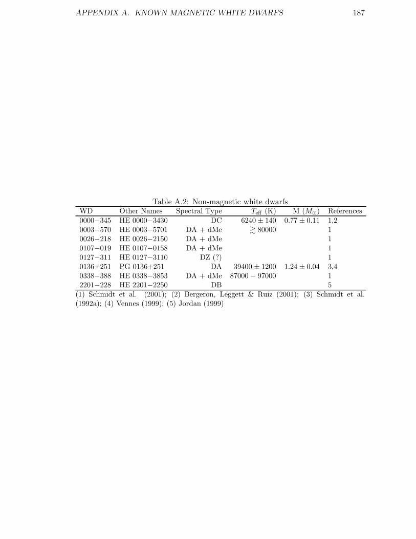
APPENDIX A. KNOWN MAGNETIC WHITE DWARFS 187
Table A.2: Non-magnetic white dwarfsWD Other Names Spectral Type Teff (K) M (M�) References0000−345 HE 0000−3430 DC 6240 ± 140 0.77 ± 0.11 1,20003−570 HE 0003−5701 DA + dMe � 80000 10026−218 HE 0026−2150 DA + dMe 10107−019 HE 0107−0158 DA + dMe 10127−311 HE 0127−3110 DZ (?) 10136+251 PG 0136+251 DA 39400 ± 1200 1.24 ± 0.04 3,40338−388 HE 0338−3853 DA + dMe 87000 − 97000 12201−228 HE 2201−2250 DB 5
(1) Schmidt et al. (2001); (2) Bergeron, Leggett & Ruiz (2001); (3) Schmidt et al.(1992a); (4) Vennes (1999); (5) Jordan (1999)
Appendix B
Tables of Models
Model atmospheres for effective temperatures ranging from 4500 K to 12000 K for
log g = 7, 8 and 9 are presented in Tables B.1 to B.18. The tables give the Rosseland
optical depth (τR), mass (m), temperature (T ), total gas pressure (Pg), electron
pressure (Pe), and the fraction of flux transported by convection (Fconv
Ftotal).
The Rosseland optical depth in the atmosphere is defined with Rosseland mean
opacities. The mass is derived from the hydrostatic equilibrium equation, where
dm = −ρ dz is intergrated to obtain m. The last column gives the fraction of
flux that is transported via convective energy transfer where the total flux that is
transfered is defined as Ftotal = Fconv + Fradiative.
Models with Teff ≥ 7000 were calculated with line-blanketing. Models with
Teff < 7000 do not include line-blanketing. Line-blanketing refers to the effect of
including line opacities in the model atmosphere calculations which has the effect
of increasing the temperature in the deeper layers of the atmosphere, i.e., below
the layers where most of the absorption lines are formed, and then of cooling the
outer layers of the atmosphere. The effect of line-blanketing in cool white dwarf
atmospheres is almost negligible and therefore was not included in the corresponding
models.
188

APPENDIX B. TABLES OF MODELS 189
Table B.1: Teff = 4500 K, log g = 7, pure H (non-blanketed)
τR m T Pg Pe
FconvFtotal
(g cm−2) (K) (dyn cm−2) (dyn cm−2)1.000E−06 6.971E−03 3713.7 6.973E+04 2.589E−03 0.0001.585E−06 9.496E−03 3713.8 9.499E+04 3.023E−03 0.0002.512E−06 1.292E−02 3714.0 1.293E+05 3.530E−03 0.0003.981E−06 1.757E−02 3714.2 1.758E+05 4.122E−03 0.0006.310E−06 2.388E−02 3714.5 2.389E+05 4.815E−03 0.0001.000E−05 3.244E−02 3715.0 3.246E+05 5.629E−03 0.0001.585E−05 4.405E−02 3715.7 4.407E+05 6.585E−03 0.0002.512E−05 5.977E−02 3716.5 5.979E+05 7.711E−03 0.0003.981E−05 8.105E−02 3717.6 8.108E+05 9.036E−03 0.0006.310E−05 1.098E−01 3718.7 1.099E+06 1.059E−02 0.0001.000E−04 1.488E−01 3720.0 1.488E+06 1.242E−02 0.0001.585E−04 2.014E−01 3721.3 2.015E+06 1.457E−02 0.0002.512E−04 2.725E−01 3722.7 2.726E+06 1.709E−02 0.0003.981E−04 3.687E−01 3724.0 3.688E+06 2.004E−02 0.0006.310E−04 4.987E−01 3725.5 4.989E+06 2.351E−02 0.0001.000E−03 6.742E−01 3727.5 6.744E+06 2.767E−02 0.0001.585E−03 9.101E−01 3730.6 9.104E+06 3.274E−02 0.0002.512E−03 1.225E+00 3735.4 1.226E+07 3.911E−02 0.0003.981E−03 1.641E+00 3743.0 1.642E+07 4.736E−02 0.0006.310E−03 2.182E+00 3754.6 2.183E+07 5.853E−02 0.0001.000E−02 2.868E+00 3772.6 2.869E+07 7.462E−02 0.0001.585E−02 3.709E+00 3799.5 3.711E+07 9.930E−02 0.0002.512E−02 4.696E+00 3838.6 4.698E+07 1.398E−01 0.0003.981E−02 5.418E+00 3970.0 5.420E+07 3.059E−01 0.0006.310E−02 6.081E+00 4129.1 6.083E+07 7.398E−01 0.0011.000E−01 6.517E+00 4244.0 6.520E+07 1.314E+00 0.0141.585E−01 6.985E+00 4362.1 6.988E+07 2.333E+00 0.0272.512E−01 7.480E+00 4482.2 7.483E+07 4.097E+00 0.0493.981E−01 7.965E+00 4595.5 7.968E+07 6.664E+00 0.1296.310E−01 8.482E+00 4711.7 8.485E+07 1.084E+01 0.2081.000E+00 9.032E+00 4830.9 9.036E+07 1.764E+01 0.2881.585E+00 9.647E+00 4959.3 9.651E+07 2.850E+01 0.4222.512E+00 1.031E+01 5091.8 1.031E+08 4.601E+01 0.5623.981E+00 1.101E+01 5227.8 1.102E+08 7.429E+01 0.7026.310E+00 1.182E+01 5377.8 1.183E+08 1.206E+02 0.7811.000E+01 1.270E+01 5534.1 1.271E+08 1.960E+02 0.8491.585E+01 1.366E+01 5695.5 1.366E+08 3.187E+02 0.9152.512E+01 1.477E+01 5875.6 1.477E+08 5.220E+02 0.9343.981E+01 1.597E+01 6061.4 1.598E+08 8.550E+02 0.9546.310E+01 1.733E+01 6260.9 1.733E+08 1.405E+03 0.9681.000E+02 1.886E+01 6475.8 1.887E+08 2.317E+03 0.975

APPENDIX B. TABLES OF MODELS 190
Table B.2: Teff = 5000 K, log g = 7, pure H (non-blanketed)
τR m T Pg Pe
FconvFtotal
(g cm−2) (K) (dyn cm−2) (dyn cm−2)1.000E−06 1.946E−03 4082.6 1.947E+04 1.051E−02 0.0001.585E−06 2.683E−03 4082.7 2.684E+04 1.235E−02 0.0002.512E−06 3.679E−03 4082.8 3.680E+04 1.447E−02 0.0003.981E−06 5.027E−03 4083.1 5.029E+04 1.694E−02 0.0006.310E−06 6.855E−03 4083.5 6.858E+04 1.982E−02 0.0001.000E−05 9.329E−03 4084.1 9.332E+04 2.318E−02 0.0001.585E−05 1.268E−02 4084.9 1.269E+05 2.714E−02 0.0002.512E−05 1.723E−02 4085.9 1.724E+05 3.180E−02 0.0003.981E−05 2.337E−02 4087.1 2.338E+05 3.726E−02 0.0006.310E−05 3.169E−02 4088.4 3.171E+05 4.368E−02 0.0001.000E−04 4.295E−02 4089.8 4.297E+05 5.121E−02 0.0001.585E−04 5.818E−02 4091.3 5.821E+05 6.003E−02 0.0002.512E−04 7.880E−02 4092.6 7.883E+05 7.034E−02 0.0003.981E−04 1.067E−01 4093.8 1.068E+06 8.236E−02 0.0006.310E−04 1.445E−01 4095.1 1.446E+06 9.646E−02 0.0001.000E−03 1.957E−01 4096.9 1.957E+06 1.132E−01 0.0001.585E−03 2.647E−01 4099.6 2.648E+06 1.335E−01 0.0002.512E−03 3.573E−01 4103.8 3.574E+06 1.584E−01 0.0003.981E−03 4.808E−01 4110.4 4.810E+06 1.899E−01 0.0006.310E−03 6.436E−01 4120.7 6.438E+06 2.312E−01 0.0001.000E−02 8.546E−01 4136.6 8.549E+06 2.882E−01 0.0001.585E−02 1.122E+00 4160.8 1.122E+07 3.716E−01 0.0002.512E−02 1.447E+00 4197.4 1.447E+07 5.036E−01 0.0003.981E−02 1.825E+00 4250.6 1.826E+07 7.268E−01 0.0006.310E−02 2.134E+00 4425.5 2.135E+07 1.712E+00 0.0001.000E−01 2.378E+00 4598.4 2.379E+07 3.695E+00 0.0071.585E−01 2.593E+00 4759.0 2.594E+07 7.194E+00 0.0172.512E−01 2.809E+00 4913.0 2.810E+07 1.313E+01 0.0503.981E−01 3.020E+00 5056.9 3.021E+07 2.219E+01 0.1096.310E−01 3.246E+00 5205.1 3.248E+07 3.749E+01 0.1681.000E+00 3.492E+00 5359.6 3.493E+07 6.212E+01 0.2901.585E+00 3.757E+00 5519.3 3.758E+07 1.022E+02 0.4322.512E+00 4.042E+00 5684.0 4.044E+07 1.683E+02 0.5733.981E+00 4.371E+00 5865.3 4.373E+07 2.767E+02 0.6776.310E+00 4.726E+00 6052.4 4.728E+07 4.550E+02 0.7821.000E+01 5.124E+00 6252.0 5.126E+07 7.494E+02 0.8571.585E+01 5.576E+00 6467.1 5.578E+07 1.237E+03 0.8932.512E+01 6.068E+00 6690.1 6.071E+07 2.040E+03 0.9283.981E+01 6.648E+00 6937.6 6.651E+07 3.375E+03 0.9446.310E+01 7.283E+00 7194.4 7.286E+07 5.583E+03 0.9601.000E+02 8.022E+00 7474.6 8.025E+07 9.229E+03 0.969

APPENDIX B. TABLES OF MODELS 191
Table B.3: Teff = 6000 K, log g = 7, pure H (non-blanketed)
τR m T Pg Pe
FconvFtotal
(g cm−2) (K) (dyn cm−2) (dyn cm−2)1.000E−06 3.326E−04 4796.9 3.327E+03 9.465E−02 0.0001.585E−06 4.628E−04 4795.8 4.629E+03 1.112E−01 0.0002.512E−06 6.391E−04 4795.0 6.393E+03 1.303E−01 0.0003.981E−06 8.783E−04 4794.5 8.787E+03 1.525E−01 0.0006.310E−06 1.203E−03 4794.4 1.203E+04 1.784E−01 0.0001.000E−05 1.644E−03 4794.7 1.645E+04 2.087E−01 0.0001.585E−05 2.242E−03 4795.4 2.243E+04 2.444E−01 0.0002.512E−05 3.053E−03 4796.4 3.054E+04 2.862E−01 0.0003.981E−05 4.152E−03 4797.6 4.154E+04 3.352E−01 0.0006.310E−05 5.642E−03 4798.9 5.645E+04 3.927E−01 0.0001.000E−04 7.662E−03 4800.3 7.665E+04 4.600E−01 0.0001.585E−04 1.040E−02 4801.6 1.041E+05 5.386E−01 0.0002.512E−04 1.412E−02 4802.6 1.412E+05 6.298E−01 0.0003.981E−04 1.916E−02 4803.5 1.917E+05 7.360E−01 0.0006.310E−04 2.601E−02 4804.5 2.602E+05 8.606E−01 0.0001.000E−03 3.529E−02 4806.0 3.531E+05 1.008E+00 0.0001.585E−03 4.785E−02 4808.6 4.786E+05 1.185E+00 0.0002.512E−03 6.479E−02 4812.7 6.481E+05 1.400E+00 0.0003.981E−03 8.753E−02 4819.2 8.756E+05 1.667E+00 0.0006.310E−03 1.178E−01 4829.5 1.179E+06 2.007E+00 0.0001.000E−02 1.577E−01 4845.4 1.578E+06 2.461E+00 0.0001.585E−02 2.094E−01 4870.3 2.095E+06 3.101E+00 0.0002.512E−02 2.747E−01 4907.8 2.748E+06 4.059E+00 0.0003.981E−02 3.546E−01 4963.5 3.547E+06 5.603E+00 0.0006.310E−02 4.479E−01 5044.5 4.481E+06 8.295E+00 0.0001.000E−01 5.506E−01 5177.8 5.509E+06 1.422E+01 0.0001.585E−01 6.358E−01 5481.6 6.361E+06 3.820E+01 0.0122.512E−01 7.083E−01 5724.8 7.086E+06 7.849E+01 0.0493.981E−01 7.789E−01 5950.5 7.792E+06 1.457E+02 0.1176.310E−01 8.521E−01 6175.0 8.524E+06 2.586E+02 0.2421.000E+00 9.301E−01 6404.0 9.305E+06 4.466E+02 0.3741.585E+00 1.015E+00 6641.4 1.015E+07 7.587E+02 0.5112.512E+00 1.108E+00 6889.3 1.109E+07 1.272E+03 0.6283.981E+00 1.213E+00 7150.2 1.213E+07 2.115E+03 0.7266.310E+00 1.329E+00 7424.5 1.330E+07 3.493E+03 0.7961.000E+01 1.461E+00 7714.6 1.462E+07 5.719E+03 0.8431.585E+01 1.611E+00 8020.4 1.611E+07 9.295E+03 0.8812.512E+01 1.779E+00 8341.4 1.780E+07 1.503E+04 0.9113.981E+01 1.975E+00 8680.4 1.976E+07 2.400E+04 0.9326.310E+01 2.199E+00 9034.7 2.200E+07 3.803E+04 0.9481.000E+02 2.456E+00 9405.3 2.457E+07 5.972E+04 0.962

APPENDIX B. TABLES OF MODELS 192
Table B.4: Teff = 8000 K, log g = 7, pure H (line-blanketed)
τR m T Pg Pe
FconvFtotal
(g cm−2) (K) (dyn cm−2) (dyn cm−2)1.000E−06 9.934E−06 6715.1 9.938E+01 2.667E+00 0.0001.585E−06 1.521E−05 6693.4 1.522E+02 3.184E+00 0.0002.512E−06 2.326E−05 6669.2 2.327E+02 3.774E+00 0.0003.981E−06 3.540E−05 6643.1 3.542E+02 4.439E+00 0.0006.310E−06 5.350E−05 6615.5 5.352E+02 5.182E+00 0.0001.000E−05 8.027E−05 6586.7 8.030E+02 6.005E+00 0.0001.585E−05 1.196E−04 6557.3 1.196E+03 6.918E+00 0.0002.512E−05 1.771E−04 6527.4 1.771E+03 7.932E+00 0.0003.981E−05 2.608E−04 6497.0 2.609E+03 9.055E+00 0.0006.310E−05 3.824E−04 6466.7 3.825E+03 1.030E+01 0.0001.000E−04 5.583E−04 6437.8 5.585E+03 1.173E+01 0.0001.585E−04 8.111E−04 6411.7 8.114E+03 1.339E+01 0.0002.512E−04 1.172E−03 6389.0 1.172E+04 1.534E+01 0.0003.981E−04 1.683E−03 6369.7 1.684E+04 1.764E+01 0.0006.310E−04 2.403E−03 6353.7 2.404E+04 2.038E+01 0.0001.000E−03 3.412E−03 6341.1 3.413E+04 2.363E+01 0.0001.585E−03 4.813E−03 6332.0 4.815E+04 2.752E+01 0.0002.512E−03 6.752E−03 6327.1 6.754E+04 3.226E+01 0.0003.981E−03 9.412E−03 6327.1 9.416E+04 3.809E+01 0.0006.310E−03 1.303E−02 6333.5 1.304E+05 4.545E+01 0.0001.000E−02 1.791E−02 6348.7 1.792E+05 5.506E+01 0.0001.585E−02 2.438E−02 6376.6 2.439E+05 6.820E+01 0.0002.512E−02 3.281E−02 6422.6 3.282E+05 8.723E+01 0.0003.981E−02 4.347E−02 6493.9 4.349E+05 1.165E+02 0.0006.310E−02 5.651E−02 6600.7 5.653E+05 1.651E+02 0.0001.000E−01 7.174E−02 6753.8 7.177E+05 2.509E+02 0.0001.585E−01 8.851E−02 6985.6 8.854E+05 4.281E+02 0.0002.512E−01 1.045E−01 7404.8 1.046E+06 9.486E+02 0.0053.981E−01 1.180E−01 7848.0 1.181E+06 1.973E+03 0.0386.310E−01 1.308E−01 8286.2 1.308E+06 3.790E+03 0.1251.000E+00 1.429E−01 8686.5 1.430E+06 6.502E+03 0.2651.585E+00 1.555E−01 9055.5 1.556E+06 1.033E+04 0.4392.512E+00 1.692E−01 9405.4 1.693E+06 1.560E+04 0.6373.981E+00 1.847E−01 9736.5 1.848E+06 2.256E+04 0.7496.310E+00 2.026E−01 10059.4 2.026E+06 3.182E+04 0.8451.000E+01 2.236E−01 10379.6 2.237E+06 4.410E+04 0.8911.585E+01 2.487E−01 10700.6 2.488E+06 6.039E+04 0.9232.512E+01 2.789E−01 11025.7 2.790E+06 8.206E+04 0.9443.981E+01 3.157E−01 11357.5 3.158E+06 1.109E+05 0.9606.310E+01 3.607E−01 11698.4 3.608E+06 1.496E+05 0.9711.000E+02 4.161E−01 12050.0 4.162E+06 2.013E+05 0.979

APPENDIX B. TABLES OF MODELS 193
Table B.5: Teff = 10000 K, log g = 7, pure H (line-blanketed)
τR m T Pg Pe
FconvFtotal
(g cm−2) (K) (dyn cm−2) (dyn cm−2)1.000E−06 1.507E−06 7842.5 1.507E+01 4.477E+00 0.0001.585E−06 2.121E−06 7902.4 2.122E+01 5.992E+00 0.0002.512E−06 2.987E−06 7943.2 2.988E+01 7.862E+00 0.0003.981E−06 4.241E−06 7961.3 4.243E+01 1.010E+01 0.0006.310E−06 6.115E−06 7957.9 6.118E+01 1.274E+01 0.0001.000E−05 8.982E−06 7942.8 8.985E+01 1.591E+01 0.0001.585E−05 1.341E−05 7925.0 1.342E+02 1.980E+01 0.0002.512E−05 2.026E−05 7907.7 2.027E+02 2.461E+01 0.0003.981E−05 3.080E−05 7891.3 3.081E+02 3.051E+01 0.0006.310E−05 4.689E−05 7875.8 4.691E+02 3.767E+01 0.0001.000E−04 7.130E−05 7859.4 7.133E+02 4.621E+01 0.0001.585E−04 1.083E−04 7839.7 1.083E+03 5.617E+01 0.0002.512E−04 1.642E−04 7815.8 1.643E+03 6.762E+01 0.0003.981E−04 2.483E−04 7796.4 2.484E+03 8.155E+01 0.0006.310E−04 3.724E−04 7783.0 3.726E+03 9.861E+01 0.0001.000E−03 5.533E−04 7774.3 5.535E+03 1.193E+02 0.0001.585E−03 8.126E−04 7778.2 8.129E+03 1.459E+02 0.0002.512E−03 1.177E−03 7794.0 1.177E+04 1.802E+02 0.0003.981E−03 1.680E−03 7821.0 1.681E+04 2.244E+02 0.0006.310E−03 2.367E−03 7856.0 2.368E+04 2.806E+02 0.0001.000E−02 3.301E−03 7894.5 3.302E+04 3.506E+02 0.0001.585E−02 4.558E−03 7946.6 4.560E+04 4.440E+02 0.0002.512E−02 6.212E−03 8021.7 6.215E+04 5.758E+02 0.0003.981E−02 8.323E−03 8129.3 8.326E+04 7.720E+02 0.0006.310E−02 1.090E−02 8278.5 1.091E+05 1.076E+03 0.0001.000E−01 1.394E−02 8470.0 1.394E+05 1.551E+03 0.0001.585E−01 1.734E−02 8726.8 1.734E+05 2.355E+03 0.0002.512E−01 2.074E−02 9154.2 2.075E+05 4.144E+03 0.0013.981E−01 2.342E−02 9828.9 2.343E+05 8.532E+03 0.0186.310E−01 2.554E−02 10486.7 2.555E+05 1.559E+04 0.0821.000E+00 2.754E−02 11000.7 2.755E+05 2.370E+04 0.2611.585E+00 2.971E−02 11435.6 2.972E+05 3.291E+04 0.4342.512E+00 3.223E−02 11836.5 3.224E+05 4.375E+04 0.6213.981E+00 3.530E−02 12224.4 3.531E+05 5.680E+04 0.7536.310E+00 3.916E−02 12610.2 3.917E+05 7.284E+04 0.8331.000E+01 4.407E−02 13006.3 4.408E+05 9.308E+04 0.8871.585E+01 5.044E−02 13420.0 5.045E+05 1.191E+05 0.9182.512E+01 5.873E−02 13857.7 5.875E+05 1.530E+05 0.9393.981E+01 6.968E−02 14326.4 6.969E+05 1.978E+05 0.9546.310E+01 8.406E−02 14829.8 8.408E+05 2.575E+05 0.9651.000E+02 1.032E−01 15374.1 1.032E+06 3.377E+05 0.973

APPENDIX B. TABLES OF MODELS 194
Table B.6: Teff = 12000 K, log g = 7, pure H (line-blanketed)
τR m T Pg Pe
FconvFtotal
(g cm−2) (K) (dyn cm−2) (dyn cm−2)1.000E−06 1.028E−06 8505.8 1.029E+01 4.596E+00 0.0001.585E−06 1.437E−06 8592.0 1.437E+01 6.342E+00 0.0002.512E−06 1.983E−06 8680.8 1.983E+01 8.649E+00 0.0003.981E−06 2.710E−06 8766.4 2.711E+01 1.167E+01 0.0006.310E−06 3.677E−06 8842.7 3.679E+01 1.558E+01 0.0001.000E−05 4.966E−06 8902.9 4.967E+01 2.056E+01 0.0001.585E−05 6.694E−06 8940.1 6.697E+01 2.681E+01 0.0002.512E−05 9.045E−06 8947.9 9.049E+01 3.442E+01 0.0003.981E−05 1.231E−05 8931.4 1.231E+02 4.356E+01 0.0006.310E−05 1.694E−05 8904.6 1.695E+02 5.466E+01 0.0001.000E−04 2.366E−05 8877.1 2.367E+02 6.831E+01 0.0001.585E−04 3.349E−05 8854.3 3.351E+02 8.532E+01 0.0002.512E−04 4.799E−05 8836.7 4.801E+02 1.065E+02 0.0003.981E−04 6.951E−05 8818.5 6.953E+02 1.325E+02 0.0006.310E−04 1.015E−04 8810.3 1.015E+03 1.655E+02 0.0001.000E−03 1.484E−04 8820.9 1.485E+03 2.091E+02 0.0001.585E−03 2.151E−04 8855.1 2.151E+03 2.677E+02 0.0002.512E−03 3.078E−04 8904.4 3.079E+03 3.445E+02 0.0003.981E−03 4.354E−04 8959.0 4.356E+03 4.417E+02 0.0006.310E−03 6.104E−04 9019.0 6.106E+03 5.653E+02 0.0001.000E−02 8.477E−04 9093.6 8.480E+03 7.290E+02 0.0001.585E−02 1.161E−03 9199.9 1.162E+04 9.608E+02 0.0002.512E−02 1.562E−03 9330.5 1.562E+04 1.280E+03 0.0003.981E−02 2.067E−03 9472.4 2.067E+04 1.702E+03 0.0006.310E−02 2.701E−03 9638.3 2.701E+04 2.289E+03 0.0001.000E−01 3.471E−03 9857.3 3.472E+04 3.175E+03 0.0001.585E−01 4.361E−03 10157.0 4.362E+04 4.598E+03 0.0002.512E−01 5.311E−03 10580.1 5.312E+04 7.027E+03 0.0003.981E−01 6.267E−03 11164.9 6.267E+04 1.124E+04 0.0016.310E−01 7.200E−03 11922.7 7.200E+04 1.797E+04 0.0071.000E+00 8.200E−03 12799.7 8.199E+04 2.707E+04 0.0161.585E+00 9.434E−03 13866.2 9.430E+04 3.830E+04 0.0142.512E+00 1.132E−02 15179.0 1.131E+05 5.153E+04 0.0013.981E+00 1.462E−02 16677.7 1.461E+05 7.002E+04 0.0006.310E+00 2.065E−02 18397.6 2.063E+05 1.008E+05 0.0001.000E+01 3.108E−02 20382.5 3.105E+05 1.529E+05 0.0001.585E+01 4.813E−02 22666.2 4.808E+05 2.375E+05 0.0002.512E+01 7.470E−02 25277.4 7.462E+05 3.689E+05 0.0003.981E+01 1.147E−01 28244.3 1.146E+06 5.661E+05 0.0006.310E+01 1.735E−01 31601.7 1.733E+06 8.560E+05 0.0001.000E+02 2.602E−01 35394.5 2.599E+06 1.282E+06 0.000
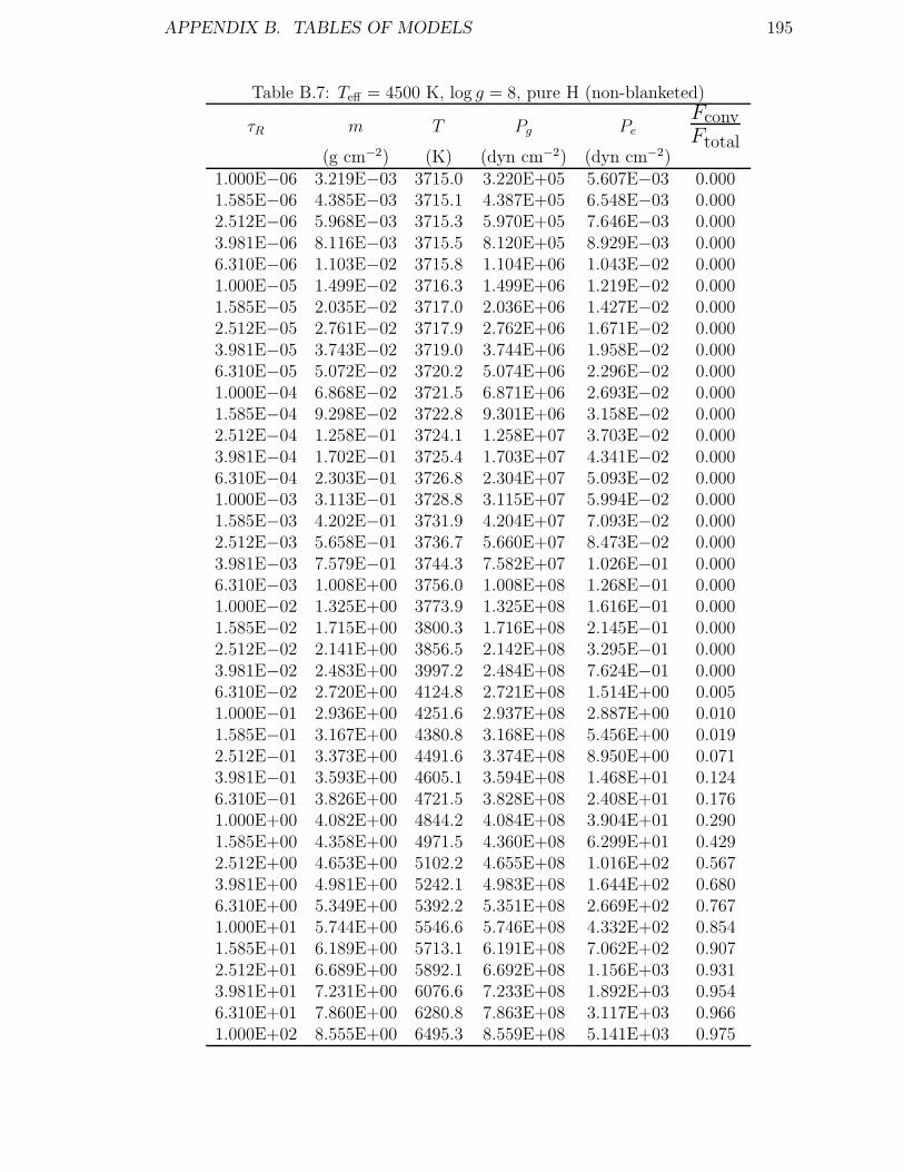
APPENDIX B. TABLES OF MODELS 195
Table B.7: Teff = 4500 K, log g = 8, pure H (non-blanketed)
τR m T Pg Pe
FconvFtotal
(g cm−2) (K) (dyn cm−2) (dyn cm−2)1.000E−06 3.219E−03 3715.0 3.220E+05 5.607E−03 0.0001.585E−06 4.385E−03 3715.1 4.387E+05 6.548E−03 0.0002.512E−06 5.968E−03 3715.3 5.970E+05 7.646E−03 0.0003.981E−06 8.116E−03 3715.5 8.120E+05 8.929E−03 0.0006.310E−06 1.103E−02 3715.8 1.104E+06 1.043E−02 0.0001.000E−05 1.499E−02 3716.3 1.499E+06 1.219E−02 0.0001.585E−05 2.035E−02 3717.0 2.036E+06 1.427E−02 0.0002.512E−05 2.761E−02 3717.9 2.762E+06 1.671E−02 0.0003.981E−05 3.743E−02 3719.0 3.744E+06 1.958E−02 0.0006.310E−05 5.072E−02 3720.2 5.074E+06 2.296E−02 0.0001.000E−04 6.868E−02 3721.5 6.871E+06 2.693E−02 0.0001.585E−04 9.298E−02 3722.8 9.301E+06 3.158E−02 0.0002.512E−04 1.258E−01 3724.1 1.258E+07 3.703E−02 0.0003.981E−04 1.702E−01 3725.4 1.703E+07 4.341E−02 0.0006.310E−04 2.303E−01 3726.8 2.304E+07 5.093E−02 0.0001.000E−03 3.113E−01 3728.8 3.115E+07 5.994E−02 0.0001.585E−03 4.202E−01 3731.9 4.204E+07 7.093E−02 0.0002.512E−03 5.658E−01 3736.7 5.660E+07 8.473E−02 0.0003.981E−03 7.579E−01 3744.3 7.582E+07 1.026E−01 0.0006.310E−03 1.008E+00 3756.0 1.008E+08 1.268E−01 0.0001.000E−02 1.325E+00 3773.9 1.325E+08 1.616E−01 0.0001.585E−02 1.715E+00 3800.3 1.716E+08 2.145E−01 0.0002.512E−02 2.141E+00 3856.5 2.142E+08 3.295E−01 0.0003.981E−02 2.483E+00 3997.2 2.484E+08 7.624E−01 0.0006.310E−02 2.720E+00 4124.8 2.721E+08 1.514E+00 0.0051.000E−01 2.936E+00 4251.6 2.937E+08 2.887E+00 0.0101.585E−01 3.167E+00 4380.8 3.168E+08 5.456E+00 0.0192.512E−01 3.373E+00 4491.6 3.374E+08 8.950E+00 0.0713.981E−01 3.593E+00 4605.1 3.594E+08 1.468E+01 0.1246.310E−01 3.826E+00 4721.5 3.828E+08 2.408E+01 0.1761.000E+00 4.082E+00 4844.2 4.084E+08 3.904E+01 0.2901.585E+00 4.358E+00 4971.5 4.360E+08 6.299E+01 0.4292.512E+00 4.653E+00 5102.2 4.655E+08 1.016E+02 0.5673.981E+00 4.981E+00 5242.1 4.983E+08 1.644E+02 0.6806.310E+00 5.349E+00 5392.2 5.351E+08 2.669E+02 0.7671.000E+01 5.744E+00 5546.6 5.746E+08 4.332E+02 0.8541.585E+01 6.189E+00 5713.1 6.191E+08 7.062E+02 0.9072.512E+01 6.689E+00 5892.1 6.692E+08 1.156E+03 0.9313.981E+01 7.231E+00 6076.6 7.233E+08 1.892E+03 0.9546.310E+01 7.860E+00 6280.8 7.863E+08 3.117E+03 0.9661.000E+02 8.555E+00 6495.3 8.559E+08 5.141E+03 0.975

APPENDIX B. TABLES OF MODELS 196
Table B.8: Teff = 5000 K, log g = 8, pure H (non-blanketed)
τR m T Pg Pe
FconvFtotal
(g cm−2) (K) (dyn cm−2) (dyn cm−2)1.000E−06 8.991E−04 4083.6 8.995E+04 2.270E−02 0.0001.585E−06 1.241E−03 4083.7 1.241E+05 2.668E−02 0.0002.512E−06 1.702E−03 4083.9 1.703E+05 3.128E−02 0.0003.981E−06 2.326E−03 4084.1 2.327E+05 3.662E−02 0.0006.310E−06 3.172E−03 4084.6 3.173E+05 4.286E−02 0.0001.000E−05 4.318E−03 4085.2 4.320E+05 5.017E−02 0.0001.585E−05 5.869E−03 4086.1 5.872E+05 5.875E−02 0.0002.512E−05 7.969E−03 4087.3 7.973E+05 6.886E−02 0.0003.981E−05 1.081E−02 4088.6 1.081E+06 8.075E−02 0.0006.310E−05 1.465E−02 4090.1 1.466E+06 9.471E−02 0.0001.000E−04 1.985E−02 4091.6 1.985E+06 1.111E−01 0.0001.585E−04 2.688E−02 4093.0 2.689E+06 1.301E−01 0.0002.512E−04 3.640E−02 4094.1 3.641E+06 1.523E−01 0.0003.981E−04 4.930E−02 4095.2 4.932E+06 1.783E−01 0.0006.310E−04 6.678E−02 4096.5 6.681E+06 2.088E−01 0.0001.000E−03 9.043E−02 4098.3 9.047E+06 2.451E−01 0.0001.585E−03 1.223E−01 4101.0 1.224E+07 2.890E−01 0.0002.512E−03 1.652E−01 4105.2 1.652E+07 3.429E−01 0.0003.981E−03 2.222E−01 4111.8 2.223E+07 4.112E−01 0.0006.310E−03 2.975E−01 4122.2 2.976E+07 5.007E−01 0.0001.000E−02 3.951E−01 4138.1 3.952E+07 6.242E−01 0.0001.585E−02 5.184E−01 4162.5 5.186E+07 8.054E−01 0.0002.512E−02 6.686E−01 4199.3 6.689E+07 1.092E+00 0.0003.981E−02 8.414E−01 4259.2 8.417E+07 1.623E+00 0.0006.310E−02 9.849E−01 4443.2 9.853E+07 3.984E+00 0.0001.000E−01 1.084E+00 4615.1 1.084E+08 8.430E+00 0.0061.585E−01 1.186E+00 4782.3 1.186E+08 1.686E+01 0.0202.512E−01 1.277E+00 4924.9 1.278E+08 2.908E+01 0.0563.981E−01 1.375E+00 5071.7 1.376E+08 5.014E+01 0.0936.310E−01 1.479E+00 5220.3 1.480E+08 8.352E+01 0.1911.000E+00 1.590E+00 5372.4 1.590E+08 1.376E+02 0.3081.585E+00 1.709E+00 5529.5 1.710E+08 2.266E+02 0.4272.512E+00 1.845E+00 5700.4 1.846E+08 3.716E+02 0.5593.981E+00 1.992E+00 5876.6 1.993E+08 6.094E+02 0.6926.310E+00 2.156E+00 6064.4 2.157E+08 1.001E+03 0.7921.000E+01 2.342E+00 6267.0 2.343E+08 1.649E+03 0.8461.585E+01 2.544E+00 6476.5 2.545E+08 2.716E+03 0.9012.512E+01 2.781E+00 6709.3 2.782E+08 4.493E+03 0.9243.981E+01 3.041E+00 6951.9 3.042E+08 7.435E+03 0.9456.310E+01 3.340E+00 7214.8 3.341E+08 1.233E+04 0.9591.000E+02 3.679E+00 7496.0 3.681E+08 2.046E+04 0.969

APPENDIX B. TABLES OF MODELS 197
Table B.9: Teff = 6000 K, log g = 8, pure H (non-blanketed)
τR m T Pg Pe
FconvFtotal
(g cm−2) (K) (dyn cm−2) (dyn cm−2)1.000E−06 1.578E−04 4792.3 1.579E+04 2.027E−01 0.0001.585E−06 2.191E−04 4791.9 2.192E+04 2.384E−01 0.0002.512E−06 3.018E−04 4791.7 3.020E+04 2.797E−01 0.0003.981E−06 4.139E−04 4791.7 4.141E+04 3.276E−01 0.0006.310E−06 5.658E−04 4792.1 5.660E+04 3.835E−01 0.0001.000E−05 7.718E−04 4792.8 7.721E+04 4.490E−01 0.0001.585E−05 1.051E−03 4793.8 1.051E+05 5.259E−01 0.0002.512E−05 1.428E−03 4795.2 1.429E+05 6.162E−01 0.0003.981E−05 1.940E−03 4796.7 1.941E+05 7.224E−01 0.0006.310E−05 2.633E−03 4798.3 2.634E+05 8.466E−01 0.0001.000E−04 3.573E−03 4799.9 3.574E+05 9.918E−01 0.0001.585E−04 4.847E−03 4801.2 4.848E+05 1.161E+00 0.0002.512E−04 6.572E−03 4802.2 6.574E+05 1.357E+00 0.0003.981E−04 8.916E−03 4803.2 8.919E+05 1.586E+00 0.0006.310E−04 1.210E−02 4804.3 1.210E+06 1.855E+00 0.0001.000E−03 1.641E−02 4805.9 1.642E+06 2.174E+00 0.0001.585E−03 2.224E−02 4808.6 2.225E+06 2.555E+00 0.0002.512E−03 3.010E−02 4812.7 3.011E+06 3.018E+00 0.0003.981E−03 4.066E−02 4819.3 4.068E+06 3.593E+00 0.0006.310E−03 5.472E−02 4829.6 5.474E+06 4.328E+00 0.0001.000E−02 7.325E−02 4845.6 7.328E+06 5.307E+00 0.0001.585E−02 9.721E−02 4870.5 9.725E+06 6.687E+00 0.0002.512E−02 1.275E−01 4908.1 1.276E+07 8.757E+00 0.0003.981E−02 1.646E−01 4963.8 1.647E+07 1.208E+01 0.0006.310E−02 2.079E−01 5045.1 2.080E+07 1.791E+01 0.0001.000E−01 2.546E−01 5207.4 2.547E+07 3.357E+01 0.0001.585E−01 2.923E−01 5500.5 2.924E+07 8.639E+01 0.0112.512E−01 3.251E−01 5738.6 3.252E+07 1.743E+02 0.0583.981E−01 3.576E−01 5960.7 3.577E+07 3.201E+02 0.1286.310E−01 3.914E−01 6180.7 3.916E+07 5.613E+02 0.2341.000E+00 4.279E−01 6406.2 4.281E+07 9.624E+02 0.3921.585E+00 4.679E−01 6640.8 4.681E+07 1.627E+03 0.5302.512E+00 5.123E−01 6887.4 5.125E+07 2.725E+03 0.6483.981E+00 5.620E−01 7147.9 5.622E+07 4.541E+03 0.7396.310E+00 6.179E−01 7424.3 6.181E+07 7.535E+03 0.8041.000E+01 6.812E−01 7718.5 6.815E+07 1.245E+04 0.8481.585E+01 7.535E−01 8032.0 7.538E+07 2.047E+04 0.8832.512E+01 8.361E−01 8365.7 8.364E+07 3.353E+04 0.9093.981E+01 9.302E−01 8719.1 9.306E+07 5.471E+04 0.9316.310E+01 1.039E+00 9096.2 1.040E+08 8.862E+04 0.9461.000E+02 1.166E+00 9496.2 1.166E+08 1.425E+05 0.958
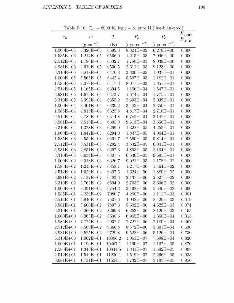
APPENDIX B. TABLES OF MODELS 198
Table B.10: Teff = 8000 K, log g = 8, pure H (line-blanketed)
τR m T Pg Pe
FconvFtotal
(g cm−2) (K) (dyn cm−2) (dyn cm−2)1.000E−06 8.320E−06 6599.3 8.324E+02 6.270E+00 0.0001.585E−06 1.214E−05 6566.0 1.215E+03 7.096E+00 0.0002.512E−06 1.780E−05 6532.7 1.780E+03 8.039E+00 0.0003.981E−06 2.610E−05 6500.5 2.611E+03 9.123E+00 0.0006.310E−06 3.818E−05 6470.3 3.820E+03 1.037E+01 0.0001.000E−05 5.565E−05 6442.4 5.567E+03 1.182E+01 0.0001.585E−05 8.073E−05 6417.3 8.077E+03 1.351E+01 0.0002.512E−05 1.165E−04 6394.5 1.166E+04 1.547E+01 0.0003.981E−05 1.673E−04 6373.7 1.674E+04 1.775E+01 0.0006.310E−05 2.392E−04 6355.2 2.393E+04 2.039E+01 0.0001.000E−04 3.401E−04 6339.2 3.403E+04 2.350E+01 0.0001.585E−04 4.815E−04 6325.8 4.817E+04 2.716E+01 0.0002.512E−04 6.782E−04 6314.8 6.785E+04 3.147E+01 0.0003.981E−04 9.510E−04 6305.9 9.513E+04 3.656E+01 0.0006.310E−04 1.328E−03 6299.0 1.328E+05 4.255E+01 0.0001.000E−03 1.847E−03 6294.0 1.847E+05 4.964E+01 0.0001.585E−03 2.559E−03 6291.7 2.560E+05 5.814E+01 0.0002.512E−03 3.531E−03 6292.4 3.532E+05 6.841E+01 0.0003.981E−03 4.851E−03 6297.3 4.853E+05 8.104E+01 0.0006.310E−03 6.634E−03 6307.6 6.636E+05 9.695E+01 0.0001.000E−02 9.018E−03 6326.7 9.021E+05 1.178E+02 0.0001.585E−02 1.216E−02 6358.1 1.217E+06 1.464E+02 0.0002.512E−02 1.623E−02 6407.6 1.624E+06 1.880E+02 0.0003.981E−02 2.137E−02 6483.3 2.137E+06 2.527E+02 0.0006.310E−02 2.762E−02 6594.9 2.763E+06 3.606E+02 0.0001.000E−01 3.491E−02 6754.2 3.492E+06 5.540E+02 0.0001.585E−01 4.259E−02 7080.7 4.260E+06 1.111E+03 0.0012.512E−01 4.940E−02 7507.6 4.942E+06 2.426E+03 0.0193.981E−01 5.600E−02 7897.3 5.602E+06 4.629E+03 0.0716.310E−01 6.260E−02 8269.3 6.263E+06 8.120E+03 0.1651.000E+00 6.963E−02 8638.6 6.965E+06 1.360E+04 0.3151.585E+00 7.724E−02 9002.7 7.727E+06 2.180E+04 0.4672.512E+00 8.569E−02 9366.8 8.572E+06 3.391E+04 0.6303.981E+00 9.525E−02 9729.8 9.528E+06 5.126E+04 0.7306.310E+00 1.062E−01 10096.2 1.063E+07 7.598E+04 0.8201.000E+01 1.190E−01 10467.1 1.190E+07 1.107E+05 0.8701.585E+01 1.340E−01 10844.5 1.341E+07 1.592E+05 0.9082.512E+01 1.519E−01 11230.1 1.519E+07 2.266E+05 0.9333.981E+01 1.731E−01 11624.1 1.732E+07 3.193E+05 0.950
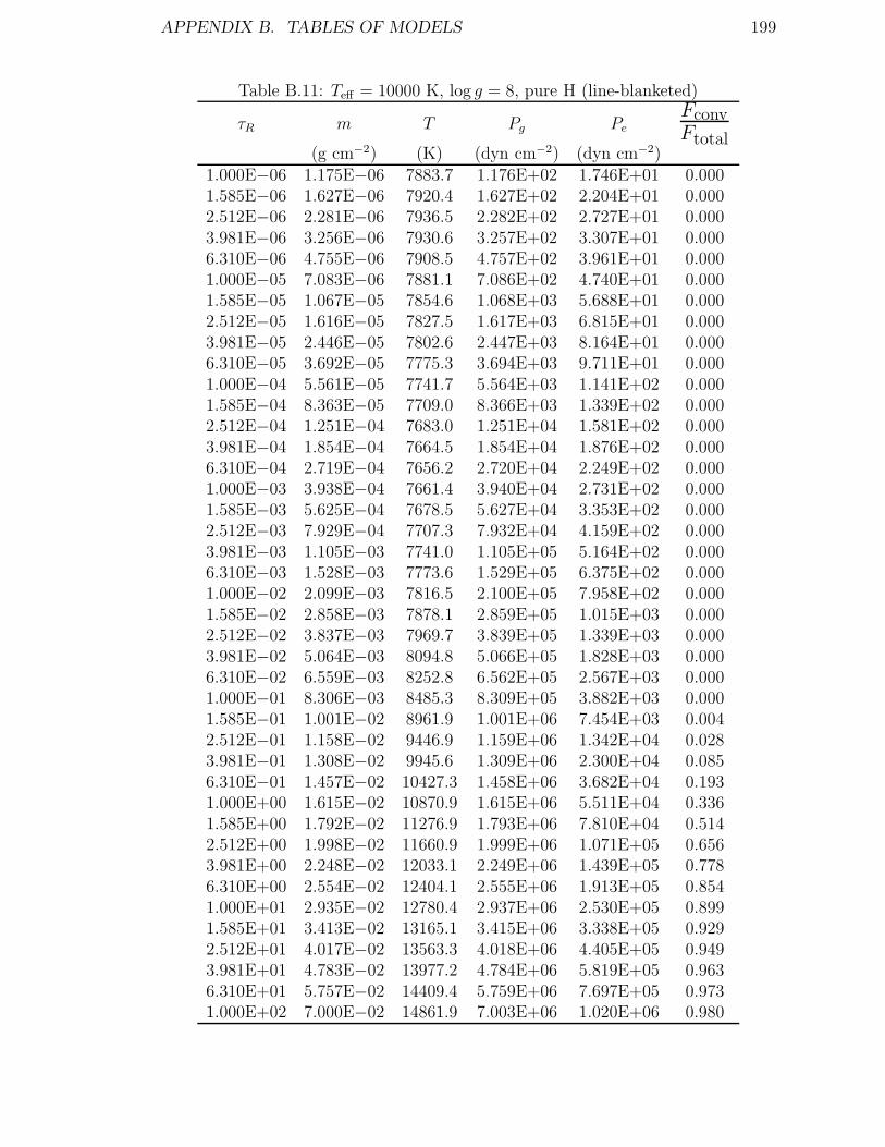
APPENDIX B. TABLES OF MODELS 199
Table B.11: Teff = 10000 K, log g = 8, pure H (line-blanketed)
τR m T Pg Pe
FconvFtotal
(g cm−2) (K) (dyn cm−2) (dyn cm−2)1.000E−06 1.175E−06 7883.7 1.176E+02 1.746E+01 0.0001.585E−06 1.627E−06 7920.4 1.627E+02 2.204E+01 0.0002.512E−06 2.281E−06 7936.5 2.282E+02 2.727E+01 0.0003.981E−06 3.256E−06 7930.6 3.257E+02 3.307E+01 0.0006.310E−06 4.755E−06 7908.5 4.757E+02 3.961E+01 0.0001.000E−05 7.083E−06 7881.1 7.086E+02 4.740E+01 0.0001.585E−05 1.067E−05 7854.6 1.068E+03 5.688E+01 0.0002.512E−05 1.616E−05 7827.5 1.617E+03 6.815E+01 0.0003.981E−05 2.446E−05 7802.6 2.447E+03 8.164E+01 0.0006.310E−05 3.692E−05 7775.3 3.694E+03 9.711E+01 0.0001.000E−04 5.561E−05 7741.7 5.564E+03 1.141E+02 0.0001.585E−04 8.363E−05 7709.0 8.366E+03 1.339E+02 0.0002.512E−04 1.251E−04 7683.0 1.251E+04 1.581E+02 0.0003.981E−04 1.854E−04 7664.5 1.854E+04 1.876E+02 0.0006.310E−04 2.719E−04 7656.2 2.720E+04 2.249E+02 0.0001.000E−03 3.938E−04 7661.4 3.940E+04 2.731E+02 0.0001.585E−03 5.625E−04 7678.5 5.627E+04 3.353E+02 0.0002.512E−03 7.929E−04 7707.3 7.932E+04 4.159E+02 0.0003.981E−03 1.105E−03 7741.0 1.105E+05 5.164E+02 0.0006.310E−03 1.528E−03 7773.6 1.529E+05 6.375E+02 0.0001.000E−02 2.099E−03 7816.5 2.100E+05 7.958E+02 0.0001.585E−02 2.858E−03 7878.1 2.859E+05 1.015E+03 0.0002.512E−02 3.837E−03 7969.7 3.839E+05 1.339E+03 0.0003.981E−02 5.064E−03 8094.8 5.066E+05 1.828E+03 0.0006.310E−02 6.559E−03 8252.8 6.562E+05 2.567E+03 0.0001.000E−01 8.306E−03 8485.3 8.309E+05 3.882E+03 0.0001.585E−01 1.001E−02 8961.9 1.001E+06 7.454E+03 0.0042.512E−01 1.158E−02 9446.9 1.159E+06 1.342E+04 0.0283.981E−01 1.308E−02 9945.6 1.309E+06 2.300E+04 0.0856.310E−01 1.457E−02 10427.3 1.458E+06 3.682E+04 0.1931.000E+00 1.615E−02 10870.9 1.615E+06 5.511E+04 0.3361.585E+00 1.792E−02 11276.9 1.793E+06 7.810E+04 0.5142.512E+00 1.998E−02 11660.9 1.999E+06 1.071E+05 0.6563.981E+00 2.248E−02 12033.1 2.249E+06 1.439E+05 0.7786.310E+00 2.554E−02 12404.1 2.555E+06 1.913E+05 0.8541.000E+01 2.935E−02 12780.4 2.937E+06 2.530E+05 0.8991.585E+01 3.413E−02 13165.1 3.415E+06 3.338E+05 0.9292.512E+01 4.017E−02 13563.3 4.018E+06 4.405E+05 0.9493.981E+01 4.783E−02 13977.2 4.784E+06 5.819E+05 0.9636.310E+01 5.757E−02 14409.4 5.759E+06 7.697E+05 0.9731.000E+02 7.000E−02 14861.9 7.003E+06 1.020E+06 0.980

APPENDIX B. TABLES OF MODELS 200
Table B.12: Teff = 12000 K, log g = 8, pure H (line-blanketed)
τR m T Pg Pe
FconvFtotal
(g cm−2) (K) (dyn cm−2) (dyn cm−2)1.000E−06 5.223E−07 8616.6 5.225E+01 1.899E+01 0.0001.585E−06 7.191E−07 8697.6 7.194E+01 2.544E+01 0.0002.512E−06 9.796E−07 8775.2 9.799E+01 3.365E+01 0.0003.981E−06 1.327E−06 8845.0 1.328E+02 4.402E+01 0.0006.310E−06 1.795E−06 8900.2 1.796E+02 5.690E+01 0.0001.000E−05 2.438E−06 8933.3 2.439E+02 7.244E+01 0.0001.585E−05 3.343E−06 8937.9 3.345E+02 9.060E+01 0.0002.512E−05 4.668E−06 8912.5 4.670E+02 1.112E+02 0.0003.981E−05 6.676E−06 8867.2 6.679E+02 1.348E+02 0.0006.310E−05 9.778E−06 8823.6 9.782E+02 1.638E+02 0.0001.000E−04 1.456E−05 8787.8 1.456E+03 2.002E+02 0.0001.585E−04 2.189E−05 8756.8 2.190E+03 2.451E+02 0.0002.512E−04 3.304E−05 8738.0 3.305E+03 3.021E+02 0.0003.981E−04 4.955E−05 8739.7 4.957E+03 3.776E+02 0.0006.310E−04 7.314E−05 8772.7 7.317E+03 4.825E+02 0.0001.000E−03 1.056E−04 8826.7 1.057E+04 6.225E+02 0.0001.585E−03 1.501E−04 8878.5 1.502E+04 7.929E+02 0.0002.512E−03 2.109E−04 8935.4 2.110E+04 1.008E+03 0.0003.981E−03 2.931E−04 9008.4 2.932E+04 1.295E+03 0.0006.310E−03 4.013E−04 9115.7 4.015E+04 1.708E+03 0.0001.000E−02 5.396E−04 9247.9 5.398E+04 2.283E+03 0.0001.585E−02 7.155E−04 9372.9 7.157E+04 2.997E+03 0.0002.512E−02 9.457E−04 9481.4 9.461E+04 3.854E+03 0.0003.981E−02 1.250E−03 9603.2 1.250E+05 5.006E+03 0.0006.310E−02 1.636E−03 9788.4 1.636E+05 6.839E+03 0.0001.000E−01 2.077E−03 10144.2 2.078E+05 1.058E+04 0.0011.585E−01 2.527E−03 10614.9 2.528E+05 1.709E+04 0.0082.512E−01 2.972E−03 11177.4 2.973E+05 2.787E+04 0.0273.981E−01 3.410E−03 11816.7 3.411E+05 4.470E+04 0.0696.310E−01 3.857E−03 12472.0 3.858E+05 6.763E+04 0.1421.000E+00 4.355E−03 13110.4 4.356E+05 9.615E+04 0.2601.585E+00 4.947E−03 13745.4 4.948E+05 1.312E+05 0.3892.512E+00 5.685E−03 14404.0 5.686E+05 1.748E+05 0.5113.981E+00 6.650E−03 15122.2 6.652E+05 2.306E+05 0.6006.310E+00 7.963E−03 15956.2 7.964E+05 3.047E+05 0.6531.000E+01 9.814E−03 17003.4 9.816E+05 4.078E+05 0.6671.585E+01 1.258E−02 18508.2 1.258E+06 5.600E+05 0.6022.512E+01 1.726E−02 21340.0 1.726E+06 8.138E+05 0.2753.981E+01 2.679E−02 25657.6 2.678E+06 1.290E+06 0.0016.310E+01 4.342E−02 29865.5 4.342E+06 2.095E+06 0.0001.000E+02 6.911E−02 34206.8 6.910E+06 3.327E+06 0.000

APPENDIX B. TABLES OF MODELS 201
Table B.13: Teff = 4500 K, log g = 9, pure H (non-blanketed)
τR m T Pg Pe
FconvFtotal
(g cm−2) (K) (dyn cm−2) (dyn cm−2)1.000E−06 1.493E−03 3715.3 1.494E+06 1.209E−02 0.0001.585E−06 2.034E−03 3715.3 2.034E+06 1.412E−02 0.0002.512E−06 2.767E−03 3715.5 2.769E+06 1.649E−02 0.0003.981E−06 3.764E−03 3715.7 3.765E+06 1.925E−02 0.0006.310E−06 5.116E−03 3716.1 5.118E+06 2.249E−02 0.0001.000E−05 6.950E−03 3716.5 6.953E+06 2.629E−02 0.0001.585E−05 9.436E−03 3717.2 9.440E+06 3.076E−02 0.0002.512E−05 1.280E−02 3718.1 1.281E+07 3.602E−02 0.0003.981E−05 1.736E−02 3719.1 1.737E+07 4.221E−02 0.0006.310E−05 2.353E−02 3720.3 2.354E+07 4.948E−02 0.0001.000E−04 3.186E−02 3721.5 3.188E+07 5.803E−02 0.0001.585E−04 4.313E−02 3722.9 4.315E+07 6.806E−02 0.0002.512E−04 5.837E−02 3724.2 5.839E+07 7.982E−02 0.0003.981E−04 7.898E−02 3725.6 7.901E+07 9.359E−02 0.0006.310E−04 1.068E−01 3727.0 1.069E+08 1.098E−01 0.0001.000E−03 1.444E−01 3729.0 1.445E+08 1.292E−01 0.0001.585E−03 1.950E−01 3732.1 1.950E+08 1.529E−01 0.0002.512E−03 2.624E−01 3736.9 2.625E+08 1.827E−01 0.0003.981E−03 3.516E−01 3744.5 3.517E+08 2.212E−01 0.0006.310E−03 4.674E−01 3756.2 4.676E+08 2.735E−01 0.0001.000E−02 6.149E−01 3773.8 6.151E+08 3.480E−01 0.0001.585E−02 7.951E−01 3800.9 7.954E+08 4.634E−01 0.0002.512E−02 9.876E−01 3863.9 9.880E+08 7.373E−01 0.0003.981E−02 1.159E+00 3991.7 1.160E+09 1.605E+00 0.0006.310E−02 1.258E+00 4118.3 1.258E+09 3.143E+00 0.0041.000E−01 1.361E+00 4248.7 1.361E+09 6.132E+00 0.0091.585E−01 1.468E+00 4378.0 1.468E+09 1.157E+01 0.0222.512E−01 1.563E+00 4488.7 1.564E+09 1.900E+01 0.0713.981E−01 1.665E+00 4602.1 1.666E+09 3.119E+01 0.1196.310E−01 1.774E+00 4718.4 1.774E+09 5.120E+01 0.1681.000E+00 1.892E+00 4841.1 1.893E+09 8.309E+01 0.2771.585E+00 2.021E+00 4968.7 2.022E+09 1.341E+02 0.4162.512E+00 2.158E+00 5099.7 2.159E+09 2.163E+02 0.5543.981E+00 2.308E+00 5237.2 2.309E+09 3.497E+02 0.6796.310E+00 2.481E+00 5388.7 2.482E+09 5.683E+02 0.7581.000E+01 2.666E+00 5544.5 2.667E+09 9.235E+02 0.8371.585E+01 2.867E+00 5706.6 2.869E+09 1.502E+03 0.9092.512E+01 3.104E+00 5888.3 3.105E+09 2.465E+03 0.9293.981E+01 3.360E+00 6075.8 3.361E+09 4.043E+03 0.9496.310E+01 3.644E+00 6274.1 3.645E+09 6.647E+03 0.9661.000E+02 3.974E+00 6493.1 3.975E+09 1.099E+04 0.974

APPENDIX B. TABLES OF MODELS 202
Table B.14: Teff = 5000 K, log g = 9, pure H (non-blanketed)
τR m T Pg Pe
FconvFtotal
(g cm−2) (K) (dyn cm−2) (dyn cm−2)1.000E−06 4.169E−04 4083.5 4.170E+05 4.887E−02 0.0001.585E−06 5.756E−04 4083.6 5.758E+05 5.746E−02 0.0002.512E−06 7.897E−04 4083.8 7.900E+05 6.737E−02 0.0003.981E−06 1.080E−03 4084.1 1.080E+06 7.888E−02 0.0006.310E−06 1.472E−03 4084.5 1.473E+06 9.231E−02 0.0001.000E−05 2.004E−03 4085.1 2.005E+06 1.080E−01 0.0001.585E−05 2.725E−03 4085.9 2.726E+06 1.265E−01 0.0002.512E−05 3.700E−03 4087.0 3.701E+06 1.481E−01 0.0003.981E−05 5.021E−03 4088.2 5.023E+06 1.736E−01 0.0006.310E−05 6.808E−03 4089.5 6.811E+06 2.035E−01 0.0001.000E−04 9.225E−03 4090.9 9.228E+06 2.386E−01 0.0001.585E−04 1.249E−02 4092.4 1.250E+07 2.797E−01 0.0002.512E−04 1.692E−02 4093.7 1.693E+07 3.278E−01 0.0003.981E−04 2.292E−02 4094.9 2.293E+07 3.838E−01 0.0006.310E−04 3.103E−02 4096.2 3.105E+07 4.495E−01 0.0001.000E−03 4.202E−02 4098.0 4.203E+07 5.276E−01 0.0001.585E−03 5.683E−02 4100.7 5.685E+07 6.220E−01 0.0002.512E−03 7.672E−02 4104.9 7.675E+07 7.382E−01 0.0003.981E−03 1.032E−01 4111.5 1.033E+08 8.850E−01 0.0006.310E−03 1.382E−01 4121.9 1.382E+08 1.078E+00 0.0001.000E−02 1.835E−01 4137.8 1.836E+08 1.343E+00 0.0001.585E−02 2.409E−01 4162.0 2.410E+08 1.732E+00 0.0002.512E−02 3.108E−01 4198.6 3.109E+08 2.346E+00 0.0003.981E−02 3.908E−01 4260.2 3.910E+08 3.515E+00 0.0006.310E−02 4.606E−01 4411.0 4.607E+08 7.459E+00 0.0011.000E−01 5.158E−01 4613.2 5.160E+08 1.839E+01 0.0031.585E−01 5.595E−01 4764.2 5.597E+08 3.403E+01 0.0232.512E−01 6.047E−01 4913.0 6.050E+08 6.093E+01 0.0463.981E−01 6.515E−01 5060.3 6.518E+08 1.047E+02 0.1056.310E−01 7.000E−01 5206.3 7.003E+08 1.735E+02 0.1961.000E+00 7.522E−01 5356.6 7.525E+08 2.875E+02 0.2871.585E+00 8.103E−01 5516.9 8.106E+08 4.720E+02 0.4192.512E+00 8.735E−01 5683.6 8.738E+08 7.731E+02 0.5633.981E+00 9.417E−01 5855.6 9.421E+08 1.266E+03 0.7056.310E+00 1.021E+00 6047.3 1.022E+09 2.083E+03 0.7761.000E+01 1.108E+00 6245.2 1.108E+09 3.425E+03 0.8461.585E+01 1.205E+00 6456.6 1.206E+09 5.646E+03 0.8982.512E+01 1.316E+00 6686.6 1.317E+09 9.342E+03 0.9223.981E+01 1.438E+00 6924.9 1.439E+09 1.546E+04 0.9466.310E+01 1.582E+00 7190.6 1.583E+09 2.567E+04 0.9581.000E+02 1.741E+00 7468.5 1.742E+09 4.266E+04 0.969
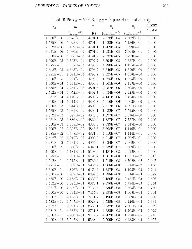
APPENDIX B. TABLES OF MODELS 203
Table B.15: Teff = 6000 K, log g = 9, pure H (non-blanketed)
τR m T Pg Pe
FconvFtotal
(g cm−2) (K) (dyn cm−2) (dyn cm−2)1.000E−06 7.375E−05 4791.1 7.378E+04 4.362E−01 0.0001.585E−06 1.023E−04 4791.0 1.023E+05 5.136E−01 0.0002.512E−06 1.409E−04 4791.1 1.409E+05 6.029E−01 0.0003.981E−06 1.930E−04 4791.4 1.931E+05 7.065E−01 0.0006.310E−06 2.636E−04 4791.9 2.637E+05 8.273E−01 0.0001.000E−05 3.593E−04 4792.7 3.594E+05 9.687E−01 0.0001.585E−05 4.888E−04 4793.9 4.890E+05 1.135E+00 0.0002.512E−05 6.643E−04 4795.2 6.646E+05 1.329E+00 0.0003.981E−05 9.021E−04 4796.7 9.025E+05 1.558E+00 0.0006.310E−05 1.224E−03 4798.3 1.225E+06 1.825E+00 0.0001.000E−04 1.661E−03 4800.0 1.661E+06 2.139E+00 0.0001.585E−04 2.251E−03 4801.5 2.252E+06 2.504E+00 0.0002.512E−04 3.052E−03 4802.7 3.054E+06 2.929E+00 0.0003.981E−04 4.140E−03 4803.7 4.141E+06 3.423E+00 0.0006.310E−04 5.614E−03 4804.8 5.616E+06 4.003E+00 0.0001.000E−03 7.614E−03 4806.5 7.617E+06 4.691E+00 0.0001.585E−03 1.032E−02 4809.1 1.032E+07 5.515E+00 0.0002.512E−03 1.397E−02 4813.3 1.397E+07 6.516E+00 0.0003.981E−03 1.886E−02 4820.0 1.887E+07 7.757E+00 0.0006.310E−03 2.538E−02 4830.3 2.539E+07 9.345E+00 0.0001.000E−02 3.397E−02 4846.3 3.398E+07 1.146E+01 0.0001.585E−02 4.508E−02 4871.3 4.510E+07 1.444E+01 0.0002.512E−02 5.912E−02 4909.0 5.914E+07 1.892E+01 0.0003.981E−02 7.631E−02 4964.6 7.634E+07 2.609E+01 0.0006.310E−02 9.636E−02 5046.1 9.639E+07 3.869E+01 0.0001.000E−01 1.181E−01 5193.9 1.181E+08 6.922E+01 0.0001.585E−01 1.361E−01 5494.2 1.361E+08 1.831E+02 0.0132.512E−01 1.515E−01 5732.6 1.515E+08 3.702E+02 0.0473.981E−01 1.667E−01 5954.9 1.668E+08 6.814E+02 0.1366.310E−01 1.826E−01 6174.3 1.827E+08 1.195E+03 0.2411.000E+00 1.997E−01 6398.6 1.998E+08 2.046E+03 0.3781.585E+00 2.185E−01 6632.2 2.186E+08 3.457E+03 0.5362.512E+00 2.395E−01 6878.1 2.396E+08 5.794E+03 0.6543.981E+00 2.629E−01 7138.5 2.630E+08 9.665E+03 0.7406.310E+00 2.894E−01 7415.6 2.895E+08 1.608E+04 0.8041.000E+01 3.195E−01 7711.7 3.196E+08 2.669E+04 0.8501.585E+01 3.537E−01 8028.2 3.539E+08 4.420E+04 0.8832.512E+01 3.931E−01 8368.1 3.932E+08 7.301E+04 0.9093.981E+01 4.383E−01 8731.8 4.385E+08 1.203E+05 0.9296.310E+01 4.900E−01 9119.2 4.902E+08 1.978E+05 0.9451.000E+02 5.507E−01 9538.0 5.509E+08 3.233E+05 0.957

APPENDIX B. TABLES OF MODELS 204
Table B.16: Teff = 8000 K, log g = 9, pure H (line-blanketed)
τR m T Pg Pe
FconvFtotal
(g cm−2) (K) (dyn cm−2) (dyn cm−2)1.000E−06 5.985E−06 6419.6 5.987E+03 1.169E+01 0.0001.585E−06 8.535E−06 6393.6 8.539E+03 1.321E+01 0.0002.512E−06 1.220E−05 6371.1 1.220E+04 1.506E+01 0.0003.981E−06 1.740E−05 6352.0 1.740E+04 1.727E+01 0.0006.310E−06 2.473E−05 6335.9 2.474E+04 1.989E+01 0.0001.000E−05 3.502E−05 6322.4 3.503E+04 2.299E+01 0.0001.585E−05 4.936E−05 6311.1 4.938E+04 2.663E+01 0.0002.512E−05 6.930E−05 6301.2 6.933E+04 3.089E+01 0.0003.981E−05 9.696E−05 6292.3 9.700E+04 3.583E+01 0.0006.310E−05 1.352E−04 6284.4 1.353E+05 4.159E+01 0.0001.000E−04 1.880E−04 6277.5 1.881E+05 4.830E+01 0.0001.585E−04 2.607E−04 6271.8 2.608E+05 5.617E+01 0.0002.512E−04 3.607E−04 6267.3 3.608E+05 6.542E+01 0.0003.981E−04 4.976E−04 6263.9 4.978E+05 7.626E+01 0.0006.310E−04 6.849E−04 6261.6 6.852E+05 8.902E+01 0.0001.000E−03 9.409E−04 6260.3 9.412E+05 1.041E+02 0.0001.585E−03 1.289E−03 6261.2 1.290E+06 1.220E+02 0.0002.512E−03 1.763E−03 6264.6 1.764E+06 1.438E+02 0.0003.981E−03 2.403E−03 6271.6 2.404E+06 1.705E+02 0.0006.310E−03 3.264E−03 6284.1 3.265E+06 2.043E+02 0.0001.000E−02 4.410E−03 6305.1 4.412E+06 2.486E+02 0.0001.585E−02 5.917E−03 6338.3 5.919E+06 3.095E+02 0.0002.512E−02 7.864E−03 6389.8 7.867E+06 3.985E+02 0.0003.981E−02 1.031E−02 6466.8 1.032E+07 5.366E+02 0.0006.310E−02 1.330E−02 6578.9 1.330E+07 7.664E+02 0.0001.000E−01 1.678E−02 6738.6 1.679E+07 1.179E+03 0.0001.585E−01 2.045E−02 7073.5 2.045E+07 2.406E+03 0.0012.512E−01 2.374E−02 7499.7 2.374E+07 5.252E+03 0.0193.981E−01 2.699E−02 7887.5 2.700E+07 1.003E+04 0.0756.310E−01 3.033E−02 8257.9 3.034E+07 1.761E+04 0.1701.000E+00 3.396E−02 8630.3 3.398E+07 2.978E+04 0.3201.585E+00 3.795E−02 9006.7 3.797E+07 4.861E+04 0.4582.512E+00 4.243E−02 9393.5 4.245E+07 7.773E+04 0.6083.981E+00 4.753E−02 9791.0 4.754E+07 1.217E+05 0.7026.310E+00 5.339E−02 10202.9 5.341E+07 1.880E+05 0.7901.000E+01 6.019E−02 10627.7 6.021E+07 2.858E+05 0.8441.585E+01 6.811E−02 11065.7 6.814E+07 4.283E+05 0.8882.512E+01 7.741E−02 11516.6 7.744E+07 6.330E+05 0.9163.981E+01 8.843E−02 11982.7 8.847E+07 9.255E+05 0.938

APPENDIX B. TABLES OF MODELS 205
Table B.17: Teff = 10000 K, log g = 9, pure H (line-blanketed)
τR m T Pg Pe
FconvFtotal
(g cm−2) (K) (dyn cm−2) (dyn cm−2)1.000E−06 1.085E−06 7747.8 1.085E+03 4.951E+01 0.0001.585E−06 1.490E−06 7762.3 1.490E+03 5.962E+01 0.0002.512E−06 2.082E−06 7756.0 2.082E+03 7.031E+01 0.0003.981E−06 2.969E−06 7733.7 2.970E+03 8.177E+01 0.0006.310E−06 4.309E−06 7704.8 4.311E+03 9.493E+01 0.0001.000E−05 6.323E−06 7676.3 6.325E+03 1.107E+02 0.0001.585E−05 9.324E−06 7647.1 9.328E+03 1.292E+02 0.0002.512E−05 1.375E−05 7621.2 1.375E+04 1.512E+02 0.0003.981E−05 2.024E−05 7592.6 2.025E+04 1.760E+02 0.0006.310E−05 2.975E−05 7562.3 2.976E+04 2.041E+02 0.0001.000E−04 4.364E−05 7533.7 4.366E+04 2.368E+02 0.0001.585E−04 6.368E−05 7513.1 6.370E+04 2.773E+02 0.0002.512E−04 9.221E−05 7501.3 9.225E+04 3.278E+02 0.0003.981E−04 1.322E−04 7500.5 1.323E+05 3.923E+02 0.0006.310E−04 1.875E−04 7511.4 1.876E+05 4.754E+02 0.0001.000E−03 2.629E−04 7532.9 2.630E+05 5.824E+02 0.0001.585E−03 3.648E−04 7563.2 3.650E+05 7.191E+02 0.0002.512E−03 5.016E−04 7597.4 5.018E+05 8.890E+02 0.0003.981E−03 6.854E−04 7630.0 6.856E+05 1.092E+03 0.0006.310E−03 9.319E−04 7670.1 9.322E+05 1.354E+03 0.0001.000E−02 1.259E−03 7725.6 1.259E+06 1.709E+03 0.0001.585E−02 1.684E−03 7805.1 1.684E+06 2.222E+03 0.0002.512E−02 2.223E−03 7911.5 2.223E+06 2.975E+03 0.0003.981E−02 2.892E−03 8044.1 2.893E+06 4.084E+03 0.0006.310E−02 3.708E−03 8213.8 3.709E+06 5.811E+03 0.0001.000E−01 4.630E−03 8554.1 4.632E+06 1.001E+04 0.0001.585E−01 5.491E−03 9065.5 5.493E+06 1.966E+04 0.0112.512E−01 6.344E−03 9521.8 6.347E+06 3.405E+04 0.0493.981E−01 7.238E−03 9959.3 7.240E+06 5.525E+04 0.1216.310E−01 8.209E−03 10390.4 8.213E+06 8.599E+04 0.2291.000E+00 9.296E−03 10814.4 9.299E+06 1.291E+05 0.3611.585E+00 1.054E−02 11233.5 1.055E+07 1.887E+05 0.5112.512E+00 1.200E−02 11645.5 1.201E+07 2.686E+05 0.6433.981E+00 1.374E−02 12059.0 1.374E+07 3.766E+05 0.7556.310E+00 1.583E−02 12476.3 1.583E+07 5.214E+05 0.8271.000E+01 1.837E−02 12902.1 1.838E+07 7.161E+05 0.8821.585E+01 2.149E−02 13340.5 2.150E+07 9.785E+05 0.9192.512E+01 2.534E−02 13793.1 2.535E+07 1.331E+06 0.9423.981E+01 3.011E−02 14262.0 3.012E+07 1.803E+06 0.9586.310E+01 3.605E−02 14750.0 3.606E+07 2.436E+06 0.9691.000E+02 4.350E−02 15260.4 4.352E+07 3.283E+06 0.977
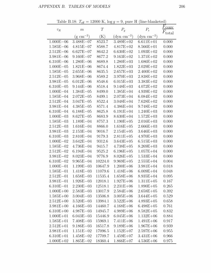
APPENDIX B. TABLES OF MODELS 206
Table B.18: Teff = 12000 K, log g = 9, pure H (line-blanketed)
τR m T Pg Pe
FconvFtotal
(g cm−2) (K) (dyn cm−2) (dyn cm−2)1.000E−06 3.488E−07 8523.7 3.489E+02 6.611E+01 0.0001.585E−06 4.815E−07 8588.7 4.817E+02 8.566E+01 0.0002.512E−06 6.627E−07 8642.2 6.630E+02 1.093E+02 0.0003.981E−06 9.160E−07 8677.2 9.163E+02 1.371E+02 0.0006.310E−06 1.280E−06 8689.8 1.280E+03 1.686E+02 0.0001.000E−05 1.821E−06 8674.4 1.822E+03 2.029E+02 0.0001.585E−05 2.655E−06 8635.5 2.657E+03 2.400E+02 0.0002.512E−05 3.968E−06 8589.2 3.970E+03 2.838E+02 0.0003.981E−05 6.012E−06 8548.6 6.015E+03 3.383E+02 0.0006.310E−05 9.144E−06 8518.4 9.148E+03 4.072E+02 0.0001.000E−04 1.384E−05 8499.0 1.385E+04 4.939E+02 0.0001.585E−04 2.072E−05 8499.1 2.073E+04 6.084E+02 0.0002.512E−04 3.047E−05 8522.4 3.048E+04 7.628E+02 0.0003.981E−04 4.385E−05 8571.4 4.386E+04 9.748E+02 0.0006.310E−04 6.188E−05 8625.8 6.191E+04 1.240E+03 0.0001.000E−03 8.627E−05 8683.9 8.630E+04 1.572E+03 0.0001.585E−03 1.189E−04 8757.3 1.190E+05 2.016E+03 0.0002.512E−03 1.616E−04 8866.0 1.616E+05 2.666E+03 0.0003.981E−03 2.153E−04 9016.7 2.154E+05 3.646E+03 0.0006.310E−03 2.810E−04 9179.3 2.811E+05 4.970E+03 0.0001.000E−02 3.642E−04 9312.6 3.643E+05 6.515E+03 0.0001.585E−02 4.736E−04 9415.7 4.738E+05 8.269E+03 0.0002.512E−02 6.194E−04 9525.2 6.196E+05 1.057E+04 0.0003.981E−02 8.023E−04 9776.9 8.026E+05 1.533E+04 0.0006.310E−02 9.965E−04 10224.0 9.969E+05 2.555E+04 0.0041.000E−01 1.199E−03 10647.9 1.200E+06 3.981E+04 0.0181.585E−01 1.418E−03 11079.6 1.418E+06 6.009E+04 0.0482.512E−01 1.658E−03 11535.4 1.658E+06 8.935E+04 0.0953.981E−01 1.926E−03 12018.1 1.927E+06 1.311E+05 0.1676.310E−01 2.230E−03 12518.1 2.231E+06 1.890E+05 0.2651.000E+00 2.583E−03 13017.9 2.584E+06 2.658E+05 0.3921.585E+00 3.004E−03 13506.8 3.005E+06 3.644E+05 0.5292.512E+00 3.520E−03 13984.1 3.522E+06 4.893E+05 0.6583.981E+00 4.166E−03 14460.7 4.168E+06 6.498E+05 0.7616.310E+00 4.987E−03 14945.7 4.989E+06 8.582E+05 0.8321.000E+01 6.043E−03 15446.9 6.045E+06 1.132E+06 0.8841.585E+01 7.408E−03 15969.1 7.411E+06 1.491E+06 0.9172.512E+01 9.186E−03 16517.8 9.189E+06 1.967E+06 0.9393.981E+01 1.151E−02 17096.5 1.152E+07 2.597E+06 0.9556.310E+01 1.458E−02 17709.7 1.459E+07 3.431E+06 0.9661.000E+02 1.865E−02 18360.4 1.866E+07 4.536E+06 0.975

Appendix C
Southern Spectropolarimetric
Survey
A summarized observation log of white dwarfs using the Steward Observatory CCD
Spectropolarimeter attached to the 74 inch telescope at MSO is given in Table C.1.
The first column gives the WD number, the second column gives an alternate name,
the third column gives the date that the object was observed and the fourth column
gives the number of exposures taken for that night and the length of one exposure,
that is the time it takes for one waveplate sequence to be completed. The table
also gives the measured longitudinal magnetic field for each spectrum at Hα, Hβ,
Hγ, and also the weighted average of these three measurements. These values are
presented in final four columns. Figures C.1 to C.10 show the flux and polarization
spectra of white dwarfs listed in Table C.1 (excluding the spectra that was shown
in the text).
The summarized observation log of the complementary spectroscopic observa-
tions is presented in Table C.2. In this table, the WD number and an alternate
name are given in columns 1 and two, respectively. The UT date of the observa-
tion in column 3, the number of exposures for that given date in column 4 and the
exposure time in column 5. The spectra of these observations are shown in Fig-
207
APPENDIX C. SOUTHERN SPECTROPOLARIMETRIC SURVEY 208
ures C.11 to C.14. The spectra are shown in order of increasing temperature with
WD 0141−675 being the coolest. The figures also show the spectra of three sdB
stars (GD 687, BPM 36430 and GD 108) that have been observed, and two WD
plus dMe binary systems (WD 0718−316 and WD 0419−487).

APPENDIX C. SOUTHERN SPECTROPOLARIMETRIC SURVEY 209
Tab
leC
.1:
Obse
rvat
ion
log
ofw
hit
edw
arfs
inth
eso
uth
ern
spec
trop
olar
imet
ric
surv
eyW
DO
ther
Nam
eD
ate
Exp
.tim
eB
(kG
)(s
)H
αH
βH
γW
eigh
ted
Ave
rage
0018−3
39G
D60
325
/11/
2000
4×
400
−21.
5±
18.5
−15.
8±
13.5
39.0
±16
.00.
23±
9.01
02/1
2/20
002×
720
3.1±
26.0
21.1
±14
.047
.9±
25.6
22.8
6±
11.1
104
/12/
2000
3×
720
1.5±
11.4
−11.
2±
13.8
−16.
6±
23.8
−5.2
1±
8.24
0047−5
24B
PM
1627
401
/12/
2000
3×
720
−28.
8±
17.8
−10.
2±
12.1
7.9±
18.2
−10.
51±
8.77
0050−3
32G
D65
925
/12/
2000
3×
480
8.5±
11.2
−15.
1±
8.7
32.3
±16
.1−0
.28±
6.32
0106−3
58G
D68
301
/12/
2000
3×
720
−14.
0±
23.3
−1.1
±15
.845
.5±
29.9
2.97
±11
.98
24/1
2/20
002×
720
2.5±
12.6
−6.5
±12
.6−2
.7±
17.1
−2.1
5±
7.90
0107−3
42G
D68
701
/12/
2000
2×
720
17.5
±21
.8−2
7.4±
9.8
−5.7
±20
.4−1
7.57
±8.
1924
/12/
2000
3×
600
−4.3
±5.
9−7
.5±
6.0
−2.0
±8.
9−5
.17±
3.80
0126−5
32B
PM
1650
105
/11/
2000
1×
800
34.6
±19
.33.
9±
16.7
−8.8
±27
.912
.65±
11.5
026
/11/
2000
3×
720
−1.6
±9.
95.
3±
9.3
16.0
±8.
97.
18±
5.39
0131−1
64G
D98
426
/12/
2000
4×
720
34.0
±12
.24.
6±
13.6
35.3
±20
.423
.27±
8.30
0141−6
75LT
T93
427
/10/
2000
2×
2400
0.5±
4.1
10.7
±8.
518
.7±
20.6
2.93
±3.
6303
/11/
2000
3×
800
0.7±
4.2
−2.9
±4.
7−3
4.6±
20.3
−1.6
8±
3.10
0255−7
05LH
S14
7428
/10/
2000
3×
1200
0.1±
5.9
5.6±
5.1
−21.
8±
10.5
0.27
±3.
6203
10−6
88LB
3303
28/1
0/20
003×
720
−9.2
±3.
3−6
.7±
1.8
3.1±
4.4
−6.0
9±
1.49
0325−8
57LB
9802
23/1
2/20
005×
720
6.8±
6.2
−2.9
±8.
117
.3±
7.9
7.16
±4.
1803
41−4
59B
PM
3159
425
/11/
2000
4×
600
5.5±
12.4
12.4
±7.
411
.2±
11.7
10.7
3±
5.58
26/1
1/20
003×
600
3.8±
16.8
−17.
6±
12.9
55.6
±19
.74.
20±
9.08
0419−4
87LT
T19
5126
/11/
2000
4×
600
−2.2
±6.
429
.1±
24.7
−0.2
3±
6.20
Con
tinu
eson
next
page

APPENDIX C. SOUTHERN SPECTROPOLARIMETRIC SURVEY 210
Tab
leC
.1–
cont
inue
dfr
ompr
evio
uspa
geW
DO
ther
Nam
eD
ate
Exp
.tim
eB
(kG
)(s
)H
αH
βH
γW
eigh
ted
Ave
rage
24/1
2/20
0019
.6±
42.2
−6.0
±36
.85.
06±
27.7
426
/12/
2000
3×
720
−35.
1±
22.2
14.6
±10
.16.
08±
9.19
18/0
1/20
013×
480
−3.4
±22
.1−6
2.4±
32.1
17.7
6±
18.2
004
46−7
89B
PM
3523
03/1
1/20
002×
600
1.7±
8.9
−13.
4±
8.4
−15.
3±
14.0
−7.7
3±
5.60
24/1
2/20
003×
600
−1.1
±10
.10.
1±
6.9
−19.
2±
5.2
−10.
60±
3.84
0455−2
82M
CT
0455−2
812
26/1
2/20
003×
720
−9.1
±18
.411
.0±
16.0
16.1
±21
.85.
57±
10.5
605
09−0
07E
UV
EJ0
512−
006
25/1
2/20
003×
480
23.5
±11
.2−1
.3±
9.5
−3.1
±15
.06.
77±
6.52
0549
+15
8G
D71
26/1
2/20
003×
480
1.6±
10.2
25.5
±8.
5−2
1.8±
17.5
11.1
2±
6.12
0621−3
76E
UV
EJ0
623−
376
02/1
2/20
004×
240
−10.
7±
12.8
−11.
3±
8.9
−11.
2±
17.5
−11.
12±
6.74
0646−2
53E
UV
EJ0
648−
253
26/1
2/20
002×
480
3.3±
8.2
6.3±
5.9
14.3
±11
.56.
61±
4.42
0652−5
63E
UV
EJ0
653−
564
21/0
2/20
014×
720
76.7
±80
.5−5
.7±
53.6
−95.
4±
86.5
−4.5
6±
39.6
507
01−5
87B
PM
1839
425
/11/
2000
4×
600
5.9±
9.0
2.7±
6.7
−27.
7±
14.0
−0.2
1±
5.02
24/1
2/20
003×
720
−27.
6±
12.9
7.8±
9.4
−23.
7±
14.9
−8.4
4±
6.77
0715−7
03E
UV
EJ0
715−
704
28/1
2/20
004×
720
−32.
2±
24.2
23.1
±16
.2−3
0.5±
25.1
−2.1
6±
11.8
631
/12/
2000
3×
720
−22.
2±
30.4
−49.
2±
19.6
−52.
1±
31.1
−43.
64±
14.5
601
/01/
2001
7×
720
1.7±
10.1
−12.
0±
8.2
−8.1
±9.
1−7
.06±
5.22
17/0
2/20
013×
720
−14.
8±
15.2
−16.
8±
9.5
8.3±
17.3
−11.
87±
7.30
0718−3
16E
UV
EJ0
720−
317
02/1
2/20
005×
720
53.1
±35
.049
.2±
36.1
51.2
1±
25.1
307
21−2
76E
UV
EJ0
723−
277
28/1
2/20
005×
720
−28.
3±
14.8
−11.
2±
11.7
29.0
±20
.7−1
0.09
±8.
3907
32−4
27B
PM
3303
927
/12/
2000
3×
720
−2.5
±10
.2−0
.9±
8.2
3.8±
7.5
0.71
±4.
8621
/02/
2001
3×
480
−10.
1±
8.9
11.8
±8.
216
.5±
8.8
6.46
±4.
9707
40−5
70B
PM
1861
527
/12/
2000
5×
720
−2.4
±15
.6−1
0.0±
13.2
0.0±
20.3
−5.4
8±
9.03
0821−2
52E
UV
EJ0
823−
254
04/1
2/20
009×
720
−137
.9±
87.1
−644
.0±
116.
9−5
36.5
±89
.7−5
76.3
4±
71.1
6a
Con
tinu
eson
next
page
aH
αm
easu
rem
ent
was
excl
uded
inth
eca
lcul
atio
nof
the
mea
n,se
ete
xtfo
rde
tails

APPENDIX C. SOUTHERN SPECTROPOLARIMETRIC SURVEY 211
Tab
leC
.1–
cont
inue
dfr
ompr
evio
uspa
geW
DO
ther
Nam
eD
ate
Exp
.tim
eB
(kG
)(s
)H
αH
βH
γW
eigh
ted
Ave
rage
01/0
1/20
016×
720
−74.
3±
112.
8−5
91.1
±12
0.2
−836
.1±
135.
7−6
98.8
1±
89.9
8a
25/0
2/20
015×
720
22.7
±39
.5−5
83.2
±13
0.5
−465
.0±
166.
4−5
38.1
9±
102.
69a
0839−3
27LFT
600
25/1
1/20
003×
240
5.2±
2.4
3.2±
3.5
−7.8
±5.
02.
89±
1.84
0850−6
17B
PM
5109
25/1
1/20
002×
720
0.3±
18.2
18.1
±11
.9−1
5.5±
15.6
4.58
±8.
3926
/11/
2000
3×
720
21.0
±13
.213
.7±
13.3
25.1
±22
.418
.53±
8.64
0859−0
39E
UV
EJ0
902−
041
23/1
2/20
001×
600
−10.
5±
8.5
−15.
7±
8.4
34.8
±20
.6−9
.41±
5.74
26/1
2/20
003×
480
5.7±
7.9
10.7
±9.
70.
6±
10.8
5.97
±5.
3309
50−5
72B
PM
1973
804
/12/
2000
3×
720
12.5
±9.
7−5
.6±
8.2
−2.1
±13
.81.
25±
5.70
24/1
2/20
003×
720
−2.5
±9.
912
.0±
11.7
−11.
7±
17.0
1.03
±6.
9109
54−7
10B
PM
6082
02/1
2/20
005×
480
−0.1
±4.
6−0
.8±
4.7
1.5±
6.0
0.01
±2.
8809
57−6
66B
PM
6114
01/1
2/20
002×
720
−23.
0±
16.5
−8.5
±14
.58.
1±
20.4
−9.7
3±
9.61
0958−0
73G
D10
827
/12/
2000
1×
720
−6.7
±10
.5−2
4.2±
8.3
33.2
±20
.80.
01±
2.88
1013−0
50E
UV
EJ1
016−
053
25/0
2/20
015×
720
−18.
7±
23.3
−15.
4±
23.3
−18.
31±
21.8
710
22−3
01E
UV
EJ1
024−
303
21/0
2/20
016×
720
12.0
±36
.5−1
2.4±
22.9
1.7±
48.9
−4.5
3±
18.0
310
42−6
90B
PM
6502
23/1
2/20
002×
600
−35.
9±
12.0
−11.
7±
7.7
−29.
9±
15.3
−20.
45±
5.97
1053−5
50LT
T40
1319
/01/
2001
5×
480
6.3±
7.5
−10.
5±
7.7
−16.
4±
14.0
−3.7
4±
5.02
20/0
1/20
013×
480
−19.
7±
9.9
0.3±
10.3
−18.
0±
11.9
−12.
19±
6.12
27/0
1/20
014×
600
0.8±
9.9
9.8±
7.7
−17.
4±
12.0
1.55
±5.
4210
56−3
84E
UV
EJ1
058−
387
01/0
1/20
016×
720
7.0±
5.0
2.7±
6.1
7.9±
6.9
5.90
±3.
3711
21−5
07B
PM
2091
217
/02/
2001
3×
720
23.9
±9.
2−1
2.7±
6.6
−2.0
±14
.5−0
.47±
5.03
18/0
2/20
013×
720
−12.
2±
7.3
−2.8
±9.
210
.3±
14.5
−6.0
3±
5.32
1153−4
84B
PM
3643
019
/01/
2001
2×
240
−10.
3±
8.5
−16.
0±
7.8
5.1±
13.1
−10.
41±
5.26
20/0
1/20
014×
240
3.2±
3.5
2.5±
4.2
−0.5
±8.
62.
61±
2.57
1236−4
95LT
T48
1620
/01/
2001
5×
360
−4.2
±5.
22.
3±
7.9
−6.3
±14
.2−2
.58±
4.15
Con
tinu
eson
next
page

APPENDIX C. SOUTHERN SPECTROPOLARIMETRIC SURVEY 212
Tab
leC
.1–
cont
inue
dfr
ompr
evio
uspa
geW
DO
ther
Nam
eD
ate
Exp
.tim
eB
(kG
)(s
)H
αH
βH
γW
eigh
ted
Ave
rage
1257−7
23B
PM
7961
21/0
2/20
014×
720
−2.7
±12
.0−0
.5±
6.7
−41.
7±
13.1
−7.7
9±
5.34
1323−5
14LFT
1004
17/0
2/20
013×
720
7.1±
11.0
−5.9
±8.
1−3
.0±
9.9
−1.8
4±
5.45
18/0
2/20
013×
720
−0.3
±10
.41.
0±
8.8
−11.
6±
12.5
−2.2
4±
5.92
1407−4
75B
PM
3816
517
/02/
2001
3×
720
15.1
±8.
09.
8±
8.4
17.7
±13
.913
.34±
5.35
1425−8
11B
PM
784
18/0
2/20
014×
480
−4.1
±5.
38.
2±
5.9
6.9±
6.9
2.75
±3.
4215
29−7
72E
UV
EJ1
535−
774
25/0
2/20
015×
720
87.6
±11
2.3
85.6
±18
3.1
87.0
5±
95.7
315
44−3
77LT
T63
0218
/02/
2001
3×
480
−7.9
±7.
0−1
.7±
8.8
−8.5
±14
.3−5
.88±
5.12
21/0
2/20
012×
480
−10.
2±
7.9
2.1±
6.0
9.0±
9.9
−0.2
5±
4.30
1616−5
91B
PM
2404
721
/02/
2001
2×
720
17.6
±8.
73.
7±
9.4
−18.
9±
16.5
7.27
±5.
9522
/02/
2001
2×
720
−13.
0±
9.5
−2.3
±11
.8−8
.1±
15.0
−8.6
6±
6.64
1620−3
91C
D−3
810
980
21/0
2/20
013×
240
−2.7
±2.
6−3
.2±
2.7
−3.1
±4.
6−2
.96±
1.73
1628−8
73B
PM
890
22/0
2/20
014×
720
−0.5
±6.
118
.0±
6.8
5.9±
10.4
7.45
±4.
1616
59−5
31B
PM
2460
121
/02/
2001
2×
480
−0.1
±7.
7−1
.2±
5.4
−1.7
±7.
4−1
.06±
3.80
1724−3
59E
UV
EJ1
727−
360
25/0
2/20
013×
720
−15.
9±
32.9
23.6
±21
.711
.6±
43.3
11.6
2±
16.7
120
07−3
03LT
T79
8727
/10/
2000
1×
1200
0.2±
7.1
3.8±
11.6
21.6
±11
.75.
50±
5.38
29/1
0/20
002×
1200
6.9±
3.5
−4.8
±4.
96.
3±
5.4
3.68
±2.
5220
39−6
82LT
T81
9005
/11/
2000
2×
800
−18.
8±
8.4
0.6±
5.6
−9.3
±10
.7−6
.00±
4.27
2105−8
20B
PM
1266
28/1
0/20
003×
1200
2.1±
4.7
1.5±
5.8
10.7
±8.
03.
39±
3.32
2115−5
60LT
T84
5205
/11/
2000
3×
800
−5.2
±7.
2−1
.7±
7.5
8.4±
11.1
−1.3
8±
4.70
2159−7
54LT
T88
1625
/11/
2000
4×
800
−6.0
±9.
1−9
.9±
7.7
0.3±
23.1
−7.7
5±
5.70
02/1
2/20
003×
720
−20.
7±
7.0
−4.8
±6.
85.
9±
24.9
−11.
84±
4.79
2211−4
95E
UV
EJ2
214−
493
02/1
2/20
005×
480
12.7
±5.
0−2
.3±
5.9
7.5±
9.8
6.57
±3.
5522
32−5
75LT
T90
8204
/12/
2000
5×
720
19.7
±12
.71.
0±
8.7
48.7
±20
.611
.49±
6.78
2329−2
91G
D16
6924
/12/
2000
3×
600
−2.7
±7.
41.
4±
4.9
0.5±
12.1
0.19
±3.
87C
ontinu
eson
next
page

APPENDIX C. SOUTHERN SPECTROPOLARIMETRIC SURVEY 213
Tab
leC
.1–
cont
inue
dfr
ompr
evio
uspa
geW
DO
ther
Nam
eD
ate
Exp
.tim
eB
(kG
)(s
)H
αH
βH
γW
eigh
ted
Ave
rage
25/1
2/20
003×
600
10.8
±5.
81.
5±
8.9
1.4±
11.8
7.07
±4.
4923
31−4
75E
UV
EJ2
334−
472
25/1
2/20
003×
600
−2.1
±15
.916
.6±
22.0
−22.
7±
22.9
−2.1
8±
11.2
323
37−7
60LT
T96
4803
/12/
2000
2×
720
−12.
7±
37.5
12.1
±16
.224
.6±
29.9
11.4
5±
13.3
204
/12/
2000
6×
480
24.8
±17
.56.
4±
8.5
15.1
±13
.411
.19±
6.64
2359−4
34LT
T98
5727
/10/
2000
2×
1200
5.9±
3.9
−3.1
±5.
47.
4±
8.2
3.41
±2.
95

APPENDIX C. SOUTHERN SPECTROPOLARIMETRIC SURVEY 214
Figure C.1: Flux and polarization spectra.

APPENDIX C. SOUTHERN SPECTROPOLARIMETRIC SURVEY 215
Figure C.2: Flux and polarization spectra.

APPENDIX C. SOUTHERN SPECTROPOLARIMETRIC SURVEY 216
Figure C.3: Flux and polarization spectra.

APPENDIX C. SOUTHERN SPECTROPOLARIMETRIC SURVEY 217
Figure C.4: Flux and polarization spectra.
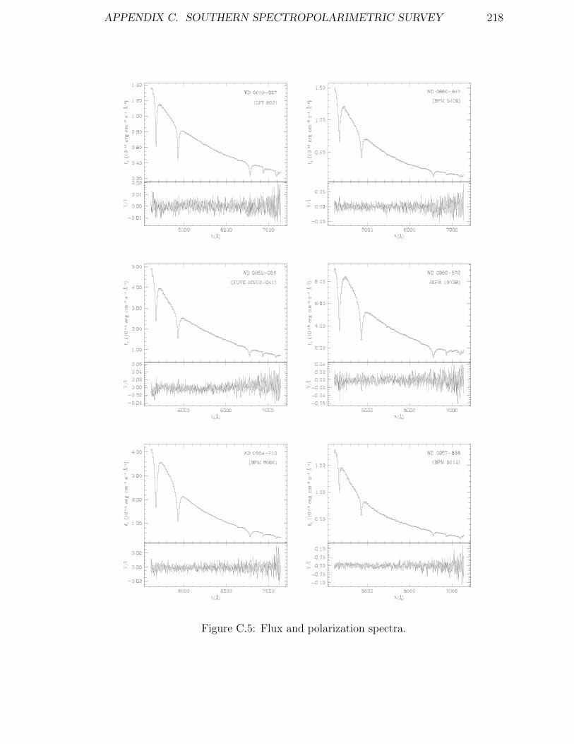
APPENDIX C. SOUTHERN SPECTROPOLARIMETRIC SURVEY 218
Figure C.5: Flux and polarization spectra.
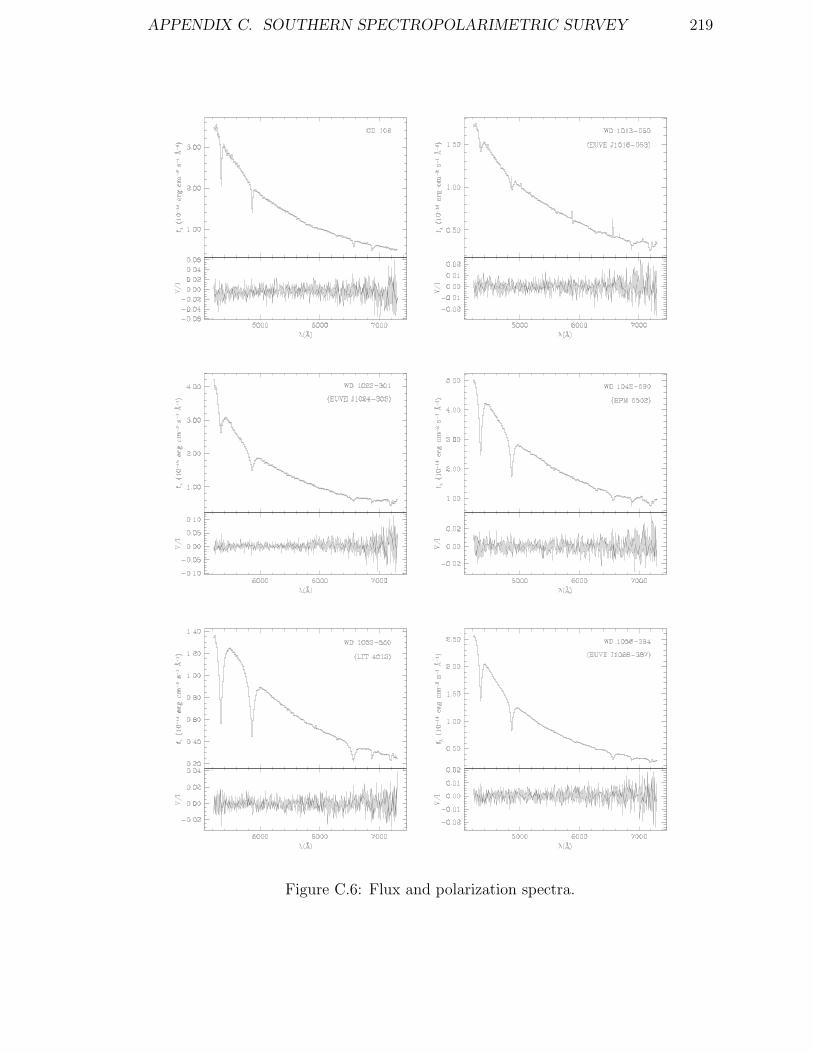
APPENDIX C. SOUTHERN SPECTROPOLARIMETRIC SURVEY 219
Figure C.6: Flux and polarization spectra.

APPENDIX C. SOUTHERN SPECTROPOLARIMETRIC SURVEY 220
Figure C.7: Flux and polarization spectra.

APPENDIX C. SOUTHERN SPECTROPOLARIMETRIC SURVEY 221
Figure C.8: Flux and polarization spectra.

APPENDIX C. SOUTHERN SPECTROPOLARIMETRIC SURVEY 222
Figure C.9: Flux and polarization spectra.

APPENDIX C. SOUTHERN SPECTROPOLARIMETRIC SURVEY 223
Figure C.10: Flux and polarization spectra.

APPENDIX C. SOUTHERN SPECTROPOLARIMETRIC SURVEY 224
Table C.2: Observation log of complementary spectroscopy of white dwarfs in thesouthern spectropolarimetric survey
WD Other Name Date Number Exp. time (s)0018−339 BPM 46232 25/10/2001 2 18000047−524 BPM 16274 25/10/2001 2 18000107−342 GD 687 25/10/2001 1 18000126−532 BPM 16501 25/10/2001 2 18000141−675 LTT 934 04/03/2001 4 600
28/10/2001 4 18000255−705 LHS 1474 28/02/2001 3 9000310−688 EG 21 08/03/2002 3 300
08/01/2002 1 9000341−459 BPM 31594 02/03/2001 3 9000419−487 LTT 1951 04/03/2001 4 9000701−587 BPM 18394 04/03/2001 2 9000718−316 EUVE J0720−317 07/01/2002 3 18000732−427 BPM 33039 04/03/2001 2 9000740−570 BPM 18615 05/03/2001 3 9000800−533 BPM 18764 07/01/2002 3 1800
08/01/2002 2 24000839−327 LFT 600 02/03/2001 3 3000850−617 BPM 5109 25/10/2001 1 1800
28/10/2001 2 180008/01/2002 3 1800
0950−572 BPM 19738 02/03/2001 3 9000954−710 BPM 6082 02/03/2001 3 6000958−073 GD 108 07/03/2001 3 600
08/01/2002 1 9001053−550 LTT 4013 04/03/2001 2 9001121−507 BPM 20912 07/03/2001 3 9001153−484 BPM 36430 07/01/2002 3 12001223−688 BPM 7543 08/03/2001 4 6001236−495 LTT 4816 02/03/2001 3 9001257−723 BPM 7961 07/01/2002 3 1800
07/01/2002 1 12001323−514 BPM 21970 08/01/2002 2 18001407−475 BPM 38165 08/01/2002 2 18001425−811 BPM 784 02/03/2001 3 6001544−377 LTT 6302 02/03/2001 3 6001616−591 BPM 24047 02/03/2001 3 9001628−873 BPM 890 02/03/2001 3 9001659−531 BPM 24601 02/03/2001 3 6001709−575 LTT 6859 16/09/2001 2 1800
Continues on next page

APPENDIX C. SOUTHERN SPECTROPOLARIMETRIC SURVEY 225
Table C.2 – continued from previous pageWD Other Name Date Number Exp. time (s)
1953−715 LTT 7875 16/09/2001 3 18002007−303 LTT 7987 15/09/2001 2 9002039−682 LTT 8190 15/09/2001 3 9002105−820 LTT 8381 15/09/2001 4 9002115−560 LTT 8452 16/09/2001 2 18002159−754 LTT 8816 15/09/2001 3 1800
27/10/2001 4 18002232−560 LTT 9082 16/09/2001 2 18002337−760 BPM 15727 25/10/2001 2 1800
26/10/2001 2 18002351−368 LTT 9774 15/09/2001 2 18002359−434 LTT 9857 13/09/2001 2 600
27/10/2001 3 1800

APPENDIX C. SOUTHERN SPECTROPOLARIMETRIC SURVEY 226
Figure C.11: Spectra of white dwarfs complementary to SPOL observations with
Teff < 11500 K are shown in order of increasing temperature, from top to bottom.

APPENDIX C. SOUTHERN SPECTROPOLARIMETRIC SURVEY 227
Figure C.12: Spectra of white dwarfs complementary to SPOL observations with
11500 < Teff < 15500 K are shown in order of increasing temperature, from top
to bottom.

APPENDIX C. SOUTHERN SPECTROPOLARIMETRIC SURVEY 228
Figure C.13: Spectra of white dwarfs complementary to SPOL observations with
15500 < Teff < 19000 K are shown in order of increasing temperature, from top
to bottom.

APPENDIX C. SOUTHERN SPECTROPOLARIMETRIC SURVEY 229
Figure C.14: Spectra of white dwarfs complementary to SPOL observations with
Teff > 19000 K are shown in order of increasing temperature, from top to bottom.
Also are shown three sdB stars that have been observed along with two close WD
plus dMe binaries (WD 0718−316 and WD 0419−487).

Appendix D
Spectroscopy of Local White
Dwarfs
A summarized log of observations of NLTT candidate stars and local white dwarfs
is presented in Table D.1. In this table, the name of the star is given in column 1,
the UT date that the object was observed in column 2 and the number of exposures
taken for that night in column 3. The exposure time is given in column 4 and the
place of observation is given in column 5. Observations were carried out on the
74 inch telescope at Mount Stromlo Observatory (MSO), 2.3 m telescope at Siding
Spring Observatory (SSO) and 2.4 m telescope at MDM Observatory (MDM).
230

APPENDIX D. SPECTROSCOPY OF LOCAL WHITE DWARFS 231
Table D.1: Observations of NLTT white dwarf candidates, and other local stars
Name Date (UT) Number Exp. Time (s) Where
NLTT 529 22/06/03 1 371 MDM
23/06/03 2 360 MDM
NLTT 4828 12/09/02 1 1800 MSOa
NLTT 8435 12/09/02 2 3600 MSOa
13/09/02 1 1800 MSOa
14/09/02 3 1800 MSO
17/10/02 7 1800 MSO
18/10/02 1 1800 MSO
05/12/02 4 1800 MSO
05/12/02 1 3600 MSO
06/12/02 3 2700 MSO
07/12/02 3 2700 MSO
08/12/02 3 2700 MSO
16/12/02 1 630 SSO
16/12/02 6 1800 SSO
NLTT 8581 13/09/02 1 1800 MSOa
19/10/02 2 1800 MSO
06/12/02 5 1800 MSO
07/12/02 2 1800 MSO
NLTT 15314 13/09/02 1 900 MSOa
NLTT 19138 16/12/02 3 600 MDM
NLTT 21351 06/12/02 2 600 MSOb
NLTT 23235 17/10/02 3 1800 MSO
NLTT 24703 12/12/02 3 600 MSOd
NLTT 26398 05/12/02 1 1800 MSO
Continues on next page

APPENDIX D. SPECTROSCOPY OF LOCAL WHITE DWARFS 232
Table D.1 – continued from previous page
WD Date (UT) Number Exp. Time (s) Where
07/12/02 1 900 MSO
07/12/02 1 600 MSOc
NLTT 31748 05/12/02 1 600 MSO
06/12/02 2 900 MSO
07/12/02 1 1800 MSO
08/12/02 1 1800 MSO
11/12/02 1 1800 MSO
16/12/02 1 1500 SSO
16/12/02 1 2400 SSO
NLTT 40607 03/02/03 1 600 MDM
03/02/03 1 347 MDM
29/06/03 3 1200 SSO
NLTT 44850 14/09/02 1 900 MSO
NLTT 46292 14/09/02 1 1200 MSO
NLTT 47373 14/09/02 1 1800 MSO
14/09/02 1 900 MSO
15/09/02 6 1800 MSO
18/10/02 2 1800 MSO
19/10/02 1 3600 MSO
20/10/02 1 3600 MSO
23/10/02 1 1800 MSO
NLTT 47807 13/09/02 1 1200 MSOa
NLTT 49985 29/06/03 2 1800 SSO
NLTT 52404 29/06/03 1 1800 SSO
NLTT 52890 15/09/02 1 1800 MSO
NLTT 53177 13/09/02 2 1800 MSOa
14/09/02 3 1800 MSO
07/12/02 2 1800 MSO
Continues on next page
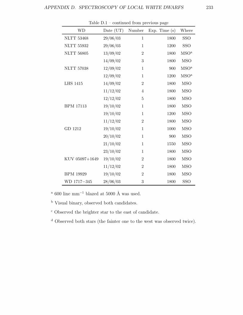
APPENDIX D. SPECTROSCOPY OF LOCAL WHITE DWARFS 233
Table D.1 – continued from previous page
WD Date (UT) Number Exp. Time (s) Where
NLTT 53468 29/06/03 1 1800 SSO
NLTT 55932 29/06/03 1 1200 SSO
NLTT 56805 13/09/02 2 1800 MSOa
14/09/02 3 1800 MSO
NLTT 57038 12/09/02 1 900 MSOa
12/09/02 1 1200 MSOa
LHS 1415 14/09/02 2 1800 MSO
11/12/02 4 1800 MSO
12/12/02 5 1800 MSO
BPM 17113 19/10/02 1 1800 MSO
19/10/02 1 1200 MSO
11/12/02 2 1800 MSO
GD 1212 19/10/02 1 1000 MSO
20/10/02 1 900 MSO
21/10/02 1 1550 MSO
23/10/02 1 1800 MSO
KUV 05097+1649 19/10/02 2 1800 MSO
11/12/02 2 1800 MSO
BPM 19929 19/10/02 2 1800 MSO
WD 1717−345 28/06/03 3 1800 SSO
a 600 line mm−1 blazed at 5000 A was used.
b Visual binary, observed both candidates.
c Observed the brighter star to the east of candidate.
d Observed both stars (the fainter one to the west was observed twice).

Appendix E
Observations of Close Binary
Systems
Figure E.1 shows the charts of four close binary systems that were observed as part
of this thesis. The charts are all 5′ × 5′ and the close binary systems are clearly
marked by the line intersects. The charts also show the reference stars used in the
reduction of the images. The charts are all second generation DSS images in R,
except for BPM 6502 which is one of the images obtained Perth Observatory using
the R filter.
Tables E.1 and E.3 list the Hα radial velocity measurements of the close binary
systems, BPM 71214 and EC 13471−1258, respectively. The tables give the Helio-
centric Julian Date (HJD) and the radial velocity measurements. Table E.2 lists the
absorption radial velocity measurements BPM 71214, where GL 190 was used as a
template star. The table gives the HJD and the radial velocity measurements. Table
E.4 lists the absorption radial velocity measurements for EC 13471−1258, where the
absorption features of EC 13471−1258 were compared to two template stars, GL
250B (column 2) and GL 190 (column 3). Tables E.5 and E.6 list the HJD, radial ve-
locity measurements and the equivalent width measurements for EUVE J0720−31.7
and BPM 6502, respectively.
234

APPENDIX E. OBSERVATIONS OF CLOSE BINARY SYSTEMS 235
Relative photometric measurements of BPM 71214, EC 13471−1258 and BPM 6502
are presented. Tables E.7 and E.8 present the photometry of BPM 71214 in the R
and I band respectively. Tables E.9 and E.10 present the photometry of EC 13471−1258
in the B and R band, respectively. Tables E.11 and E.12 present the photometry
of BPM 6502 in the R and I band, respectively. In each table, the HJD and the
photometric measurement relative to an average of the measurements for each star
and colour band.

APPENDIX E. OBSERVATIONS OF CLOSE BINARY SYSTEMS 236
Figure E.1: Charts of the close binary stars BPM 71214 (top left), EUVE J0720−317
(top right), BPM 6502 (bottom left) and EC 13471−1258 (bottom right). The close
binary systems are marked by the line intersects. The stars marked with circles and
labeled by numbers are reference stars used in the reduction of photometric images.

APPENDIX E. OBSERVATIONS OF CLOSE BINARY SYSTEMS 237
Table E.1: Hα radial velocity measurements for BPM 71214HJD (2450000+) V (km s−1) HJD (2450000+) V (km s−1)
2317.925971 149.377 2341.915241 119.6872317.939419 175.852 2341.925351 146.6292317.951871 179.943 2341.934094 168.0882317.964359 163.925 2341.943017 167.1652317.977633 136.496 2341.952368 166.2412318.014806 -6.981 2341.961280 149.7962318.028230 -41.251 2341.970168 129.6872318.041424 -69.126 2341.980919 95.4262318.051944 -60.000 2343.887207 -21.4332318.956608 167.639 2343.899440 14.6452318.972811 164.412 2343.911846 51.1692318.985495 142.018 2343.921498 86.7902319.998020 123.776 2343.934923 132.4612320.010392 84.481 2343.951693 154.8242320.022983 27.827 2364.865413 -3.673*2320.035355 -14.666 2364.876663 29.664*2334.901317 150.770 2364.887878 47.936*2334.913572 101.415 2364.900562 80.360*2334.927715 84.950 2365.868576 -76.402*2334.946915 16.866 2365.880763 10.838*2334.957573 -21.059 2365.892383 39.150*2334.966624 -46.650 2533.107869 151.5632334.975604 -72.241 2533.116874 117.2922334.984817 -99.649 2533.125810 81.6422334.993670 -100.573 2533.134607 60.1522335.002477 -55.806 2533.143461 27.2522335.910990 133.572 2533.152548 -3.3742335.924114 98.378 2533.161368 -26.2352335.936671 71.873 2533.170176 -47.2682335.949089 26.172 2533.179043 -60.5352335.961298 -13.580 2533.187874 -70.6052338.948822 145.969 2533.196810 -65.6102338.984097 0.684 2533.205665 -40.5062340.894593 79.755 2533.214566 -24.9942340.906918 124.045 2533.223421 1.0242340.919324 154.184 2533.232368 32.9702340.931789 166.955 2533.241258 66.2972340.944149 169.686 2533.250089 93.6852340.956532 140.440 2533.259048 128.3732340.967654 131.294 2533.267857 147.0822341.890683 34.751 2533.276827 166.7042341.902985 77.224 2533.289514 181.282

APPENDIX E. OBSERVATIONS OF CLOSE BINARY SYSTEMS 238
Table E.2: Absorption radial velocity measurements for BPM 71214HJD (2450000+) V (km s−1) HJD (2450000+) V (km s−1)
2317.925971 124.9 ± 21.6 2341.943017 183.2 ± 44.12317.939419 168.7 ± 18.8 2341.952368 153.0 ± 22.52317.951871 178.9 ± 20.9 2341.961280 126.7 ± 15.32317.964359 158.4 ± 19.0 2341.970168 125.7 ± 35.32317.977633 120.7 ± 15.8 2341.980919 114.2 ± 32.72318.014806 −12.6 ± 18.7 2343.887207 −34.9 ± 21.62318.028230 −32.0 ± 32.1 2343.899440 3.8 ± 18.82318.041424 −96.2 ± 29.0 2343.911846 51.8 ± 20.92318.051944 −73.6 ± 36.3 2343.934923 124.8 ± 19.02318.956608 160.4 ± 27.9 2343.951693 168.4 ± 15.82318.972811 135.7 ± 27.4 2533.107869 138.0 ± 21.62318.985495 126.7 ± 34.3 2533.116874 121.8 ± 18.82319.998020 109.4 ± 23.7 2533.125810 92.3 ± 20.92320.010392 61.0 ± 21.2 2533.134607 60.6 ± 19.02320.022983 24.9 ± 22.5 2533.143461 30.9 ± 15.82320.035355 −30.2 ± 32.0 2533.152548 −2.9 ± 18.72335.910990 135.6 ± 18.7 2533.161368 −12.3 ± 32.12335.924114 96.4 ± 32.1 2533.170176 −44.6 ± 29.02335.936671 67.2 ± 29.0 2533.179043 −61.8 ± 36.32335.949089 12.5 ± 36.3 2533.187874 −61.7 ± 27.92338.948822 88.0 ± 27.9 2533.196810 −60.6 ± 27.42340.894593 57.1 ± 27.4 2533.205665 −46.6 ± 34.32340.906918 139.7 ± 34.3 2533.214566 −20.5 ± 23.72340.919324 152.6 ± 23.7 2533.223421 −17.7 ± 21.22340.931789 144.3 ± 21.2 2533.232368 39.0 ± 22.52340.944149 161.7 ± 22.5 2533.241258 69.4 ± 32.02340.956532 145.1 ± 32.0 2533.250089 71.3 ± 19.32341.890683 23.7 ± 19.3 2533.259048 124.8 ± 14.72341.902985 72.7 ± 14.7 2533.267857 151.8 ± 16.02341.915241 106.8 ± 16.0 2533.276827 165.0 ± 62.32341.925351 132.7 ± 62.3 2533.289514 181.8 ± 16.92341.934094 139.5 ± 16.9

APPENDIX E. OBSERVATIONS OF CLOSE BINARY SYSTEMS 239
Table E.3: Hα radial velocity measurements for EC 13471−1258HJD (2450000+) V (km s−1) HJD (2450000+) V (km s−1)
2335.124219 100.937 2343.157542 130.7972335.140239 171.245 2343.169834 39.3962335.156166 206.379 2343.182324 -10.4262335.172128 37.321 2343.194570 -174.4492335.188043 -61.846 2343.207048 -257.6282335.203959 -243.695 2343.219791 -212.4342335.219817 -256.982 2343.234677 -98.7292335.235732 -201.748 2343.247328 -69.0772335.251521 -64.757 2343.260014 24.0812335.267413 51.689 2343.272388 146.9322335.283160 134.787 2343.284703 200.3482342.068162 157.882 2343.296996 219.0472342.084043 238.706 2344.051143 163.9842342.099866 187.514 2344.062463 82.6522342.115747 22.567 2364.930889 -200.1742342.131454 -102.638 2364.942081 -150.3922342.147253 -260.732 2365.010185 116.2622342.163053 -290.465 2365.021968 64.1662342.178830 -279.085 2365.033496 -34.0772342.194571 -73.562 2365.044897 -103.0752342.210325 152.060 2365.056182 -203.6022342.226148 325.596 2365.951375 -260.5262342.246682 198.097 2365.962683 -260.5462342.254564 135.952 2365.973887 -318.5702342.266417 31.770 2365.985207 -236.8222342.293108 -283.953 2370.045329 -273.6492343.145168 208.484 2380.039564 -9.214

APPENDIX E. OBSERVATIONS OF CLOSE BINARY SYSTEMS 240
Table E.4: Absorption radial velocity measurements for EC 13471−1258HJD (2450000+) V1 (km s−1) V2 (km s−1)
2342.068162 197.8 ± 55.4 195.1 ± 46.92342.084043 227.7 ± 53.4 238.2 ± 46.52342.099866 168.5 ± 38.5 164.2 ± 39.52342.115747 −60.5 ± 72.4 −8.6 ± 56.92342.131454 −169.4 ± 55.1 −169.6 ± 43.32342.147253 −265.0 ± 58.3 −279.4 ± 38.02342.163053 −283.6 ± 60.9 −281.5 ± 40.82342.178830 −191.8 ± 79.5 −192.9 ± 38.42342.194571 −44.1 ± 65.3 −50.5 ± 61.02342.210325 174.0 ± 52.7 208.4 ± 49.72342.226148 233.5 ± 51.8 222.9 ± 32.52343.145168 234.2 ± 40.9 232.2 ± 43.52343.157542 96.0 ± 59.5 73.2 ± 64.72343.169834 55.4 ± 96.0 44.3 ± 62.52343.182324 −144.0 ± 55.3 −146.5 ± 57.22343.194570 −196.8 ± 71.7 −167.3 ± 58.92343.207048 −261.6 ± 64.1 −253.7 ± 26.92343.219791 −215.9 ± 48.4 −189.7 ± 45.52343.234677 −162.1 ± 43.8 −164.0 ± 36.52343.247328 −39.1 ± 47.0 −44.3 ± 60.72343.260014 168.8 ± 92.5 201.3 ± 73.32343.272388 173.8 ± 61.8 191.1 ± 57.82343.284703 230.8 ± 116.5 218.2 ± 64.32343.296996 140.7 ± 95.8 154.4 ± 100.1
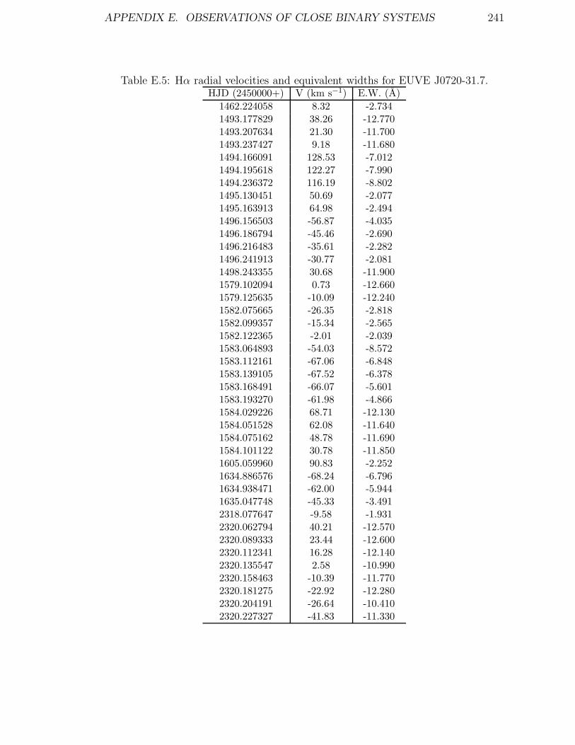
APPENDIX E. OBSERVATIONS OF CLOSE BINARY SYSTEMS 241
Table E.5: Hα radial velocities and equivalent widths for EUVE J0720-31.7.HJD (2450000+) V (km s−1) E.W. (A)
1462.224058 8.32 -2.7341493.177829 38.26 -12.7701493.207634 21.30 -11.7001493.237427 9.18 -11.6801494.166091 128.53 -7.0121494.195618 122.27 -7.9901494.236372 116.19 -8.8021495.130451 50.69 -2.0771495.163913 64.98 -2.4941496.156503 -56.87 -4.0351496.186794 -45.46 -2.6901496.216483 -35.61 -2.2821496.241913 -30.77 -2.0811498.243355 30.68 -11.9001579.102094 0.73 -12.6601579.125635 -10.09 -12.2401582.075665 -26.35 -2.8181582.099357 -15.34 -2.5651582.122365 -2.01 -2.0391583.064893 -54.03 -8.5721583.112161 -67.06 -6.8481583.139105 -67.52 -6.3781583.168491 -66.07 -5.6011583.193270 -61.98 -4.8661584.029226 68.71 -12.1301584.051528 62.08 -11.6401584.075162 48.78 -11.6901584.101122 30.78 -11.8501605.059960 90.83 -2.2521634.886576 -68.24 -6.7961634.938471 -62.00 -5.9441635.047748 -45.33 -3.4912318.077647 -9.58 -1.9312320.062794 40.21 -12.5702320.089333 23.44 -12.6002320.112341 16.28 -12.1402320.135547 2.58 -10.9902320.158463 -10.39 -11.7702320.181275 -22.92 -12.2802320.204191 -26.64 -10.4102320.227327 -41.83 -11.330

APPENDIX E. OBSERVATIONS OF CLOSE BINARY SYSTEMS 242
Table E.6: Hα radial velocities and equivalent widths for BPM 6502HJD (2450000+) V (km s−1) E.W. (A) HJD (2450000+) V (km s−1) E.W. (A)
1612.96021 28.2 -1.43 1641.01550 -65.5 -1.981613.02405 -44.2 -2.41 2301.078935 -41.37 -2.141613.04688 -55.6 -2.34 2301.102350 -50.06 -2.511613.07312 -59.6 -2.37 2301.125650 -50.54 -2.471613.09692 -47.8 -2.08 2301.148556 -55.12 -2.261613.11939 -33.7 -1.71 2301.171473 -27.74 -1.421614.10352 -58.5 -2.43 2302.014473 45.46 -1.821614.12622 -33.4 -1.83 2302.037691 14.85 -1.521614.14844 -9.2 -1.34 2302.061060 -16.23 -1.841614.17041 17.3 -1.03 2302.084163 -40.46 -1.951614.19226 51.0 -1.10 2302.107636 -57.37 -2.591614.21497 70.6 -1.21 2302.130959 -58.76 ...1614.23779 82.5 -1.47 2306.949260 47.26 ...1614.26001 76.4 -1.51 2316.938247 -55.37 -2.401614.28235 61.5 -1.29 2316.961338 -54.47 -2.641614.29919 43.3 -1.57 2316.984128 -39.86 -1.311634.91443 -43.6 -2.31 2317.007220 -25.72 -1.341634.97498 -60.8 -2.15 2317.041631 25.88 -1.061634.99854 -50.4 -1.77 2317.064711 57.83 -0.961635.02210 -18.2 -1.15 2317.088010 73.34 -1.091638.20190 55.1 -1.52 2317.110974 88.86 -1.561640.01917 -59.3 -2.22 2317.134366 77.87 -1.371640.04199 -48.4 -1.81 2317.157400 60.49 -1.511640.88513 61.5 -1.56 2317.180410 40.83 -1.791640.96741 -38.9 -2.04 2317.203987 -8.52 -2.651640.99036 -55.7 -2.04 2317.227078 -30.93 -1.53

APPENDIX E. OBSERVATIONS OF CLOSE BINARY SYSTEMS 243
Table E.7: Photometric measurements in R for BPM 71214HJD ∆R HJD ∆R HJD ∆R HJD ∆R HJD ∆R
(2452330+) mag (2452330+) mag (2452330+) mag (2452330+) mag (2452330+) mag
5.10327 -0.072 5.15967 -0.016 5.20312 -0.049 7.11401 -0.059 7.15869 -0.0255.10547 -0.061 5.16064 -0.006 5.20386 -0.053 7.11475 -0.059 7.15942 -0.0185.10644 -0.064 5.16138 -0.015 5.20459 -0.060 7.11548 -0.055 7.16016 -0.0225.10718 -0.068 5.16211 -0.009 5.20532 -0.054 7.11670 -0.063 7.16089 -0.0025.10815 -0.066 5.16284 -0.012 5.20654 -0.028 7.11743 -0.058 7.16162 -0.0235.10864 -0.075 5.16357 -0.026 5.20728 -0.047 7.11816 -0.070 7.16260 -0.0215.10962 -0.073 5.16431 -0.001 5.20801 -0.052 7.11890 -0.054 7.16333 -0.0105.11035 -0.074 5.16528 -0.014 5.20874 -0.049 7.11963 -0.055 7.16406 -0.0075.11108 -0.060 5.16602 -0.011 5.20947 -0.046 7.12061 -0.060 7.16480 -0.0195.11182 -0.056 5.16699 -0.011 5.21045 -0.039 7.12109 -0.070 7.16553 -0.0015.11255 -0.074 5.16772 -0.024 5.21118 -0.037 7.12207 -0.057 7.16650 -0.0255.11353 -0.069 5.16846 -0.026 5.21191 -0.026 7.12280 -0.074 7.16724 -0.0175.11426 -0.061 5.16919 -0.014 5.21265 -0.027 7.12354 -0.086 7.16821 -0.0155.11499 -0.058 5.17017 -0.023 5.21338 -0.030 7.12427 -0.062 7.16894 -0.0115.11572 -0.080 5.17090 -0.022 5.21436 -0.027 7.12500 -0.066 7.16968 -0.0305.11670 -0.073 5.17163 -0.029 5.21509 -0.035 7.12622 -0.079 7.17041 0.0045.11743 -0.070 5.17236 -0.030 5.21606 -0.009 7.12695 -0.069 7.17114 -0.0175.11816 -0.053 5.17310 -0.030 5.21680 -0.010 7.12769 -0.054 7.17212 -0.0165.11914 -0.060 5.17407 -0.020 5.21753 -0.024 7.12866 -0.055 7.17285 -0.0135.11987 -0.069 5.17481 -0.028 5.21826 -0.014 7.12939 -0.072 7.17358 -0.0105.12061 -0.069 5.17554 -0.033 5.21899 -0.017 7.13013 -0.080 7.17432 -0.0075.12134 -0.059 5.17651 -0.005 5.21997 -0.013 7.13086 -0.085 7.17505 -0.0115.12207 -0.051 5.17725 -0.027 5.22070 -0.014 7.13159 -0.072 7.17603 -0.0165.12305 -0.057 5.17798 -0.030 5.22144 0.002 7.13232 -0.107 7.17700 -0.0135.12378 -0.055 5.17871 -0.037 5.22217 -0.005 7.13306 -0.081 7.17773 -0.0165.12451 -0.063 5.17969 -0.043 5.22290 0.006 7.13403 -0.078 7.17847 -0.0155.12524 -0.058 5.18042 -0.041 5.22388 -0.012 7.13477 -0.061 7.17920 -0.0145.12622 -0.064 5.18115 -0.042 5.22461 0.003 7.13550 -0.056 7.18018 -0.0055.12695 -0.067 5.18188 -0.068 5.22534 0.008 7.13647 -0.068 7.18066 -0.0155.12769 -0.072 5.18262 -0.030 5.22632 0.015 7.13721 -0.073 7.18164 -0.0115.12866 -0.061 5.18359 -0.041 5.22705 0.010 7.13818 -0.089 7.18237 -0.0025.13037 -0.058 5.18433 -0.037 5.22778 0.003 7.13892 -0.079 7.18311 -0.0085.13110 -0.051 5.18506 -0.039 5.22852 0.010 7.13965 -0.057 7.18384 -0.0095.13184 -0.059 5.18579 -0.051 5.22949 0.014 7.14038 -0.074 7.18457 -0.0275.13257 -0.058 5.18677 -0.041 5.23022 0.031 7.14111 -0.058 7.18555 -0.0155.13355 -0.060 5.18774 -0.037 5.23096 0.000 7.14185 -0.054 7.18652 -0.0205.13428 -0.053 5.18848 -0.049 5.23193 0.014 7.14258 -0.055 7.18726 -0.0315.13501 -0.048 5.18921 -0.058 5.23267 0.018 7.14356 -0.059 7.18799 -0.0185.13574 -0.031 5.18994 -0.044 5.23340 0.022 7.14429 -0.058 7.18872 -0.0345.13672 -0.050 5.19067 -0.042 7.10132 -0.013 7.14502 -0.056 7.18970 -0.0335.13769 -0.044 5.19165 -0.058 7.10205 -0.027 7.14575 -0.071 7.19043 -0.0275.13818 -0.054 5.19238 -0.054 7.10303 -0.023 7.14673 -0.015 7.19116 -0.0245.13916 -0.047 5.19312 -0.059 7.10376 -0.031 7.14770 -0.031 7.19189 -0.0305.13989 -0.053 5.19385 -0.051 7.10449 -0.017 7.14844 -0.051 7.19263 -0.0295.14062 -0.036 5.19458 -0.053 7.10522 -0.030 7.14917 -0.054 7.19336 -0.0335.14136 -0.041 5.19531 -0.057 7.10620 -0.041 7.15063 -0.039 7.19409 -0.0285.14209 -0.040 5.19629 -0.058 7.10718 -0.044 7.15137 -0.033 7.19507 -0.0325.14307 -0.027 5.19727 -0.053 7.10791 -0.039 7.15210 -0.035 7.19580 -0.0535.14380 -0.016 5.19800 -0.061 7.10864 -0.035 7.15308 -0.024 7.19678 -0.0445.14453 -0.022 5.19873 -0.047 7.10938 -0.049 7.15381 -0.027 7.19751 -0.0405.14526 -0.019 5.19946 -0.054 7.11011 -0.046 7.15454 -0.030 7.19922 -0.0495.14624 -0.034 5.19995 -0.039 7.11108 -0.043 7.15527 -0.030 7.19995 -0.0535.14697 -0.029 5.20093 -0.040 7.11157 -0.047 7.15625 -0.024 7.20044 -0.0445.14868 -0.009 5.20166 -0.046 7.11255 -0.059 7.15698 -0.033 7.20117 -0.0535.15894 -0.012 5.20239 -0.061 7.11328 -0.047 7.15771 -0.017 7.20190 -0.048
Continues on next page
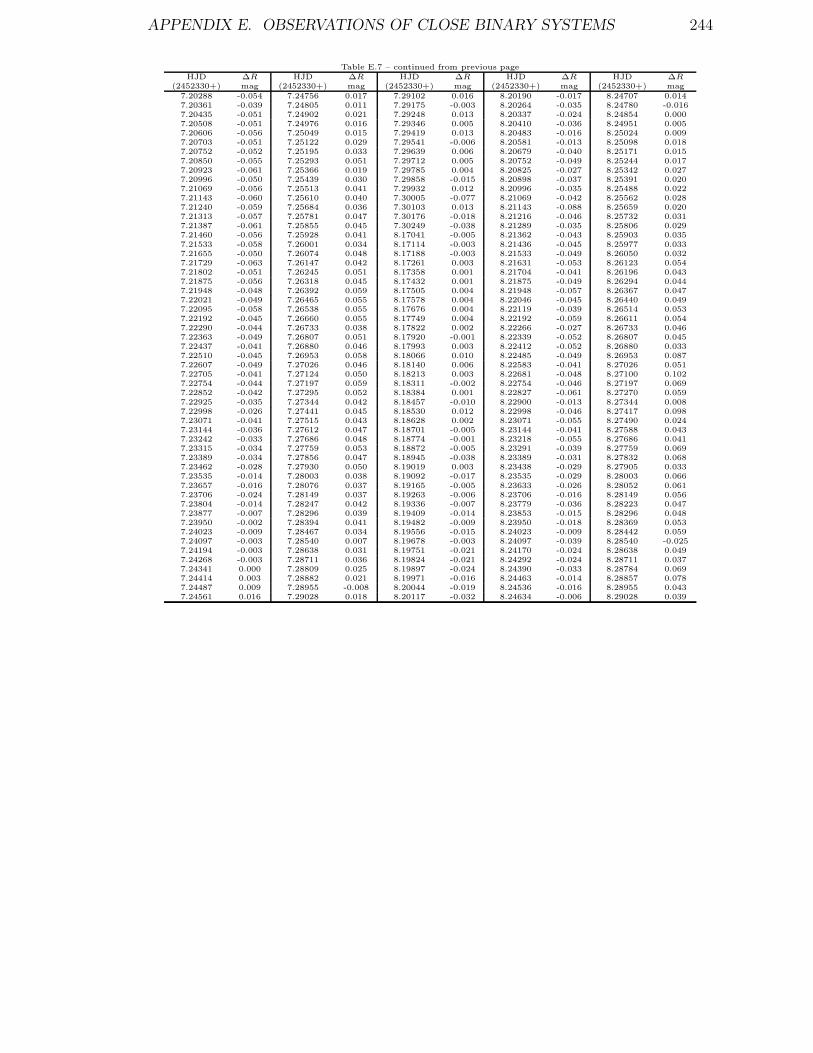
APPENDIX E. OBSERVATIONS OF CLOSE BINARY SYSTEMS 244
Table E.7 – continued from previous pageHJD ∆R HJD ∆R HJD ∆R HJD ∆R HJD ∆R
(2452330+) mag (2452330+) mag (2452330+) mag (2452330+) mag (2452330+) mag7.20288 -0.054 7.24756 0.017 7.29102 0.016 8.20190 -0.017 8.24707 0.0147.20361 -0.039 7.24805 0.011 7.29175 -0.003 8.20264 -0.035 8.24780 -0.0167.20435 -0.051 7.24902 0.021 7.29248 0.013 8.20337 -0.024 8.24854 0.0007.20508 -0.051 7.24976 0.016 7.29346 0.005 8.20410 -0.036 8.24951 0.0057.20606 -0.056 7.25049 0.015 7.29419 0.013 8.20483 -0.016 8.25024 0.0097.20703 -0.051 7.25122 0.029 7.29541 -0.006 8.20581 -0.013 8.25098 0.0187.20752 -0.052 7.25195 0.033 7.29639 0.006 8.20679 -0.040 8.25171 0.0157.20850 -0.055 7.25293 0.051 7.29712 0.005 8.20752 -0.049 8.25244 0.0177.20923 -0.061 7.25366 0.019 7.29785 0.004 8.20825 -0.027 8.25342 0.0277.20996 -0.050 7.25439 0.030 7.29858 -0.015 8.20898 -0.037 8.25391 0.0207.21069 -0.056 7.25513 0.041 7.29932 0.012 8.20996 -0.035 8.25488 0.0227.21143 -0.060 7.25610 0.040 7.30005 -0.077 8.21069 -0.042 8.25562 0.0287.21240 -0.059 7.25684 0.036 7.30103 0.013 8.21143 -0.088 8.25659 0.0207.21313 -0.057 7.25781 0.047 7.30176 -0.018 8.21216 -0.046 8.25732 0.0317.21387 -0.061 7.25855 0.045 7.30249 -0.038 8.21289 -0.035 8.25806 0.0297.21460 -0.056 7.25928 0.041 8.17041 -0.005 8.21362 -0.043 8.25903 0.0357.21533 -0.058 7.26001 0.034 8.17114 -0.003 8.21436 -0.045 8.25977 0.0337.21655 -0.050 7.26074 0.048 8.17188 -0.003 8.21533 -0.049 8.26050 0.0327.21729 -0.063 7.26147 0.042 8.17261 0.003 8.21631 -0.053 8.26123 0.0547.21802 -0.051 7.26245 0.051 8.17358 0.001 8.21704 -0.041 8.26196 0.0437.21875 -0.056 7.26318 0.045 8.17432 0.001 8.21875 -0.049 8.26294 0.0447.21948 -0.048 7.26392 0.059 8.17505 0.004 8.21948 -0.057 8.26367 0.0477.22021 -0.049 7.26465 0.055 8.17578 0.004 8.22046 -0.045 8.26440 0.0497.22095 -0.058 7.26538 0.055 8.17676 0.004 8.22119 -0.039 8.26514 0.0537.22192 -0.045 7.26660 0.055 8.17749 0.004 8.22192 -0.059 8.26611 0.0547.22290 -0.044 7.26733 0.038 8.17822 0.002 8.22266 -0.027 8.26733 0.0467.22363 -0.049 7.26807 0.051 8.17920 -0.001 8.22339 -0.052 8.26807 0.0457.22437 -0.041 7.26880 0.046 8.17993 0.003 8.22412 -0.052 8.26880 0.0337.22510 -0.045 7.26953 0.058 8.18066 0.010 8.22485 -0.049 8.26953 0.0877.22607 -0.049 7.27026 0.046 8.18140 0.006 8.22583 -0.041 8.27026 0.0517.22705 -0.041 7.27124 0.050 8.18213 0.003 8.22681 -0.048 8.27100 0.1027.22754 -0.044 7.27197 0.059 8.18311 -0.002 8.22754 -0.046 8.27197 0.0697.22852 -0.042 7.27295 0.052 8.18384 0.001 8.22827 -0.061 8.27270 0.0597.22925 -0.035 7.27344 0.042 8.18457 -0.010 8.22900 -0.013 8.27344 0.0087.22998 -0.026 7.27441 0.045 8.18530 0.012 8.22998 -0.046 8.27417 0.0987.23071 -0.041 7.27515 0.043 8.18628 0.002 8.23071 -0.055 8.27490 0.0247.23144 -0.036 7.27612 0.047 8.18701 -0.005 8.23144 -0.041 8.27588 0.0437.23242 -0.033 7.27686 0.048 8.18774 -0.001 8.23218 -0.055 8.27686 0.0417.23315 -0.034 7.27759 0.053 8.18872 -0.005 8.23291 -0.039 8.27759 0.0697.23389 -0.034 7.27856 0.047 8.18945 -0.038 8.23389 -0.031 8.27832 0.0687.23462 -0.028 7.27930 0.050 8.19019 0.003 8.23438 -0.029 8.27905 0.0337.23535 -0.014 7.28003 0.038 8.19092 -0.017 8.23535 -0.029 8.28003 0.0667.23657 -0.016 7.28076 0.037 8.19165 -0.005 8.23633 -0.026 8.28052 0.0617.23706 -0.024 7.28149 0.037 8.19263 -0.006 8.23706 -0.016 8.28149 0.0567.23804 -0.014 7.28247 0.042 8.19336 -0.007 8.23779 -0.036 8.28223 0.0477.23877 -0.007 7.28296 0.039 8.19409 -0.014 8.23853 -0.015 8.28296 0.0487.23950 -0.002 7.28394 0.041 8.19482 -0.009 8.23950 -0.018 8.28369 0.0537.24023 -0.009 7.28467 0.034 8.19556 -0.015 8.24023 -0.009 8.28442 0.0597.24097 -0.003 7.28540 0.007 8.19678 -0.003 8.24097 -0.039 8.28540 -0.0257.24194 -0.003 7.28638 0.031 8.19751 -0.021 8.24170 -0.024 8.28638 0.0497.24268 -0.003 7.28711 0.036 8.19824 -0.021 8.24292 -0.024 8.28711 0.0377.24341 0.000 7.28809 0.025 8.19897 -0.024 8.24390 -0.033 8.28784 0.0697.24414 0.003 7.28882 0.021 8.19971 -0.016 8.24463 -0.014 8.28857 0.0787.24487 0.009 7.28955 -0.008 8.20044 -0.019 8.24536 -0.016 8.28955 0.0437.24561 0.016 7.29028 0.018 8.20117 -0.032 8.24634 -0.006 8.29028 0.039

APPENDIX E. OBSERVATIONS OF CLOSE BINARY SYSTEMS 245
Table E.8: Photometric measurements in I for BPM 71214HJD ∆I HJD ∆I HJD ∆I HJD ∆I HJD ∆I
(2452330+) mag (2452330+) mag (2452330+) mag (2452330+) mag (2452330+) mag
9.09832 0.024 9.14594 -0.034 9.18483 0.014 9.22448 -0.027 9.26558 0.0349.09892 0.035 9.14654 -0.029 9.18544 0.018 9.22510 -0.035 9.26618 0.0219.09953 0.046 9.14715 -0.036 9.18604 0.021 9.22569 -0.037 9.26677 0.0229.10012 0.034 9.14775 -0.033 9.18665 0.022 9.22630 -0.034 9.26738 0.0299.10074 0.034 9.14836 -0.036 9.18726 0.015 9.22692 -0.035 9.26799 0.0249.10135 0.024 9.14895 -0.028 9.18786 0.017 9.22752 -0.026 9.26860 0.0169.10254 0.029 9.14956 -0.025 9.18846 0.017 9.22811 -0.025 9.26948 0.0289.10921 0.015 9.15017 -0.028 9.18907 0.028 9.22872 -0.039 9.27008 0.0439.10982 0.019 9.15078 -0.031 9.18968 0.018 9.22933 -0.032 9.27069 0.0369.11043 0.010 9.15137 -0.026 9.19028 0.015 9.23116 -0.033 9.27129 0.0469.11103 0.005 9.15198 -0.039 9.19088 0.022 9.23177 -0.025 9.27190 0.0289.11164 0.008 9.15258 -0.026 9.19150 0.018 9.23237 -0.021 9.27250 0.0369.11224 0.011 9.15320 -0.032 9.19210 0.022 9.23298 -0.039 9.27309 0.0439.11285 0.004 9.15380 -0.016 9.19351 0.021 9.23358 -0.033 9.27369 0.0329.11346 0.001 9.15440 -0.026 9.19412 0.012 9.23420 -0.045 9.27673 0.0449.11406 0.012 9.15501 -0.016 9.19474 0.009 9.23479 -0.034 9.27734 0.0549.11466 -0.006 9.15609 -0.019 9.19534 0.007 9.23539 -0.031 9.27793 0.0479.11528 -0.001 9.15670 -0.023 9.19594 0.005 9.23600 -0.032 9.27853 0.0499.11588 -0.004 9.15730 -0.021 9.19655 0.008 9.23662 -0.036 9.27913 0.0449.11923 -0.003 9.15789 -0.022 9.19716 0.012 9.23721 -0.032 9.27975 0.0469.11984 -0.008 9.15850 -0.012 9.19775 0.015 9.23782 -0.032 9.28036 0.0559.12044 -0.002 9.15911 -0.014 9.19836 0.009 9.23843 -0.027 9.28095 0.0519.12105 -0.016 9.15971 -0.013 9.19897 0.008 9.23903 -0.032 9.28155 0.0449.12165 -0.014 9.16031 -0.019 9.19958 0.002 9.23965 -0.034 9.28215 0.0449.12226 -0.015 9.16094 -0.017 9.20018 0.004 9.24024 -0.030 9.28275 0.0439.12286 -0.043 9.16154 -0.011 9.20078 0.005 9.24086 -0.032 9.28338 0.0559.12347 -0.037 9.16215 -0.016 9.20139 -0.002 9.24145 -0.032 9.28398 0.0519.12407 -0.039 9.16276 -0.001 9.20199 0.003 9.24208 -0.026 9.28458 0.0549.12466 -0.019 9.16337 -0.013 9.20259 -0.004 9.24267 -0.019 9.28517 0.0479.12529 -0.020 9.16397 -0.008 9.20320 0.008 9.24328 -0.024 9.28577 0.0549.12589 -0.022 9.16456 -0.003 9.20380 0.007 9.24390 -0.026 9.28638 0.0389.12649 -0.024 9.16518 -0.010 9.20441 0.003 9.24450 -0.020 9.28700 0.0609.12711 -0.034 9.16579 -0.006 9.20502 -0.002 9.24511 -0.022 9.28796 0.0679.12771 -0.028 9.16639 0.003 9.20561 0.002 9.24570 -0.010 9.28855 0.0589.12831 -0.037 9.16698 -0.012 9.20622 0.000 9.24633 -0.029 9.28915 0.0509.12892 -0.018 9.16759 -0.010 9.20742 -0.007 9.24692 -0.029 9.28977 0.0699.12952 -0.024 9.16820 0.001 9.20803 -0.004 9.24754 -0.020 9.29037 0.0569.13013 -0.026 9.16880 -0.005 9.20864 -0.011 9.24814 -0.015 9.29097 0.0599.13074 -0.026 9.16940 0.001 9.20923 -0.007 9.24873 -0.025 9.29158 0.0569.13134 -0.035 9.17001 0.003 9.20983 -0.007 9.25107 -0.020 9.29220 0.0449.13194 -0.023 9.17060 -0.011 9.21044 -0.015 9.25166 -0.010 9.29280 0.0569.13255 -0.022 9.17122 -0.001 9.21106 -0.010 9.25226 -0.007 9.29340 0.0559.13316 -0.024 9.17183 0.004 9.21179 -0.015 9.25288 -0.011 9.29401 0.0539.13377 -0.023 9.17243 0.014 9.21239 -0.014 9.25348 -0.014 9.29462 0.0439.13436 -0.029 9.17303 0.012 9.21298 -0.015 9.25409 -0.004 9.29522 0.0449.13498 -0.038 9.17364 0.005 9.21359 -0.030 9.25469 -0.006 9.29581 0.0459.13559 -0.038 9.17456 0.011 9.21419 -0.014 9.25530 -0.003 9.29641 0.0479.13618 -0.041 9.17518 0.015 9.21481 -0.020 9.25589 0.002 9.29701 0.0449.13679 -0.027 9.17577 0.011 9.21540 -0.024 9.25650 -0.005 9.29764 0.0799.13747 -0.038 9.17638 0.004 9.21601 -0.026 9.25710 0.007 9.29824 0.0449.13808 -0.049 9.17699 0.007 9.21663 -0.030 9.25772 0.009 9.29884 0.0469.13868 -0.041 9.17760 0.010 9.21722 -0.024 9.25832 0.002 9.29943 0.0439.13927 -0.025 9.17819 0.005 9.21782 -0.024 9.25892 0.006 9.30003 0.0539.13987 -0.033 9.17880 0.002 9.21843 -0.018 9.25953 0.010 9.30066 0.0489.14050 -0.027 9.17940 0.022 9.21903 -0.016 9.26014 0.022 9.30126 0.0349.14110 -0.030 9.18001 0.017 9.21965 -0.014 9.26074 0.016 9.30185 0.0259.14170 -0.033 9.18062 0.010 9.22025 -0.023 9.26133 0.008 9.30245 0.0479.14231 -0.029 9.18121 0.016 9.22086 -0.026 9.26193 0.017 9.30308 0.0199.14291 -0.033 9.18182 0.015 9.22146 -0.036 9.26254 0.010 9.30368 0.0329.14352 -0.033 9.18242 0.012 9.22205 -0.028 9.26316 0.017 9.30427 0.0499.14413 -0.036 9.18302 0.011 9.22266 -0.020 9.26376 0.021 9.30488 0.0379.14473 -0.017 9.18364 0.011 9.22327 -0.029 9.26435 0.023 9.30550 0.0119.14532 -0.034 9.18424 0.020 9.22388 -0.031 9.26497 0.028 0.00000 0.000

APPENDIX E. OBSERVATIONS OF CLOSE BINARY SYSTEMS 246
Table E.9: Photometric measurements in B for EC 13471−1258HJD ∆B HJD ∆B HJD ∆B HJD ∆B HJD ∆B
(2452380+) mag (2452380+) mag (2452380+) mag (2452380+) mag (2452380+) mag
3.10262 -0.022 3.14886 -0.035 3.18931 0.018 3.23334 -0.009 4.08531 0.0013.10332 -0.025 3.14958 -0.040 3.19004 0.010 3.23406 -0.002 4.08601 0.0083.10404 -0.014 3.15029 -0.015 3.19074 0.033 3.23479 -0.024 4.08674 0.0143.10550 0.001 3.15102 -0.020 3.19147 -0.002 3.23623 -0.026 4.08747 0.0133.10620 0.008 3.15175 -0.021 3.19508 1.830 3.23696 -0.028 4.08818 0.0313.10693 0.008 3.15246 -0.018 3.19579 1.878 3.23768 -0.017 4.08891 0.0153.10765 -0.003 3.15318 -0.029 3.19652 1.944 3.23838 -0.008 4.08963 0.0283.10910 0.010 3.15390 -0.026 3.19725 1.868 3.23911 -0.025 4.09035 0.0183.10980 -0.011 3.15462 -0.045 3.19795 1.854 3.23984 -0.015 4.09107 0.0213.11055 0.009 3.15533 -0.029 3.19941 1.861 3.24055 -0.015 4.09179 0.0193.11198 0.001 3.15605 -0.029 3.20012 1.885 3.24128 -0.005 4.09249 0.0163.11271 0.027 3.15678 -0.045 3.20085 1.859 3.24200 -0.057 4.09395 0.0353.11343 -0.047 3.15749 -0.034 3.20229 1.896 3.24271 -0.012 4.09467 0.0233.11414 0.015 3.15822 -0.043 3.20301 1.897 3.24344 -0.021 4.09538 0.0223.11487 0.016 3.15895 -0.053 3.20374 1.917 3.24417 -0.038 4.09610 0.0363.11559 0.004 3.15967 -0.046 3.20446 1.806 3.24487 -0.014 4.09682 0.0323.11631 -0.007 3.16038 -0.036 3.20516 0.061 3.24559 -0.030 4.09755 0.0233.11703 0.011 3.16183 -0.020 3.20589 0.037 3.24703 -0.009 4.09826 0.0343.11773 0.000 3.16255 -0.039 3.20662 0.030 3.24777 -0.044 4.09898 0.4223.11846 0.033 3.16325 -0.046 3.20733 0.081 3.24849 -0.003 4.10114 1.8803.11919 -0.054 3.16398 -0.034 3.20806 0.043 3.24919 -0.021 4.10188 1.8853.12136 -0.004 3.16471 -0.050 3.20879 0.019 3.24992 -0.039 4.10260 1.8783.12280 0.014 3.16543 0.007 3.20949 0.030 3.25065 0.003 4.10330 1.8873.12351 0.014 3.16616 -0.034 3.21022 0.025 3.25209 -0.033 4.10403 1.8823.12497 0.016 3.16688 -0.023 3.21095 0.022 3.25281 -0.032 4.10476 1.8663.12568 0.023 3.16759 -0.041 3.21167 0.033 3.25353 0.051 4.10547 1.9033.12640 0.006 3.16832 -0.031 3.21239 0.037 3.25425 -0.010 4.10619 1.8933.12711 0.016 3.16903 -0.019 3.21310 0.007 3.25498 -0.027 4.10693 1.8743.12784 0.015 3.16976 -0.027 3.21383 -0.020 3.25570 -0.034 4.10763 1.8633.12855 0.008 3.17049 -0.012 3.21455 0.043 3.25643 -0.002 4.10836 1.9033.12927 0.032 3.17121 -0.024 3.21527 0.045 3.25714 -0.021 4.10909 1.6253.13000 0.014 3.17192 -0.009 3.21600 0.018 3.25785 -0.029 4.10980 0.0313.13071 0.010 3.17264 -0.001 3.21671 0.018 3.25858 -0.013 4.11051 0.0423.13145 0.002 3.17335 -0.004 3.21743 0.007 3.25931 -0.007 4.11197 0.0463.13215 0.020 3.17409 -0.015 3.21814 0.003 3.26003 -0.015 4.11269 -0.0173.13287 0.003 3.17480 -0.001 3.21887 -0.013 3.26074 -0.021 4.11342 0.0073.13361 0.018 3.17552 0.009 3.21960 0.010 3.26146 0.011 4.11413 0.0133.13433 0.009 3.17625 -0.013 3.22030 -0.001 3.26218 0.013 4.11484 -0.0013.13504 0.021 3.17697 0.000 3.22103 0.012 3.26291 0.017 4.11556 0.0233.13649 0.014 3.17768 0.002 3.22176 -0.026 3.26361 0.017 4.11629 0.0103.13721 0.003 3.17840 0.005 3.22248 0.030 3.26434 0.040 4.11701 -0.0113.13793 0.002 3.17913 0.005 3.22318 0.002 3.26507 -0.006 4.11774 0.0173.13866 -0.011 3.17984 0.064 3.22391 0.017 3.26578 0.008 4.11845 0.0053.13938 -0.017 3.18057 0.000 3.22464 0.022 3.26651 0.031 4.11917 -0.0063.14009 -0.008 3.18130 0.010 3.22535 -0.001 3.26724 -0.004 4.11990 0.0163.14082 -0.007 3.18200 0.019 3.22608 0.010 3.26794 0.056 4.12062 0.0133.14154 0.002 3.18273 0.008 3.22681 -0.016 3.26867 0.002 4.12134 0.0193.14226 -0.026 3.18346 0.003 3.22752 -0.011 3.26940 -0.005 4.12207 0.0203.14299 -0.013 3.18417 0.004 3.22824 -0.011 3.27012 0.049 4.12278 0.0003.14369 -0.027 3.18490 0.016 3.22895 -0.004 3.27084 0.086 4.12350 0.0143.14442 -0.039 3.18563 0.006 3.22968 -0.011 3.27299 0.048 4.12423 -0.0033.14514 -0.029 3.18633 0.023 3.23041 -0.011 3.27515 0.039 4.12495 0.0103.14597 -0.032 3.18706 0.021 3.23111 0.001 4.08301 -0.003 4.12568 0.0183.14742 -0.014 3.18779 0.020 3.23184 0.018 4.08386 0.010 4.12639 -0.0043.14813 -0.021 3.18850 0.013 3.23263 0.009 4.08458 0.007

APPENDIX E. OBSERVATIONS OF CLOSE BINARY SYSTEMS 247
Table E.10: Photometric measurements in R for EC 13471−1258HJD ∆R HJD ∆R HJD ∆R HJD ∆R HJD ∆R
(2452380+) mag (2452380+) mag (2452380+) mag (2452380+) mag (2452380+) mag
4.14255 -0.072 4.18235 0.088 4.22207 -0.100 4.26253 0.053 6.07986 0.0514.14345 -0.090 4.18308 0.093 4.22279 -0.103 4.26327 0.066 6.08059 0.0534.14417 -0.086 4.18381 0.081 4.22351 -0.120 4.26398 0.054 6.08130 -0.0314.14489 -0.073 4.18452 0.093 4.22424 -0.104 4.26469 0.067 6.08201 0.0404.14560 -0.084 4.18525 0.087 4.22495 -0.099 4.26543 0.084 6.08274 0.0314.14632 -0.066 4.18598 0.080 4.22569 -0.089 4.26615 0.044 6.08346 0.0344.14705 -0.075 4.18674 0.070 4.22641 -0.065 4.26686 0.055 6.08419 0.0304.14777 -0.075 4.18746 0.071 4.22711 -0.092 4.26760 0.050 6.08490 0.0184.14848 -0.072 4.18819 0.054 4.22783 -0.059 4.26832 0.023 6.08562 0.0084.14921 -0.071 4.18889 0.065 4.22856 -0.070 4.26902 0.029 6.08634 0.0254.14994 -0.073 4.18962 0.057 4.22928 -0.097 4.26975 0.004 6.08705 0.0254.15064 -0.072 4.19034 0.056 4.23009 -0.068 4.27048 0.059 6.08777 0.0064.15137 -0.051 4.19106 0.045 4.23080 -0.083 4.27119 0.034 6.08849 -0.0054.15210 -0.049 4.19179 0.040 4.23152 -0.050 4.27190 0.062 6.08920 -0.0034.15281 -0.056 4.19249 0.032 4.23297 -0.060 4.27264 0.008 6.08993 -0.0344.15355 -0.044 4.19321 0.031 4.23370 -0.045 4.27343 -0.012 6.09064 -0.0244.15427 -0.047 4.19394 0.025 4.23440 -0.050 4.27489 -0.008 6.09135 -0.0344.15498 -0.039 4.19466 0.019 4.23513 -0.034 4.27560 -0.007 6.09207 -0.0474.15571 -0.036 4.19538 0.009 4.23586 -0.040 4.27631 0.005 6.09279 -0.0224.15643 -0.027 4.19610 -0.001 4.23657 -0.015 4.27705 0.017 6.09351 -0.0524.15713 -0.024 4.19683 -0.018 4.23729 -0.016 4.27777 0.009 6.09423 -0.0464.15786 -0.014 4.19754 -0.026 4.23801 -0.007 4.27848 -0.036 6.09494 -0.0454.15857 -0.017 4.19827 -0.024 4.23873 0.029 4.27920 -0.009 6.09567 -0.0584.15931 -0.012 4.19899 -0.026 4.23946 0.017 4.27994 0.004 6.09637 -0.0504.16003 -0.001 4.19973 -0.040 4.24017 0.011 4.28136 -0.032 6.09710 -0.0604.16073 0.002 4.20043 -0.044 4.24090 0.006 4.28210 -0.102 6.09782 -0.0554.16146 -0.006 4.20115 -0.049 4.24161 0.016 4.28282 -0.009 6.09855 -0.0864.16219 0.022 4.20188 -0.053 4.24233 0.000 4.28352 -0.111 6.09927 -0.0804.16290 0.016 4.20260 -0.061 4.24306 0.007 4.28424 -0.014 6.09998 -0.0764.16363 0.020 4.20333 -0.074 4.24378 0.055 4.28569 -0.078 6.10069 -0.0754.16436 0.025 4.20404 -0.061 4.24450 0.042 4.28786 -0.045 6.10141 -0.0564.16507 0.020 4.20476 -0.072 4.24523 0.045 4.29003 -0.039 6.10214 -0.0784.16578 0.030 4.20548 -0.073 4.24595 0.045 4.29145 -0.088 6.10286 -0.0874.16651 0.044 4.20621 -0.081 4.24666 0.065 4.29219 -0.044 6.10356 -0.1064.16724 0.038 4.20692 -0.090 4.24739 0.060 4.29291 -0.163 6.10428 -0.0914.16795 0.054 4.20764 -0.090 4.24812 0.052 4.29362 -0.091 6.10500 -0.0904.16869 0.065 4.20837 -0.080 4.24883 0.066 4.29436 -0.084 6.10571 -0.0814.16940 0.072 4.20910 -0.095 4.24957 0.083 6.06677 0.406 6.10642 -0.0674.17011 0.063 4.20981 -0.100 4.25027 0.356 6.06748 0.389 6.10715 -0.0784.17085 0.081 4.21053 -0.105 4.25099 0.371 6.06819 0.409 6.10787 -0.0764.17157 0.083 4.21126 -0.105 4.25173 0.388 6.06892 0.393 6.10858 -0.0604.17227 0.071 4.21198 -0.108 4.25244 0.380 6.06964 0.090 6.10930 -0.0604.17300 0.102 4.21269 -0.116 4.25315 0.395 6.07036 0.091 6.11003 -0.0884.17373 0.087 4.21342 -0.108 4.25389 0.382 6.07107 0.094 6.11075 -0.0784.17444 0.090 4.21415 -0.111 4.25460 0.357 6.07179 0.085 6.11147 -0.0364.17517 0.085 4.21486 -0.123 4.25532 0.386 6.07268 0.076 6.11217 -0.0454.17589 0.096 4.21558 -0.106 4.25606 0.405 6.07341 0.077 6.11289 -0.0784.17660 0.097 4.21630 -0.111 4.25678 0.401 6.07413 0.072 6.11362 -0.0464.17732 0.099 4.21702 -0.109 4.25748 0.377 6.07483 0.069 6.11433 -0.0354.17805 0.104 4.21774 -0.114 4.25821 0.402 6.07556 0.074 6.11504 -0.0334.17876 0.097 4.21847 -0.110 4.25894 0.369 6.07628 0.067 6.11604 -0.0264.17948 0.097 4.21918 -0.112 4.25965 0.396 6.07699 0.066 6.11674 -0.0214.18019 0.100 4.21990 -0.105 4.26036 0.069 6.07772 0.051 6.11746 -0.0254.18092 0.107 4.22063 -0.111 4.26111 0.075 6.07843 0.065 6.11818 -0.0054.18165 0.096 4.22136 -0.100 4.26181 0.092 6.07914 0.056 6.11890 -0.013
Continues on next page

APPENDIX E. OBSERVATIONS OF CLOSE BINARY SYSTEMS 248
Table E.10 – continued from previous pageHJD ∆R HJD ∆R HJD ∆R HJD ∆R HJD ∆R
(2452380+) mag (2452380+) mag (2452380+) mag (2452380+) mag (2452380+) mag6.11961 -0.006 6.16073 -0.028 6.19015 -0.045 6.21702 0.415 6.24360 -0.0546.12033 0.006 6.16144 -0.041 6.19088 -0.052 6.21775 0.401 6.24430 -0.0446.12105 -0.006 6.16216 -0.042 6.19158 -0.052 6.21847 0.413 6.24503 -0.0596.12176 0.000 6.16288 -0.058 6.19231 -0.045 6.21919 0.414 6.24575 -0.0696.12248 -0.002 6.16360 -0.054 6.19302 -0.053 6.21990 0.251 6.26244 -0.0726.12320 0.039 6.16431 -0.057 6.19373 -0.036 6.22062 0.091 6.26316 -0.0786.12390 0.023 6.16503 -0.090 6.19445 -0.033 6.22133 0.079 6.26387 -0.0486.12463 0.012 6.16574 -0.125 6.19516 -0.017 6.22204 0.090 6.26459 -0.0836.12607 0.064 6.16717 -0.083 6.19589 -0.019 6.22275 0.091 6.26531 -0.0286.12678 0.051 6.16789 -0.109 6.19662 -0.017 6.22348 0.096 6.26601 0.0106.12751 0.054 6.16862 -0.139 6.19732 0.000 6.22421 0.100 6.26674 -0.0956.12821 0.076 6.16935 -0.119 6.19804 0.006 6.22492 0.079 6.26745 -0.0466.12894 0.068 6.17005 -0.121 6.19877 0.020 6.22563 0.068 6.26817 -0.0376.13252 0.136 6.17078 -0.061 6.19948 0.030 6.22635 0.087 6.26890 -0.0446.13394 0.104 6.17221 -0.105 6.20020 0.023 6.22706 0.077 6.26960 -0.0596.13466 0.095 6.17292 -0.117 6.20092 0.016 6.22779 0.062 6.27033 -0.0356.13539 0.100 6.17363 -0.119 6.20163 0.047 6.22849 0.062 6.27105 0.0276.14687 0.081 6.17435 -0.121 6.20340 0.041 6.22922 0.092 6.27174 0.0266.14758 0.079 6.17508 -0.121 6.20412 0.062 6.22994 0.054 6.27247 0.0086.14831 0.060 6.17580 -0.104 6.20485 0.061 6.23066 0.062 6.27319 0.0296.14902 0.073 6.17652 -0.134 6.20556 0.060 6.23139 0.069 6.27390 0.0396.14974 0.058 6.17723 -0.142 6.20627 0.061 6.23282 0.026 6.27463 0.0136.15046 0.061 6.17794 -0.103 6.20699 0.078 6.23353 0.036 6.27533 0.0776.15117 0.040 6.17867 -0.145 6.20772 0.075 6.23424 0.026 6.27606 0.0676.15189 0.038 6.17938 -0.104 6.20842 0.066 6.23496 0.031 6.27678 0.0326.15260 0.035 6.18010 -0.049 6.20915 0.075 6.23568 0.018 6.27748 0.0466.15332 0.012 6.18298 -0.076 6.20987 0.357 6.23640 0.020 6.27820 0.0126.15404 0.037 6.18369 -0.111 6.21059 0.413 6.23713 0.023 6.27893 0.0356.15475 0.017 6.18441 -0.098 6.21129 0.402 6.23784 0.007 6.27964 0.0646.15548 0.012 6.18511 -0.107 6.21201 0.409 6.23855 -0.007 6.28036 0.0776.15620 -0.006 6.18584 -0.084 6.21272 0.396 6.23927 -0.008 6.28108 0.0826.15692 0.011 6.18655 -0.076 6.21345 0.424 6.24000 -0.003 6.28180 0.0476.15764 -0.026 6.18728 -0.094 6.21417 0.414 6.24071 -0.013 6.28252 0.1196.15835 -0.017 6.18799 -0.055 6.21488 0.416 6.24143 -0.036 6.28324 0.0606.15929 -0.007 6.18871 -0.070 6.21561 0.412 6.24214 -0.0176.16000 -0.041 6.18944 -0.064 6.21632 0.421 6.24287 -0.028

APPENDIX E. OBSERVATIONS OF CLOSE BINARY SYSTEMS 249
Table E.11: Photometric measurements in R for BPM 6502HJD ∆R HJD ∆R HJD ∆R HJD ∆R HJD ∆R
(2452000+) mag (2452000+) mag (2452000+) mag (2452000+) mag (2452000+) mag192.26969 -0.017 263.13577 0.019 263.27751 0.001 265.24165 -0.006 266.29484 -0.015192.27642 -0.010 263.13978 0.018 263.28161 -0.012 265.25048 -0.006 266.30363 -0.019192.28314 -0.017 263.14379 0.019 263.28574 -0.008 265.25934 -0.008 266.31248 -0.012192.28987 -0.013 263.14780 0.014 263.28983 -0.004 265.26812 -0.006 266.32377 -0.015192.29660 -0.011 263.15181 0.016 263.29388 -0.013 265.27695 -0.009 266.33259 -0.017192.30334 -0.009 263.15583 0.010 263.30563 -0.009 265.28575 -0.009 267.06969 -0.001192.31948 -0.009 263.15986 0.014 263.30969 -0.004 265.29458 -0.017 267.07445 -0.005192.32761 -0.005 263.16389 0.018 263.31375 -0.014 265.30340 -0.014 267.08320 -0.007192.33577 -0.012 263.16802 0.008 263.31790 -0.009 265.31229 -0.015 267.09196 0.002192.34389 -0.012 263.17206 0.011 263.32197 -0.012 265.32117 -0.009 267.10083 -0.007192.35201 -0.009 263.17609 0.010 263.32604 -0.008 265.33012 -0.014 267.10964 0.003193.25235 -0.020 263.18011 0.016 263.33011 -0.012 266.08056 0.013 267.11849 -0.005193.26103 -0.007 263.18414 0.013 263.33419 -0.009 266.08934 0.005 267.12727 0.003193.26916 -0.010 263.18817 0.012 263.33824 -0.010 266.09813 0.009 267.13620 -0.002193.27731 -0.011 263.19221 0.005 263.34231 -0.011 266.10693 0.023 267.14506 -0.005193.28549 -0.009 263.19995 0.007 263.34635 -0.007 266.11573 0.015 267.15384 0.000193.29366 -0.017 263.20398 0.003 265.08193 0.010 266.12452 0.006 267.16262 -0.001193.30204 -0.016 263.20801 0.005 265.09105 0.004 266.13330 0.008 267.17141 -0.002193.31023 -0.019 263.21206 0.006 265.09984 0.008 266.14210 0.009 267.18041 0.002193.31838 -0.015 263.21610 0.005 265.10875 0.003 266.15088 0.002 267.18920 0.015193.32656 -0.006 263.22020 -0.002 265.11749 0.011 266.15969 0.007 267.19799 0.008193.33499 -0.010 263.22434 0.004 265.12624 0.008 266.17153 -0.001 267.20702 0.005193.34335 -0.007 263.22844 0.004 265.13508 0.001 266.18034 0.004 267.21583 0.017193.35148 -0.005 263.23249 -0.001 265.14385 0.005 266.18917 0.004 267.22460 0.018193.35961 -0.004 263.23653 0.001 265.15266 0.009 266.19799 0.003 267.23340 0.015263.09963 0.019 263.24061 0.001 265.16151 0.004 266.20680 0.008 267.24222 0.015263.10363 0.018 263.24477 -0.002 265.17027 0.009 266.21564 -0.005 267.25103 0.004263.10763 0.009 263.24881 -0.002 265.17905 -0.002 266.22452 0.000 267.25981 0.002263.11163 0.012 263.25286 -0.009 265.18785 0.001 266.23335 -0.008 267.27745 0.014263.11563 0.012 263.25695 -0.002 265.19665 0.002 266.24217 -0.005 267.28626 0.027263.11964 0.015 263.26103 -0.004 265.20548 0.003 266.25102 -0.008 267.29504 0.018263.12364 0.015 263.26509 -0.004 265.21427 0.001 266.26842 -0.012 267.30383 -0.010263.12765 0.012 263.26927 -0.007 265.22408 0.004 266.27721 -0.012 267.31267 0.011263.13164 0.020 263.27342 -0.009 265.23287 -0.004 266.28599 -0.013 267.33039 0.022

APPENDIX E. OBSERVATIONS OF CLOSE BINARY SYSTEMS 250
Table E.12: Photometric measurements in I for BPM 6502HJD ∆R HJD ∆R HJD ∆R HJD ∆R HJD DeltaR
(2452000+) mag (2452000+) mag (2452000+) mag (2452000+) mag (2452000+) mag192.25935 -0.020 263.12164 0.015 263.26306 -0.001 265.23488 0.002 266.27519 -0.012192.26790 -0.015 263.12564 0.008 263.26721 -0.003 265.24367 -0.002 266.28399 -0.010192.27464 -0.019 263.12965 0.014 263.27134 0.007 265.25253 -0.003 266.29283 -0.005192.28135 -0.006 263.13371 0.016 263.27548 0.000 265.26135 0.001 266.30162 -0.008192.28808 -0.015 263.13777 0.010 263.27955 -0.004 265.27016 -0.003 266.31046 -0.009192.29482 -0.006 263.14178 0.011 263.28780 -0.004 265.27897 -0.011 266.32176 -0.007192.30155 -0.007 263.14580 0.016 263.29185 0.003 265.28777 -0.009 266.33054 -0.007192.30957 -0.002 263.14981 0.008 263.30360 -0.001 265.29661 -0.008 267.07244 0.004192.31769 -0.005 263.15383 0.005 263.30766 -0.001 265.30544 -0.013 267.08119 -0.016192.32582 -0.007 263.15784 0.009 263.31172 0.001 265.31438 -0.016 267.08996 -0.002192.33396 -0.011 263.16187 0.011 263.31579 -0.001 265.32318 -0.011 267.09876 -0.006192.34210 -0.011 263.16596 0.011 263.31993 -0.004 265.33216 -0.009 267.10764 0.000192.35022 -0.011 263.17004 0.012 263.32401 0.002 266.07592 -0.002 267.11649 0.000193.25057 -0.007 263.17407 0.016 263.32807 -0.002 266.07853 0.004 267.12525 0.004193.25925 -0.012 263.17810 0.014 263.33214 0.001 266.08733 -0.017 267.13412 -0.005193.26736 -0.014 263.18213 0.014 263.33622 0.001 266.09611 -0.001 267.14304 -0.002193.27550 -0.010 263.18616 0.014 263.34029 0.001 266.10491 -0.003 267.15183 0.005193.28368 0.000 263.19020 0.007 263.34433 0.001 266.11371 -0.003 267.16061 0.006193.29185 -0.003 263.19795 0.013 265.09306 0.000 266.12250 -0.006 267.16939 0.005193.30019 -0.005 263.20196 0.010 265.10186 -0.003 266.13130 -0.002 267.17840 0.006193.30843 -0.017 263.20599 0.010 265.11075 0.001 266.14009 0.012 267.18719 -0.003193.31658 -0.007 263.21002 0.009 265.11948 -0.009 266.14888 0.002 267.19598 0.014193.33318 -0.003 263.21409 0.009 265.12823 -0.002 266.15768 -0.005 267.20501 -0.007193.34149 0.003 263.21814 0.007 265.13709 0.002 266.16953 -0.004 267.21379 -0.006193.34969 -0.005 263.22227 0.007 265.14585 -0.005 266.17832 0.001 267.22259 0.012193.35781 -0.003 263.22640 0.008 265.15471 -0.004 266.18716 -0.001 267.23139 0.014193.36594 -0.002 263.23047 0.004 265.16351 -0.001 266.19598 0.001 267.24018 -0.021263.09465 0.012 263.23451 0.000 265.17228 0.000 266.20478 0.002 267.24900 0.011263.09763 0.000 263.23855 0.003 265.18105 0.003 266.21362 0.003 267.25780 0.001263.10163 0.002 263.24270 0.005 265.18986 0.003 266.22250 0.002 267.26665 0.014263.10563 0.011 263.24679 0.001 265.19871 0.003 266.23133 -0.009 267.27544 0.007263.10964 0.020 263.25083 0.000 265.20750 0.000 266.24015 0.004 267.28423 -0.023263.11363 0.006 263.25490 0.006 265.21627 0.001 266.24900 -0.003 267.29303 0.014263.11764 0.015 263.25901 -0.002 265.22610 -0.005 266.26641 -0.006 267.30182 0.033
Appendix F
White Dwarf Database
A database of white dwarfs that have been observed spectroscopically has been
compiled. This database is available on the world wide web at:
wwwstaff.murdoch.edu.au/∼akawka/Mainbase.html
The aim of producing this database was to have a quick reference point to white
dwarfs that have been observed spectroscopically. The database is compiled of stars
observed by Stephane Vennes and myself. Many of these observations have been
acquired in the course of the present study, while all others were acquired over the
years by Stephane Vennes. The database is organized so that at all times two frames
are displayed (see Figure F.1). The left frame lists the white dwarfs using their WD
number. When the database is loaded for the first time, the introductory page is
shown in the right frame. This page gives a few details about the database such
as the procedures used to obtain the coordinates. Credit to other databases, that I
have used, is also given on this page. Information on the white dwarfs listed in the
left frame are displayed in the right frame once the white dwarf of interest has been
selected. Figure F.2 is an example of what is displayed in the right frame. For each
white dwarf (where data is available) the following is provided:
• Finder chart pointing to the star of interest.
251

APPENDIX F. WHITE DWARF DATABASE 252
• Spectrum of the white dwarf.
• Alternate names for the white dwarf.
• The Right Ascension (RA) and Declination (Dec).
• The epoch of the shown finder chart and the given coordinates.
• Visual (V ) magnitude.
• Proper Motion measurements (from published literature)
• Spectral Type
• Photometry:
– Wide Band or Johnson photometry (V , B − V , U − B),
– multichannel (v, g − r) and
– Stromgren photometry (y, b − y, u − b).
• And finally I provide the mass and atmospheric parameters i.e., the effective
temperature, Teff and the surface gravity, log g.
• For white dwarf stars in binary systems I also provide orbital parameters,
such as the orbital period, the semi-amplitude of the companion(KdMe)/white
dwarf(KWD), the mass ratio (q), mass of the companion (MdMe), systemic
velocity (γ) and the gravitational redshift of the white dwarf (γg).
• For known magnetic white dwarf stars, the magnetic field strength is provided.
References for the given data are given and they are linked to the NASA Astrophysics
Data System1.
1http://adswww.harvard.edu/

APPENDIX F. WHITE DWARF DATABASE 253
WD0001+433 WD0004+330 WD0008+423 WD0018-339 WD0027-636 WD0047-524 WD0050+357 WD0050-332 WD0106-358 WD0107-342 WD0126-532 WD0131-164 WD0136+251 WD0141-675 WD0145-257 WD0147+674 WD0216+143 WD0232+035 WD0233-242 WD0235-125 WD0236+259 WD0236+498 WD0255-705 WD0302+027 WD0310-688 WD0317-855J WD0330-090 WD0341-459 WD0346-011 WD0419-487 WD0421+740 WD0446-789 WD0455-282 WD0458-665 WD0509-007 WD0518-105 WD0549+158 WD0621-376 WD0642-163 WD0646-253 WD0653-564J WD0701-587 WD0715-703J WD0718-316 WD0721-276 WD0732-427 WD0740-570 WD0800-533 WD0810+489 WD0839-327 WD0848-730 WD0850-617 WD0859-039 WD0950-572 WD0954-710 WD0957-666 WD1013-050
White Dwarf Database
This database has been compiled by Adela Kawka and Stephane Vennes. The spectroscopic data was obtained at the 74inch telescope at Mt. Stromlo Observatory. We thank Mt. Stromlo Observatory for the allocation of time, during which we collected the white dwarf spectra (more information on the individual spectra will be provided at a later time).
The coordinates of the white dwarfs were obtained using IRAF’s imexamine and xyeq in the STSDAS/GASP package. The EPOCH given is of the plate used to obtain the coordinates and also of the plate shown. All plates are 5’x 5’ where north is up and east is left.
The following acknowledgements are made:
This research has made use of the SIMBAD database, operated at CDS, Strasbourg, France
The Digitized Sky Survey was produced at the Space Telescope Science Institute under U.S. Government grant NAG W-2166. The images of these surveys are based on photographic data obtained using the Oschin Schmidt Telescope on Palomar Mountain and the UK Schmidt Telescope. The plates were processed into the present compressed digital form with the permission of these institutions. TheNational Geographic Society - Palomar Observatory Sky Atlas (POSS-I) was made by the California Institute of Technology with grants from the National Geographic Society.
The Second Palomar Observatory Sky Survey (POSS-II) was made by the California Institute of Technology with funds from the National Science Foundation, the National Aeronautics and Space Administration, the National Geographic Society, the Sloan Foundation, the Samuel Oschin Foundation, and the Eastman Kodak Corporation.
The Oschin Schmidt Telescope is operated by the California Institute of Technology and Palomar Observatory.
The UK Schmidt Telescope was operated by the Royal Observatory Edinburgh, with funding from the UK Science and Engineering Research Council (later the UK Particle Physics and Astronomy Research Council), until 1988 June, and thereafter by theAnglo-Australian Observatory. The blue plates of the southern Sky Atlas and its Equatorial Extension (together known as the SERC-J), as well as the Equatorial Red (ER), and the Second Epoch [red] Survey (SES) were all taken with the UK Schmidt.
Supplemental funding for sky-survey work at the ST ScI is provided by the European Southern Observatory.
Figure F.1: The opening page of the White Dwarf Database.

APPENDIX F. WHITE DWARF DATABASE 254
WD 2306-220
Other Names: LTT 9373 G 275-8 LP 877-69 NLTT 55932
RA (2000): 23 08 40.57 Dec (2000): -21 44 59.1 EPOCH: 1991.745 V mag: 13.68 Proper Motion:
µ Reference
0.339 106 Salim & Gould 2003
0.302 105 Luyten 1979
Spectral Type: DA Photometry: Wide Band:
V B-V U-B Reference
13.97 ... ... Salim & Gould 2003
13.68 ± 0.06 +0.23 ± 0.12 ... Platais et al. 1998
Multichannel: Strömgren: Mass and Atmospheric Parameters:
Teff
(K) log g Mass (M/Mo) Reference
15120 ± 110 7.85 ± 0.05 0.53 ± 0.03 Kawka, Vennes & Thorstensen 2003
References: Kawka, A., Vennes, S., Thorstensen, J.R. 2003, in preparation Luyten, W.J. 1979, New Luyten Catalogue of Stars with Proper Motions Larger than Two-Tenths of an Arcsecond (Minneapolis: Univ. Minnesota Press) Platais, I., et al. 1998, AJ, 116, 2556 Salim S. & Gould, A. 2003, ApJ, 582, 1011
Figure F.2: An example showing the type of the information provided for a white
dwarf (WD 2306−220).

Bibliography
Achilleos, N., Remillard, R. A., and Wickramasinghe, D. T.: 1991, MNRAS 253,
522
Achilleos, N. and Wickramasinghe, D. T.: 1989, ApJ 346, 444
Achilleos, N., Wickramasinghe, D. T., Liebert, J., Saffer, R. A., and Grauer, A. D.:
1992, ApJ 396, 273
Alcock, C., Fristrom, C. C., and Siegelman, R.: 1986, ApJ 302, 462
Ali, A. and Griem, H.: 1965, Phys. Rev. 140, A1044
Ali, A. and Griem, H.: 1966, Phys. Rev. 144, A366
Allard, N. F. and Koester, D.: 1992, A&A 258, 464
Andronov, N., Pinsonneault, M., and Sills, A.: 2003, ApJ 582, 358
Angel, J. R. P.: 1977, ApJ 216, 1
Angel, J. R. P.: 1978, ARA&A 16, 487
Angel, J. R. P., Borra, E. F., and Landstreet, J. D.: 1981, ApJS 45, 457
Angel, J. R. P., Carswell, R. F., Beaver, E. A., Harms, R., and Strittmatter, P.:
1974, ApJ 194, L47
Angel, J. R. P., Illing, R. M. E., and Landstreet, J. D.: 1972, ApJ 175, L85
Angel, J. R. P. and Landstreet, J. D.: 1970, ApJ 160, L147
Anselowitz, T., Wasatonic, R., Matthews, K., Sion, E. M., and McCook, G. P.:
1999, PASP 111, 702
Bakos, G., Sahu, K. C., and Nemeth, P.: 2002, ApJS 141, 187
Barry, D. C.: 1988, ApJ 334, 436
255

BIBLIOGRAPHY 256
Barstow, M. A., Jordan, S., O’Donoghue, D., Burleigh, M. R., Napiwotski, R., and
Harrop-Allin, M. K.: 1995a, MNRAS 277, 971
Barstow, M. A., O’Donoghue, D., Kilkenny, D., Burleigh, M. R., and Fleming, T. A.:
1995b, MNRAS 273, 711
Beers, T. C., Preston, G. W., Shectman, S. A., Doinidis, S. P., and Griffin, K. E.:
1992, AJ 103, 267
Berdyugin, A. V. and Piirola, V.: 1999, A&A 352, 619
Berger, J. and Fringant, A.-M.: 1984, A&AS 58, 565
Bergeron, P., Leggett, S. K., and Ruiz, M. T.: 2001, ApJS 133, 413
Bergeron, P., Liebert, J., and Fulbright, M. S.: 1998, ApJ 444, 810
Bergeron, P., Ruiz, M. T., and Leggett, S. K.: 1992a, ApJ 400, 315
Bergeron, P., Ruiz, M. T., and Leggett, S. K.: 1993, ApJ 407, 733
Bergeron, P., Ruiz, M. T., and Leggett, S. K.: 1997, ApJS 108, 339
Bergeron, P., Saumon, D., and Wesemael, F.: 1995a, ApJ 443, 764
Bergeron, P., Wesemael, F., and Beauchamp, A.: 1995b, PASP 107, 1047
Bergeron, P., Wesemael, F., and Fontaine, G.: 1991, ApJ 367, 253
Bergeron, P., Wesemael, F., and Fontaine, G.: 1992b, ApJ 387, 288
Bergeron, P., Wesemael, F., Lamontagne, R., Fontaine, G., Saffer, R. A., and Allard,
N. F.: 1995c, ApJ 449, 258
Bessell, M. S. and Wickramasinghe, D. T.: 1978, MNRAS 182, 275
Binney, J. and Merrifield, M.: 1998, Galactic Astronomy, Princeton University
Press
Bohm, K.-H.: 1968, Ap&SS 2, 375
Borra, E. F. and Landstreet, J. D.: 1980, ApJS 42, 421
Bragaglia, A., Greggio, L., Renzini, A., and D’Odorico, S.: 1990, ApJ 365, L13
Bragaglia, A., Renzini, A., and Bergeron, P.: 1995, ApJ 443, 735
Bruch, A.: 1999, AJ 117, 3031
Bruch, A. and Diaz, M. P.: 1999, A&A 351, 573

BIBLIOGRAPHY 257
Bues, I.: 1970, AJ 117, 3031
Bues, I.: 1999, in J.-E. Solheim and E. G. Meisteas (eds.), ASP Conf. Ser. 169:
11th European Workshop on White Dwarfs, p. 240
Caillault, J.-P. and Patterson, J.: 1990, AJ 100, 825
Cayrel, R. and Traving, G.: 1960, Zeitschrift fur Astrophysik 50, 239
Chandrasekhar, S.: 1939, An introduction to the study of stellar structure, Chicago,
Ill.: The University of Chicago press
Chen, B. and et al.: 2001, ApJ 553, 184
Chiba, M. and Beers, T. C.: 2000, AJ 119, 2843
Claret, A.: 2000, A&A 359, 289
Claver, C. F., Liebert, J., Bergeron, P., and Koester, D.: 2001, ApJ 563, 987
Clayton, D.: 1983, Principles of Stellar Evolution and Nucleosynthesis, University
of Chicago Press
Clemens, J. C., Reid, I. N., Gizic, J. E., and O’Brien, M. S.: 1998, ApJ 496, 352
Cohen, M. H., Putney, A., and Goodrich, R. W.: 1993, ApJ 405, L67
Cox, J. P. and Giuli, R. T.: 1968, Principles of stellar structure, New York, Gordon
and Breach
Debes, J. H. and Sigurdsson, S.: 2002, ApJ 572, 556
Dominguez, I., Chieffi, A., Limongi, M., and Straniero, O.: 1999, ApJ 524, 226
Dupuis, J., Fontaine, G., and Wesemael, F.: 1993, ApJS 87, 345
Eggen, O. J.: 1968, ApJS 16, 97
Eggen, O. J.: 1969, ApJ 157, 287
Eggleton, P. P.: 1983, ApJ 268, 368
Fabrika, S. and Valyavin, G.: 1999, in J.-E. Solheim and E. G. Meisteas (eds.), ASP
Conf. Ser. 169: 11th European Workshop on White Dwarfs, p. 225
Fabrika, S., Valyavin, G., Burlakova, T. E., Barsukova, E. A., and Monin, D. N.:
2000, in Y. V. Glogolevskij and I. I. Romanyuk (eds.), Magnetic Fields of Chem-
ically Peculiar and Related Stars, p. 218

BIBLIOGRAPHY 258
Ferrario, L., Vennes, S., and Wickramasinghe, D. T.: 1998, MNRAS 299, L1
Ferrario, L., Vennes, S., Wickramasinghe, D. T., Bailey, J. A., and Christian, D. T.:
1997a, MNRAS 292, 205
Ferrario, L., Wickramasinghe, D. T., Liebert, J., Schmidt, G. D., and Bieging, J. H.:
1997b, MNRAS 289, 105
Finley, D. S., Koester, D., and Basri, G.: 1997, ApJ 488, 375
Foltz, C. B., Latter, W. B., Hewett, P. C., Weymann, R. J., Morris, S. L., and
Anderson, S. F.: 1989, AJ 98, 665
Fontaine, G., van Horn, H. M., Bohm, K.-H., and Grenfell, T. C.: 1974, ApJ 193,
205
Fontaine, G., Villeneuve, B., and Wilson, J.: 1981, ApJ 243, 550
Gansicke, B. T., Euchner, F., and Jordan, S.: 2002, A&A 394, 957
Garstang, R. H. and Kemic, S. B.: 1974, Ap&SS 31, 103
Giclas, H. L., Burnham, J. R., and Thomas, N. G.: 1971, Lowell Proper Motion
Survey, Northern Hemisphere, The G numbered stars, Flagstaff: Lowell Obser-
vatory
Giclas, H. L., Slaughter, C. D., and Burnham, R.: 1959, Lowell Obs. Bull. 4, 136
Gilmore, G. and Reid, N.: 1983, MNRAS 202, 1025
Giovannini, O., Kepler, S. O., Kanaan, A., Wood, M., Claver, C., and Koester, D.:
1998, Baltic Astronomy 7, 131
Glenn, J., Liebert, J., and Schmidt, G. D.: 1994, PASP 106, 722
Gray, D. F.: 1992, The observation and analysis of stellar photospheres, Cambridge
University Press
Green, R. F., Schmidt, M., and Liebert, J.: 1986, ApJS 61, 305
Greenstein, J. L.: 1974, ApJ 194, L51
Greenstein, J. L.: 1986, ApJ 304, 334
Hagen, H.-J., Groote, D., Engles, D., Haug, U., Toussaint, F., and Reimer, D.: 1987,
A&A 183, L7

BIBLIOGRAPHY 259
Hansen, B. M. S.: 2001, ApJ 558, L39
Haro, F. and Luyten, W. J.: 1962, Bol. Inst. Tonantzintla 3, 37
Harris, H. C. and et al.: 2003, AJ 126, 1023
Henry, T. J., Walkowicz, L. M., Barto, T. C., and Golimowski, D. A.: 2002, AJ
123, 2002
Hillwig, T. C., Honeycutt, R. K., and Robertson, J. W.: 2000, AJ 120, 1113
Holberg, J. B., Oswalt, T. D., and Sion, E. M.: 2002, ApJ 571, 512
Horne, K., Lanning, H. H., and Gomer, H.: 1982, ApJ 252, 681
Houdebine, E. R. and Doyle, J. G.: 1994, A&A 289, 169
Houk, N., Swift, C. M., Murray, C. A., Penston, M. J., and Binney, J. J.: 1997, in
ESA SP-402: Hipparcos - Venice ’97, p. 279
Howell, S. B., Nelson, L. A., and Rappaport, S.: 2001, ApJ 550, 897
Hubeny, I. and Lanz, T.: 1995, ApJ 439, 875
Hubrig, S., North, P., and Mathys, G.: 2000, ApJ 539, 352
Johnson, D. R. H. and Soderblom, D. R.: 1987, AJ 93, 864
Jordan, S.: 1992, A&A 265, 570
Jordan, S.: 1999, in J. L. Provencal, H. L. Shipman, J. MacDonald, and S. Goodchild
(eds.), ASP Conf. Ser. 226: 12th European Workshop on White Dwarfs, p. 269
Jordan, S. and Friedrich, S.: 2002, A&A 383, 519
Jura, M.: 2003, ApJ 584, L91
Kanaan, A., Claver, C. F., and Liebert, J.: 1999, in J.-E. Solheim and E. G. Meisteas
(eds.), ASP Conf. Ser. 169: 11th European Workshop on White Dwarfs, p. 221
Kawka, A., Vennes, S., Koch, R., and Williams, A.: 2002, AJ 124, 2853
Kemp, J. C.: 1970, ApJ 162, 169
Kemp, J. C., Swedlund, J. B., Landstreet, J. D., and Angel, J. R. P.: 1970, ApJ
161, L77
Kilkenny, D., O’Donoghue, D., Koen, C., Stobie, R. S., and Chen, A.: 1997, MNRAS
287, 867

BIBLIOGRAPHY 260
King, A. R., Frank, J., Kolb, U., and Ritter, H.: 1995, ApJ 444, L37
King, A. R., Kolb, U., de Kool, M., and Ritter, H.: 1994, MNRAS 269, 907
Kirkpatrick, J. D., Reid, I. N., Liebert, J., Cutri, R. M., Nelson, B., Beichman,
C. A., Dahn, C. C., Monet, D. G., Gizis, J. E., and Skrutskie, M. F.: 1999, ApJ
519, 802
Koester, D.: 1979, A&A 16, 459
Koester, D., Dreizler, S., Weidemann, V., and Allard, N. F.: 1998, A&A 338, 612
Koester, D., Napiwotzki, R., Christlieb, N., Drechsel, H., Hagen, H.-J., Heber, U.,
Homeier, D., Karl, C., Leibundgut, B., Moehler, S., Nelemans, G., Pauli, E.-M.,
Reimers, D., Renzini, A., and Yungelson, L.: 2001, A&A 378, 556
Koester, D., Schulz, H., and Weidemann, V.: 1979, A&A 76, 262
Kolb, U., Rappaport, S., Schenker, K., and Howell, S.: 2001, ApJ 563, 958
Kopal, Z.: 1959, Close Binary Systems, London: Chapman & Hall
Lamontagne, R., Demers, S., Wesemael, F., and Fontaine, G.: 2000, AJ 119, 241
Landstreet, J. D. and Mathys, G.: 2000, A&A 359, 213
Latter, W. B., Schmidt, G. D., and Green, R. F.: 1987, ApJ 320, 308
Lepine, S., Rich, M. R., and Shara, M. M.: 2003, AJ 125, 1598
Liebert, J.: 1995, in D. A. H. Buckley and B. Warner (eds.), ASP Conf. Ser. 85:
Cape Workshop on Magnetic Cataclysmic Variables, p. 59
Liebert, J., Bergeron, P., and Holberg, J. B.: 2003, AJ 125, 348
Liebert, J., Bergeron, P., Schmidt, G. D., and Saffer, R. A.: 1993, ApJ 418, 426
Liebert, J., Dahn, C. C., and Monet, D. G.: 1989, in G. Wegner (ed.), IAU Collo-
quium 114, White Dwarfs, p. 15, Berlin: Springer
Liebert, J., Schmidt, G. D., Lesser, M., Stepanian, J. A., Lipovetsky, V. A., Chaffe,
F. H., and Foltz, C. B.: 1994, ApJ 421, 733
Liebert, J., Schmidt, G. D., Sion, E. M., Starrfield, S. G., Green, R. F., and Boroson,
T. A.: 1985, PASP 97, 158
Liebert, J. and Sion, E. M.: 1979, Astrophys. Letters 20, 53

BIBLIOGRAPHY 261
Livio, M., Govarie, A., and Ritter, H.: 1991, A&A 246, 84
Livio, M. and Shara, M. M.: 1987, ApJ 319, 819
Lucy, L. B.: 1967, Z. Astrophys. 65, 89
Luyten, W. J.: 1957, A Catalogue of 9867 Stars in the Southern Hemisphere with
Proper-Motions Exceeding 0.”2 Annually, Minneapolis: Lund Press
Luyten, W. J.: 1963, Bruce Proper Motion Survey, The General Catalogue, Min-
neapolis: University of Minnesota
Luyten, W. J.: 1970, White Dwarfs, Minneapolis: Univ. of Minnesota Press
Luyten, W. J.: 1977, White Dwarfs II, Minneapolis: Univ. of Minnesota Press
Luyten, W. J.: 1979, New Luyten Catalogue of Stars with Proper Motions Larger
than Two-Tenths of an Arcsecond, Minneapolis: Univ. of Minnesota Press
MacDonald, J.: 1986, ApJ 305, 251
Marsh, M. C., Barstow, M. A., Buckley, D. A.and Burleigh, M. R., Holberg, J. B.,
Koester, D., Donoghue, D., Penny, A. J., and Sansom, A. E.: 1997, MNRAS
286, 369
Marsh, T. R.: 2000, New Astronomy Reviews 44, 119
Martin, B. and Wickramasinghe, D. T.: 1984, MNRAS 206, 407
Mathys, G.: 1989, Fundamentals of Cosmic Physics 13, 143
Mathys, G., Hubrig, S., Landstreet, J. D., Lanz, T., and Manfroid, J.: 1997, A&AS
123, 353
Maxted, P. F. L., Ferrario, L., Marsh, T. R., and Wickramasinghe, D. T.: 2000,
MNRAS 315, L41
McCook, G. P. and Sion, E. M.: 1977, A Catalogue of spectroscopically identified
white dwarfs, Villanova University Observatory Contributions, Villanova, Penn.:
Villanova Press, 1977
McCook, G. P. and Sion, E. M.: 1999, ApJS 121, 1
Metcalfe, T. S., E., W. D., and Charbonneau, P.: 2001, ApJ 557, 1021
Mihalas, D.: 1978, Stellar Atmospheres, 2nd Edition, W.H. Freeman and Co.: San

BIBLIOGRAPHY 262
Francisco
Mihalas, D., Auer, L. H., and Heasley, J. N.: 1975, NCAR Technical Note, STR, -
104: A Non-LTE Model Stellar Atmosphare Computer Program
Moran, C., Marsh, T. R., and Dhillon, V. S.: 1998, MNRAS 299, 218
Moss, D.: 2001, in G. Mathys, S. K. Solanki, and D. T. Wickramasinghe (eds.),
ASP Conf. Ser. 248: Magnetic Fields across the Hertzsprung-Russell Diagram,
p. 305
Murray, C. A., Penston, M. J., Binney, J. J., and Houk, N.: 1997, in ESA SP-402:
Hipparcos - Venice ’97, p. 485
Nichols, J. S. and Linsky, J. L.: 1996, AJ 111, 517
O’Donoghue, D., Koen, C., Kilkenny, D., Stobie, R. S., Koester, D., Bessell, M. S.,
Hambly, N., and MacGillivray, H.: 2003, MNRAS 345, 506
Orosz, J. A., Wade, R. A., Harlow, J. J. B., Thorstensen, J. R., Taylor, C. J., and
Eracleous, M.: 1999, AJ 117, 1598
0streicher, R., Seifer, W., Friedrich, S., Ruder, H., Schaich, M., Wolf, D., and
Wunner, G.: 1992, A&A 257, 353
Paczynski, B.: 1976, in P. P. Eggleton, S. Mitton, and J. Whelan (eds.), IAU
Symposium 73, Structure and Evolution of Close Binary Systems, p. 75
Patterson, J.: 1984, ApJS 54, 443
Pauli, E.-M., Napiwotzki, R., Altmann, M., Heber, U., Odenkirchen, M., and Ker-
ber, F.: 2003, A&A 400, 877
Pickles, A. J.: 1998, PASP 110, 863
Platais, I., Girard, T. M., Kozhurina-Platais, V., van Altena, W. F., Lopez, C. E.,
Mendez, R. A., Ma, W.-Z., Yang, T.-G., MacGillivray, H. T., and Yentis, D. J.:
1998, AJ 116, 2556
Pragal, M. and Bues, I.: 1989, in Astronomische Gesellschaft Abstract Series, p. 45
Press, W. H., Teukolsky, S. A., Vetterling, W. T., and Flannery, B. P.: 1992, Numer-
ical Recipes in Fortran 77: The Art of Scientific Computing, 2nd ed., Cambridge

BIBLIOGRAPHY 263
University Press
Preston, G. W.: 1970, ApJ 160, L143
Prialnik, D. and Kovetz, A.: 1995, ApJ 445, 789
Putney, A.: 1995, ApJ 451, L67
Putney, A.: 1997, ApJS 112, 527
Putney, A. and Jordan, S.: 1995, ApJ 449, 863
Reid, I. N.: 1996, AJ 111, 2000
Reid, I. N. and Cruz, K. L.: 2002, AJ 123, 2806
Reid, I. N., Wegner, G., Wickramasinghe, D. T., and Bessell, M. S.: 1988, AJ 96,
275
Reimers, D., Jordan, S., Kohler, T., and Wisotzki, L.: 1994, A&A 285, 995
Ritter, H.: 1986, A&A 169, 139
Russell, N. R.: 1945, ApJ 102, 1
Saffer, R. A., Liebert, J., Wagner, R. M., Sion, E. M., and Starrfield, S. G.: 1989,
AJ 98, 668
Saffer, R. A., Wade, R. A., Liebert, J., Green, R. F., Sion, E. M., Bechtold, J., Foss,
D., and Kidder, K.: 1993, AJ 105, 1945
Salim, S. and Gould, A.: 2002, ApJ 575, L83
Salim, S. and Gould, A.: 2003, ApJ 582, 1011
Sarna, M. J., Marks, P. B., and Smith, R. C.: 1995, MNRAS 276, 1336
Schatzman, E.: 1958, White Dwarfs, North-Holland Publ. Co.: Amsterdam
Schechter, P. L., Mateo, M., and Saha, A.: 1993, PASP 105, 1342
Schmidt, G. D., Bergeron, P., Liebert, J., and Saffer, R. A.: 1992a, ApJ 394, 603
Schmidt, G. D. and D., G. A.: 1995, ApJ 488, 827
Schmidt, G. D., Harris, H. C., Liebert, J., Eisenstein, D. J., Anderson, S. F.,
Brinkmann, J., Hall, P. B., Harvanek, M., Hawley, S., Kleinman, S. J., Knapp,
G. R., Krzesinski, J., Lamb, D. Q., Long, D., Munn, J. A., Neilsen, E., Newman,
P. R., Nitta, A., Schlegel, D. J., Schneider, D. P., Silvestri, N. M., Smith, J. A.,

BIBLIOGRAPHY 264
Snedden, S. A., Szkody, P., and Vanden Berk, D.: 2003, ApJ 00, in press
Schmidt, G. D., Liebert, J., Harris, H. C., Dahn, C. C., and Leggett, S. K.: 1999,
ApJ 512, 916
Schmidt, G. D. and Norsworthy, J. E.: 1991, ApJ 366, 270
Schmidt, G. D. and Smith, P. S.: 1994, ApJ 423, L63
Schmidt, G. D. and Smith, P. S.: 1995, ApJ 448, 305
Schmidt, G. D., Stockman, H. S., and Smith, P. S.: 1992b, ApJ 398, L57
Schmidt, G. D., Vennes, S., Wickramasinghe, D. T., and Ferrario, L.: 2001, MNRAS
328, 203
Schmidt, G. D., West, S. C., Liebert, J., Green, R. F., and Stockman, H. S.: 1986,
ApJ 309, 218
Schoning, T.: 1994, A&A 282, 994
Schreiber, M. R. and Gansicke, B. T.: 2003, A&A 406, 305
Schreiber, M. R., Gansicke, B. T., and Cannizzo, J. K.: 2000, A&A 362, 268
Shara, M. M.: 1989, PASP 101, 5
Shara, M. M., Livio, M., Moffat, A. F. J., and Orio, M.: 1986, ApJ 311, 163
Shipman, H.: 1977, ApJ 213, 138
Sills, A., Pinsonneault, M. H., and Terndrup, D. M.: 2000, ApJ 534, 335
Sion, E. M., Fritz, M. L., McMullin, J. P., and Lallo, M. D.: 1988, AJ 96, 251
Sion, E. M., Greenstein, J. E., Landstreet, J. D., Liebert, J., Shipman, H. L., and
Wegner, G. A.: 1983, ApJ 269, 253
Sion, E. M., Kenyon, S. J., and Aannestad, P. A.: 1990, ApJS 72, 707
Soderblom, D. R., Duncan, D. R., and Johnson, D. R. H.: 1991, ApJ 375, 722
Somers, M. W., Lockley, J. J., Naylor, T., and Wood, J. H.: 1996, MNRAS 280,
1277
Spruit, H. C. and Taam, R. E.: 2001, ApJ 548, 900
Stauffer, J. R. and Hartmann, L. W.: 1986, ApJS 61, 531
Stibbs, D. W. N.: 1950, MNRAS 110, 548

BIBLIOGRAPHY 265
Suh, I.-S. and Mathews, G. J.: 2000, ApJ 530, 949
Thomas, J. H., Markiel, J. A., and Van Horn, H. M.: 1995, ApJ 453, 403
Thorstensen, J. R., Charles, P. A., Bowyer, S., and Margon, B.: 1978, ApJ 223,
260
Turner, D. G.: 1990, PASP 102, 1331
Twarog, B. A.: 1980, ApJ 242, 242
Valyavin, G. and Fabrika, S.: 1999, in J. E. Solheim and M. E. G. (eds.), ASP
Conf. Ser. 169: 11th European Workshop on White Dwarfs, p. 206, ASP: San
Francisco
van Horn, H. M.: 1970, ApJ 160, L53
Vassiliadis, E. and Wood, P. R.: 1993, ApJ 413, 641
Vennes, S.: 1988, Ph.D. thesis, Universite de Montreal
Vennes, S.: 1999, ApJ 525, 995
Vennes, S., Dupuis, J., Chayer, P., Polomski, E. F., Dixon, W. V., and Hurwitz, M.:
1998, ApJ 500, L41
Vennes, S., Ferrario, L., and Wickramasinghe, D. T.: 1999a, MNRAS 302, L49
Vennes, S. and Fontaine, G.: 1992, ApJ 401, 288
Vennes, S., Schmidt, G. D., Ferrario, L., Christian, D. J., Wickramasinghe, D. T.,
and Kawka, A.: 2003, ApJ 593, 1040
Vennes, S., Thejll, P. A., Galvan, R. G., and Dupuis, J.: 1997, ApJ 480, 714
Vennes, S., Thejll, P. A., Wickramasinghe, D. T., and Bessell, M. S.: 1996, ApJ
467, 782
Vennes, S. and Thorstensen, J. R.: 1994a, ApJ 433, L29
Vennes, S. and Thorstensen, J. R.: 1994b, AJ 108, 1881
Vennes, S. and Thorstensen, J. R.: 1996, AJ 112, 284
Vennes, S., Thorstensen, J. R., and Polomski, E. F.: 1999b, ApJ 523, 386
Verbunt, F. and Zwaan, C.: 1981, A&A 100, L7
Vidal, C., Cooper, J., and Smith, E.: 1973, ApJS 25, 37

BIBLIOGRAPHY 266
Wade, G. A.: 2001, in M. G. A., S. K. Solanki, and D. T. Wickramasinghe (eds.),
ASP Conf. Ser. 248: Magnetic Fields Across the Hertzsprung-Russell Diagram,
p. 403, ASP: San Francisco
Walker, I. R., Mihos, J. C., and Hernquist, L.: 1996, ApJ 460, 121
Warner, B.: 1995, Cataclysmic Variable Stars, Cambridge University Press
Wegner, G.: 1973a, MNRAS 163, 381
Wegner, G.: 1973b, MNRAS 166, 271
Wegner, G.: 1975, MNRAS 171, 637
Wegner, G.: 1977, Memorie Societa Astronomica Italiana 48, 27
Wegner, G.: 1979, AJ 84, 1384
Wegner, G., Africano, J. L., and Goodrich, B.: 1990, AJ 99, 1907
Wegner, G. and McMahan, R. K.: 1988, AJ 96, 1933
Wehrse, R.: 1976, A&AS 24, 95
Wehrse, R. and Liebert, J.: 1980, A&A 86, 139
Weidemann, V.: 2000, A&A 363, 647
Wesemael, F., Greenstein, J. L., Liebert, J., Lamontagne, R., Fontaine, G., Berg-
eron, P., and Glaspey, J. W.: 1993, PASP 105, 761
Wesemael, F., Liebert, J., Schmidt, G. D., Beauchamp, A., Bergeron, P., and
Fontaine, G.: 2001, ApJ 554, 1118
Wickramasinghe, D. T. and Bessell, M. S.: 1977, MNRAS 181, 713
Wickramasinghe, D. T. and Cropper, M.: 1988, MNRAS 235, 1451
Wickramasinghe, D. T. and Ferrario, L.: 1988, ApJ 327, 222
Wickramasinghe, D. T. and Ferrario, L.: 2000, PASP 112, 873
Wickramasinghe, D. T. and Martin, B.: 1979, MNRAS 235, 1451
Wickramasinghe, D. T., Schmidt, G. D., Ferrario, L., and Vennes, S.: 2002, MNRAS
332, 29
Wickramasinghe, D. T. and Strittmatter, P. A.: 1970, MNRAS 150, 435
Wilson, R. E.: 1979, ApJ 356, 613
BIBLIOGRAPHY 267
Wilson, R. E.: 1990, ApJ 234, 1054
Winget, D. E. and et al.: 1994, ApJ 430, 839
Wisotzki, L., Koehler, T., Groote, D., and Reimers, D.: 1996, A&A 115, 227
Wood, M. A.: 1992, ApJ 386, 539
Wood, M. A.: 1995, in D. Koester and K. Werner (eds.), White Dwarfs, p. 41, New
York: Springer
Zuckerman, B., Koester, D., Reid, I. N., and Hunsch, M.: 2003, ApJ 596, 477
Zuckerman, B. and Reid, I.: 1998, ApJ 505, L143