A study of the seismic noise from its long-range

correlation properties

L. Stehly,1,2 M. Campillo,1 and N. M. Shapiro3,4

Received 21 December 2005; revised 5 May 2006; accepted 21 June 2006; published 14 October 2006.

[1] We study the origin of the background seismic noise averaged over long time by crosscorrelating of the vertical component of motion, which were first normalized by 1-bitcoding. We use 1 year of recording at several stations of networks located in NorthAmerica, western Europe, and Tanzania. We measure normalized amplitudes of Rayleighwaves reconstructed from correlation for all available station to station paths within thenetworks for positive and negative correlation times to determine the seasonally averagedazimuthal distribution of normalized background energy flow (NBEF) through thenetworks. We perform the analysis for the two spectral bands corresponding to the primary(10–20 s) and secondary (5–10 s) microseism and also for the 20–40 s band. Thedirection of the NBEF for the strongest spectral peak between 5 and 10 s is found to bevery stable in time with signal mostly coming from the coastline, confirming that thesecondary microseism is generated by the nonlinear interaction of the ocean swell with thecoast. At the same time, the NBEF in the band of the primary microseism (10–20 s)has a very clear seasonal variability very similar to the behavior of the long-period(20–40 s) noise. This suggests that contrary to the secondary microseism, the primarymicroseism is not produced by a direct effect of the swell incident on coastlines but rather bythe same process that generates the longer-period noise. By simultaneously analyzingnetworks in California, eastern United States, Europe, and Tanzania we are able toidentify main source regions of the 10–20 s noise. They are located in the northernAtlantic and in the northern Pacific during the winter and in the Indian Ocean and insouthern Pacific during the summer. These distributions of sources share a greatsimilarity with the map of average ocean wave height map obtained by TOPEX-Poseidon.This suggests that the seismic noise for periods larger than 10 s is clearly related to oceanwave activity in deep water. Themechanism of its generation is likely to be similar to the oneproposed for larger periods, namely, infragravity ocean waves.

Citation: Stehly, L., M. Campillo, and N. M. Shapiro (2006), A study of the seismic noise from its long-range correlation properties,

J. Geophys. Res., 111, B10306, doi:10.1029/2005JB004237.

1. Introduction

[2] It has been recently demonstrated that the time cross-correlation function of random seismic wavefields such asseismic coda [Campillo and Paul, 2003] or seismic noise[Shapiro and Campillo, 2004] computed between a pair ofdistant stations contains, at least partially, the actual Greenfunction between the two stations [Campillo, 2006]. Thisprovides us with a possibility to retrieve the propagationproperties of deterministic seismic waves along long paths

by analyzing microseisms only. The emergence of the Greenfunction is effective only after a sufficient averaging. In thecase of diffuse coda waves, the averaging is performed overa set of earthquakes [Campillo and Paul, 2003; Paul et al.,2005]. With the seismic noise (in the following, we use theterm noise for the microseism which actually have norelation with instrumental noise), it is assumed that theaveraging is provided by randomization of the noise sourceswhen considering long time series [Shapiro and Campillo,2004; Sabra et al., 2005a]. Another important processcontributing to the randomization is the scattering of seis-mic waves on heterogeneities within the Earth that issignificantly strong at periods less than 40 s. Reconstructionof Rayleigh waves from the seismic noise is sufficientlyefficient and accurate to lead to high-resolution imaging atthe regional scale [Shapiro et al., 2005; Sabra et al., 2005b].Further optimization of seismic imaging based on noisecorrelation requires better understanding of the origin of theseismic noise and of the spatial and temporal distribution ofits sources [Pederson et al., 2006; Schulte-Pelkum et al.,

JOURNAL OF GEOPHYSICAL RESEARCH, VOL. 111, B10306, doi:10.1029/2005JB004237, 2006ClickHere

for

FullArticle

1Laboratoire de Geophysique Interne et Tectonophysique, CNRS,Universite Joseph Fourier, Grenoble, France.

2Commissariat a l’Energie Atomique/Departement Analyse, Surveil-lance, Environnement, Bruyeres-le-Chatel, France.

3Center for Imaging the Earth’s Interior, Department of Physics,University of Colorado, Boulder, Colorado, USA.

4Now at Laboratoire de Sismologie, Institut de Physique du Globe deParis, CNRS, Paris, France.

Copyright 2006 by the American Geophysical Union.0148-0227/06/2005JB004237$09.00

B10306 1 of 12

2004]. In particular, it is important to establish conditionsunder which the noise can be considered as well random-ized. To be more precise, a perfect randomization is notnecessary but at least a distribution of sources covering asufficiently large surface is required when integrating overtime.[3] Ambient seismic noise is mostly made of surface

waves [e.g., Friedrich et al., 1998; Ekstrom, 2001]. There-fore its sources are likely close to the Earth’s surface.Observed noise amplitudes cannot be explained by thebackground seismicity [Tanimoto and Um, 1999] and mainnoise sources are believed to be loads caused by pressureperturbations in the atmosphere and the ocean. Moreover,the mechanisms of generation of seismic noise are not thesame in different period bands. At relatively short periods(<20 s), the two strongest peaks of the seismic noise, i.e.,the primary and the secondary microseisms, are believed tobe related to the interaction of the sea waves with the coast[Gutenberg, 1951]. The primary microseism has periodssimilar to the main swell (10–20 s), while the secondarymicroseism that is the strongest peak in the noise spectrumoriginates from the nonlinear interaction between direct andreflected swell waves that results in half period (5–10 s)pressure variations [Longuet-Higgins, 1950]. This interac-tion results in variations of pressure at the sea bottom thatdo not exhibit the rapid exponential decay with depthexpected for primary gravity waves.[4] The long-period noise or ‘‘the hum’’ has been shown

to exhibit a spectra corresponding to the normal modes ofthe Earth [Nawa et al., 1998; Suda et al., 1998; Tanimoto etal., 1998; Roult and Crawford, 2000; Kobayashi andNishida, 1998; Nishida et al., 2000]. The origin of the longperiods has been attributed to the so-called infragravitywaves, a ocean wave mode that exists at long period andwhich has been studied for its role in sediment transport incoastal zone. According to Webb et al. [1991], infragravitywaves propagate in free waters, and result in long-periodpressure fluctuations at the ocean bottom. For long-periodnoise, Tanimoto [2005] ruled out the effect of atmosphericpressure variations since it was observed by Watada et al.[2001] to be much smaller than pressure at the ocean bottomfor periods larger than 70 s. Rhie and Romanowicz [2004]and Tanimoto [2005] proposed the infragravity waves as thesource of the long-period noise. Observations at an oceanbottom broadband station [Dolenc et al., 2005] show astrong link between infragravity waves and the local level ofexcitation of shorter-period ocean waves. This suggests alocal generation of the long-period infragravity waves fromthe primary ocean swell. Dolenc et al. [2005] also observeda correlation of the amplitude of the infragravity waves withtides, a point that could be related to the interaction ofwaves and currents [see Longuet-Higgings and Stewart,1964; Kobayashi and Nishida, 1998; Nishida et al.,2000]. Noise excitation also exhibits strong seasonal varia-tions. Using array analysis, Rhie and Romanowicz [2004]have shown that sources of the long-period (150–500 s)seismic noise are dominantly located in the NorthernHemisphere oceans during the northern winter and migrateto the Southern Ocean during the southern winter.This behavior is well correlated with the seasonal variationof the amplitudes of ocean waves suggesting that the

‘‘hum’’ is produced by some sort of atmosphere-ocean-seafloor coupling.[5] In the present paper, we study the origin and the

seasonal variability of the relatively short-period noise(between 5 and 40 s) with a particular emphasis on theprimary microseism (10–20 s band). One of our mainmotivations is that a better understanding of the distributionof noise source in space in time is needed for optimizationof the noise-based seismic tomography. Using several net-works in North America, Africa, and Europe, we determinethe direction of the average azimuthal distribution of nor-malized background energy flow (NBEF) across each arrayby measuring the degree of symmetry of time cross corre-lations computed between pairs of stations and locate theapparent noise sources.[6] Results of our analysis show that while the sources of

the secondary microseism remain stable in time, the sourcesof the primary microseism exhibit strong variability verysimilar to long period noise (hum) and well correlated withsea wave conditions.

2. Asymmetry of Cross Correlation

[7] The idea of using random noise to reconstruct theGreen function has already been applied successfully invarious fields of physics such as helioseismology [e.g.,Duvall et al., 1993; Gilles et al., 1997], acoustics [Weaverand Lobkis, 2001], or oceanography [Roux andKuperman, 2003]. In seismology, Aki [1957] alreadyproposed to use the noise to retrieve the dispersionproperties of the subsoil. Shapiro and Campillo [2004]reconstructed the surface wave part of the Green functionby correlating seismic noise at stations separated bydistance of hundreds to thousands of kilometers, andmeasured their dispersion curves at periods ranging from5 to about 150 s. Later this method has been used forseismic imaging in California [Shapiro et al., 2005]. Inthe case of a spatially homogeneous distribution of noisesources, the cross correlation is expected to be nearlysymmetric in amplitude and in arrival time with itspositive and negative parts corresponding to the Greenfunction of the medium and its anticausal counterpart,respectively [e.g., Lobkis and Weaver, 2001; VanTiggelen, 2003; Snieder, 2004; Sanchez-Sesma andCampillo, 2006]. In practice, as we will see below, thecausal and anticausal parts of the cross correlation maystrongly differ in amplitude. This amplitude factordepends directly on the energy flux of the waves travel-ing from one station to the other [Van Tiggelen, 2003;Paulet al., 2005]. In others words, in the case of a perfectlyisotropic distribution of sources, the energy flux betweentwo stations is the same in both directions and the resultingcross correlation between these stations is symmetric(Figure 1a). On the other hand, if the density of sources islarger on one side than on the other, the amounts of energypropagating in both directions are different. In this case, theresulting cross correlation is not symmetric anymore inamplitude (although the arrival time remains the same)(Figure 1b). An important consequence is that the asymmetryof the cross correlation computed between several pairs ofstations of a network can be used to measure the maindirection of the energy flux across the array. Making such

B10306 STEHLY ET AL.: ORIGIN OF THE SEISMIC NOISE

2 of 12

B10306

measurements at different arrays will allow us to determinethe location of main sources of the seismic noise.

3. Origin of Seismic Noise Observed in California

[8] We first consider one pair of stations in California(MLAC and PHL, Figure 2a). We analyze 1 year (2003) ofcontinuous vertical records. Before computing cross corre-lations, records are corrected from the instrumental responseand band passed within different bandwidths. To reduce thecontribution of the most energetic arrivals, we disregardcompletely the amplitude and consider 1-bit signals only[Derode et al., 1999; Campillo and Paul, 2003; Shapiro andCampillo, 2004]. Figure 2 shows the cross correlations ofdifferent months of records band-passed between 5 and 10 s,i.e., around the secondary microseism. Positive time delayindicates waves propagating from MLAC to PHL, whereasnegative time indicates waves propagating from PHL toMLAC. In this period range, the form of cross correlationsis very stable in time and very asymmetric. The amplitudeof the anticausal part of the cross correlations is much largerthan the one of the causal part. The main arrival is the

fundamental Rayleigh wave. The Green function is poorlyreconstructed in the causal part. This indicates that most ofthe noise is propagating from PHL to MLAC, i.e., from thecoastline to the continent. This confirms that at periodsbetween 5 and 10s most of the noise is dominated by wavesgenerated by nonlinear interaction between the swell andthe coast line.[9] The behavior is very different when considering

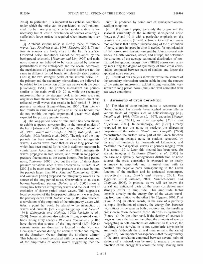
periods between 10 and 20 s (Figure 3). The cross correla-tions in this band exhibit a clear seasonal variation. Duringthe northern winter (October to March), the amplitude of thecausal part of the correlation is larger than the amplitude ofthe anticausal part. This indicates that most of the Rayleighwave energy propagates from MLAC to PHL (NE to SW).During the northern summer (May-September), the oppositeis observed: the noise is dominated by waves propagatingfrom PHL to MLAC (SW to NE). Moreover, during thewhole year, the Rayleigh waves are visible both at positiveand negative times. All this shows that in the period band ofthe primary microseism, an important contribution of thenoise observed in California is coming from the east, havinglikely its source in the Atlantic Ocean. The waveforms

Figure 1. Schematic illustration of the effect of inhomogeneous noise sources distribution on the degreeof symmetry of cross correlation. (a) Symmetric cross correlation between 1 and 2 obtained when thesources of noise are evenly distributed. (b) Asymmetric cross correlation (but symmetric travel times)associated with a nonisotropic distribution of sources.

B10306 STEHLY ET AL.: ORIGIN OF THE SEISMIC NOISE

3 of 12

B10306

observed at positive and negative times are not exactlyidentical because of the differences in the spectrum of thenoise coming from east or west.[10] To determine the main direction of the normalized

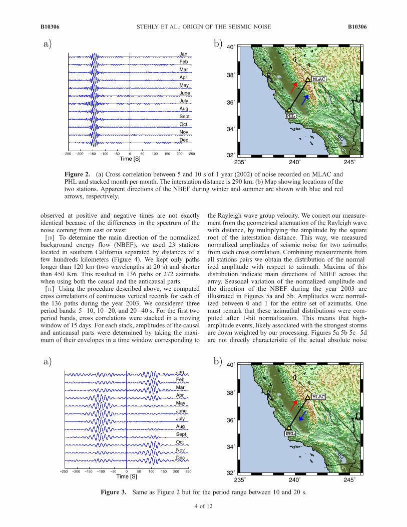
background energy flow (NBEF), we used 23 stationslocated in southern California separated by distances of afew hundreds kilometers (Figure 4). We kept only pathslonger than 120 km (two wavelengths at 20 s) and shorterthan 450 Km. This resulted in 136 paths or 272 azimuthswhen using both the causal and the anticausal parts.[11] Using the procedure described above, we computed

cross correlations of continuous vertical records for each ofthe 136 paths during the year 2003. We considered threeperiod bands: 5–10, 10–20, and 20–40 s. For the first twoperiod bands, cross correlations were stacked in a movingwindow of 15 days. For each stack, amplitudes of the causaland anticausal parts were determined by taking the maxi-mum of their envelopes in a time window corresponding to

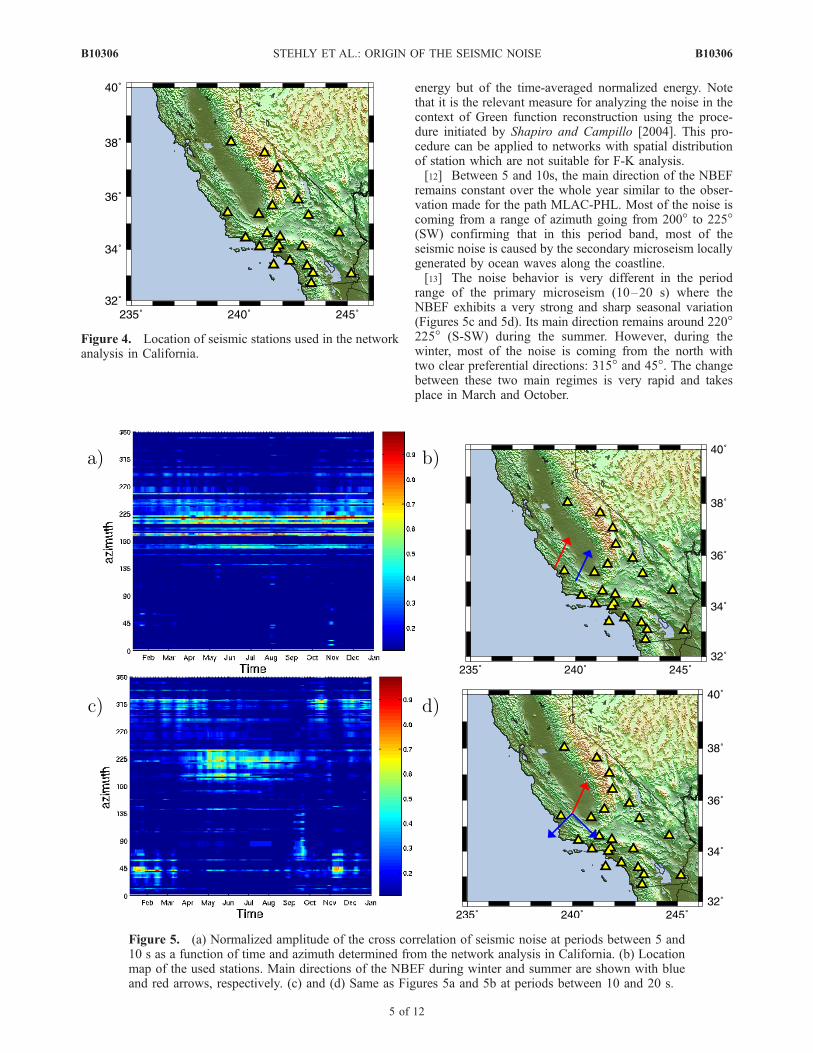
the Rayleigh wave group velocity. We correct our measure-ment from the geometrical attenuation of the Rayleigh wavewith distance, by multiplying the amplitude by the squareroot of the interstation distance. This way, we measurednormalized amplitudes of seismic noise for two azimuthsfrom each cross correlation. Combining measurements fromall stations pairs we obtain the distribution of the normal-ized amplitude with respect to azimuth. Maxima of thisdistribution indicate main directions of NBEF across thearray. Seasonal variation of the normalized amplitude andthe direction of the NBEF during the year 2003 areillustrated in Figures 5a and 5b. Amplitudes were normal-ized between 0 and 1 for the entire set of azimuths. Onemust remark that these azimuthal distributions were com-puted after 1-bit normalization. This means that high-amplitude events, likely associated with the strongest stormsare down weighted by our processing. Figures 5a 5b 5c–5dare not directly characteristic of the actual absolute noise

Figure 2. (a) Cross correlation between 5 and 10 s of 1 year (2002) of noise recorded on MLAC andPHL and stacked month per month. The interstation distance is 290 km. (b) Map showing locations of thetwo stations. Apparent directions of the NBEF during winter and summer are shown with blue and redarrows, respectively.

Figure 3. Same as Figure 2 but for the period range between 10 and 20 s.

B10306 STEHLY ET AL.: ORIGIN OF THE SEISMIC NOISE

4 of 12

B10306

energy but of the time-averaged normalized energy. Notethat it is the relevant measure for analyzing the noise in thecontext of Green function reconstruction using the proce-dure initiated by Shapiro and Campillo [2004]. This pro-cedure can be applied to networks with spatial distributionof station which are not suitable for F-K analysis.[12] Between 5 and 10s, the main direction of the NBEF

remains constant over the whole year similar to the obser-vation made for the path MLAC-PHL. Most of the noise iscoming from a range of azimuth going from 200� to 225�(SW) confirming that in this period band, most of theseismic noise is caused by the secondary microseism locallygenerated by ocean waves along the coastline.[13] The noise behavior is very different in the period

range of the primary microseism (10–20 s) where theNBEF exhibits a very strong and sharp seasonal variation(Figures 5c and 5d). Its main direction remains around 220�225� (S-SW) during the summer. However, during thewinter, most of the noise is coming from the north withtwo clear preferential directions: 315� and 45�. The changebetween these two main regimes is very rapid and takesplace in March and October.

Figure 4. Location of seismic stations used in the networkanalysis in California.

Figure 5. (a) Normalized amplitude of the cross correlation of seismic noise at periods between 5 and10 s as a function of time and azimuth determined from the network analysis in California. (b) Locationmap of the used stations. Main directions of the NBEF during winter and summer are shown with blueand red arrows, respectively. (c) and (d) Same as Figures 5a and 5b at periods between 10 and 20 s.

B10306 STEHLY ET AL.: ORIGIN OF THE SEISMIC NOISE

5 of 12

B10306

Figure 6. Normalized amplitude of the cross correlation averaged during (left) the winter and (right) thesummer versus azimuth for various frequency bands (a) 5–10 s, (b) 10–20 s, and (c) 20–40 s. The colorscale is the same as on Figure 5.

B10306 STEHLY ET AL.: ORIGIN OF THE SEISMIC NOISE

6 of 12

B10306

[14] This difference between the directions of NBEF ofthe primary and secondary microseisms is surprising be-cause it indicates that the two main spectral noise peaksobserved locally do not have the same region of origin. Thiscould be the result of the attenuation of the seismic waveswhich is stronger for shorter periods and cancels thecontributions of distant sources in the 5–10 s period band.Another explanation could be that the actual regions ofgeneration of the seismic noise is different in the differentperiod bands. This hypothesis is supported by the observa-tion that the azimuthal distribution is dominated in winterby a flux from azimuths between 180 and 225� for theperiod band 5–10 s while there is no significant contribu-tion from this directions for the period band 10 to 20 s.Before exploring further the origin of noise in the primarymicroseism band (10–20 s), let us consider longer period,i.e., the 20–40 s period band.[15] At longer periods, there is less scattering and we

expect the ambient seismic noise to be less diffuse. There-fore the reconstruction of Green functions requires averag-ing over longer time series. For this reason, we do notconsider anymore 15 days moving windows but analyze

longer time series by cross-correlating noise recorded eitherduring the winter (October to March) or the summer (Aprilto September). For these two periods, we measure normal-ized amplitudes of the Rayleigh wave part of the Greenfunction for the set of station pairs. Figure 6 shows theazimuthal distribution of the normalized amplitude of thecorrelation versus azimuth for the three different periodbands (5–10, 10–20, 20–40 s) during the winter (Figure 6,left) and the summer (Figure 6, right) of 2003.[16] While at periods between 5 and 10 s most of the

noise is coming from the coast during the whole year, thenoise provenance has a clear seasonal variability at longerperiods. Moreover, the normalized amplitude versus azi-muth diagrams for the 10–20 and 20–40 s period bandsexhibit main features which are similar, although notcompletely identical. Most of the background noise energyis coming from the northeast (possibly North Atlantic)during the winter and the main direction switches to thesouthwest during the summer. This similarity suggests thatthe average primary microseism may originate from thesame regions as the longer-period noise, which has beenconsidered to be excited by the infragravity ocean waves

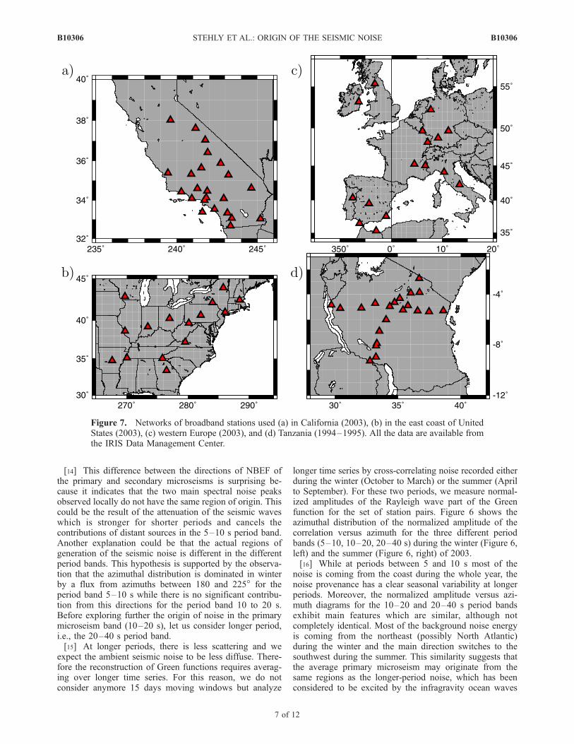
Figure 7. Networks of broadband stations used (a) in California (2003), (b) in the east coast of UnitedStates (2003), (c) western Europe (2003), and (d) Tanzania (1994–1995). All the data are available fromthe IRIS Data Management Center.

B10306 STEHLY ET AL.: ORIGIN OF THE SEISMIC NOISE

7 of 12

B10306

propagating away from the coast [Webb et al., 1991; Rhieand Romanowicz, 2004; Tanimoto, 2005]. We will investi-gate further the origin of the noise in the band of theprimary microseism by considering simultaneously severalnetworks.

4. Origin of the 10–20 s Noise

[17] Using the method described in section 3, we ana-lyzed the noise in several others regions of the world: eastcoast of United States, western Europe, and Tanzania(Figure 7). Similar to the Californian network, our analysisis based on the amplitudes of the reconstructed causal andanticausal Rayleigh waves. The data for the NorthernHemisphere are from 2003 and the Tanzanian data are from1994 to 1995, the period of the 97-005 PASSCAL exper-iment [Owens et al., 1997]. For each of these networks weestimated the normalized noise amplitudes as functions ofazimuth during the winter (October to March) and thesummer (April to September) for the period bands ofthe primary and the secondary microseisms. Similar to theobservations in California, the NBEF of the 5–10 s noiseremains stable over the whole year at all networks. Thisobservation is compatible with the idea that the generationof the secondary microseism is mostly controlled by the

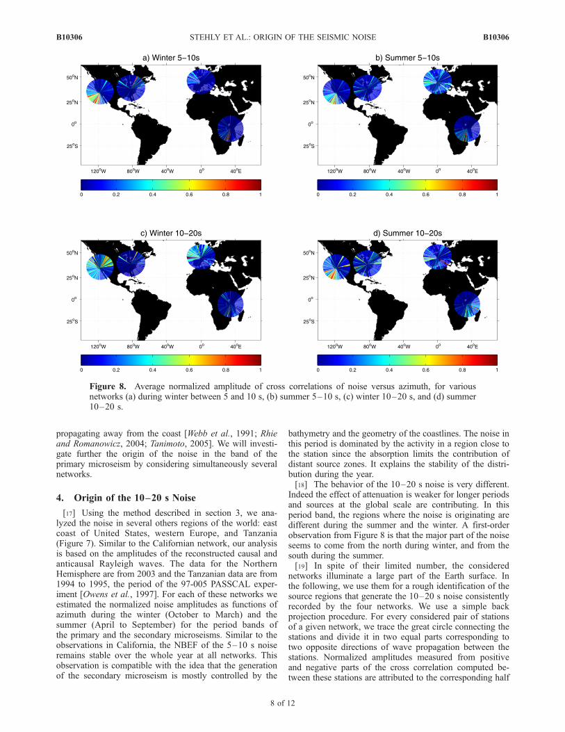
bathymetry and the geometry of the coastlines. The noise inthis period is dominated by the activity in a region close tothe station since the absorption limits the contribution ofdistant source zones. It explains the stability of the distri-bution during the year.[18] The behavior of the 10–20 s noise is very different.

Indeed the effect of attenuation is weaker for longer periodsand sources at the global scale are contributing. In thisperiod band, the regions where the noise is originating aredifferent during the summer and the winter. A first-orderobservation from Figure 8 is that the major part of the noiseseems to come from the north during winter, and from thesouth during the summer.[19] In spite of their limited number, the considered

networks illuminate a large part of the Earth surface. Inthe following, we use them for a rough identification of thesource regions that generate the 10–20 s noise consistentlyrecorded by the four networks. We use a simple backprojection procedure. For every considered pair of stationsof a given network, we trace the great circle connecting thestations and divide it in two equal parts corresponding totwo opposite directions of wave propagation between thestations. Normalized amplitudes measured from positiveand negative parts of the cross correlation computed be-tween these stations are attributed to the corresponding half

Figure 8. Average normalized amplitude of cross correlations of noise versus azimuth, for variousnetworks (a) during winter between 5 and 10 s, (b) summer 5–10 s, (c) winter 10–20 s, and (d) summer10–20 s.

B10306 STEHLY ET AL.: ORIGIN OF THE SEISMIC NOISE

8 of 12

B10306

great circle. This is an approximation since in the 10–20 speriod band the path followed by Rayleigh waves is notexactly a great circle because of the lateral heterogeneity ofthe crust and the mantle. We then define a 2� � 2� grid onthe surface of the Earth and take the mean value of thenormalized correlation amplitude associated with all greatcircles crossing every cell. To be able to use all fournetworks simultaneously, we assume that the seasonal noisevariability is stable over different years and combine the2003 data from the Northern Hemisphere with the 1994 datafrom Tanzania (results for individual networks are given inAppendix A).[20] The results for the four networks in the 10–20 s band

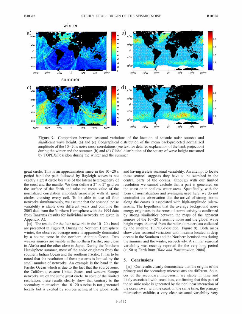
are presented in Figure 9. During the Northern Hemispherewinter, the observed average noise is apparently dominatedby a source zone in the northern Atlantic Ocean. Twoweaker sources are visible in the northern Pacific, one closeto Alaska and the other close to Japan. During the NorthernHemisphere summer, most of the noise originates from thesouthern Indian Ocean and the southern Pacific. It has to benoted that the resolution of these patterns is limited by thesmall number of networks. An example is the band in thePacific Ocean which is due to the fact that the source zone,the California, eastern United States, and western Europenetworks are on the same great circle. In spite of the limitedresolution, these results clearly show that contrary to thesecondary microseism, the 10–20 s noise is not generatedlocally but is excited by sources acting at the global scale

and having a clear seasonal variability. An attempt to locatethese sources suggests they have to be searched in thecentral parts of the oceans, although with our limitedresolution we cannot exclude that a part is generated onthe coast or in shallow water areas. Specifically, with theform of normalization and averaging used here, we do notcontradict the observation that the arrival of strong stormsalong the coasts is associated with high-amplitude micro-seisms. The hypothesis that the average background noiseenergy originates in the zones of storm activity is confirmedby strong similarities between the maps of the apparentsources of the 10–20 s seismic noise and the global waveheight maps obtained from the radar altimeter data collectedby the satellite TOPEX-Poseidon (Figure 9). Both mapsshow clear seasonal variations with maxima located in deepoceans in the Southern and the Northern hemispheres duringthe summer and the winter, respectively. A similar seasonalvariability was recently reported for the very long period(>150 s) Earth hum [Rhie and Romanowicz, 2004].

5. Conclusions

[21] Our results clearly demonstrate that the origins of theprimary and the secondary microseisms are different. Sour-ces of the secondary microseism are stable in time andlikely associated with coastlines, confirming that this part ofthe seismic noise is generated by the nonlinear interaction ofthe ocean swell with the coast. In the same time, the primarymicroseism exhibits a very clear seasonal variability very

Figure 9. Comparison between seasonal variations of the location of seismic noise sources andsignificant wave height. (a) and (c) Geographical distribution of the mean back-projected normalizedamplitude of the 10–20 s noise cross correlations (see text for detailed explanation of the back projection)during the winter and the summer. (b) and (d) Global distribution of the square of wave height measuredby TOPEX/Poseidon during the winter and the summer.

B10306 STEHLY ET AL.: ORIGIN OF THE SEISMIC NOISE

9 of 12

B10306

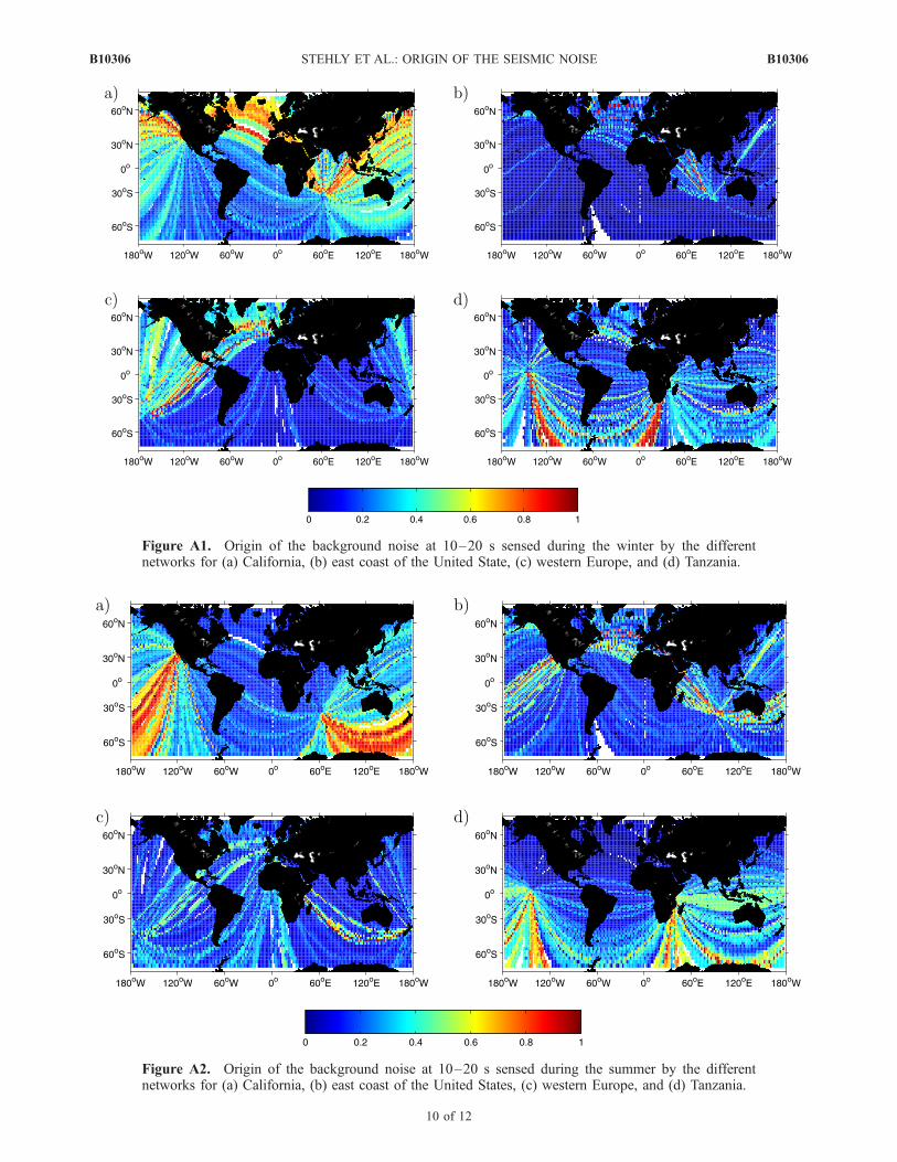
Figure A1. Origin of the background noise at 10–20 s sensed during the winter by the differentnetworks for (a) California, (b) east coast of the United State, (c) western Europe, and (d) Tanzania.

Figure A2. Origin of the background noise at 10–20 s sensed during the summer by the differentnetworks for (a) California, (b) east coast of the United States, (c) western Europe, and (d) Tanzania.

B10306 STEHLY ET AL.: ORIGIN OF THE SEISMIC NOISE

10 of 12

B10306

similar to the behavior of the long-period noise suggestingthat the seismic noise for periods larger than 10 s isproduced by a single mechanism not directly related tothe action of the swell on the coast. This hypothesis is alsofavored by the good correlation between the distributions ofthe seismic noise sources determined from the networkanalysis with the maps of average ocean wave height mapobtained by TOPEX-Poseidon.[22] This seasonal variation also means that the quality of

the Green function reconstruction by cross-correlation canbe different with noise recorded during the summer andduring the winter. Using simultaneously data recordedduring the winter and the summer would be a way toincrease the number of high-quality measurements and toimprove the resolution of seismic imaging based on noisecross correlation.[23] The long-period seismic noise is likely produced

by the infragravity waves [Webb et al., 1991; Rhie andRomanowicz, 2004; Tanimoto, 2005]. According to Webb etal. [1991], long-period gravity waves propagate freely awayfrom the coast lines. Recent observations indicate that thespectrum of this class of waves can be extended to relativelyshort periods (�20 s) [Dolenc et al., 2005]. FollowingLonguet-Higgins [1950], bottom pressure fluctuations arisefrom the interaction of swells propagating in oppositedirections. Although the most commonly considered con-figuration to encounter such a system of waves involves thereflection of the swell from the coast, it can also begenerated in the area of strong storm activity even in deepoceans. Others sources of pressure fluctuations in deepwater can be associated with the interaction of propagatingswell of slightly different frequencies with high amplitudecurrents [Longuet-Higgings and Stewart, 1964]. These

kinds of mechanisms of generation are compatible withthe location of background noise source regions in the zonesof highest sea waves.

Appendix A

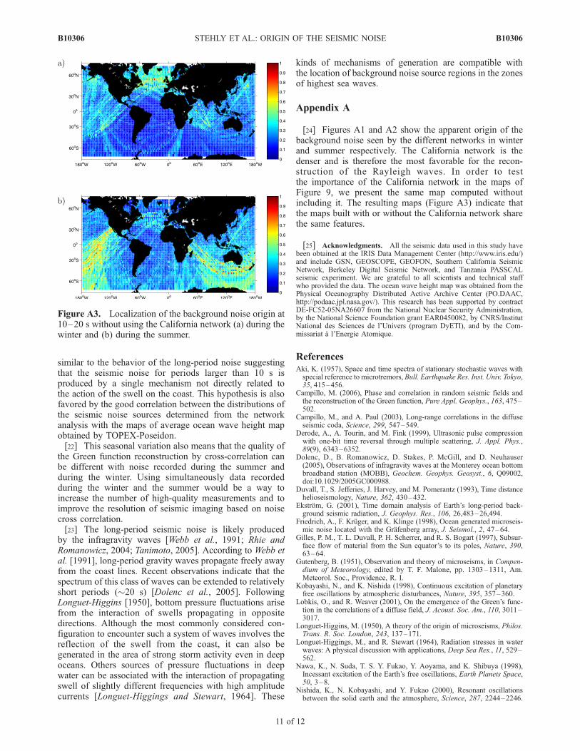
[24] Figures A1 and A2 show the apparent origin of thebackground noise seen by the different networks in winterand summer respectively. The California network is thedenser and is therefore the most favorable for the recon-struction of the Rayleigh waves. In order to testthe importance of the California network in the maps ofFigure 9, we present the same map computed withoutincluding it. The resulting maps (Figure A3) indicate thatthe maps built with or without the California network sharethe same features.

[25] Acknowledgments. All the seismic data used in this study havebeen obtained at the IRIS Data Management Center (http://www.iris.edu/)and include GSN, GEOSCOPE, GEOFON, Southern California SeismicNetwork, Berkeley Digital Seismic Network, and Tanzania PASSCALseismic experiment. We are grateful to all scientists and technical staffwho provided the data. The ocean wave height map was obtained from thePhysical Oceanography Distributed Active Archive Center (PO.DAAC,http://podaac.jpl.nasa.gov/). This research has been supported by contractDE-FC52-05NA26607 from the National Nuclear Security Administration,by the National Science Foundation grant EAR0450082, by CNRS/InstitutNational des Sciences de l’Univers (program DyETI), and by the Com-missariat a l’Energie Atomique.

ReferencesAki, K. (1957), Space and time spectra of stationary stochastic waves withspecial reference to microtremors, Bull. Earthquake Res. Inst. Univ. Tokyo,35, 415–456.

Campillo, M. (2006), Phase and correlation in random seismic fields andthe reconstruction of the Green function, Pure Appl. Geophys., 163, 475–502.

Campillo, M., and A. Paul (2003), Long-range correlations in the diffuseseismic coda, Science, 299, 547–549.

Derode, A., A. Tourin, and M. Fink (1999), Ultrasonic pulse compressionwith one-bit time reversal through multiple scattering, J. Appl. Phys.,89(9), 6343–6352.

Dolenc, D., B. Romanowicz, D. Stakes, P. McGill, and D. Neuhauser(2005), Observations of infragravity waves at the Monterey ocean bottombroadband station (MOBB), Geochem. Geophys. Geosyst., 6, Q09002,doi:10.1029/2005GC000988.

Duvall, T., S. Jefferies, J. Harvey, and M. Pomerantz (1993), Time distancehelioseismology, Nature, 362, 430–432.

Ekstrom, G. (2001), Time domain analysis of Earth’s long-period back-ground seismic radiation, J. Geophys. Res., 106, 26,483–26,494.

Friedrich, A., F. Kruger, and K. Klinge (1998), Ocean generated microseis-mic noise located with the Grafenberg array, J. Seismol., 2, 47–64.

Gilles, P. M., T. L. Duvall, P. H. Scherrer, and R. S. Bogart (1997), Subsur-face flow of material from the Sun equator’s to its poles, Nature, 390,63–64.

Gutenberg, B. (1951), Observation and theory of microseisms, in Compen-dium of Meteorology, edited by T. F. Malone, pp. 1303–1311, Am.Meteorol. Soc., Providence, R. I.

Kobayashi, N., and K. Nishida (1998), Continuous excitation of planetaryfree oscillations by atmospheric disturbances, Nature, 395, 357–360.

Lobkis, O., and R. Weaver (2001), On the emergence of the Green’s func-tion in the correlations of a diffuse field, J. Acoust. Soc. Am., 110, 3011–3017.

Longuet-Higgins, M. (1950), A theory of the origin of microseisms, Philos.Trans. R. Soc. London, 243, 137–171.

Longuet-Higgings, M., and R. Stewart (1964), Radiation stresses in waterwaves: A physical discussion with applications, Deep Sea Res., 11, 529–562.

Nawa, K., N. Suda, T. S. Y. Fukao, Y. Aoyama, and K. Shibuya (1998),Incessant excitation of the Earth’s free oscillations, Earth Planets Space,50, 3–8.

Nishida, K., N. Kobayashi, and Y. Fukao (2000), Resonant oscillationsbetween the solid earth and the atmosphere, Science, 287, 2244–2246.

Figure A3. Localization of the background noise origin at10–20 s without using the California network (a) during thewinter and (b) during the summer.

B10306 STEHLY ET AL.: ORIGIN OF THE SEISMIC NOISE

11 of 12

B10306

Owens, T., H. Crotwell, A. Nyblade, R. Brazier, and C. Langston (1997),PASSCAL data report 97005, IRIS Data Manage. Center, Washington,D. C.

Paul, A., M. Campillo, L. Margerin, E. Larose, and A. Derode (2005),Empirical synthesis of time-asymmetrical Green functions from the cor-relation of coda waves, J. Geophys. Res., 110, B08302, doi:10.1029/2004JB003521.

Pederson, H., F. Kruger, and the SVEKALAPKO Seismic TomographyWorking Group (2006), Influence of the seismic noise characteristicson noise correlations in the baltic shield, Geophys. J. Int, in press.

Rhie, J., and B. Romanowicz (2004), Excitation of Earth’s continuous freeoscillations by atmosphere-ocean-seafloor couplinng, Nature, 431, 552–554.

Roult, G., and W. Crawford (2000), Analysis of ‘backgrounds’ oscillationsand how to improve resolution by subtracting the atmospheric pressuresignal, Phys. Earth Planet. Inter, 121, 325–338.

Roux, P., and W. A. Kuperman (2003), Extracting coherent wavefrontsfrom acoustic ambient noise in the ocean, J. Acoust. Soc. Am, 116,1995–2003.

Sabra, K. G., P. Gerstoft, P. Roux, W. A. Kuperman, and M. C. Fehler(2005a), Surface wave tomography from microseisms in Southern Cali-fornia, Geophys. Res. Lett., 32, L14311, doi:10.1029/2005GL023155.

Sabra, K. G., P. Gerstoft, P. Roux, W. A. Kuperman, and M. C. Fehler(2005b), Surface wave tomography from microseisms in Southern Cali-fornia, Geophys. Res. Lett., 32, L14311, doi:10.1029/2005GL023155.

Sanchez-Sesma, F., and M. Campillo (2006), Retrieval of the green functionfrom cross correlation: The canonical elastic problem, Bull. Seismol. Soc.Am., 96(3), 1182–1191, doi:10.1785/0120050181.

Schulte-Pelkum, V., P. S. Earle, and F. L. Vernon (2004), Strong directivityof ocean-generated seismic noise, Geochem. Geophys. Geosyst., 5,Q03004, doi:10.1029/2003GC000520.

Shapiro, N. M., and M. Campillo (2004), Emergence of broadband Ray-leigh waves from correlations of the ambient seismic noise, Geophys.Res. Lett., 31, L07614, doi:10.1029/2004GL019491.

Shapiro, N., M. Campillo, L. Stehly, and M. Ritzwoller (2005), High-re-solution surface wave tomography from ambient seismic noise, Science,307, 1615–1618.

Snieder, R. (2004), Extracting the green’s function from the correlation ofcoda waves: A derivation based on stationary phase, Phys. Rev. E, 69.

Suda, N., K. Nawa, and Y. Fukao (1998), Earth’s background free oscilla-tions, Science, 279, 2089–2091.

Tanimoto, T. (2005), The oceanic excitation hypothesis for the continuousoscillations of the Earth, Geophys. J. Int, 160, 276–288.

Tanimoto, T., and J. Um (1999), Cause of continuous oscillations of theearth, J. Geophys. Res., 104(B12), 723–739.

Tanimoto, T., J. Um, K. Nishida, and N. Kobayashi (1998), Earth’s con-tinuous oscillations observed seismically quiet days, Geophys. Res. Lett.,25, 1553–1556.

Van Tiggelen, B. (2003), Green function retrieval and time reversal in adisordered world, Phys. Rev. Lett, 91(24), 243904.

Watada, S., A. Kobayashi, and E. Fujita (2001), Seasonal variations ofatmospheric and ocean-bottom pressure data in millihertz band, paperpresented at OHP/ION Joint Symposium’ Long-Term Observations inthe Oceans, Earthquake Res. Inst., Univ. of Tokyo, Mt. Fuji, Japan.

Weaver, R. L., and O. I. Lobkis (2001), Ultrasonics without a source:Thermal fluctuation correlation at MHz frequencies, Phys. Rev. Lett.,87(13).

Webb, S., X. Zhang, and W. Crawford (1991), Infragravity waves in thedeep ocean, J. Geophys. Res., 96, 2723–2736.

�����������������������M. Campillo and L. Stehly, Universite Joseph Fourier, CNRS, LGIT, BP

53, F-38041 Grenoble, France. (lstehly@obs.ujf-grenoble.fr)N. M. Shapiro, Laboratoire de Sismologie, IPGP, CNRS, 5 place Jussieu,

F-75005 Paris, France.

B10306 STEHLY ET AL.: ORIGIN OF THE SEISMIC NOISE

12 of 12

B10306