A Study of the Long Term Evolution in Active

Region Upflows

Louise K. HARRA1∗, Ignacio UGARTE-URRA,2 , Marc DE ROSA,3, Cristina

MANDRINI4 , Lidia VAN DRIEL-GESZTELYI1,5 , Deborah BAKER1, J. Leonard

CULHANE1 and Pascal DEMOULIN5

1UCL-Mullard Space Science Laboratory, Holmbury St Mary, Dorking, Surrey, RH5 6NT, UK

2Space Science Division, Code 7681, Naval Research Laboratory, Washington, DC 20375,

USA

3Lockheed Martin Solar and Astrophysics Laboratory, 3251 Hanover St. B/252, Palo Alto, CA

94304,, USA

4Instituto de Astronoma y Fsica del Espacio (IAFE), UBA-CONICET, CC. 67, Suc. 28 Buenos

Aires, 1428, Argentina

5Observatoire de Paris, LESIA, UMR 8109 (CNRS), 92195, Meudon Principal Cedex, France

∗E-mail: l.harra@ucl.ac.uk, ignacio.ugarte-urra@nrl.navy.mil, derosa@lmsal.com, mandrini@iafe.uba.ar,

Lidia.VanDriel@obspm.fr, deborah.baker@ucl.ac.uk, j.culhane@ucl.ac.uk, Pascal.Demoulin@obspm.fr

Received ; Accepted

Abstract

Since their discovery, upflows at the edges of active regions have attracted a lot of interest

primarily as they potentially could contribute to the slow solar wind. One aspect that has not

been studied yet is how the long term evolution of active regions impacts the upflows. In this

work, we analyse one active region that survives three solar rotations. We track how the flows

change with time. We use local and global modelling of the decaying active region to determine

how the age of the active region will impact the extent of the open magnetic fields then how

some of the upflows could become outflows. We finish with a discussion of how these results,

set in a broader context, can be further developed with the Solar Orbiter mission.

1

Key words: Sun: corona, Sun: magnetic fields, Sun: evolution

1 Introduction

This paper is developed following the 10th Hinode Science meeting in Nagoya, celebrating 10 years

of successful operations of the mission. In the first decade one of the first, and most significant

results from the mission, was that of upflowing plasma being observed consistently at the edges of

active regions on the Sun. The first example published with Hinode data was by Sakao et al. (2007)

using both the X-ray telescope (XRT) data and the EUV imaging spectrometer (EIS) data. The active

region was observed to be close to a coronal hole, and persistent flowing plasma was seen reaching

speeds of over 100 km s−1 in fan-like structures at the edges of the region. The plasma was confirmed

to be a true upflow using the spatially resolved spectroscopic data from EIS (Harra et al. (2008).

Doschek et al. (2008)) determined the physical plasma parameters in these regions, and found a

positive correlation between the Doppler velocity and the non-thermal velocity indicating a spread

of velocities. Hara et al. (2008) explored this further and found deviation from a single-Gaussian

profile, indicating unresolved high-speed flows exist. The cadence of these flows was analysed by

Ugarte-Urra and Warren (2011) who found that they vary on timescales as short as the 5-min that was

used in the study. This all indicates a highly dynamical region that is capable of producing fast flows.

These dynamic flows are a persistent feature and are seen in most if not all active regions, and have

been tracked for long periods (e.g. Baker et al. 2017; Zangrilli and Poletto 2016).

Although fast flows are clearly measured, it is hard to determine if they actually do leave the

Sun to form part of the slow solar wind. The difficulties are due to the small field of view of the spec-

troscopy measurements combined with the distance travelled before the solar wind is measured in situ

(1 au). This distance allows for expansion and interaction with pre-existing winds of different speeds

confusing the picture. One way to confirm that upflows can form part of the slow solar wind is to mea-

sure the chemical abundance. Brooks and Warren (2011) compared the composition of the upflows

seen with EIS with those measured in situ and found them to be comparable. Full Sun observations

with EIS revealed several potential active region sources of the slow solar wind at one time (Brooks

et al. 2015). Not all of the upflows originating from these sources will necessarily make it into the

solar wind. Magnetic modeling is another tool to examine whether or not upflows become outflows

∗

2

and part of the solar wind. van Driel-Gesztelyi et al. (2012) were the first to follow the pathway of

upflows from the edge of an active region to an intermediate-speed solar wind stream, establishing

the link via a high-altitude null-point in an open-field domain where magnetic reconnection between

active region loops and field lines open towards the heliosphere channeled active-region plasma into

the solar wind. The combination of detailed analysis of the coronal data, the magnetic field modeling

of the studied AR and of the large scales, its topology, as well as the solar wind properties, in partic-

ular its plasma composition, are required to find enough clues to associate particular upflows to some

in situ solar wind measurements (Culhane et al. 2014; Mandrini et al. 2014).

The previous works tend to use single case examples. Recently Edwards et al. (2016) studied

seven active regions, combining observations and modelling to determine whether the upflows have a

route to escape into the slow wind. It was found in most cases that the upflows are not from a region

where there is open magnetic field which allows them a route into the wind. Often the upflows are

the footpoints of large extended loops. Recent work by Fazakerley et al. (2016) has tracked a full

Carrington rotation and analysed the active region outflows and the slow solar wind behaviour during

that time. In locations where active regions are situated beside coronal holes there was enhanced

intermediate solar wind velocity, suggesting that location is key. Zangrilli and Poletto (2016) have

analysed data combined with PFSS modelling for a single active region over its lifetime at the limb

with SOHO/UVCS data, and found that throughout its lifetime of five rotations it was possible to

measure outflows in the intermediate corona.

In this work, we focus on the active region on the disk, and ask the question, ’how do the

upflows change during the decay of an active region?’. We look at an active region over several

rotations and apply both local and global modelling to understand its evolution. We summarise the

paper by looking towards the Solar Orbiter mission, the main goal of which is to observe the solar

wind within 0.3 au of the Sun.

2 Data Analysis

We analysed a decaying active region over three rotations, using data from three space missions, as

described below.

2.1 Hinode EUV Imaging Spectrometer (EIS)

The Hinode/EIS (Culhane et al. 2007) is a scanning slit spectrometer observing in two wave bands in

the EUV: 170–210 A and 250–290 A. The spectral resolution is 0.0223 A pixel−1, which allows ve-

locity measurements of a few km s−1. The standard calibration was used through the routine eis prep.

3

Additionally, the slit tilt and the orbital variation of line position were corrected. For each pixel we

fitted the line using a single Gaussian profile producing an intensity and Doppler-velocity ‘image’

for each raster scan. We concentrated on the Fe XII emission line as it is the strongest line and was

observed in all the studies for each rotation. The errors on the spectral line fits were up to 3 km s−1 .

2.2 SDO: Atmospheric Imaging Assembly (AIA)

SDO/AIA (Lemen et al. 2012) observes the Sun in seven EUV and three UV channels with a pixel

size of 0.6′′ and a time cadence of 12 s for each EUV channel and 24s for each UV channel. AIA data

were analysed in the 193 A channel so that they could be co-aligned with the EIS 195 A data easily,

and the evolution of the active regions studied.

2.3 SDO: Helioseismic and Magnetic Imager (HMI)

SDO/HMI (Scherrer et al. 2012) is designed to observe magnetic field and oscillations at the solar

surface with a spatial resolution of 1′′. For this work, we used the line-of-sight component magnetic

field measurements that are collected every 45 seconds.

2.4 STEREO: Extreme Ultraviolet Imager (EUVI)

The twin STEREO spacecraft (Kaiser et al. 2008) provide two observational vantage points of the

Sun. We used near-simultaneous images from STEREO/EUVI (Howard et al. 2008) and SDO/AIA

to construct full-Sun heliographic maps of the Sun that allowed us to track the evolution of active

regions over several rotations (e.g. Ugarte-Urra et al. 2015) and identify a suitable dataset.

3 The decaying active region

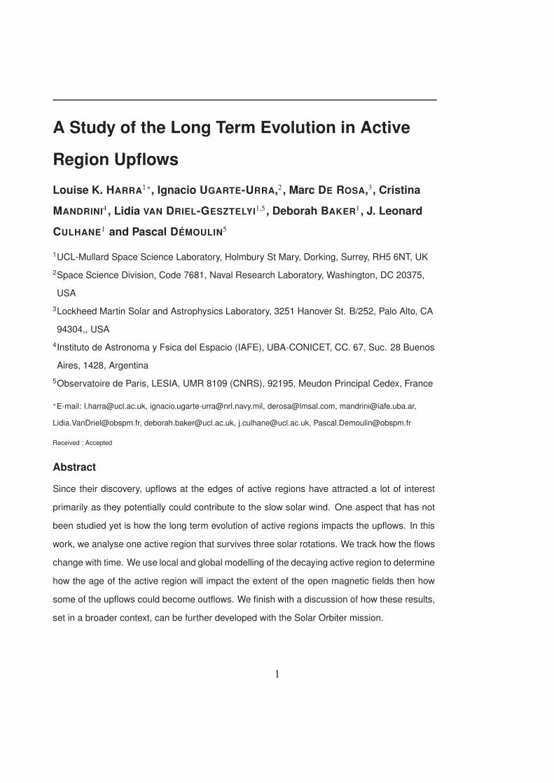
These observations follow the process of a decaying active region throughout the three rotations

without too much of an interruption from new emerging magnetic flux. This active region was initially

designated as AR11532 by NOAA on its first rotation in early August 2012. Figure 1 shows the line

of sight magnetic field as observed by HMI, and also the resulting coronal structure as observed by

AIA 193 A. The active region emerged on the far side and rotated on the solar disc as a mature active

region. It consisted of two bipoles with the smaller one cancelling during the first rotation. During the

second rotation, now designated as AR11553, the region was undergoing decay whilst maintaining

its leading spot. There was some further small flux emergence during this rotation. In rotation three,

the leading spot had decayed, and there was no major flux emergence occurring in the region, now

called, AR11576. The active region was one of the few ‘classic’ examples of an isolated decaying

4

Fig. 1. The top row shows the line of sight magnetic field from HMI for 3 rotations of the same active region. The lower plots show the images in the 193 A

band of AIA.

active region for which Hinode/EIS data were available in multiple rotations.

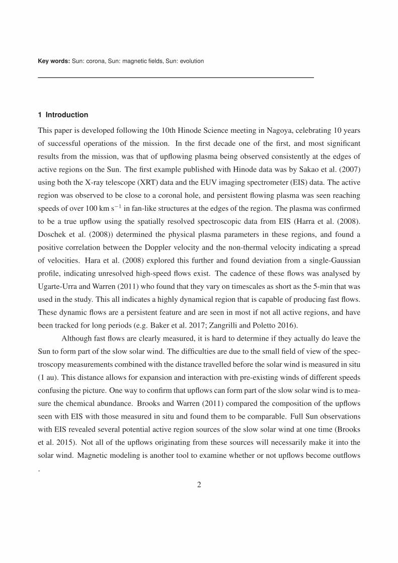
We analysed EIS data in each rotation to study the location of the upflows. The EIS field of

view is not large enough to cover the extents of both polarities, so in this example we concentrate

on the western side. In the first rotation the available raster was not at disk centre which may be

problematic for Doppler flow measurements because of line-of-sight effects (described in Demoulin

et al. 2013). However as can be seen in Figure 2, the western side of the active region shows upflows

at each rotation. The upflows on the western side become more extended by rotation 3, and indeed

are directed both north and south. In the previous two rotations, the upflows were dominantly in the

northwards direction. The change appears to come about due to the dispersed magnetic field and

disappearance of the sunspot. The upflows measured do not necessarily become outflows, and can be

associated with expanding loops or open field.

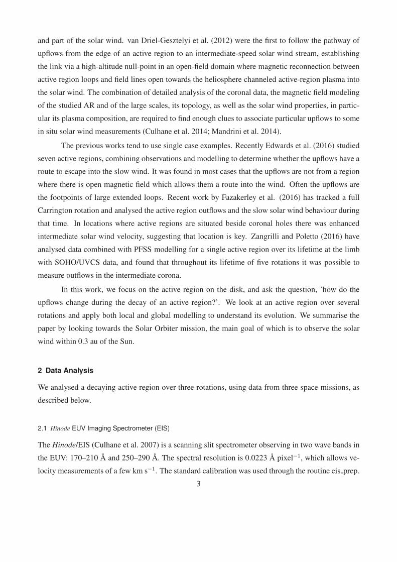
In order to understand the change in the upflows in more detail, we plotted histograms of

the Doppler shifts on the western side for each rotation in Figure 3. Rotation 3, which is when the

magnetic field is very dispersed and there is no sunspot, shows that more pixels are showing blue-

shifted velocities than rotation 2. The number of blue-shifted pixels significantly increased (by 50%)

between rotations 2 and 3, with rotation 2 having 1280 pixels with blue-shifted values versus 1916

pixels in rotation 3. In addition to the bulk flows, we also looked at the line width of the Fe XII

line profile through measurement of the non-thermal velocity. As discussed in the Introduction, non-

thermal velocities can provide an indication of the spread of velocities. The number of pixels with

higher non-thermal velocities significantly increases for rotation 3 as can be seen in Figure 3. This

5

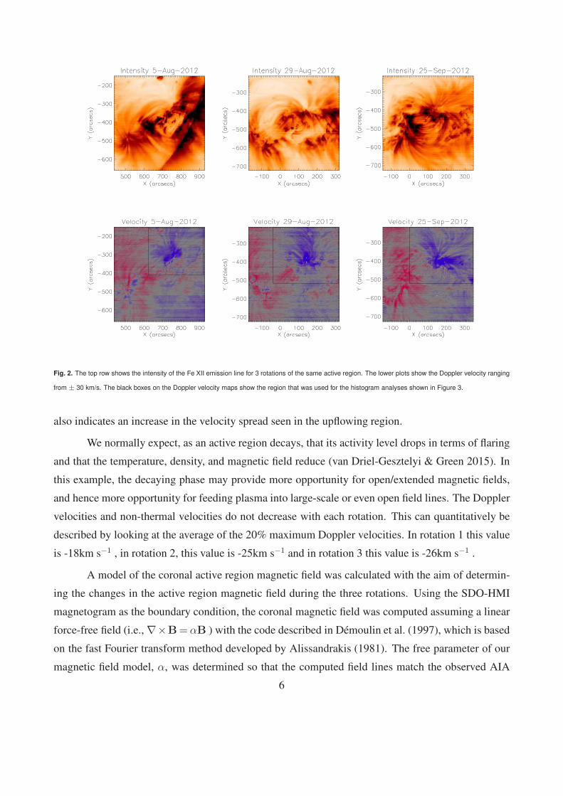
Fig. 2. The top row shows the intensity of the Fe XII emission line for 3 rotations of the same active region. The lower plots show the Doppler velocity ranging

from ± 30 km/s. The black boxes on the Doppler velocity maps show the region that was used for the histogram analyses shown in Figure 3.

also indicates an increase in the velocity spread seen in the upflowing region.

We normally expect, as an active region decays, that its activity level drops in terms of flaring

and that the temperature, density, and magnetic field reduce (van Driel-Gesztelyi & Green 2015). In

this example, the decaying phase may provide more opportunity for open/extended magnetic fields,

and hence more opportunity for feeding plasma into large-scale or even open field lines. The Doppler

velocities and non-thermal velocities do not decrease with each rotation. This can quantitatively be

described by looking at the average of the 20% maximum Doppler velocities. In rotation 1 this value

is -18km s−1 , in rotation 2, this value is -25km s−1 and in rotation 3 this value is -26km s−1 .

A model of the coronal active region magnetic field was calculated with the aim of determin-

ing the changes in the active region magnetic field during the three rotations. Using the SDO-HMI

magnetogram as the boundary condition, the coronal magnetic field was computed assuming a linear

force-free field (i.e., ∇×B= αB ) with the code described in Demoulin et al. (1997), which is based

on the fast Fourier transform method developed by Alissandrakis (1981). The free parameter of our

magnetic field model, α, was determined so that the computed field lines match the observed AIA

6

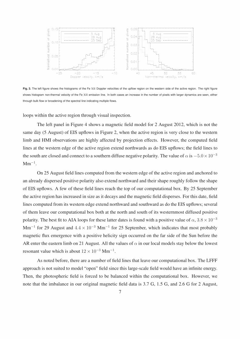
Fig. 3. The left figure shows the histograms of the Fe XII Doppler velocities of the upflow region on the western side of the active region. The right figure

shows histogram non-thermal velocity of the Fe XII emission line. In both cases an increase in the number of pixels with larger dynamics are seen, either

through bulk flow or broadening of the spectral line indicating multiple flows.

loops within the active region through visual inspection.

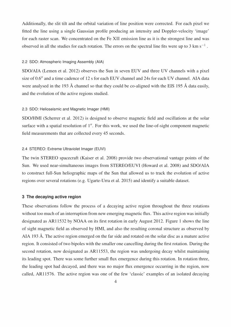
The left panel in Figure 4 shows a magnetic field model for 2 August 2012, which is not the

same day (5 August) of EIS upflows in Figure 2, when the active region is very close to the western

limb and HMI observations are highly affected by projection effects. However, the computed field

lines at the western edge of the active region extend northwards as do EIS upflows; the field lines to

the south are closed and connect to a southern diffuse negative polarity. The value of α is −5.0×10−3

Mm−1.

On 25 August field lines computed from the western edge of the active region and anchored to

an already dispersed positive polarity also extend northward and their shape roughly follow the shape

of EIS upflows. A few of these field lines reach the top of our computational box. By 25 September

the active region has increased in size as it decays and the magnetic field disperses. For this date, field

lines computed from its western edge extend northward and southward as do the EIS upflows; several

of them leave our computational box both at the north and south of its westernmost diffused positive

polarity. The best fit to AIA loops for these latter dates is found with a positive value of α, 3.8×10−3

Mm−1 for 29 August and 4.4× 10−3 Mm−1 for 25 September, which indicates that most probably

magnetic flux emergence with a positive helicity sign occurred on the far side of the Sun before the

AR enter the eastern limb on 21 August. All the values of α in our local models stay below the lowest

resonant value which is about 12× 10−3 Mm−1.

As noted before, there are a number of field lines that leave our computational box. The LFFF

approach is not suited to model “open” field since this large-scale field would have an infinite energy.

Then, the photospheric field is forced to be balanced within the computational box. However, we

note that the imbalance in our original magnetic field data is 3.7 G, 1.5 G, and 2.6 G for 2 August,

7

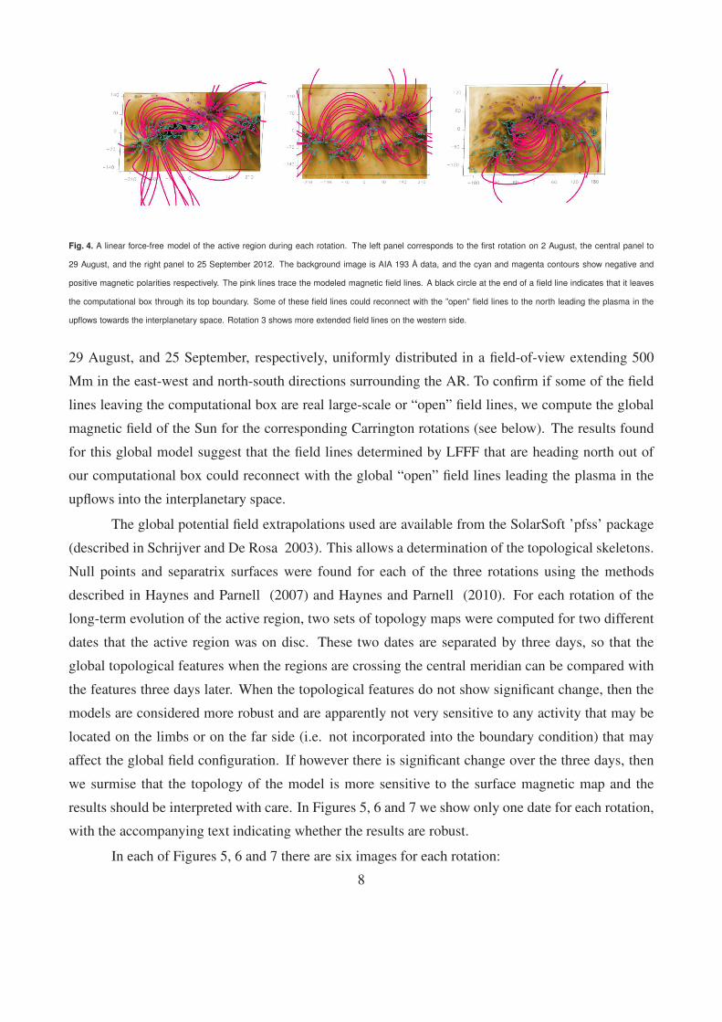
Fig. 4. A linear force-free model of the active region during each rotation. The left panel corresponds to the first rotation on 2 August, the central panel to

29 August, and the right panel to 25 September 2012. The background image is AIA 193 A data, and the cyan and magenta contours show negative and

positive magnetic polarities respectively. The pink lines trace the modeled magnetic field lines. A black circle at the end of a field line indicates that it leaves

the computational box through its top boundary. Some of these field lines could reconnect with the ”open” field lines to the north leading the plasma in the

upflows towards the interplanetary space. Rotation 3 shows more extended field lines on the western side.

29 August, and 25 September, respectively, uniformly distributed in a field-of-view extending 500

Mm in the east-west and north-south directions surrounding the AR. To confirm if some of the field

lines leaving the computational box are real large-scale or “open” field lines, we compute the global

magnetic field of the Sun for the corresponding Carrington rotations (see below). The results found

for this global model suggest that the field lines determined by LFFF that are heading north out of

our computational box could reconnect with the global “open” field lines leading the plasma in the

upflows into the interplanetary space.

The global potential field extrapolations used are available from the SolarSoft ’pfss’ package

(described in Schrijver and De Rosa 2003). This allows a determination of the topological skeletons.

Null points and separatrix surfaces were found for each of the three rotations using the methods

described in Haynes and Parnell (2007) and Haynes and Parnell (2010). For each rotation of the

long-term evolution of the active region, two sets of topology maps were computed for two different

dates that the active region was on disc. These two dates are separated by three days, so that the

global topological features when the regions are crossing the central meridian can be compared with

the features three days later. When the topological features do not show significant change, then the

models are considered more robust and are apparently not very sensitive to any activity that may be

located on the limbs or on the far side (i.e. not incorporated into the boundary condition) that may

affect the global field configuration. If however there is significant change over the three days, then

we surmise that the topology of the model is more sensitive to the surface magnetic map and the

results should be interpreted with care. In Figures 5, 6 and 7 we show only one date for each rotation,

with the accompanying text indicating whether the results are robust.

In each of Figures 5, 6 and 7 there are six images for each rotation:

8

Fig. 5. Global topological models of AR 11532 (the first rotation). The AR is indicated by a conical cyan pointer (a) magnetogram (b) open field locations with

the polarities (black=negative, white=positive) indicated (c) open field location with open field lines overlaid (green) (d) separatrix surfaces in the model, (e)

same as (d) but rotated so that the AR of interest is located at disk center, and (f) same as (d) but with the selection of open fieldlines in (c) included in the

rendering. With the exception of panel (e), the viewpoint for all models is that of an observer positioned along the Earth-Sun line.

(a) an orthographic projection of the surface magnetic map;

(b) a trinary image showing the photospheric footpoints of open flux, as determined from the global

model, with color (black/white) indicating polarity of the open field (negative/positive);

(c) a trinary image showing the photospheric footpoints of open flux, as determined from the global

model, with color (black/white) indicating polarity of the open field (negative/positive) plus open

field lines overlaid in green;

(d) separatrix surfaces in the model,

(e) same as (d) but rotated so that the AR of interest is located at disk center,

(f) same as (d) but with the selection of open fieldlines in (c) included in the rendering.

With the exception of panel (e), the viewpoint for all models is that of an observer positioned

along the Earth-Sun line for the date indicated.

In the images of Figure 5, 6 and 7 that show the field topology, each null point is depicted as

a (barely visible) small red dot. Extending out of each null point is a spine fieldline (cyan) and its

associated separatrix surface (shown in various pastel colours). The edges of these separatrix surfaces

9

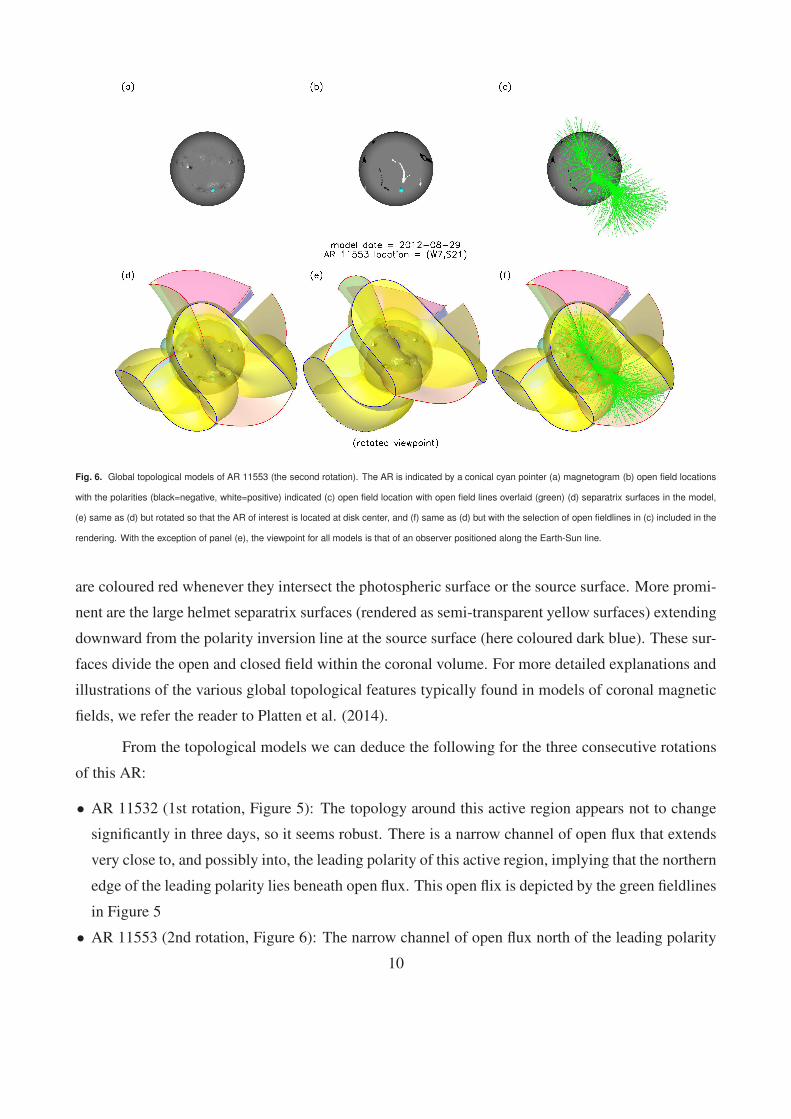
Fig. 6. Global topological models of AR 11553 (the second rotation). The AR is indicated by a conical cyan pointer (a) magnetogram (b) open field locations

with the polarities (black=negative, white=positive) indicated (c) open field location with open field lines overlaid (green) (d) separatrix surfaces in the model,

(e) same as (d) but rotated so that the AR of interest is located at disk center, and (f) same as (d) but with the selection of open fieldlines in (c) included in the

rendering. With the exception of panel (e), the viewpoint for all models is that of an observer positioned along the Earth-Sun line.

are coloured red whenever they intersect the photospheric surface or the source surface. More promi-

nent are the large helmet separatrix surfaces (rendered as semi-transparent yellow surfaces) extending

downward from the polarity inversion line at the source surface (here coloured dark blue). These sur-

faces divide the open and closed field within the coronal volume. For more detailed explanations and

illustrations of the various global topological features typically found in models of coronal magnetic

fields, we refer the reader to Platten et al. (2014).

From the topological models we can deduce the following for the three consecutive rotations

of this AR:

• AR 11532 (1st rotation, Figure 5): The topology around this active region appears not to change

significantly in three days, so it seems robust. There is a narrow channel of open flux that extends

very close to, and possibly into, the leading polarity of this active region, implying that the northern

edge of the leading polarity lies beneath open flux. This open flix is depicted by the green fieldlines

in Figure 5

• AR 11553 (2nd rotation, Figure 6): The narrow channel of open flux north of the leading polarity

10

Fig. 7. Global topological models of AR 11576 (the third rotation). The AR is indicated by a conical cyan pointer (a) magnetogram (b) open field locations

with the polarities (black=negative, white=positive) indicated (c) open field location with open field lines overlaid (green) (d) separatrix surfaces in the model,

(e) same as (d) but rotated so that the AR of interest is located at disk center, and (f) same as (d) but with the selection of open fieldlines in (c) included in the

rendering. With the exception of panel (e), the viewpoint for all models is that of an observer positioned along the Earth-Sun line.

of this AR evident in the first rotation remains, with little apparent change in its area. As with the

previous rotation, the topology around this active region appears not to change much in three days,

so the model seems to be robust. The leading polarity appears to lie beneath open flux.

• AR 11576 (3rd rotation, Figure 7): The topology is found to differ significantly between the two

dates sampled, 25-09-2012 and 28-09-2012, and therefore the conclusions drawn from these topol-

ogy renderings are much more uncertain. We find that the topology from 25-09-2012 does have a

narrow channel of open flux to the north and west of the target region that is similar to the narrow

channels evident in the previous rotations. The current-sheet structure is more complex (in fact,

two current sheets are evident), owing to the fact that the axial dipole is in the process of reversing

sign, which allows higher-degree harmonic modes to print through. Although the conclusions here

are more uncertain, the persistence of the narrow channel of open flux for the three rotations is en-

couraging. The narrow channel of open flux does not show up in the EUV images of the corona (see

Figure 8), which can easily be because dark coronal holes are often obscured by brighter (hotter)

plasma located along closed field elsewhere along the line of sight.

11

Fig. 8. AIA 193 A image for each of the three rotations. The blue arrows highlight the location of the active region studied during each rotation.

The upflows originating from the leading positive polarity of this active region during its long-

term evolution seem to have a topological connection to the solar wind. During the three rotations,

part of the western upflows lies in the positive open-field domain, providing the upflows access to

the solar wind. Although the emergence of new activity causes significant changes to the large-scale

topology during the three rotations, the models indicate that the upflows do have access to open flux

throughout this period.

4 Discussion

This article presents an analysis of an active region over three rotations, with the goal of evaluating

the behaviour of the upflowing plasma at the edges of active regions varies during their life. The

active region showed the classical behaviour of decaying active regions with some small-scale flux

emergence, but not significant.

In conclusion, the age of the active region may be important in creating more upflowing

plasma, with potentially higher speeds. As the active region decays, the spots disappear, and the

magnetic flux disperses, allowing reconnection with more extended loops or ’open’ field surrounding

the AR. This persistence of the velocity contrasts with the general behaviour of active region decay

which has been studied for many decades. For example, recent work by Ko et al. (2016) has found that

all the plasma parameters they measured in a decaying active region (magnetic field strength, density,

temperature and abundance) decreased with time. In contrast, our study indicates that the upflows

persist with similar or even slightly enhanced speeds during the active region decay. In addition the

local and global modelling demonstrate that the large scale field lines in the local model that are north

of the active region can reconnect with the ”open” field lines of the PFSS model to the north and lead

the plasma in the upflows into the interplanetary space. Hence in this example, the upflow has the

12

pathway to become outflow.

5 Looking forward to Solar Orbiter

The Solar Orbiter mission will be launched in 2018, and its purpose is to track plasma and magnetic

field leaving the Sun from the source to when it passes the spacecraft. The key is to observe regions

of the Sun that are likely to have magnetic field that is ’open’ and expanding away from the Sun. The

recent works on active region outflows have provided some information towards understanding where

the source of slow solar wind is:

• The work by Brooks et al. (2015) has demonstrated that there are multiple sites of slow wind

sources that can be highlighted by measuring the FIP values.

• The locations of the active regions are key - if they are close to a coronal hole, or an open field

channel as shown in this paper, this allows plasma to be released through interchange reconnection.

• If the active region is decaying, it is likely to have a larger area of upflowing plasma.

• The overlying fields are important as has been described by Culhane et al. (2014). They can permit

or prevent the wind escaping depending on the global topology.

For Solar Orbiter observations, in an ideal world, it would be good to have a full Sun FIP

map (from Hinode EIS), an understanding of the neighbours of the active regions (from imaging data

e.g. SDO-AIA, Hinode-XRT, Solar Orbiter EUI), an understanding of the age of the active region

(SDO-HMI, Solar Orbiter PHI), and full Sun modelling that allows an understanding of the overlying

field (using SDO-HMI, Solar Orbiter PHI).

Acknowledgments

Hinode is a Japanese mission developed and launched by ISAS/JAXA, collaborating with NAOJ as a domestic partner, NASA and UKSA as international

partners. Scientific operation of the Hinode mission is conducted by the Hinode science team organized at ISAS/JAXA. This team mainly consists of

scientists from institutes in the partner countries. Support for the post-launch operation is provided by JAXA and NAOJ (Japan), UKSA (U.K.), NASA,

ESA, and NSC (Norway). IUU was supported by NASA Heliophysics Guest Investigator program. DB is funded under STFC consolidated grant

number ST/N000722/1.

References

Alissandrakis, C.E., 1981 A&A,, 100, 197.

Baker, D., Janvier, M., Demoulin, P., & Mandrini,C.H., 2017, Sol. Phys., submitted.

Brooks, D.H. and Warren, H.P. , 2011, ApJ, 727, L13.

Brooks, D.H. and Warren, H.P. , 2012, ApJ, 760, L5.

13

Brooks, D.H., Urgarte-Urra, I. and Warren, H.P. , 2015, Nature Comms, 5947.

Culhane, J.L. et al., 2007, Sol. Phys., 243, 19.

Culhane, J.L., Brooks, D.H., van Driel-Gesztelyi, L., Demoulin, P., Baker, D., DeRosa, M.L., Mandrini, C.H.,

Zhao, L., Zurbuchen, T.H., 2014, Sol. Phys., 289, 3799.

Demoulin, P., Henoux, J.C., Mandrini, C.H. and Priest, E.1997, Sol. Phys., 174, 73.

Demoulin, P., Baker, D., Mandrini, C.H., van Driel-Gesztelyi, L., 2013, Sol. Phys., 283, 341.

Doschek, G.A, Warren, H.P., Mariska, J.T., Muglach, K., Culhane, J.L., Hara, H., Watanabe, T., 2008, ApJ,

686, 1362.

Edwards, S.J., Parnell, C.E., Harra, L.K., Culhane, J.L. and Brooks, D.H., 2016, Sol. Phys., 291, 117.

Fazakerley, A.N., Harra, L.K. and van Driel-Gesztelyi, L., 2016 ApJ, 828, 145.

Hara, H., Watanabe, T, Harra, L.K., Culhane, J.L., Young, P.R., Mariska, J.T. and Doschek, G.A., 2008 ApJL,,

678, L67.

Harra, L.K., Sakao, T., Mandrini, C., Hara, H., Imada, S., Young, P.R., van Driel-Gesztelyi, L., Baker, D., 2008

ApJL,, 676, L147.

Haynes, A.L. and Parnell, C.E. , 2007 Phys. of Plasmas,, 14, 082107.

Haynes, A.L. and Parnell, C.E. , 2010 Phys. of Plasmas,, 17, 092903.

Howard, R. A., Moses, J. D., Vourlidas, A., et al. 2008, Space Sci. Rev., 136, 67

Kaiser, M. L., Kucera, T. A., Davila, J. M., et al. 2008, Space Sci. Rev., 136, 5

Ko, Y.-K., Young, P.R., Muglach, K., Warren, H.P. and Ugarte-Urra, I., 2016 ApJ,, 826, 126.

Lemen, J.R. et al. Sol. Phys., 2012, 275, 17.

Mandrini, C. H., Nuevo, F. A., Vasquez, A. M., et al. 2014, Sol. Phys., 289, 4151.

Platten, S.J., Parnell, C.E., Haynes, A.L. et al., 2014, a, 565, A44.

Scherrer, P.H., et al. Sol. Phys., 2012, 275, 207.

Schrijver, C.J. and De Rosa, M.L. , 2003, Sol. Phys., 212, 165.

Sakao, T et al. Science, 2007, 318, 1585.

Ugarte-Urra, I., Warren, H.P., , 2011 ApJ,, 730, 37.

Ugarte-Urra, I., Upton, L., Warren, H. P., & Hathaway, D. H. 2015, ApJ, 815, 90

van Driel-Gesztelyi, L., & Green, L. M. 2015, Living Reviews in Solar Physics, 12, 1.

van Driel-Gesztelyi, L.; Culhane, J. L.; Baker, D.; Dmoulin, P.; Mandrini, C. H.; DeRosa, M. L.; Rouillard, A.

P.; Opitz, A.; Stenborg, G.; Vourlidas, A.; Brooks, D. H., 2012 Sol. Phys.,, 281, 237.

Zangrilli, L. and Poletto, G., 2016 A&A,, 594, A40.

14