A Study of the Effect on Seabed Sediments at Ocean Energy ... · Numerics Warehouse Ltd. Sediment Storm Model for INFOMAR 05/02/2013 A Study of the Effect on Seabed Sediments at Ocean

Numerics Warehouse Ltd. Sediment Storm Model for INFOMAR 05/02/2013

A Study of the Effect on Seabed Sediments at Ocean Energy Sites of Storm Waves and Currents using a Coupled Wave and Hydrodynamic Numerical Model – Final Report

By Marcel Curé ([email protected])

5th February 2013

Numerics Warehouse Ltd.Tyrone,Kilcolgan,County GalwayIreland

www.numericswarehouse.com

A study supported by an innovation project award by INFOMAR

1

http://www.numericswarehouse.com/

mailto:[email protected]


Contract:A Study of the Effect on Seabed Sediments at Ocean Energy Sites of Storm Waves and Currents using a Coupled Wave and Hydrodynamic Numerical Model

Customer: INFOMAR Beggar's Bush, Haddington Rd. Dublin 4

Numerics Warehouse Contract: NW_INFO_Sediment_2011

Numerics Warehouse Report: NW_INFOMAR_Sediment_2011-Final

Project Manager: Marcel Curé

Technical Lead: Marcel Curé

Report Revisions

Revision Number Date Note Author

Original 05/02/13 Final Report Marcel Curé

2


Contents

1. Introduction ............................................................................................... 42. COAWST Description ................................................................................. 53. Model Description and Stations ............................................................ 94. Selection of the Study Period ................................................................ 125. Hydrodynamic Model Description ......................................................... 146. Wave Model .............................................................................................. 147. Sediment Model Setup ........................................................................... 158. Effect of the Coupled Model on the Wave Height .............................. 179. The Identification of Individual Storms for Study ............................ 1810. Initial Sediment Re-adjustment ........................................................... 1911. Time Series of Sediment Changes During Storms ............................. 2112. Spatial Characteristics During the Passage of Storms .................... 2613. Conclusions from this Study ................................................................ 3314. Acknowledgements ............................................................................... 34

END ................................................................................................................. 35

3


1. Introduction

One of the main practical difficulties in developing offshore renewable energy installations has been to assess how stable the seabed is. Acoustic backscatter studies have shown that the sea surface is extremely mobile, being characterised in energetic ocean environments by moving sand waves, dunes and ripples covering scales from centimetres to hundreds of metres in length and with height variations up to several metres. The various processes are described in standard texts such as Bridge and Demicco, 2008.

Typically ocean energy installations, may have concrete foundations in very shallow water such as wind turbines, moorings, or even seabed mounted wave energy converters will be situated in very exposed environments. It is important to know the sediment characteristics so that these structures and associated seabed mounted cables will be stable, even in storm conditions. Indeed the very presence of the structures affects the sediment dynamics. High seabed shear stresses can lead to scours developing around foundations and the movement of sand waves can bury or expose seabed mounted structures and moorings. This is likely to occur during storm conditions, when large waves can remobilise sediments, which can then be transported by these as well as tides. An example of sand waves around offshore wind turbines and interconnecting submarine power cables is shown in figure 1.

Figure 1. Sand waves of various scales (bold arrow) around wind turbine foundations in the North Sea (after Tom McNeilan, Fugro)

The huge detail that can be seen in sediment variability determined from the backscatter signal of a multibeam survey is impressive, but it is unlikely that a particular site will be resurveyed frequently, so we do not understand how stable the sediment distributions are. In fact the work conducted by Fugro, resurveying after the passage of a storm shows very

4


different sand wave structures. The cost of conducting the surveys are high, so we must use another technique to estimate the time variability of the sediments.

In this study, numerical modelling techniques are used to provide the time variation from a known multibeam backscatter sediment distribution. The requirement to model the terrain at high resolution, in 3D and to include the effects of surface waves in resuspending sediments, coupled with tides – means that a supercomputer must be employed to run the model. The various physical processes associated with wave dynamics, tides, ocean currents, wind stress and riverine influences cannot be dealt with individually very satisfactorily. In order to simulate all of the important processes, numerical models have to be run concurrently. Recent advances in computer power through parallel processing together with advances in coupled hydrodynamic-wave-sediment models has brought these goals within reach and it is the intention of this study to investigate whether the numerical models are sufficiently advanced to be useful as a tool for engineers planning offshore installations – to help them select the best sites with the least dynamic sediments and to design appropriate structures.

To test the methodology, the Atlantic Margin Energy Test Site (AMETS) wave energy test site in Belmullet Co. Mayo has been chosen to demonstrate the new coupled sediment transport model. This site has the highest wave energy in Europe and is likely to be developed as a wave energy site at some time in the future. In this location there are fairly typical tides, waves which can exceed 16 m significant wave height and a mixed rocky and sandy seabed.

In this study a period has been chosen – October to November 2010, which had some storms which generated some of the highest waves in the fifteen year period 1995 – 2011. An existing wave model which was employed by Numerics Warehouse in its wave resource analysis study for the Sustainable Energy Authority of Ireland, has been enhanced here so that the 3D currents are also modelled as well as the sediments. The resulting modelling system is coupled so that the waves interact with the currents and cause Stokes drift and injection of turbulent kinetic energy. The combined wave orbital motion and hydrodynamic currents resuspend and transport sediments, the shape of the sea bed alters so that the currents are affected and the currents also affect the surface waves whose energy flux is changed by them.

The wave model component, developed in the SEAI project by Numerics Warehouse for a wave energy study is described in a report which can be downloaded from the SEAI Ocean Energy Development Unit website or can be supplied by the author of this report. This comprises a model of the whole North Atlantic using WaveWatch 3. This is downscaled through a series of SWAN models to a high resolution in the Belmullet area.

The hydrodynamic component of the coupled model is based on ROMS used in this study. The following sections describe the various model components in more detail.

2. COAWST Model Description

The model system used is called COAWST (Coupled Ocean Atmosphere Wave Sediment Transport see http://woodshole.er.usgs.gov/operations/modeling/COAWST/index.html ). The model is currently being used by approximately 100 groups around the world for a variety of uses including hurricane research, coastal erosion research, renewable energy

5

http://woodshole.er.usgs.gov/operations/modeling/COAWST/index.html


applications and the interaction of sediment laden riverine fluxes with the coastal environment, as well as research into wind-wave interactions and other boundary layer phenomena. The coupled model is maintained by John Warner of the USGS and his team.

The sediment model which forms part of COAWST is called the Community Sediment Transport Model. It was developed by the USGS and a full list of publications related to it is maintained at http://woodshole.er.usgs.gov/pubsearch/index.php

The sediment transport model allows an arbitrary number of sediment layers, each of which can contain combinations of the main sediment classes. The different sediment layers mix with each other, thus varying the sediment properties in each. The sediment at the sea surface can be resuspended and be transported within the water column, or it can be transported as a bedload. Optionally sediments with organic components can be included, although this has not been done here in this high energy environment.

Figure 2 shows a schematic of how the various model interactions work.

Figure 2. The coupled modelling system.

The COAWST system comprises numerical models which themselves can be run independently :- WRF is the NOAA Weather Research Forecasting system and is a highly sophisticated numerical weather prediction system and which is currently being used by a number of national weather centres for their weather forecasts. SWAN (www.swan.tudelft.nl) is a shallow water spectral wave model. It is a so called 3rd

generation model and includes many shallow water processes such as the interation of waves with the seabed, wave-wave interactions, wave breaking dissipation of energy and

6

http://www.swan.tudelft.nl/

http://woodshole.er.usgs.gov/pubsearch/index.php


wave refraction. SWAN is used by many national forecasting centres. ROMS (the Regional Ocean Modeling System, www.myroms.org ) is the most widely used 3D ocean model. It is supported by a very large user community and has many modules for specific applications such as for storm surge, ice dynamics, biological models and variational data assimilation. It has many different advection schemes, boundary and surface forcing treatments and turbulent diffusion schemes.

All of these models are designed to run on parallel processing computers running under the Linux operating system. The way that COAWST works is that each model runs on a part of a supercomputer cluster, with an assigned number of CPU's and then periodically the models communicate with each other, swapping data in a two way exchange, before recommencing. Typically an application running COAWST will require of the order of 100 CPU's, depending on how time critical the output of the data is. The use of COAWST requires a detailed knowledge of how each of the component models works, and then to get the whole coupled model system to work propery is not a trivial task, since the model operation is not independent of the computer system architecture.

The major task of this project was get the whole COAWST system working seamlessly for the Belmullet region and tuned to work on the supercomputer.

7

http://www.myroms.org/


The sediment model extends the concept of the 3D model into the sediments themselves with an arbitrary number of layers.

The sediment model layering is shown in figure 3.

Figure 3. Sediment layer discretisation

8


3. Model Bathymetry and Stations

The model bathymetry is identical for the SWAN and the ROMS models. It is shown in figure 4. The source of the data is shown in figure 5. The horizontal resolution was 100 m.

Figure 4. COAWST bathymetry.

Figure 5. Source of data for the bathymetry.

LIDAR08 = magenta pointsCV10 = red pointsOE08 = green pointsEagle Island = blue pointsINSS_1 = black pointsCV02 SEI = cyan pointsMI SPOT = red crossesCOAST = black pointsETOPO1 = green filled circles

9


By contouring the bathymetry, 21 stations were chosen for detailed model output. Stations 1 to 15 correspond with depths 10 to 150 m are used in this report. Other stations correspond to wave measuring buoys and some other positions. Their locations and mean depths are shown in figure 6 and Table 1. The magenta boxes show the preferred location for testing wave energy devices in AMETS.

Figure 6. Locations of stations. The filled circles show locations of wave measuring buoys.

10


Table 1

Longitude Latitude Depth (m) Comment

-10.0785 54.2280 -10 Transect

-10.0868 54.2280 -20 Transect

-10.1098 54.2280 -30 Transect

-10.1294 54.2280 -40 Transect

-10.1437 54.2292 -50 Transect

-10.1596 54.2346 -60 Transect

-10.1802 54.2415 -70 Transect

-10.1973 54.2472 -80 Transect

-10.2366 54.2603 -90 Transect

-10.2805 54.2751 -100 Transect

-10.3183 54.2877 -110 Transect

-10.3383 54.2944 -120 Transect

-10.3801 54.3084 -130 Transect

-10.4467 54.3308 -140 Transect

-10.4985 54.3484 -150 Transect

-10.1222 54.3535 -100 Additional point




-10.2783 54.2815 Wavescan buoy

-10.1462 54.2309 Datawell buoy

11


4. Selection of the Study Period

The coupled modelling system is expensive to run, using many CPU cores for its operation. While the SEAI wave climate study covered a fifteen year period, it is not possible to model the whole period here and a subset had to be chosen. By examining the SWAN generated significant wave height for one station for the 15 years, we can choose a few months covering some significant storms which afflected the Belmullet area.

Figure 7 shows 2 years of data (2009 – 2010 ) for station 15 (150 m depth) as reported in the SEAI funded wave climate study. This station is close to the proposed sub sea electrical cable route for the wave energy test site, AMETS. It can be seen that the roughest seas occurred in October and November 2010, when the significant wave height exceeded 12 m.

The period chosen to simulate was October and November 2010. The COAWST coupled hydrodynamic-wave-sediment model was run for this period and a detailed analysis performed to show the change in sediments before and after the storms. The model was spun up from 8th August 2010 and the hindcast period finished on 18th November 2010. This represents a 3.5 month hindcast. The model took approximately 100,000 CPU-hours to run using a Linux based supercomputer with the latest Intel Sandybridge-E architecture. The model output was saved every 3 hours of the simulated period. The results presented in this report were then derived from the saved data, which totalled 90 GB.

12


Figure 7. Significant wave height for 2009 and 2010 in 150 m depth of water AMETS.

13


5. Hydrodynamic Model Description

The high resolution ROMS model of the Belmullet area developed here used boundary data from a a larger scale model, being downscaled from the Marine Institute's NE_Atlantic regional model :- (http://www.marine.ie/home/services/operational/oceanography/OceanForecast.htm), which has a horizontal resolution of 2.5 km and extends to Spain, to Iceland and to 40 W. The Marine Institute's model is itself nested into MERCATOR (w w w. m e r c a t o r - o c e a n. f r ) and so should reflect the circulation of the Atlantic as well as the tides and the effect of local rivers and meteorological forcing.

The model developed here, ROMS was setup with 20 vertical layers using the bathymetry grid described above. The boundary 3D currents, salinity, temperature and sea surface height were all determined from the Marine Institute model. No separate tidal forcing was used, relying instead on the Marine Institute's solution.

An important component of the interaction between the sediment model and the overlying hydrodynamic model was the formulation of the seabed stress, since this is responsible for sediment resuspension, bedload and the formation of sand waves and ripples.

The ROMS model used the Umlauf and Burchard vertical turbulence scheme (GLS) including the dissipation of turbulent kinetic energy due to wave breaking and a benthic boundary layer model (Soulsby) which accounts for ripple geometry (bedform roughness), the horizontal component at the sea bed of the surface waves and the roughness of the sediment. These all contribute to a 'roughness length' in the classical logarithmic boundary layer.

The ROMS model had surface forcing calculated using the bulk aerodynamic method and using surface air temperature, relative humidity, ten metre winds, longwave and shortwave radiation from a 5 km WRF weather model of the area.

6. Wave Model

The SWAN wave model was set up with an identical grid to the ROMS model (100 m resolution). It was nested into another SWAN model of Ireland with a 3 km resolution, which itself was nested into a 20 km WaveWatch 3 model of the N. Atlantic, so that directional wave spectra were fed into the model domain. All details of the SWAN setup, together with a validation exercise against recorded wave data can be found described in the SEAI wave climatology report. The SWAN model was forced using exactly the same wind field used by the ROMS model.

14

http://www.mercator-ocean.fr/

http://www.marine.ie/home/services/operational/oceanography/OceanForecast.htm


7. Sediment Model Setup

For the Belmullet model, two layers ( N = 2) were established with medium sand and coarse sand. There were also areas where there were no sediments – exposed rock. The initial sediment distribution was from INFOMAR multibeam data derived using their Quester Tangent software. The multibeam data is shown in figure 8.

Figure 8. INFOMAR derived seabed classification. The green points are sediment sampling stations. The blue box shows the coupled model domain boundary.

The blue box in figure 8 shows the extent of the new model domain. It can be seen that there are areas (approximatley 50% of the model domain) with no sediment data and it was necessary to populate these with sediments for the model to run. The expectation was that any errors in specifying the sediments would be corrected by simply running the model and redistributing the sediment. The population of the areas with no data was accomplised using a method by John D'Errico and implemented as a Matlab program to estimate unpopulated areas by formulating a boundary value integral problem. The blank areas are solved by an elliptic integral equation boundary value problem, which is generally well-behaved (no strange extrapolations) and tends to create solutions which are strongly related to the known boundary values themselves. Naturally the bigger the 'hole' the more inaccurate will be the soultions, but the idea is that the numerical models themselves will 'fix' such errors by redistributing sediments when appropriate.

The thickness of each of the model layers is shown in figure 9. It is not known exactly how thick each layer should be from the back scatter data, so a layer thickness of 0.5 m was chosen, since the objective of this study is to find the change in layer thickness due to

15


storm rather than the actual depth of sediment. A total sediment thickness of 1 m is typical in this energetic area using subsurface sounders (personal communication with INFOMAR). Areas identified as rock in the INFOMAR survey were initialised with no sediment at all.

Figure 9. The initial thickness of the 2 sediment layers. The SE blank area is land. The blue areas in the lower sediment thickness (the lower figure) represents rock. The magenta crosses are the stations in Table 1.

The model was initialised with coarse sand (median diameter 1.0 mm) and sand (median

16


diameter 0.5 mm) whose proportions in each layer were simply set so that all the coarse sand was in layer 2 and all the medium sand was in layer 1. In addition it was necessary to specify the exposed sediment layer properties for the benthic boundary layer model. The ripple height was set to 0.01 m and the ripple length was set to 0.10 m. Again the exact specification of the initial ripple geometry is not important since it changes rapidly as the numerical model evolves a solution.

8. Effect of the Coupled Model on the Wave Height

We might expect that the significant wave height as predicted by SWAN would be influenced by the model coupling, since with the underlying hydrodynamic model ROMS, the waves are transmitted through currents and the water depth is modified by the tides. Figure 10 shows the significant wave height at station 2 with just SWAN and then with the coupled COAWST model.

Figure 10. The significant wave height predicted by SWAN alone (blue) and by the coupled COAWST model (red).

The results indicate that the model coupling has little effect on the predicted significant wave height. This might be because the currents are not very strong. Another reason might be that the predominant current direction is often perpendicular to the incoming wave direction. It is expected that if there is a large component of surface convergence in the direction of the incoming waves, then the wave height would be increased since the wave energy flux has to be maintained. The waves would also be reduced by a surface divergence. If the waves and the currents are largely perpendicular, this effect would not be pronounced.

17


9. The Identification of Individual Storms for Study

Figure 11 shows the significant wave height for three stations.

Figure 11. Significant wave height for three stations :- station 10 (100m depth, red), station 5 (50m depth, blue) and station 2 (20m depth, green).

A steady reduction in the wave height can be seen as waves progress into shallower water and as they lose their energy to friction with the seabed and to wave breaking. The study period shows 5 storms which have been identified A to E. Storm D had the biggest waves and was selected for more detailed analysis of the effect on the sediment.

18


10. Initial Sediment Re-adjustment

It was entirely unclear at the outset of this project how the initial sediment distribution would be altered and how long this would take. Ideally the initial sediment distribution derived from the acoustic backscatter would be sufficiently accurate that the coupled model dynamics would not alter the sediments in a large way, but rather only when episodic events occurred such as storms.

We use the total sediment thickness (i.e. the sum of the two layers) at a few representative stations to see how the initial thickness is altered. The stations chosen for consideration were 2, 5 and 10 corresponding to the depths 20, 50 and 100 m respectively. Figure 12 shows how the sediment thickness evolves.

Figure 12. Total sediment thickness at three stations over the model runs.

Station 10 and station 5 show an initial steep adjustment in sediment thickness of about 0.1 m. It will be remembered that the sediments were set with an arbitrary thickness of 0.5 m for each layer. Stations 10 and 5 had both coarse and medium sand, whereas station 2 was rock and had zero thicknes for each layer.

It can be seen that after the initial adjustment in 100 m depth of water the sediment thickness was almost completely unchanged by the storms or by the currents in the simulation. This is an important conclusion of this study, since engineers would want to know how deep to lay structures if they want to avoid large scale sediment thickness

19


changes. In the case of station 5, there was also little change in sediment thickness. Station 2 which was originally rock had a deposition of medium sand, mainly during the storms as can be seen on the figure labelling.

This is another important conclusion of the study :- sediment movements largely occur in the Belmullet AMETS area during storms. This justifies the extra complexity and expense of using the coupled wave-hydrodynamic model system for studies such as this.

Figure 13 shows in detail how the sediment thickness changed for station 5 over the first 3 days of the simulation.

Figure 13. Total sediment thickness for station 5 (50m depth ) at the start of the simulation.

It can be seen that it only took 48 hours for the model to re-adjust the sediment to a quasi steady state from the start of the model simulation. This shows that the use of the INFOMAR backscatter sediment characterisation for a model simulation such as this can achieve a rapid spin up.

20


11. Time Series of Sediment changes During Storms

If the currents in 20 vertical layers of the model are integrated with depth and then divided by the depth, then the depth mean current results. This is an indication of the tides and other oceanographic currents in the area fed into the coupled model from the Marine Institute NE Atlantic model. Figure 14 shows time series of these currents in the coupled model for three stations.

Figure 14. Depth mean currents at stations 10, 5 and 2.

The currents are larger at the two deeper stations than at station 2. The currents are not particularly large.

Figure 15 shows the root mean square current at the sea bed due to the surface waves for the same stations. During the storms, the wave derived currents are larger than the tidal and other currents. At times they would combine to generate large bed shear stresses, which would affect bedforms, bedload transport and sediment resuspension.

As we would expect, the wave currents are larger in the shallower water, in contrast to the tidal currents. This means that there will be a zone where the currents due to waves and tides combined are the greatest, where the sediments are most likely to be affected.

21


Figure 15. Root mean square of velocity at the sea bed due to the surface waves for stations 10 (red, 100 m depth), 5 (blue, 50 m depth) and 2 (green, 20m depth).

The total shear bed stress due to the combined waves and tides for the three stations is shown in figure 16. Taking each of the storms A-E in turn, we can plot the variation of bed shear stress with depth for the peak of each storm. This is shown in figure 17 where it can be seen that the maximum bed shear stress occurs at or around a depth of 30 m on this transect.

We have already seen in figure 12 that the depth range 20-30 m is an area of rock (i.e. It has been swept clean of all sediments), but that there is a small deposition there during the storms. For sediments to be removed completely from an area, the sediment either has to be resuspended and carried away by a mean current (i.e. not just a fluctuating peak current due to waves), or transported as a bedload, again by a mean benthic current. This situation will mainly occur in deeper water on this transect as will be shown later.

22


Figure 16. The total bed shear stress due to the combined affect of waves and other currents for the stations 10, 5 and 2.

Figure 17. The Total bed shear stress vs. depth for each of the storms A to E

23


The effect of the bed shear stress on the sediments is not confined to bedload, resuspension and transport or deposition. The shear stress also creates bedforms such as ripples. The ripples are elongated across the direction of the current, as are moderate sand waves, whereas large currents can create dunes. The scale of ripples can be up to about 0.2 m height and 1-2 m wavelength. The treatment of ripples within the Soulsby benthic boundary layer algorithm as used by the Community Sediment Transport Model is to alter them in response to the the diameter of the main orbital shape due to waves at the sea bed. They then in turn alter the benthic boundary layer velocity profile. This only occurs if the threshold for sediment transport has been reached, otherwise the ripples stay the same as for the previous timestep in the model. Figure 18 shows how the ripple height and wavelength alters for three stations.

Figure 18. Wave bed ripple height and length in reponse to storms for three different stations.

The ripples are largest in the shallower water as we would expect, but even in deep water (100 m) ripples are formed by the benthic currents.

The model also calculates the excursion amplitude of a water particle just above the sea bed. It does this so that the friction attributable to the passage of waves can be calculated, but it could also be useful information when considering planning underwater operations such as ROV use or diving. Figure 19 shows this amplitude for the three stations.

24


Figure 19. The amplitude of excursion of a water particle close to the sea bed for three stations :- station 2 (green, 20 m depth), station 5 (blue, 50 m depth) and station 10 (red, 100m depth).

The composition of the sandy mix in the exposed upper layer also changes with the occurence of storms. Figure 20 shows how the proportion of coarse sand increases during the storms for the intermediate station 5, but is little affected in deeper water (station 10), or in the shallower station 2, which is largely rock anyway.

Figure 20. Fraction of corse sand (1.0 mm median diameter grains) in the upper exposed layer.

25


12. Spatial Characteristics During the Passage of Storms

The remarkably rough conditions found in storm D are illustrated by the significant wave height map shown in figure 21. Overlain onto this can be seen arrows showing the mean wave direction, predominantly from the NW, which show waves being refracted towards shallow water. Because of the complicated sea bed bathymetry, there is a lot of variability to the significant wave height, with some areas being the focus of enhanced waves and other areas somewhat sheltered.

Figure 21. Significant wave height at the peak of storm D.

Concentrating on the peak of storm D, the depth mean currents are shown in figure 22. This shows a typical mainly tidal variation, with low currents offshore and some enhanced currents between the depth range 50 to 90 m, but with a lot of spatial variability in the current magnitude. We see that on this occasion the predominant wave direction is perpendicular to the current direction, so that we would expect any mean sediment transport to be towards the S or SW.

26


Figure 22. Depth mean currents at the peak of storm D.

The spatial root mean square sea bed current due to the waves is shown in figure 23.

Figure 23. Root mean square sea bed current due to waves during storm D

27


Clearly seen is a line of enhanced rms wave current corresponding roughly with the 30 m depth contour.

Taken together, the bed shear stress due to waves and currents at the peak of storm D is shown in figure 24.

Figure 24. Total shear bed stress due to tidal currents and waves at the peak of storm D.

The total sediment thickness two days before storm D is shown in figure 25.

Figure 25. Total sediment thickness two days before storm D.

28


It can be clearly seen that areas of enhanced bed shear stress during storm D correspond with rocky areas (i.e. zero sediment thickness). This remarkable similarity is one of the main conclusions of the study. The bed shear stress conditions prevailing during an infrequent and severe storm do in fact correspond with rocky areas, which were prescribed by the INFOMAR acoustic backscatter data and did not change dramatically during the passage of 4 storms during the simulation period.

The delta change in sediment thickness between the peak of the storm and two days before is shown in figure 26.

Figure 26. Total sediment thickness change due to storm D.

In most areas the change in thickness was small (~ 0.01 m), but there was some deposition over the rocky areas, though this was subsequently removed after the storm. Some of the shallow areas had higher deposition of sediment.

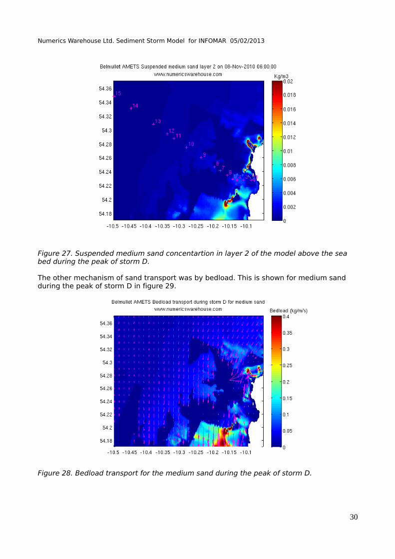
During the storm D, the amount of medium sand in suspension in layer 2 of the model, which corresponds to about 2 m above the seabed in 50 m depth is shown in figure 27. The amount of this finer sand suspended in the water column was quite low, except in shallow water. Above the the rocky areas there was almost no suspended sand, which shows that the sand, which has a fairly high settling velocity was not transported far.

29


Figure 27. Suspended medium sand concentartion in layer 2 of the model above the sea bed during the peak of storm D.

The other mechanism of sand transport was by bedload. This is shown for medium sand during the peak of storm D in figure 29.

Figure 28. Bedload transport for the medium sand during the peak of storm D.

30


Whereas the waves resuspend the sediment, the bedload direction is determined by the benthic tidal currents. The figure shows sand being carried onto the rocky area from adjacent sandy areas during the storm. The spatial proportion of the medium sand compared to coarse sand both before and during the storm D is shown in figure 29.

Figure 29. Proportion of medium sand to coarse sand in the upper exposed layer before the storm D (top) and at the peak of storm D (bottom).

The difference between the pre-storm period and the storm itself are not large. We can see some deposition of medium sand at the north of the rocky area has taken place and some other changes around the periphery of the rocky area. Similar changes were apparent after storm E.

31


Finally we can see the ripple height that was found at the peak of storm D in figure 30.

Figure 30. Ripple height at the peak of storm D.

The ripples were enhance in areas which had a higher median grain diameter, i.e. a mixture with more coarse sand in the upper exposed layer.

32


13. Conclusions from this Study

(1) The coupled wave-hydrodynamic-sediment transport modelling system has been successfully established and made to work at high resolution in an area of potential importance for ocean energy. This was one of the main aims of the project.

(2) The coupled model was run for a 3.5 month period correponding with some significant storms in the area to assess their effect on the sea bed sediments.

(3) By using INFOMAR supplied bathymetric data to describe the shape of the sea bed in the model and acoustic backscatter data to derive the main surface sediment properties, it has been possible to run a simulation which did not alter in a very substantial way the sediment properties. In other words the simulation was stable and can be considered as being realistic, with a requirement to only spin up the coupled model for a few days to achieve a quasi steady state. This will make the methodology developed here useful in other geographical areas to ocean energy customers such as offshore wind developers, wave energy developers or tidal turbine developers. The methodology of combining acoustic backscatter derived sediment properties with numerical coupled models is practical and should be useful for site selection, to design engineers or those planning operations and maintenance work in the ocean energy field.

(4) Five significant storms have been simulated using the coupled modelling system. It was shown that only a coupled wave-hydrodynamic-sediment model such as the COAWST system could adequately address all the dynamic features required to show the effect of these storms on the seabed sediments.

(5) It was shown that the rocky areas identified by the acoustic refection data supplied by INFOMAR corresponded well with areas of high bed shear stress due to a combination of tides, waves and other currents. It is believed that the waves were primarily responsible for suspending the sediment and that the bedload transport was the main mechanism for the sediment transport in this area.

(6) In this highly dynamic exposed environment around Belmullet, the storms did not have a big effect on the sediments, which were comprised anyway of coarse and medium sand, with significant areas of exposed rocky seabed. This will be a relief to any ocean energy enterprises planning on siting wave energy converters in AMETS. This conclusion should be checked using acoustic techniques. If this coupled modelling methodology were to be applied to the sandy areas of the Irish sea for example where future offshore wind turbines might be situated, it is expected that much more dramatic sediment changes might occur during storms.

(7) The use of coupled wave-hydrodynamic and sediment modelling has been shown to be useful in extending the knowledge of surface sediment properties from known acoustic and sampling measurements to adjacent areas where there was no data. This is a tentative conclusion and requires more work to understand properly.

(8) The modelling system can be used to extend the INFOMAR type multibeam derived snapshots into another dimension of time. This extends the usefulness of the INFOMAR datasets.

(9) It is expected that the type modelling conducted here would be useful in other fields of research such as in the classification of benthic habitats, since it would be possible to more fully describe the instantaneous peak velocities that animals would be subjected to and

33


the variability of the sediment thickness and classification.

14. Acknowledgements

The author is most grateful to Eimear O'Keeffe of INFOMAR for supplying the acoustic sediment data used in this study, to Deirdre O'Driscoll of the Marine Institute or supplying the INFOMAR bathymetry data and to Kieran Lyons of the Marine Institute for supplying the boundary data from their NE Atlantic model simulation.

I am also grateful to and acknowledge here the support of an INFOMAR innovation award to conduct this study.

34

Documents

A Study of the Effect on Seabed Sediments at Ocean Energy ... · Numerics Warehouse Ltd. Sediment Storm Model for INFOMAR 05/02/2013 A Study of the Effect on Seabed Sediments at Ocean