Embed Size (px)
Citation preview

Louisiana State UniversityLSU Digital Commons
LSU Historical Dissertations and Theses Graduate School
2001
A Study of the Applicability of IntrusionTechnology for Evaluating Resilient Modulus ofSubgrade Soil.Ananda H. m. p. j HerathLouisiana State University and Agricultural & Mechanical College
Follow this and additional works at: https://digitalcommons.lsu.edu/gradschool_disstheses
This Dissertation is brought to you for free and open access by the Graduate School at LSU Digital Commons. It has been accepted for inclusion inLSU Historical Dissertations and Theses by an authorized administrator of LSU Digital Commons. For more information, please [email protected].
Recommended CitationHerath, Ananda H. m. p. j, "A Study of the Applicability of Intrusion Technology for Evaluating Resilient Modulus of Subgrade Soil."(2001). LSU Historical Dissertations and Theses. 343.https://digitalcommons.lsu.edu/gradschool_disstheses/343

INFORMATION TO USERS
This manuscript has been reproduced from the microfilm master. UMI films the text directly from the original or copy submitted. Thus, some thesis and dissertation copies are in typewriter face, while others may be from any type of computer printer.
The quality of this reproduction is dependent upon the quality of the copy submitted. Broken or indistinct print, colored or poor quality illustrations and photographs, print bleedthrough, substandard margins, and improper alignment can adversely afFect reproduction.
In the unlikely event that the author did not send UMI a complete manuscript and there are missing pages, these will be noted. Also, if unauthorized copyright material had to be removed, a note will indicate the deletion.
Oversize materials (e.g., maps, drawings, charts) are reproduced by sectioning the original, beginning at the upper left-hand comer and continuing from left to right in equal sections with small overlaps.
Photographs included in the original manuscript have been reproduced xerographically in this copy. Higher quality 6” x 9” black and white photographic prints are available for any photographs or illustrations appearing in this copy for an additional charge. Contact UMI directly to order.
ProQuest Information and Learning 300 North Zeeb Road. Ann Arbor, Ml 48106-1346 USA
800-521-0600
Reproduced with permission of the copyright owner. Further reproduction prohibited without permission.

Reproduced with permission of the copyright owner. Further reproduction prohibited without permission.
A STUDY OF THE APPLICABILITY OF INTRUSION TECHNOLOGY FOR EVALUATING RESILIENT
MODULUS OF SUBGRADE SOIL
A Dissertation
Submitted to the Graduate Faculty of the Louisiana State University and
Agricultural and Mechanical College in partial fulfillment of the
requirements for the degree of Doctor of Philosophy
in
The Department of Civil and Environmental Engineering
byAnanda H M JJ . Herath
B.S., University of Peradeniya, Sri Lanka, 1983 M.S., University of Tokyo, Japan, 1988
August 2001
Reproduced with permission of the copyright owner. Further reproduction prohibited without permission.

UMI Number: 3021432
UMI"UMI Microform 3021432
Copyright 2001 by Bell & Howell Information and Learning Company. All rights reserved. This microform edition is protected against
unauthorized copying under Title 17, United States Code.
Bell & Howell Information and Learning Company 300 North Zeeb Road
P.O. Box 1346 Ann Arbor, Mi 48106-1346
Reproduced with permission of the copyright owner. Further reproduction prohibited without permission.

DEDICATION
This work is dedicated to my parents, late Mr. R.B.Herath, father, and Mrs.
T.M.Herath, mother, for their invaluable sacrifice and constant inspiration throughout my
education. This is also dedicated to my wife, Suba Herath, and my children.
ii
Reproduced with permission of the copyright owner. Further reproduction prohibited without permission.

ACKNOWLEDGMENTS
My deepest appreciation and sincere thanks to Dr. Louay N. Mohammad,
my advisor, for his guidance and encouragement throughout the study. Without his support
and constant inspiration, this study would not have been successful.
I wish to extend my appreciation to Dr. John B. Metcalf, my co-advisor, for his
support and valuable direction in this study.
My sincere thanks to Dr. Mehmet T. Tumay, my minor professor, for providing the
Continuous Intrusion Miniature Cone Penetration Test system and Research Vehicle for
Geotechnical In-situ Testing and Support, which were developed by him. Without his
dedication to the cone penetration test area during the last two decades, I would not have
been able to do this research.
I would also express my appreciation to Dr. Hani H. Titi for his time and valuable
advice throughout this research.
I am also very grateful to the other distinguished members of my committee,
Dr. Lynn R. LaMotte, and Dr. Jim Chambers for their support and valuable suggestions in
this study.
Special thanks are also offered to Mr. William T. Tierney for his efforts in conducting
the cone penetration tests. I wish to acknowledge Amar Raghavendra for his help and
encouragement with the laboratory tests. I would like to thank to Mark Morvant, Paul Brady,
Melba Bounds, Kenneth Johnson, Jason Flory, Michael Cooper, David Wedlake, Robert
Glen Graves, Willie Gueho, Greg Tullier, Baoshan Huang, and Dr. Khalid Farrag for their
help with laboratory testing.
iii
Reproduced with permission of the copyright owner. Further reproduction prohibited without permission.

TABLE OF CONTENTS
DEDICATION................................................................................................................. ii
ACKNOWLEDGMENTS................................................................................................ iii
LIST OF TABLES......................................................................................................... vii
LIST OF FIGURES........................................................................................................ viii
LIST OF ABBREVIATIONS.........................................................................................xiv
ABSTRACT.....................................................................................................................xvi
CHAPTER 1 INTRODUCTION ...................................................................................... 11.1 Problem Statement............................................................................................ I
CHAPTER 2 BACKGROUND ........................................................................................72.1 Introduction......................................................................................................72.2 Resilient M odulus............................................................................................72.3 Cone Penetration Test .................................................................................. 112.4 Limitation........................................................................................................ 132.5 Objectives ...................................................................................................... 142.6 Scope of the Study.......................................................................................... 15
CHAPTER 3 LABORATORY AND FIELD TESTING................................................ 153.1 Introduction.................................................................................................... 153.2 Laboratory Testing Program .......................................................................... 15
3.2.1 Equipment for the Resilient Modulus Testing ................................ 153.2.2 Loading System .............................................................................. 153.2.3 Digital C ontroller............................................................................ 153.2.4 Load Unit Control Panel..................................................................203.2.5 Triaxial Cell ....................................................................................203.2.6 Pressure Control Panel ....................................................................203.2.7 LVDTs and Load C ell......................................................................203.2.8 Data Acquisition and Equipment Control........................................2232.9 Laboratory Resilient Modulus Testing Procedure ..........................22
3.3 Field Testing Program ....................................................................................223.3.1 Description of the Test S ites............................................................233.3.2 Research Vehicle for Geotechnical In-situ
Testing and Support (REVIGITS)................................................233.3.3 Continuous Intrusion Miniature
Cone Penetration Test (CIMCPT or M CPT)................................253.3.4 Procedure ........................................................................................2533.5 Laboratory Soil Property T esting................................................. 28
iv
Reproduced with permission of the copyright owner. Further reproduction prohibited without permission.

3.4 Laboratory Cone Penetration Testing ........................................................... 283.4.1 Introduction..................................................................................... 283.4.2 O bjectives....................................................................................... 323.4.3 Methodology................................................................................... 323.4.4 Equipment for the Laboratory Cone T es t........................................323.4.5 Data Acquisition System................................................................. 343.4.6 Testing program ............................................................................. 34
3.4.6.1 Soil Compaction ............................................................. 343.4.6.2 Cone Testing ................................................................... 373.4.6.3 Soil Testing ..................................................................... 373.4.6.4 Resilient Modulus Testing................................................40
CHAPTER 4 ANALYSIS OF RESULTS ..................................................................... 414.1 Soil Characterization..................................................................................... 41
4.1.1 Pavement Research F acility ........................................................... 414.1.2 State Route LA-42 (Highland Road) at 1-10 ..................................444.1.3 State Route LA-15 ......................................................................... 444.1.4 State Route LA-89/ New Iberia ..................................................... 444.1.5 Siegen Lane/ Baton R ouge............................................................. 444.1.6 State Route LA-28/ Simpson ......................................................... 454.1.7 State Route LA-1/ Larose............................................................... 45
4.2 Cone Test Results ......................................................................................... 454.3 Resilient Modulus Test R esults..................................................................... 704.4 Model Development....................................................................................... 81
4.4.1 Proposed Model for Fine-grained Soils (in-situ) ............................864.4.2 Proposed Model for Coarse-grained Soils (in-situ) ........................874.4.3 Analysis for Traffic Loadings..........................................................92
4.4.3.1 Traffic Stress Model for Fine-grained Soil ......................924.4.3.2 Traffic Stress Model for Coarse-grained Soil ..................94
4.5 Analysis o f the Laboratory Cone Penetration Test ........................................964.5.1 Effects o f Compaction ................................................................... 964.5.2 Boundary Effects ........................................................................... 964.5.3 Laboratory Cone Penetration Test Results .................................. 1034.5.4 Resilient Modulus ....................................................................... 1174.5.5 Effect of Moisture Content and Unit W eight................................ 1264.5.6 Summary of the Laboratory Cone T esting.................................... 1284.5.7 Traffic Stress A nalysis..................................................................1334.5.8 Preliminary Design C harts............................................................133
4.5.8.1 A Chart for Estimating Effective Subgrade Soil Resilient Modulus Using the Serviceability C riteria.....................149
4.5.8.2 An Example for Using the Proposed C h a rts ..................1524.6 Sensitivity o f the AASHTO Flexible Pavement Design Equation ..............153
CHAPTER 5 FIELD APPLICATION OF THE PROPOSED MODELS......................157
v
Reproduced with permission of the copyright owner. Further reproduction prohibited without permission.

CHAPTER 6 SUMMARY AND CONCLUSIONS......................................................1676.1 Future Recommendations ......................................................................... 170
REFERENCES ............................................................................................................. 171
APPENDIX A RESILIENT MODULUS TEST RESULTS ......................................176
APPENDIX B PROCEDURE FOR MODEL DEVELOPMENT..............................181
VITA ............................................................................................................................. 186
vi
Reproduced with permission of the copyright owner. Further reproduction prohibited without permission.

LIST OF TABLES
Table 3.1 Laboratory testing program for soil testing .............................................. 17
Table 3.2 Field testing program ...............................................................................18
Table 3.3 The moisture-unit weight combinations used in the tests.........................31
Table 3.4 Laboratory cone testing program .............................................................39
Table 4.1 Properties of fine-grained soils used in the investigation.........................42
Table 4.2 Properties of coarse-grained soils used in the investigation.....................43
Table 4.3 Summary of the field cone penetration and laboratory tests on soils . . . 83
Table 4.4 Summary of the stress analysis on the investigated soils .......................84
Table 4.5 Elastic properties of the investigated s o ils .............................................. 85
Table 4.6 Summary of the field and laboratory tests on the LA-28 sandand LA-89 lime treated recycled soil-cement ..............................90
Table 4.7 Summary of the stress analysis on the LA-28 sand and LA-89lime treated recycled soil-cement ............................................... 90
Table 4.8 Properties of the soils used in the laboratory cone penetration t e s t 99
Table 4.9 Summary of the laboratory cone test results .........................................136
Table 4.10 Stress analysis for the laboratory cone te s ts ...........................................137
Table 4.11 Elastic properties of soils ...................................................................... 138
Table 4.12 Cone penetration and soil test data for silty clay ...................................152
Table 5.1 Summary of the test results .................................................................. 166
Table 52 Summary of the stress analysis ...........................................................166
Reproduced with permission of the copyright owner. Further reproduction prohibited without permission.

LIST OF FIGURES
Figure 1.1 Typical pavement sections...........................................................................2
Figure 1.2 The definition of the resilient modulus .......................................................4
Figure 2.1 Load pulse used in the AASHTO T- 294 testing procedure ....................... 9
Figure 2.2 A typical friction cone penetrometer......................................................... 12
Figure 3.1 Locations o f the field testing s ite s ............................................................. 16
Figure 3.2 The MTS system ....................................................................................... 19
Figure 3.3 Closed loop control system in the M TS.....................................................21
Figure 3.4 The REVIGITS system ............................................................................ 24
Figure 3.5 The CIMCPT System................................................................................ 26
Figure 3.6 The 15 cm2 cone, 2 cm2 miniature cone, and a ball point pen ................ 27
Figure 3.7 A typical layout for the field cone penetration test at a s i te ..................... 29
Figure 3.8 The laboratory cone test setup ................................................................. 33
Figure 3.9 The data acquisition system for the miniature cone penetration ............. 35
Figure 3.10 A typical layout for the laboratory cone test for compacted soils .......... 38
Figure 4.1 Field test layout for the PRF-silty c la y .................................................... 46
Figure 4.2 Cone penetration test results of the PRF-silty clay (set # 1 ) ..................... 47
Figure 4.3 Coefficient o f variation for the cone test of the PRF-silty clay ...............49
Figure 4.4 Field test layout for the PRF-heavy clay ................................................... 50
Figure 4.5 Cone penetration test results of the PRF-heavy clay (set # 1 )................... 52
Figure 4.6 Coefficient o f variation for the cone test of the PRF-heavy c la y 53
Figure 4.7 Field test layout for the LA-42/1-10 s ite .................................................. 54
Figure 4.8 Cone penetration test results of the LA-42/1-10 site (set # 1 ) ...................55
viii
Reproduced with permission of the copyright owner. Further reproduction prohibited without permission.

Figure 4.9 Coefficient o f variation for the cone test of the LA-42/1-10 site ............56
Figure 4.10 Field test layout for the LA-15 s ite ........................................................... 58
Figure 4.11 Cone penetration test results of the LA-15 site (set # 1 ) ...........................59
Figure 4.12 Coefficient of variation for the cone test of the LA-15 site .....................60
Figure 4.13 Field test layout for the LA-89 s ite ...........................................................61
Figure 4.14 Cone penetration test results o f the LA-89 site (set # 1 ) ...........................62
Figure 4.15 Coefficient o f variation for the L A -89.....................................................63
Figure 4.16 Field test layout for the Siegen Lane s i te .................................................64
Figure 4.17 Cone penetration test results of the Siegen Lane site (set #1) ................ 65
Figure 4.18 Coefficient of variation for the Siegen Lane ...........................................66
Figure 4.19 Cone penetration test results of the LA-28 site (set # 1 ) .......................... 68
Figure 4.20 Coefficient of variation for the LA-28 (Set#l) .......................................69
Figure 4.21 Resilient modulus of the PRF-silty clay at borehole 1 ........................... 71
Figure 4.22 Resilient modulus of the PRF-heavy clay at borehole 1 ......................... 73
Figure 4.23 Resilient modulus of the LA42/I-10 clay at borehole 2 .......................... 75
Figure 4.24 Resilient modulus of the LA-15 clay at borehole 1 ................................ 76
Figure 4.25 Resilient modulus o f the LA-89 clay at borehole 2 ................................ 77
Figure 4.26 Resilient modulus o f the Siegen Lane clay .............................................. 79
Figure 4.27 Resilient modulus o f LA-28 sand .......................................................... 80
Figure 4.28 Interpolation procedure for resilient modulus.......................................... 82
Figure 4.29 Prediction of in-situ resilient modulus for fine-grained so il.................... 88
Figure 4.30 Prediction of in-situ resilient modulus for coarse-grained so il................ 91
Figure 4.31 A typical pavement structure for traffic stress analysis .......................... 93
ix
Reproduced with permission of the copyright owner. Further reproduction prohibited without permission.

Figure 4.32 Prediction of resilient modulus of fine-grained soil fromthe traffic stress m odel................................................................. 95
Figure 4.33 Predicted and measured resilient modulus forcoarse-grained soil (traffic) ......................................................... 97
Figure 4.34 Moisture-unit weight relationship of the PRF-silty clay......................... 100
Figure 4.35 Moisture-unit weight relationship of the PRF-heavy c la y ..................... 100
Figure 4.36 Moisture-unit weight relationship of silt ...............................................101
Figure 4.37 Moisture-unit weight relationship of sand .............................................101
Figure 4.38 Effect of the layered compaction of so ils ...............................................102
Figure 4.39 Laboratory cone penetration of silty clay at dry s id e .............................104
Figure 4.40 Coefficient of variation of laboratory cone penetration ofsilty clay at dry s id e ................................................................... 106
Figure 4.41 Laboratory cone penetration of silty clay at the optimum 107
Figure 4.42 Coefficient of variation of laboratory cone penetration o fsilty clay at optim um ................................................................. 108
Figure 4.43 Laboratory cone penetration of silty clay at wet side .........................109
Figure 4.44 Coefficient of variation of laboratory cone penetration ofsilty clay at wet side ................................................................. 110
Figure 4.45 Laboratory cone penetration of heavy clay at dry side .........................112
Figure 4.46 Coefficient o f variation of laboratory cone penetration ofheavy clay at dry side ............................................................... 113
Figure 4.47 Laboratory cone penetration o f heavy clay at optimum ........................ 114
Figure 4.48 Laboratory cone penetration of heavy clay at wet s id e .......................... 115
Figure 4.49 Laboratory cone penetration of s i l t ........................................................116
Figure 4.50 Laboratory cone penetration o f sa n d ......................................................118
Figure 4.51 Resilient modulus o f silty clay at dry s id e ............................................ 119
x
Reproduced with permission of the copyright owner. Further reproduction prohibited without permission.

Figure 4.52 Resilient modulus o f silty clay at optimum ............................................120
Figure 4.53 Resilient modulus of silty clay at wet s id e ............................................. 121
Figure 4.54 Resilient modulus of heavy clay at dry side ......................................... 122
Figure 4.55 Resilient modulus of heavy clay at optim um ......................................... 123
Figure 4.56 Resilient modulus of heavy clay at wet side........................................... 124
Figure 4.57 Resilient modulus of silt at dry s id e ....................................................... 125
Figure 4.58 Resilient modulus of sand at dry side ..................................................127
Figure 4.59 Variation in the resilient modulus with moisture contentof fine-grained soil ....................................................................129
Figure 4.60 Variation in the resilient modulus with moisture contentof coarse-grained so il................................................................. 130
Figure 4.61 Variation o f the moisture content, unit weight, and resilientmodulus for fine-grained so il......................................................131
Figure 4.62 Variation o f the moisture content, unit weight, and resilientmodulus for coarse-grained s o i l ................................................ 131
Figure 4.63 Variation o f the moisture content, unit weight, and tipresistance for fine-grained soil .................................................. 132
Figure 4.64 Variation of the moisture content, unit weight, and tipresistance for coarse-grained s o i l .............................................. 132
Figure 4.65 In-situ resilient modulus from the laboratory cone test forfine-grained soil ........................................................................134
Figure 4.66 In-situ resilient modulus from the laboratory cone test forcoarse-grained s o il......................................................................135
Figure 4.67 Prediction of resilient modulus from the traffic stress model forfine-grained soil ........................................................................139
Figure 4.68 Prediction of resilient modulus from the traffic stress model forcoarse-grained soil ....................................................................140
Figure 4.69 A chart for estim ating in-situ resilient modulus o f silty c la y ................141
xi
Reproduced with permission of the copyright owner. Further reproduction prohibited without permission.

Figure 4.70 A chart for estimating in-situ resilient modulus of heavy clay fromcone penetration ...................................................................... 142
Figure 4.71 A chart for estimating in-situ resilient modulus of silt fromcone penetration ...................................................................... 143
Figure 4.72 A chart for estimating in-situ resilient modulus of sand fromcone penetration ...................................................................... 144
Figure 4.73 A chart for estimating resilient modulus of heavy clay fromcone penetration under traffic stress .........................................145
Figure 4.74 A chart for estimating resilient modulus of silty clay fromcone penetration under traffic stress .........................................146
Figure 4.75 A chart for estimating resilient modulus of silt fromcone penetration under traffic stress .........................................147
Figure 4.76 A chart for estimating resilient modulus of sand fromcone penetration under traffic stress .........................................148
Figure 4.77 A chart for estimating effective roadbed soil resilientmodulus using the serviceability criteria .................................151
Figure 4.78 Estimation of the effective resilient modulus fromcone test parameters ................................................................ 154
Figure 4.79 A typical pavement section ..................................................................155
Figure 4.80 Variation in the overlay thickness with the resilient m odulus.............. 156
Figure 5.1 Cone penetration test results of the LA-482 ........................................ 158
Figure 5.2 Cone penetration test results o f the LA-51 3 .......................................... 159
Figure 5.3 Cone penetration test results of theHenderson levee road .............................................................. 160
Figure 5.4 Resilient modulus test results of the LA-482 ........................................ 161
Figure 5.5 Resilient modulus test results of the LA-51 3 ........................................162
Figure 5.6 Resilient modulus test results of theHenderson levee road................................................................ 163
xii
Reproduced with permission of the copyright owner. Further reproduction prohibited without permission.
Figure 5.7 Prediction o f the resilient modulus underin-situ condition......................................................................... 164
Figure 5.8 Prediction of resilient modulus undertraffic loading ............................................................................165
Reproduced with permission of the copyright owner. Further reproduction prohibited without permission.

LIST OF ABBREVIATIONS
AASHTO American Association of State Highway and Transportation OfficialsALF Accelerated Load FacilityASTM American Society for Testing and MaterialsBH Boreholec Cohesion interceptCBR California Bearing RatioCICU Isotropically Consolidated Undrained Triaxial Compression TestCOV Coefficient of VariationCPT Cone Penetration TestCIMCPT Continous Intrusion Miniature Cone Penetrometer TestE Modulus of Elasticity (Young's modulus)ESAL Equivalent Single Axial LoadingEMCRF Engineering Materials Characterization Research FacilityFHWA Federal Highway AdministrationFWD Falling Weight Deflectometerf, Sleeve frictionG Shear modulusG, Specific gravity
Coefficient of lateral earth pressure at restLA DOTD Louisiana Department o f Transportation and DevelopmentLCD Liquid Crystal DisplayLL Liquid LimitLTRC Louisiana Transportation Research CenterLVDT Linear Variable Differential TransducerMTS Material Testing SystemMr Resilient modulusMCPT Miniature Cone Penetrometer TestNA Not availableNDT Nondestructive TestNP Non plasticPCPT Piezocone penetration testPI Plasticity IndexPL Plasticity LimitPRF Pavement Research Facilityqc Cone tip resistanceR ReliabilityR2 Coefficient o f multiple determinationREVEGITS Research Vehicle for Geotechnical In-situ Testing and SupportRMSE Root Mean Squared ErrorRr Friction ratioSAS Statistical Analysis SystemSHRP Strategic Highway Research ProgramSN Structural number
Reproduced with permission of the copyright owner. Further reproduction prohibited without permission.

S. Combined standard error of the traffic prediction and performance prediction
ssv Soil Support ValueSTD Standard deviationSu Undrained shear strengthTRB Transportation Research Boarduses Unified Soil Classification SystemUU Unconsolidated Undrained Triaxial Compression Testur Relative damagew water contentWop, Optimum water contentw„ Predicted number of 18-kip equivalent single axle loadZR Standard normal deviationYd Dry unit weightYdmax Maximum dry unit weightYw Unit weight of waterS r Axial strainO Poisson’s ratio
Major principal stress<*3 Minor principal stress<*c Confining stressCTd Deviator stress<*h Horizontal stressCTy Vertical stress♦ Angle of internal frictionAPSI Difference between the initial design serviceability index and the design
terminal serviceability index.
XV
Reproduced with permission of the copyright owner. Further reproduction prohibited without permission.
ABSTRACT
The cone penetration test may be applied for estimation of the resilient modulus
o f subgrade soil. The main objectives of this study were to assess the applicability of the
intrusion technology in evaluating the resilient characteristics of subgrade soil, develop
models among the cone penetration test parameters, resilient modulus, soil properties,
and stresses of subgrade soil, and to validate these models.
Field cone penetration and laboratory tests were performed on different soil types.
Disturbed and undisturbed soil samples were obtained close to the cone penetration test
locations. Laboratory tests were also performed to obtain the resilient modulus, strength
parameters, compaction characteristics, and physical properties of subgrade soil. The
results of the laboratory soil properties, resilient modulus, and eight field cone
penetration tests are presented.
The models, among the cone penetration parameters, resilient modulus, moisture
content, dry unit weight, and stress levels, were developed. Both in-situ stresses and
induced traffic stresses were considered. Four models were developed for fine-grained
and coarse-grained soil with in-situ and traffic stress conditions. These models were
calibrated using the field test results of two soil types and used to predict the resilient
modulus of different soil types.
The cone penetration, resilient modulus, and soil property tests were also
performed on the laboratory compacted soil samples to investigate the effects of the
variation in the moisture content and unit weight on the resilient modulus as well as to
validate the proposed models. Special test equipment and a miniature cone with a
straight push rod were developed for the laboratory cone testing. Four soil types and
xvi
Reproduced with permission of the copyright owner. Further reproduction prohibited without permission.

three levels of moisture contents, such as dry side, optimum, and wet side, were selected
for this testing. The results of the laboratory soil property, resilient modulus, and twelve
laboratory cone penetration tests are presented. Simplified design charts, based on the
cone penetration parameters and resilient modulus, were also developed. The proposed
models were implemented in the selected road rehabilitation projects.
xvii
Reproduced with permission of the copyright owner. Further reproduction prohibited without permission.

CHAPTER 1
INTRODUCTION
This dissertation presents the research effort and conclusions o f the assessment of
the applicability of the intrusion technology for evaluating resilient modulus of subgrade
soil. Chapter 1 includes the introduction and the problem statement. Chapter 2 presents
background, limitation, objectives, and scope of the study. Chapter 3 describes the
laboratory and field testing program that includes a brief description of the field and
laboratory testing equipment and testing procedures. Chapter 3 also presents the
laboratory cone penetration testing (controlled testing) program. Chapter 4 presents the
analysis of results. Chapter S includes the field application of the proposed correlations
in the selected rehabilitation projects. Chapter 6 presents the summary and conclusions.
1.1 Problem Statement
Flexible and rigid pavements are the major pavement types used in roadways.
Figure 1.1 depicts the typical structural layers of each pavement type. Figure 1.1 (a)
shows a rigid pavement that consists of a Portland cement concrete slab, base or subbase,
and subgrade. The pavement slab consists of Portland cement concrete, reinforcing steel,
load transfer devices, joints, and sealing materials.
Figure 1.1 (b) presents a flexible pavement that consists o f a surface course
(asphalt concrete wearing and binder course layers), base, subbase, and subgrade. The
base is located immediately below the surface course. It consists o f crushed stone,
crushed gravel and sand, or crushed slag. Subbase is located between the subgrade and
base. It consists of a compacted layer o f granular materials or a layer o f treated soil.
Subgrade is a compacted in-situ soil or borrow material.
1
Reproduced with permission of the copyright owner. Further reproduction prohibited without permission.

Portland cement concrete slab Surface wearing course Binder course
BaseSub base
Sub base
Subgrade Subgrade
(a) A rigid pavement (b) A flexible pavement
Figure 1.1 Typical pavement sections
Static properties, such as California Bearing Ratio (CBR) and soil support value
(SSV), used for flexible pavement design and subgrade soil characterization, do not take
into account the dynamic response of the moving vehicles. In order to incorporate this
dynamic behavior, the resilient modulus was introduced in the mechanistic design of
pavements by the American Association of State Highway and Transportation Officials
(AASHTO) guide for design of pavement structures (1986,1993, and the proposed 2002).
After its introduction, the resilient modulus gained popularity in the pavement design.
The resilient modulus is the definitive material property used to characterize subgrade
soil in pavement structures. The subgrade soil charaterization, based on the resilient
modulus, is a realistic way to analyze the moving vehicle loads on a pavement. The
resilient modulus represents the dynamic stiffness of pavement materials under repeated
loading of the moving vehicles.
In flexible pavement design, the resilient modulus is a direct input parameter. The
AASHTO design equation, as presented in Section 4.6, Chapter 4, includes the subgrade
resilient modulus along with other parameters, such as traffic loading, change in Present
2
Reproduced with permission of the copyright owner. Further reproduction prohibited without permission.
Serviceability Index (PSI), reliability, and standard deviation. This design equation
estimates the structural number (SN) and then it estimates the pavement thickness using
the structural coefficients of each layer. In rigid pavement design, the subgrade resilient
modulus is to be converted to a modulus of subgrade reaction (k-value).
The resilient modulus denotes a basic constitutive relationship between stress and
deformation of materials. The resilient modulus (Mr) is the ratio o f the deviator axial
stress (cTd) to the recoverable (resilient) axial strain (e,). Figure 1.2 illustrates the
definition of the resilient modulus.
The resilient modulus can be estimated from the empirical correlations, in-situ
nondestructive testing, and laboratory testing on soil samples. Several empirical
correlations have been reported (Uzan 1985; AASHTO, 1986; Pezo et al., 1994; Allen,
1996; Mohammad et al., 1998, 1999, and 2000) which can be used to estimate resilient
modulus from soil support value, CBR, stress levels, and soil properties. Laboratory test
methods and in-situ nondestructive test methods (NDT) are also used to evaluate the
resilient modulus. The laboratory tests require sophisticated equipment and skilled
technicians. Also, laboratory test methods are considered laborious, time consuming, and
expensive. On the other hand, the backcalculated resilient modulus from in-situ
nondestructive test results may have low repeatability. The resilient modulus values from
the NDT were greater than those from the laboratory tests (AASHTO guide for design of
pavement structures, 1993) and they must be adjusted before use in the design o f flexible
3
Reproduced with permission of the copyright owner. Further reproduction prohibited without permission.

Resilient modulus, Mr = ------
eaa.■a0
enGOsn
><uQ
Legend
<yd = Deviator stress Ep, = Plastic strain
e, = Resilient strain
&r = Total axial strain
Strain, s (%)
Figure 1.2 The definition of the resilient modulus
4
Reproduced with permission of the copyright owner. Further reproduction prohibited without permission.
pavements. If not, it will result in an under designed pavement structural layer. The
design resilient modulus value has an effect on the design structural number and hence
on the overlay thickness in the pavement. The higher the resilient modulus value, the
thinner the overlay thickness in the pavement.
The above mentioned limitations of the laboratory test and NDT methods imply a
necessity of an alternative in-situ test method to evaluate the resilient properties of
subgrade soil. Because of its rapidity and simplicity, the cone penetration testing (CPT)
has become a popular in-situ test method. Also, the CPT results are repeatable and
reliable (Campanella and Robertson, 1981; Tumay, 1981). The CPT data has
successfully been used to evaluate soil classification, soil stratigraphy, shear strength, and
deformation properties of soil, such as Young’s modulus (E) and shear modulus (G)
(Schmertmann, 1978; Campanella and Robertson, 1981; Robertson and Campanella,
1983). These interpretation methods are based on empirical correlations, theoretical and
analytical approaches. It is expected that the CPT method may also be applied for
evaluating the resilient modulus of subgrade soil.
An experimental program was performed to study the application of the CPT in
evaluating the resilient modulus of subgrade soil. To accomplish this objective, different
subgrade soil sites in Louisiana were selected for the field cone penetration and
laboratory testing. The soil types included fine-grained and coarse-grained soil. The
field cone penetration tests included 15 cm2 friction cone penetrometer tests and 2 cm2
continuous intrusion m iniature cone penetration tests. Disturbed and undisturbed soil
samples were obtained close to the cone penetration test locations. The laboratory tests
were also performed to obtain the resilient modulus, strength parameters, compaction
5
Reproduced with permission of the copyright owner. Further reproduction prohibited without permission.

characteristics, and physical properties o f subgrade soil. The implementation of the
miniature cone penetration test was verified. Statistical models were developed to
correlate the resilient modulus, the cone penetration test parameters, stress levels (in-situ
or traffic), moisture content, and unit weight. The resilient moduli were evaluated for
both the in-situ and traffic loading conditions. These models were developed, based on
the results o f two field soil types, and used to evaluate the resilient modulus of other
soils. The proposed models were validated by the test results of the rest of the field tests.
The measured and predicted resilient modulus values were not significantly different.
The laboratory cone penetration tests were also performed on the compacted soil samples
of four soil types at three different moisture content levels, such as dry side, optimum,
and wet side, to study the effects o f variation in the moisture content on the resilient
modulus, establish preliminary design charts, and validate the models. Insufficient data
was available to verify the preliminary design charts. The use o f the preliminary design
charts or proposed models, to compute an effective subgrade soil resilient modulus, was
illustrated.
The proposed models were successfully implemented in the road rehabilitation
projects, such as LA-482, LA-513, and Henderson levee road. A quick and effective
assessment of pavement subgrade soil resilient properties with the cone penetration test
will provide a cost-effective input to pavement design.
6
Reproduced with permission of the copyright owner. Further reproduction prohibited without permission.
CHAPTER 2
BACKGROUND
2.1 Introduction
This chapter presents the literature review of the resilient modulus and cone
penetration tests, limitations, objectives, and scope of the study.
2.2 Resilient Modulus
The resilient modulus is estimated from the backcalculation of the NDT deflection
results, laboratory triaxial testing on soil samples, and correlations with soil properties,
CBR, and soil support values. The Dynaflect, Road Rater, and Falling Weight
Deflectometer (FWD) are the devices used for NDT test methods. These NDT methods
measure the deflection of the pavement under a loading. These deflections are used in
backcalculation subroutines to evaluate the resilient modulus. Backcalculated modulus
depends on many factors, such as loading condition and stiffness in layers (Sebaaly et al.,
1992; Lee et al., 1994).
There are many laboratory testing devices used for determ ining the resilient
modulus of subgrade soil. The devices used for laboratory testings are tri axial cell,
resonant column, simple shear device, torsional apparatus, hollow cylinder and true
tri axial cell. Because of its simplicity, repeatability and accuracy, the tri axial cell is the
most popular laboratory testing device. But these laboratory tests are laborious, time
consuming, and expensive.
In 1986, AASHTO recommended the testing procedure, T 274-82, to determine
the resilient modulus of subgrade soil. Inadequate conditioning steps and over stressing
the sample were reported in this test procedure (Mohammad et al., 1993; Nazarian, 1993).
7
Reproduced with permission of the copyright owner. Further reproduction prohibited without permission.

The major drawback of the T 274-82 was that the stresses were so high that the specimen
may be damaged in the preconditioning stage. The AASHTO T 274-82 test procedure
was modified and replaced by an interim AASHTO procedure T 292-911. Then in 1992,
AASHTO adopted the Strategic Highway Research Program (SHRP) Protocol 46
(AASHTO T 294-921). After including the previous developments in the test procedure
for determination of the resilient modulus o f subgrade soil, the current test procedure,
T 294-94, was introduced. This procedure requires a test system that includes a tri axial
cell, a closed loop electro-hydraulic repeated loading system, load and specimen response
control system, and measurement and recording system. Figure 2.1 shows the load pulse
used in this test method. In order to simulate traffic loadings, AASHTO T 294-94
recommends the haversine-shaped load pulse with a 0.1 second load followed by a 0.9
second rest period.
Resilient modulus is influenced by many factors. Many investigators (Rada et al.,
1981; Kamal et al., 1993; Mohammad et al., 1994) observed an increase in resilient
modulus of granular materials with increase in confining pressure. This is due to the fact
that increase in stiffness and decrease in dilational properties o f granular soil. The
resilient modulus of cohesive soil decreases as deviator stress increases (Fredlund et al.,
1977). The same observations were made by Mohammad et al., (1998 and 1999) for
cohesive soils. These observations confirm the stress and dilational property dependent
nature o f the resilient modulus o f subgrade soil. Many researchers have studied the effect
o f moisture content on resilient modulus of soil (Allen, 1989; McGee, 1989; Monismith,
1989; Mohammad et al., 1995; Drumm et al., 1997; Mohammad et al., 2000). They
reported that resilient modulus o f cohesive soil decreases as the moisture content
8
Reproduced with permission of the copyright owner. Further reproduction prohibited without permission.

I_oes‘>uQ
O.i 0.9
Time (s)
Figure 2.1 Load pulse used in the AASHTO T- 294 testing procedure
increases. The resilient modulus can be influenced by the seasonal variation of moisture
in soil, such as repeated freeze-thaw cycle. Several investigators (Nataatmadja et al.,
1989; Mohammad et al., 1994) reported that the resilient modulus can also be influenced
by dry unit weight, size of the specimen, stress pulse shape, duration, frequency and
sequence of stress levels, testing equipment, and specimen preparation as well as
conditioning methods.
When the load is repeated thousands of times, the nonlinear behavior o f subgrade
soil is reduced. After thousands of times application of the load, plastic deformation is
virtually completed. Then the soil sample response is virtually elastic and linear
9
Reproduced with permission of the copyright owner. Further reproduction prohibited without permission.

(AASHTO, 1992). Based on this, AASHTO T 294-94 recommends using one thousand
cycles of preconditioning load to the specimen. At each stress level during the testing,
T 294-94 test procedure requires 100 cycles of loadings to the specimen. Resilient
modulus is determined by taking the average of the last five cycles.
Several empirical correlations have been developed to predict the results o f the
resilient modulus test (Uzan 1985; AASHTO, 1986; Pezo et al., 1994; Allen, 1996;
Mohammad et al., 1998, 1999, and 2000). For granular materials, the relationship given
below may be used as recommended by the AASHTO.
This is known as the bulk stress model. The AASHTO recommended the deviator
stress model for cohesive soil. It is given by,
where,
M r - resilient modulus,
k , , k 2, &j,and k4 - material constants,
ou - deviator stress = oy - oy,
a ,—major principal stress, ay- intermediate principal stresses, and o> -minor principal
stress, and
0 - bulk stress =cr,+ oy-foy.
The bulk stress model is very simple. However, the disadvantages those are the
bulk stress model does not show individual effects of the deviator and confining stresses
(2.1)
K = ki<Jd k‘ (2.2)
10
Reproduced with permission of the copyright owner. Further reproduction prohibited without permission.

while the deviator stress model does not show the significance of the confining stress on
cohesive soil (Ullidtz, 1987; Nataatmadja et al., 1989).
Mohammad et al. (1999,2000) proposed an octahedral stress model to over come
some of the limitations discussed above. This model takes into account the effects of
shear and influence of the stress state. This model can be used for both fine-grained and
coarse-grained soils. The model considers the octahedral shear and normal stresses. The
octahedral model is given as follows,
where, M r is the resilient modulus, k , , k 2, and k} are material constants, crxt is the
octahedral normal stress, fxl is the octahedral shear stress, and is the atmospheric
pressure (0^=101.35 kPa). Many researchers correlated resilient modulus with strength
and physical properties of soil such as California Bearing Ratio, moisture content,
plasticity index, confining pressure and deviator stress (AASHTO, 1986; Allen, 1986;
Carmichael III et al., 1986; Mohammad et al., 1999; Puppala et al., 1999; Mohammad et
al., 2000). But these models have to be calibrated and validated for local conditions. This
requires a significant effort and experimental work. Therefore use of these models are
considered time consuming, laborious, and expensive.
2 3 Cone Penetration Test
The cone penetration test provides a rapid, continuous reading of tip resistance
(q j and sleeve friction (Q as the cone penetrates into the ground. As shown in
Figure 2.2, the CPT consists of a series of cylindrical push rods with a cone at the bottom.
(2.3)
11
Reproduced with permission of the copyright owner. Further reproduction prohibited without permission.

The penetration resistance is related to the strength of the soil. The tip resistance depends
on the size of the cone tip, rate of penetration, types of soil, density and moisture content
(Schmertmann, 1978). The standard cone has a projected tip area of 10 cm2 and an apex
angle of 60 degrees.
(X Ring O- Ring
Friction Sleeve Push RodCone Tip
Figure 2.2 A typical friction cone penetrometer
A typical friction sleeve, located immediately above the tip, has 150 cm2 surface
area for the 10 cm2 cones and 200 cm2 for the 15 cm2 cones. A 20 mm/ sec penetration
rate is normally used in the standard tests. The CPT and piezocone penetration tests
(with pore water pressure measurements) (PCPT) have been used to determine soil
properties such as soil classification, shear modulus, friction angle, in-situ stress state,
constrained modulus, stress history or over consolidation ratio, sensitivity, undrained
strength, hydraulic conductivity, coefficient of consolidation, unit weight, and cohesion
intercept (Wissa et al., 1975; Robertson and Campanella, 1983).
The cone penetration test has gained the popularity among other in-situ tests in the
geotechnical area. This is due to the fact that cone penetration test is simple, economical,
rapid, and its results are repeatable and reliable. The cone penetration test may be a
replacement for the current resilient modulus evaluating methods. In this study, the
miniature cone penetration test was used to evaluate the resilient modulus of subgrade
soil in pavements.
12
Reproduced with permission of the copyright owner. Further reproduction prohibited without permission.

2.4 Limitation
The background review shows that most of the resilient modulus prediction
models need a significant amount of experimental data to calibrate them. Some of the
models need to be calibrated for each type of soil. Therefore, use of these models are
considered to be time consuming and expensive. Some of these models were based on
static properties, such as CBR.
Most of these models were developed to predict the resilient modulus only under
in-situ conditions. They do not take into account the traffic loading condition. Further,
these prediction models may not predict the resilient modulus of subgrade soil accurately
under both in-situ and traffic loading conditions.
The cone penetration test is a quasi-static test whereas, the resilient modulus test
is a dynamic test. The difference in the testing modes may have a limitation on the use of
the cone penetration test method to determine the resilient modulus of subgrade soil.
However, the potential of the application of the CPT method in evaluating low strain
dynamic shear modulus and liquefaction of soil were reported in the literature
(Campanella, et al., 1983; Tumay, 1985; Puppala et al., 1995). The resilient modulus has
similarities and relations to the shear modulus. Since the cone penetration and resilient
modulus tests were performed under the same in-situ conditions, these test parameters
depend on the same soil variables. Under the same in-situ conditions, it is expected that
cone test parameters and resilient modulus may be less influenced by the testing modes.
The same in-situ condition may be obtained by m aintaining the same field moisture
content and unit weight in the soil samples, used for the laboratory resilient modulus and
soil property tests
13
Reproduced with permission of the copyright owner. Further reproduction prohibited without permission.

2.5 Objectives
The objectives of this study are as follows.
• To assess the applicability of the intrusion technology in evaluating the resilient
characteristics of subgrade soil.
• To develop models among the cone penetration test parameters, resilient
modulus, soil properties, and stresses of subgrade soil.
• To validate these models.
2.6 Scope of the Study
Field cone penetration testing with the 2 cm2 and 15 cm2 cone penetrometrs were
conducted at eight locations covering common soil types in Louisiana. Six of them were
fine-grained soils and two of them were coarse-grained soils. The laboratory resilient
modulus tests were performed on the undisturbed soil samples taken close to the cone test
locations. Effects of variation in moisture contents on the resilient modulus and cone
penetration parameters were also studied by conducting the resilient modulus and
laboratory cone penetration tests on the compacted soil samples, in the laboratory, o f four
soil types with three moisture levels, such as dry side, optimum, and wet side.
14
Reproduced with permission of the copyright owner. Further reproduction prohibited without permission.

CHAPTER 3
LABORATORY AND FIELD TESTING PROGRAMS
3.1 Introduction
This chapter presents the methodology used in the Held and laboratory testing
program. The cone penetration test systems and the resilient modulus test system are
described. Brief descriptions of the experimental soil sites are also presented. The
laboratory cone penetration testing procedure is described.
3.2 Laboratory Testing Program
Figure 3.1 shows the location of field sites. Tables 3.1 and 3.2 show the testing
programs used in this study.
3.2.1 Equipment for the Resilient Modulus Testing
Mohammad et al. (1994) developed a resilient modulus testing system at
Louisiana Transportation Research Center. Figure 3.2 depicts the Dynamic Material Test
System (MTS) used for resilient modulus testing. This system consists of anMTS8lO
closed-loop servo-controlled hydraulic loading system, a digital controller, a load unit
controller, a computer, and a data acquisition package, TestStarll. A pressure chamber is
used to accommodate the soil specimen during the resilient modulus testing.
3.2.2 Loading System
A hydraulic actuator and a load frame are the main features of the loading system.
A m axim um dynamic force of 100 kN (22 kips) can be applied with this loading system.
3 2 3 Digital Controller
The digital controller is the interface between the computer and the MTS system.
This controls the MTS system in either displacement or force mode, conditions sensors,
15
Reproduced with permission of the copyright owner. Further reproduction prohibited without permission.

Ruston[Monroe
Shreveport-Bossier
'Alexandria-Pineville
Baton|Rouge
Lafayi.-^Lak#3 / Charles
n s a a a ,—. / |U 0 y ^ f l'^ga'yOrleans
Houi
£ X /Q
• - test locations
Figure 3.1 Locations of the field testing sites
16
Reproduced with permission of the copyright owner. Further reproduction prohibited without permission.

Table 3.1 Laboratory program for soil testing
SoilsTests
PRF-Siltyclay
PRF-Heavyclay
1-10/LA-42Clay
LA-15Clay
LA-28Sand
LA-89Siltyclayloam
SiegenLaneClay
AASHTO T 294 Resilient modulus
✓ ✓ ✓ ✓ ✓ ✓ yLA DOTD TR 407-89 Mechanical analysis of soils
✓ ✓ ✓ ✓ ✓ ✓ ✓
LA DOTD TR 403-92 Determination o f moisture content
y ✓ ✓ ✓ ✓ ✓ ✓
LA DOTD TR 413-71 Organic material in soil
✓ ✓ y • • *
LA DOTD TR 428-67 Determining the Atterberg limits o f soils
✓ ✓ ✓ ✓ ✓ ✓
ASTM D854-92 Test method for specific gravity of soils
✓ ✓ ✓ ✓ ✓ ✓ ✓
ASTM D4767-88 Test method for consolidated undrained triaxial compression test on cohesive soils
* * * ✓ ✓ ✓
LA DOTD TR 418-93 Moisture-density relationships (standard Proctor test)
* « ✓ ✓ / ✓
ASTM D2487-93 Test method for classification o f soil for engineering purposes (unified soil classification system)
✓ ✓ ✓ ✓ ✓ ✓ ✓
LA DOTD TR423-89 Classification o f soil and soil-aggregate mixtures for highway construction purposes
✓ y ✓ ✓ ✓ ✓ ✓
Legend: / - test done and *- obtained from previous studies, LA DOTD-Louisiana Dept, o f Transportation and Development, ASTM- American Society for Testing and Materials, AASHTO- American Association o f State Highway and Transportation Officials
17
Reproduced with permission of the copyright owner. Further reproduction prohibited without permission.

Table 3.2 Field testing program
Soils Fieldtestingmethod
Number of tests within test sets
Test set 1 Test set 2 Test set 3 Test set 4
PRF- CIMCPT: 4 4 4 _Silty CPT: 1 1 I -
clay Soilsampling: 1 1 1 -
PRF- CIMCPT: 3 2 2 •
Heavy CPT: 1 2 1 -
clay Soilsampling: 1 1 1 -
I-IO/LA- CIMCPT: 2 4 2 442 clay CPT: 2 2 2 2
Soilsampling: 1 1 1 1
LA-15 CIMCPT: 4 4 4clay CPT: 2 2 2 -
Soilsampling: 1 1 1 -
LA-28 CIMCPT: 4 4 4 _sand CPT: 2 2 2 -
Soilsampling: 1 1 1 -
LA-89 CIMCPT: 4 4 4clay CPT: 2 2 2 -
Soilsampling: I 1 1 -
Siegen CIMCPT: 4 4 4 -
Lane CPT: 2 2 2 -
clay Soilsampling: I 1 1 -
Legen± CIMCPT- Continuous Intrusion Miniature Cone Penetration T est, CPT- Cone Penetration Test, Soil sampling- Soil retrieved from the boreholes by the shelby tubes
Reproduced with permission of the copyright owner. Further reproduction prohibited without permission.

Load Cell
LVDT
Soil sample
Triaxial cell
Figure 3.2 The MTS system
19
Reproduced with permission of the copyright owner. Further reproduction prohibited without permission.

and provides connections for external equipment. It also controls the hydraulic power
supply to the MTS machine. It has 16 channels for analog inputs and outputs. With the
data acquisition package, TestStarll, the computer downloads the program code to the
digital controller and it controls the MTS system.
A closed loop control system, as shown in Figure 3.3, is employed in the MTS
testing system. When the control signal requests a specified force, the force sensor sends
a feedback signal. When the control signal requests a specified displacement, the LVDT
sends a feedback signal.
3.2.4 Load Unit Control Panel
This panel can be used by the user to control the load hydraulics while handling
the sample for test preperation. The machine status and custom messages are shown on
the panel’s display. This panel can be used to control the program start, stop, hold, and
resume operations.
3.2.5 Triaxial Cell
A plexiglas triaxial cell, diameter o f203 mm (8 in.) and a height of 330 mm
(13 in.), is used in this system. Compressed air is used to apply the confining pressure
inside the cell to a maximum o f700 kPa (98 psi).
3.2.6 Pressure Control Panel
This applies and controls the confining pressure inside the triaxial cell. A
minimum pressure of 0.35 kPa (0.05 psi) can be applied with this panel.
3.2.7 LVDTs and Load Cell
Two vertical LVDTs are symmetrically placed on the top of the sample to
measure the displacements. These LVDTs have a full scale stroke of ±6.3 5mm.
20
Reproduced with permission of the copyright owner. Further reproduction prohibited without permission.

Feedback Signal
Digital Connodern n
Load Frame
" L a
Control Signal
Hydraulic PressureHydraulic Actuator
Figure 3.3 Closed loop control system in the MTS
21
Reproduced with permission of the copyright owner. Further reproduction prohibited without permission.
A load cell o f capacity of 2.72 kN (600 lbs) is installed in the loading unit inside the
triaxial cell.
3 2 ^ Data Acquisition and Equipment Control
A signal conditioner, data acquisition board, and a software for equipment control,
data reduction and analysis are used in the data aquisition system. All the sensors have a
± 5 Volt range. The load cells have a fixed output level of ± 10 Volts for ± 2.72 kN
(600 lbs).
3.2.9 Laboratory Resilient Modulus Testing Procedure
Undisturbed soil samples, 142 mm (5.6 in) in height and 71 mm (2.8 in) in
diameter, were trimmed and prepared for the laboratory resilient modulus testings.
Moisture content and dry unit weight were determined. According to the AASHTO
T- 294 procedure, repeated loading triaxial tests were conducted to determine the resilient
modulus of the subgrade soils. In order to minimize the imperfect contacts between the
specimen ends, conditioning cycles were first performed on the soil samples. This also
minimizes errors due to misalignment of the specimen. Tests were performed at different
combinations of confining and deviator stress sequences. These stress sequences cover
the expected in-service traffic loading range. The AASHTO T- 294 provides the
magnitudes of the confining and deviator stresses and the number of cycles for the soil
testing.
3 3 Field Testing Program
The field testing program consisted of the cone penetration testing and soil
sampling. The program was aimed to cover common soil types in Louisiana. They
include heavy clay, silty clay, overconsolidated clay, and sand.
22
Reproduced with permission of the copyright owner. Further reproduction prohibited without permission.

33.1 Description of the Test Sites
Field cone penetration tests were performed at seven test sites which comprise
common soil types in Louisiana. Cone penetration tests were performed at the Pavement
Research Facility (PRF), Port Allen, the intersection of interstate I-10 and state highway
LA-42 (Highland Road), state route LA-15, LA-1, LA-28, LA-89, and Siegen lane. The
PRF site has heavy clay and silty clay locations. Six of the tested soils are fine-grained
and two are coarse-grained. In the silty clay, three sets of tests were conducted. Each set
consisted of four miniature cone penetration tests, one CPT test, and undisturbed soil
sampling. The cone tip resistance and sleeve friction were recorded continuously from
the surface to 2 or 3 m depth. The cone penetration tests consisted of three sets at each
site. Each set consisted of four miniature cone penetration tests and one or two CPTs.
3 3 3 Research Vehicle for Geotechnical In-situ Testing and Support (REVEGITS)
The research vehicle for geotechnical in-situ testing and support, sponsored by the
National Science Foundation, is an in-situ testing and support system mounted on a
twenty-ton truck powered by a caterpillar 210 HP diesel engine. This system is equipped
with several types of cone penetration test equipment such as standard cone penetration
tests, piezocone penetration tests, siesmic cone penetration tests, conductivity cone
penetration test, self boring pressuremeter tests, and dilatometer tests (Tumay 1994;
Tumay et al., 1997). Tumay et al. (1992) reported that the results of the 10 and 15 cm 2
cone penetrometers were not significantly different As a reference cone the 15 cm 2 cone
penetrometer was used since its results are not significantly different from the 10 cm 2
cone penetrometer. Figure 3.4 depicts the inside of the REVEGITS. It shows the
hydraulic pushing system, segmental push rods and other features of the REVEGITS.
23
Reproduced with permission of the copyright owner. Further reproduction prohibited without permission.

Figure 3.4 The REVEGITS system (after Tumay, 1994)
24
Reproduced with permission of the copyright owner. Further reproduction prohibited without permission.

33 3 Continuous Intrusion Miniature Cone Penetration Test (CIMCPT or MCPT)
Tumay et al. (1997 and 1998) developed the CIMCPT system, sponsored by the
Priority Technology Program of the Federal Highway Administration, for site
characterization of subgrade soil, construction control of embankments, assessment of the
effectiveness of ground modification, and other shallow depth (upper 5 to 10 m)
applications. It is equipped with a miniature cone penetrometer test equipment. The
miniature cone penetrometer used in this study has a cross sectional area of 2 cm2,
friction sleeve area of 40 cm 2, and a cone apex angle of 60 degrees. The miniature cone
is attached to a coiled push rod which replaces the segmental push rods in the standard
cones. A 20 mm/sec penetration rate was used. Figure 3.5 shows the continuous push
device and coiled thrust rod. The CIMCPT provides a finer soil profile as compared to
the CPT. Due to the scale effects, the miniature cone records a slightly higher tip
resistance and lower sleeve friction than the 15 cm2 cone does (Tumay et al., 1997; Kurup
and Tumay, 1999; Mohammad et al., 2000; Titi et al., 2000). Figure 3.6 compares the
cone penetrometers used in this study.
33.4 Procedure
Two types of cone penetrometers were employed for the field cone penetration
testing. Most of the tests were conducted with a miniature friction cone penetrometer. In
order to calibrate the miniature cone, the 15 cm2 cone was also used. In order to
minimize the disturbance, the miniature cone tests were first performed. Then the 15 cm2
friction cone tests were performed. The cone tip resistance and the sleeve friction were
recorded continuously. At each site, a cone penetration test plan were prepared to
evaluate the reliability and repeatability of the miniature cone penetration tests. As
25
Reproduced with permission of the copyright owner. Further reproduction prohibited without permission.

Figure 3.5 The CIMCPT system (after Tumay, 1997)
26
Reproduced with permission of the copyright owner. Further reproduction prohibited without permission.

A
&
ca H'5 £PS
I g " - ai> .5§ ao _”*3 "3C a W B *o _
« § £ sso o • o fo
00£
27
Reproduced with permission of the copyright owner. Further reproduction prohibited without permission.

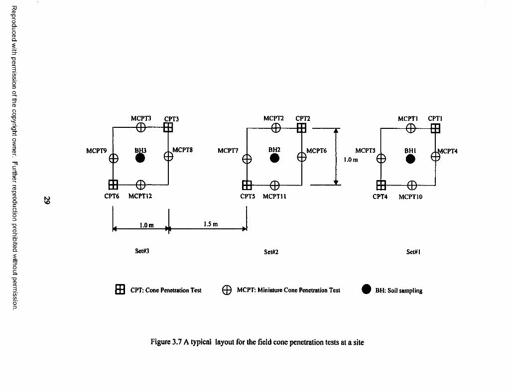
shown in Figure 3.7, a typical cone penetration test consists o f three sets at each site.
Undisturbed soil samples were collected using shelby tubes at different depths (up to top
3 m from the surface). Two or three shelbytube samples were retrieved from a borehole.
After the samples being retrieved, both ends of the shelby tubes were sealed with
polyethylene covers. Then soil samples were extracted from the shelby tubes, they were
sealed and stored in a constant humidity room for laboratory testing. This procedure
ensures the same in-situ moisture content in the samples during their transportation and
handling. Both soil sampling and cone penetration tests were performed in the same day
to ensure similar conditions. This procedure minimizes the difference between field and
laboratory testing parameters in terms of moisture content and unit weight.
3 3 i Laboratory Soil Property Testing
Particle size distribution, Atterberg limits, water content, specific gravity, and
standard Proctor compaction tests were performed. At different confining pressures,
drained and undrained triaxial tests were performed. These tests are used to obtain the
shear strength parameters, cohesion intercept and effective friction angle.
3.4 Laboratory Cone Penetration Testing
This section presents the methodology used in the laboratory cone testing
program. The details of the equipment used in this study are also described. The
equipment includes the cone penetration test system used for the laboratory cone testing
program.
3.4.1 Introduction
The AASHTO guide for design of pavement structures (1993) stipulates that
laboratory resilient modulus tests be performed on representative subgrade soil samples
28
Reproduced with permission of the copyright owner. Further reproduction prohibited without permission.
Reproduced
with perm
ission of the
copyright ow
ner. Further
reproduction prohibited
without
permission.
MCPT3 CPT3 MCPT2 CPT2 MCPT1 CPT1
toso
MCPT8BH3MCPT9
CPT6 MCPT12
i i
BH2MCPT7 MCPT5MCPT6 BHl 1CPT41.0 m
CPT5 MCPT11 CPT4 MCPT10
1.0 m k l.S mH...... "'V r"“ .... "w*
Set#3 Set#2 Set# I
f f l CPT: Cone Penetration Test @ MCPT: Miniature Cone Penetration Test ^ BH: Soil sampling
Figure 3.7 A typical layout for the field cone penetration tests at a site

in different moisture seasons in a year, such as rainy and dry, to estimate the seasonal
resilient modulus values. This procedure quantifies the relative damage in a pavement
during each moisture season in a year. The relative damage is taken into account in the
pavement design. From the relative damage, an effective design resilient modulus value
is estimated. In addition to estimating the seasonal modulus values, the AASHTO guide
for design of pavement structures states that a year be divided into different time intervals
during which the estimated seasonal resilient modulus values are effective. The
minimum time interval might not be less than one-half month for any season. In this
procedure, the seasonal resilient modulus values are assigned in their corresponding time
periods. Then the seasonal resilient modulus values must be converted to the effective
design resilient modulus value with the aid of the charts or equations given in the
AASHTO guide for design of pavement structures. For rigid pavements, the resilient
modulus of subgrade must be converted into an effective modulus of subgrade reaction
(k-value) with the aid of the charts or equations given in the AASHTO guide for design
of pavement structures.
In the field, a subgrade soil encounters wetting and drying cycles. The subgrade
resilient modulus increases as soil dries out in the field. In the field, the resilient modulus
is expected to decrease in a wet period. Therefore, the laboratory resilient modulus test
should be performed on samples taken in wet seasons and dry seasons since they change
the subgrade soil resilient modulus. Both the resilient modulus and cone penetration test
parameters are affected by the moisture content and unit weight of soils. Due to these
facts, duplicating the moisture cycle is important. As given in Table 3.3, a laboratory
cone penetration testing program was performed to study the effect of moisture content
30
Reproduced with permission of the copyright owner. Further reproduction prohibited without permission.
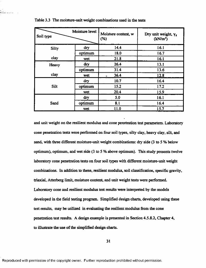
Table 3.3 The moisture-unit weight combinations used in the tests
Moisture level Soil type ---- Moisture content, w
(%)Dry unit weight, Yd
(kN/m3)
Silty dry 14.4 16.1optimum 18.0 16.7
clay wet 21.8 16.1Heavy dry 26.4 13.1
optimum 31.4 13.6clay wet - 36.4 12.8
dry 10.7 16.4Silt optimum 15.2 17.2
wet 20.4 15.9dry 5.0 16.1
Sand optimum 8.1 16.4wet 11.0 15.7
and unit weight on the resilient modulus and cone penetration test parameters. Laboratory
cone penetration tests were performed on four soil types, silty clay, heavy clay, silt, and
sand, with three different moisture-unit weight combinations: dry side (3 to 5 % below
optimum), optimum, and wet side (3 to 5 % above optimum). This study presents twelve
laboratory cone penetration tests on four soil types with different moisture-unit weight
combinations. In addition to these, resilient modulus, soil classification, specific gravity,
tri axial, Atterberg limit, moisture content, and unit weight tests were performed.
Laboratory cone and resilient modulus test results were interpreted by the models
developed in the field testing program. Simplified design charts, developed using these
test results, may be utilized in evaluating the resilient modulus from the cone
penetration test results. A design example is presented in Section 4.5.8.2, Chapter 4,
to illustrate the use o f the simplified design charts.
31
Reproduced with permission of the copyright owner. Further reproduction prohibited without permission.

3.4.2 Objectives
• The main objective in this study was to evaluate the effect of variation in the
moisture and unit weight on the predicted resilient modulus from the cone
parameters.
• Verify the models which were developed using the field cone penetration and
corresponding resilient modulus testing results.
• Develop simplified design charts to evaluate resilient modulus from the cone
penetration test results.
3.43 Methodology
In order to achieve the objectives, an experimental setup was constructed at
Louisiana Transportation Research Center (LTRC) to perform the laboratory cone
penetration tests. Effects of moisture content, dry unit weight, and soil type were studied.
Dining the cone penetration tip resistance, sleeve friction, and penetration depth were
recorded continuously by the data acquisition system.
3.4.4 Equipment for the Laboratory Cone Test
As shown in Figure 3.8, this experimental setup consists of a 55 gallon metal
rigid wall container, 572 mm in diameter and 864 mm in height, reaction frame of 1130
mm in height and 1525 mm in width, loading frame, hydraulic loading system, 2 cm2
miniature cone penetrometer, depth encoder system, cone pushing and grabbing system,
control box, computer, and data acquisition system. Special straight push rod with a
length of 1800 mm was made for this purpose and attached to the 2 cm2 miniature cone
for continuous intrusion. The hydraulic pushing system, mounted on a metal frame
above the soil sample, consists o f dual piston, double acting hydraulic jacks on a
32
Reproduced with permission of the copyright owner. Further reproduction prohibited without permission.

Hydraulic pushing system
Miniature cone penetrometer
Depth encoder
Reaction frame
Soil sample
Figure 3.8 The laboratory cone test setup
33
Reproduced with permission of the copyright owner. Further reproduction prohibited without permission
collapsible frame. A single stroke of the pushing system is 640 mm. This stroke is
enough to penetrate a soil sample, used in this study, continuously at a rate of
20 mm/sec,. An electronic analog to digital converter depth decoding system is
employed to measure the depth at 4 mm intervals.
3.4.5 Data Acquisition System
The data acquisition system (Tumay, 1997) is depicted in Figure 3.9. The data
acquisition system consists of a Pentium II computer collecting data from the cone
penetrometer through the DGH modules, made by the DGH corporation, Manchester,
New Hampshire. All of the DGH modules are connected to a conversion box via RS485.
The conversion box allows output of RS232 for serial line communication with the
computer. The DGH modules are connected to different channels in the cone penetration
system, such as depth encoder and strain gauges of tip and sleeve. The first DGH
module, D1622, is a pulse counter which is connected to the depth encoder. Other two
channels are DGH modules D1102 which measure voltage with a precision of ±10 mV.
These two are connected to the strain gauges of the tip and sleeve.
3.4.6 Testing Program
3.4.6J Soil Compaction
Disturbed soils o f heavy clay, silty clay, and silt, and sand, were collected by
digging the corresponding soil sites and they were dried in the oven. Soil property tests,
such as moisture unit weight relationship, hydrometer, soil classification, specific gravity,
Atterberg limit tests, and triaxial, were performed on these soils to characterize them.
The standard Proctor test was performed to establish the moisture content-density
relationship for each soil. The optimum moisture content and m axim um dry unit weight,
34
Reproduced with permission of the copyright owner. Further reproduction prohibited without permission.

DB-15 Mini Cone Connection
DGH Module * I DI622
EVENT COUNTER
RS48S
0009
Depth Encorder
Power Red Power • Block
Depth encorder• DtVEV
G <!«*■Power +R +VSPower - Block B GND
Power + Red
Power • BlackDGH Module#2 Dl 102
VOLTAGE
H - 10 mV0 DIW EVDCXVLO
RS485
G due*R *VSB GND
DGH Module#} D t 102Sleeve+•*IH IN
0 D0I/ HI 0 D10/EV
DOO/LO
VOLTAGE
* / - lOmV
Dffanlr • rdtfa
GiUta* R »VS
0 B GNDG< ata-
BAUD RATE 38-4K RS232IN
t10-30 V C ND
To Computer
DB-9 Computer Serial Port RS48S IN
RS48S OUT
Figure 3.9 The data acquisition system for the miniature cone penetration(after Tumay, 1997)
35
Reproduced with permission of the copyright owner. Further reproduction prohibited without permission.

obtained from the standard Proctor tests, of each soil type are given in Chapter 4,
Tables 4.1 and 4.8. For the soil compaction in this testing, three moisture content-unit
weight levels of the moisture- unit weight curve were selected. These are dry side (about
3 to 5 % below the optimum), optimum, and wet side (about 3 to 5 % above the
optimum). The selected moisture content-unit weight levels are given in Table 3.3.
First, dry soils were pulverized and sieved through No. 4 (4.75 mm) sieve. Second, the
weight of the soil, passing No. 4 sieve, at the required water content, to be compacted into
the volume of the container to obtain the required density, was calculated. After
establishing the number of layers to be compacted in the container, soil was mixed with
the required amount of water in a mixing pan. After placing the required amount of wet
soil for the first layer in the container, it was compacted until the required height was
achieved. Fine-grained soil was compacted using an electric jack hammer, whereas
coarse-grained soil was compacted using an electric vibrator. A certain selected pattern
of compaction was followed. While the compactor compacting, it moved on the soil
surface very closely in a circular path starting from the center of the soil sample so that
every where in the soil surface was compacted uniformly. Then the compactor moved to
the adjacent circular path and compacted the soil. This procedure continued until the
compactor reached the rigid wall of the container. This path was reversed and this
procedure was repeated until the required height was achieved. In this way, a uniform
compaction effort was applied on the soil layer.
In order to determine the layer thickness, several compaction trials were
performed with different layer depths. The results varied between 100 mm to 150 mm.
After these compaction trials, each layer thickness in compaction was maintained at
36
Reproduced with permission of the copyright owner. Further reproduction prohibited without permission.

125 mm. At least six layers were used for soil compaction. After compacting each layer,
the top of the surface was scarified. This compaction procedure was repeated for the
other layers.
3.4.6.2 Cone testing
After compacting soil in the container, the cone penetration test was performed
with the miniature cone penetrometer. The test layout, as shown in Figure 3.10, was used
in the laboratory cone test. Table 3.4 presents the summary of the testing program. Since
the diameter of the miniature cone penetromer, used in this test, is 15.88 mm, this test
layout allows to maintain a diameter ratio larger than 15 as explained in Section 4.5.2 in
Chapter 4. This test layout was selected to avoid the boundary effects. Cone penetration
tests were performed continuously using a 2 cm2 miniature cone penetrometer.
3.4.63 Soil testing
After the cone penetration test, soil samples were collected at different depths of
the container for the laboratory resilient modulus and soil property tests. For silty clay,
heavy clay, and silt, sand cone tests, LADOTD TR 401-95, were performed at different
depths to obtain the unit weight of soil. First the metal cone was calibrated with clean,
dry, fine sand passing the No. 10 (2 mm) sieve and retained on the No. 50 (0.3 mm)
sieve. In the calibration process of the metal cone, unit weight and weight of fine sand
which filled the metal cone were obtained. The sand cone jar was filled with clean dry
fine sand and weighed. At the selected depths in the soil sample, a leveled surface was
prepared for the sand cone testing. Then the sand cone jar with valve closed was inverted
and placed on the prepared surface. After placing the sand cone firmly against the
prepared surface, opened the valve and let fine sand flow to a stop. Then closed the valve
37
Reproduced with permission of the copyright owner. Further reproduction prohibited without permission.
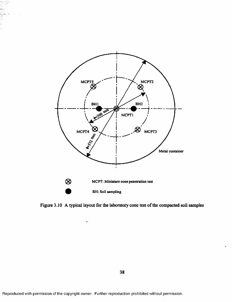
MCPT2MCPT5
BH2 .
— # ■ — f -MCPT1
BH1
MCPT4 MCPT3
Metal container
<8> MCPT: Miniature cone penetration test
BH: Soil sampling
Figure 3.10 A typical layout for the laboratory cone test of the compacted soil samples
38
Reproduced with permission of the copyright owner. Further reproduction prohibited without permission.

Table 3.4 Laboratory cone testing program
Soil type Tests No. of tests
PRF-silty clay CIMCPT: 5
Soil sampling: 2
PRF-heavy clay CIMCPT: 5
Soil sampling: 2
PRF-silt CIMCPT: 5
Soil sampling: 2
Sand CIMCPT: 5
Soil sampling: 2
Legend: CIMCPT- Continuous intrusion Miniature Cone Penetration Test,
Soil sampling- Soil samples retrieved from the boreholes
39
Reproduced with permission of the copyright owner. Further reproduction prohibited without permission.

and weighed the sand cone jar. Then the weight of fine sand in the metal cone was
estimated. After removing all fine sand from the prepared surface, a small hole was
prepared in the center of the original position of the sand cone by excavating soil. The
excavated soils were carefully collected without losing any part of them. The weight of
the excavated soil was measured. Then the sand cone jar with valve closed was inverted
and placed on the prepared hole such that the metal cone covered the open area of the
hole. After placing the sand cone firmly against the prepared surface, opened the valve
and let fine sand flow to a stop. The valve was closed and the sand cone jar was
weighed. The weight of the fine sand, filled the excavated hole, was estimated. Then the
volume of the excavated hole was estimated. The excavated soil was dried and weighed.
Next, the unit weight of the excavated soil was estimated. The excavated soil was
subjected to the moisture content evaluation. This procedure was repeated at each
selected location in the soil sample. In this way, moisture and unit weight profile of the
compacted soil in the container was established. Due to the relatively small dimensions
of the compacted soil sample, the nuclear density test may not be suitable in this study.
Unfortunately, the balloon test was not available for this study.
3.4.6.4 Resilient Modulus Testing
Resilient modulus tests were also performed on the compacted soil samples.
These resilient modulus tests represent the corresponding moisture-unit weight
combination at the cone penetration tests. According to the AASHTO T-294 test
procedure, laboratory compacted soil samples, at the corresponding moisture unit weight
combination of the cone penetration tests, were used for the resilient modulus testing.
The laboratory cone test results were used to validate the proposed models.
40
Reproduced with permission of the copyright owner. Further reproduction prohibited without permission.

CHAPTER 4
ANALYSIS OF RESULTS
This chapter presents the results of the field and laboratory tests. Soil
characterization of the tested soils is described. The repeatability of the continuous
intrusion miniature cone penetration test results is analyzed. The cone and resilient
modulus test results are analyzed. The models to predict the resilient modulus from the
cone penetration test results are developed. Preliminary design charts are proposed but
not verified due to lack of data. Sensitivity of the pavement design equation is analyzed.
4.1 Soil Characterization
Both the resilient modulus and the cone penetration test results depend on the soil
type and its properties. Therefore, soil characterization is also performed to identify the
soil variables which are important for both testing. Tables 4.1 and 4.2 present the
properties of the soils used in this research.
4.1.1 Pavement Research Facility
The Pavement Research Facility (PRF) is located at Port Allen, Louisiana. This
is the experimentation test site for the Louisiana Transportation Research Center. The
PRF site was selected for the field testing due to the availability of two types of cohesive
soils, heavy clay and silty clay. This site comprises a natural soil deposit of heavy clay
(CH) with 84 percent clay and 14 percent silt. A 1.52 m thick silty clay embankment was
constructed at this site. The PRF-silty clay is classified as CL-ML (silty clay) in the
unified soil classification system, USCS, and A-4 (silty soil) in the AASHTO
classification system. To separate the heavy clay subgrade, a soft soil, and silty clay
embankment, a geotextile fabric was installed.
41
Reproduced with permission of the copyright owner. Further reproduction prohibited without permission.

Table 4.1 Properties of fine-grained soils used in the investigation
Soil site
Property
PRF-Siltyclay
PRF-Heavyclay
1-10/LA-42Clay
LA-15Clay
LA-89Siltyclayloam
SiegenLaneClay
Passing sieve #200 (%) 93 98 90 98 91 98
Clay (%) 23 84 42 44 26 33
Silt (%) 70 14 48 54 65 65
Organic content (%) 4.7 9.2 8 NA NA NA
Liquid limit (LL) (%) 28 93 50 52 34 35
Plastic limit (PL) (%) 22 27 16 25 23 23
Plasticity index (PI) 6 66 34 27 11 12
Specific gravity (GJ 2.67 2.68 2.69 2.70 2.69 2.69
Angle of friction (<j>) (°) 22.0 14.0 28.5 14.0 17.0 19.2
Optimum water content ( w ^ (%)
18.0 31.4 18.1 28.1 20.2 17.5
Maximum dry unit weight (YdnaJ (kN/m3)
16.7 13.6 16.8 15.1 16.5 17.0
Soil classification (USCS)
CL-ML(Siltyclay)
CH(Fatclay)
CH(Fatclay)
CH(Fatclay)
CL(Leanclay)
CL(Leanclay)
Soil classification (AASHTO)
A-4(Siltysoil)
A-7-6(Clayey
soil)
A-7-6(Clayey
soil)
A-7-6(Clayey
soil)
A-6(Siltyclay
loam)
A-6(Siltyclay)
42
Reproduced with permission of the copyright owner. Further reproduction prohibited without permission.

Table 4.2 Properties of coarse-grained soil used in the investigation
PropertySoil site LA-1
SandLA-28Sand
Passing sieve #200 (%) 5 30
Clay (%) 5 12
Silt (%) 0 18
Organic content (%) NA NA
Liquid limit (LL)(%) NA NA
Plastic limit (PL) (%) NA NA
Plasticity index (PI) NA NA
Specific gravity (GJ 2.69 2.68
Angle of friction (<(►) (°) 28 28
Optimum water content ( w ^ (%)
14.4 11.4
Maximum dry unit weight fa __) (kN/m3) 16.3 18.3
Soil classification SP-SM SM(USCS) (Poorly
graded sand with silt)
(Silty sand)
Soil classification (AASHTO) A-3 (fine sand)
A-2-4 (Silty sand)
43
Reproduced with permission of the copyright owner. Further reproduction prohibited without permission.

The PRF-heavy clay is a very soft material. According to soil tests, this clay
consists of medium gray soft normally consolidated clay with traces of organic materials
and iron oxide. The PRF-heavy clay is classified as CH (fat clay) in the USCS and A-7-6
(clay) in the AASHTO classification system.
4.1.2 State Route LA-42 (Highland Road) at 1-10
This site is located at the intersection of the State Route LA-42 (Highland Road)
and the Interstate I-10, Baton Rouge, Louisiana. The laboratory soil test results showed
that this soil consists of the brownish gray fissured stiff overconsolidated clay. Chen and
Mayne (1994) performed a detailed soil sampling and cone penetration testing at this site
up to 34 m. The soil is classified as CH (fat clay) in the USCS and A-7-6 (clay) in the
AASHTO classification system.
4.13 State Route LA-15
The LA-15 test site is located in Concordia Parish about 15 miles south of
Vidalia. The site is a part of the Mississippi River Levee. This is also located at the up
slope of the LA-15. The soil is classified as the A-7-6 (clayey soil) using the AASHTO
classification.
4.1.4 State Route LA-89/ New Iberia
The LA-89 site is located in New Iberia. The site consists of lime treated recycled
soil-cement base. The subgrade soil is classified as CL (lean clay) in the USCS
classification and A-6 (silty clay loam) in the AASHTO classification system.
4.1.5 Siegcn Lane/ Baton Rouge
The Siegen Lane test site soil is classified as CL (lean clay) in the USCS
classification and A-6 (silty clay) in the AASHTO classification system.
44
Reproduced with permission of the copyright owner. Further reproduction prohibited without permission.

4.1.6 State Route LA-28/ Simpson
The LA-28 site is located in Simpson. Vernon Parish. This site is used as a
borrow pit for the roadway embankment construction by the Louisiana Department of
Transportation and Development. The soil at this site is coarse-grained soil. The soil is
classified as SM (silty sand) in the USCS classification and A-2-4 (silty sand) in the
AASHTO classification system. Shear strength parameters for this soil was estimated
from Das (1983).
4.1.7 State Route LA-1/ Larose
This site is located on LA-1 in Larose, Lafourche Parish. This is an embankment.
The soil at this site is coarse-grained soil. SP-SM (poorly graded sand with silt) in the
USCS classification and A-3 (fine sand) in the AASHTO classification system. Shear
strength parameters for this soil was also estimated from Das (1983).
4.2 Cone Test Results
The CIMCPT is a newly developed system. The miniature friction cone is to be
calibrated with respect to the 15 cm2 cone in different soil types. Cone penetration tests
were performed according to Table 3.2 in Chapter 3 in order to ensure the reliability and
repeatability of the miniature cone penetration test data.
The field testing layout for the PRF-silty clay is given in Figure 4.1. Twelve
CEMCPTs and three CPTs were performed. Soil samples were also obtained for the
laboratory testing, as described in Section 3.3.4. The field tests were performed in three
sets. The cone penetrated to a depth of 2 m. Figure 4 2 depicts the cone penetration test
results for the PRF-silty clay for field test set 1. According to Figure 4.2, in the 0.3 m
limestone base, the tip resistance of the miniature cone penetrometer fluctuates due to its
45
Reproduced with permission of the copyright owner. Further reproduction prohibited without permission.

Reproduced
with perm
ission of the
copyright ow
ner. Further
reproduction prohibited
without
permission.
MCPT12 MCPT8 MCPT3
CPT3MCPT9MCPT10
BH3CPT6 MCPT11
MCPT1CPT2 CPT1MCPT6 MCPT2MCPT51.0 m
BH1BH2MCPT7 CPT4 MCPT4
4*.ON g 1.0 m , 1.5 mi----------------------------------n
Set#3 Set#2 Set# I
f f l CPT: Cone Penetration Test MCPT: Miniature Cone Penetration Test BH: Soil sampling
Figure 4.1 Field test layout for the PRF-Silty clay site

mottnm coatMM • 4 2H utsttu danaty "22.1 kN/n»* % PHautg Mv« no. 4 • 23
S«tty day (ambaakimM) LiqUd Lumt" 21 Phottaiy (ndax • 6 Group Indax >1 HPausog J200 mvo • 93 Oi|Wic content • 4 7% Clasuficaoon.AASHTO- A-4 USCS: CL-ML
Goouxalt ftbnc fora
Heavy day (sutural (fcpont) Liquid Lumt• 93 Rwmiy Indn * 66 Group Indm " 16 % P w ng »200 e m * 9* Organic coolant • 9 2S AASHTO A-7*6 USCS CH
0.0
0.4
0.8
■s&Q
1.2
2.0
M Crr l
— M O T !
— MCPT4
1.6 h _
1 1 1 . l U
0 10 20 30 40 0 .0 0 .1 0 .2 0 .3 0 .40 .5
Tip resistance, qc (MPa)
Sleeve friction, fs (MPa)
Figure 4.2 Cone penetration test results of the PRF-silty clay (set #1)
47
Reproduced with permission of the copyright owner. Further reproduction prohibited without permission.
high sensitivity. In this layer, the tip resistance recorded by the m iniature cone is higher
than that of the CPT. In general, the tip resistance of the miniature cone penetration test
is slightly higher than that of CPT (Tumay et al., 1997 and 1998). But the sleeve friction
of the miniature cone penetration test is slightly lower than that of CPT. This observation
was also made by Tumay et al., (1997 and 1998). This is attributed to the scale effect of
the miniature cone penetrometer (de Lima and Tumay,1991 and Tumay et al., 1997 and
1998). The miniature cone penetration generates a smaller pressure bulb than the CPT
does. Therefore, the miniature cone penetration identifies thin soil layers. In the silty
clay embankment, a fine-grained soil layer, both CPT and CIMCPT results exhibit
similar patterns indicating the verification of the implementation of the CIMCPT system.
Several studies (Tumay et al., 1997 and 1998; FCurup and Tumay, 1999;
Mohammad te al., 2000; Titi et al., 2000) have shown the reliability and repeatability of
the CIMCPT test results. A statistical analysis was performed on the cone test results to
determine the coefficient of variation. In a data set, average the CIMCPT test results
along the depth and estimate the standard deviation as well as coefficient of variation.
The average value of all the CIMCPT test results in a data set at a selected depth is
considered for the resilient modulus evaluation from the cone penetration test results.
The coefficient of variation of CIMCPT results of silty clay is shown in Figure 4.3. A
high variation of tip resistance, as shown in Figure 4.3, was observed in the top layer of
this site which consists of a gravel base of 03 m. But below the top 0.3 m, only a small
variation among the CIMCPT results can be observed.
Figure 4.4 presents the field testing layout for the PRF-heavy clay. Out o f eight
CIMCPTs five were satisfactory while the other three were erroneous due to the
48
Reproduced with permission of the copyright owner. Further reproduction prohibited without permission.

Depth
(m
)
0 .0
0.4
Siltyj clay
0.8
1.2
1.6
2.00 40 80 120
COV of qc (%)
0 40 80 120
COV of fs (%)
0 40 80 120 160
COV of Rf (%)
Legend: qc - Tip resistance, £ - Sleeve friction, Rf - Friction ratio
Figure 4.3 Coefficient of variation of CIMCPT for the cone test of the PRF-silty clay
49
Reproduced with permission of the copyright owner. Further reproduction prohibited without permission.
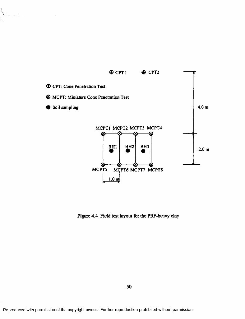
© CPT1 © CPT2
© CPT: Cone Penetration Test
® MCPT: Miniature Cone Penetration Test
© Soil sampling 4.0 m
MCPT1 MCPT2 MCPT3 MCPT4
BH2 BH3BH1
MCPT5 MCPT6 MCPT7 MCPT8
1.0 m
2.0 m
Figure 4.4 Field test layout for the PRF-heavy clay
50
Reproduced with permission of the copyright owner. Further reproduction prohibited without permission.

malfunction in the data acquisition system. Therefore, only five of the eight CIMCPTs
(test Nos. 1 ,3 ,5 ,6 , and 8) were used in the data analysis. Figure 4.5 depicts the cone
penetration test results for the PRF-heavy clay for field test setl. The miniature cone
recorded low tip resistance and high sleeve friction due to soft clayey nature of this soil.
The coefficient of variation of the test results is depicted in Figure 4.6. According to the
testing layout, shown in Figure 4.4, a high coefficient of variation in heavy clay may be
attributed to the soil variability resulting from the difference in the distance among the
test locations of CIMCPTs. The soil deposit may not be homogeneous in all the test
points.
Figure 4.7 presents the field testing layout for the LA-42/1-10 site. Figures 4.8
depicts the cone penetration test results. The top layer (0 to about 0.5 m) forms with a
stiff, desiccated deposit. Therefore, the tip resistance showed high variability in the top
layer. The following soil deposit is a heavily overconsolidated, desiccated silty clay/
clayey silt with occasional sand pockets (Chen and Mayne, 1994). When the miniature
cone penetrometer encounters a sand pocket, a high tip resistance was expected. Below
the top layer, the CPT and CIMCPT soundings reflect the similar patterns with different
magnitudes. Figure 4.9 shows the coefficient of variation of the tip resistance and the
sleeve friction. A large deviation of the cone test results can be observed in the top layer.
Below the top layer, a small deviation of the cone test results can be observed. The
average COV of the tip resistance is 18.5 percent for the miniature cone whereas, that is
12.5 percent for the 15 cm2 cone. The average COV of the sleeve friction is 18.2 percent
for the miniature cone whereas, that is 16 percent for the 15 cm2 cone. Because of the
high sensitivity of the miniature cone and its capability to identify thin soil layers, the
51
Reproduced with permission of the copyright owner. Further reproduction prohibited without permission.

Depth
(m
)
0 .0
0.5
1.0
1.5
Heavy clay2.0
0.0 1.0
qc(MPa)
2.0 0.0
(MPa)
0.1
M CPTl MCPT5 MCPT6 CPT I
!
20 400
Legend: q,. - Tip resistance, f5 - Sleeve friction, Rf - Friction ratio
Figure 4.5 Cone penetration test results of the PRF-heavy clay (set #1)
52
Reproduced with permission of the copyright owner. Further reproduction prohibited without permission.

0 .0
0.5
s
tuo
2.0100500 50.00.0 100.0
COV of Tip resistance, qc(%) COV of Sleeve friction, fs (%)
Figure 4.6 CoefBcient of variation of CIMCPT for the cone test of the PRF-heavy clay
53
Reproduced with permission of the copyright owner. Further reproduction prohibited without permission.

Reproduced
with perm
ission of the
copyright ow
ner. Further
reproduction prohibited
without
permission.
MCPT10 CPT4
MCPT5BH1MCPT4
CPT1 MCPT1
MCPT14MCPT11 CPT5 MCPTI2 CPT6MCPT13
BH3MCPT6 MCPT8MCPT7 ICPT9
1.0 mBH4BH2
CPT2 MCPT2 CPT3 MCPT3
£ 1.0 m t, 1.5 m4 P 9 ----- pj
Set## 1 Set##2 Set#3 Set#4
f f l CPT: Cone Penetration Test ® MCPT: Miniature Cone Penetration Test ^ BH: Soil sampling
Figure 4.7 Field test layout for the LA-42/1-10 site

Depth
(m
)0 .0
1-10/LA-42
1.0
2.0
3.07 14 0.00 0.15 0.30
qc(MPa) fs (MPa)
x j h t |
J h - £ \
!
i S fc
L 5 I E 3
i ®
&
I
*
NV
\/W >
>
' VjX I
1 ____
0 6 12
Rf(%)
- MCPT5- MCPT6- CPT 2- CPT 4
Figure 4.8 Cone penetration test results of the LA-42/1-10 site (set #1)
55
Reproduced with permission of the copyright owner. Further reproduction prohibited without permission.

Depth
(m
)
0 .0
LA-42/1-10
1.0
2.0
3.0100500
COV of Tip resistance, qc (%)
0 50 100
COV of Sleeve friction, f s (%)
MCPT|CPT
Legend: q,. - Tip resistance, fs - Sleeve friction, Rf - Friction ratio
Figure 4.9 C oefficient of variation for the cone test of the LA-42/1-10 site
56
Reproduced with permission of the copyright owner. Further reproduction prohibited without permission.

coefficient of variation for the CIMCPT sounding is slightly higher than that of the CPT
results, particularly at the top layer (Tumay et al., 1997).
Figure 4.10 presents the field testing layout for the LA-15 site. Figure 4.11
depicts the cone penetration test results. The CPT and CIMCPT soundings reflect the
similar patterns. Due to the scale effects, the tip resistance of the m iniature cone
penetration is slightly higher than that of the CPT (Tumay et al., 1997). The coefficient
of variation of the test results is depicted in Figure 4.12. The coefficient of variation
profiles of both CPT and CIMCPT follow the same pattern. But the coefficient of
variation of the CIMCPT is slightly greater than that of the CPT. This is attributed to the
high sensitivity of the miniature cone penetrometer (Tumay et al., 1997).
Figure 4.13 presents the field testing layout for the LA-89 site. Figure 4.14
depicts the cone penetration test results. The cone penetration results indicate the natural
soil under the subgrade is a soft material as its tip resistance is very low. The CPT and
CIMCPT soundings reflect the similar pattern with different magnitudes. The coefficient
of variation of the test results is depicted in Figure 4.15. In the top layer (0 to about
0.4 m) the coefficient of variation is high due to the high sensitivity of the miniature cone
penetrometer. But the coefficient of variation of CIMCPT results is small in the bottom
layers. The coefficient of variation profiles of both CPT and CIMCPT follow similar
patterns up to top 2 m.
Figure 4.16 presents the field testing layout for the Siegen Lane site. Figure 4.17
depicts the cone penetration test results. The CPT and CIMCPT soundings reflect the
similar patterns with different magnitudes. The coefficient of variation profiles of both
CPT and CIMCPT follow similar patterns (Figure 4.18).
57
Reproduced with permission of the copyright owner. Further reproduction prohibited without permission.

Reproduced
with perm
ission of the
copyright ow
ner. Further
reproduction prohibited
without
permission.
MCPT12 CPT6 MCPT11 CPT5 MCPT10 CPT4
oo
MCPT8BH3MCPT9
CPT3 MCPT3
BH2MCPT7 MCPT6
1.0 m
CPT2 MCPT2
1.0 m * 1.5 mi*"—... 1------- -------- w
MCPT5 ICPT4
CPT1 MCPT11
Set#3 Set#2 Settfl
f f l CPT: Cone Penetration Test ® MCPT: Miniature Cone Penetration Test ^ BH: Soil sampling
Figure 4.10 Field test layout for the LA-15 site

Depth
(m
)
0.0
1.0
2.0
3.02010 0.2 0.40.0
qc (MPa) fs (MPa)
0 6
Rf(%)
- MCPT1- MCPT4- MCPT5- MCPT 10- CPT 1- CPT 4
Figure 4.11 Cone penetration test results of the LA-15 site (set #1)
59
Reproduced with permission of the copyright owner. Further reproduction prohibited without permission.

Depth
(m
)
0 .0
0.5
LA-15 -
1.0
1.5
2.0
2.5
3.0100500 100 10050 0 50 100
COV of qc (%) COV of f- (%) COV of Rf (%)
MCPTCPT
Figure 4.12 Coefficient of variation for the cone test of the LA-15 site
60
Reproduced with permission of the copyright owner. Further reproduction prohibited without permission.
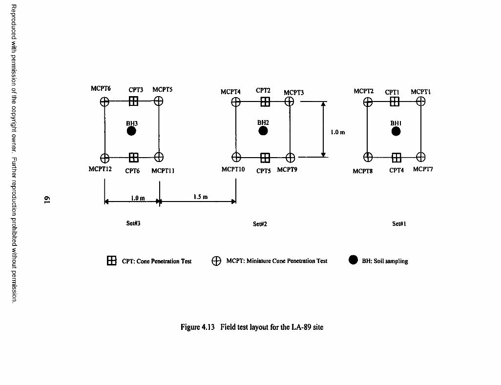
Reproduced
with perm
ission of the
copyright ow
ner. Further
reproduction prohibited
without
permission.
MCPT6 CPT3 MCPT5
BH3
MCPT12 CPT6 MCPT11
MCPT4 CPT2 MCPT3
BH2
MCPT10 CPT5 MCPT9
MCPT2 CPU
® — ffl-
1.0 mBH1
© — E hMCPT8 CPT4
4 1.0 m k. 1.3 m
Set#3 Set#2 Setfll
f f l CPT: Cone Penetration Test ^ MCPT: Miniature Cone Penetration Test ^ BH: Soil sampling
MCPT1
- ©
- ©MCPT7
Figure 4.13 Field test layout for the LA-89 site

Depth
(m
)
0 .0
1.0 ■tjr
2.0
3.01260.2 0.4 010 0.050
q (MPa) fs (MPa) Rf(%)
- MCPT I- MCPT 2- CPT 1- CPT 4
Legend: qe - Tip resistance, 4 - Sleeve friction, Rf - Friction ratio
Figure 4.14 Cone penetration test results of the LA-89 site (set #1)
62
Reproduced with permission of the copyright owner. Further reproduction prohibited without permission.
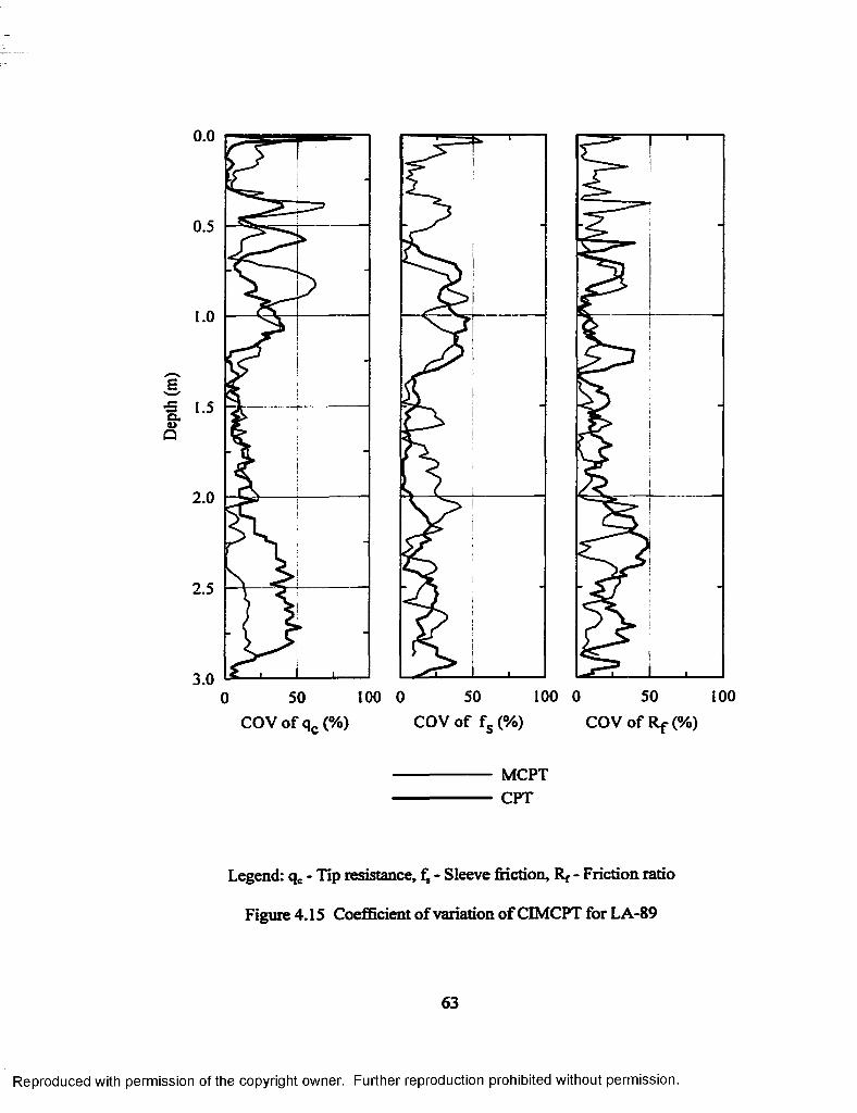
Depth
(m
)
0 .0
0.5
t.O
1.5
2.0
2.5
3.0100100 0500 50 1000
COV of qc (%) COV of fs (%) COV of Rf (%)
----------------- MCPT----------------- CPT
Legend: q,. - Tip resistance, fj - Sleeve Motion, Rf - Friction ratio
Figure 4.15 Coefficient of variation of CIMCPT for LA-89
63
Reproduced with permission of the copyright owner. Further reproduction prohibited without permission.

Reproduced
with perm
ission of the
copyright ow
ner. Further
reproduction prohibited
without
permission.
MCPT3 CPT3 MCPT2 CPT2
MCPT8BH3MCPT9
CPT6 MCPT12
BH2MCPT7 MCPT6
1.0 m
CPT5 MCPT11
MCPT1 CPT1
- ■e ebMCPT5
1.0 m * I.S m1 ................ .... ....Wl
Set#3 Set#2
0BHI
i f
ffl 0 -CPT4 MCPT10
Set# I
f f l CPT: Cone Penetration Test ® MCPT: Miniature Cone Penetration Test ^ BH: Soil sampling
Figure 4.16 Field test layout for the Siegen Lane site
1CPT4

Depth
(m
)
0 .0
1.0
2.0
3.010 20 0.0 0.6 1.2
qc(MPa) f- (MPa)
0 6 12
Rf(%)
Siegen Lane Set-1------------- MCPT I------------- MCPT 4------------- MCPT 5------------- MCPT 10------------- CPT 1------------- CPT 4
Figure 4.17 Cone penetration test results of the Siegen Lane site (set #1)
65
Reproduced with permission of the copyright owner. Further reproduction prohibited without permission.

Depth
(m
)
0 .0
0.5
t.O
1.5
2.0
2.5
3.0100500 1000 50 100500
COV of qc (%) COV of f . (%) COV of Rf (%)
MCPTCPT
Legend: qc - Tip resistance, f, - Sleeve friction, Rf - Friction ratio
Figure 4.18 Coefficient of variation of the CIMCPT for Siegen Lane
66
Reproduced with permission of the copyright owner. Further reproduction prohibited without permission.

Figure 4.19 presents the cone test results of the LA-28 site. The CPT and CIMCPT
soundings reflect the similar patterns. As shown in Figure 4.19, coarse-grained soil, such
as sand, exhibits higher cone tip resistance and low friction ratio than those of fine
grained soil, such as silty clay, as shown Figure 4.2. Fine-grained soil, such as clay,
exhibits low cone tip resistance and high friction ratio. The coefficient of variation of the
test results is depicted in Figure 4.20. The coefficient of variation of the CIMCPT
follows the same pattern as that o f CPT. But the values of coefficient of variation o f the
CIMCPT results are slightly higher than that of CPT. This is due to the fact that high
sensitivity of the miniature cone penetration. The miniature cone penetrometer is capable
of identifying small variation in a soil layer (Tumay et. al, 1997).
The soil at Larose site consists of dense fine sand. In such soil, sand particles will
rearrange their orientation during penetration to let the state of compactness increase
around the cone. The increase of the density of the sand, due to the penetration of the
cone, results in an increase in the soil resistance to the cone penetration. Therefore, a
larger thrust is needed to push the cone into the ground. At Larose site, the maximum
allowable thrust to push the miniature cone was reached with very little advancement of
the cone. Therefore, no CIMCPT were conducted at this site.
Comparison of the CPT data and CIMCPT data for most of the investigated sites has
shown that the cone penetration test parameters and coefficient of variation of the
CIMCPT results follow almost the same pattern as those of CPT. Even though, the
values of the tip resistance and coefficient of variation of the CIMCPT results are
slightly higher than those of CPT, these results imply the verification of the
implementation of the CIMCPT results. This observation was also made by Tumay et al.,
67
Reproduced with permission of the copyright owner. Further reproduction prohibited without permission.
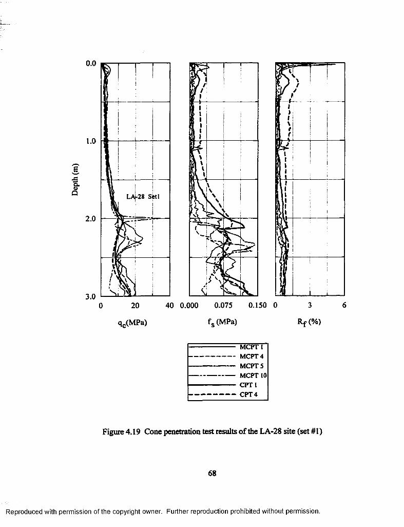
Depth
(m
)0 .0
1.0
2.0
3.0
! LAI-28 Set!
0.150 00.07540 0.000
qc(MPa) f„ (MPa) R f (% )
- MCPT 1 - - MCPT 4- MCPT 5- MCPT 10- CPT 1- CPT 4
Figure 4.19 Cone penetration test results of the LA-28 site (set #1)
68
Reproduced with permission of the copyright owner. Further reproduction prohibited without permission.

Depth
(m
)
0 .0
0.5LA-28
1.0
1.5
2.0
2.5
3.040 80 1200 0 40 80 120 1600 50 100 150
COV of qc (%) COV of fs (%) COV of R f (%)
----------------- MCPT----------------- CPT
Figure 4.20 Coefficient of variation for LA-28 (Set#l)
Reproduced with permission of the copyright owner. Further reproduction prohibited without permission.

(1997), Kurup and Tumay (1999), and Titietal. (2000). Several conversion factors are
available (Tumay et al., 1992; Tumay et al., 1997; Kurup et al., 1999; Mohammad et al.,
2000; Titi et al., 2000) to convert the CIMCPT into the CPT test results. In general, for
fine-grained soil, the tip resistance of the CIMCPT is about 11 percent greater than that of
the 15 cm2 cone and the sleeve friction of the CIMCPT is about 9 percent less than that of
the 15 cm2 cone (Titi et al., 2000).
4 3 Resilient Modulus Test Results
The resilient modulus test was performed with three confining stresses and five
deviator stress levels for each confining stress. The test results of each confining stress
were connected with a linear regression line. This line represents the measured resilient
modulus at different deviator stress levels, expected in the pavements.
Figure 4.21 depicts the laboratory measured resilient modulus, obtained from the
AASHTO T-294 test, for PRF-silty clay. As shown in Figure 4.21, the laboratory
measured resilient modulus increases as the confining pressure increases, whereas it
decreases as the deviator stress increases. This result indicates the stress dependency of
the resilient modulus. This result is consistent with the previous studies (Fredlund et al.,
1977; Ullidtz, 19S7; Nataatmadja et al., 1989; Kamal et al., 1993; Mohammad et al.,
1994; Mohammad et al., 1995; Puppala et al., 1996; Mohammad et al., 1998;
Mohammad et al., 1999). The resilient modulus of the silty clay at depth of 0.8 m is
lower than that at depth of 1.0 m. At 0.8 m, water content and dry unit weight of the silty
clay are 25.4 percent and 15.9 kN/m3, whereas at 1.0 m, those of the silty clay soil sample
are 23.0 percent and 16.5 kN/m3 respectively. At 1.0 m, water content of the silty clay
soil sample is lower than that at 0.8 m. At 1.0 m, dry unit weight of the silty clay soil
70
Reproduced with permission of the copyright owner. Further reproduction prohibited without permission.

100
w= 25.4 %, y„= 15.9 kN/m3 'Silty clay
ui
Confining stress(U
crr =20.7 kPaCOSample depth=0.8 mo . =0.0 kPa
10010
Deviator stress, (kPa)
100w= 23.0 %, yd= 16.5 kN/m3 -Silty clay
Urn
cn
Confining stress
cj_ =20.7 kPaSample depth=l .0 mcr. =0.0 kPa
10010
Deviator stress, ctj (kPa)
Figure 4.21 Resilient modulus of PRF-silty clay at borehole 1
71
Reproduced with permission of the copyright owner. Further reproduction prohibited without permission.

sample is greater than that at 0.8 m. The lower the dry unit weight the lower the resilient
modulus. The lower the moisture content the higher the resilient modulus. The effective
deviator stress in clay decreases and hence the resilient modulus decreases as the
dilational properties increases with the moisture content. These observations were also
made by previous studies (Allen, 1989; McGee, 1989; Monismith, 1989; Mohammad et
al., 1995; Drumm et al., 1997; Mohammad et al., 2000). This is the reason to exhibit
higher resilient modulus values o f the soil sample at 1.0 m depth o f silty clay as
compared to those at 0.8m.
Figure 4.22 shows the the resilient modulus values of the PRF-heavy clay. The
resilient modulus of the PRF-heavy clay is lower than that of the PRF-silty clay. This is
because the heavy clay is a softer material with a higher moisture content and a lower dry
unit weight. The in-situ water contents of the silty clay soil samples vary from 21 to 25
percent, whereas those of the heavy clay soil samples vary from 59 to 65 percent. The
dry unit weights of the silty clay soil samples are also greater than those o f the heavy clay
soil samples. The lower resilient modulus of the heavy clay is attributed to both of these
reasons. Hence, it reflects a lower stiffness resulting a lower resilient modulus. As
shown in Figure 4.22, the resilient modulus values of heavy clay at depth of 0.8 m are not
significantly different from those at depth o f 1.0 m. At 0.8 m, water content and dry unit
weight o f heavy clay are 61.6 percent and 9.9 kN/m3 whereas, at 1.0 m, those are 65.1
percent and 9.9 kN/m3 respectively. Since both the samples showed the same dry unit
weight, a significant difference in the resilient modulus at these high moisture contents
may not be exhibited. Confining pressure also showed a little effect on the resilient
modulus o f the heavy clay at these high moisture contents.
72
Reproduced with permission of the copyright owner. Further reproduction prohibited without permission.

c/lJ33-aoScuGO
100 nw= 61.6 %, yd= 9.9 kN/m-*Heavy clay
10Confining stress
ct. =41.3 kPa
Sample depth=0.8 mct. =0.0 kPa
I 10 100Deviator stress, ct (kPa)
csa*2
h*
2IBJ3S-OOSeu
100
w= 65.1 %, yd= 9.9 kN/m3 ;Heavy clay
10Confining stress
a . =41.3 kPa
ct. =20.7 kPaSample depth=1.0 mct. =0.0 kPa
I10 100
Deviator stress, CTj (kPa)
Figure 4.22 Resilient modulus of P&F-heavy clay at borehole 1
73
Reproduced with permission of the copyright owner. Further reproduction prohibited without permission.

The resilient modulus of the LA-42/1-10 clay at depth of 0.8 m is higher than that
at depth of 1.0 m (Figure 4.23). At 0.8 m, water content and dry unit weight of this clay
are 19.6 percent and 17.2 kN/m3, whereas at 1.0 m, those of this clay are 23.0 percent and
16.5 kN/m3 respectively. At 1.0 m, water content of the LA-42/1-10 soil sample is higher
than that at 0.8 m. At 1.0 m, dry unit weight of the LA-42/1-10 soil sample is lower than
that at 0.8 m. As explained previously, the resilient modulus of the LA-42/1-10 clay at
depth of 0.8 m is higher than that at depth of 1.0 m due to these higher unit weight and
lower water content of the 0.8 m depth soil sample.
The resilient modulus of the LA-15 clay at depth of 0.8 m is higher than that at
depth of 1.0 m (Figure 4.24). At 0.8 m, water content and dry unit weight o f this clay are
24.1 percent and 17.3 kN/m3 whereas, at 1.0 m, those are 23.0 percent and 16.2 kN/m3
respectively. At 1.0 m, water content of the LA-15 soil sample is lower than that at 0.8 m
by 1.1 percent. At 1.0 m, dry unit weight o f the LA-15 soil sample is lower than that at
0.8 m. In this case, the higher resilient modulus at depth of 0.8 m is attributed to the
higher unit weight at this depth. This result indicates that the effect of the dry unit weight
is more significant than that of the water content on the resilient properties o f soil.
Figure 4.25 shows the resilient modulus of the LA-89 clay. The resilient modulus
o f the top soil sample is higher than that of the bottom soil sample. The water content
and dry unit weight o f the top soil sample are 26.8 percent and 16.1 kN/m3 respectively.
In the bottom soil sample, the water content and dry unit weight are 28.6 percent and 15.9
kN/m3 respectively. In the bottom soil sample, the water content is higher than that in the
top soil sample. In the bottom soil sample, the dry unit weight is lower than that in the
top soil sample. Similar to previous explanation, the resilient modulus of the top soil
74
Reproduced with permission of the copyright owner. Further reproduction prohibited without permission.
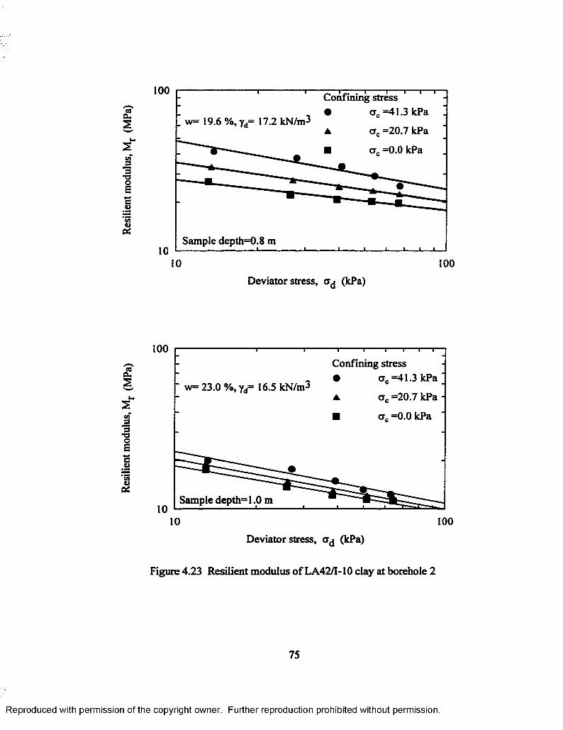
08GUs
i-aoEc<u
100
CT =41.3 kPa .19.6 %, yd= 17.2 kN/m3w =
Ct- =20.7 kPa
ct- =0.0 kPa
Sample depth=0.8 m10
10 100
Deviator stress, ct (kPa)
M3"ST 3OE§sn
100Confining stress
ct-= 41.3 kPa "23.0 %, yd= 16.5 kN/m3w =
ct =20.7kPa -
ct- =0.0 kPa
Sample depth=l .0 m10
10010
Deviator stress, ct (kPa)
Figure 4.23 Resilient modulus of LA42/I-10 clay at borehole 2
75
Reproduced with permission of the copyright owner. Further reproduction prohibited without permission.

03CL*S'w '
ST$3"OOscu
cn<uCd
100w= 24.1 %, yd= 17.3 kN/m3 I
Confining stress
ct, =20.7 kPaSample depth=0.8 mct, =0.0 kPa
1010 100
Deviator stress, ctj (kPa)
C3cu£
cnSTJOS30)tn
{2
100w= 23.0 %, yd= 16.2 kN/m3-
Confining stressct, =41.3 kPa
ct, =20.7 kPaSample depth=1.0 mct, =0.0 kPa
1010 100
Deviator stress, ct (kPa)
Figure 4.24 Resilient modulus of LA-15 clay at borehole 1
76
Reproduced with permission of the copyright owner. Further reproduction prohibited without permission.
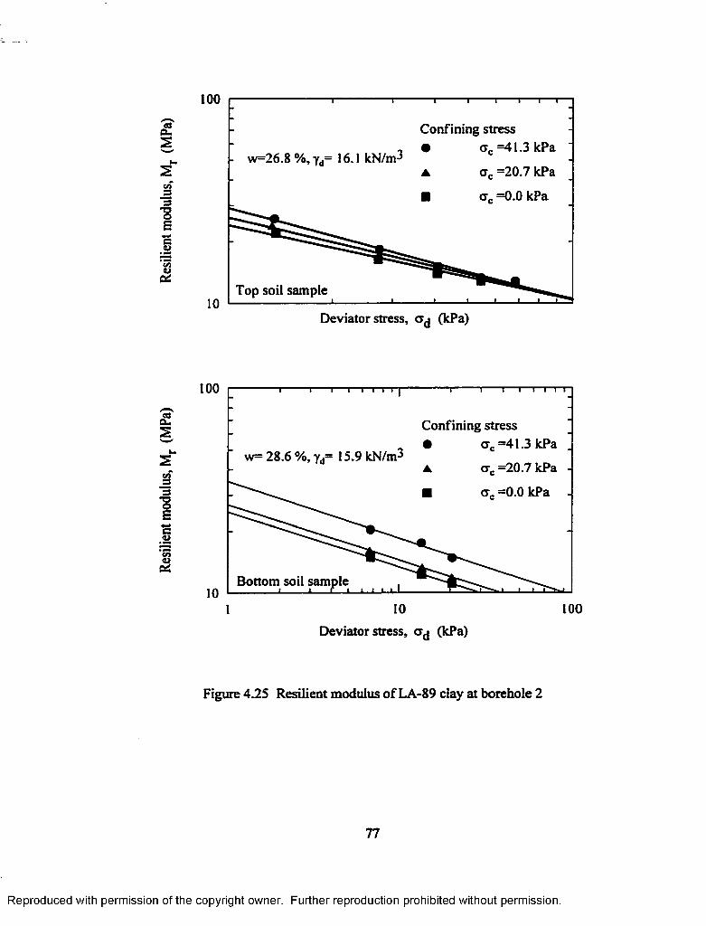
at0L2
Urn
stoJ33•86c<uto0>0*
100
Confining stress
w=26.8 %, yd= 16.1 kN/m3ct. =20.7 kPa
ex. =0.0 kPa
Top soil sample10
Deviator stress, ct (kPa)
ata,2
COs
osc<L>coOed
100
Confining stressex. =41.3 kPa
w= 28.6 %, yd= 15.9 kN/rn^ct. =20.7 kPa
ct. =0.0 kPa
Bottom soil sample10
10 100Deviator stress, ct (kPa)
Figure 4.25 Resilient modulus of LA-89 clay at borehole 2
77
Reproduced with permission of the copyright owner. Further reproduction prohibited without permission.

sample is higher than that in the bottom soil sample due to these higher unit weight and
lower water content o f top soil sample.
Figure 4.26 depicts the resilient modulus of the Siegen Lane clay. The resilient
modulus of the top soil sample is higher than that of the bottom soil sample. In the top
sample, water content and dry unit weight of this clay are 9.5 percent and 18.3 kN/m3,
whereas in the bottom sample, those are 22.5 percent and 17.1 kN/m3 respectively. The
water content of the bottom soil sample is higher than that of the top soil sample. In the
bottom soil sample, dry unit weight of the soil sample is lower than that in the top soil
sample. Similar to previous explanation, the resilient modulus of the top soil sample is
higher than that of the bottom soil sample due to these higher unit weight and lower water
content of i t The top layer (0 to about 0.5 m) of the Siegen Lane site consists a stiff,
desiccated deposit The water content of this top layer is 9.5 percent with respect to the
optimum water content o f 17.5 percent. As shown in Figure 43, the resilient properties of
this soil at low confining stresses exhibited a little deviation from the behavior of fine
grained soils due to the dry and desiccated nature of the top soil layer.
As shown in Figure 4.27, for coarse-grained soil at LA-28 site, the resilient
modulus increases with the bulk stress and confining stress. This is also a typical
behavior of sands. This result is also consistent with the previous studies (Rada et al.,
1981; Mohammad et al., 1994; Mohammad et al., 1998; Mohammad et al., 1999). As the
bulk stress increases stiffness of coarse-grained soil increases. As the confining stress
increases dilational properties decreases. Appendix A presents the resilient modulus test
results. A laboratory resilient modulus test on the field soil samples covers a range of
possible confining and deviator stress levels which are expected under various
78
Reproduced with permission of the copyright owner. Further reproduction prohibited without permission.

«22
ioo
s■cto6cuIA
Confining stress
1010
crc =41.3 kPa
<rc =20.7 kPa w= 9.5 %, yd= 18.3 kN/m3
ctc =0.0 kPa Top soil sample_i___ i ■ ■ ■
100
De viator stress, <rd (kPa)
100/«—s CO 0U2
tn SST3OE Confining stress
a . =41.3 kPaw= 22.5 %, yd= 17.1 kN/m3
Bottom soil sample
Mct =20.7kPa
ct. =0,0 kPa
10010Deviator stress, CTd (kPa)
Figure 4.26 Resilient modulus of Siegen Lane clay
79
Reproduced with permission of the copyright owner. Further reproduction prohibited without permission.

£s
sc/Ts
oEctn
1000Sample depth = 0.8 m
100
Confining stress
a , =20.7 kPa ❖ <rc =103.4 kPa
<tc =34.5 kPa + ctc =137.8 kPa
crc =68.9 kPa10
100 1000
Bulk stress, a b (kPa)
Figure 4.27 Resilient modulus of LA-28 sand
80
Reproduced with permission of the copyright owner. Further reproduction prohibited without permission.

in-situ and traffic stress conditions. As explained in Figure 4.28, the depth o f the soil
sample retrieved from the field is used to estimate the in-situ stresses. Based on the in-
situ stress levels, a corresponding resilient modulus, denoted as the field resilient
modulus, can be interpolated from the laboratory resilient modulus test results.
Figure 4.28 illustrates the interpolation procedure used in this study. Tables 4.3 and 4.4
contain the summary of the field and laboratory test parameters. The moduli of elasticity
(E) were estimated from the laboratory repeated load triaxial testing. By averaging two
or more in-situ resilient modulus values o f a soil type in Table 4.4, the modulus of
elasticity was estimated. The poisson’s ratio (v) was assumed. Table 4.5 contains the
elastic properties o f soils.
4.4 Model Development
In this portion of the study, an attempt was made to establish models to predict the
resilient modulus from the cone penetration measurements. The cone penetration,
resilient modulus, and soil property test results were used in the model development. The
main variables, affecting the resilient modulus from the cone penetration parameters were
identified. The main parameters considered in these models are the soil type, tip
resistance, sleeve friction, resilient modulus, moisture content, dry unit weight, deviator
stress, and confining stress. Since this study aimed to use the CIMCPT in subgrade soil
characterization, its data was used in the model development The CPT data is to be
converted to the CIMCPT data before using the following models.
From Tables 4.3 and 4.4, test results of silty clay and heavy clay were selected for
fine-grained soil models. Before the regression analysis, the variables were arranged to
satisfy several physical conditions.
81
Reproduced with permission of the copyright owner. Further reproduction prohibited without permission.

£s
cn3■aoB++cVcac2
100In-situ confining stress level
In-situ resilient modulus, Mrinjil
Confining stress
=20.7 kPaIn-situ deviator stress,dinsini ct- =0.0 kPa
10 100Deviator stress, od (kPa)
Ground level
T - - - - - - - - - - - - - - - - - - - - - - - - - -Vertical stress, <rv = y h
4Depth, h (m)
± -
Deviator stress, - o» - oc
y - Unit weight o f soilkg- Coefficient o f lateral earth pressure
Confining stress, cre = kgOy
Figure 4.28 Interpolation procedure for resilient modulus
82
Reproduced with permission of the copyright owner. Further reproduction prohibited without permission.

Table 4.3 Summary of field cone penetration and laboratory tests on soils
Depth (m) q,.(M Pa) f, (MPa) Watercontent(%)
Dry unit weight
flcN/m*>PRF-S ilty clay
BH1 0.8 2.50 0.0662 25.4 15.9BHt 1 320 0.0714 23.0 16.5BH2 0.8 2.69 0.0905 20.8 16.8BH3 0.8 2.82 0.0733 23 2 16.9BH3 1 3.15 0.0921 21.5 17.0
PRF-Heavy clayBH1 0.8 028 0.0185 61.6 9.9BH1 1 031 0.0201 65.1 9.9BH2 0.8 032 0.0229 60.4 102BH2 1 0.40 0.0229 62.5 10.0BH3 0.8 0.39 0.0185 59.0 102BH3 1 038 0.0178 59.5 10.3
I-10/LA-42 clayBH1 0.8 2.08 0.1040 21.5 16.9BH2 0.8 1.88 0.1122 19.6 172BH2 I 1.13 0.0556 23.0 16.5BH3 0.8 2.01 0.1194 21.4 163BH4 0.8 1.82 0.0943 20.8 16.8BH4 1 124 0.0623 22.5 16.4
LA-15 clayBH1 0.8 2.85 0.1509 24.1 173BH1 1 2.08 0.1141 23.0 162BH2 0.8 2.07 0.1233 28.4 16.8BH2 1 2.14 0.0968 273 15.3BH3 0.8 3.07 0.1345 18.8 17.8BH3 1 2.05 0.1095 31.4 152
LA-89 clayBH1 0.6 1.74 0.0990 24.9 18.1BH2 0.8 136 0.1076 26.8 16.1BH2 1.6 0.50 0.0619 28.6 15.9BH3 0.6 1.79 0.1043 24.6 17.1
Siegen Lane clayBHI 0.6 3.10 0.I24I 9.5 183BH1 1.2 132 0.1560 223 17.1BH2 0.8 336 0.1134 16.7 17.1BH2 12 3.66 0.1166 21.9 173BH3 1.3 1.61 0.1050 23.1 15.4
Legend: qc -Cone tip resistance, fs -Cone sleeve friction, BH -Borehole
83
Reproduced with permission of the copyright owner. Further reproduction prohibited without permission.

Table 4.4 Summary of the stress analysis on the investigated soils
\ Depth(tn)
In-situ In-situ and traffic Percent
(kPa) (kPa)Mn
(MPa) (kPa)<*d
(kPa)Mn
(MPa)
UUICICUWC OIM ,(% )
PRF-silty clayBH1 0.8 12.4 4.5 48.4 15.8 10.6 40.0 17.4BHI I 15.7 53 56.4 18.9 11.1 42.9 14.9BH2 0.8 12.4 4.5 54.1 15.8 10.6 453 16.5BH3 0.8 12.4 4.5 63.4 15.8 10.6 49.9 213BH3 1 15.7 53 60.7 18.9 11.1 54.7 9.9
PRF-heavy clayBHI 0.8 11.9 13 143 17.1 5.7 8 3 42.7BHI I 14.9 1.6 14.6 20.0 5.7 8.9 39.0BH2 0.8 11.9 1.3 24.7 17.1 5.7 12.6 48.9BH2 I 14.9 1.6 26.2 20.0 5.7 183 30.5BH3 0.8 11.9 1.3 24.8 17.1 5.7 13.4 45.9BH3 I 14.9 1.6 24.5 20.0 5.7 17.3 29.4
I-10/LA-42 clayBHI 0.8 8.6 7*4 00 433 123 14.0 38.0 123BH2 0.8 8.5 7.8 323 123 14.0 29.7 7.8BH2 1 10.7 9.7 19.6 143 15.6 17.3 11.9BH3 0.8 83 7.6 33.4 11.9 13.8 283 15.5BH4 0.8 8.4 7.7 34.9 12.1 13.9 30.9 11.6BH4 I 10.5 9.6 18.0 14.1 15.4 16.0 11.3
LA-15 clayBHI 0.8 13.0 4.1 77.4 18.1 9.4 70.9 8.4BHI 1 15.1 4.8 58.3 203 9 3 51.8 11.1BH2 0.8 13.1 4.1 52.8 183 9.4 54.5 -3 3BH2 1 14.8 4.7 53.0 19.8 9.4 50.8 4 3BH3 0.8 12.9 4.1 833 18.0 9.4 77.7 6.7BH3 I 153 4.8 56.9 203 9 3 46.4 18.5
LA-89 clayBHI 0.6 9.1 3.7 45.6 13.9 9.5 433 5.0BH2 0.8 11.6 4.8 36.1 163 9.9 26.7 25.9BH2 1.6 23.2 9 3 14.9 27.8 133 13.7 8.1BH3 0.6 9.1 3.7 53.8 13.9 9.5 36.8 31.6
Siegen Lane clayBHI 0.6 8.1 4.0 54.6 12.7 103 59.8 -9.5BHI 13 16.8 83 35.9 213 13.0 35.1 2 3BH2 0.8 10.7 53 61.1 153 10.8 713 -17.7BH3 13 163 8.0 333 20.7 12.6 323 2.7
Legend: ctc - Confining stress, crd - Deviator stress, Mn - Resilient modulus under in-situ condition, Mn - Resilient modulus under traffic condition, BH- Borehole, Percent difference o f Mr = (M^-M^lOO/Mri
84
Reproduced with permission of the copyright owner. Further reproduction prohibited without permission.

Table 4.5 Elastic properties of the investigated soil sites
ElasticProperty
Field site Assumedpavement
PRF-Siltyclay
PRF-Heavyclay
1-10/LA-42Clay
LA-15Clay
LA-89Siltyclayloam
SiegenLaneClay
Asphalt surface 89 mm (3.5")
Base216mm
(8.5")
E (MPa) 49.4 21.5 30.2 63.6 37.6 41.2 4134.0 1034.0
V 0.35 0.35 0.35 0.35 0.35 0.35 0.35 0.35
Legend: E- elastic modulus, v - Possion’s ratio
85
Reproduced with permission of the copyright owner. Further reproduction prohibited without permission.

These physical conditions were based on the field and laboratory test results.
The physical conditions for the models are given below.
1. The resilient modulus increases as the tip resistance, confining stress, and dry unit
weight of soil increase.
2. The resilient modulus decreases as the moisture content increases.
3. The resilient modulus decreases as the deviator stress for fine-grained soil increases.
4. The resilient modulus increases as the bulk stress for coarse-grained soil increases.
5. The variables in the models are input as nondimensional form.
Appendix B presents the procedure for the model development. The ratio of the
resilient modulus to confining stress, was computed for each data set and it was input in
the linear regression model as the dependent variable. The all variables were arranged
according to the required conditions as in the nondimensional forms. After several trials
of regression analysis, a constant power term for the confining stress was established as
0.5S. The ratio of the resilient modulus to confining stress to the 0.55 power was input as
the dependent variable in the model. In this way, the shape of the model was predefined
before the regression analysis. Then a linear multiple regression analysis was performed
by the Statistical Analysis System (SAS) program to develop models between the
resilient modulus and the cone penetration data. Four models, two of them for the fine
grained soil in-situ and traffic conditions and the other two for the coarse-grained soil in-
situ and traffic conditions, were developed.
4.4.1 Proposed Model for Fine-grained Soils (In-situ)
As described in the previous section, a linear multiple regression analysis was
performed using the SAS program to develop the following model between the cone data
86
Reproduced with permission of the copyright owner. Further reproduction prohibited without permission.

and the resilient modulus. This model was based on the test results of the silty clay and
heavy clay.
Mr _ 1055 31.79? + 74.81— c w + 4.08-^- (4.1)
where, Mr- resilient modulus (MPa), ae- confining (minor principal) stress (kPa),
av- vertical (major principal) stress (kPa), q e- tip resistance(MPa), f s- sleeve friction
(MPa), w- water content (as a decimal), yj- dry unit weight (kN/m3), yw- unit weight of
water (kN/m3).
In this regression model, the coefficient of multiple determination, R2, is as high
as 0.99 and root mean squared error, RMSE, is as low as 1.37. There are no extremely
large residuals. The residuals showed no outliers or erroneous observations. There is no
evidence in the residuals to imply that the model is inappropriate. The model, given in
equation (4.1), was developed using data from PRF silty clay and heavy clay, and it was
used to predict the resilient modulus o f soil from other sites such as LA-42/1-10, LA-15,
LA-89, and Siegen Lane. Figure 4.29 depicts the comparison of the predicted resilient
and the measured resilient moduli. Most of the data fall close to the line of equality. The
measured and predicted modulus values are not significantly different.
4.4.2 Proposed Model for Coarse-grained Soils (In-situ)
For sand, CIMCPT test has shown difficult to penetrate. Lime stabilized recycled
cement soil in LA-89 behaves like sand in the resilient modulus testing, showing an
increase in resilient modulus with bulk stress. The test results o f LA-28 and LA-89,
87
Reproduced with permission of the copyright owner. Further reproduction prohibited without permission.

G3f t ,S
*o2s3Vs
- ♦ PRF-Silty" A PRF-Heavy
' • I-10/LA-42
" □ LAI 5
L * LA89★ Siegen Lane
■ I . I .10 20 30 40 50 60 70 80 90
Predicted M, (MPa)
Figure 4.29 Prediction of in-situ resilient modulus for fine-grained soil
88
Reproduced with permission of the copyright owner. Further reproduction prohibited without permission.

Tables 4.6 and 4.7, are used in the regression analysis for sand. As the resilient modulus
increases with the confining stress and bulk stress in sand, following correlation between
the cone data and the resilient modulus was developed using data from the LA-28 sand
and LA-89 lime stabilized recycled soil cement.
where, Mr- resilient modulus (MPa), crc- confining (minor principal) stress (kPa),
crv- vertical (major principal) stress (kPa), <7 c - tip resistance(MPa), / , - sleeve friction
(MPa), w- water content (as a decimal), y<r dry unit weight (kN/m3), yw- unit weight of
water (kN/m3), and crb - bulk stress.
In this regression model, the coefficient of multiple determination, R2, is as high
as 0.99 and root mean squared error, RMSE, is as low as 0.96. There are no extremely
large residuals. The residuals showed no outliers or erroneous observations. There is no
evidence in the residuals to imply that the model is inappropriate. In the AASHTO T-294
resilient modulus test procedure, crushability and angularity were not addressed and
therefore, these properties were not covered in this study.
The model, given in equation (4.2), was developed using data from the LA-28
sand and the LA-89 lime stabilized recycled soil cement Figure 4.30 depicts the
comparison of the predicted resilient and the measured resilient moduli. Most of the data
fall close to the line of equality. The measured and predicted modulus values are not
significantly different.
89
g a F i -SjSav":'ja£r*:- _Reproduced with permission of the copyright owner. Further reproduction prohibited without permission.

Table 4.6 Summary of the field and laboratory tests on the LA-28 sand and LA-89 lime treated recycled cement soil
Depth
(m)qc (MPa) fj (MPa) w(%)
Yd
(kN/m3)LA-28
BHI 0.8 2.3 0.0148 11.0 19.4BHI 1 2.1 0.0250 163 173BH2 0.8 2.3 0.0217 11.1 17.7BH3 0.8 2.4 0.0238 10.3 17.5
LA-89BHI 0.4 6.5 0.3240 18.8 15.8BH3 0.4 8.1 0.3690 17.9 17.2
Table 4.7 Summary of the stress analysis on the LA-28 sand and LA-89 lime treated recycled soil cement
Depth
(m)
In-situ In-situ and Traffic
Mr
(Mpa)
<*c
(kPa)
<*d
(kPa)
Mr
(Mpa)
<*c
(kPa)
<*d
(kPa)LA-28
BHI 0.8 34.6 9.13 8.09 43.3 13.40 13.70BHI 1 24.0 10.61 9.41 34.8 14.90 15.00BH2 0.8 40.1 10.44 936 44.4 13.50 13.80BH3 0.8 32.4 8.18 736 38.9 12.50 12.80
LA-89BHI 0.4 43.2 5.55 1.95 52.2 10.20 9.69BH3 0.4 53.9 5.99 2.16 75.0 10.60 9.85
90
Reproduced with permission of the copyright owner. Further reproduction prohibited without permission.

90
80
70'rt'I 60
s f 50
1 40
1 302
20
10
00 10 20 30 40 50 60 70 80 90
Predicted Mr (MPa)
Figure 4.30 Prediction of in-situ resilient modulus for coarse-grained soil
LA-89LA-28
In-situ
91
Reproduced with permission of the copyright owner. Further reproduction prohibited without permission.

4.43 Analysis for Traffic Loadings
4.43.1 Traffic Stress Model for Fine-grained Soil
Table 4.5 shows the difference between the resilient modulus values of the in-situ
resilient modulus on the overlay thickness. Therefore, it is required to develop different
models for traffic stress conditions to predict the resilient modulus from the cone test
results. In this analysis, a fictitious pavement configuration with a standard dual wheel
80 kN (18 kips) truck loading (1 ESAL) was placed on each type of soil site as shown in
Figure 4.31. For this traffic loading, stresses in the soil at a particular depth were
computed by using the computer code for the analysis of linear-elastic pavement systems,
ELSYM5. The in-situ stresses and traffic stresses were superimposed to compute
combined major and minor (confining stress) principal stresses, at this soil element.
From the major and minor principal stresses, deviator stress was calculated. From the
laboratory resilient modulus tests at these confining stress and deviator stress, resilient
modulus under this traffic loading was estimated. These results are presented in
Tables 4.4 and 4.5.
The following model between the cone data and the resilient modulus was
developed by using data o f silty clay and heavy clay, as given Tables 4.4 and 4.5, for
traffic stress condition. The resilient modulus, major principal stress, and minor principal
stress in this model were based on the traffic loading condition. The model for fine
grained soil under traffic stress:
and in-situ with traffic loading conditions. Section 4.6 explains the sensitivity of the
M47.03— +170.40—5—h 1.67 (4.3)cr. cr.w y1 1 w
92
Reproduced with permission of the copyright owner. Further reproduction prohibited without permission.

Load= 20 kN (4500 lb)/ wheel, Contact Pressure^ 689 kPa (100 psi)/ wheelInAsphalt concrete surface layer
89 mm (3.5") E=4I34000 kPa (600000 psi)___________ Unit weight, y= 23.8 kN/m3 (150 pcf)_________
Base216 mm (8.5”), E=1033500 kPa (150000 psi)
Unit weight, y= 20.6 kN/m3 (130 pcf)
1.0 m (39.4")
Subgrade E=30233 kPa (4388 psi)
0.8 m (31.5”)
Soil samples retrieved at this depth for laboratory tests
Soil samples retrieved at this depth for laboratory tests
Figure 4.31 A typical pavement structure for the traffic stress analysis
93
Reproduced with permission of the copyright owner. Further reproduction prohibited without permission.

where, Mr- resilient modulus (MPa), cr3- minor principal stress (ere- confining) (kPa), cry-
major principal stress (av- vertical stress) (kPa), qc-tip resistance(MPa), / , - sleeve
friction (MPa), w- water content (as a decimal), yj- dry unit weight (kN/m3), yw- unit
weight of water (kN/m3).
In this regression model, the coefficient of multiple determination, R2, is as high
as 0.99 and root mean squared error, RMSE, is as low as 0.80. There are no extremely
large residuals. The residuals showed no outliers or erroneous observations. There is no
evidence in the residuals to imply that the model is inappropriate. The model, given in
equation (4.3), was developed using the data from PRF- silty clay and heavy clay, and it
was used to predict the resilient modulus of soil from other sites such as LA-42/1-10,
LA-15, LA-89, and Siegen Lane. Figure 4.32 depicts the comparison of the predicted and
the measured resilient moduli. Most o f the data fall close to the line of equality. The
measured and predicted modulus values are not significantly different.
4.43.2 Traffic Stress Model for Coarse-grained Soil
As described in Section 4.5.3.1, a traffic stress analysis was performed on Field
test-LA89, Field test-LA28, and controlled test granular soils. As shown in Figure 4.31, a
fictitious pavement configuration, with a standard dual wheel 80 kN (18 kips) truck
loading (1 ESAL) was placed on each type of soil in controlled test. For LA-89 and
LA-28, results of the stress analysis are presented in Table 4.6 and 4.7. A traffic stress
model, given in equation (4.4), was developed by using data, from Field test at LA-89
and LA-28. A linear multiple regression analysis using the SAS program was performed
for developing this model. Traffic stress model for coarse-grained materials:
94
Reproduced with permission of the copyright owner. Further reproduction prohibited without permission.

' I ' I 1 I ' I ' I 1 I ' I ' I '♦ PRF-Silty clay /A PRF-Heavy clay n /
# I-10/LA-42 clay fc* /Q LA 15-clayX LA89-clay /★ Siegen
Traffic I ■ I ■ I ■ I .
0 10 20 30 40 50 60 70 80 90Predicted Mr (MPa)
Figure 4.32 Prediction of resilient modulus of fine-grained soil from traffic stress model
95
Reproduced with permission of the copyright owner. Further reproduction prohibited without permission.

where, M r- resilient modulus (MPa), a c- confining (minor principal) stress (kPa),
<y„- vertical (major principal) stress (kPa), q c- tip resistance(MPa), w- water content (as a
decimal), yj- dry unit weight (kN/m3), yw- unit weight of water (kN/m3), and crb - bulk
stress.
In this regression model, the coefficient of multiple determination, R2, is as high
as 0.99 and root mean squared error, RMSE, is as low as 1.23. There are no extremely
large residuals. The residuals showed no outliers or erroneous observations. There is no
evidence in the residuals to imply that the model is inappropriate. The model, given in
equation (4.4), was developed using data from the LA-28 sand and the LA-89 lime
stabilized recycled cement soil. Figure 4.33 depicts the comparison of the predicted
resilient and the measured resilient moduli. Most of the data fall close to the line of
equality. The measured and predicted modulus values are not significantly different.
4.5 Analysis of the Laboratory Cone Penetration Test
Effects of compaction, boundary, and moisture-unit weight on the laboratory cone
test results are discussed. Simplified design charts are presented. The proposed models
are also Verified. Four soil types were selected for the test These are heavy clay, silty
clay, and silt from the PRF site and sand from a local supplier. They are dried in the
ovens and then pulverized to the proper size for compaction. Silt and sand represent the
cohesionless soil while heavy clay and silty clay represent the cohesive soil.
96
Reproduced with permission of the copyright owner. Further reproduction prohibited without permission.

90
80
70'ea| 60 Zf 50
1 40I „t» 30 S
20
10
00 10 20 30 40 50 60 70 80 90
Predicted Mr (MPa)
Figure 4.33 Predicted and measured resilient modulus for coarse-grained soil (traffic)
Field-LA28Field-LA89
Traffic .
97
Reproduced with permission of the copyright owner. Further reproduction prohibited without permission.

Tables 4.1 and 4.8 present, the properties of these soils. Moisture- unit weight
curves for silty clay, heavy clay, silt, and sand are shown in Figures 4.34,4.35,4.36, and
4.37, respectively. Three points from a moisture unit weight curve were selected for soil
compaction. These three points were one at dry side, another at optimum and the other at
wet side.
4.5.1 Effects of Compaction
The layered compaction effect is illustrated in Figure 4.38. When a compaction
effort is applied on the top of a soil layer, the highest unit weight is expected at the top of
the layer while it decreases along the depth. Contrary to this, at the top of the layer,
enough confinement is not found to develop a high unit weight due to the compaction.
This results in lower unit weight in the top and bottom of the soil layer. In addition to
this effect, compaction efforts applied on top layers may also be distributed in the already
compacted bottom layers (Figure 4.38). Therefore, change in the unit weight of the
layers can be expected due to the effect o f the compaction. Figure 4.38, a schematic
diagram, illustrates this behavior in a soil sample. Variation in the unit weight in a
sample along the depth may be reflected in the cone test results.
4.5.2 Boundary Effects
The effects of the boundary of the container, used for soil sample preparation,
may influence on the test results. Penetrating a cone in a soil mass, replaces a volume of
soil equal to its own volume causing disturbances in surrounding soil. This results in
ground heave at shallow penetration while primarily radial soil movement at deep
penetrations. But boundary effects can be minimized by selecting the cone testing
locations away from the container’s inner surface. Effect of the boundary condition on
98
Reproduced with permission of the copyright owner. Further reproduction prohibited without permission.

Table 4.8 Properties of the soils used in the laboratory cone penetration test
----- ---------Soil typeProperty ■— _______
PRF-Silt
Sand
Passing sieve #200 (%) 39 2Clay (%) 9 0Silt (%) 30 2Organic content (%) NA NALiquid limit (LL)(%) NP NPPlastic limit (PL) (%) NP NPPlasticity index (PI) NP NPSpecific gravity (GJ 2.69 2.67Angle of internal friction (<(>) (°) 28.0 28.0Optimum water content (wopt) (%)
15.2 8.1
Maximum dry unit weight (Ya__) (kN/m3) 17.2 16.4Soil classification SM SP
(USCS) (Silty (Poorlysand) graded sand)
Soil classification (AASHTO) A-4 A-3(Sandy loam) (Fine sand)
Legend: NA- not available and NP- non plastic
99
Reproduced with permission of the copyright owner. Further reproduction prohibited without permission.

z
-Eop‘5
Q
IS.OP R f- iil ty c ta y '
**„ -1 8 .0 %
T*_ “ 16.70 kN/m3
17.5^ Compaction
17.0
16.5
16.0
15.510.0 12.0 14.0 16.0 18.0 20.0 22.0 24.0 26.0
Moisture content, w (%)
Figure 4.34 Moisture-unit weight relationship of PRF-silty clay
.00'5£"E3
bQ
15
PRF heavy clay w „ -31 .4%
T*_ -13.6 kN/m314
13
12
11
1015 20 25 30 35
Moisture content, w (%)40 45
Figure 4.35 Moisture-unit weight relationship of PRF-heavy clay
100
Reproduced with permission of the copyright owner. Further reproduction prohibited without permission.

%
Q
17.5
17.0
16.5Silt wMopt
y<w =17.2 kN/m=15.2%16.0
15.59.0 12.0 15.0 18.0 21.0
Moisture content, w (%)
Figure 4.36 Moisture-unit weight relationship of silt
16.5
16.0
Sandwc* =8.1%
■> =16.4 kN/m15.5
8.0 12.04.0
Moisture content, w (%)
Figure 4.37 Moisture-unit weight relationship of sand
101
Reproduced with permission of the copyright owner. Further reproduction prohibited without permission.

Layer 6
Layer 5
Layer 4e
tuQ
Layer 3
Layer 2
Layer 1
t I____kr I____I____I_
Dry unit weight, yd (kN/m3 )
Figure 4.38 Effect on the layered compaction of soils
102
Reproduced with permission of the copyright owner. Further reproduction prohibited without permission.

cone testing results depends on the diameter ratio, the soil sample diameter to cone
diameter. Several studies (Holden, 1971; Schmertmann, 1978; Parkin and Lunne, 1982;
FCurup, 1990) discussed the boundary effects on the cone penetration test results. Kurup
(1990) reported that the sample size and boundary condition had no effect on the cone
test results for diameter ratio larger than about IS. This suggests that little boundary
effect be observed when a diameter ratio is larger than IS. According to Figure 3.10 in
Chapter 3, the effective diameter ratio, maintained in this study, was 36 at the center. The
effective diameter ratio was 17 at other four locations. This indicates a satisfactory clear
distance was maintained in this study to avoid the boundary effects. Testing layout,
shown in Figure3.10 in Chapter 3, allows to perform cone penetration at different
locations. This allows to check the uniformity of the sample.
4.53 Laboratory Cone Penetration Test Results
In order to verify the homogeneity of the compacted soil sample and repeatability
o f the miniature cone penetration test results, five locations were selected for cone tests.
Averaging the cone tip resistance along the depth of soil sample was performed by
excluding a thickness, used for compacting a soil layer, of about 0.125 m from the
top and 0.25 m from the bottom of the sample. This procedure allows to avoid the end
effects o f the soil sample. This is illustrated in Figure 4.39. It is observed that the tip
resistance varies with the depth of the soil sample. This is due to the fact that several
layers were used for the soil compaction and the influence from the compaction o f top
layers may be expected on the already compacted lower layers.
Figure 4.39 shows the laboratory cone penetration test results of silty clay at dry
side. The variation in the cone penetration test results along the depth of the sample, as
103
Reproduced with permission of the copyright owner. Further reproduction prohibited without permission.

Layer 6 (excluded in the analysis)
Layer 5
Layer 4
Layer 3
Layer 2 (excluded in the analysis)
Layer 1 (excluded in the analysis)
Layers in compaction
0.000
0.125
0.250
E
•S 0.375a.ua
0.500
0.625
0.7502 30 0.00 0.06 0.123 0.00
Tip resistance, qc(MPa) Sleeve friction, f, (MPa)
Silty day-dry sideMCPT 1 MCPT 2 MCPT 3 MCPT 4 MCPT 5
Figure 4.39 Laboratory cone penetration of silty clay at dry side
104
Reproduced with permission of the copyright owner. Further reproduction prohibited without permission.
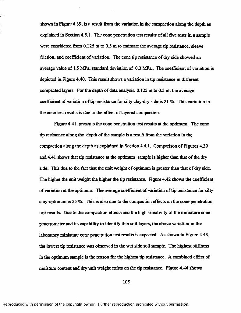
shown in Figure 4.39, is a result from the variation in the compaction along the depth as
explained in Section 4.5.1. The cone penetration test results o f all five tests in a sample
were considered from 0.125 m to 0.5 m to estimate the average tip resistance, sleeve
friction, and coefficient of variation. The cone tip resistance of dry side showed an
average value of 1.5 MPa, standard deviation of 0.3 MPa,. The coefficient o f variation is
depicted in Figure 4.40. This result shows a variation in tip resistance in different
compacted layers. For the depth of data analysis, 0.125 m to 0.5 m, the average
coefficient of variation of tip resistance for silty clay-dry side is 21 %. This variation in
the cone test results is due to the effect o f layered compaction.
Figure 4.41 presents the cone penetration test results at the optimum. The cone
tip resistance along the depth of the sample is a result from the variation in the
compaction along the depth as explained in Section 4.4.1. Comparison of Figures 4.39
and 4.41 shows that tip resistance at the optimum sample is higher than that o f the dry
side. This due to the fact that the unit weight of optimum is greater than that o f dry side.
The higher the unit weight the higher the tip resistance. Figure 4.42 shows the coefficient
of variation at the optimum. The average coefficient of variation of tip resistance for silty
clay-optimum is 25 %. This is also due to the compaction effects on the cone penetration
test results. Due to the compaction effects and the high sensitivity o f the miniature cone
penetrometer and its capability to identify thin soil layers, the above variation in the
laboratory miniature cone penetration test results is expected. As shown in Figure 4.43,
the lowest tip resistance was observed in the wet side soil sample. The highest stiffness
in the optimum sample is the reason for the highest tip resistance. A combined effect of
moisture content and dry unit weight exists on the tip resistance. Figure 4.44 shows
105
Reproduced with permission of the copyright owner. Further reproduction prohibited without permission.

Depth
(m
)
0.0
0.2
0.4
0.6
0.80 10 20 30 40 SO 60 70
COV of qc (%)0 10 20
COV of fs (%)
Figure 4.40 Coefficient of variation of laboratory cone penetration o f silty clay at dryside
106
Reproduced with permission of the copyright owner. Further reproduction prohibited without permission.

Depth
(m
)
Silty clay-optimum
0 1 2 3 4
Tip resistance, qc(MPa)
0.00 0.06 0.12 0.18
Sleeve friction, fs (MPa)
- M CPTl- MCPT2- MCPT3 •• MCPT4- MCPT5
Figure 4.41 Laboratory cone penetration of silty clay at optimum
107
Reproduced with permission of the copyright owner. Further reproduction prohibited without permission.

Depth
(m
)
0.0
0.2
0.4
0.6
0.80 10 20 30 40 50 60 70
COV of qc(%)10 20
COV of fs (%)30
Figure 4.42 Coefficient o f variation of laboratory cone penetration o f silty clay atoptimum
108
Reproduced with permission of the copyright owner. Further reproduction prohibited without permission.

Depth
(m
)
o.o
o.i
0.3
0.4
0.5
0.6
0.7
0.80 I 2
Tip resistance, qc(MPa)
Silty clay wet side
0.00 0.05 0.10
Sleeve friction, fs (MPa)
CenterMCPT2MCPT3MCPT4MCPT5
Figure 4.43 Laboratory cone penetration of silty clay at wet side
109
Reproduced with permission of the copyright owner. Further reproduction prohibited without permission.

Dept
h, m
0.0
0.2
0.4
0.6
0.8100500
COV of qc COV of fs
Figure 4.44 Coefficient of variation of laboratory cone penetration of silty clay at wetside
110
Reproduced with permission of the copyright owner. Further reproduction prohibited without permission.

the coefficient o f variation at the wet side. For the depth o f data analysis, 0.125 m to 0.5
m, average coefficient of variation of dp resistance for silty clay-wet side is 11.6 %.
Figure 4.45 shows the cone penetration test results at the dry side o f the heavy
clay. The average tip resistance of heavy clay- dry side is 1.3 MPa. The average tip
resistance of heavy clay- dry side is less than that of silty clay-dry side. This is due to
the soft nature o f heavy clay. As shown in Figure 4.46, for the range of data analysis,
coefficient of variation of tip resistance for heavy clay dry side, optimum, and wet side
are 13 %, 15 %, and 23 % respectively.
Figure 4.47 shows the cone penetration test results at the optimum of the heavy
clay. The average tip resistance o f heavy clay- optimum is 1.6 MPa. The average tip
resistance of heavy clay-optimum is also less than that of silty clay-optimum.
Coefficient of variation of tip resistance for heavy clay-optimum is 15 %.
Figure 4.48 present the cone penetration test results at the wet side o f the heavy
clay. The tip resistance at optimum sample is higher than that o f the dry side and wet
side samples because the highest stiffness is occurred at the optimum. The lowest tip
resistance was observed in the wet side soil sample due to the highest moisture content
Cone test result for silt is depicted in Figure 4.49 shows that tip resistance varies
with the depth. The highest tip resistance was observed in the optimum sample. The
lowest tip resistance was recorded in the wet side sample. For the range of data analysis,
coefficient of variation of tip resistance for silt dry side, optimum, and wet side are 15 %,
9 %, and 7 % respectively. Coefficient o f variation o f water content for silt dry side,
optimum, and wet side are 4.0 %, 3.0 %, and 22. %.
I l l
Reproduced with permission of the copyright owner. Further reproduction prohibited without permission.
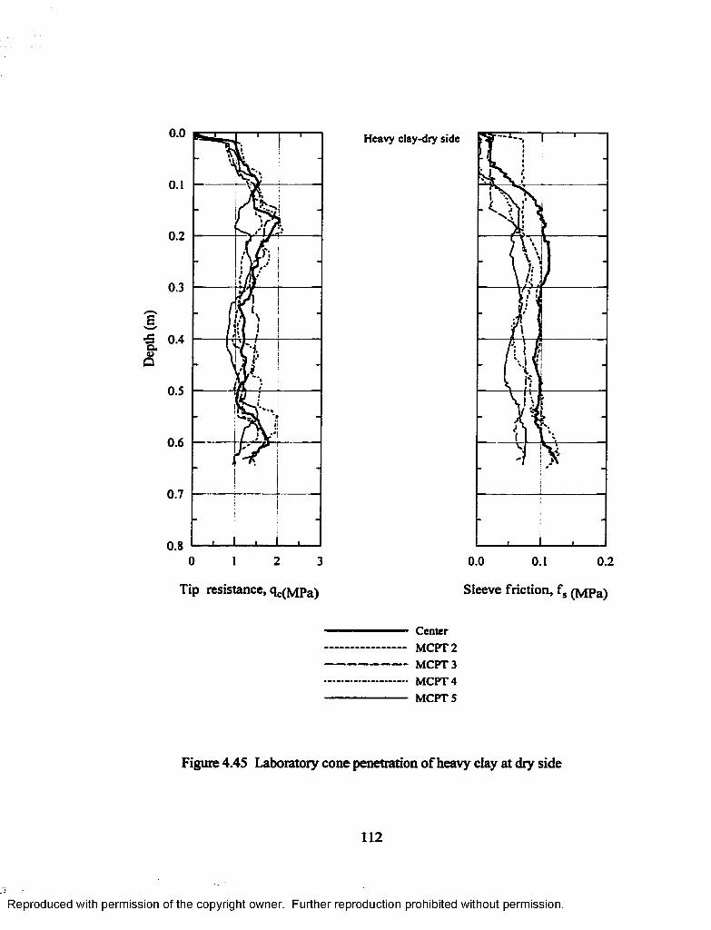
Depth
(m
)0.0
o.l
0.2
0.3
0.4
0.5
0.6
0.7
0.8
Heavy clay-dry side
0 1 2 3 0.0 0.1 0.2
Tip resistance, qc(MPa) Sleeve friction, fs (MPa)
— Cent er--------------------- MCPT2------------------------MCPT3---------------------- MCPT4---------------------- MCPT5
Figure 4.45 Laboratory cone penetration of heavy clay at dry side
Reproduced with permission of the copyright owner. Further reproduction prohibited without permission.

Dept
h, m
0.0
0.2
0.4
0.6
0.8100500
COV of qc0 50 100 150 200
COV of fs
Figure 4.46 Coefficient of variation of laboratory cone penetration o f heavy clay at dryside
113
Reproduced with permission of the copyright owner. Further reproduction prohibited without permission.

Depth
(m
)
0.0
0.1
0.2
0.3
0.4
0.5
0.6
0.7
0.80 1 2 3 0.0 0.1 0.2
Heavy clay-optimum
Tip resistance, qc(MPa) Sleeve friction, fs (MPa)1 Center
--------------------- MCPT2----------------------MCPT3---------------------- MCPT4---------------------- MCPT5
Figure 4.47 Laboratory cone penetration of heavy clay at optimum
114
Reproduced with permission of the copyright owner. Further reproduction prohibited without permission.

Depth
(m
)
0.0
0.2
0.3
0.4
0.5
0.6
0.7
0.80.0 0.5 1.0
Tip resistance, qc(MPa)
Heavy clay-wet side
0.00 0.06 0.12
Sleeve friction, fs (Mpa)
CenterM CPT2M CPT3M C PT4M CPT5
Figure 4.48 Laboratory cone penetration of heavy clay at wet side
115
Reproduced with permission of the copyright owner. Further reproduction prohibited without permission.

Depth
(m
)
Dry side Optimum0.0
0.1
0.2
0.3
0.4
0.5
0.6
0.70 2 4 6 8 10 0 2 4 6 8 10
Tip resistance, q ^ P a ) TiP resistance, qc(Mpa)
Wet side
»i ii !
; ;
5!
! Ii
!i
|
Uu
! f ti i I
i !1 ii i _t—iL-
0 2 4 6 8 10
Tip resistance, q ^ P a )
- M CPTl- MCPT2- M CPT3- MCPT4- MCPT5
Figure 4.49 Laboratory cone penetration of silt
116
Reproduced with permission of the copyright owner. Further reproduction prohibited without permission.

Cone test result for sand is depicted in Figure 4.50. The tip resistance of sand
varies with the depth due to the effect o f the layered compaction. For the range o f data
analysis, coefficient of variation o f tip resistance for sand dry side, optimum, and wet side
are 16 %, 9 %, and 11 % respectively.
4.5.4 Resilient Modulus
Figure 4.51 shows the resilient modulus test results for silty clay at dry side. A
high resilient modulus for a subgrade soil is desirable to obtain a resistance to
deformation due to traffic loading. As expected, the resilient modulus of silty clay
decreases as deviator
stress increases. The resilient modulus of silty clay is higher than that of heavy clay. The
cone tip resistance follows the same pattern. This is due to the higher stiffness in silty
clay and soft nature in heavy clay. At optimum (Figure 4.52) the highest resilient
modulus is observed. The highest soil stiffness at optimum may be a reason for this high
resilient modulus. The resilient modulus o f silty clay dry side is greater than that of wet
side (Figures 4.51 and 4.53). This due to the high water content in the wet side.
Figures 4.54,4.55, and 4.56 present the resilient modulus of heavy clay dry side,
optimum, and wet side respectively. At optimum (Figure 4.55) the highest resilient
modulus is observed. The resilient modulus of heavy clay dry side is greater than that of
wet side (Figures 4.54 and 4.56). Figure 4.57 shows the resilient modulus test results for
silt at dry side. As expected, the resilient modulus values of silt increases with bulk
stresses. The resilient modulus at wet side is lower than that at dry side. A higher water
content and lower stiffness result in lower resilient modulus. The highest resilient
modulus occurs at optimum. This is due to the highest stiffness at optimum.
117
Reproduced with permission of the copyright owner. Further reproduction prohibited without permission.

Depth
(m
)0.0
o.l
0.2
0.3
0.4
0.5
0.6
0.7
Sand-dry side Sand-optimumI- 1 ■ •• 1 - T '
IV llVS V•11*1' ■ 1' im il% i'.ftit Dli »l|*
!i
'.U ! Im i
Ii
i.ii••il i
§!(1 i
. 1i
Il i i ! ! ; i ; ! !
j l M M
n1
1 i |ii
___i___ 1 1 Ii 1 i10 15 20 5 10 15 20
Sand-wet side
i i ! r r ^
T- r
! I
Tip resistance, qg(MPa) TiP resistance, qc(Mpa)
0 5 10 15 20
Tip resistance, q^MPa)
- MCPT1- MCPT2- MCPT3 - MCPT4
- MCPT5
Figure 4.50 Laboratory cone penetration o f sand
118
Reproduced with permission of the copyright owner. Further reproduction prohibited without permission.

CQ&*S'w '
w£IBJ33•ooEavtnf£
100Silty clay-dry side .
Confining stressct. =41.3 kPaCTr =20.7 kPa
or. =0.0 kPa10
10010Deviator stress, cy,, (kPa)
Figure 4.51 Resilient modulus of silty clay at dry side
119
Reproduced with permission of the copyright owner. Further reproduction prohibited without permission.

100Silty ciay-optimum -
Pm
Confining stressa - =41.3 kPa
C/3
ct =20.7 kPa
a . =0.0 kPa
10010Deviator stress, a d (kPa)
Figure 4.52 Resilient modulus of silty clay at optimum
120
Reproduced with permission of the copyright owner. Further reproduction prohibited without permission.

100Silty clay-wet side ‘
Confining stressa_ =41.3 kPaCfl
ar =0.0 kPa
10010Deviator stress, <rd (kPa)
Figure 4.53 Resilient modulus of silty clay at wet side
121
Reproduced with permission of the copyright owner. Further reproduction prohibited without permission.

C3CL,
2inJ33■ooScuinc2
100
Confining stressa . =41.3 kPa
crc =20.7 kPa
<se =0.0 kPaHeavy clay dry side
10100101
Deviator stress, a d (kPa)
Figure 4.54 Resilient modulus of heavy clay at dry side
122
Reproduced with permission of the copyright owner. Further reproduction prohibited without permission.
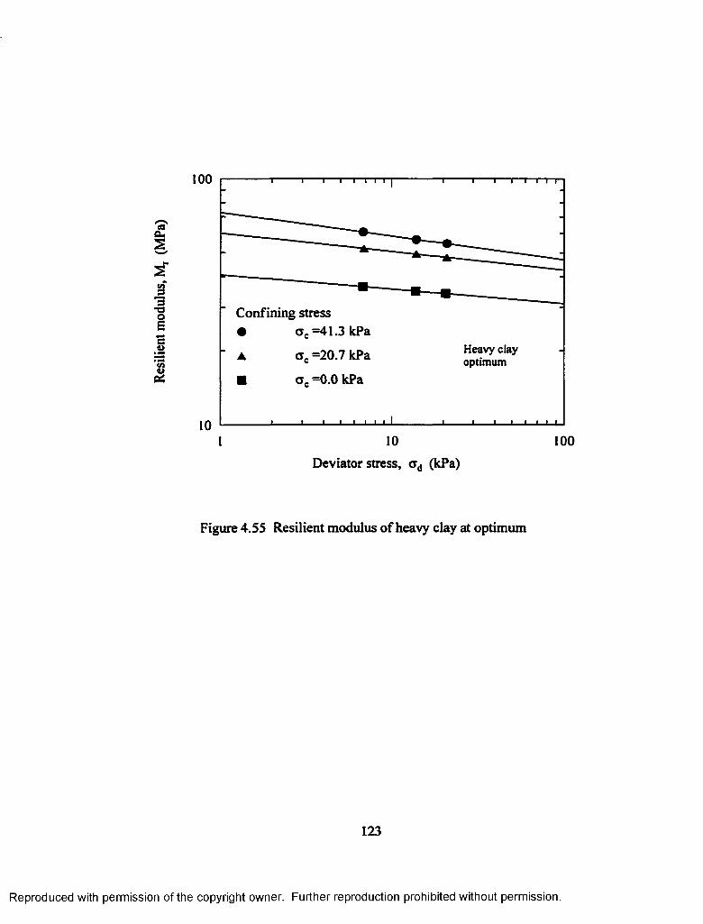
COft*S
s•ooSc4)
CD
c2
100
Confining stressa . =41.3 kPa
Heavy clay optimum=20.7 kPa
ct. =0.0 kPa
1010 100
Deviator stress, crd (kPa)
Figure 4.55 Resilient modulus of heavy clay at optimum
123
Reproduced with permission of the copyright owner. Further reproduction prohibited without permission.

100Confining stress
=41.3 kPa
=20.7 kPa
=0.0 kPa
3s•aoEc<ue/i&
Wet side
10010
Deviator stress, crd (kPa)
Figure 4.56 Resilient modulus of heavy clay at wet side
124
Reproduced with permission of the copyright owner. Further reproduction prohibited without permission.

1000Silt-dry side I
Oi
100
Confining stressct, =20.7 kPa crc =103.4 kPa
ctc =34.5 kPa oc =137.8 kPaa c =68.9 kPa
100 1000Bulk stress, a b (kPa)
Figure 4.57 Resilient modulus of silt at dry side
125
Reproduced with permission of the copyright owner. Further reproduction prohibited without permission.

Figure 4.58 presents the resilient modulus test results for sand at dry side. As
expected, the resilient modulus o f sand also increases with bulk stresses. The resilient
modulus at wet side is lower than that at dry side due to the higher moisture content and
lower stiffness at wet side. The highest resilient modulus occurs at optimum due to the
highest stiffness at optimum.
4.5.5 Effect of Moisture Content and Unit Weight
After the cone penetration test, the soil sample was subjected to the moisture
content and unit weight tests in different depths. For fine-grained soils and silt, unit
weight was estimated by using the sand cone test (LADOTD TR 401-95). Along the
depth of the soil sample, moisture contents were also obtained.
Moisture content, determined along the depth of soil sample of silty clay-dry side,
showed an average value of 14.2 %, standard deviation of 0.3 %, and coefficient of
variation of 1.8 % against the designed moisture content of 14.4 %. Coefficient of
variation of moisture content for silty clay dry side, optimum, and wet side are 1.8 %,
1.7 %, and 1.5 %, respectively. Coefficient of variation of water content for heavy clay
dry side, optimum, and wet side are 4.4 %, 2.2 %, and 1.3 % respectively. Coefficient of
variation of water content for sand dry side, optimum, and wet side are 1.6 %, 3.7 %, and
5.8 %.
Dry unit weight determined along the soil sample depth of silty clay-dry side
showed an average value o f 15.9 kN/m3, standard deviation of 0.2 kN/m3, and coefficient
of variation o f 1.2 % against the designed unit weight 16.1 kN/m3. Coefficient of
variation of dry unit weight for silty clay dry side, optimum, and wet side are 1.2 %,
2.0 %, and 1.2 %, respectively. Coefficient of variation of dry unit weight for heavy clay
126
Reproduced with permission of the copyright owner. Further reproduction prohibited without permission.

1000
cscus
sCO
3•oo£ •—* e vCO
(2
100
10
;— | , r - I —i---- 1— i—i—i—;Sand-dry side -
- 4 1 — !----------
- -P- -- Confining stress -
• oc =20.7 kPa ❖ ctc =103.4 kPaA crc =34.5 kPa + ctc =137.8 kPa
_■ a c =68.9 kPa
_1____________ i i____ i___ * » l 1 L100 1000
Bulk stress, a b (kPa)
Figure 4.58 Resilient modulus of sand at dry side
127
Reproduced with permission of the copyright owner. Further reproduction prohibited without permission.

dry side, optimum, and wet side are 5.0 %, 2.8 %, and 2.8 % respectively. Coefficient of
variation of dry unit weight for silt dry side, optimum, and wet side are
2.4 %, 7.6 %, and 3.8 %. Coefficient of variation of dry unit weight for sand dry side,
optimum, and wet side are 3.0 %, 6.2 %, and 2.2 %. This type of variation can be
expected due to the layered compaction effects. Among the four soil types, the maximum
coefficient of variation for tip resistance, water content, and dry unit weight are 25 %, 6
%, and 5 %, respectively.
Figures 4.59 and 4.60 depict the variation in the resilient modulus with the
moisture content In the wet side, as the moisture content increases effective deviator
stress decreases and hence the resilient modulus decreases. In the wet side, soil fabric is
dispersed whereas, in the dry side, soil is flocculated. Strength of the dispersed soil is
less than that o f flocculated soil. The resilient modulus is related to the strength o f soil.
In silty clay, the change in the resilient modulus in dry and wet sides was about 14 MPa
for the change in moisture content of about 7 %. In heavy clay, the change in the resilient
modulus in dry and wet sides was about 15 MPa for the change in moisture content of
about 10 %. This may result in the change in the overlay thickness of a pavement
significantly as explained in Section 4.6. Figures 4.61 and 4.62 indicate that as the unit
weight increases the resilient modulus increases. But it decreases with the increasing
moisture content Figures 4.63 and 4.64 show the same behavior for the tip resistance.
Therefore, the maximum resilient modulus and tip resistance occurred at the optimum.
4.5.6 Summary of the Laboratory Cone Testing
The laboratory cone test results were used to validate the proposed models,
developed in the field testing program. The predicted and measured resilient modulus
128
Reproduced with permission of the copyright owner. Further reproduction prohibited without permission.

«GCUs
cn S’3 • aoEeu
‘35c2
55.0
50.0
45.0
40.0
35.0
30.0
25.0
— — !— I— !— —i j'O ntim nm
1 ii 1
j^■1 ! i
Dry sjide 1r '! I1 <
J 1 1 upnm u m
i «T\1 !
u i y imc i! i \
i l l ! i !i :! ; !I i ^ ret side m I ! I :1 |i i 1 ' ■
i i 1
1 1| Wet side!1 i 1 i
0.0 10.0 20.0w(%)
30.0 40.0
Heavy clay Silty clay
Figure 4.59 Variation in the resilient modulus with moisture content of fine-grained soil
129
Reproduced with permission of the copyright owner. Further reproduction prohibited without permission.

££S '33T3OE€u
60Qptimi
Dry side50
40 Optimum j
30Dr^ sidi
20
rWct side10
00.0 5.0 10.0 15.0 20.0 25.0
w (%)
▲ Silt+ Sand
Figure 4.60 Variation in the resilient modulus with moisture content of coarse-grainedsoil
130
Reproduced with permission of the copyright owner. Further reproduction prohibited without permission.

60'3'
2e/fJ33"OIs<u
40
200.5 1.0 1.50.0
Heavy clay Silty clay
yd (kN/m3)/ w (%)
Figure 4.61 Variation of the moisture content, unit weight, and resilient modulus forfine-grained soil
/■“N 60«*ft.s 502r/s 40J3 30•ooe 203.2 10'eft4>ft£ 0
! ! ! ! ! ! !, ■" r ■ t . _ - r : ■ - r1 (! 1' / ! I T * ! .
i
If !. . . . X J i i
----- 1------!---- -
-! T " T ' ...— — i—
—
- U!!
------1------
i 1 1
'i
+★
SiltSand
Yd (kN/m3 ) / w (%)
Figure 4.62 Variation of the moisture content, unit weight, and resilient modulus forcoarse-grained soil
131
Reproduced with permission of the copyright owner. Further reproduction prohibited without permission.

C3CL2CT*«O
e/3
2o.E—
2
0
Heavy clay Silty clay
0.0 0.5 1.0 1.5
Yd (kN/m3 ) / w (%)
Figure 4.63 Variation of the moisture content, unit weight, and tip resistancefor fine-grained soil
COCL2
u
C/3
£&
8
6
4
2
0
+★
SiltSand
0 1 2 3 4
Yd (kN/m3 ) / w (%)
Figure 4.64 Variation of the moisture content, unit weight, and tip resistancefor coarse-grained soil
132
Reproduced with permission of the copyright owner. Further reproduction prohibited without permission.

values are presented in Figures 4.65 and 4.66. Most o f the data fall close to the line of
equality. The measured and predicted modulus values are not significantly different.
Tables 4.9 and 4.10 present the result of the laboratory cone test.
Tables 4.5 and 4.11 present the elastic properties. The modulus of elasticity (E)
were estimated from the laboratory repeated load triaxial testing. The Poisson’s ratio (v)
was assumed.
4.5.7 Traffic Stress Analysis
The traffic stress models, given in equations (4.3) and (4.4), were applied to
predict the resilient modulus of fine-grained soil using the laboratory cone test results.
The predictions are presented in Figures 4.67 and 4.68. Most of the data fall close to the
line o f equality. The measured and predicted modulus values are not significantly
different. The results of the stress analysis are presented in Table 4.10.
4.5.8 Preliminary Design Charts
From the laboratory resilient modulus and cone penetration test results,
preliminary charts were developed to evaluate the resilient modulus from the cone
penetration test parameters. But they were not verified due to lack o f data. According to
the type of soil, different resilient modulus and cone tip resistance can be obtained. The
resilient modulus, moisture content, dry unit weight, and the cone tip resistance charts
were prepared. Knowing the cone tip resistance, resilient modulus can be estimated from
these charts. This may be useful in pavement designs as an estimation of the resilient
modulus. Figures 4.69 to 4.76 present the simplified design charts for heavy clay, silty
clay, silt, and sand respectively. As illustrated in Figure 4.69, when the soil type and the
cone tip resistance are known, a chart for that soil type can be used for evaluating
133
Reproduced with permission of the copyright owner. Further reproduction prohibited without permission.

90 80
« 70 eu2 60 S 501 40=3i 30 S 20
10
00 10 20 30 40 50 60 70 80 90
Predicted M,. (MPa)
Figure 4.65 In-situ resilient modulus from the laboratory cone test for fine-grained soil
Controlled tests
Silty clay —
* Heavy clay _
134
Reproduced with permission of the copyright owner. Further reproduction prohibited without permission.

C3CU2
2•oa33U2
908070605040 Controlled tests
3020
[ 1 Sand
10
00 10 20 30 40 50 60 70 80 90
Predicted Mr (MPa)
Figure 4.66 In-situ resilient modulus from the laboratory cone test for coarse-grained soil
135
Reproduced with permission of the copyright owner. Further reproduction prohibited without permission.

Table 4.9 Summary of the laboratory cone test results
Depth(m)
qc(MPa)
fs(MPa) (kPa) (kPa)
w(%)
Yd(kN/m3)
Siltyclay
dry 0.31 1.5 0.0763 3.58 5.72 14.4 16.1opt. 0.31 1.8 0.0816 3.82 6.11 18.0 16.7wet 0.31 1.1 0.0705 3.80 6.08 21.8 16.1
Heavyclay
dry 0.31 1.3 0.0758 3.93 5.19 26.4 13.1opt. 0.31 1.6 0.1060 4.20 5.54 31.4 13.6wet 031 0.4 0.0965 4.09 5.40 36.4 12.8
Siltdry 0.31 3 2 0.1622 3.03 5.72 10.7 16.4opt. 0.31 5.7 0.0032 3.28 6.17 15.2 17.2wet 0.31 0.9 0.0010 3.15 5.93 20.4 15.9
Sanddry 0.31 2.9 0.0010 2.79 5.25 5.0 16.1opt. 0.31 7.6 0.0087 2.92 5.50 8.1 16.4wet 0.31 1.0 0.0300 2.86 5.39 11.0 15.7
Legend: Mr- resilient modulus, cre- confining (minor principal) stress,<tv- vertical (major principal) stress, / , - sleeve friction, w- water content, yj- dry unit weight, yw- unit weight of water, and q c- cone resistance.
Reproduced with permission of the copyright owner. Further reproduction prohibited without permission.

Table 4.10 Stress analysis for the laboratory cone tests
Soil type Depth(m)
Controlled test-insitu Controlled test-insitu & traffic
<se(kPa)
crd(kPa)
Mr(MPa)
<*c(kPa) (kPa)
Mr(MPa)
Siltyclay
dry 0.31 3.58 2.14 46.20 7.88 11.30 39.36opt. 0.31 3.82 2.29 48.30 8.12 11.50 48.84wet 0.31 3.80 2.28 32.33 8.10 11.50 29.93
Heavyclay
dry 0.31 3.93 1.26 42.09 9.31 7.27 44.06opt. 0.31 4.20 1.34 43.20 9.62 7.37 42.67wet 0.31 4.09 1.31 26.63 9.43 7.43 25.08
Siltdry 0.31 3.03 2.69 23.94 6.88 10.70 35.28opt. 0.31 3.28 2.89 35.18 7.15 10.90 40.21wet 0.31 3.15 2.78 13.85 7.04 10.80 18.00
Sanddry 0.31 2.79 2.46 48.52 6.58 12.10 53.92opt. 0.31 2.92 2.58 52.35 6.63 12.10 57.84wet 0.31 2.86 2.53 17.27 6.49 12.00 23.31
Legend: a c - Confining stress, a d - Deviator stress, M, - Resilient modulus
Reproduced with permission of the copyright owner. Further reproduction prohibited without permission.

Table 4.11 Elastic properties of the soil
Elastic Property PRF-Silt Sand
E (MPa) 27.1 45.9
V 0.35 0.35
Legend: E- Elastic modulus, v- Possion’s ratio
138
Reproduced with permission of the copyright owner. Further reproduction prohibited without permission.

C8CUsw
s•o1u2
60
50
40
30
20
10
06010 20 30 40 500
Predicted Mr (MPa)
▲ Controlled test-silty clay# Controlled test-heavy clay
Figure 4.67 Prediction o f resilient modulus from the traffic stress modelfor fine-grained soil
139
Reproduced with permission of the copyright owner. Further reproduction prohibited without permission.

40
Controlled-trafficcoarse-grained
0 10 20 30 40 50 60 70 80 90Predicted Mr (MPa)
▲ Controlled test-silt# Controlled test-sand
Figure 4.68 Prediction of resilient modulus from the traffic stress modelfor coarse-grained soil
Reproduced with permission of the copyright owner. Further reproduction prohibited without permission.

Silty clay
★ Resilient Modulus
# Tip resistance
6.0
| Optimum5.0
Dry 46.2
Wet Estimated resilient modulus 32.3 j
<uu 3.0Wet side |
Optimum
Measured -tip resistance.
Wet1.0
0.01.0 1.50.5
60
50
40
30
20
10
yd (kN/m3 ) / w (%)
Figure 4.69 A chart for estimating in-situ resilient modulus of silty clay from conepenetration
141
Reproduced with permission of the copyright owner. Further reproduction prohibited without permission.
Resil
ient
mod
ulus
, M,
(M
Pa)

Tip
resis
tance
, q,
(MPa
)
Heavy clay
★ Resilient Modulus# Tip resistance
5.0
D rytimi
4.0 Estimated resilienl modulus
3.0
Wet-
Wet side2.0
Measured tip resistance1.0 Dry-
Wet
0.00.4 0.5 0.60.3
50
40
30
20
10
Yd (kN/m ) / w (%)
Figure 4.70 A chart for estimating in-situ resilient modulus of heavy clay from conepenetration
142
Reproduced with permission of the copyright owner. Further reproduction prohibited without permission.
Resil
ient
mod
ulus
, M,
(MPa
)

# Tip resistance
★ Resilient Modulus
6.0I Optimujn
5.0
404.0cuOptimum
vcr3.0
Dry2.0
Wet side Dry sideWet
1.0Wei
0.00.5 1.0 1.5 2.0
Yd (lcN/m3 ) / w (%)
Figure 4.71 A chart for estimating in-situ resilient modulus of silt from cone penetration
143
Reproduced with permission of the copyright owner. Further reproduction prohibited without permission.
Resil
ient
mod
ulus
, M,
(M
Pa)

# Tip resistance
★ Resilient Modulus
808.0I Optimum J l
707.0
606.0Optimum
cu5.0
Dry!
a»u 404.0
303.0 Dry)o. Dry sWet side
202.0Wet
1.0Wet
0.01.0 2.0 3.0 4.0
yd (kN/m3) / w (%)
Figure 4.72 A chart for estimating in-situ resilient modulus of sand from cone penetration
144
Reproduced with permission of the copyright owner. Further reproduction prohibited without permission.
Resil
ient
mod
ulus
, M,
(M
Pa)
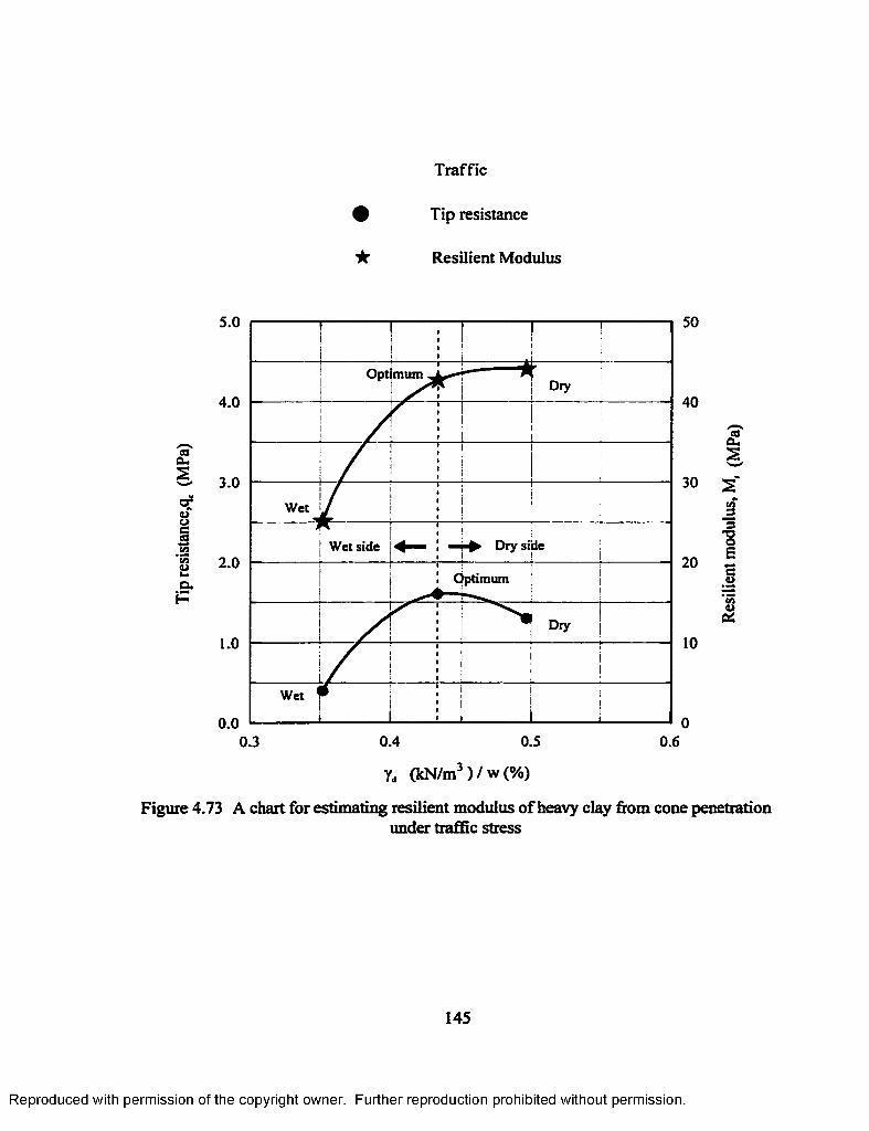
Traffic
# Tip resistance
★ Resilient Modulus
5.0
OptimumDry
4.0
"o'cuw 3.0
Wet
Dry sideWet sideC/1
2.0Qptimumo.
pDry
1.0
Wet
0.00.3 0.4 0.5
Yd (kN/m3 ) / w (%)
50
40
30
20
10
0.6
Figure 4.73 A chart for estimating resilient modulus of heavy clay from cone penetrationunder traffic stress
145
Reproduced with permission of the copyright owner. Further reproduction prohibited without permission.
Resil
ient
mod
ulus
, M,
(M
Pa)
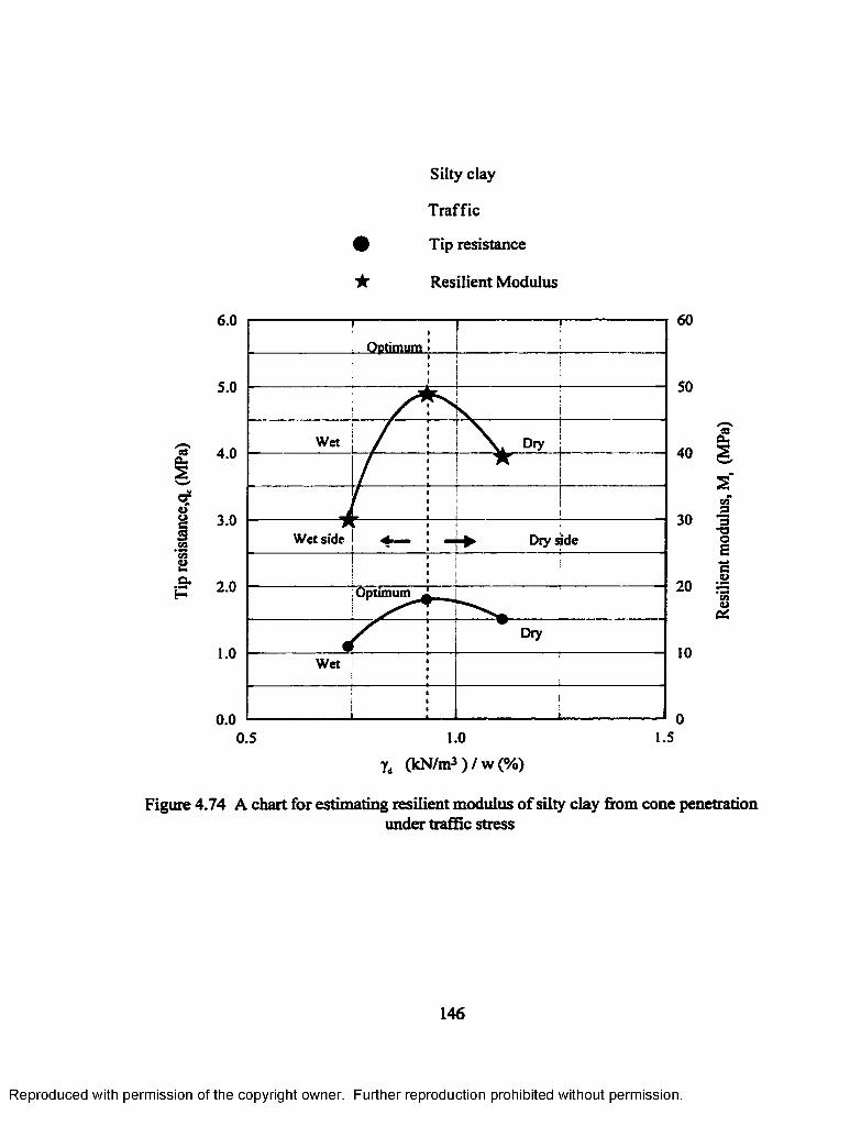
Silty clay
Traffic
Tip resistance
Resilient Modulus
0.5 1.0
6.0
{ Optimum
5.0
Wet1?c- 4.0sd?i f§ 3.0
Wet side
2cuP 2.0 I Optimum
1.0Wet
0.0
yd (kN/m3 ) / w (%)
60
50
40
30
20
10
1.5
Figure 4.74 A chart for estimating resilient modulus of silty clay from cone penetrationunder traffic stress
146
Reproduced with permission of the copyright owner. Further reproduction prohibited without permission.
Resil
ient
mod
ulus
, M
, (M
Pa)

Traffic
# Tip resistance
★ Resilient Modulus
6.0Optin um
5.0
Optimum<2 4.02 Dry
Dry3.0
Wetjside Dry side
So .P 2.0
Wet
0.00.5 1.0 1.5 2.0
yd (kN/m3 ) / w (%)
Figure 4.75 A chart for estimating resilient modulus of silt from cone penetration undertraffic stress
147
Reproduced with permission of the copyright owner. Further reproduction prohibited without permission.
Resil
ient
mod
ulus
, M
, (M
Pa)

Traffic
# Tip resistance
★ Resilient Modulus
COCUSwd*u
2Q.H
8.0Optimum
7.0
Optimum6.0
Dry5.0
4.0
Wet side i D ry side i3.0
Dry
Wet2.0
1.0Wet
0.02.0 3.01.0 4.0
80
70
60
50
40
30
20
10
0
yd (kN/m3 ) / w (%)
Figure 4.76 A chart for estimating resilient modulus of sand from cone penetration undertraffic stress
148
Reproduced with permission of the copyright owner. Further reproduction prohibited without permission.
Resil
ient
mod
ulus
, M
, (M
Pa)

the resilient modulus. In the absence of the moisture content and dry unit weight, these
charts can still be used. But in this case, an approximate moisture content is to be
guessed in order to assign the data point in the dry, optimum, or wet side in the moisture-
unit weight curve. Otherwise, except at optimum, it is recommended that an average
value of two resilient moduli be considered, corresponding to the dry and wet side. When
the soil type is uncertain or unknown, a visual inspection or other engineering judgement
is required to be classified as heavy clay, silty clay, silt, or sand.
How to use the chart (refer to Figures 4.69 to 4.76):
(1) Select the corresponding tip resistance from the field cone penetration test.
(2) To determine dry side or wet side, read the corresponding dry unit weight (kN/m3)
to moisture content (%) ratio from the chart of corresponding soil type.
(3) Read the corresponding resilient modulus from the chart
(4) If the moisture content or dry unit weight is unknown, read the two resilient
modulus values, except at the optimum, corresponding to the dry and wet side.
Then take the average as the required value. This will provide a reasonable guess
for the resilient modulus.
4.5.8.1 A Chart for Estimating Effective Subgrade Soil Resilient Modulus Using the Serviceability Criteria
The AASHTO guide for design of pavement structures (1993) stipulates analysis
the subgrade soil for different moisture seasons in a year, such as dry and rainy, to
estimate an effective resilient modulus for design purpose. Covering the primary
moisture seasons, such as dry and rainy, the resilient modulus tests (AASHTO T- 294)
should be performed on roadbed soil samples. By knowing the seasonal resilient moduli
149
Reproduced with permission of the copyright owner. Further reproduction prohibited without permission.

of roadbed soil, the relative damage (Ur) of the pavement can be estimated. From the
relative damage, an effective resilient modulus value for flexible pavements can be
obtained by using the design charts and equations provided by the AASHTO guide for
design of pavement structures. The same design charts were used while being modified
the estimation of the resilient modulus from the cone penetration test results. This
procedure consists of performing several cone penetration tests in different moisture
seasons in a year, estimating corresponding moisture content, unit weight o f soil, and soil
stresses. Seasonal resilient modulus for each month can be evaluated by using a
correlation or charts proposed in this study. The relative damage can be estimated by the
equation (4.5), given in the AASHTO guide for design of pavement structures (1993).
The effective design resilient modulus can be estimated from the average relative damage
and the AASHTO equation. The effective roadbed resilient modulus, corresponding to
the average relative damage, can be estimated.
Steps in this procedure:
1. As shown Figure 4.77, divide a year into one-month or one-half month seasons. All
the seasons (time periods in the chart) in a year must be equal.
2. Allocate the seasonal tip resistance, sleeve friction, moisture content, dry unit weight,
confining stress, and deviator stress in their respective time slots.
3. Compute the seasonal roadbed resilient modulus by using a correlation or charts
proposed in this study.
4. Estimate the relative damage by using the charts or equations given in the AASHTO
guide for design o f pavement structures (1993).
5. Add the all relative damage values and compute an average relative damage value.
150
Reproduced with permission of the copyright owner. Further reproduction prohibited without permission.

Month qc
(MPa)
fs
(MPa)
w
(%)
Yd
(kN/m3)
<*c
(kPa)
<*d
(kPa)
Mr
(psi)
u r
Jan.
Feb.
March
April
May
June
July
August
Sept.
Oct.
Nov.
Dec.
Total 2 U r
Legend: Ur-relative damage, n • number o f months, M,- resilient modulus (psi)
Figure 4.77 A chart for estimating effective roadbed soil resilient modulus using theserviceability criteria
Reproduced with permission of the copyright owner. Further reproduction prohibited without permission.

6 . Estimate an effective resilient modulus, corresponding to the average relative damage,
by using the charts or equations given in the AASHTO guide for design of pavement
structures (1993).
In the case of rigid pavements, an effective modulus of subgrade reaction (k-
value) must be calculated from the seasonal roadbed soil resilient modulus with the aid of
the charts or equations given in the AASHTO guide for design of pavement structures.
Average relative damage U r = --------- (4.5)n
The AASHTO equation for relative damage,
Ur = U 8 x lO * xM ;232 (4.6)
4.5.8.2 An Example for Using the Proposed Charts
The summary of the data for silty clay, used to characterize the subgrade soil
resilient modulus, is presented in Table 4.12. A year is divided into 24 half-month
seasons. The wet seasons are from mid-January to May and mid-September to mid-
December. The dry seasons are from June to mid-September and mid-December to mid-
January.
Table 4.12 Cone penetration and soil test data for silty clay
Test parameter qc f, w Yd(MPa) (MPa) (%) (lcN/m3) (kPa) (kPa)
dry season 1.5 0.0763 14.4 16.1 3.58 2.14wet season 1.1 0.0705 21.8 16.1 3.80 2.28
Legend: M r- resilient modulus, erc- confining (minor principal) stress,erv- vertical (major principal) stress, / , - sleeve friction, w~ water content, y<r dry unit weight, j v unit weight o f water, and q c~ tip resistance
152
Reproduced with permission of the copyright owner. Further reproduction prohibited without permission.

The resilient modulus values are estimated from the chart given in Figure 4.69 for
silty clay for in-situ condition. The resilient modulus values are 46.2 MPa (670S psi) and
32.3 MPa (4688 psi) for dry and wet seasons respectively.
From Figure 4.78, Average relative damage = 6.798 =0.28
Effective subgrade soil resilient modulus = 5200 (psi) = 35.8 (MPa)
4.6 Sensitivity of the AASHTO Flexible Pavement Design Equation
The effect o f change in the subgrade soil resilient modulus on the AASHTO
flexible pavement design equation is analyzed. The AASHTO design equation:
where,
W,s- predicted number of 18-kip equivalent single axle load (ES AL),
ZR - standard deviation, SN- structural number,
R- reliability,
Sa- combined standard error of the traffic prediction and performance prediction,
Mr- effective resilient modulus of subgrade soil, and
APSI- difference between the initial design serviceability index and the design terminal
serviceability index.
The AASHTO design equation is iteratively evaluated for a typical pavement
section, as shown in Figure 4.79, by varying the value of the overlay thickness while
24
log l0 wx% = ZRSa + 9361ogl0(S tf + l ) -
0 2 0 4 10Q4 l°8io 8.07(4.7)
{after AASHTO, 1993)
153
Reproduced with permission of the copyright owner. Further reproduction prohibited without permission.

Month qe
(MPa) (MPa)
w
(%)
Yd
(kN/m3)
<*c
(kPa) (kPa)
Mr
(psi)
u r
Jan. 1.5 0.0763 14.4 16.1 3.58 2.14 6705 0.1571.1 0.0705 21.8 16.1 3.80 2.28 4688 0.359
Feb. 1.1 0.0705 21.8 16.1 3.80 2.28 4688 0.3591.1 0.0705 21.8 16.1 3.80 2.28 4688 0.359
March 1.1 0.0705 21.8 16.1 3.80 2.28 4688 0.359l.l 0.0705 21.8 16.1 3.80 2.28 4688 0.359
April l.l 0.0705 21.8 16.1 3.80 2.28 4688 0.3591.1 0.0705 21.8 16.1 3.80 2.28 4688 0.359
May 1.1 0.0705 21.8 16.1 3.80 2.28 4688 0.3591.1 0.0705 21.8 16.1 3.80 2.28 4688 0.359
June 1.5 0.0763 14.4 16.1 3.58 2.14 6705 0.1571.5 0.0763 14.4 16.1 3.58 2.14 6705 0.157
July 1.5 0.0763 14.4 16.1 3.58 2.14 6705 0.1571.5 0.0763 14.4 16.1 3.58 2.14 6705 0.157
Aug. 1.5 0.0763 14.4 16.1 3.58 2.14 6705 0.1571.5 0.0763 14.4 16.1 3.58 2.14 6705 0.157
Sept 1.5 0.0763 14.4 16.1 3.58 2.14 6705 0.1571.1 0.0705 21.8 16.1 3.80 2.28 4688 0.359
Oct 1.1 0.0705 21.8 16.1 3.80 2.28 4688 0.3591.1 0.0705 21.8 16.1 3.80 2.28 4688 0.359
Nov. 1.1 0.0705 21.8 16.1 3.80 2.28 4688 0359
1.1 0.0705 21.8 16.1 3.80 2.28 4688 0.359
Dec. l.l 0.0705 21.8 16.1 3.80 2.28 4688 0.3591.5 0.0763 14.4 16.1 3.58 2.14 6705 0.157
Total 6.798
Figure 4.78 Estimation of the effective resilient modulus from the cone test parameters
154
Reproduced with permission of the copyright owner. Further reproduction prohibited without permission.

keeping the design ESAL constant. The design variables are as follows. W,8= 5,000,000
ESALs, 1?= 95 %, S = 0.35, APSI= 1.9, and design M= 34.5 MPa. This results in S N =
5. Layer coefficients are assumed as a,= 0.42, af= 0.16 and a}=0.10 for the surface
course, base, and subbase respectively. The effect of variation in the resilient modulus on
the overlay thickness is presented in Figure 4.80. According to Figure 4.80, variation in
the resilient modulus may have a significant effect on the overlay thickness. Therefore
selecting a correct design resilient modulus is desired in pavement design.
Surface102 mm (4.0"), asphalt concrete, at = 0.42
Base241 mm (9.5"), a2 = 0.16
Subbase 457 mm (18.0"), a3 = 0.10
Figure 4.79 A typical pavement section
155
Reproduced with permission of the copyright owner. Further reproduction prohibited without permission.

Incr
emen
tal o
verla
y th
ickne
ss (
mm
)
150
100
-20Change in resilient modulus, Mr (MPa)
-50
-100
-150
Figure 4.80 Variation in the overlay thickness with the resilient modulus
156
Reproduced with permission of the copyright owner. Further reproduction prohibited without permission.

CHAPTER 5
FIELD APPLICATION OF THE PROPOSED MODELS
After development and verification of the proposed models, a successful attempt
has been made to apply them in road rehabilitation projects in Louisiana with the support
of Louisiana Department of Transportation and Development
Resilient modulus is an input parameter for evaluating the structural number (SN)
in flexible pavement designs. The CPT can also be used in a rehabilitation project of an
existing pavement for evaluating the resilient modulus of subgrade soil. In this case, for
the required traffic, reliability, initial serviceability, and terminal serviceability, a new
structural number, based on the resilient modulus, can be estimated. By knowing the
existing structural number, the difference in the structural numbers can be determined.
Then required overlay thickness can be estimated.
For example, the developed correlations were applied in the road rehabilitation
projects at Louisiana State Route LA-482, LA-513, and Henderson levee road. Several
undisturbed soil samples were retrieved from the subgrade of these rehabilitation sites.
These samples were tested for resilient modulus (AASHTO T- 294) and other soil
properties in the laboratory according to the procedures described previously. The
proposed correlations were also used to predict the resilient modulus. Then the measured
and predicted resilient modulus were compared. Figures 5.1,5.2, and 5.3 present the
cone penetration test results o f the LA-482, LA-513, and Henderson levee road
respectively. Figures 5.4,5.5, and 5.6 show the resilient modulus test results of the LA-
482 , LA-513, and Henderson levee road respectively. Figures 5.7 and 5.8 compare the
measured and predicted resilient modulus under in-situ and traffic loading conditions
157
Reproduced with permission of the copyright owner. Further reproduction prohibited without permission.

Depth
(m
)
0.0
1.0
2.00 10 20 0.0 1.0 2.0
Tip resistance, qc(MPa) Sleeve friction, fs (MPa)
a
0 25 50 75 100
Friction ratio, Rf (%)
LA-482BH3BH4
Figure 5.1 Cone penetration test results of the LA-482
158
Reproduced with permission of the copyright owner. Further reproduction prohibited without permission.

0.0
1.0
2.010 200
Tip resistance, qc(MPa)
0.0
1.0
2.00.60.0 0.3
Sleeve friction, fs (MPa)
LA-513
Figure 5.2 Cone penetration test results o f the LA-513
159
Reproduced with permission of the copyright owner. Further reproduction prohibited without permission.

•5S'Q
0.0
1.0
2.0
3.0
0 1 2 3 4 5 6 7
Tip resistance, qc(MPa)
0.0
2.0
3.0
0.2 0.30.0 0.1
Sleeve friction, fs (MPa)
Henderson-0.1
Figure 5.3 Cone penetration test results of the Henderson levee road
160
Reproduced with permission of the copyright owner. Further reproduction prohibited without permission.

C3a*s
in33•oiIMaS
1000BH3- depth=0.8 m
Confining stress
ctc =20.7 kPa
<j- =0.0 kPa100
1010 100
Deviator stress, crd (kPa)
100
BH4Sample depth=0.8 m
Confining stress
a . =20.7 kPa
a . =0.0 kPa
10010Deviator stress, a d (kPa)
Figure 5.4 Resilient modulus test results of the LA-482
161
Reproduced with permission of the copyright owner. Further reproduction prohibited without permission.
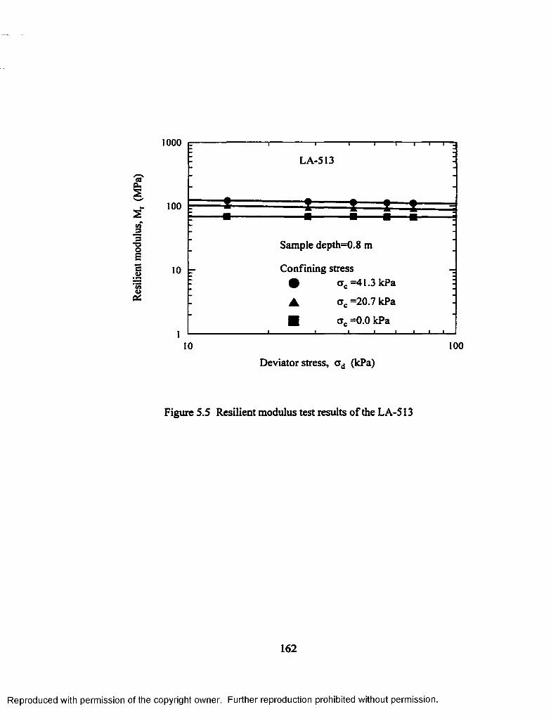
1000 P-
LA-513
100 t I
3T3OSe<un<2
10 -
Sample depth=0.8 m
Confining stresscrc =41.3 kPa
oc =20.7 kPa
crc =0.0 kPa I_______ I I_____l_
10 100
Deviator stress, <rd (kPa)
Figure 5.5 Resilient modulus test results of the LA-513
162
Reproduced with permission of the copyright owner. Further reproduction prohibited without permission.

Resil
ient
mod
ulus
, Mr
(MPa
)100
Henderson-0.1
Sample depth=0.8 m
Confining stress
a . =0.0 kPa
10010Deviator stress, a d (kPa)
Figure 5.6 Resilient modulus test results of the Henderson levee road
163
Reproduced with permission of the copyright owner. Further reproduction prohibited without permission.

' 1 ' ' 'lU M ' 1 ' 1 ' 'LA482-BH4 /LA-513 /Henderson-O. \ f
0 10 20 30 40 SO 60 70 80 90 100 Predicted Mr (MPa)
Figure S.7 Prediction of resilient modulus under in-situ condition
Reproduced with permission of the copyright owner. Further reproduction prohibited without permission.

C8CUs
T 3293<U
1009080706050403020100
i i i i i j iLA482-BH3
i 1 i 1 i y/ i-A LA482-BH4
r+ LA-513 f “
- 0 Henderson 0 .1 ./ —
—❖ /
-
'A \ . 1 . 1 . 1 , 1 , ! ,Traffic -
1 , I , 1 , ‘
0 10 20 30 40 50 60 70 80 90 100 Predicted M,. (MPa)
Figure 5.8 Prediction of resilient modulus under traffic loading
165
Reproduced with permission of the copyright owner. Further reproduction prohibited without permission.

respectively. Most o f the data fall close to the line of equality. The measured and
predicted modulus values are not significantly different. Therefore, the proposed models
are successful in predicting the resilient modulus in the rehabilitation projects. Tables 5.1
and 5.2 present the summary of test results.
Table 5.1 Summary of the test results
BoreholeDepth
(m)qc (MPa) fj(MPa)
Water
content(%)
Dry unit
weight (kN/m3)LA-513 0.8 5.21 0.3163 21.3 16.9
Henderson 0.1 0.8 1.62 0.0718 23.3 15.4LA-482-BH3 0.8 3.31 0.1349 17.0 18.6LA-482-BH4 0.8 3.39 0.0686 18.0 17.9
Table 5.2 Summary of the stress analysis
\ Depth
(m)
In-situ In-situ + traffic
CTc
(kPa) (kPa)
Measured
Mr (MPa)
Predicted
M,. (MPa)
CTc
(kPa) (kPa)
Measured
Mr (MPa)
Predicted
Mr (MPa)LA-
5130.8 11.6 4.8 88.9 92.6 16.4 10.8 93.5 99.6
Hen. 0.8 10.7 4.4 46.0 42.0 15.5 9.8 45.4 35.0BH3 0.8 12.3 5.1 62.9 68.4 15.9 11.9 64.1 62.4BH4 0.8 12.0 4.9 59.9 60.7 15.6 11.7 55.9 51.1
Legend: Mr- resilient modulus (MPa), ctc- confining (kPa), deviator stress (kPa),
f s l e e v e friction (MPa), w (% )- water content, Yd- <hy unit weight (kN/m3), yw- unit weight o f water
(kN/m3), q c-cone resistance(MPa), BH- borehole, and Hen- Henderson 0.1.
166
Reproduced with permission of the copyright owner. Further reproduction prohibited without permission.

CHAPTER 6
SUMMARY AND CONCLUSIONS
This dissertation presented a study to assess the applicability of the intrusion
technology for evaluating the resilient modulus of subgrade soil in pavements. The field
and laboratory testing programs were performed at seven soil sites (eight soils), in
Louisiana, to develop correlations between the resilient modulus and cone penetration
parameters. The cone penetration tests were performed with the 2 cm2 and IS cm2
miniature cones at the selected sites. The CPT tests were performed with a IS cm2 (44
mm in diameter) cone to verify the CIMCPT data. Undisturbed and disturbed soil
samples were also retrieved from the field. Resilient modulus values were determined at
the laboratory according to the AASHTO T-294 test method. The cone penetration and
resilient modulus tests were performed at the same in-situ conditions to simulate the same
field variation. In addition to the cone penetration and resilient modulus tests, several
other soil tests, such as triaxial, hydrometer, soil classification, unit weight, standard
proctor, specific gravity, Atterberg limit, and moisture content, were also performed.
These tests were used to classify soil and determine strength parameters. The test results
were analyzed and critically evaluated. Comparison of the test results showed that
CIMCPT results follow the same patterns as those of the CPT.
Four statistical models, to predict the resilient modulus from the cone test
parameters, were developed for fine-grained and coarse-grained soil with in-situ and
traffic stress conditions. These models correlate the resilient modulus to the cone
penetration parameters, resilient modulus, moisture content, dry unit weight, and stress
levels. Both in-situ stresses and traffic stresses were considered. These models were
167
Reproduced with permission of the copyright owner. Further reproduction prohibited without permission.

calibrated using the field test results of two soil types and used to predict the resilient
modulus o f different soil types. All o f the models produced a high coefficient of multiple
determination, 0.99. These models can be used to predict the resilient modulus of
subgrade soil from the cone penetration test data. The parameters, such as confining
stress, deviator stress, moisture content, dry unit weight, and the cone tip resistance, have
a significant effect on the models between resilient modulus and cone penetration data.
Since these models incorporate these parameters, they can be used to estimate the
resilient modulus at any moisture-unit weight combination. This satisfies a requirement
in the AASHTO pavement design procedure which stipulates to evaluate an effective
subgrade resilient modulus by taking into account the subgrade moisture content variation
throughout the year.
The laboratory cone penetration, resilient modulus, and soil property tests were
also performed on the laboratory compacted soil samples to investigate the effects of the
variation in the moisture content and unit weight on the resilient modulus as well as to
validate the four models, developed in the field testing program. Also, from the
laboratory cone penetration test data and resilient modulus test results, preliminary design
charts were developed to evaluate the resilient modulus from the cone parameters. A
designer can utilize these charts to estimate an effective subgrade soil resilient modulus.
A successful application of the proposed models in predicting the resilient modulus at the
rehabilitation projects was performed. In this case, the predicted and measured resilient
modulus values were not significantly different These results supported the validity o f
the proposed models in predicting resilient modulus of subgrade soil by the soil
parameters and cone penetration test results. Therefore, the developed models in
168
Reproduced with permission of the copyright owner. Further reproduction prohibited without permission.

predicting the resilient modulus o f subgrade soil were successful. Major findings of this
investigation are summarized below.
(1) Applicability of the cone penetration test to evaluate the resilient modulus of
subgrade soil was demonstrated. Four models to predict the resilient modulus
from the cone penetration parameters, two for fine-grained and two for coarse
grained soils with in-situ and traffic stress conditions, were developed. The
coefficient o f multiple determination was as high as 0.99 for all the models. The
RMSE values were very low. These values indicate the high predictive capability
of these models. These models were validated with the field and laboratory cone
test results. The predicted and measured resilient modulus values from these
models were not significantly different. The field applications o f the models, in
the road rehabilitation projects, were performed.
(2) Simplified design charts were developed to estimate an effective subgrade soil
resilient modulus. Due to the lack of data, they were not verified.
(3) The higher the tip resistance, the higher the resilient modulus of subgrade soil.
(4) The parameters such as the cone tip resistance, confining stress, deviator stress,
moisture content, and dry unit weight have a significant effect on the models
between resilient modulus and cone penetration data. The resilient modulus
increases with the unit weight and it decreases with the moisture content. There is
a combined effect from the moisture content and unit weight on the resilient
modulus of soil. The resilient modulus increases with the confining pressure.
The resilient modulus increases with the bulk stress for coarse-grained soils. The
resilient modulus decreases with the deviator stress for cohesive soils.
169
Reproduced with permission of the copyright owner. Further reproduction prohibited without permission.

(5) The CIMCPT results are repeatable and reliable. The CIMCPT system is
successful in shallow depth investigation in cohesive soils. The miniature cone
penetrometer records a higher tip resistance and lower sleeve friction than the
reference cone does. Coarse-grained soil exhibits higher tip resistance and lower
sleeve friction than fine-grained soil does. In other words, fine-grained soil
exhibits lower tip resistance and higher sleeve friction than coarse-grained soil
does. The reference cone and miniature cone test results show the similar pattern
along the depth while the magnitude is slightly different.
6.1 Future Recommendation
Implementation of the proposed models in the actual road designs and
rehabilitation projects is important. Expanding the proposed design charts for more soil
types is recommended. Future research should be aimed at developing a large data base
that would be used for prediction of the resilient modulus of subgrade soil from the cone
penetration test parameters.
170
Reproduced with permission of the copyright owner. Further reproduction prohibited without permission.

REFERENCES
AASHTO Interim guide for Design o f Pavement Structures, American Association of State Highway and Transportation Officials, 1986.
AASHTO T 294-921, American Association of State Highway and Transportation Officials,"Resilient modulus of Unbound Base/Subbase Materials and Subgrade Soils- SHRP Protocol P46, AASHTO, T-294-92I, 1992, pp. 52-65.
AASHTO T 294-94, American Association of State Highway and Transportation Officials, "Resilient Modulus of Unbound Granular Base/Subbase Materials and Subgrade Soils-SHRP Protocol P46, AASHTO, T 294-94,1995, pp. 794-807.
ASTM, American Society for Testing and Materials Annual book o f ASTM Standards, Volume 4.03, Road and Paving Materials; Paving Management Technologies, 1993.
ASTM, American Society for Testing and Materials Annual book of ASTM Standards, Volume 14.02, 1990.
Alavilli, P., V., M., "Investigation of the use of resilient modulus for Louisiana soils in design of pavements," Master Thesis, Civil Engineering Dept., Louisiana State University, Baton Rouge, 1995.
Allen, A., J., "Development of a correlation between physical and fundamental properties o f Louisiana soils," Master's Thesis, Dept of Civil Engineering, LSU, 1996.
Allen, D., L., "Mr Testing in Kentucky," Workshop on Resilient Modulus Testing, Oregon State University, Corvallis, 1989.
Barksdale, R., D., Rix, G., J., Itani, S., Khosla, P., N., Kim, R., Lambe, C., and Rahman, M., S., "Laboratory Determination o f Resilient Modulus for Flexible Pavement Design," Interim Report No. 1-28, NCHRP, TRB, Geogia Institute o f Technology, 1990.
Campanella, R.G., and Robertson, P.K., "Applied Cone Research," Symposium on Cone Penetration Testing and Experience, Geotechnical Engineering Division, ASCE, 1981, pp. 343-362.
Campanella, R., G ., Gillespie, D., and Robertson, P.,K., "Pore Pressures During Cone Penetration ", Proc., 2nd European Symposium on Penetration Testing, Amsterdam, Vol. 2, 1982, pp. 507-512.
Campanella, R., G ., Robertson, P.JC., and Gillespie, D., "Cone penetration testing in deltaic soils," Canadian Geotechnical Journal, Vol. 20,1983, pp. 23-35.
171
Reproduced with permission of the copyright owner. Further reproduction prohibited without permission.

Carmichael IE, R., F., and Stuart, E., "Predicting Resilient Modulus: A study to determine the mechanical properties of subgrade soils," TRB, No. 1043,1986.
Chen, B. S., and Mayne, P. W ., “Profiling the Over consolidation Ratio o f Clay by Piezocone Tests,” Report GIT-CEEGEO-94-1. Georgia Tech Research Corporation and Georgia Institute of Technology, School of Civil & Environmental Engineering, 1994.
Clark, J.I., and Meyerhof, G.G., "The Behavior of Piles Driven in Clay. I. An Investigation of Soil Stress and Pore Water Pressure as Related to Soil Properties," Canadian Geotechnical Journal, Vol. 9,1972, pp. 351-373.
Das, B.M., “Advanced Soil Mechanics,” Hemisphere publishing corporation, 1983, pp.406.
De Lima, D.C. and Tumay, M.T., “Scale Effects in Cone Penetration Tests,” Special Publication No. 27, Proc. Geotechnical Engineering Congress, ASCE, Boulder, CO, 1991, pp. 38-51.
Drumm, E., C., Reeves, J., S., Madgett, M., R., and Trolinger, W., D., "Subgrade Resilient Modulus Correction for Saturation Effects," Journal of Geotechnical and Geoenvironmental Engineering, Vol. 123, No.7, July 1997, pp. 663-670.
ELSYM5, Developed by SRA Technologies, Inc., Under contract to Federal Highway Administration, October, 1985.
Fredlund, D., G., Bergan, A., T., and Wong, P., K., "Relation Between Resilient Modulus and Stress Conditions for Cohesive Subgrade Soils", Transportation Research Record, No. 642, 1977, pp. 73-81.
Holden, J.C., "Laboratory Research on Static Cone Penetrometrs," Internal Report CE- SM-71-1, Dept. O f Civil Engineering, University of Florida, 1971.
Kamal, M., A., et al., "Field and Laboratory Evaluation o f the mechanical Behavior of Unbound Granular Materials in Pavements," Transportation Research Record, No. 1406, 1993, pp. 88-97.
Kim, D.,S., Stokoe, K., H., II, "Characterization of Resilient Modulus o f Compacted Subgrade Soils Using Resonant Column and Torsional Shear Tests, Transportation Research Record, No. 1369, 1992, pp. 83-81.
Konard, J.M. and Roy, M., "Bearing Capacity o f Friction Piles in Marine Clay," Geotechnique, Vol. 37, No. 2,1987, pp.163-175.
Kurup, P.U., "Calibration Chamber Studies of Miniature Piezocone Penetration Tests in Cohesive Soil Specimens", PhT). Dissertation, Louisiana State University, 1990.
172
Reproduced with permission of the copyright owner. Further reproduction prohibited without permission.

Kurup, P.U. and Tumay, M.T., "Continuous Intrusion Miniature Cone Penetration Test System for Transportation Applications," Seventh International Conference on Low- Volume Roads, TRB, No. 1652, Vol. 1, Baton Rouge, Louisiana, 1999, pp. 228-235.
Lee, K.W., Marcus, A.S. and Mao, H., "Determination of Effective Soil Resilient Modulus and Estimation of Layer Coefficients for Unbound Layers of Flexible Pavement in Rhode Island," Report No. URI-CVET-94-l Res Rept No. 1,1994 Sept. 30.
McGee, N., "Cold Region Facility- Subgrade Soils," Workshop on Resilient Modulus Testing, Oregon State University, Corvallis, 1989.
Mohammad, L.N., Huang, B., Puppala, A., and Alen, A., "A Regression Model for Resilient Modulus of Subgrade Soils," 78th Annual Meeting of the Transportion Research Board, Washington D.C., 1999.
Mohammad, L.N., Alavilli, P., Puppala, A.J., "Data Acquisition System for Determining the Resilient Modulus o f Soils," ASCE Geotechnical special publication 37: Advances in Site Characterization: Data Acquisition, Management and Interpretation, 1993, Dallas,pp. 27-41.
Mohammad, L. N., Puppala, A. J., and Alavilli, P., "Influence of Testing Procedure and LVDT Location on Resilient Modulus of Soils", Transportation Research Record, No. 1462, 1994, pp. 91-101.
Mohammad, L. N., Puppala, A., and Alavilli, P., "Effect of Strain Measurements on Resilient Modulus of Granular Soils," Dynamic Geotechnical Testing: Second Volume, ASTM STP 1213, ASTM, 1994, pp.202-221.
Mohammad, L. N. and Puppala, A., "Resilient Properties of Laboratory Compacted Subgrade Soils," National Academy of Science, Transportation Research Record, No. 1504,1995, pp. 87-102.
M ohammad, L.N., Titi, H.H., and Herath Ananda, "Evaluation of Resilient Modulus of Subgrade Soil by Cone Penetration Test Results," Seventh International Conference on Low-Volume Roads, Transportation Research Records, No. 1652, Vol. 1, Baton Rouge, Louisiana, May 1999, pp. 236 to 245.
Mohammad, L.N., Titi, H.H., and Herath Ananda, "Intrusion Technology: An Innovative Approach to Evaluate Resilient Modulus o f Subgrade Soil," Application o f Geotechnical Principles in Pavement Engineering, ASCE, Geotechnical Special Publication Number 85, Geo Congress’98, Boston, Massachusetts, 1998, pp. 39-58.
M ohammad, L.N., Titi, H.H., and Herath Ananda, "Investigation of the Applicability of Intrusion Technology to Estimate the Resilient Modulus of Subgrade Soil," Final Report, Louisiana Transportation and Research Center project No. 98-6GT, April 2000.
173
Reproduced with permission of the copyright owner. Further reproduction prohibited without permission.

Monismith, C., L., "M, testing- Interpretation of Laboratory Results for Design Purposes/' Workshop on Resilient Modulus Testing, Oregon State University, Corvallis, 1989.
Nataatmadja, A. and Parkin, A., "Characterization of Granular Materials for Pavements," Canadian Geotechnical Journal, Vol.26, No.4, 1989, pp. 725-730.
Nazarian, S. and Feliberti, M., "Methodology for Resilient Modulus Testing of Cohesionless Subgrades," Transportation Research Record, No. 1406,1993, pp. 108-115.
Parkin, A.K. and Lune, T., 1982, "Boundary Effects in the Laboratory Calibration o f a Cone Penetrometer for Sand," Proceedings o f the European Symposium on Penetration testing, Vol.2, Amsterdam, pp. 761-768.
Pezo, R. and Hudson, W .R.," Prediction Models o f Resilient Modulus for Nongranular Materials", Geotechnical Testing Journal, Vol.17, N o.3,1994, pp.349-355.
Puppala, A.J., Acar, Y.B., and Tumay, M.T., "Cone Penetration in Very Weakly Cemented Sands," ASCE, Journal of Geotechnical Engineering, Vol 121, No. 8, 1995, pp.589-600.
Puppala, A., Mohammad, L.N., Allen, Aaron, "Engineering Behavior of Lime Treated Subgrade Soils,” National Academy of Science, Transportation Research Record, No. 1546, Issues in Geotechnical Engineering Research, 1996, pp. 24-31.
Puppala, A., Mohammad, L.N., Allen, A., "Rutting Potential o f Subgrade Soils from Repeated Load Triaxial Resilient Modulus Test," ASCE Journal of Materials in Civil Engineering, Vol. 11, No. 4,1999, pp. 274-282.
Rada, G. and Witczak, M., W .," Comprehensive Evaluation of Laboratory Resilient Moduli Results for Granular Material," Transportation Research Record, No. 810,1981, pp. 23-33.
Robertson, P.,K., and Campanella, R., G., "Interpretation of Cone Penetration Tests- Part I: Sand," Canadian Geotechnical Journal, Vol.20, N o.4,1983, pp. 724-733.
Robertson, P.,K., and Campanella, R., G., "Interpretation of Cone Penetration Tests- Part H: Clay," Canadian Geotechnical Journal, Vol.20, N o.4,1983, pp. 734-745.
Schmertmann, J.H., "Guidelines for Cone Penetration Test: Performance and Design", Report No. FHWA-TS-78-209, FHWA, Washington, D.C., 1978, pp. 145.
Sebaaly, P.E., Tabatabaee, N. and Scullion, T., “Comparison of Backcalculated Moduli from Falling Weight Deflectometer and Truck Loading,” TRB No. 1377, 1992, pp. 88- 98.
174
Reproduced with permission of the copyright owner. Further reproduction prohibited without permission.

Strategic Highway Research Program, “Resilient Modulus of Unbound Granular Base, Subbase Materials and Subgrade Soils,” SHRP Protocol P-46, UG07, SS07,1989.
Titi, H.H., Mohammad, L.N., and Tumay, M.T., “Miniature Cone Penetration Tests in Soft and Stiff Clays,” Geotechnical Testing Journal, ASTM, Vol. 23, No.4, December 2000, pp.432-443.
Tumay, M., T., Boggess, R.L., and Acar, Y, “Subsurface Investigation with Piezocone penetrometer,” Proceedings, ASCE National Convention, S t Louis, 1981, pp. 325-342.
Tumay, M.T. and de Lima, D.C., “Calibration and Implementation of Miniature Electric Cone Penetrometr and Development, fabrication and Verification of the LSU In-situ Testing Calibration Chamber (LSU/CALCHAS),” LTRC/FHWA Report No. GE-92/08, 1992, pp. 240.
Tumay, M.T., and Kurupp, P.U., and Boggess, R.L., “A continuous intrusion electronic miniature cone penetration test system for site characterization,” Geotechnical Site Characterization, Proc. 1“ International Conf. On site characterization-ISC’98, Atlanta, Vol. 1, 1998, pp. 1183-1188.
Tumay, M.T., and Kurup, P.U .,, “Calibration and Implementation of Miniature Electric Cone Penetrometers for Road and Highway Design and Construction Control,” LTRC State Project No. 736-13-0036, 1997.
Tumay, M.T., “Implementation o f Louisiana Electric Cone Penetrometer System (LECOPS) for Design of Transportation Facilities, Executive Summary, FHWA/LA, Report No. LA-94/280 A&B, 1994.
Tumay, M., T., Acar, Y., B., "Piezocone Penetration Testing in Soft Cohesive Soils," Strength Testing of marine Sediments: Laboratory and In-Situ Measurements, ASTM, STP 883, ASTM, Philadelphia, PA, 1985, pp. 72-83.
Ullidtz, P., "Pavement Analysis," Elsevier Publications, New York, 1987.
Uzan, J., "Charaterization o f Granular Materials", Transportation Research Record, No. 1022, TRB, 1985, pp. 52-59.
Wissa, A., E., Martin, R.T., and Garlanger, J.E., "The Piezometer Probe", Proc., ASCE Conference on In-situ Measurement of Soil Properties, Raleigh, NC, Vol. 1,1975, pp. 536-545.
175
Reproduced with permission of the copyright owner. Further reproduction prohibited without permission.

APPENDIX A
RESILIENT MODULUS TEST RESULTS
176
Reproduced with permission of the copyright owner. Further reproduction prohibited without permission.

Table A. 1 Resilient modulus test results for silty clay at controlled test
(kPa) (kPa)M,
(Mpa) dry side
COV(%)
Mr(Mpa)
optimum
COV(%)
Mr (Mpa)
wet side
COV(%)
41 14 59.57 4.1 79.09 2.0 38.01 3.4
41 28 55.84 5.5 74.10 1.9 37.69 4.6
41 41 51.54 5.2 69.07 1.7 36.91 4.6
41 55 47.87 2.1 64.92 4.8 36.47 7.6
41 69 45.96 7.5 62.18 2.7 35.28 8.3
21 14 46.70 5.2 63.18 5.5 32.69 2.4
21 28 41.28 7.4 57.82 2.1 31.89 3.6
21 41 38.81 7.3 54.28 4.3 31.21 6.1
21 55 37.72 3.2 51.18 5.4 30.56 7.7
21 69 36.99 5.6 49.99 3.9 29.37 6.7
0 14 34.66 7.6 40.27 4.2 27.43 9.9
0 28 30.67 9.3 39.44 2.3 26.44 9.4
0 41 29.08 9.2 38.77 3.5 25.65 8.1
0 55 28.57 9.3 38.42 5.5 24.86 9.7
0 69 28.06 7.6 38.23 8.7 24.43 9.2
177
Reproduced with permission of the copyright owner. Further reproduction prohibited without permission.
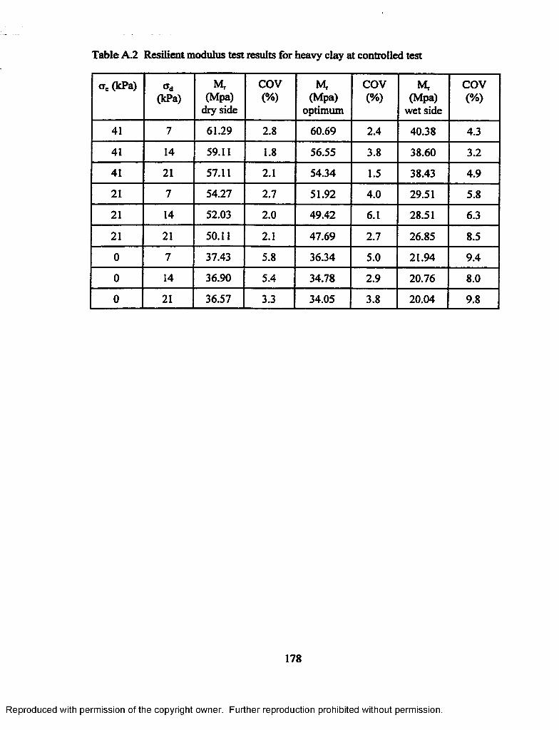
Table A.2 Resilient modulus test results for heavy clay at controlled test
<rc (kPa)(kPa)
M, (Mpa)
dry side
COV(%)
Mr(Mpa)
optimum
COV(%)
M, (Mpa)
wet side
COV(%)
41 7 61.29 2.8 60.69 2.4 40.38 4.3
41 14 59.11 1.8 56.55 3.8 38.60 3.2
41 21 57.11 2.1 54.34 1.5 38.43 4.9
21 7 54.27 2.7 51.92 4.0 29.51 5.8
21 14 52.03 2.0 49.42 6.1 28.51 6.3
21 21 50.11 2.1 47.69 2.7 26.85 8.5
0 7 37.43 5.8 36.34 5.0 21.94 9.4
0 14 36.90 5.4 34.78 2.9 20.76 8.0
0 21 36.57 3.3 34.05 3.8 20.04 9.8
178
Reproduced with permission of the copyright owner. Further reproduction prohibited without permission.

Table A 3 Resilient modulus test results for silt at controlled test
(kPa) (kPa)Mr
(Mpa) dry side
COV(%)
Mr(Mpa)
optimum
COV(%)
Mr (Mpa)
wet side
COV(%)
21 21 58.94 4.1 56.25 5.3 33.94 9.5
21 41 60.51 3.2 56.82 5.6 34.80 7.2
21 62 64.27 4.6 57.39 9.0 35.42 4.7
34 34 78.03 2.9 76.98 4.3 60.82 4.2
34 69 80.81 3.0 77.62 3.6 61.92 4.2
34 103 82.37 4.6 78.39 4.6 63.27 5.0
69 69 121.33 3.3 110.21 2.8 103.52 2.5
69 138 126.62 4.3 111.23 3.6 104.70 2.8
69 207 126.45 3.0 113.71 32 105.12 3.1
103 69 155.98 3.1 135.29 2.4 146.27 1.7
103 103 157.93 2.0 136.35 2.5 148.48 2.3
103 207 164.00 1.6 137.40 3.4 151.41 1.7
138 103 187.01 1.5 165.13 2.0 180.67 1.7
138 138 189.94 1.8 167.21 1.7 182.84 2.3
138 276 191.98 1.8 167.90 2.8 184.16 1.9
179
Reproduced with permission of the copyright owner. Further reproduction prohibited without permission.

Table A.4 Resilient modulus test results for sand at controlled test
<*c(kPa) (kPa)
Mr (Mpa)
dry side
COV(%)
M,(Mpa)
optimum
COV(%)
Mf(Mpa)
wet side
COV(%)
21 21 75.51 2.2 79.17 3.1 42.92 7.6
21 41 75.97 2.1 79.79 4.2 43.74 3.0
21 62 76.71 2.3 80.49 3.8 45.04 3.3
34 34 105.00 2.0 107.68 3.0 70.20 3.7
34 69 106.00 2.1 108.39 3.2 70.75 5.5
34 103 107.15 1.9 110.00 2.3 72.06 4.6
69 69 172.58 1.3 174.07 1.4 143.99 2.7
69 138 171.05 1.4 174.76 1.8 144.17 2.7
69 207 165.74 1.5 171.34 1.3 146.58 1.5
103 69 220.66 1.0 234.07 1.9 213.99 1.6
103 103 225.22 0.9 237.06 1.1 217.50 1.6
103 207 220.71 0.8 234.30 1.3 214.19 1.5
138 103 257.80 0.9 271.46 1.4 251.97 1.8
138 138 262.22 0.8 276.17 1.5 255.39 1.2
138 276 252.64 1.1 271.56 0.9 246.28 1.0
180
Reproduced with permission of the copyright owner. Further reproduction prohibited without permission.

APPENDIX B
PROCEDURE FOR MODEL DEVELOPMENT
181
Reproduced with permission of the copyright owner. Further reproduction prohibited without permission.

B.1 The Procedure for Model Development
The development o f the proposed model for fine-grained soils under in-situ
condition is described in this appendix. The data for the model development are given in
Tables 4.3 and 4.4 of Chapter 4. The results of silty clay and heavy clay were selected for
the fine-grained (in-situ) model development. The steps of the model development are
presented below.
Step 1: From Tables 4.3 and 4.4 of Chapter 4, input the variables, Mr- resilient modulus
(MPa), a c- confining (minor principal) stress (kPa), a d- deviator stress (kPa), c ry -
vertical stress (kPa), qc- tip resistance (MPa), f ,- sleeve friction (MPa), w- water
content (as a decimal), yd- dry unit weight (kN/m3), and yw- unit weight of
water (kN/m3).
Step 2: The variables were arranged according to the required physical conditions,
described in Section 4.4, Chapter 4, as in the nondimensional forms. Several
trials of regression analysis were performed with different ratio values o f the
resilient modulus to power terms of confining stress (M / ctc0 4S, M / ctc0-30, and
M / ctc° 5S). Among all these, the model with M / a c0'55 yielded the highest R2 and
the lowest RMSE value. By increasing the power term of the confining stress
above 0.55 creates impractical resilient modulus values in the model prediction.
Therefore, the power term for the confining stress was selected as 0.55.
Step 3: The model can parametrically be described as,
/
a.055 ac
C VV + A — (B.l)
182
Reproduced with permission of the copyright owner. Further reproduction prohibited without permission.

where, p„ p2, Pi are regression coefficients. As a first order approximation,
the dependent variable (M,/ ctc° 55) varies linearly with the independent variables.
A linear multiple regression analysis was performed by the Statistical Analysis
System (SAS) program (Table B .l). If the regression coefficients are positive in
the regression analysis, the physical conditions are satisfied. For example, if p 2 in
equation (B .l) is positive, as the moisture content increases the resilient modulus
decreases.
Step 4: Table B.2 shows the results of the regression analysis for fine-grained soil (in-
situ). Four models were developed, two for fine-grained and two for coarse
grained soil with in-situ and traffic stress conditions.
183
Reproduced with permission of the copyright owner. Further reproduction prohibited without permission.

Table B .l The SAS program for the model development
dm 'output;log;clear;’log; options ps=*60 ls=72 pageno=l; data one;infile 'd:\ananda\In-situ analysis\insitu-fine.dat’;input Mr qc f, w yd ac <yd;run;data two;input Mj. qc f, w yd oc <rd;Cctjrcis *. 2.1* 0.1042 0.21 16.9 8.6 7.8rdata three; set one two; gw=yd/9.81;<Tv=CTd+crc;fr=f,/av;cl=<rc**0.55;mc=Mr/ (cl) ;qv=»qc/ov;qg=*gw;fg=fr/w;keep qc qv Mr me f, fr qg fg w gd gw av <jd cl oc;proc reg data=«three;model mc=qv fg qg/clm cli noint;id m;run;quit;
184
Reproduced with permission of the copyright owner. Further reproduction prohibited without permission.

Table B.2 The results o f the regression analysis
Dependent Variable r MCAnalysis of Variance
Source DFSum of Squares
MeanSquare F Value
Model 3 1038.17090 346.05697 185.331Error 8 14.93788 1.86724U Total 11 1053.10878
Root MSE 1.36647 R-square 0.9858Dep Mean 8.82070 Adj R-sq o.9805C.V. 15.49160
Parameter EstimatesParameter Standard T for HO:
Variable DF Estimate Error Parameter=0QV 1 31.789744 23.18114903 1.371FG 1 74.807433 162.25682949 0.461QG 1 4.079008 0.73730501 5.532
Dep Var Predict Std Err Lower95%Obs M MC Value Predict Mean
1 48.4 12.1189 12.4691 0.723 10.80202 50.4 11.0837 12.8038 0.872 10.79263 54.1 13.5461 13.9794 1.200 11.21204 63.34 15.8597 13.7399 0.736 12.04265 60.74 13.3576 13.3514 0.672 11.80216 14.3 3.6558 4.9715 0.561 3.67787 14.6 3.3020 4.8562 0.584 3.51048 24.68 6.3095 5.2058 0.565 3.90299 26.2 5.9255 5.0916 0.542 3.841010 24.76 6.3299 5.3600 0.532 4.132311 24.49 5.5388 5.1217 0.577 3.791212 • • 13.3610 2.460 7.6882
Lower95% Upper95%Obs M Predict Predict Residual
1 48.4 8.9042 16.0341 -0.35022 50.4 9.0656 16.5421 -1.72013 54.1 9.7856 18.1732 -0.43324 63.34 10.1608 17.3190 2.11985 60.74 9.8401 16.8627 0.006246 14.3 1.5652 8.3778 -1.31577 14.6 1.4298 8.2827 -1.55428 24.68 1.7960 8.6156 1.10379 26.2 1.7015 8.4818 0.833910 24.76 1.9782 8.7418 0.969911 24.49 1.7012 8.5421 0.4172
Lower95% Opper95%Obs M Predict Predict Residual12 * 6.8718 19.8503
Sum of Residuals 0.077195Sum of Squared Residuals 14.9379Predicted Resid SS (Press) 31.6035
185
Prob>F0 . 0 0 0 1
Prob > ITI 0.2075 0.6570 0.0006
CJpper95%Mean
14.136314.815116.746815.437214.90076.26526 .2 0 2 16.50876.34236.58776.452119.0338
Reproduced with permission of the copyright owner. Further reproduction prohibited without permission.

VITA
Ananda Herath was bom in Sri Lanka. He received his bachelor o f science degree
in engineering (first class (honors) from the University of Peradeniya, Sri Lanka, in 1983
December. He worked for the University of Peradeniya as an instructor from 1984
January to 1984 August. He was a project engineer in the Mahaweli Engineering and
Construction Agency (MECA), Sri Lanka, from 1984 August to 1984 October. He also
worked for the University of Peradeniya as an assistant lecturer from 1984 November to
1986 September. He was a master’s student at the University of Tokyo from 1986
October to 1988 September. He received his master’s degree in civil engineering
(structural engineering) in 1988 September from the University of Tokyo. Then he was a
consulting engineer in Japan from 1988 October to 1995 September. He gained in
experience in design of bridges, pile foundations, culverts, retaining walls, and other
structural designs in Japan. He has been a doctoral student at the Louisiana State
University since 1996 January. He is also a Professional Engineer (P.E.) in Louisiana,
U.S.A. He will receive his doctoral degree in civil engineering (transportation
engineering) in August, 2001.
186
Reproduced with permission of the copyright owner. Further reproduction prohibited without permission.
DOCTORAL EXAMINATION AND DISSERTATION REPORT
candidates Ananada H.M.P.J. Hearth
Major Field: C iv i l Engineering
Title of Diaaertation: A Study o f the A p p l i c a b i l i t y o f Intrus ion Technology for Evaluating R e s i l i e n t Modulus o f Subgrade S o i l
Approved:
^Graduate Sc&ool
EXAMINING COM M ITTEE:
Date of Krami nation:
June 7 , 2001_________
Reproduced with permission of the copyright owner. Further reproduction prohibited without permission.