A Study of Micro-Scale Jet Pumps

by

Ole Mattis Nielsen

S.B. Electrical Engineering, M.I.T., June 2001

Submitted to the Department of Electrical Engineering and Computer Science

in Partial Fulfillment of the Requirements for the Degree of

Master of Engineering in Electrical Engineering and Computer Science

at the Massachusetts Institute of Technology

February 8, 2002 JUL 3 1 2002

LIBRARIE _

The author hereby grants to M.I.T. permission to reproduceand distribute publicly paper and electronic copies of this thesis

and to grant others the right to do so.

Author

Certified by

Certified by_

Accepted by

Department of Electrical Engineering and Computer ScienceFebruary 8, 2002

Martin A. SchmidtThesis Supervisor

Klavs F. Jensen

:Thesisjupervisor

Arthur C. SmithChairman, Department Committee on Graduate Theses

- -H

2

A Study of Micro-Scale Jet Pumps

by

Ole Mattis Nielsen

Submitted to the Department of Electrical Engineering and Computer Sciencein Partial Fulfillment of the Requirements for the Degree of

Master of Engineering in Electrical Engineering and Computer Scienceat the Massachusetts Institute of Technology

February 8, 2002

Abstract

A study of micro-scale jet pumps has been carried out and is presented in thisthesis. The work was motivated by the desire for an electrically passive fuel-air deliverysystem to a micro-generator that is currently being researched. Micron-size dimensionsare needed due to requirements for very low flow rates.

The concept of an ideal jet pump and the limits of jet pump performance areintroduced. Then the main problem of the micro-scale devices is approached: laminarflow profiles and increased viscous friction. A substantial deterioration of the aspirationperformance is seen with the scaling down of devices. The discussion is supported byanalytical solutions and finite volume simulations.

A set of first generation micro-scale jet pumps have been designed and micro-fabricated. While these devices fail to meet the micro-generator requirements foraspiration of air, some knowledge was accrued about geometry and operationoptimization.

Finally, a new concept for a better device exhibiting more ideal jet pump behavioris proposed and briefly studied. While this seems like a possibly promising road to take,the thesis limits itself to some suggestions on how to approach this concept in futurework.

Thesis Supervisor: Martin A. SchmidtTitle: Professor of Electrical Engineering

3

4

Table of Contents

Table of Contents .......................................................................................................... 5

Table of Figures .................................................................................................................. 7

A cknow ledgem ents ........................................................................................................ 9

N om enclature .................................................................................................................... 11

1. Introduction ................................................................................................................... 13

2. Background and physics of jet pum ps....................................................................... 15

2.1 The nozzle ........................................................................................................ 16

2.2 The throat ........................................................................................................ 17

2.3 The suction cham ber ........................................................................................ 19

2.4 Thesis study...................................................................................................... 19

3. The ideal jet pum p.................................................................................................... 21

3.1 A tm ospheric outlet pressure............................................................................ 21

3.2 N on-atm ospheric outlet pressure.................................................................... 23

3.3 The ideal jet pum p approxim ation ...................................................................... 26

4. N on-ideal jet pum ps discussed and sim ulated........................................................... 28

4.1 Sim ulation setup............................................................................................. 28

4.2 V iscous friction effects and scaling .................................................................. 29

4.2.1 The "flow in a tube" approxim ation.................................................... 30

4.2.2 M om entum diffusion................................................................................ 32

4.2.3 Viscous friction and scaling ................................................................. 36

4.3 O utlet pressures ............................................................................................... 41

5. Experim ental data....................................................................................................... 43

5.1 The design and process flow ........................................................................... 43

5.2 Testing ................................................................................................................. 45

6. A possible im proved design ...................................................................................... 48

Conclusion.........................................................................................................................54

References ......................................................................................................................... 56

A ppendix A : Equation derivations............................................................................... 57

A ppendix B : M ask D raw ings......................................................................................... 60

Appendix C : Process flow ............................................................................................. 62

5

6

Table of Figures

Figure 1: Basic jet pump structure [1]........................................................................... 16

Figure 2: Ideal jet pump structure. ................................................................................ 22

Figure 3: Aspiration ratio for an ideal jet pump with atmospheric outlet pressure.....24

Figure 4: Aspiration ratios for PB = 0.2 psi (1333 Pa). ................................................... 26

Figure 5: Cylindrical jet pump structure used for simulations.......................................29

Figure 6: Cartoons of momentum diffusion in a jet pump.............................................32

Figure 7: Approximately optimal flow...........................................................................34

Figure 8: Flow slower than optimum ............................................................................. 34

Figure 9: Flow faster than optimum............................................................................. 35

Figure 10: Pressure profiles in the jet pump. ................................................................ 37

Figure 11: Laminar flow jet pump scaling....................................................................38

Figure 12: Negative aspiration with atmospheric outlet pressure..................................39

Figure 13: Throat scaling results.................................................................................... 40

Figure 14: Outlet pressures above atmospheric. ........................................................... 42

Figure 15: Picture of a micro fabricated jet pump. ....................................................... 43

Figure 16: Process flow (not to scale)...........................................................................44

Figure 17: T est setup ...................................................................................................... 45

Figure 18: Selected experimental results. .................................................................... 46

Figure 19: Estimated outlet pressure for the 20 gm nozzle jet pump. .......................... 47

Figure 20: Cross-section of a multi-nozzle array jet pump........................................... 48

Figure 21: Symmetry boundary approximation. ............................................................ 49

Figure 22: Simulated performance of a semi-ideal jet pump "element".......................50

Figure 23: Nozzle array process flow (not to scale)......................................................51

7

8

Acknowledgements

I would first and foremost like to thank Professors Martin Schmidt and Klavs

Jensen for giving me the opportunity to do this research, and for guiding me through it. I

would also like to thank Professor Ian Waitz for providing many helpful and enlightening

tips on jet pump physics.

Very important was also the guidance of Dr. Aleks Franz, who always encouraged

me to take a more involved approach to research.

The most fruitful moments of my work were probably the brainstorming sessions

with Sam Schaevitz. He was always a more or less willing target to my questions and

was always very helpful. Thank you.

I want to thank Joel Voldman for putting up with my endless questions about the

intricate ways of Microsoft Word and other fun topics.

Thanks to the other members of the Schmidt and Jensen groups who were always

supportive: Leonel, Xue'en, Christine, Becky, Cyril, and others.

And last but not least I must forward a special thanks to my family for helping me

get where I am today and for always encouraging me to work hard and achieve my goals

and dreams.

9

10

Nomenclature

a scaling factor

P viscosity

v kinematic viscosity

p density

T diffusion time

A cross-sectional area

d diffusion distance

D diameter

L length

mh mass flow rate

P Static pressure

PATM atmospheric pressure

PB outlet (back) pressure in excess of 1 atmosphere

ReD Reynolds number based on diameter

V (average) velocity

xfd length required for flow in a tube to become fully developed

Recurring subscripts:

1 inlet interface of jet pump

2 outlet interface of jet pump

N nozzle

11

P primary inlet interface (nozzle)

S secondary inlet interface (surrounding nozzle, limited by throat)

T throat

12

1. Introduction

The increasing demand for portable power in compact packages has far surpassed

even the latest advances in battery technology, resulting in an urgent need for a more

efficient and energy dense power source of comparable size. In response to this demand,

research is now under way to develop an integrated micro-generator system. In this

system, the combustion of a flammable gas releases thermal energy, which is then

converted by for example thermo-electric elements into electrical energy. The micro-

generator is a MEMS (Micro Electro Mechanical System) device that in certain

applications could replace batteries, thereby offering higher energy densities while

remaining comparably small in size.

One of the most important peripheral components of the micro-generator is the

fuel-air delivery system. A jet pump structure has been proposed to implement the

carburetor. Its inputs are fuel and air, and its output feeds the burnable mixture of the

two gases into the combustion reactor, which along with the energy conversion scheme

constitutes the core of the generator. In order to enable proper operation of the entire

system, the fuel controller must fulfill four basic gas flow requirements.

1. Flow rate must be low (because of low output power): ca. 0.1-10 sccm.

2. Sufficient oxygen for complete combustion must be injected.

3. Atmospheric air must be the oxygen supply (for increased energy density).

4. Electrical power dissipation must be as low as possible.

The primary advantage of a jet pump is that it is an entirely passive device. It

exhibits no electrical power dissipation and has no moving mechanical parts, which

makes the device both simpler to fabricate and less susceptible to wear and premature

13

failure. The challenge lies in meeting the first two requirements. In essence the first

requirement amounts to scaling the jet pumps down to very small dimensions.

Although jet pumps are in use in many forms, published reports currently do not

present any work on devices with such small dimensions. This thesis gives a basic study

on jet pump fluid dynamics at both large and very small scales, and based further on

results from finite element modeling and experimental work, an attempt is made to

conclude on the usefulness of jet pumps as carburetors in micro-generator systems.

14

2. Background and physics of jet pumps

Jet pumps, also known as ejectors, are widely employed in industry in a variety of

applications. Gas-gas type jet pumps are typically used for pumping vacuum, for steam

injection to boilers, and for mixing air into fuels in combustion systems [1-3]. Despite

their low efficiency (due to large losses in pressure energy), jet pumps are often preferred

for their simplicity and low maintenance needs. Gas-gas type, macro-scale jet pumps

have been well studied, but fluid flow behaves fundamentally different at micro-scale

dimensions, and the effect of this has not been thoroughly investigated in jet pumps. The

effects of this scaling and the resulting alteration of jet pump performance are studied in

some depth in this thesis.

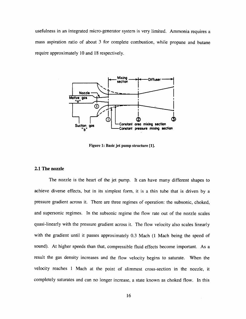
A simple jet pump structure is depicted in Figure 1. It consists of three basic

parts: a nozzle, a suction chamber, and a throat. The motive or primary gas at the input

exits from the nozzle with a high momentum, entraining the secondary gas in the suction

chamber with it and carrying the mixture through the throat to the output. The (mass)

aspiration ratio referred to in this thesis is the ratio of the mass flow rates of the

secondary to the primary flow. The entrainment happens in two steps. Near the

beginning of the throat, the secondary flow is sucked in from the suction chamber by the

lower static pressure created by the primary jet stream. Further down the throat, the

momentum from the jet stream diffuses into the secondary flow, accelerating it towards

the outlet. In the jet pump proposed here, the motive, or input, gas will be a burnable fuel

such as hydrogen, ammonia, butane, or propane, while the suction chamber is supplied

with air. While hydrogen requires a relatively low aspiration ratio for stoichiometric

combustion, it is hard to compress, and so its energy density is low. Therefore its

15

usefulness in an integrated micro-generator system is very limited. Ammonia requires a

mass aspiration ratio of about 3 for complete combustion, while propane and butane

require approximately 10 and 18 respectively.

Mixing Diff user

Nozzle-motive gas

CnD -Constont oreo mixing section"b"io Constant pressure mixing section

Figure 1: Basic jet pump structure [1].

2.1 The nozzle

The nozzle is the heart of the jet pump. It can have many different shapes to

achieve diverse effects, but in its simplest form, it is a thin tube that is driven by a

pressure gradient across it. There are three regimes of operation: the subsonic, choked,

and supersonic regimes. In the subsonic regime the flow rate out of the nozzle scales

quasi-linearly with the pressure gradient across it. The flow velocity also scales linearly

with the gradient until it passes approximately 0.3 Mach (1 Mach being the speed of

sound). At higher speeds than that, compressible fluid effects become important. As a

result the gas density increases and the flow velocity begins to saturate. When the

velocity reaches 1 Mach at the point of slimmest cross-section in the nozzle, it

completely saturates and can no longer increase, a state known as choked flow. In this

16

regime, as long as the pressure gradient is sufficient to sustain choking, the mass flow

rate will no longer scale linearly with the pressure gradient. Instead it scales linearly with

the absolute pressure at the nozzle input, while the flow velocity remains unchanged. In

other words the density of the gas changes. In nozzles with converging shape or constant

cross-sectional area, the maximum output velocity is Mach 1. In diverging nozzles, for

choked flow, the output velocity is supersonic. In this regime, the velocity will be

independent of the pressure and only a function of the nozzle geometry [4].

From a design stand point, there are three parameters that determine the required

nozzle geometry: the desired mass flow rate, the flow velocity, and the available input

pressure. If the static pressure at the output of the nozzle (i.e. in the suction chamber) is

defined to be approximately atmospheric, then for a given input pressure, the area and the

length of the nozzle will together determine both the mass flow rate and the flow velocity

at the output. For moderate flow velocities, velocity and flow rate are both roughly

proportional to cross-sectional area and inversely proportional to the length. For choked

flow and supersonic nozzles, the geometry is more complicated, and it will not be dealt

with here. Design issues that concern the interaction between the nozzle and the rest of

the jet pump structure are discussed in the next section.

2.2 The throat

As can be seen from Figure 1, the throat has two sections: the mixing section and

the diffuser. In the mixing section, the momentum of the jet stream exiting the nozzle

diffuses into the surrounding air, causing acceleration of the secondary flow. In the

diffuser the chemical species of the two gases, if they are different, continue to diffuse

17

into each other. Since the momentum diffusion is considerably quicker than the species

diffusion, the added section is sometimes necessary for complete mixing of the two

gases. The diffuser is always divergent in shape, to slow down the speed of the mixture,

thus allowing diffusion over a shorter distance. As the gas slows down, it also increases

in pressure [4].

Two considerations govern the geometry of the throat. First, the cross-sectional

area of the throat relative to that of the nozzle sets an upper limit for the achievable

aspiration ratio. Relevant calculations for this geometry are given in a later section.

Second, given a fixed area, the diffusion times can be calculated for momentum and

chemical species. If we know the flow speed, we can calculate the length of each of the

two sections of the throat required to assure complete momentum transfer to the entrained

gas and good mixing of the species.

The placement of the nozzle relative to the throat is a balance between tradeoffs.

On one hand, placing the outlet of the nozzle far away from the opening to the throat

increases the minimum flow speed at which the jet pump will function properly, because

the jet stream tends to bend off and just diffuse into the suction chamber. On the other

hand, if the nozzle is too far inside the throat, an additional pressure gradient appears

between that point and the suction chamber that adds flow resistance to the entrainment.

The intuitive solution is to place the nozzle tip exactly where the throat begins. However,

experimental data shows that the best aspiration ratio is obtained when the tip of the

nozzle is located about two nozzle diameters outside of the throat [5].

18

2.3 The suction chamber

Compared to the nozzle and the throat, the suction chamber is a relatively easy

part to design. The only strict requirement is that it should exhibit as little resistance to

the air flow as possible. In other words, for all regimes of operation of the jet pump, all

pressure gradients within the suction chamber should be very small. Depending on the

application, one may actually sometimes omit the suction chamber all together.

In some cases it may be necessary to filter the air before it reaches the throat.

Placing such a filter right at the throat will usually create too much flow resistance over

too little area. Instead, placing filters at the outer boundaries of a larger suction chamber

allows efficient filtering with negligible flow resistance.

2.4 Thesis study

All parts of this thesis deal exclusively with gas-gas jet pumps. Also, for

simplicity, all calculations and simulations are done with both the primary gases and

secondary gases being air. For heavier or lighter gases in the primary flow, the mass

aspiration ratios will change a little bit, due to small changes in diffusion properties, but

the overall theory and limiting behavior is the same. The thesis study will also not be

concerned with species mixing, since it will be assumed that the mixing can be completed

further down the system that the jet pump is connected to.

The study investigates whether jet pumps can be used in fuel controllers for

micro-generators or micro-fuel processors. The low flow rates, combined with the rather

high flow velocities, needed, demand nozzle diameters in the micron range. This is the

motivation for employing micro-fabrication techniques. The first part of this study will

19

be the ideal jet pump approximation, which turns out to be good in many large-scale

applications.

20

3. The ideal jet pump

It is instructional to study the concept of an ideal jet pump, which represents an

upper limit to the performance of jet pumps, and is a reasonable approximation under

certain conditions. The key characteristic of this idealization is the assumption that there

exists no viscous friction between the gas and the walls of the structure. Under this

assumption, it is possible to develop a relatively simple, analytical solution for aspiration

under incompressible flow conditions. This solution will be studied in two steps. It will

first be assumed that both the suction chamber and the outlet are at atmospheric pressure,

and second, a higher pressure will be added at the outlet. Both the primary and secondary

gases are assumed to be the same.

3.1 Atmospheric outlet pressure

Figure 2 below shows the simple schematic of an ideal jet pump. The figure

should be viewed as having a circular cross-section. The following three assumptions are

made:

1. All structure walls are entirely friction-less, and hence the cross-sectional

velocity profiles of developed flows are flat.

2. The velocity profiles at interface 1 are assumed to be piecewise flat, and the

structure is assumed to be long enough that the flow at interface 2 is also fully

developed.

3. The static pressure at interface 1 is assumed to be uniform over the whole

interface (for incompressible flow, this is a good assumption).

21

With these assumptions in place, the problem can be set up using simple mass and

momentum conservation laws. Both the suction gas and the outlet gas are assumed to be

at atmospheric pressure. At interface two, the total pressure of the secondary area must

be atmospheric, since the air is coming from an atmospheric reservoir, and no shaft work

has been done on it. Hence the static pressure must be equal to PATm - I pV2

Furthermore, the static pressure is assumed to be constant across interface 1, so this must

also the static pressure of the primary area.

Secondary -

Primary

Secondary - - --

Figure 2: Ideal jet pump structure.

Momentum balance:

P (As + Ap )+ pVSAs + pV2A= P2 (As + A, )+ pV 2As +A) Eq. 1

1 Vwhere P = PATm - 2VS Eq. 2

2

and P2 = PATm Eq. 3

Mass balance:

V s V2 Eq. 4pAs pAp p(As + A)

22

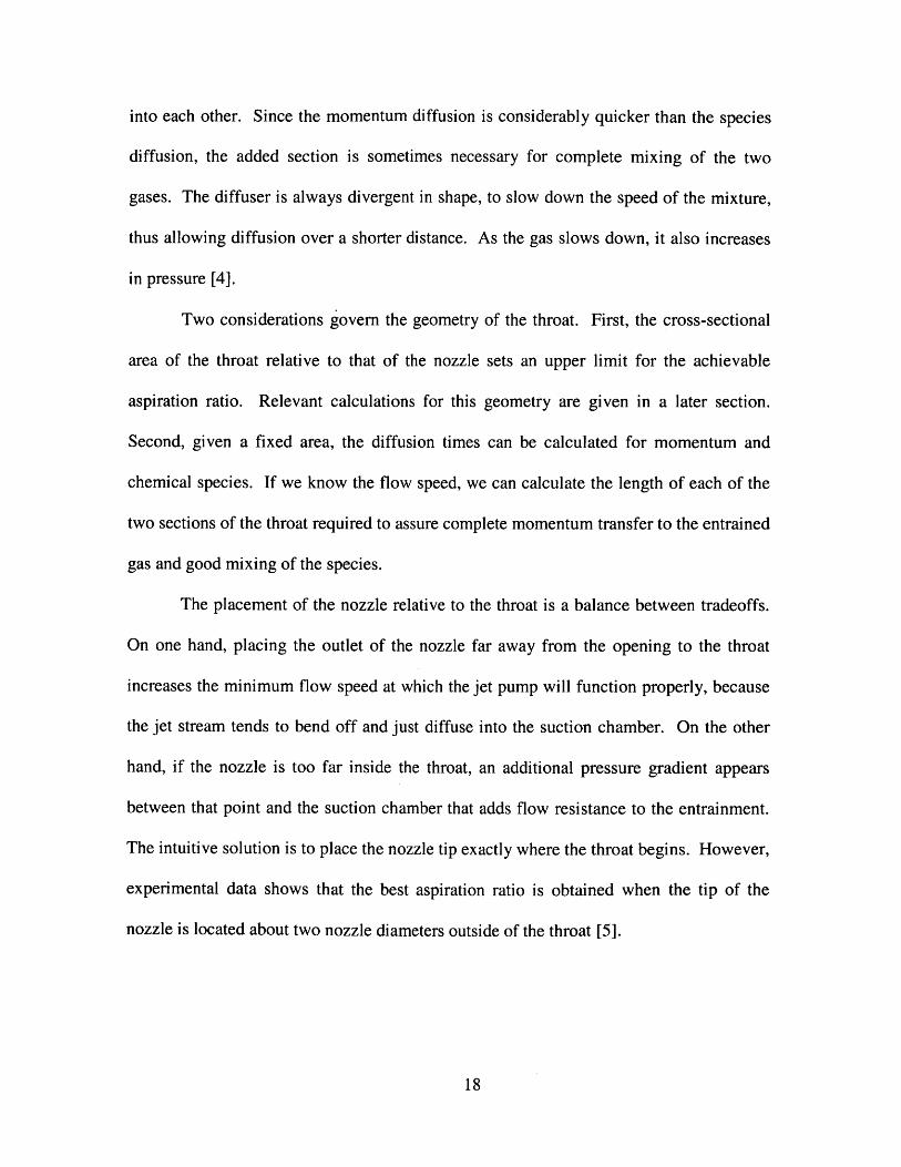
It is assumed for now that all the gases present in the system have the same

density p. By combining the two sets of equations and manipulating the expressions, one

finds that the mass aspiration ratio is only a function of the ratio of the secondary to

primary area ratio (Eq. 5). The function is plotted below in Figure 3.

-2+2 1+- +tns 2 Ap As)-- 2E Eq. 5

inAP A2

As

This dependence makes sense, since there is no loss of momentum, and no force

working against the flow in the system. Since there is no viscous friction, absolute

geometries are irrelevant. As the area ratio (As /A, ) is increased, the function

approaches a simple square root dependence, which means that there is no limit to the

obtainable aspiration ratio.

At first glance this is a very satisfying result. Aspirating enough air is just a

question of making the area ratio large enough. The problem, however, is that it is only

useful for burning in an open system, such as a Bunsen-style burner. Most closed

systems will have an internal pressure higher than the ambient. Unfortunately, as it will

be seen in the next section, even very small internal pressures can limit the performance

of a jet pump severely.

3.2 Non-atmospheric outlet pressure

If we assume that the jet pump is connected to a closed system, the outlet of the

jet pump will no longer be at atmospheric pressure but at a higher ambient pressure,

internal to the system. We can use the same analysis as in the above section with one

23

change: The outlet pressure can now be expressed as the sum of the atmospheric

pressure and some finite positive backpressure PB. In other words, Eq. 3 becomes

20

18

16

E 126

10

8

W6

4

2

0C 50 100

Area ratio: N/A,150 200

Figure 3: Aspiration ratio for an ideal jet pump with atmospheric outlet pressure.

2 PATM + PB Eq. 6

The new relationship for the mass aspiration ratio is given in Eq. 7. The mass

aspiration is now a function of both the area ratio and the primary (jet) velocity. No other

dependencies should be expected, because for fixed background (outlet) pressure and gas

density, the area ratio and the primary velocity constitute the only two independent

variables in the system.

24

I - -- - I

-

- 2+2 1+ @1+ A, As _ PB As 7S-2 As )_A_ pV_ A_)

in,. A_

As

There are two important limiting behaviors to point out in this equation. First, as

the primary velocity approaches infinity, the effect of the back-pressure is erased, and the

equation reduces to Eq. 5. Second, there is a finite, optimal area ratio for a given PB and

Vp. The peak occurs because, as the area ratio is increased, the total momentum from the

jet stream is not changed, while the total- backward force from the outlet pressure scales

linearly with the outlet area. These two effects are shown simultaneously in Figure 4.

The outlet pressure used is only 0.2 psi (1333 Pa or X 5 of an atmosphere) higher than

PATM, which shows how limiting the effect of backpressure is, and how important it is to

achieve a high primary velocity. This number for PB is the estimated pressure inside one

of the micro reactor systems. Since these equations do not hold for backward flow, all

negative aspiration ratios are shown to be zero. Furthermore, it should be noticed that the

gas flow starts becoming compressible around 100 m/s (-0.3 Mach), and that Eq. 7

therefore is no longer accurate. The real compressible solution is, however, at best

slightly better.

25

2.5

02,E

1.5

0

0.5

040

3020

10

Area ratio:A /A,0 0

Average nozzle velocity [m/s]

Figure 4: Aspiration ratios for PB = 0.2 psi (1333 Pa).

3.3 The ideal jet pump approximation

In literally all large-scale jet pumps, the flow in the throat is highly turbulent.

This is because the high velocities easily drive the Reynolds number far beyond the

critical limit of 2300 [6]. While there will certainly be boundary layers created along the

side walls of the throat, most jet pumps are built so that these layers do not become very

thick before the outlet is reached. The throat can also be built to be slightly diverging to

compensate for the boundary layer formation.

In turbulent flow, the interface between the boundary layer and the center flow is

very abrupt, and so in the center, plugged flow is typically achieved. To this flow, it

26

150

50

200

looks as if the interface to the boundary layer is a virtually frictionless wall [7]. It is for

this reason that the ideal jet pump approximation applies very well for turbulent flow.

Once the jet pump decreases in size and the flow becomes laminar, the aspiration can

only get worse, due to viscous friction. While the ideal calculations made above rely on

incompressible flow, the simulations presented in the following section take

compressibility into consideration. In theory, compressible flow can be both worse and

better than incompressible flow in a jet pump, but because of the massive reduction seen

in the aspiration ratios, the ideal approximation is still a valid upper limit.

27

4. Non-ideal jet pumps discussed and simulated

While the ideal jet pump approximation may often be good for large scale jet

pumps, the situation is rather different when the dimensions are shrunk down sufficiently.

When the diameter of the nozzle is on the order of microns, the Reynolds number for the

flow in the throat will typically be around or below the critical limit for turbulent flow in

a tube (-2300), even for high jet velocities. Therefore, the flow is laminar, and so the

idealization described at the end of the last chapter, is no longer valid. In laminar flow

there are considerable viscous losses to take into account, and the absolute geometry of

the problem has to be considered.

This chapter studies the basic loss effects and the geometry and scaling issues of

the involved. Unfortunately the problem has no simple, analytical solution under laminar

flow conditions. Therefore the reasoning is backed up by finite volume calculations (a

finite difference technique) done with CFD-ACE®. Before treating the subject further,

the simulation setup will be introduced.

4.1 Simulation setup

The flow analysis was done in CFD-ACE*.

Figure 5 below shows a drawing of the simulated structure. The nozzle and the

throat are both cylindrical, and the nozzle outlet is a certain length into the throat. All

walls are set to zero slip and isothermal conditions. The two inlets have total pressure

settings with no forced velocity direction; the secondary inlet is always at atmospheric

pressure, while the primary inlet pressure is varied. The outlet is set to a fixed pressure,

which is also varied from simulation to simulation.

28

Throat length: LT

Throat t Secondary

diameter: DT Primary Nozzle diameter: DN Outlet

Secondary

Nozzle length: LN

Figure 5: Cylindrical jet pump structure used for simulations.

The structure was simulated in a rotational symmetry. The nominal dimensions

are DN = 20 ptm, DT = 2 mm, LN = 500 pm and LT = 2 cm. The nozzle walls have a

thickness of 10 pm. Hence the nominal area ratio is slightly below 10,000. The length of

the nozzle is less important, because we are interested in the velocity at the outlet of the

nozzle, not the pressure applied to its inlet. The software was set to run a set of equations

for cylindrical geometry and compressible, non turbulent flow. The mesh was

quadrilateral. The gas used was air.

4.2 Viscous friction effects and scaling

As mentioned, at micron scale dimensions, the Reynolds number in the throat is

typically low enough that the flow is laminar, even for Mach numbers approaching 1.

This has several implications for the jet pump performance. First of all, it means that

there are significant viscous losses along the walls. Also, in regions of fully developed

flow, the velocity profiles are no longer approximately flat but parabolic.

29

-

4.2.1 The "flow in a tube" approximation

Operation of the jet pump relies on transfer of the momentum from the primary

flow to the secondary flow. Therefore, when trying to scale it properly, it is important to

know how the distance it takes for flow to become fully developed varies with scaling.

Eq. 8 below describes the distance xfd it takes for a flow in a cylindrical tube of diameter

D to develop fully at an average velocity V. While this equation is based on the

assumption that the flow velocity profile is flat at x=O, the flow situation in a jet pump is

much more complex, but it is a good order of magnitude calculation to make.

Xfd =0.05 -ReD D=0.05. VD2 [8] Eq. 8V

Ideally, fully developed flow should occur at the same relative position in the scaled tube

for a fixed velocity, i.e. xfdALT must remain constant. Therefore, if the length is scaled

down by a factor of a, the diameter must be scaled down by V. In other words, the

length and the cross-sectional area are being scaled by the same amount. Further

investigation and the simulations will show that this relationship holds quite well.

If, on the other hand, the flow is turbulent, the relationship for xfd is independent

of the Reynolds number, as shown below in Eq. 9.

10 -D! xfd 60. D [8] Eq. 9

This relationship is an empirical result, and the exact factor in front of D depends on the

situation. In this case, the length and the diameter must be scaled by the same amount for

xfd/LT to remain constant. As has already been noted, the turbulent flow regime is not

reached for very small dimensions, and this relationship will not be studied any further.

30

It is included to demonstrate that the scaling principle used for laminar flow jet pumps

does not necessarily extend to larger scales with turbulent flow.

Carrying the discussion of fully developed flow in a tube a little further, it is also

interesting to look at the flow resistance experienced by the flow. While, again, this is

not at all the flow situation seen in a jet pump, certain parts of it will experience

something crudely similar to fully developed flow.

R = 512 [9] Eq. 10;rD4

Eq. 10 shows the expression for the flow resistance in a tube with Poisseuille flow (fully

developed flow with no-slip walls). It is defined as the pressure difference over the

length L, divided by the volumetric flow rate. It is a measure of the viscous friction

losses in the tube. By applying the scaling rules established above, as the length is scaled

down by a and the diameter down by Va, R scales up by a. (As an aside, if both the

length and the diameter were scaled by the same amount, R would increase as a2 instead.)

The only conclusion that should be drawn from this, since it is a rather crude

approximation, is that as the size is scaled down, the resistance, and therefore the viscous

losses, will increase. As a consequence, the aspiration ratio will be reduced for otherwise

equal conditions.

While this very simplified view of the jet pump may be instructional, it is

important to take a closer look at the actual scenario, to get a more precise idea of what is

really happening in the jet pump. The next section proceeds with qualitative arguments,

supported by simulation results.

31

4.2.2 Momentum diffusion

The distance d over which momentum diffuses over an interval of time T, is given

by Eq. 11. v is the kinematic viscosity or the diffusion coefficient for momentum of the

gas. Its units are m2/s.

d=V5 7 Eq. 11

If we consider (which will be true for any operational regime of the jet pump) that

the velocity of the primary flow is much higher than that of the momentum diffusion,

then to the first order the speed of momentum diffusion in the radial direction will be

proportional to the square root of the primary lengthwise velocity (in other words the

amount of cross-sectional area it spreads to in the radial direction per unit time is

proportional to the lengthwise velocity). The diffusion of momentum is not, though, a

linear process, because as it diffuses, the primary flow it originated from naturally slows

down. Figure 6 shows a cartoon of this process. The lines indicate the boundary where

the momentum from the primary jet flow has reached.

Figure 6: Cartoons of momentum diffusion in a jet pump.

32

In the first of the three cartoons, the momentum just reaches the wall at the end of

the throat. This turns out to be the ideal scenario. In the second cartoon, the momentum

reaches the wall at an earlier stage, and from that point to the outlet, momentum is lost

through viscous friction to the wall. This is clearly undesirable. In the third and last

cartoon, the momentum does not reach the wall at all before the end of the throat. This is

an interesting case for a couple of reasons. In the region near the wall where the

momentum has not diffused yet, there is in fact no driving force for the secondary flow.

The lower static pressure created by the primary jet stream near the nozzle outlet, is not

only pulling air in from the secondary inlet; it is also causing a backward flow along the

walls from the throat outlet. The two last cases can clearly be obtained by either making

the throat longer or shorter, or by flowing slower or faster.

All three regimes have been simulated and graphical representations are shown

below in Figure 8, Figure 9, and Figure 10. The graphic shown is half of the jet pump

cross-section in the lengthwise direction. The bottom boundary is the center of the jet

pump, and the bottom left corner is the location of the nozzle. It is so small compared to

the rest that it is hard to see. The color indicates the values of the stream function (not

the velocity). The dimensions are the nominal ones explained in section 4.2 above. Each

graph shows the flow velocity profile at the cross-sections indicated by two connected

"plus" signs in the diagram above them. The y-coordinate is velocity in the units of m/s,

while the x-coordinate corresponds to the position along the cross-section, the center

being the leftmost point, and the wall being to the right. All three simulations use

atmospheric outlet pressure.

33

I I

1 30 _

50

10 \

Y- Coord

4-

3-

Y- Coord

2-

Y- Coord

Figure 7: Approximately optimal flow.

In Figure 7, the flow is at the velocity where the aspiration ratio is at its highest.

This turns out, as predicted, to be at the jet stream velocity where the momentum has just

diffused to the walls at the end of the throat. As the profile shows, it is not entirely fully

developed (parabolic), but the wall is certainly seeing some viscous friction beginning to

appear. The leftmost graph shows the profile just at the outlet of the nozzle. Here, no

diffusion has had time to happen, and the velocity is peaked at the center, while a quasi-

parabolic flow is coming in from the secondary inlets. The latter flow is hard to see,

because the peak at the nozzle center is so high. (It is easier to see it in Figure 9.) In the

center of the throat, the momentum has diffused over a considerable area, but it has not

yet reached the side walls.

50

-0

10

Y- Coord

0.7-

0.5-

0.3-01

Y- Coord

0.5-

-0.3

0.1

Y- Coord

Figure 8: Flow slower than optimum.

34

I I

I

II

In Figure 8, the flow has been slowed down. This allows the momentum to

diffuse to the wall earlier. Already at the center of the throat, one can see that the gas

near the wall is being accelerated. By the time the outlet is reached, the flow is fully

developed. For this specific case, roughly, the second half of the throat effectively works

as a pure cylindrical flow resistance.

130 3-

100 30- 2-D 7 0 D20- 1 -

40 10- 0-10 0 -

Y- Coord Y- Coord Y- Coord

Figure 9: Flow faster than optimum.

In the last case, Figure 9, the flow is faster than the optimum. By the time the

outlet is reached, the velocity profile looks very much like the one at the center. The

scale has been blown up to show clearly that there is a backward flow near the wall. This

negative flow is actually also slightly present at the middle cross-section, but the larger

scale was kept to show the overall profile. Although the momentum from the primary

flow never reaches the wall, the aspiration ratio is reduced due to the backward flow. An

additional effect, which is only present when the flow is compressible, reduces the

aspiration further from this point on [5].

While it is clear that the aspiration ratio decreases as the velocity is increased

beyond the optimal point, it turned out to be impossible to simulate this properly with

CFD-ACE®. The reason is that under these conditions, the outlet flow is very far from

being fully developed, and thus the fixed pressure outlet condition does not hold. A

35

sharp discontinuity would appear at the outlet, which is completely non-physical. This is

not a critical problem, since the simulations went a little bit beyond the peak before

problems arose, and the optimal regime is of most interest. Another problem that

sometimes arose, was that the simulations were not able to handle choked flow, and

therefore only velocities up to about 300 m/s could be used.

4.2.3 Viscous friction and scaling

In the laminar flow jet pump, the viscous friction can be viewed as originating

from two individual sources. The first one is that seen along the walls of the structure by

the secondary/entrained flow. This gas is sucked in by the presence of a lower static

pressure inside the throat, and that is its only driving force until it directly sees the

momentum that diffuses out from the jet stream further down the throat. The second

source is that seen by the jet stream, beginning at the point where its momentum has

reached the side wall.

The dip in the static pressure, which was also described earlier in this document,

is shown in the form of a simulation result in Figure 10 below. The plots show static

pressure along three lengthwise cross-sections between the crosses in the figure (zero

corresponds to atmospheric pressure, units are Pa). The leftmost plot corresponds to the

lowest cross-section (closest to the center of the jet pump), and so forth. The sharp dip in

this plot corresponds to where the nozzle outlet is located. The other two graphs clearly

show the smooth dip in pressure, which is the initial driving force for the secondary flow.

All three graphs also show a small peak in pressure near the outlet. It corresponds to a

short region of close to fully developed flow, which is the second source of viscous

36

friction. If the flow were faster or the throat were shorter, this region would disappear,

and the pressure would rise monotonically to the atmospheric outlet.

0 0

-0.3 - -0.3-2 -0.6 -0.6~

3-0.9 F-0.9

X-Coord X- Coord X-Coord

Figure 10: Pressure profiles in the jet pump.

The first source of viscous losses is impossible to eliminate, since it is seen

throughout the whole length of the throat. However, it is likely to be smaller than the

second one, because the secondary flow velocity is not very high until the primary flow

momentum diffuses into it. As described in the previous paragraph, the second source of

losses can be eliminated by shortening the throat or speeding up the flow. This means

that for any given structure, there is an optimal flow velocity. At this velocity, the second

source of viscous losses will be mostly absent. As the structure is then scaled down, the

increase in the losses from the first source will reduce aspiration ratio.

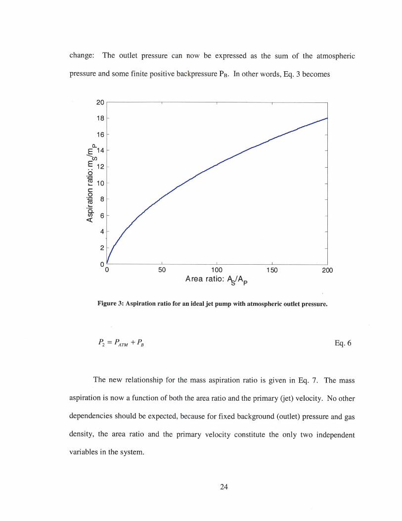
Figure 11 below shows a graph of the aspiration ratio versus nozzle velocity for

the nominal jet pump and for a jet pump scaled down by 10, according to the scaling

rules previously established (LT is divided by 10 and DT is divided by the square root of

10).

37

80

70

60$50

$40

30

20

10

00 250 300 350

-+- Nominal -m- Scaled down by 10

Figure 11: Laminar flow jet pump scaling.

As we can see, the optimal point is almost at the same velocity, which confirms

that the scaling rules hold very well. More importantly, as expected, the maximum

aspiration ratio has decreased from about 70 to about 65. It does not decrease by

anywhere near a factor of 10, but the flow resistance approximation was not expected to

be very accurate. Besides, the first source of viscous losses is not extremely important

compared to the primary flow. In both cases, the secondary to primary area ratio is about

10,000. An ideal jet pump with this area ratio would have an aspiration ratio of about

140, so even though a large scale jet pump may not do quite as well as that, it is clear that

the viscous friction in the laminar jet pump is severely limiting the performance.

As an additional observation, it is possible to have a negative aspiration ratio even

though the outlet pressure is atmospheric. The reason for this is that if the flow is slow

enough, it may see less flow resistance in turning around and going back out the

38

50 100 150 200

Nozzle velocity [m1s]

secondary inlet, than it sees going down the throat. This scenario is depicted in Figure 12

below by the stream function lines. Only a section around the nozzle area is shown.

Figure 12: Negative aspiration with atmospheric outlet pressure.

Lastly, Figure 13 has been included to show two effects obtained from the

simulations. The figure has four sets of data points. They correspond to 1) the nominal

jet pump, 2) an identical pump with half the throat length, 3) the latter with a throat

scaled up by 2 (the nozzle is not changed at all), and 3) the same pump with a throat

scaled up by 4. Because the scaling rules have been followed (the scaling factors are for

the lengths and the diameters are scaled by the square root), the last three jet pumps were

expected, to first order, to have optimum aspiration at the same velocities.

39

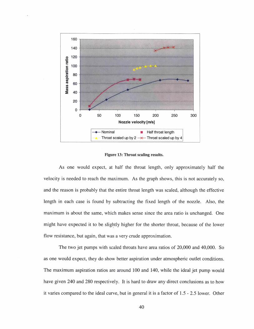
Figure 13: Throat scaling results.

As one would expect, at half the throat length, only approximately half the

velocity is needed to reach the maximum. As the graph shows, this is not accurately so,

and the reason is probably that the entire throat length was scaled, although the effective

length in each case is found by subtracting the fixed length of the nozzle. Also, the

maximum is about the same, which makes sense since the area ratio is unchanged. One

might have expected it to be slightly higher for the shorter throat, because of the lower

flow resistance, but again, that was a very crude approximation.

The two jet pumps with scaled throats have area ratios of 20,000 and 40,000. So

as one would expect, they do show better aspiration under atmospheric outlet conditions.

The maximum aspiration ratios are around 100 and 140, while the ideal jet pump would

have given 240 and 280 respectively. It is hard to draw any direct conclusions as to how

it varies compared to the ideal curve, but in general it is a factor of 1.5 - 2.5 lower. Other

40

140

o 120

1000

280

60

2 40

20

00 50 100 150 200 250 300

Nozzle velocity [mfs]

-+- Nominal M Half throat lengthThroat scaled up by 2 -x-- Throat scaled up by 4

than viscous losses, the variation is probably due to compressible flow effects at the

higher velocities.

4.3 Outlet pressures

So far the simulations have only used atmospheric outlet pressures, so that the

effects of viscous friction and scaling could be more readily isolated and identified.

Because of the very large are ratios employed until now, applying even very low outlet

pressures would give backward flow in most situations. Therefore, a much smaller jet

pump was simulated. It had the following dimensions: DN = 20 jim, DT = 200 jim, LN =

500 jim and LT = 1.5 mm. The nozzle walls again have a thickness of 10 pm, so the area

ratio is 96. The simulated outlet pressures, PB (above atmospheric pressure), were 0, 50,

and 400 Pa. These are too low for any applications of interest, but they are meant to be

instructional in making a comparison to the ideal jet pump.

Figure 14 below shows the simulation results. Although the 400 Pa case does not

reach its optimum aspiration ratio before the velocity limit for choked flow is reached,

the trend from the three cases is clear. Increased pressure reduces aspiration drastically,

and the optimum velocity increases. These trends are as expected from the analytical

solutions, although they did not predict the reduced aspiration for higher velocities. That

discrepancy is due to the ideal assumptions the flow was always fully developed by the

time it reached the outlet, and there was no viscous friction.

41

4.5-

. 4

.03.50cc 3

0 2.5

fA 1.5 -a

0.5

0

Nozzle velocity [n/s]

-- b=0 Pa -- Pb=50 Pa P b=400 Pa

Figure 14: Outlet pressures above atmospheric.

Quantitative comparisons can be made for the 0 and 50 Pa cases. In the

simulations the maximum aspiration ratios are 4.25 and 3.5 respectively, the latter

obtained at a velocity of about 220 m/s. In the ideal case, this would correspond to

aspiration ratios of 12 and 11.4 respectively. Ratio wise these correspond quite well,

although the case with backpressure does a little worse. The 400 Pa case should be

roughly 10 for the ideal aspiration, while it here is approximately 2. It indicates a trend

of higher outlet pressures having a higher impact on laminar jet pumps than on ideal

ones, although it is hard to separate how much of this behavior is caused by compressible

effects. It is important, however, to acknowledge that the effect of backpressure

qualitatively appears to be the same in the two cases, and that the ideal case, as expected,

is an optimistic estimate.

42

5. Experimental data

Early in the work on this thesis, a set of micro-scale jet pumps were fabricated

and tested. The design, as will be discussed, had many flaws, but it was an instructional

experiment nonetheless. The first generation micro-fabricated jet pumps were built in the

M.I.T Microsystems Technology Laboratory (MTL) and tested in the Jensen-group

chemical engineering laboratory.

5.1 The design and process flow

Figure 15 below shows a picture of one of the first generation micro-fabricated jet

pumps. The nozzle is about 20 pm wide, while the throat is 2 mm wide at the thinnest

point and about 2 cm long. The depth of the pattern seen is about 350 gm.

ThroatSecondary inlet S

Outlet

Primary inlet

Figure 15: Picture of a micro fabricated jet pump.

The device was made by etching the features into a silicon wafer using DRIE

(Deep Reactive Ion Etching), then etching the inlet and the outlet from the back side of

the same wafer, and finally bonding a pyrex glass wafer to the top to close off the

43

chambers. The process flow is shown in Figure 16 below. The cross-section is taken as

depicted in Figure 15. The simple process was relatively free of problems, and a wafer

with 20 devices with varying features was successfully fabricated.

A M - M B DRIE etch jet pumpstructure in Si wafer.

DRIB etch inlet and outlet throughN o ma wfrom the back side.

Nozzle inlet

pyrex Anodically bond pyrex wafer toSi wafer.

Figure 16: Process flow (not to scale).

Inspection of the fabricated devices revealed that the nozzles were less deeply

etched than the rest of the structure. They were about 250 gm instead of 350 pm.

Uniformity across the wafer was small enough that it was not really an issue, since small

variations in depth were unlikely to make much difference.

44

5.2 Testing

A diagram of the test setup is shown in Figure 17.

Flow-meter Jet pump Bubble

Air columntank

M.... ..... Pressure

gauge

Figure 17: Test setup.

The jet pump was driven by a 1000 sccm (standard cubic centimeters per minute)

flow meter, which in turn was fed by a pressurized air tank. The pressure gauge allowed

measurement of the nozzle inlet pressure of the jet pump, and the bubble column was

used to manually (visually) measure the flow rate out of the jet pump outlet. Tubing

connections were made to the jet pumps by gluing ferrels to the outlets and then gluing

1/ 16th inch tubing to the ferrels. The bubble column was assumed to approximate an

atmospheric output. The testing was done with air as both the primary and secondary

inputs. While the volume aspiration would be quite different for gases of different

weight, the mass aspiration ratios should be very similar.

Devices with a variety of feature sizes were tested, and the results from two of

these are shown in Figure 18. The results from two pumps of different nozzle width were

chosen to illustrate the only consistently observable behavior found among the

experiments. This behavior is that a nozzle twice as wide (i.e. with twice the cross-

sectional area) needs about twice the flow rate to achieve the same velocity in the throat,

or in other words to achieve the maximum aspiration ratio. The x-axis shows the flow

45

rate, not velocity, but even though these are not linearly related over all flow velocities,

the shape of the curves clearly indicate the effects discussed in the previous section.

Disappointingly, the aspiration ratio was very low.

2

1.5 -

L-u- 40 urn nozzle width0.5-

0

Input flow rate [sccm]

Figure 18: Selected experimental results.

Despite an area ratio of about 100, the aspiration ratio was at best only around 1.5.

Two things can most probably explain this performance. First, as a consequence of the

process flow, the whole jet pump is essentially a two dimensional structure. The nozzle

extends from the "floor" of the device and to the "ceiling", resulting in viscous losses to

those two walls from the moment the primary flow leaves the nozzle. The fact that the

flow must make a right-angled turn to exit the throat certainly doesn't help either.

Second, the thin tubing necessary to connect the output to the bubble column, contributed

to a high output pressure at higher flow rates. From the flow rates, and the geometry, the

pressure gradients created over the used length of tubing were estimated for each data

point and are shown below in Figure 19.

46

1.6- 4000

1.4 3500 e

1.2 3000 2

0 7111. 2500 4)

.0.8 2000 cL

S0.6 1500 '

0.4 -1000 E

0 00 100 200 300 400 500 600

Input flow rate [sccm]

--- Aspiration -m- Pressure

Figure 19: Estimated outlet pressure for the 20 ptm nozzle jet pump.

The increasing outlet pressure certainly partly explains the steep fall in the

aspiration ratio for higher flow rates. In fact it already has some effect at the optimum

point. It is virtually impossible to make a quantitative comparison to the ideal jet pump

approximation, because only the first data point in Figure 19 has a slow enough nozzle

velocity to be incompressible, and from the fourth data point the flow is choked.

Shortening the tubing, which was typically less than 3 cm long, did increase aspiration.

Although the aspiration ratio did not increase by much (it never went above 2), it had a

much bigger effect than the varying throat widths and nozzle placements that the

different devices exhibited. The varying structural features did not give any consistent

variation in aspiration ratio, and it was concluded that the differences observed were

mostly due to differences in outlet tubing lengths.

47

6. A possible improved design

In sketching out a better design for micro-scale jet pumps, the conclusion seems

to be that it is necessary to go beyond perfecting the conventional design. The key

feature to strive for is ideality: the flow must look as much as possible like that in an

ideal jet pump.

Once it has been established that the flow in the jet pump will be laminar, it is

inevitable to have viscous losses at the wall. The hope is that one might be able to create

something like a plugged flow further away from the walls. One possible approach to

this is to use a two-dimensional array of nozzles instead of just one nozzle. Figure 20

shows a cross-sectional cartoon of a multi-nozzle array. Only 3x3 nozzles are depicted,

but in reality l0x10 might be a more reasonable number.

L......J

Figure 20: Cross-section of a multi-nozzle array jet pump.

The nozzles are depicted with a finite wall thickness. For simplicity of the

argument the outer tube is taken to be square. It could just as well have been circular,

with a slightly different arrangement of the nozzles. The thought behind this design is

that far enough from the outer walls, the half-way boundary between the nozzles (one of

them is depicted as a dotted line) looks like a symmetry boundary. A symmetry

48

boundary in practice serves the function of a slippery wall, because there is no normal

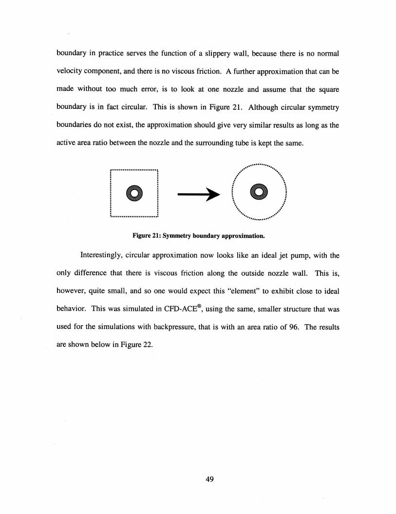
velocity component, and there is no viscous friction. A further approximation that can be

made without too much error, is to look at one nozzle and assume that the square

boundary is in fact circular. This is shown in Figure 21. Although circular symmetry

boundaries do not exist, the approximation should give very similar results as long as the

active area ratio between the nozzle and the surrounding tube is kept the same.

-.....->

Figure 21: Symmetry boundary approximation.

Interestingly, circular approximation now looks like an ideal jet pump, with the

only difference that there is viscous friction along the outside nozzle wall. This is,

however, quite small, and so one would expect this "element" to exhibit close to ideal

behavior. This was simulated in CFD-ACE*, using the same, smaller structure that was

used for the simulations with backpressure, that is with an area ratio of 96. The results

are shown below in Figure 22.

49

I-

CL

12

10

8

6

4'

2

00 100 150 200

Nozzle velocity [mTfs]

Figure 22: Simulated performance of a semi-ideal jet pump "element".

For this area ratio the ideal aspiration ratio is 12, and for the "element" it is almost

10, which is only off by 1/6. This is also more than twice as good as the case where the

walls did have viscous friction. At a first glance, this looks like a reasonable approach to

making laminar flow jet pumps more ideal.

There are a few important facts to notice about the multi-nozzle array

before drawing any conclusions. In the sections of the array that lie near the sidewall, the

symmetry condition will obviously not hold, and the velocity will effectively be zero at

the wall. Also, if the throat were very long, the flow would eventually become fully

developed across the whole throat cross-section. But as long as the throat is made short

enough, these effects will not show up except near the wall. Fortunately the throat can be

kept short, because the nozzles will be very close together, and the length it takes for the

momentum to diffuse to the symmetry boundary for each "element" is therefore much

50

50

shorter than the length it takes for the flow to fully develop in the throat. Essentially the

flow at the throat outlet can then be viewed as plugged.

Another thing to keep in mind is that the array of nozzles should have the same

flow rate as the single nozzle, and they must therefore be very small (in cross-sectional

area. Many tiny nozzles close together in an array is a concept that strongly suggests

micro-fabrication. The outline for a possible design/process flow is shown below in

Figure 23.

(1)

-- --- ( 3 )

Figure 23: Nozzle array process flow (not to scale).

51

In Figure 23, part (1) shows the two separate silicon wafers needed for the

fabrication. The top wafer needs to be etched from both sides by for example DRIE. The

bottom wafer only needs to be etched through from one side, but the etch needs to be

quite straight, so DRIE is probably the way to approach here too. Part (2) shows the view

of the top (left) and bottom (right) view of the top wafer, to illustrate that the etched

pattern is actually a network of intersecting channels. The holes etched from the top

come through at the intersections of these channels. The wafers are then bonded

together, and silicon nitride is deposited everywhere, say at a thickness of around two

microns [10]. Finally a hole is etched through both wafers by using for instance fluorine,

releasing the silicon nitride structure in this area. The result is a freestanding network of

silicon nitride tubes [10] that feed to a set of nozzles. A throat needs to be placed at the

top of the device, and then, once fluid connections are made to the inlets at the bottom,

this turns to a multi-nozzle array jet pump.

A few comments should clear up the most immediate questions. First, the fluid

connections on the backside can be networked in to one instead of many, easing the

connection task. Second, the nozzles are depicted as diverging at the ends. How this

would be made in practice, in a well-controlled fashion, is not entirely clear, but the

purpose is to allow supersonic exit velocities. As it has been shown in the theoretical

calculations, even for high velocities, with the backpressures one is likely to have in a

micro fuel processor, subsonic jet pumps will not be able to meet the aspiration specs.

Therefore it is probably necessary to achieve supersonic nozzle velocities to have a large

enough driving force.

52

The design and process suggested are far from being well developed, and they are

both in need of much work if they are to be realized. The process flow itself, is also not

trivial to do. It should also be pointed out that there is no guarantee at all that this kind of

a structure would actually achieve the goals of mass aspiration ratios as high as 18. It

should be an interesting topic for future work nonetheless.

53

Conclusion

The need for a carburetor for a micro-generator system motivated this study of

micro-scale jet pumps. Jet pumps require a high primary jet velocity to pump against a

pressure at high aspiration ratios, and that combined with the need for very low flow

rates, forced the dimensions to be shrunk down. It was first shown that even with an

ideal, frictionless jet pump, it would be hard to achieve the necessary aspiration ratios, for

instance for butane. Furthermore, the discussion and simulations have established that

because the flow in these small jet pumps is generally laminar, viscous friction causes

absolute geometries and scaling to influence the aspiration ratio. At any given geometry

and backpressure, there is an optimal flow velocity at which the aspiration ratio reaches

its maximum. Micro-scale jet pumps must therefore be carefully designed around this

point. The simple conclusion to draw from this is that although the ideal jet pump can be

taken as an upper limit to performance of micro-scale jet pumps, they will generally

perform much worse.

A set of first generation micro-scale jet pumps were micro-fabricated and tested.

These devices are clearly not usable for micro fuel processor applications for two

reasons. First, the aspiration ratio is too low for any purposes of interest. It is in some

cases sufficient for the burning of hydrogen, but as explained, hydrogen is not a desirable

input gas. For more useful gases, the micro-fabricated devices are useless, because most

of the gas will pass through the generator uncombusted. Second, the flow rate is too

high. While a 1 Watt micro-generator would require about 0.5 sccm of butane, the

fabricated jet pumps operated optimally at around 100 sccm. Additionally, these jet

pumps were tested at atmospheric output conditions (although the tubing added some

54

unwanted backpressure), which means that even these mediocre results are overly

optimistic.

No doubt, many improvements could be made to the jet pump design. Creating a

cylindrical design would be a good start. However, as was seen in the discussion on

laminar flow jet pumps, it is very limited what can be done with the viscous friction

along the side walls. It is necessary to come up with a design that will make the flow in

the jet pump resemble that of an ideal structure, with no viscous friction. A proposal for

such a design was given in the last section. Multiple nozzles would assure quick

momentum diffusion and locally ideal behavior. The ideal jet pump calculations show

that it would also be necessary to make the nozzles supersonic. This would be an

interesting device to model and possibly build, but it is beyond the scope of this thesis. It

is recommended that any such work begin with a study of how promising ideal,

supersonic jet pumps are in the first place.

55

References

[1] R. H. Perry, D. Green, ed., Perry's Chemical Engineers' Handbook, 6' edition,McGraw-Hill Inc., New York, 1984.

[2] F. Aerstin, G. Street, Applied Chemical Process Design, Plenum Press, NewYork, 1989.

[3] M. M. Denn, Process Fluid Mechanics, Prentice Hall Inc., New Jersey, 1980.

[4] W. L. McCabe, J. C. Smith, P. Harriott, Unit Operations of ChemicalEngineering, McGraw-Hill Inc., New York, 1993.

[5] W. E. Francis, M. L. Hoggarth, J. J. Templeman, "The Design of Jet Pumps andInjectors for Gas Distribution and Combustion Purposes", Symposium on JetPumps and Ejectors, pp. 8 1-96, 1972.

[6] James A. Fay, Introduction to Fluid Mechanics, MIT Press, Cambridge,Massachusetts, 1994.

[7] H. Schlichting, Boundary-Layer Theory, McGraw-Hill Inc., New York, 1979.

[8] F. P. Incropera, D. P. DeWitt, Fundamentals of Heat and Mass Transfer, JohnWiley & Sons Inc., New York, 1996.

[9] S. D. Senturia, Microsystem Design, Kluwer Academic Publishers, Boston, 2001.

[10] L. R. Arana, et al, "A Microfabricated Suspended-Tube Chemical Reactor forFuel Processing", IEEE MEMS 2002 Conference, Jan. 20-24, Las Vegas, NV.

56

Appendix A: Equation derivations

The following is the derivation of Equation 5. Combining Equations 1-3 we get:

-I pV' (As + A, )+ pVAs + pVA, - pV 2 (As + A,)=02

Next, insert the equalities from Equation 4:

_ 2 A S + A + 1 +Ih (hs + th2 02s pAS pAs pAp o(As + Ap)

S2 1 1 As + A p A IsI As 2 As2 As + Ap

-2As + A,

A~rA2

P AP As + Ap

Multiply each side by s p

P

hS_ AS+AP I(AS+AA)2

Ih As 2 As2mP Ls

2Al A 1A 2

I + p I IP i 1 2-srh 2 As 2 As 2 As th

-1 -2----+ [A A 11-0thp [ A,

As+1_1 =0IAp

A(J- 2 t( +=0

thp 2

Apply the quadratic formula:

mhs

mh p

2AsAp

2- CAnd finally choose the plus sign, and get Equation 5:

57

2 ±2 1+ - I I+2

-2+2 1+ (As+ A2 1Ap As)_

1+AP)As

Next follows the derivation of Equation 7, which is very similar to the previous one. The

only difference is that the addition of the backpressure (Equation 6) gives the following

first equation:

1 22 5 A,,z + Ih (ilS + th P )2 PA )-$ Ih2 AS + AP + rh P & h12s pAS pAs pA, p(As + A,)

Rearrange:

h2F 1 I As +AP 1 2 thshr, *2 [i IAs 2 A As+A,,j As+A m AP As +Ap

As before multiply both sides by s 2p

mh

SA, 2 I-2ths +As+A 1th 2 As 2 As M,, _ A,

in .+ & 1 A, A - ths + As,h2 As 2 As 2Asjiz A, B

Li 2 I fhis

iii,,

PB (AS + ) 2

ri,

(AS + A, )2

p 2APV2

2

A s _P (As 1

AP pV(Ap= 0

Applying the quadratic formula and simplifying, Equation 7 is obtained:

58

= PPB (As + Ap)

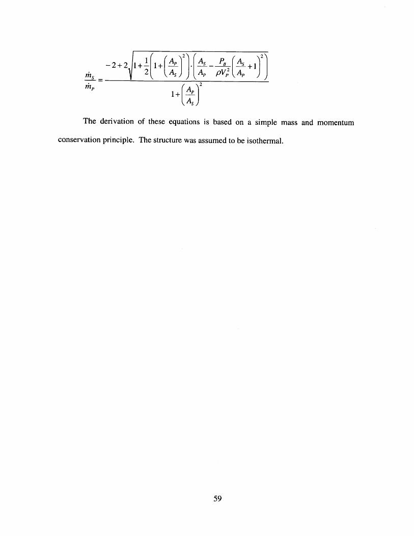
-2+ 22-2+ 2 1+ 1 1+ (A,) As -PB (s +1

2 As ) A pV,2 A )

MP+ A,As

The derivation of these equations is based on a simple mass and momentum

conservation principle. The structure was assumed to be isothermal.

59

Appendix B: Mask Drawings

Maski: Front side jet pump structure pattern.

60

0 0

0 0 0 0 0 0

0

0

0

0

0

0

0

0

Mask 2: Back side inlet and outlet pattern.

61

0 0 0

0

0

00 0

o oo

Appendix C: Process flow

The devices were fabricated in the MIT Technology Research Laboratory (TRL).

The starting material was one 4" Silicon, double-side polished wafer and one Pyrex glass

wafer, both 500 pm thick.

Detailed process flow:

Front side photolithography on Silicon wafer

Etch front side (depth 350 pim)

Strip photoresist

Back side photolithography on Silicon wafer

Etch through wafer from back side

Strip photoresist

Pre-bonding clean of pyrex wafer

Bond pyrex to front side of Silicon wafer

Separate device dies

Mask 1

DRIE

Piranha* for 10 min.

Mask 2

DRIE

Piranha* for 10 min.

Piranha* for 10 min.

Anodic bond

Die-saw

* Piranha: 3 H2 SO4: 1 H20 2

I~

62

1.

2.

3.

4.

5.

6.

7.

8.

9.