Purdue UniversityPurdue e-Pubs

ECE Technical Reports Electrical and Computer Engineering

7-1-2009

A Study of Meta Learning for RegressionM. Fatih AmasyaliYıldız Technical University

Okan K. ErsoyPurdue University - Main Campus, ersoy@purdue.edu

Follow this and additional works at: http://docs.lib.purdue.edu/ecetrPart of the Electrical and Computer Engineering Commons

This document has been made available through Purdue e-Pubs, a service of the Purdue University Libraries. Please contact epubs@purdue.edu foradditional information.

Amasyali, M. Fatih and Ersoy, Okan K., "A Study of Meta Learning for Regression" (2009). ECE Technical Reports. Paper 386.http://docs.lib.purdue.edu/ecetr/386

A Study of Meta Learning for Regression

M.Fatih Amasyalı1 and Okan K. Ersoy2 1mfatih@ce.yildiz.edu.tr, Yıldız Technical University

Computer Engineering Department Istanbul, 34349, Turkey

2ersoy@purdue.edu, Purdue University School of Electrical and Computer Engineering

Indiana, 47907, USA

Abstract In regression applications, there is no single algorithm which performs well with all data since the performance of an algorithm depends on the dataset used. In practice, different algorithms / approaches are tried, and the best one is selected in each application. It is meaningful to ask whether there is a different way instead of running such tedious experiments. In meta learning studies, one investigates clues for the performance of an algorithm over a dataset using several features of the dataset. In this context, it is important to estimate which dataset features (meta features) are most significant for the performance of the algorithm. In the literature, meta learning studies mostly specialize to classification problems. In this study, meta regression problems are comprehensively studied on 3 big dataset collections (totally 181 datasets). New and existent meta features (about 300) are used. The relationships between the datasets and the algorithms are investigated. Several relations are found between meta features and related performances. The created meta datasets are made available to interested researchers.

1. Introduction In the field of machine learning, there is no single algorithm which performs better than other algorithms for all datasets. Algorithm (model) selection is usually made by trial and error. A new approach called “Meta Learning” has recently been developed to replace the trial and error approach to choose the best set of algorithms given a dataset. In this approach, a matrix called meta dataset is formed. Its rows consist of samples (datasets), and its columns consist of the features of the datasets called meta features. The aim here is to estimate the performance of an algorithm as a function of the meta features of a dataset. Meta features can be organized in groups. In this paper, six groups of meta features have been used. See Sections 2 and 4 for the details of the meta features. There can be several uses of a meta dataset. A metadataset can be used to predict the performance of an algorithm with a given dataset. Similarly, a meta dataset can be used to predict the best performing algorithm with a given dataset. Increasing the examples of a meta dataset can be possible. Thus, a ‘machine learning expert system’ can be developed using the meta datasets. Meta datasets can also give clues for finding better performing algorithms. Almost all studies in the meta learning literature have handled classification problems. There is not any comprehensive study on regression problems. For this reason, in this study the regression problems in terms of meta-learning have been examined. 2. Related Works Previous meta learning studies generally involve meta classification problems. In Table 1, selected studies are comparatively shown and summarized. Table 1. Summary of previous works in meta learning. Reference Aim Used Meta Features Type and

number of datasets

Short Description

(Fürnkranz et all., 2001)

Meta classification

Landmarks’ performance relative to each other, subsampling landmarks, decision tree features

48 real world datasets

Using only landmarks (absolute or relative etc.) as meta features is not successful.

(Bensusan et all., 2000b)

Meta classification

Decision tree features - Experiments are not included.

(Kalousis et all., 2000)

Meta classification

57 statistical features 47 UCI datasets

Superior classifier names out of two classifiers are used as labels of meta dataset.

(Kalousis et all., 2003)

Measuring the distances between datasets having different number of features

Statistical and information theoretical features

103 real world datasets

Proposed simK, single linkage and average linkage approaches are compared and it is shown that all of them have better performances than simple averaging.

(Carrier, 2005)

Meta classification

Statistical and information theoretical features, landmarks, decision tree features

52 UCI datasets

Experiments are not included.

(Todorovski et Meta Statistical and 65 UCI A decision tree is induced whose

all., 2002a classification information theoretical features, landmarks,

datasets leaves include the classifiers’ performance order.

(Todorovski et all., 1999),

Meta classification

Statistical and information theoretical features

20 UCI datasets

A set of rules shows which classifier is better out of 3 classifiers used.

(Gama et all., 1995)

Meta classification

Statistical and information theoretical features

20 UCI datasets

Algorithm performances are predicted by regression, model tree and instance based models. None of the models have better performance than others statistically.

(Todorovski et all., 2002b),

Meta classification

56 statistical and information theoretical features

65 UCI datasets

A selected subset of meta features by wrapper type feature selector is used in prediction of algorithms’ performances. Using subset instead of all set has better prediction performances.

(Peng et all., 2002),

Meta classification

Statistical and information theoretical features, landmarks, decision tree features

47 UCI datasets

Meta features based on decision trees have better performance than other types of meta features. A selection process is applied over meta features, but performance does not increase.

(Brazdil et all., 2003)

Meta classification

Statistical and information theoretical features, landmarks

53 datasets

Obtained relative performances of classifiers.

(Bensusan et all., 2001),

Meta classification

Statistical and information theoretical features, landmarks

65 UCI datasets

Landmarks have better performance than statistical features.

(Ali et all., 2006)

Meta classification

Statistical and information theoretical features

100 UCI datasets

A set of rules shows which classifier is better out of 8 classifiers used.

(Soares et all., 2004

Parameter tuning for regression problems

Statistical and information theoretical features

42 datasets

SVM’s kernel width parameter was estimated by meta features.

Our study Meta regression About 300 Statistical and information theoretical features, landmarks, decision tree features

60 UCI + 41 drug design + 80 artificial datasets

See Section 5.

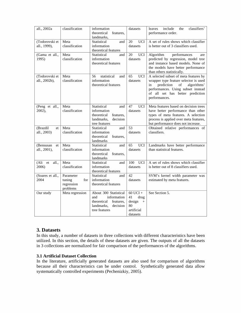
3. Datasets In this study, a number of datasets in three collections with different characteristics have been utilized. In this section, the details of these datasets are given. The outputs of all the datasets in 3 collections are normalized for fair comparison of the performances of the algorithms. 3.1 Artificial Dataset Collection In the literature, artificially generated datasets are also used for comparison of algorithms because all their characteristics can be under control. Synthetically generated data allow systematically controlled experiments (Pechenizkiy, 2005).

In meta regression experiments, 80 artificially generated datasets have been used. In the literature, The Friedman function is one of the most used functions for data generation (Friedman, 1999). Friedman function includes both linear and non-linear relations between input and output. A normalized noise (∈) is also added to the output. The Friedman function is given by

∈+++−+= 542

321 *5*10)5.0(*20)**sin(*10 xxxxxpiy (1)

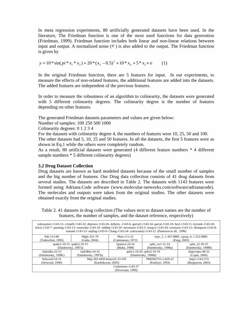
In the original Friedman function, there are 5 features for input. In our experiments, to measure the effects of non-related features, the additional features are added into the datasets. The added features are independent of the previous features. In order to measure the robustness of an algorithm to colinearity, the datasets were generated with 5 different colinearity degrees. The colinearity degree is the number of features depending on other features. The generated Friedman datasets parameters and values are given below: Number of samples: 100 250 500 1000 Colinearity degrees: 0 1 2 3 4 For the datasets with colinearity degree 4, the numbers of features were 10, 25, 50 and 100. The other datasets had 5, 10, 25 and 50 features. In all the datasets, the first 5 features were as shown in Eq.1 while the others were completely random. As a result, 80 artificial datasets were generated (4 different feature numbers * 4 different sample numbers * 5 different colinearity degrees) 3.2 Drug Dataset Collection Drug datasets are known as hard modeled datasets because of the small number of samples and the big number of features. Our Drug data collection consists of 41 drug datasets from several studies. The datasets are described in Table 2. The datasets with 1143 features were formed using Adriana.Code software (www.molecular-networks.com/software/adrianacode). The molecules and outputs were taken from the original studies. The other datasets were obtained exactly from the original studies.

Table 2. 41 datasets in drug collection (The values next to dataset names are the number of features, the number of samples, and the dataset reference, respectively)

yokoyama1-1143-13- cristalli-1143-32- depreux-1143-26- doherty -1143-6- garrat2-1143-14- garrat-1143-10- heyl-1143-11- krystek-1143-30- lewis-1143-7- penning-1143-13- rosowsky-1143-10- siddiqi-1143-10- stevenson-1143-5- strupcz-1143-34- svensson-1143-13- thompson-1143-8-

tsutumi-1143-13- uejling-1143-9- Chang-1143-34- yokoyama2-1143-12 (Patterson et all., 1996)

Pah-113-80 (Todeschini, 1995)

Pdgfr-321-79 (Guha, 2004)

Phen-111-22 (Cammarata, 1972)

topo_2_1-267-8885- yprop_4_1-252-8885 (Feng, 2003)

qsabr1-10-15- qsabr2-10-15 (Damborsky, 1997a)

Qsartox-24-16 (Blaha, 1998)

qsbr_rw1-51-14 (Damborsky, 1998a)

qsbr_y2-20-25 (Damborsky, 1998b)

Qsbralks-22-13 (Damborsky, 1998c)

Qsfrdhla-34-16 (Damborsky, 1997b)

qsfsr1-10-20- qsfsr2-10-19 (Damborsky, 1998d)

Qsprcmpx-40-22 (Cajan, 2000)

Selwood-54-31 (Selwood, 1990)

Mtp-203-4450 benzo32-33-195 (Karthikeyan, 2005)

PHENETYL1-629-22 (Kubinyi, 1993)

mtp2-1143-274 (Bergstrom, 2003)

Carbolenes-1143-37 (Silverman, 1999)

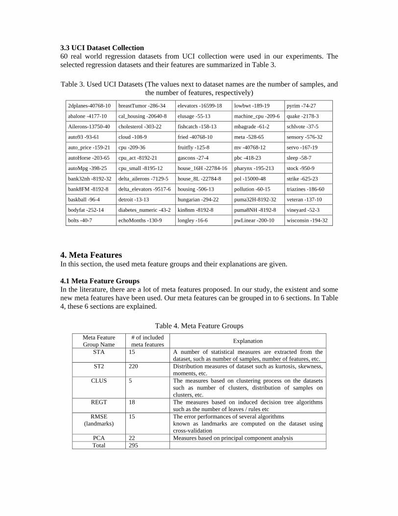
3.3 UCI Dataset Collection 60 real world regression datasets from UCI collection were used in our experiments. The selected regression datasets and their features are summarized in Table 3.

Table 3. Used UCI Datasets (The values next to dataset names are the number of samples, and the number of features, respectively)

2dplanes-40768-10 breastTumor -286-34 elevators -16599-18 lowbwt -189-19 pyrim -74-27

abalone -4177-10 cal_housing -20640-8 elusage -55-13 machine_cpu -209-6 quake -2178-3

Ailerons-13750-40 cholesterol -303-22 fishcatch -158-13 mbagrade -61-2 schlvote -37-5

auto93 -93-61 cloud -108-9 fried -40768-10 meta -528-65 sensory -576-32

auto_price -159-21 cpu -209-36 fruitfly -125-8 mv -40768-12 servo -167-19

autoHorse -203-65 cpu_act -8192-21 gascons -27-4 pbc -418-23 sleep -58-7

autoMpg -398-25 cpu_small -8195-12 house_16H -22784-16 pharynx -195-213 stock -950-9

bank32nh -8192-32 delta_ailerons -7129-5 house_8L -22784-8 pol -15000-48 strike -625-23

bank8FM -8192-8 delta_elevators -9517-6 housing -506-13 pollution -60-15 triazines -186-60

baskball -96-4 detroit -13-13 hungarian -294-22 puma32H-8192-32 veteran -137-10

bodyfat -252-14 diabetes_numeric -43-2 kin8nm -8192-8 puma8NH -8192-8 vineyard -52-3

bolts -40-7 echoMonths -130-9 longley -16-6 pwLinear -200-10 wisconsin -194-32

4. Meta Features In this section, the used meta feature groups and their explanations are given. 4.1 Meta Feature Groups In the literature, there are a lot of meta features proposed. In our study, the existent and some new meta features have been used. Our meta features can be grouped in to 6 sections. In Table 4, these 6 sections are explained.

Table 4. Meta Feature Groups

Meta Feature Group Name

# of included meta features

Explanation

STA 15 A number of statistical measures are extracted from the dataset, such as number of samples, number of features, etc.

ST2 220 Distribution measures of dataset such as kurtosis, skewness, moments, etc.

CLUS 5 The measures based on clustering process on the datasets such as number of clusters, distribution of samples on clusters, etc.

REGT 18 The measures based on induced decision tree algorithms such as the number of leaves / rules etc

RMSE (landmarks)

15 The error performances of several algorithms known as landmarks are computed on the dataset using cross-validation

PCA 22 Measures based on principal component analysis Total 295

All the meta features in the CLUS group and some of the meta features in the ST2, RMSE and PCA groups are our proposals. All the meta features and their explanations are given in Tables 5 thru 10.

Table 5. STA meta feature group parameters

Meta Feature Name

Explanation

STA.num_binfea Number of features which have only two distinct values.

STA.r_cfs_allfea Ratio between the number of features selected via Correlation-based Feature Subset Selection (CFS – Hall, 1998) and the number of all features

STA.num_cfsfea Number of features selected via CFS

STA.r_ext_allsmp Ratio between the number of samples which have an extreme output value and the number of all samples

STA.num_extsmp Number of samples which have an extreme output value

STA.r_out_allsmp Ratio between the number of samples which have an outlier output value and the number of all samples

STA.num_outsmp Number of samples which have an outlier output STA.num_allsmp Number of samples STA.num_allfea Number of features

STA.r_binfea_allsmp Ratio between the number of the features which have only two distinct values and the number of samples

STA.r_binfea_allfea Ratio between the number of the features which have only two distinct values and the number of features

STA.r_trifea_allsmp Ratio between the number of the features which have only three distinct values and the number of samples

STA.r_trifea_allfea Ratio between the number of the features which have only three distinct values and the number of features

STA.r_allfea_allsmp Ratio between the number of the features and the number of samples STA.num_trifea Number of the features which have only three distinct values.

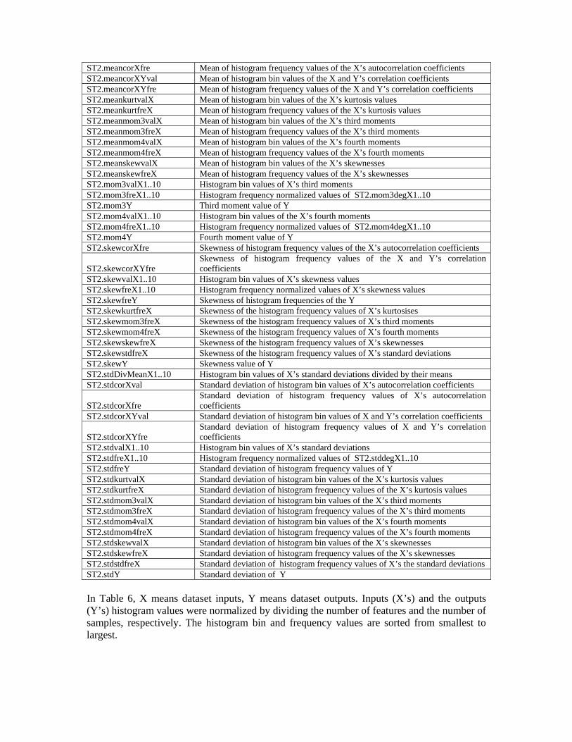
Table 6. ST2 Meta Feature Group (X:input, Y:output).

Meta Feature Name Explanation

ST2.bigcorXpro Percentage of the X’s autocorrelation coefficients bigger then 0.5 (except for diagonal)

ST2.bigcorXYpro Percentage of the X and Y’s correlation coefficients bigger then 0.5 ST2.corXval1..10 Histogram bin values of X’s autocorrelation coefficients ST2.corXfre1..10 Histogram frequency normalized values of X’s autocorrelation coefficients ST2.corXYDivstdXY1..10 Histogram bin values of the X and Y’s correlation coefficients divided by

sqrt(ST2.stdX*ST2.stdY) ST2.corXYval1..10 Histogram bin values of the X and Y’s correlation coefficients ST2.corXYfre1..10 Histogram frequency normalized values of X and Y’s correlation coefficients ST2.freY1..10 Histogram frequency normalized values of Y ST2.kurtcorXfre Kurtosis of histogram frequencies of the X’s autocorrelation coefficients ST2.kurtcorXYfre Kurtosis of histogram frequencies of the X and Y’s correlation coefficients ST2.kurtvalX1...10 Histogram bin values of X’s kurtosis values ST2.kurtfreX1..10 Histogram frequency normalized values of X’s kurtosis values ST2.kurtfreY Kurtosis of histogram frequencies of the Y ST2.kurtkurtfreX Kurtosis of the histogram frequency values of X’s kurtosises ST2.kurtmom3freX Kurtosis of the histogram frequency values of X’s third moments ST2.kurtmom4freX Kurtosis of the histogram frequency values of X’s fourth moments ST2.kurtskewfreX Kurtosis of the histogram frequency values of X’s skewnesses ST2.kurtstdfreX Kurtosis of the histogram frequency values of X’s standard deviations ST2.kurtY Kurtosis value of Y ST2.maxcorrXY Histogram’s max value of the X and Y’s correlation coefficients ST2.meancorXval Mean of histogram bin values of the X’s autocorrelation coefficients

ST2.meancorXfre Mean of histogram frequency values of the X’s autocorrelation coefficients ST2.meancorXYval Mean of histogram bin values of the X and Y’s correlation coefficients ST2.meancorXYfre Mean of histogram frequency values of the X and Y’s correlation coefficients ST2.meankurtvalX Mean of histogram bin values of the X’s kurtosis values ST2.meankurtfreX Mean of histogram frequency values of the X’s kurtosis values ST2.meanmom3valX Mean of histogram bin values of the X’s third moments ST2.meanmom3freX Mean of histogram frequency values of the X’s third moments ST2.meanmom4valX Mean of histogram bin values of the X’s fourth moments ST2.meanmom4freX Mean of histogram frequency values of the X’s fourth moments ST2.meanskewvalX Mean of histogram bin values of the X’s skewnesses ST2.meanskewfreX Mean of histogram frequency values of the X’s skewnesses ST2.mom3valX1..10 Histogram bin values of X’s third moments ST2.mom3freX1..10 Histogram frequency normalized values of ST2.mom3degX1..10 ST2.mom3Y Third moment value of Y ST2.mom4valX1..10 Histogram bin values of the X’s fourth moments ST2.mom4freX1..10 Histogram frequency normalized values of ST2.mom4degX1..10 ST2.mom4Y Fourth moment value of Y ST2.skewcorXfre Skewness of histogram frequency values of the X’s autocorrelation coefficients

ST2.skewcorXYfre Skewness of histogram frequency values of the X and Y’s correlation coefficients

ST2.skewvalX1..10 Histogram bin values of X’s skewness values ST2.skewfreX1..10 Histogram frequency normalized values of X’s skewness values ST2.skewfreY Skewness of histogram frequencies of the Y ST2.skewkurtfreX Skewness of the histogram frequency values of X’s kurtosises ST2.skewmom3freX Skewness of the histogram frequency values of X’s third moments ST2.skewmom4freX Skewness of the histogram frequency values of X’s fourth moments ST2.skewskewfreX Skewness of the histogram frequency values of X’s skewnesses ST2.skewstdfreX Skewness of the histogram frequency values of X’s standard deviations ST2.skewY Skewness value of Y ST2.stdDivMeanX1..10 Histogram bin values of X’s standard deviations divided by their means ST2.stdcorXval Standard deviation of histogram bin values of X’s autocorrelation coefficients

ST2.stdcorXfre Standard deviation of histogram frequency values of X’s autocorrelation coefficients

ST2.stdcorXYval Standard deviation of histogram bin values of X and Y’s correlation coefficients

ST2.stdcorXYfre Standard deviation of histogram frequency values of X and Y’s correlation coefficients

ST2.stdvalX1..10 Histogram bin values of X’s standard deviations ST2.stdfreX1..10 Histogram frequency normalized values of ST2.stddegX1..10 ST2.stdfreY Standard deviation of histogram frequency values of Y ST2.stdkurtvalX Standard deviation of histogram bin values of the X’s kurtosis values ST2.stdkurtfreX Standard deviation of histogram frequency values of the X’s kurtosis valuesST2.stdmom3valX Standard deviation of histogram bin values of the X’s third moments ST2.stdmom3freX Standard deviation of histogram frequency values of the X’s third moments ST2.stdmom4valX Standard deviation of histogram bin values of the X’s fourth moments ST2.stdmom4freX Standard deviation of histogram frequency values of the X’s fourth moments ST2.stdskewvalX Standard deviation of histogram bin values of the X’s skewnesses ST2.stdskewfreX Standard deviation of histogram frequency values of the X’s skewnesses ST2.stdstdfreX Standard deviation of histogram frequency values of X’s the standard deviations ST2.stdY Standard deviation of Y

In Table 6, X means dataset inputs, Y means dataset outputs. Inputs (X’s) and the outputs (Y’s) histogram values were normalized by dividing the number of features and the number of samples, respectively. The histogram bin and frequency values are sorted from smallest to largest.

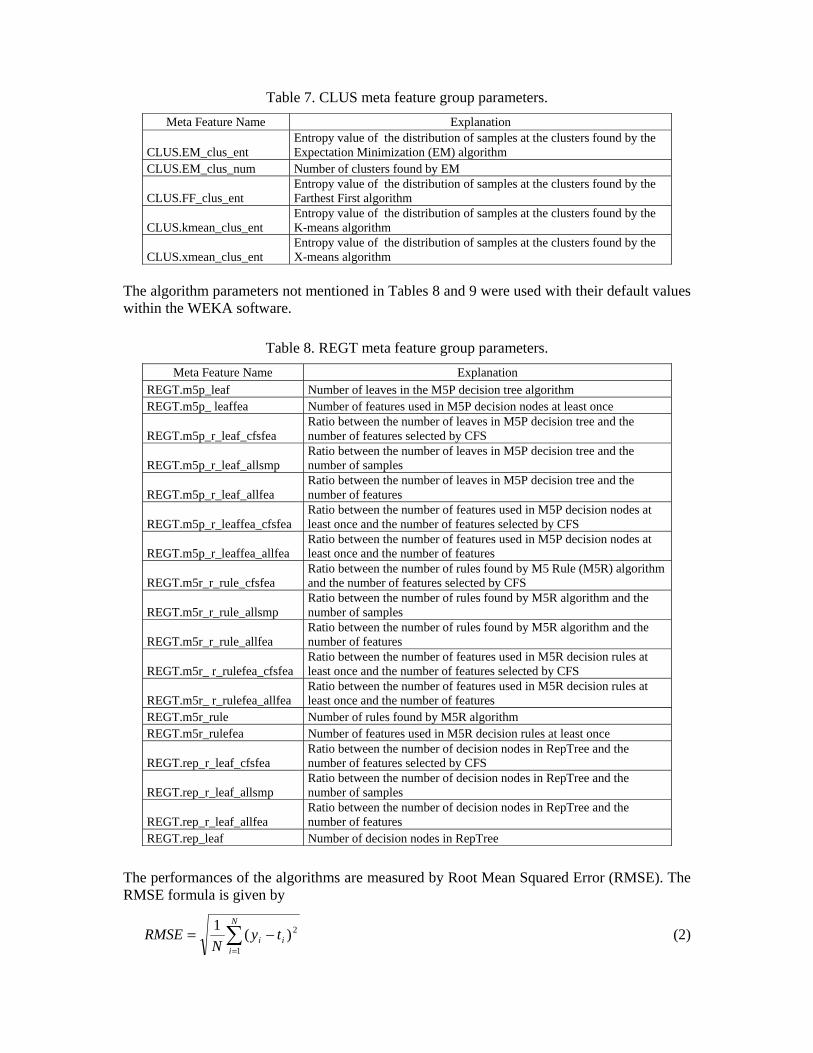
Table 7. CLUS meta feature group parameters.

Meta Feature Name Explanation

CLUS.EM_clus_ent Entropy value of the distribution of samples at the clusters found by the Expectation Minimization (EM) algorithm

CLUS.EM_clus_num Number of clusters found by EM

CLUS.FF_clus_ent Entropy value of the distribution of samples at the clusters found by the Farthest First algorithm

CLUS.kmean_clus_ent Entropy value of the distribution of samples at the clusters found by the K-means algorithm

CLUS.xmean_clus_ent Entropy value of the distribution of samples at the clusters found by the X-means algorithm

The algorithm parameters not mentioned in Tables 8 and 9 were used with their default values within the WEKA software.

Table 8. REGT meta feature group parameters.

Meta Feature Name Explanation REGT.m5p_leaf Number of leaves in the M5P decision tree algorithm REGT.m5p_ leaffea Number of features used in M5P decision nodes at least once

REGT.m5p_r_leaf_cfsfea Ratio between the number of leaves in M5P decision tree and the number of features selected by CFS

REGT.m5p_r_leaf_allsmp Ratio between the number of leaves in M5P decision tree and the number of samples

REGT.m5p_r_leaf_allfea Ratio between the number of leaves in M5P decision tree and the number of features

REGT.m5p_r_leaffea_cfsfea Ratio between the number of features used in M5P decision nodes at least once and the number of features selected by CFS

REGT.m5p_r_leaffea_allfea Ratio between the number of features used in M5P decision nodes at least once and the number of features

REGT.m5r_r_rule_cfsfea Ratio between the number of rules found by M5 Rule (M5R) algorithm and the number of features selected by CFS

REGT.m5r_r_rule_allsmp Ratio between the number of rules found by M5R algorithm and the number of samples

REGT.m5r_r_rule_allfea Ratio between the number of rules found by M5R algorithm and the number of features

REGT.m5r_ r_rulefea_cfsfea Ratio between the number of features used in M5R decision rules at least once and the number of features selected by CFS

REGT.m5r_ r_rulefea_allfea Ratio between the number of features used in M5R decision rules at least once and the number of features

REGT.m5r_rule Number of rules found by M5R algorithm REGT.m5r_rulefea Number of features used in M5R decision rules at least once

REGT.rep_r_leaf_cfsfea Ratio between the number of decision nodes in RepTree and the number of features selected by CFS

REGT.rep_r_leaf_allsmp Ratio between the number of decision nodes in RepTree and the number of samples

REGT.rep_r_leaf_allfea Ratio between the number of decision nodes in RepTree and the number of features

REGT.rep_leaf Number of decision nodes in RepTree

The performances of the algorithms are measured by Root Mean Squared Error (RMSE). The RMSE formula is given by

=

−=N

iii ty

NRMSE

1

2)(1

(2)

where iy and it define the target value and the estimated value of the ith sample,

respectively. N is the number of samples.

Table 9. RMSE (landmarks) Meta Feature Group (The RMSE values of the algorithms).

Meta Feature Name

Description and Reference

RMSE.M5R M5 rules and M5P algorithms (Wang et all., 1997) RMSE.M5P

RMSE. Decstump (DecS)

Decision Stump: Generates only one decision node and two leaves. The decision node consists of only one feature and a threshold value. The selection of these parameters is based on minimizing Mean Squared Error (MSE).

RMSE.PLS2 Partial Least Squares Algorithm (Abdi, 2003) The numbers after the algorithm names define the number of components used in the PLS algorithm. RMSE.PLS1

RMSE.SLR Simple Linear Regression: Construct linear models for each feature. The model having minimum MSE is selected.

RMSE.SMO Sequential minimal optimization and Support vector machine algorithms (Shevade et all., 1999) RMSE.SVM

RMSE.IBK One Nearest Neighbor Algorithm (Aha et all., 1991) RMSE.ZeroR (default error)

Zero Rule: The algorithm simply predicts the average of outputs of training data for all test samples.

RMSE.ConjunctiveRule (ConR)

ConjunctiveRule algorithm: Generates only one rule consisting of several feature — threshold pairs.

RMSE.LinearRegression (LR)

LinearRegression: Constructs one linear model consisting of all features.

RMSE. RBF Radial Basis Functions: First, selects the cluster means by Kmeans algorithm, and then fits radial basis functions for each cluster mean.

RMSE.Kstar Kstar Algorithm (Cleary et all., 1995) RMSE.LWL Locally weighted learning algorithm (Frank et all., 2003)

If an algorithm’s performance is satisfactory on a dataset, it can be said that the dataset can be handled by the applied algorithm. For example, the success of a linear based algorithm can be seen as the measure of linearity of that dataset. Similarly, the success of a successful Bayes algorithm on a dataset means the independence of features of that dataset (Bensusan et all., 2000a).

Table 10. PCA meta feature group parameters.

Meta Feature Name ExplanationPCA.expval1..10 Histogram bin values of the proportion of variance explained by each principal

component PCA.expfre1..10 Histogram frequency normalized values of PCA.expval1.10 PCA.explained_1 Proportion of variance explained by the first principal component

PCA.x95 Ratio between the number of principle components which explains 95% of variance and the number of features

4.2 Extra Meta Features in Addition to Standard Features In some dataset collections, there are some other meta features added to the standard ones. In the drug dataset collection, the problem type (biological activity, melting point etc.) is known. In Friedman collection, colinearity is known. However, some learning algorithms could not be

successfully applied on all the datasets because of time and memory restrictions. Cosequently, the performances of some algorithms are given in terms of the extra meta features. For Friedman Collection, there are 15 extra meta features. They are shown in Table 11. The basic descriptions of a meta algorithm is given next to the name of the meta algorithm.

Table 11. The extra meta features used in the Friedman collection.

Meta Feature Name Description and Reference Colli Colinearity degree {0,1,2,3,4} — for details, see Section 3.1. RMSE.GaussianProcesses (GausP)

Implements gaussian processes for regression without hyperparameter-tuning. (Mackay, 1998)

RMSE.meta.AdditiveRegression (Decision Stump) (mt.AR)

(Friedman, 1999)

RMSE.meta.AttributeSelectedClassifier (M5P) (mt.AS)

Dimensionality of training and test data is reduced by attribute selection before being passed on to a classifier.

RMSE.meta.Bagging (RepTree) (mt.Bag)

(Breiman, 1996)

RMSE.meta.Dagging (IBK) (mt.Dag)

(Ting and Witten, 1997)

RMSE.meta.EnsembleSelc. (SmoReg – m5rules – ZeroR) (mt.ES)

(Caruana et al,2004)

RMSE.meta.RandomSubSpace (RepTree) (mt.RS)

(Ho, 1998)

RMSE.meta.RegressionByDiscretization (C4.5) (mt.RD)

A regression scheme that employs any classifier on a copy of the data that has the class attribute (equal-width) discretized. The predicted value is the expected value of the mean class value for each discretized interval (based on the predicted probabilities for each interval).

RMSE.meta.Stacking (SmoReg – m5rules – ZeroR) (mt.St)

(Wolpert, 1992)

RMSE.meta.Vote (SmoReg – m5rules – ZeroR) (mt.Vo)

(Kuncheva, 2004)

RMSE.REPTree (RepT) Builds a decision/regression tree using information gain/variance and prunes it using reduced-error pruning (with backfitting).

RMSE.PLS3 Partial Least Squares Algorithm (Abdi, 2003) The numbers after the algorithm names define the number of components used in PLS algorithm. RMSE.PLS4

RMSE.PLS5

The extra meta features used in the Drug Collection are given in Table 12.

Table 12. The extra meta features used in the Drug Collection.

Meta Feature Name Explanation

Prob_type Problem type : a=Biological activity, m=Melting point, d=other. For details, see Table 2.

RMSE.PLS3 See Table 11.

RMSE.PLS4 RMSE.PLS5 RMSE.REPTree See Table 11.

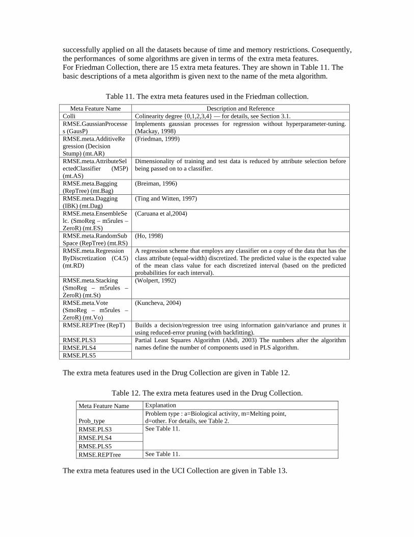
The extra meta features used in the UCI Collection are given in Table 13.

Table 13. The extra meta features used in the UCI Collection.

Meta Feature Name Description and Reference

RMSE.isotonicreg (ISO) Learns an isotonic regression model. Picks the attribute that result in the lowest squared error.

RMSE.leastmedsq (LMS)

(Rousseeuw and Leroy, 1987)

RMSE.MLP The common multilayer perceptron architecture with the backpropogation algorithm.

4.3 Working with Samples Having Different Dimensionalities The dimensionality of each sample (dataset) in the meta space can be different if some meta features (kurtosis, standard deviation etc.) are calculated for each feature of a dataset. This form of meta dataset is a problem for common approaches/algorithms. Such a meta dataset needs an aggregation function. In the literature, different kinds of functions are used for this purpose. The simple ones are average, minimum and maximum feature vectors. Some researchers use histograms for fine grained aggregation of the individual attributes (Kalousis and Theoharis, 1999). Histograms preserve more information about meta features compared to the simple aggregation functions. In our study, the histogram’s bin and frequency values, and the shape of histograms were used. The bin number is 10 for all histograms. 5. Experimental Results In this section, the meta regression studies on 3 different dataset collections are given. The experiments and analyses below were done for each dataset collection, and consists of

• Analysis of algorithm performances over datasets • Correlation analysis of meta features • The hierarchical clustering of algorithms and datasets according to the performances

of the algorithms • The prediction of performances of successful algorithms with meta features • Analysis of meta features used in the performance prediction of algorithms.

5.1 Performances of Algorithms The algorithms were tested on each dataset in each dataset collection. The RMSE values were calculated using 10-fold cross validation. In Table 14, the mean RMSE values (MRMSE) and the mean standard deviations of the RMSE values (MSTD) measured with each algorithm over 3 dataset collections are given. The number next to Mean RMSE (MRMSE) means how many times the algorithm has the minimum RMSE in the collection. For example, the M5P algorithm is the best algorithm 21 times in 60 UCI datasets, 4 times in 41 Drug datasets and 18 times in 80 Friedman datasets. Table 14. The mean RMSE values and the mean standard deviations of the algorithms measured with the dataset collections (NA means “not applied”).

Algorithm Names UCI_MRMSE(60 datasets)

DRG_MRMSE(41 datasets)

FRI_MRMSE (80 datasets) UCI_MSTD DRG_MSTD FRI_MSTD

Conjunctive rules 0,1548 (1) 0,245 0,8735 0,0668 0,084 0,0616

Decstump 0,1547 0,256 (2) 0,869 0,0644 0,099 0,0604 IBK 0,1477 (1) 0,244 (2) 1,0091 0,0877 0,128 0,2775 Kstar 0,1345 (4) 0,222 (12) 0,889 (4) 0,0797 0,096 0,27

Linear Regression 0,1448 (4) 1922,91 0,8618 (1) 0,1275 1006,39 0,4669

LWL 0,1435 (2) 0,2611 0,8134 0,0606 0,103 0,0531

M5P 0,1062 (21) 0,239 (4) 0,5055 (18) 0,0692 0,11 0,1212 M5R 0,1087 (3) 0,247 (1) 0,5401 0,0691 0,097 0,12 PLS1 0,1427 (4) 0,223 (2) 0,8361 0,06 0,091 0,1302

PLS2 0,1308 (2) 0,226 (3) 0,8284 0,0617 0,111 0,1438 RBF 0,173 0,257 0,9342 0,0676 0,088 0,0625 SLR 0,144 0,313 (5) 0,8834 0,0683 0,305 0,042

SMO 0,1656 (6) 24,21 (1) 0,8982 0,3415 0,611 0,2706 SVM 0,1655 (1) 24,17 0,8981 0,3414 0,61 0,2706 Zero Rule 0,1948 (2) 0,25 0,9949 0,0775 0,0075 0,0069

REPTree NA 0,256 (1) 0,6236 NA 0,096 0,1289 Gaussian Processes NA NA 0,8056 (7) NA NA 0,1801 meta.AdditiveRegression NA NA 0,5514 (8) NA NA 0,0746

meta.AttributeSelectedClassifier NA NA 0,6001 (9) NA NA 0,122 meta.Bagging NA NA 0,5009 (33) NA NA 0,1241 meta.Dagging NA NA 0,8012 NA NA 0,1655

meta.EnsembleSelection NA NA 0,7073 NA NA 0,1241 meta.RandomSubSpace NA NA 0,6168 NA NA 0,0987 meta.RegressionByDiscretization NA NA 0,6413 NA NA 0,1409

meta.Stacking NA NA 0,9941 NA NA 0,0056 meta.Vote NA NA 0,7115 NA NA 0,0947 PLS3 NA 0,239 (1) 0,8369 NA 0,13 0,1581

PLS4 NA 0,231 (2) 0,8405 NA 0,128 0,1701 PLS5 NA 0,245 (5) 0,8444 NA 0,144 0,1823 isotonic regression 0,1383 (3) NA NA 0,07 NA NA Leastmedsq 0,1567 (1) NA NA 0,0987 NA NA MLP 0,1585 (5) NA NA 0,1679 NA NA

According to FRI_MRMSE and FRI_MSTD columns of Table 14, the component number in the PLS algorithm does not affect performance. The algorithms having the maximum standard deviations are LinearRegression, IBK, SMOreg, SVMreg, and Kstar, respectively. According to DRG_MRMSE column of Table 14, Linear Regression, SVMreg and SMOreg algorithms did not converge on some drug datasets. According to UCI_MSTD column of Table 14, the algorithms having the maximum standard deviations are SMOreg, SVMreg, MLP, Linear Regression, respectively. 5.2 The Correlation of Meta Features In this section, the correlations between the meta features are analyzed for each dataset collection. The highly correlated meta feature pairs guide the meta learning dynamics. There are 310, 300 and 298 meta features in Friedman, Drug and UCI collections, respectively. The correlation coefficient of each meta feature pairs is calculated in each collection. The meta feature pairs are considered as correlated if the correlation coefficient’s absolute values are bigger than 0.8. The number of correlated meta feature pairs are 1707, 853 and 655, respectively, in the dataset collections Friedman, Drug and UCI. The highly correlated pairs out of all pair ratios are 3.5 %, 1.9% and 1.5%, respectively. In Tables 15, 16 and 17, the number of correlated meta features are given with respect to meta feature groups in each dataset collection.

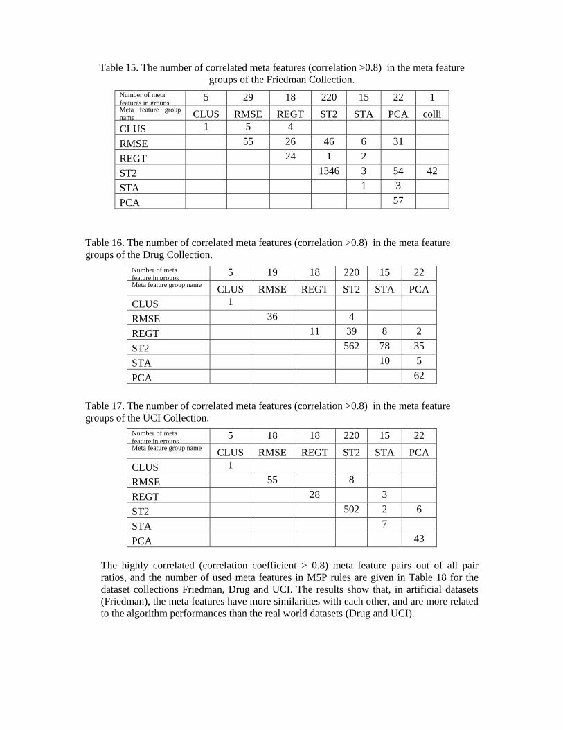
Table 15. The number of correlated meta features (correlation >0.8) in the meta feature groups of the Friedman Collection.

Number of meta features in groups

5 29 18 220 15 22 1 Meta feature group name CLUS RMSE REGT ST2 STA PCA colli

CLUS 1 5 4

RMSE 55 26 46 6 31

REGT 24 1 2

ST2 1346 3 54 42

STA 1 3

PCA 57

Table 16. The number of correlated meta features (correlation >0.8) in the meta feature groups of the Drug Collection.

Number of meta feature in groups

5 19 18 220 15 22 Meta feature group name CLUS RMSE REGT ST2 STA PCA

CLUS 1

RMSE 36 4

REGT 11 39 8 2

ST2 562 78 35

STA 10 5

PCA 62

Table 17. The number of correlated meta features (correlation >0.8) in the meta feature groups of the UCI Collection.

Number of meta feature in groups

5 18 18 220 15 22 Meta feature group name CLUS RMSE REGT ST2 STA PCA

CLUS 1

RMSE 55 8

REGT 28 3

ST2 502 2 6

STA 7

PCA 43

The highly correlated (correlation coefficient > 0.8) meta feature pairs out of all pair ratios, and the number of used meta features in M5P rules are given in Table 18 for the dataset collections Friedman, Drug and UCI. The results show that, in artificial datasets (Friedman), the meta features have more similarities with each other, and are more related to the algorithm performances than the real world datasets (Drug and UCI).

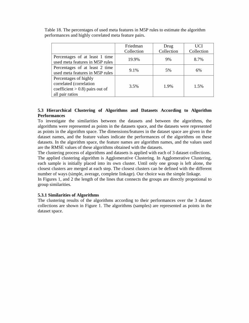
Table 18. The percentages of used meta features in M5P rules to estimate the algorithm performances and highly correlated meta feature pairs.

Friedman

Collection Drug

Collection UCI

Collection Percentages of at least 1 time used meta features in M5P rules

19.9% 9% 8.7%

Percentages of at least 2 time used meta features in M5P rules

9.1% 5% 6%

Percentages of highly correlated (correlation coefficient > 0.8) pairs out of all pair ratios

3.5% 1.9% 1.5%

5.3 Hierarchical Clustering of Algorithms and Datasets According to Algorithm Performances To investigate the similarities between the datasets and between the algorithms, the algorithms were represented as points in the datasets space, and the datasets were represented as points in the algorithm space. The dimensions/features in the dataset space are given in the dataset names, and the feature values indicate the performances of the algorithms on these datasets. In the algorithm space, the feature names are algorithm names, and the values used are the RMSE values of these algorithms obtained with the datasets. The clustering process of algorithms and datasets is applied with each of 3 dataset collections. The applied clustering algorithm is Agglomerative Clustering. In Agglomerative Clustering, each sample is initially placed into its own cluster. Until only one group is left alone, the closest clusters are merged at each step. The closest clusters can be defined with the different number of ways (simple, average, complete linkage). Our choice was the simple linkage. In Figures 1, and 2 the length of the lines that connects the groups are directly propotional to group similarities. 5.3.1 Similarities of Algorithms The clustering results of the algorithms according to their performances over the 3 dataset collections are shown in Figure 1. The algorithms (samples) are represented as points in the dataset space.

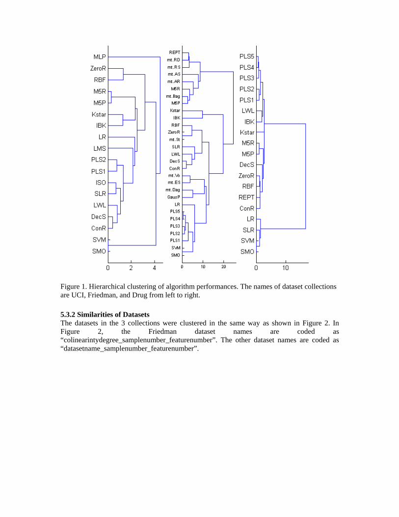
Figure 1. Hierarchical clustering of algorithm performances. The names of dataset collections are UCI, Friedman, and Drug from left to right.

5.3.2 Similarities of Datasets The datasets in the 3 collections were clustered in the same way as shown in Figure 2. In Figure 2, the Friedman dataset names are coded as “colinearintydegree_samplenumber_featurenumber”. The other dataset names are coded as “datasetname_samplenumber_featurenumber”.

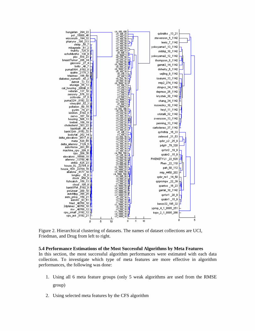
Figure 2. Hierarchical clustering of datasets. The names of dataset collections are UCI, Friedman, and Drug from left to right.

5.4 Performance Estimations of the Most Successful Algorithms by Meta Features In this section, the most successful algorithm performances were estimated with each data collection. To investigate which type of meta features are more effective in algorithm performances, the following was done:

1. Using all 6 meta feature groups (only 5 weak algorithms are used from the RMSE

group)

2. Using selected meta features by the CFS algorithm

The algorithm performance estimations were done by using two groups of meta features described above. 10-fold cross validation was used in all the experiments. The 10-fold performance values were averaged and reported. In all the estimation experiments, the M5P algorithm is used because of its high performance. This algorithm also produces useful rules including used meta features and their weights on performance estimation. By these rules, the performance estimations can be easily interpreted. The Relative Absolute Error (RAE) and Correlation Coefficient (CC) are used instead of RMSE for evaluation of performance estimation because their output ranges are very different from each other. RAE is calculated by

=

=

−

−=

N

ii

N

iii

yy

tyRAE

1

*

1 (2)

where *y : The average of the actual target values of the samples

*t : The average of the estimated values of the samples The algoritms used to estimate the performances of other algorithms with all 3 dataset collections were Decision Stump, Linear Regression, ZeroR. RBF was used in the Drug and UCI collections. IBK was used in the Friedman and UCI collections. SLR was used in the Friedman collection. RepTree was used in the Drug collection. The performance estimation experimental results are given in Tables 19, 20, and 21 with RAE and Correlation coefficients. Each algorithm performance was estimated with two groups of meta features.

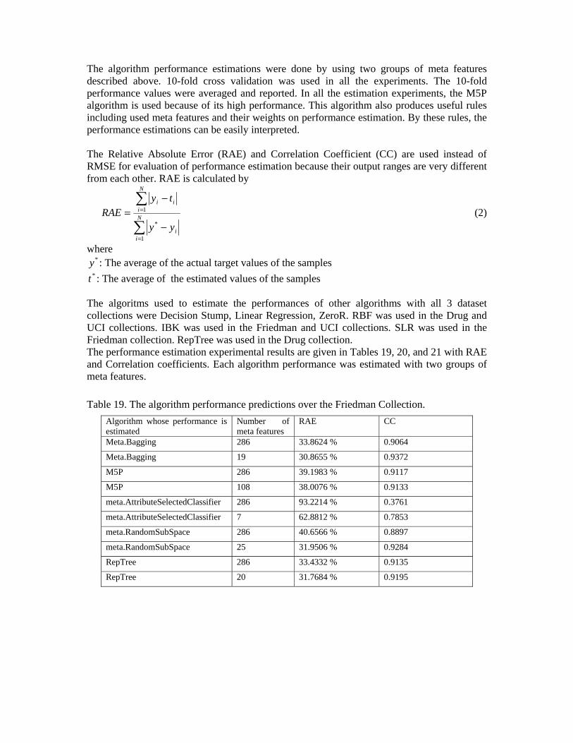
Table 19. The algorithm performance predictions over the Friedman Collection.

Algorithm whose performance is estimated

Number of meta features

RAE CC

Meta.Bagging 286 33.8624 % 0.9064

Meta.Bagging 19 30.8655 % 0.9372

M5P 286 39.1983 % 0.9117

M5P 108 38.0076 % 0.9133

meta.AttributeSelectedClassifier 286 93.2214 % 0.3761

meta.AttributeSelectedClassifier 7 62.8812 % 0.7853

meta.RandomSubSpace 286 40.6566 % 0.8897

meta.RandomSubSpace 25 31.9506 % 0.9284

RepTree 286 33.4332 % 0.9135

RepTree 20 31.7684 % 0.9195

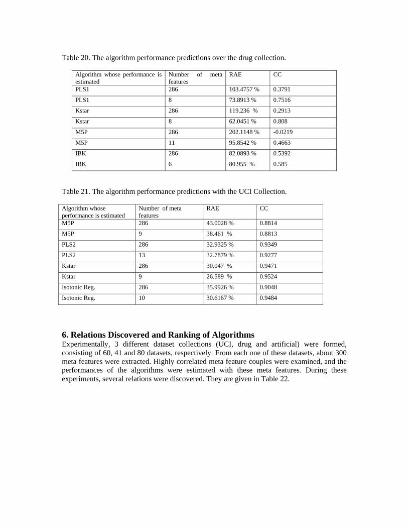
Table 20. The algorithm performance predictions over the drug collection.

Algorithm whose performance is estimated

Number of meta features

RAE CC

PLS1 286 103.4757 % 0.3791

PLS1 8 73.8913 % 0.7516

Kstar 286 119.236 % 0.2913

Kstar 8 62.0451 % 0.808

M5P 286 202.1148 % -0.0219

M5P 11 95.8542 % 0.4663

IBK 286 82.0893 % 0.5392

IBK 6 80.955 % 0.585

Table 21. The algorithm performance predictions with the UCI Collection. Algorithm whose performance is estimated

Number of meta features

RAE CC

M5P 286 43.0028 % 0.8814

M5P 9 38.461 % 0.8813

PLS2 286 32.9325 % 0.9349

PLS2 13 32.7879 % 0.9277

Kstar 286 30.047 % 0.9471

Kstar 9 26.589 % 0.9524

Isotonic Reg. 286 35.9926 % 0.9048

Isotonic Reg. 10 30.6167 % 0.9484

6. Relations Discovered and Ranking of Algorithms Experimentally, 3 different dataset collections (UCI, drug and artificial) were formed, consisting of 60, 41 and 80 datasets, respectively. From each one of these datasets, about 300 meta features were extracted. Highly correlated meta feature couples were examined, and the performances of the algorithms were estimated with these meta features. During these experiments, several relations were discovered. They are given in Table 22.

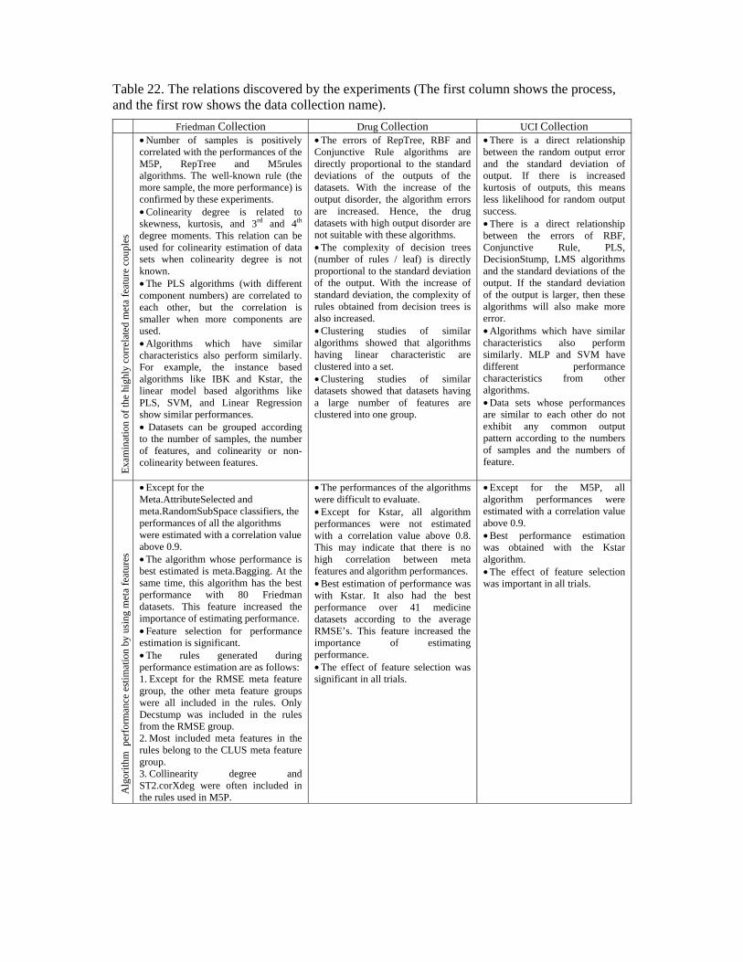
Table 22. The relations discovered by the experiments (The first column shows the process, and the first row shows the data collection name).

Friedman Collection Drug Collection UCI Collection E

xam

inat

ion

of th

e hi

ghly

cor

rela

ted

met

a fe

atur

e co

uple

s

• Number of samples is positively correlated with the performances of the M5P, RepTree and M5rules algorithms. The well-known rule (the more sample, the more performance) is confirmed by these experiments. • Colinearity degree is related to skewness, kurtosis, and 3rd and 4th degree moments. This relation can be used for colinearity estimation of data sets when colinearity degree is not known. • The PLS algorithms (with different component numbers) are correlated to each other, but the correlation is smaller when more components are used. • Algorithms which have similar characteristics also perform similarly. For example, the instance based algorithms like IBK and Kstar, the linear model based algorithms like PLS, SVM, and Linear Regression show similar performances. • Datasets can be grouped according to the number of samples, the number of features, and colinearity or non-colinearity between features.

• The errors of RepTree, RBF and Conjunctive Rule algorithms are directly proportional to the standard deviations of the outputs of the datasets. With the increase of the output disorder, the algorithm errors are increased. Hence, the drug datasets with high output disorder are not suitable with these algorithms. • The complexity of decision trees (number of rules / leaf) is directly proportional to the standard deviation of the output. With the increase of standard deviation, the complexity of rules obtained from decision trees is also increased. • Clustering studies of similar algorithms showed that algorithms having linear characteristic are clustered into a set. • Clustering studies of similar datasets showed that datasets having a large number of features are clustered into one group.

• There is a direct relationship between the random output error and the standard deviation of output. If there is increased kurtosis of outputs, this means less likelihood for random output success. • There is a direct relationship between the errors of RBF, Conjunctive Rule, PLS, DecisionStump, LMS algorithms and the standard deviations of the output. If the standard deviation of the output is larger, then these algorithms will also make more error. • Algorithms which have similar characteristics also perform similarly. MLP and SVM have different performance characteristics from other algorithms. • Data sets whose performances are similar to each other do not exhibit any common output pattern according to the numbers of samples and the numbers of feature.

Alg

orith

m p

erfo

rman

ce e

stim

atio

n by

usi

ng m

eta

feat

ures

• Except for the Meta.AttributeSelected and meta.RandomSubSpace classifiers, the performances of all the algorithms were estimated with a correlation value above 0.9. • The algorithm whose performance is best estimated is meta.Bagging. At the same time, this algorithm has the best performance with 80 Friedman datasets. This feature increased the importance of estimating performance. • Feature selection for performance estimation is significant. • The rules generated during performance estimation are as follows: 1. Except for the RMSE meta feature group, the other meta feature groups were all included in the rules. Only Decstump was included in the rules from the RMSE group. 2. Most included meta features in the rules belong to the CLUS meta feature group. 3. Collinearity degree and ST2.corXdeg were often included in the rules used in M5P.

• The performances of the algorithms were difficult to evaluate. • Except for Kstar, all algorithm performances were not estimated with a correlation value above 0.8. This may indicate that there is no high correlation between meta features and algorithm performances. • Best estimation of performance was with Kstar. It also had the best performance over 41 medicine datasets according to the average RMSE’s. This feature increased the importance of estimating performance. • The effect of feature selection was significant in all trials.

• Except for the M5P, all algorithm performances were estimated with a correlation value above 0.9. • Best performance estimation was obtained with the Kstar algorithm. • The effect of feature selection was important in all trials.

Sim

ilari

ties

of A

lgor

ithm

s

• Linear based algorithms were clustered together. • The single rule algorithms Conjunctive Rule and Decision Stump were clustered together. • Sample based algorithms Kstar and IBK were clustered together. • Decision Trees and Meta Algorithms M5P, M5R, RepTree, meta.Bagging, meta.Attribute selected, meta.Additive Regresson, meta.Random Subspace and meta.Regression byDiscrization were clustered together. This is because such meta algorithms generally use decision tree algorithms as base algorithms.

• Linear based algorithms were clustered together. • PLS family algorithms were clustered together. • Algorithms are divided into two clusters which were very distant from each other.

• The one-rule generating algorithms Conjunctive Rule and Decision Stump were clustered together. • Sample based algorithms Kstar and IBK were clustered together. • The PLS algorithms having different dimension numbers were clustered together. • MLP and SVM showed very different performance characteristics as compared to other algorithms.

Sim

ilar

itie

s of

Dat

aset

s

• The datasets were clustered into several groups. These dataset groups can be defined as • Including 100 samples • Including more than 500 samples • Having 5 features • Having 10 features • Having colinearity values equal to 0 With these results, it can be said that the datasets were clustered according to their number of features, number of samples and colinearity values.

Datasets having 1142 features were clustered together.

The groups had no common similarity patterns according to their number of features and number of samples.

The success rankings of algorithms are summarized in Table 23. The explanation of Average of Zero rule RMSE is given in Table 9.

Table 23. The success ranking of algorithms over 3 data collections

Average of Zero rule RMSE (default error)

The best performed algorithm and its average RMSE

The success ranking of the best algorithms(according to average RMSEs)

Friedman Collection (80 datasets)

0.995 Meta.Bagging 0.501

Meta.Bagging > M5P > M5rules > meta.AttrSelClas > meta.RandomSubSpace > RepTree

Drug Collection (41 datasets)

0.25 Kstar 0.222

Kstar > PLS1 > PLS2 > PLS4 > PLS3 > M5P > IBK > PLS5 > Conjunctive Rule

UCI Collection (60 datasets)

0.195 M5P 0.106

M5P > M5R > PLS2 > Kstar > Isotonic Reg. > PLS1

7. Summary and Conclusions With all the data sets, there is no single algorithm that always gives better results than the other algorithms. For this reason, which algorithm works best with a given dataset is usually determined by trial and error. To reduce this deficiency and to form an auxiliary series of rules for non-expert users, some approaches were developed in the literature, the aim being the estimation of the performances of a pool of algorithms by using various features of a dataset. This approach is called Meta-Learning. The current meta-learning studies have generally been carried out with classification data. Regression data is also very important in

machine learning. In this study, we have investigated the dynamics between meta features and algorithm performances with regression data. In our study, the standard and newly proposed dataset features were used as meta features. Some models were developed to estimate the potential performances of algorithms over given datasets. We also studied clustering the datasets and the algorithms with respect to their similarity between each other in RMSE spaces, respectively. The results with the 3 data collections also indicate the following findings:

• According to the Zero rule, the datasets having maximum average RMSE’s are the artificial (Friedman) datasets.

• The diagonal values are very big in Tables 15, 16, and 17. This proves that the meta features within the same groups are more correlated with each other. Especially, the meta features in the ST2 group are highly correlated with each other.

• The most successful algorithm usually changes with each individual data collection. • The drug collection datasets are the most difficult ones since the algorithms cannot

reduce the errors much beyond random error (zero rule error). • The M5P algorithm is among the best performing algorithms with all the dataset

collections. • If the RMSE of an algorithm is big with a data set, estimating the RMSE of the

algorithm becomes difficult. Estimating the the RMSE of successful algorithms is rather easy.

• The meta features most used in the estimation of the performances of the algorithms over all the 3 dataset collections are listed below. These meta features can be considered to be the features of the datasets most related to the performances of the algorithms.

• RMSE value of Decstump algorithm • The proportion between the number of samples and the number of rules

discovered with M5rules (REGT group) • The number of features used at least once in the leaves of the M5P decision

tree (REGT group) • The proportion of the number of samples and the number of leaves with the

M5P decision tree (REGT group) • The proportion of the number of features and the number of features used at

least once in the leaves of the M5P decision tree (REGT group) • The number of selected features by the CFS algorithm (STA group) • The number of samples (STA group)

The meta datasets used can be downloaded from http://dynamo.ecn.purdue.edu/~ersoy/metadata. These datasets may be useful to interested meta learning researchers.

References

J. Fürnkranz and J. Petrak, (2001), “An evaluation of landmarking variants”, Proceedings of the ECML/PKDD Workshop on Integrating Aspects of Data Mining, Decision Support and Meta-Learning.

Bensusan H., C. Giraud-Carrier, C. J. Kennedy, (2000b), “A Higher-order Approach to Meta-Learning”, Proceedings of the Work-in-Progress Track at the 10th International Conference on Inductive Logic Programming.

Kalousis, A. Ve Hilario, M., (2000), “Model Selection via Meta-learning: a Comparative Study”, Tools with Artificial Intelligence-ICTAI. Proceedings. 12th IEEE International Conference.

Kalousis, A. Ve Hilario, M., (2003), “Representational Issues in Meta-Learning”, In Proceedings of the 20th International Conference on Machine Learning –ICML.

Carrier, C. G., (2005), “The Data Mining Advisor: Meta-learning at the Service of Practitioners”, In Proceedings of the 4th International Conference on Machine Learning Applications, 113-119.

Todorovski L., H. Blockeel ve S. Dzeroski, (2002a), “Ranking with predictive clustering trees”, In Proceedings of the 13th European Conference on Machine Learning, volume 2430 of Lecture Notes in Artificial Intelligence, pages 444-455. SpringerVerlag.

Todorovski L. Ve S. Dzeroski, (1999), “Experiments in meta-level learning with ILP”, Proceedings of third European Conference on Principles of data mining and knowledge discovery –PKDD.

Gama J. Ve P. Brazdil, (1995), “Characterization of Classification Algorithms”, 7th Portuguese Conference on Artificial Intelligence-EPIA.

Todorovski L., P. Brazdil ve C. Soares, (2002b), “Experiments with Automatic Feature Selection in Meta-Learning”, Technical Report Jozef Stefan Instute.

Peng, P. Y., A. Flach, P. Brazdil ve C. Soares, (2002), “Decision tree-based characterization for meta-learning”, ECML/PKDD’02 workshop on Integration and Collaboration Aspects of Data Mining, Decision Support and Meta-Learning.

Brazdil P.B., Soares C. Ve Costa J.P, (2003), “Ranking Learning Algorithms: Using IBL and Meta-Learning on Accuracy and Time Results”, Machine Learning, Volume 50, Number 3, pp. 251-277(27).

Bensusan H. Ve A. Kalousis, (2001), “Estimating the Predictive Accuracy of a Classifier”, Proceedings of the 12th European Conference on Machine Learning, pp. 25-36.

Ali, S. Ve Smith, K. A., (2006), “On Learning Algorithm Selection for Classification” Applied Soft Computing, Elsevier Science, vol.6(2), pp.119-138.

C. Soares, P. B. Brazdil, P. Kuba, .A Meta-Learning Method to Select the KernelWidth in Support Vector Regression. Machine Learning, 54, 195–209, 2004

M. Pechenizkiy: Data Mining Strategy Selection via Empirical and Constructive Induction. Databases and Applications 2005: 59-64

J.H. Friedman. Greedy function approximation: A gradient boosting machine. Annals of Statistics,29,1189—1232,2001.

B. D. Silverman and Daniel. E. Platt, J. Med. Chem. 1996, 39, 2129-2140

Bergstrom, C. A. S.; Norinder, U.; Luthman, K.; Artursson, P. , Molecular Descriptors Influencing Melting Point and Their Role in Classification of Solid Drugs. J. Chem. Inf. Comput. Sci.; (Article); 2003; 43(4); 1177-1185

D. E Patterson, Richard D Cramer, Allan M Ferguson, Robert D Clark, Laurence W Weinberger. Neighbourhood Behaviour: A Useful Concept for Validation of "Molecular Diversity" Descriptors. J. Med. Chem. 1996 (39) 3049 - 3059.

Karthikeyan, M.; Glen, R.C.; Bender, A. General melting point prediction based on a diverse compound dataset and artificial neural networks. J. Chem. Inf. Model.; 2005; 45(3); 581-590

Harrison,P.W. and Barlin,G.B. and Davies,L.P. and Ireland,S.J. and Matyus,P. and Wong,M.G., Syntheses, pharmacological evaluation and molecular modelling of substituted 6-alkoxyimidazo[1,2-b]pyridazines as new ligands for the benzodiazepine receptor, European Journal of Medicinal Chemistry, (31), 1996, 651-662

H. Kubinyi. "QSAR: Hansch Analysis and Related Approaches", VCH, Weinhein (Ger), 1993, pp.57-68

Todeschini, R.; Gramatica, P.; Marengo, E.; Provenzani, R. Weighted Holistic Invariant Molecular Descriptors. Part 2. Theory Development and Applications on Modeling Physico-Chemical Properties of PolyAromatic Hydrocarbons (PAH). Chemom. Intell. Lab. Syst. 1995, 27, 221-229.

R. Guha and P. Jurs. The Development of Linear, Ensemble and Non-linear Models for the Prediction and Interpretation of the Biological Activity of a Set of PDGFR Inhibitors. J. Chem. Inf. Comput. Sci. 2004, 44 (6), 2179-2189

Cammarata, A. Interrelationship of the Regression Models Used for Structure-Activity Analyses. J. Med. Chem. 1972, 15, 573-577

Jun Feng, Predictive Toxicology: Benchmarking Molecular Descriptors and Statistical Methods, J. Chem. Inf Comput. Sci., 2003 (43) 1463-1470

Damborsky, J., Schultz, T.W., Comparison of the QSAR models for toxicity and biodegradability of anilines and phenols, Chemosphere 34: 429-446, 1997a

Blaha, L., Damborsky, J., Nemec, M., QSAR for acute toxicity of saturated and unsaturated halogenated aliphatic compounds, Chemosphere 36: 1345-1365, 1998

Damborsky, J. et al., Structure-biodegradability relationships for chlorinated dibenzo-p-dioxins and dibenzofurans, In: Wittich, R.-M., Biodegradation of dioxins and furans, R.G. Landes Company, Austin, 1998a

Damborsky, J. et al., A mechanistic approach to deriving QSBR- A case study: dehalogenation of haloaliphatic compounds, In: Peijnenburg, W.J.G.M., Damborsky, J., Biodegradability Prediction, Kluwer Academic Publishers,1998b

Damborsky, J. et al., Mechanism-based Quantitative Structure-Biodegradability Relationships for hydrolytic dehalogenation of chloro- and bromo-alkenes, Quantitative Structure-Activity Relationships 17: 450-458, 1998c

Damborsky, J., Quantitative structure-function relationships of the single-point mutants of haloalkane dehalogenase: A multivariate approach, Qunatitative Structure-Activity Relationships 16: 126-135, 1997b

Damborsky, J., Quantitative structure-function and structure-stability relationships of purposely modified proteins, Protein Engineering 11: 21-30, 1998d

Cajan, M. et al., Stability of Aromatic Amides with Bromide Anion: Quantitative Structure-Property Relationships, Journal of Chemical Information and Computer Sciences, in press, 2000

Selwood, D. L.; Livingstone, D. J.; Comley, J. C.; O'Dowd, A. B.; Hudson, A. T.; Jackson, P.; Jandu, K. S.; Rose, V. S.; Stables, J. N. Structure-Activity Relationships of Antifilarial Antimycin Analogues: A Multivariate Pattern Recognition Study J. Med. Chem., 1990, 33, 136-142

M. A. Hall (1998). Correlation-based Feature Subset Selection for Machine Learning. Hamilton, New Zealand.

Wang, Y., Witten, I.H, (1997), “Inducing model trees for continuous classes”, Proc of Poster Papers, 9 th European Conference on Machine Learning.

Abdi, H., (2003), “Partial least squares regression (PLS-regression)”, In M. Lewis-Beck, A. Bryman, T. Futing (Eds): Encyclopedia for research methods for the social sciences. Thousand Oaks. pp. 792-795.

Shevade S. K., S.S. Keerthi, C. Bhattacharyya, ve K.R.K. Murthy, (1999), “Improvements to SMO Algorithm for SVM Regression”.

Aha D. ve D. Kibler, (1991), “Instance-based learning algorithms”, Machine Learning. 6:37-66.

Cleary G. ve Leonard E. Trigg, (1995), “K*: An Instance-based Learner Using an Entropic Distance Measure”, In: 12th International Conference on Machine Learning, 108-114.

Frank E., Mark Hall ve Bernhard Pfahringer, (2003), “Locally Weighted Naive Bayes”, In: 19th Conference in Uncertainty in Artificial Intelligence, 249-256.

Bensusan H. ve Giraud-Carrier Christophe, (2000a), “Building Automatic Advice Strategies for Model Selection and Method Combination”, Eleventh European Conference on Machine Learning, Workshop on Meta-Learning, Barcelona, Spain.

David J.C. Mackay (1998). Introduction to Gaussian Processes

J.H. Friedman (1999). Stochastic Gradient Boosting.

Leo Breiman (1996). Bagging predictors. Machine Learning. 24(2):123-140.

Ting, K. M., Witten, I. H.: Stacking Bagged and Dagged Models. In: Fourteenth international Conference on Machine Learning, San Francisco, CA, 367-375, 1997

Caruana, Rich, Niculescu, Alex, Crew, Geoff, and Ksikes, Alex, Ensemble Selection from Libraries of Models, The International Conference on Machine Learning (ICML’04), 2004.

Tin Kam Ho (1998). The Random Subspace Method for Constructing Decision Forests. IEEE Transactions on Pattern Analysis and Machine Intelligence. 20(8):832-844

David H. Wolpert (1992). Stacked generalization. Neural Networks. 5:241-259

Ludmila I. Kuncheva (2004). Combining Pattern Classifiers: Methods and Algorithms. John Wiley and Sons, Inc.

Peter J. Rousseeuw, Annick M. Leroy (1987). Robust regression and outlier detection

A.Kalousis and T.Theoharis. NEOMON:design, implementation and the performance results of an intelligent assistant for classifier selection. Intelligent DAta Analysis 3(5):319-337, 1999