Computer Networks 55 (2011) 3562–3577

Contents lists available at ScienceDirect

Computer Networks

journal homepage: www.elsevier .com/locate /comnet

A study of localization metrics: Evaluation of position errorsin wireless sensor networks

Hidayet Aksu, Demet Aksoy, Ibrahim Korpeoglu ⇑Bilkent University, Department of Computer Engineering, 06800 Ankara, Turkey

a r t i c l e i n f o

Article history:Received 8 June 2010Received in revised form 16 March 2011Accepted 28 June 2011Available online 26 July 2011

Keywords:LocalizationAccuracyTopology similarityRelative accuracyWireless sensor networks

1389-1286/$ - see front matter � 2011 Elsevier B.Vdoi:10.1016/j.comnet.2011.06.023

⇑ Corresponding author. Tel.: +90 312 290 25 99; faE-mail address: korpe@cs.bilkent.edu.tr (I. Korpe

a b s t r a c t

For wireless sensor network applications that require location information for sensornodes, locations of nodes can be estimated by a number of localization algorithms, whichinevitably may introduce various types of errors in their estimations. How an application isaffected from errors and a location error metric’s response to errors may depend on theerror characteristics. Therefore it is important to use the right error metric to evaluatethe error performance of alternative localization techniques that is possible to use for anapplication. To date, unfortunately, only simplistic error metrics that depend on the Euclid-ean distance between an actual node position and its estimate in isolation to the rest of thenetwork has been considered for evaluation of localization algorithms. In this paper, wefirst clarify the problem with this traditional approach and then propose some alternativeand new metrics that consider an overall network topology and its estimate in computing ametric value. We compared the existing and new metrics via simulation experiments doneusing some typical application and error scenarios, and observed that some new metricsare more sensitive to some type of errors and therefore can distinguish better among alter-native localization algorithms for applications that are more sensitive to those types oferrors. We also go through a case study with some localization algorithms from literatureto give an idea about the practical use of our approach. Finally, we provide a step-by-stepguideline for selecting the best metric to use for a given sensor network application.

� 2011 Elsevier B.V. All rights reserved.

1. Introduction

Wireless sensor networks are used in a wide range ofapplications such as scientific research, military, health-care, and environmental monitoring [1–3]. In a wirelesssensor network, sensor nodes collect information aboutthe environment and communicate their observations toa data collection point, a.k.a. the sink node [1,3], fromwhere users can access the collected data without the needto travel to the monitored area. Sensor nodes tag theirobservations with their location information and suchinformation is critical for illustrating a representative pic-ture of the monitored environment.

. All rights reserved.

x: +90 312 266 40 47.oglu).

In wireless ad hoc sensor networks, node positions maynot be known prior to or at the time of deployment. Theprocess of estimating the unknown node positions withinthe network is referred to as localization. The limited powersupply, size and cost considerations in sensor networksmay prohibit the use of a GPS (Global Positioning System)module at each sensor node. Instead, it may be preferred tolimit the number of nodes with GPS modules and then relyon location estimation algorithms for the rest of the nodes.

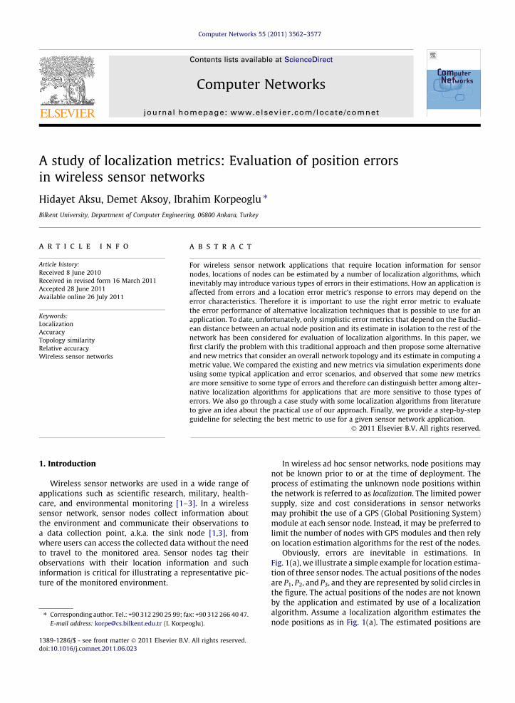
Obviously, errors are inevitable in estimations. InFig. 1(a), we illustrate a simple example for location estima-tion of three sensor nodes. The actual positions of the nodesare P1, P2, and P3, and they are represented by solid circles inthe figure. The actual positions of the nodes are not knownby the application and estimated by use of a localizationalgorithm. Assume a localization algorithm estimates thenode positions as in Fig. 1(a). The estimated positions are

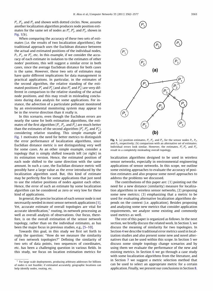
Fig. 1. (a) position estimates, P01; P02, and P03, for the sensor nodes P1, P2,

and P3, respectively; (b) comparison with an alternative set of estimates.Individual errors look similar. However, the estimates, P001; P

002, and P003,

result in a completely misleading overall topology.

H. Aksu et al. / Computer Networks 55 (2011) 3562–3577 3563

P01; P02, and P03 and shown with dotted circles. Now, assume

another localization algorithm produces node position esti-mates for the same set of nodes as P001; P

002, and P003, shown in

Fig. 1(b).When comparing the accuracy of these two sets of esti-

mates (i.e. the results of two localization algorithms), thetraditional approach uses the Euclidean distance betweenthe actual and estimated positions of the individual nodes,P1; P

01, or P001, etc. In this example, if we consider the accu-

racy of each estimate in isolation to the estimates of othernodes’ positions, this will suggest a similar error in bothcases, since the average Euclidean distance for both casesis the same. However, these two sets of estimates mayhave quite different implications for data management inpractical applications. In particular, in the estimates ofthe second algorithm, the relative standing of the esti-mated positions P001 and P002 (and also P001 and P003) are very dif-ferent in comparison to the relative standing of the actualnode positions, and this may result in misleading conclu-sions during data analysis for some applications. For in-stance, the advection of a particulate pollutant monitoredby an environmental monitoring system may appear tobe in the reverse direction than it really is.

In this scenario, even though the Euclidean errors arenearly the same for both estimation algorithms, the esti-mates of the first algorithm (P01; P

02, and P03) are much better

than the estimates of the second algorithm (P001; P002, and P003),

considering relative standing. This simple example ofFig. 1 motivates the need for better metrics to distinguishthe error performance of localization algorithms, sinceEuclidian distance metric is not distinguishing very wellfor some cases. As an other simple example, consider atopology that is simply shifted towards left (or right) inits estimation version. Hence, the estimated position ofeach node shifted to the same direction with the sameamount. In such a case, the Euclidian distance metric willpossibly have a large value as the error introduced by thelocalization algorithm used. But, this kind of estimatemay be perfectly fine for some applications that just needto use the relative positions of nodes against each other.Hence, the error of such an estimate by some localizationalgorithm can be considered as zero or very low for thesekind of applications.

In general, the precise location of each sensor node is notnecessarily needed in most sensor network applications [1].Yet, accurate estimate of overall topologies are vital foraccurate identification,1 routing, in-network processing aswell as overall analysis of observations. Our focus, there-fore, is on the overall estimation of the sensor networktopology, rather than on the individual estimates, as hasbeen the major focus in previous studies, e.g., [5–10].

Towards this goal, in this study we first set forth toreply the question: ‘‘How do we measure the similarityof two network topologies?’’ Defining the similarity oftwo sets of data points, two sequences of coordinates,etc. has been a challenging question in various fields. Inthis study, we focus on location estimation metrics for

1 For large scale deployments, producing arbitrary addresses for billionsof nodes is not feasible; if estimated accurately, geographic locations canhelp identify nodes, routing, etc.

localization algorithms designed to be used in wirelesssensor networks, especially in environmental engineeringapplications of sensor networks. In this scope, we outlinesome existing approaches to evaluate the accuracy of posi-tion estimates and also propose some novel approaches toaddress the problems we discussed.

The contributions of this paper are: (1) pointing out theneed for a new distance (similarity) measure for localiza-tion algorithms in wireless sensor networks, (2) proposingsome new metrics; (3) emphasizing that a metric to beused for evaluating alternative localization algorithms de-pends on the context (i.e. application). Besides proposingand analyzing some new metrics that consider applicationrequirements, we analyze some existing and commonlyused metrics as well.

The rest of this paper is organized as follows. In the nextsection, we briefly discuss the related work. In Section 3, wediscuss the meaning of similarity for two topologies. InSection 4 we describe traditional error metrics used in local-ization studies and also present some new and novel alter-natives that can be used within this scope. In Section 5 wediscuss some simple topology change scenarios and byusing them we evaluate the performance of the new andexisting metrics. In Section 6 we go through a case studywith some localization algorithms from the literature, andin Section 7 we suggest a metric selection method thatcan be used to select an appropriate metric for a certainapplication. Finally, we present our conclusions in Section 8.

3564 H. Aksu et al. / Computer Networks 55 (2011) 3562–3577

2. Related work

Localization is an important issue for some wirelesssensor network applications [2–4,11–14], but not all ofsuch applications require absolute positions of sensornodes. There are a lot sensor network applications or ser-vices that may do quite well with the knowledge of relativepositioning of the nodes. For example, a geographic routingor data dissemination service may work equally well if therelative positioning of the nodes against each other areknown; in other words, if the topology of the network isknown without the exact positions of the nodes. For suchapplications and services, even though some location er-rors are introduced by the estimation algorithms, thismay not be harmful for the applications provided thatthe relative positioning information is correct.

Therefore, there are various localization algorithms pro-posed for sensor networks that do not require use of GPS inevery node and that have different error performance.Those localization algorithms can be classified in variousways: range-based algorithms, range-free algorithms, re-gion-based algorithms, connectivity-based algorithms,hop-counting techniques, and so on [15–21]. There are alsosome localization techniques developed for sensor net-works where nodes can be mobile [22].

It is reported in the literature that the errors introducedby those different classes of algorithms may have differentcharacteristics. Hence, there are various types of errorsthat can be introduced by location estimation algorithms[8]. In this paper, we consider three types of errors: shit,rotational, and random (distorted) errors. There are alsostudies that investigate the impact of various types of er-rors on wireless sensor network applications [23].

Nearly all studies consider the average Euclidian dis-tance between actual and estimated node positions asthe error metric in judging the accuracy of localizationalgorithms. There are also metrics that are direct functionsof Euclidian distance, for example metrics that use the nor-malized value of the distance (normalized according to thecommunication range) [15,16,24]. There are, however, notmuch studies that consider other metrics that we argue asnecessary in this paper.

To the best of our knowledge, this paper is the first at-tempt to consider various other metrics as well while judg-ing the accuracy of localization algorithms. Some of theseother metrics are already well-known in other domains[25,26], but not much in the localization domain. Besidesthese well-known metrics, this paper also proposes somenew novel metrics that can be better to use for some appli-cations (depending on how applications tolerate varioustypes of errors) and therefore can be considered as alterna-tive metrics in localization domain. Hence, we consider ourstudy here is as an original contribution to the literature ofperformance of localization algorithms.

3. Similarity of topologies

In this study we are interested in evaluating metrics thatcompare and evaluate the difference between two sensornetwork topologies, one consisting of the actual positions

of the sensor nodes in the network, the other consisting ofthe estimated positions of the same sensor nodes by somealgorithm. To be able to do that we should first define whata topology is, so that we can define the distance or similaritybetween two topologies. It is possible to come up with var-ious definitions of a topology. One way is to consider a topol-ogy as an undirected graph G (V,E), where V is the set of nodepositions and E is set of edges so that there is an edge be-tween two nodes that are in the transmission range of eachother (assuming symmetric range). According to this defini-tion, topology depends on node positions and on the giventransmission range. Performance of localization algorithms,however, does not have to depend on a given transmissionrange. More important issue is absolute or relative nodepositions and how we estimate them. Therefore we use an-other definition of a topology in our study. We define sensornetwork topology to be a set of x-y coordinates (i.e., points ornode positions) in a two dimensional space. It is possible toextend this definition to three dimensional space consider-ing the altitude of deployed sensor nodes, but for simplicity,our discussion is confined to two-dimensional space.

More formally, when we refer to a topology T of Nnodes, we refer to a sequence of node positions P1,P2, . . . ,PN

where Pi = (xi,yi) is the coordinate of a sensor node i. Wethen refer to the estimated topology as T0 consisting of a se-quence of coordinates P01; P

02; . . . ; P0N where P0i ¼ x0i; y

0i

� �is the

estimated position of the sensor node i. We use the nota-tion dx(P,P0) to denote the distance between node positionsP and P0 (nodal/point distance or positional distance), andlx(T,T0) to denote the distance (dissimilarity) between net-work topologies T and T0 (topological distance) based onsome distance metric x.

Additionally, V!

ij ¼ PiPj

!denotes the vector from node

position Pi to node position Pj; and V!0ij ¼ P0iP

0j

!denotes the

vector from estimated node position P0i to estimated nodeposition P0j. Vector V

!ij indicates the actual relative position-

ing (arp) of two nodes i and j; and vector V!0ij indicates the

estimated relative positioning (erp) of two nodes i and j.

4. Existing and new metrics

In this section we describe different approaches andmetrics that can be used to evaluate localization algo-rithms, and in the next section, Section 5, we evaluate allthese metrics when applied to some common scenariosof topology estimations and changes.

We start this section by describing two common met-rics, Euclidian distance metric and Manhanttan distancemetric [27], currently used by localization algorithmsfollowed by the description of two other metrics, Cosinedistance metric and Tanimoto coefficient distance metric[25–27], that, to the best of our knowledge, are not appliedfor localization algorithm evaluation, but can be consid-ered as possible candidates. Then we propose and describefour novel metrics that we think can be alternative metricsfor evaluating localization algorithms designed for wirelesssensor networks and environmental engineering applica-tions: Relative Euclidian distance (RED) metric, Cumulativevectorial distance (CVD) metric, Extremes distance metric,Spring distance metric. We provide four versions of the

H. Aksu et al. / Computer Networks 55 (2011) 3562–3577 3565

Spring distance metric: Spring A, Spring B, Spring C, andSpring D distance metrics.

Besides the metrics that we consider in this paper,graph-theoretic distance metrics can be considered as well.Graphs are modeled as set of vertices (V) and edges (E) andthis model is appropriate to describe the connectivity of asensor network. However, a graph-theoretic model doesnot contain node positions which are particularly used inlocation estimation problems. Thus, graph- theoretic mod-els do not sense shift, rotation and connectivity preservingdistortion on sensor network topology. Therefore, graph-theoretic distance metrics are not considered in this paperand left as a future work.

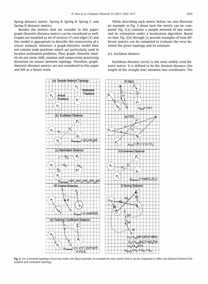
Fig. 2. For a network topology of just two nodes, the figure provides an example foriginal and estimated topology.

While describing each metric below, we also illustratean example in Fig. 2 about how the metric can be com-puted. Fig. 2(a) contains a sample network of two nodesand its estimation under a localization algorithm. Basedon that, Fig. 2(b) through (i) provide examples of how dif-ferent metrics can be computed to evaluate the error be-tween the given topology and its estimate.

4.1. Euclidean distance

Euclidean distance (error) is the most widely used dis-tance metric. It is defined to be the shortest distance (thelength of the straight line) between two coordinates. The

or each metric how it can be computed to reflect the distance between the

3566 H. Aksu et al. / Computer Networks 55 (2011) 3562–3577

Euclidean distance between two topologies can be com-puted as follows (see also Fig. 2(b)):

dEuclidian Pi; P0i

� �¼

ffiffiffiffiffiffiffiffiffiffiffiffiffiffiffiffiffiffiffiffiffiffiffiffiffiffiffiffiffiffiffiffiffiffiffiffiffiffiffiffiffiffiffiffiffixi � x0i� �2 þ yi � y0i

� �2q

; ð1Þ

lEuclidianðT; T0Þ ¼ 1

N

XN

i¼1

dEuclidian Pi; P0i

� �; ð2Þ

where xi and yi are the actual coordinates of a node i and x0iand y0i are the estimated coordinates of the node. In thisequation and in the subsequent equations for other met-rics, N is the number of nodes in the network. Above, thetopological distance lEuclidian(T,T0) indicates the error intro-duced by a localization algorithm considering all nodepositions and their estimates.

In this metric, each node position and its estimate areconsidered in isolation to other node positions and theirestimates. As we discussed in the introduction, however,since this metric does not take the direction or the relativeposition of a node with respect to other nodes in the net-work into consideration, it may not be a good metric inapplications for which estimating relative positions ismore important than estimating absolute positions. Manyscientific applications, for example, care more about rela-tive positions of reporting nodes than a few perfect posi-tion estimates - without knowing which ones.

4.2. Manhattan (Hamming) distance

Manhattan (Hamming) distance is another simple andpopular metric that is computed considering a two dimen-sional coordinate system. It is the distance between twocoordinates measured along the axes at right angles. Inother words, assuming that you can move only along thex and y-axis in the plane (not in any other arbitrary direc-tion as in the case of Euclidean distance), it measures thedistance to get from one point to the other. Similar toEuclidean distance, however, it falls short of representingrelative positioning of nodes. Below is the formula to com-pute the Manhattan distance between a topology T and itsestimate T0 (see also Fig. 2(c)).

dManhattan Pi; P0i

� �¼ x0i � xi

�� ��þ y0i � yi

�� ��� �; ð3Þ

lManhattanðT; T0Þ ¼ 1

N

XN

i¼1

dManhattan Pi; P0i

� �: ð4Þ

4.3. Cosine distance

Cosine similarity is a well-known technique that con-siders not only a single value and its estimate, but multiplevalues at the same time [25]. It is a common metric used ininformation retrieval domain. In localization domain, weconsider vectors V

!ij and V

!0ij connecting any two nodes’

actual and estimated positions. The Cosine similarity isdefined to be the cosine value of the angle (h) betweenthese two vectors (see Fig. 2(d)). In this respect it is theopposite of the Euclidian distance metric.

Note that Cosine similarity is a good metric for applica-tions that only care about the relative direction of nodesregardless of the actual distance between the pairs of esti-

mates. The absolute distance between nodes, however, isnot captured by this metric.

Cosine similarity, like other similarities, has a range of�1 to +1. We define the Cosine distance between atwo-node topology and its estimate as (1 � cosh)/2. Fora topology with more than two nodes, all pairs of nodesare considered, as shown below, to compute the topologicaldistance (Eq. (7)).

cos h ¼ Vij

!�Vij

!0

jVij

!j Vij

!0

��������; ð5Þ

dCosineðPi; PjÞ ¼1� cos h

2; ð6Þ

lCosineðT; T0Þ ¼ 2

NðN � 1ÞXN

i¼1

XN

j¼iþ1

dCosineðPi; PjÞ: ð7Þ

4.4. Tanimoto coefficient distance

Tanimoto coefficient is a more complex metric that con-siders vectors rather than points [26]. It is a highly popularmetric in text matching problems of information retrievalwhere it is defined as the size of the intersection dividedby the size of the union of the sample sets. It can beadapted to our domain as follows. We consider the pair-wise relative positions of nodes in both sets (T and T0) asvectors (see Fig. 2(e)). We then compute Tanimoto coeffi-cient (TC) of these vectors (Eq. (8)). Using the Tanimotocoeffcient, we compute the Tanimato distance (Eq. (9))for a node pair. Then the Tanimoto distance between atopology T and its estimate T0 is computed as in Eq. (10).

TCðPi; PjÞ ¼Vij

!�Vij

!0

Vij

!��������2

þ Vij

!0

��������2

� Vij

!�Vij

!0

; ð8Þ

dTanimotoðPi; PjÞ ¼1� TCðPi; PjÞ

2; ð9Þ

lTanimotoðT; T0Þ ¼ 2

NðN � 1ÞXN

i¼1

XN

j¼iþ1

dTanimotoðPi; PjÞ: ð10Þ

4.5. Relative Euclidean Distance (RED)

Relative Euclidean Distance (RED) is a novel metric thatwe propose based on our observations on how Euclideandistance fails to capture the relative position of a pair ofnodes. Euclidean distance considers a coordinate in refer-ence to the origin which is a fixed point. With RED metric,instead, we try to capture the relative positional differencebetween two sets of positions: the actual positions set andthe estimated positions set.

To compute RED metric, we consider nodes in pairs. Wefirst compute the RED of one pair. i.e. of two nodes. It isdone as follows. Considering any pair of nodes i and j inthe network and their actual (Pi,Pj) and estimated P0i; P

0j

� �positions, we first obtain the vectors V

!¼ P1P2

!and

V!0 ¼ P01P02

!. We then compute the RED metric value as the

magnitude of the vector connecting the end-points of thesetwo vectors (see Fig. 2(f) and Eq. (11)).

H. Aksu et al. / Computer Networks 55 (2011) 3562–3577 3567

The value of the metric depends on both the relativedirections of the vectors and the difference in the magni-tudes of the vectors. For example, if the estimated posi-tions are aligned along the same direction with theactual positions, we expect the angle between the two vec-tors to be relatively small, indicating that the directionalerror is low. Similarly, if the vectors have nearly the samemagnitude, then their magnitude difference will be low,indicating again a low error value.

The above process is repeated for all pairs of nodes tocompute the distance between a topology T and its esti-mate. The topological RED distance is the average of theRED distances of all pairs of nodes in the topology (Eq. (12)).

dREDðPi; PjÞ ¼ ½ðjV!j2 þ jV

!0j2 � 2 V

!�V!0Þ�1=2

; ð11Þ

lREDðT; T0Þ ¼ 2

NðN � 1ÞXN

i¼1

XN

j¼iþ1

dREDðPi; PjÞ: ð12Þ

4.6. Cumulative Vectorial Distance (CVD)

This metric we propose is motivated by Cosine similaritymetric. We aim at including distance as well as the angleinto account. First, for each node we record the differencebetween its actual and estimated x-coordinate. We repeatthe same process for the y-coordinate. We then sum upall these differences for both x and the y-coordinates andconstruct two perpendicular vectors (starting at the origin)whose magnitudes are equal to these sums respectively.The distance between the end coordinates of these vectorsis defined as the CVD metric (Fig. 2(g)). The formula belowcomputes the CVD distance between topologies T and T0:

lCVDðT; T0Þ ¼ 1

N

XN

i¼1

x0i � xi� �" #2

þXN

i¼1

y0i � yi

� �" #20@

1A

1=2

:

ð13Þ

4.7. Extremes distance

The maximum error of location estimation may have asignificant effect on some applications and the quality ofservice they get from the network and location based ser-vices running on the network. For such applications, met-rics assuring certain error bound (i.e. level of quality inlocation estimation) are necessary. Thus, we introduce Ex-tremes Distance metric which measures the distance be-tween a topology T and its estimate T0 as the maximumEuclidian distance among individual node positions andtheir estimates (see also Fig. 2(h)).

lExtremesðT; T0Þ ¼max

i21...NdEuclidian Pi; P

0i

� �� : ð14Þ

4.8. Spring distance

For this final metric we use an analogy based on a phys-ical model. We model the network topology as an elasticobject, and we consider the distance between the actualand estimated topologies as the difference in the potentialenergy of the original elastic object (corresponding to the

actual topology) and its deformed version (correspondingto the estimated topology).

Hence, we model a sensor network as an elastic objectconsisting of a set of nodes connected with springs. Eachsensor node in the model is connected to all other nodesand the ground with springs.

For a network of N nodes, there are N � 1 springs pernode connecting the node to other nodes. These springsare called Type-1 springs. Each such spring connects a pairof nodes and is responsive (stores potential energy) to achange in the Euclidean distance between those nodes.Moreover, there is one spring per node connecting the nodeto the ground. This spring is called Type-2 spring and isresponsive to the node’s individual relocation. In additionto Type-1 and Type-2 springs, which are of tension/exten-sion springs, we have an additional spring per pair of nodes,Type-3 springs, which are torsion springs. A torsion spring isa type of string that can not be extended or compressed, butcan be rotated/distorted when a force is applied. A Type-3string is responsive to a change in the direction of theType-1 spring connecting these two nodes. Since we haveone Type-3 string per pair of nodes, there are N � 1 Types-3 strings associated with a node (one string per other nodethe node is connected to with a Type-1 string). The potentialenergy stored on a Type-3 string is related with the angle ofdistortion (h) of the string (vector) connecting the corre-sponding two nodes.

We assume that all strings in the model of the actualnetwork have their relaxed length (equilibrium condition,storing zero potential energy) and then we deform thismodel into the model corresponding to the estimated net-work. We then compute the potential energy that is storedin the deformed network model, and this gives us theSpring distance. We know that the more an elastic objectis deformed, the more potential energy is stored in it.Therefore, we can consider the stored potential energy asthe measure of topological distance.

The potential energy of a tension/extension spring oflength l and elastic modulus or constant kunder compres-sion or extension of x is Ue ¼ kx2

2l . Similarly, the potential en-ergy of a torsion spring of elastic modulus or constant k withthe angle of twist (h) from its relaxed position is Ue ¼ 1

2 kh2.Spring distance between topology T and its estimate T0

is the overall potential energy stored in Type-1, Type-2and Type-3 springs (see Fig. 2(i) and Eq. (15)):

lspringðT; T0Þ ¼ UT1ðT; T 0Þ þ UT2ðT; T 0Þ þ UT3ðT; T 0Þ; ð15Þ

where

UT1ðT; T 0Þ ¼2

NðN � 1ÞXN

i¼1

XN

j¼iþ1

krel Vij

!��������� V 0ij

!��������

��������2

2jVijj; ð16Þ

UT2ðT; T 0Þ ¼1N

XN

i¼1

kshiftdEuclidian Pi; P0i

� �2

2; ð17Þ

UT3ðT; T 0Þ ¼2

NðN � 1ÞXN

i¼1

XN

j¼iþ1

12

kroth2ij; ð18Þ

hij ¼ arccosVij

!�V 0ij!

jVij

!jjV 0ij!j

0B@

1CA: ð19Þ

3568 H. Aksu et al. / Computer Networks 55 (2011) 3562–3577

UT1 computes the potential energy stored in Type-1springs under tension resulted by changes in relative loca-tion of each pair of nodes (Eq. (16)). The type-1 spring con-stant krelative is called displacement_sensitivity parameterand assumed to be 1 in the model. UT2 computes the poten-tial energy stored in Type-2 springs under tension resultedby changes in the absolute location of each individual node(Eq. (17)). The relaxed length of a Type-2 string is assumedto be 1 and the type-2 string constant, kshift, is calledshift_sensitivity parameter in the model. UT3 computes thepotential energy stored in Type-3 springs under tension re-sulted by changes in relative direction of each pair of nodes(Eq. (18)). The type-2 spring constant krotate is the rota-tional_sensitivity parameter of the model.

Computational complexity of UT2 is O(N) while it isO(N2) for UT1 and UT3. Hence computational complexityfor Spring distance is O(N2) with N nodes in the network.

Force constants of springs affect the behavior of springdistance metric. By increasing/decreasing the shift_sensi-tivity and rotation_sensitivity parameters, metric’s re-sponse to changes can be adjusted. In the simulations,we use four versions of spring distance: Spring A distanceis the one with shift_sensitivity = rotational_sensitiv-ity = 0.5; Spring B distance is the one with shift_sensitiv-ity = 1 and rotational_sensitivity = 0; Spring C distance isthe one with shift_sensitivity = 0 and rotational_sensitiv-ity = 1; Spring D distance is the one with shift_sensitiv-ity = 0 and rotational_sensitivity = 0.

5. Evaluation of metrics under sample scenarios

In this section we present some basic topology change(error) scenarios and use them to compare and evaluatethe metrics we presented in the previous section. For eachtopology change scenario studied, we discuss the impact ofthose types of errors on applications.

While some distance metrics we study give boundedvalues, e.g., Cosine distance metric, some others give un-bounded values, e.g., Euclidean distance metric. Therefore,comparing the values of the metrics directly, without anynormalization, can be misleading. Because of this we nor-malize each metric’s result with its maximum value re-ported in simulations. In this way, we can monitor thebehavior of metrics in response to the changes in the net-work topology.

We used Matlab for simulating error scenarios and eval-uating the metrics. We have written custom Matlab code tosimulate various network topologies, topology changes,and to compute the distances between the actual and chan-ged (estimated) topologies according to various metrics westudy in this paper. For our simulation experiments, wegenerate sample network topologies synthetically that aredeployed over a square area of 20 by 20 unit length. Wekeep the area size constant. We consider 10 different net-work sizes, changing from 40 nodes up to 400 nodes, witha step size of 40. For each simulation experiment, the nodesare deployed on the area with a uniform distribution. Foreach network size, the simulation experiments re repeated20 times and average results are reported. There are threebasic error scenarios that we consider: shifted topology, ro-

tated topology, distorted (random) topology. For shiftedand rotated topology simulations, actual network topologyis shifted or rotated depending on the scenario parameters,i.e., rotation angle, and then the resulting topology is usedas the estimated topology. In case of distorted topologies,three different distortion approaches are used. First, nodesare distorted by uniform distribution with various ranges.Second, nodes are distorted according to Gaussian distribu-tion with fixed mean and various sigma values. Finally,nodes are distorted by Gaussian distribution with fixed sig-ma and various mean values.

5.1. Rotated topologies

Rotated topologies are common error scenarios forenvironmental monitoring applications. We focus ontopologies that are rotated with respect to a coordinatesystem. To simulate such a topology change scenario, weplace all nodes on a plane and then rotate the plane so thatthe distance between any two nodes stay exactly the samewhile the overall alignment differs.

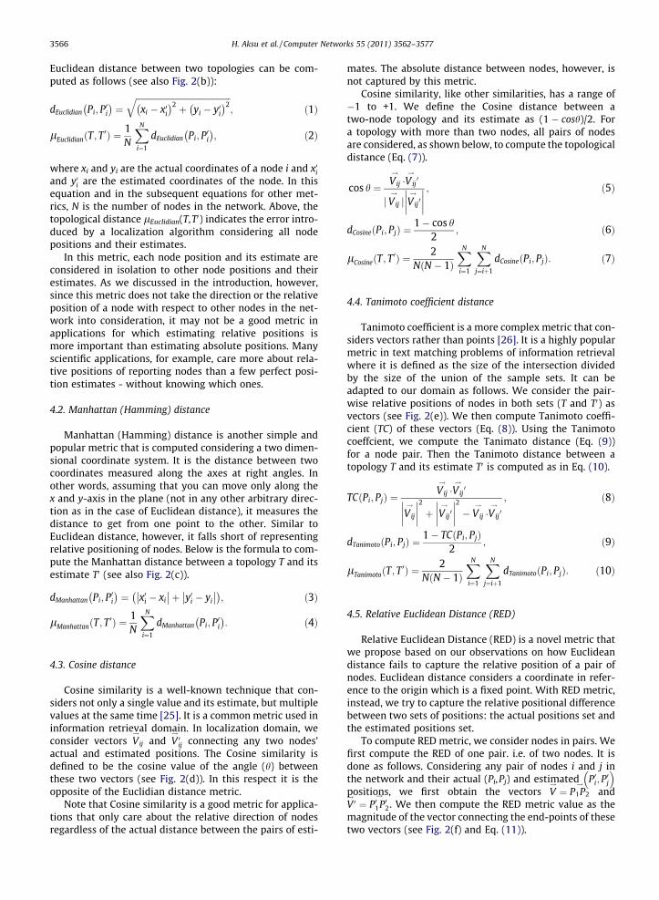
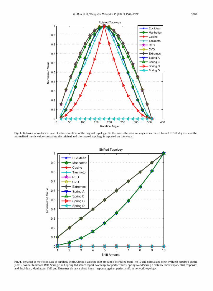
We run simulations for various rotations by increasingthe angle of rotation. In Fig. 3, the distance between the ori-ginal and estimated topology is plotted for various metricsas rotation angle increases. As can be seen from the figure,all metrics, except Spring D metric, report an increasing er-ror as the angle increases up to 180 degrees. The behavior isfully symmetric for all metrics studied, reaching a peak er-ror at 180 degrees and returning back to zero error at 360degrees, which reflects the original topology.

In traditional pattern matching problems, we would ex-pect similarity degrees to be high in rotated topologiessince the shape on the plane does not change when we ro-tate the plane. Yet, in environmental engineering applica-tions the reference to the coordinate system does play asignificant role in the interpretation of the observationsfrom the network.

As seen in Fig. 3, Spring C metric increases exponen-tially while Tanimoto, Cosine, Spring A, Spring B metricsincrease linearly and Euclidean, Manhattan, Extremes andCVD metrics increase logarithmically while the angle ofrotation is increased from 0 to 180 degrees. In this regard,among all metrics, Spring C seems to be the most sensitivemetric for rotated topologies. On the other hand, Spring Ddistance metric is not sensitive to rotation operation at all.

5.2. Shifted topologies

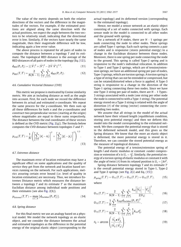
The second error scenario we consider is a topologywith a perfect shift. That is all nodes in the network aresubject to the exact distortion in a particular direction.For instance, all nodes deployed on a lake surface may havemoved northeast by forces of wind after location estima-tion. We simulate this scenario by taking the estimatedlocation for a node as (x + n,y + n), where (x,y) is the origi-nal coordinate of the node and n is a number representingthe shift amount, between 1 and 10, in both x and y dimen-sions. Even though this is a rather simplified assumption,i.e., in practice some nodes can move more than the others,the scenario will help us to observe the behavior of metricsfor the general case of shifted topologies.

0 50 100 150 200 250 300 350 4000

0.1

0.2

0.3

0.4

0.5

0.6

0.7

0.8

0.9

1

Rotation Angle

Nor

mal

ized

Val

ue

Rotated Topology

EuclideanManhattanCosineTanimotoREDCVDExtremesSpring ASpring BSpring CSpring D

Fig. 3. Behavior of metrics in case of rotated replicas of the original topology: On the x-axis the rotation angle is increased from 0 to 360 degrees and thenormalized metric value comparing the original and the rotated topology is reported on the y-axis.

1 2 3 4 5 6 7 8 9 100

0.1

0.2

0.3

0.4

0.5

0.6

0.7

0.8

0.9

1

Shift Amount

Nor

mal

ized

Val

ue

Shifted Topology

EuclideanManhattanCosineTanimotoREDCVDExtremesSpring ASpring BSpring CSpring D

Fig. 4. Behavior of metrics in case of topology shifts. On the x-axis the shift amount is increased from 1 to 10 and normalized metric value is reported on they-axis. Cosine, Tanimoto, RED, Spring C and Spring D distance report no change for perfect shifts. Spring A and Spring B distance show exponential response;and Euclidean, Manhattan, CVD and Extremes distance show linear response against perfect shift in network topology.

H. Aksu et al. / Computer Networks 55 (2011) 3562–3577 3569

0 2 4 6 8 10 12 14 16 18 200

0.1

0.2

0.3

0.4

0.5

0.6

0.7

0.8

0.9

1

Range

Nor

mal

ized

Val

ue

Distorted Topology 1

EuclideanManhattanCosineTanimotoREDCVDExtremesSpring ASpring BSpring CSpring D

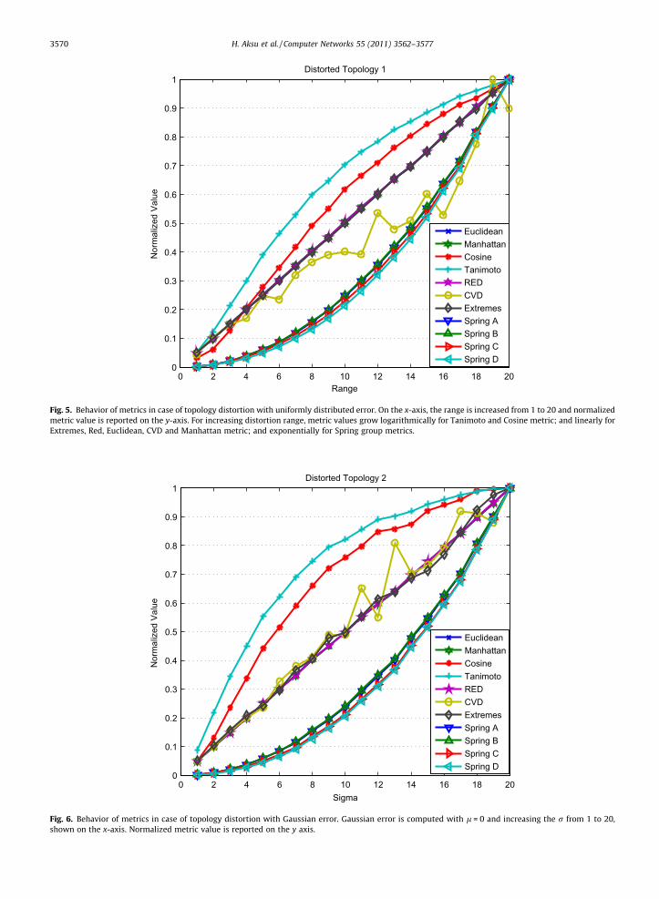
Fig. 5. Behavior of metrics in case of topology distortion with uniformly distributed error. On the x-axis, the range is increased from 1 to 20 and normalizedmetric value is reported on the y-axis. For increasing distortion range, metric values grow logarithmically for Tanimoto and Cosine metric; and linearly forExtremes, Red, Euclidean, CVD and Manhattan metric; and exponentially for Spring group metrics.

0 2 4 6 8 10 12 14 16 18 200

0.1

0.2

0.3

0.4

0.5

0.6

0.7

0.8

0.9

1

Sigma

Nor

mal

ized

Val

ue

Distorted Topology 2

EuclideanManhattanCosineTanimotoREDCVDExtremesSpring ASpring BSpring CSpring D

Fig. 6. Behavior of metrics in case of topology distortion with Gaussian error. Gaussian error is computed with l = 0 and increasing the r from 1 to 20,shown on the x-axis. Normalized metric value is reported on the y axis.

3570 H. Aksu et al. / Computer Networks 55 (2011) 3562–3577

H. Aksu et al. / Computer Networks 55 (2011) 3562–3577 3571

Fig. 4 shows the values of various distance metrics asthe amount of the shift (n) is increased on the x-axis. Asseen, even though the complete topology (graph represen-tation of the network) is preserved perfectly, Euclidean,Manhattan, CVD, Extremes, Spring A and Spring B distancemetrics respond the change. Among these matrices, SpringA and Spring B distance report a distance that is exponen-tially related to the shift amount, while other metrics re-port an error that is linearly related to the shift amount.On the other hand, Cosine, Tanimoto, RED, Spring C andSpring D distance metrics report no change for perfectshifts. In shifted topologies, even though the absolute loca-tion of nodes is changing, it may not be a major concern formany expert applications. In most cases, shifts that main-tain the relative positioning of nodes are acceptable forenvironmental monitoring applications. For instance, apollutant flow in northeast direction will still appear inthe same direction if all nodes maintain their relativepositioning.

5.3. Distorted topologies

Distorted topologies represent arbitrary errors made inposition estimates. In this category we study a scenariowhere node positions are shifted along statistically. We ap-ply an independent distortion to each node such that theresulting topology will have some relative accuracy errors.First, we introduce uniformly distributed distortion oneach node, where size of the range of distortion changes

0 2 4 6 8 10

0.1

0.2

0.3

0.4

0.5

0.6

0.7

0.8

0.9

1

Me

Nor

mal

ized

Val

ue

Distorted

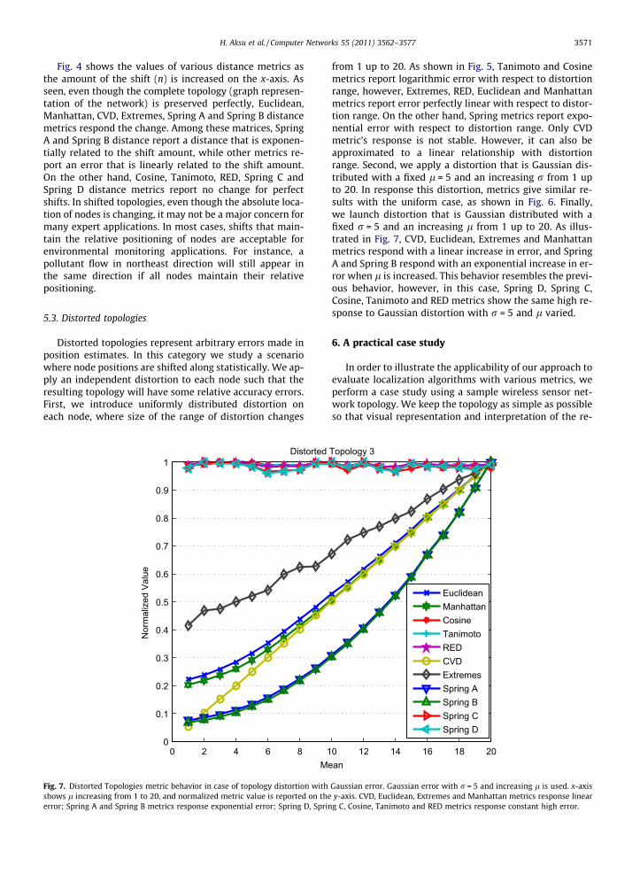
Fig. 7. Distorted Topologies metric behavior in case of topology distortion withshows l increasing from 1 to 20, and normalized metric value is reported on theerror; Spring A and Spring B metrics response exponential error; Spring D, Sprin

from 1 up to 20. As shown in Fig. 5, Tanimoto and Cosinemetrics report logarithmic error with respect to distortionrange, however, Extremes, RED, Euclidean and Manhattanmetrics report error perfectly linear with respect to distor-tion range. On the other hand, Spring metrics report expo-nential error with respect to distortion range. Only CVDmetric’s response is not stable. However, it can also beapproximated to a linear relationship with distortionrange. Second, we apply a distortion that is Gaussian dis-tributed with a fixed l = 5 and an increasing r from 1 upto 20. In response this distortion, metrics give similar re-sults with the uniform case, as shown in Fig. 6. Finally,we launch distortion that is Gaussian distributed with afixed r = 5 and an increasing l from 1 up to 20. As illus-trated in Fig. 7, CVD, Euclidean, Extremes and Manhattanmetrics respond with a linear increase in error, and SpringA and Spring B respond with an exponential increase in er-ror when l is increased. This behavior resembles the previ-ous behavior, however, in this case, Spring D, Spring C,Cosine, Tanimoto and RED metrics show the same high re-sponse to Gaussian distortion with r = 5 and l varied.

6. A practical case study

In order to illustrate the applicability of our approach toevaluate localization algorithms with various metrics, weperform a case study using a sample wireless sensor net-work topology. We keep the topology as simple as possibleso that visual representation and interpretation of the re-

0 12 14 16 18 20an

Topology 3

EuclideanManhattanCosineTanimotoREDCVDExtremesSpring ASpring BSpring CSpring D

Gaussian error. Gaussian error with r = 5 and increasing l is used. x-axisy-axis. CVD, Euclidean, Extremes and Manhattan metrics response linearg C, Cosine, Tanimoto and RED metrics response constant high error.

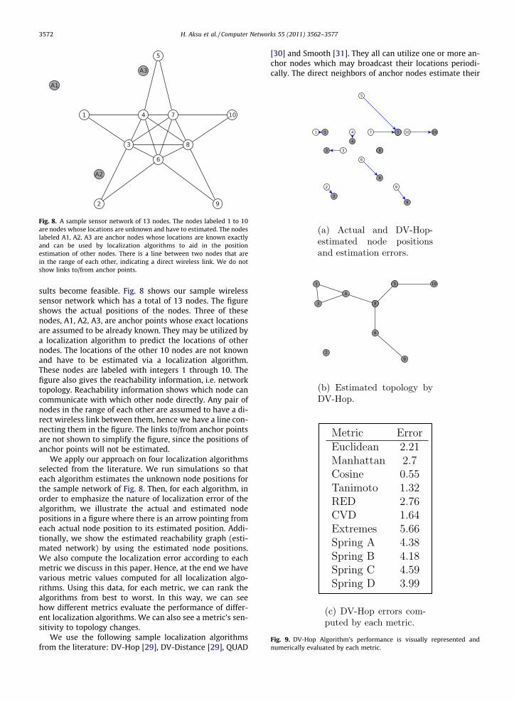
Fig. 8. A sample sensor network of 13 nodes. The nodes labeled 1 to 10are nodes whose locations are unknown and have to estimated. The nodeslabeled A1, A2, A3 are anchor nodes whose locations are known exactlyand can be used by localization algorithms to aid in the positionestimation of other nodes. There is a line between two nodes that arein the range of each other, indicating a direct wireless link. We do notshow links to/from anchor points.

Fig. 9. DV-Hop Algorithm’s performance is visually represented andnumerically evaluated by each metric.

3572 H. Aksu et al. / Computer Networks 55 (2011) 3562–3577

sults become feasible. Fig. 8 shows our sample wirelesssensor network which has a total of 13 nodes. The figureshows the actual positions of the nodes. Three of thesenodes, A1, A2, A3, are anchor points whose exact locationsare assumed to be already known. They may be utilized bya localization algorithm to predict the locations of othernodes. The locations of the other 10 nodes are not knownand have to be estimated via a localization algorithm.These nodes are labeled with integers 1 through 10. Thefigure also gives the reachability information, i.e. networktopology. Reachability information shows which node cancommunicate with which other node directly. Any pair ofnodes in the range of each other are assumed to have a di-rect wireless link between them, hence we have a line con-necting them in the figure. The links to/from anchor pointsare not shown to simplify the figure, since the positions ofanchor points will not be estimated.

We apply our approach on four localization algorithmsselected from the literature. We run simulations so thateach algorithm estimates the unknown node positions forthe sample network of Fig. 8. Then, for each algorithm, inorder to emphasize the nature of localization error of thealgorithm, we illustrate the actual and estimated nodepositions in a figure where there is an arrow pointing fromeach actual node position to its estimated position. Addi-tionally, we show the estimated reachability graph (esti-mated network) by using the estimated node positions.We also compute the localization error according to eachmetric we discuss in this paper. Hence, at the end we havevarious metric values computed for all localization algo-rithms. Using this data, for each metric, we can rank thealgorithms from best to worst. In this way, we can seehow different metrics evaluate the performance of differ-ent localization algorithms. We can also see a metric’s sen-sitivity to topology changes.

We use the following sample localization algorithmsfrom the literature: DV-Hop [29], DV-Distance [29], QUAD

[30] and Smooth [31]. They all can utilize one or more an-chor nodes which may broadcast their locations periodi-cally. The direct neighbors of anchor nodes estimate their

H. Aksu et al. / Computer Networks 55 (2011) 3562–3577 3573

positions based on received signal strength value and theypropagate their estimates to non-neighbor nodes that aremultiple-hops away from the anchor nodes. The algo-rithms differ in how they propagate the estimations andin the approach used by the rest of network to estimatethe distances and positions of the remaining nodes.

We simulated these localization algorithms over oursample topology and estimated node positions. The resultsare presented in Figs. 9–12. Each figure is about the resultsof a different localization algorithm and each figure has 3sub-parts. In part (a) we show the actual and estimatednode positions, in (b) we show the estimated topology(network), and in (c) we show localization error valuesaccording to various metrics.

Results for DV-Hop [29] algorithm are demonstrated inFig. 9. Fig. 9(a) shows that DV-Hop localization algorithm’sestimation contains errors in east–west–south directions

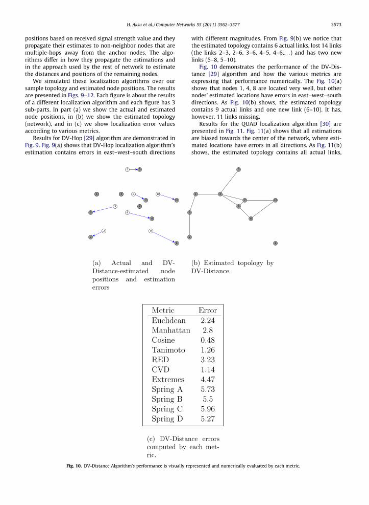
Fig. 10. DV-Distance Algorithm’s performance is visually re

with different magnitudes. From Fig. 9(b) we notice thatthe estimated topology contains 6 actual links, lost 14 links(the links 2–3, 2–6, 3–6, 4–5, 4–6,. . .) and has two newlinks (5–8, 5–10).

Fig. 10 demonstrates the performance of the DV-Dis-tance [29] algorithm and how the various metrics areexpressing that performance numerically. The Fig. 10(a)shows that nodes 1, 4, 8 are located very well, but othernodes’ estimated locations have errors in east–west–southdirections. As Fig. 10(b) shows, the estimated topologycontains 9 actual links and one new link (6–10). It has,however, 11 links missing.

Results for the QUAD localization algorithm [30] arepresented in Fig. 11. Fig. 11(a) shows that all estimationsare biased towards the center of the network, where esti-mated locations have errors in all directions. As Fig. 11(b)shows, the estimated topology contains all actual links,

presented and numerically evaluated by each metric.

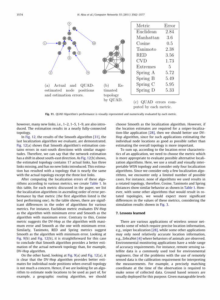
Fig. 11. QUAD Algorithm’s performance is visually represented and numerically evaluated by each metric.

3574 H. Aksu et al. / Computer Networks 55 (2011) 3562–3577

however, many new links, i.e., 1–2, 1–5, 1–9, are also intro-duced. The estimation results in a nearly fully-connectedtopology.

In Fig. 12, the results of the Smooth algorithm [31], thelast localization algorithm we evaluate, are demonstrated.Fig. 12(a) shows that Smooth algorithm’s estimation con-tains errors in east-south directions with similar magni-tudes. Therefore, we can say that the network estimationhas a shift in about south-east direction. As Fig. 12(b) shows,the estimated topology contains 17 actual links, has threelinks missing, and has no new links introduced. This estima-tion has resulted with a topology that is nearly the samewith the actual topology except the three lost links.

After computing the localization errors of these algo-rithms according to various metrics, we create Table 1. Inthis table, for each metric discussed in the paper, we listthe localization algorithms in ascending order of error per-formance by that metric (the first algorithm listed is thebest performing one). As the table shows, there are signif-icant differences in the order of algorithms for variousmetrics. For instance, Euclidean metric evaluates DV-Hopas the algorithm with minimum error and Smooth as thealgorithm with maximum error. Contrary to this, Cosinemetric suggests the DV-Hop as the algorithm with maxi-mum error and Smooth as the one with minimum error.Similarly, Tanimoto, RED and Spring metrics suggestSmooth as the algorithm with minimum error. Looking atFig. 9(b) and Fig. 12(b), it is straightforward for this caseto conclude that Smooth algorithm provides a better esti-mation of the actual network topology than, for example,DV-Hop algorithm.

On the other hand, looking at Fig. 9(a) and Fig. 12(a), itis clear that the DV-Hop algorithm provides better esti-mates for individual node positions when overall topologyis not much a concern. Hence, if we are looking for an algo-rithm to estimate node locations to be used as part of, forexample, a geographic routing algorithm, we should

choose Smooth as the localization algorithm. However, ifthe location estimates are required for a sniper-localiza-tion-like application [28], then we should better use DV-Hop algorithm, since for such applications estimating theindividual node locations as good as possible rather thanestimating the overall topology is more important.

To sum up, according to the location error characteris-tics of an application, we need to choose the metric whichis more appropriate to evaluate possible alternative locali-zation algorithms. Here, we use a small and visually inter-pretable WSN topology and consider only four localizationalgorithms. Since we consider only a few localization algo-rithms, we encounter only a limited number of possiblecases. For instance, none of algorithms we used results ina rotated topology, therefore, Cosine, Tanimoto and Springdistances show similar behavior as shown in Table 1. How-ever, with some other algorithms that would result in ro-tated topologies, we would expect more significantdifferences in the values of these metrics, considering thesimulation results shown in Fig. 3.

7. Lessons learned

There are various applications of wireless sensor net-works some of which require precise location information,e.g., sniper localization [28], while some other applicationsmay only need relatively accurate location information,e.g., ZebraNet [4] where behaviors of animals are observed.Environmental monitoring applications have a wide rangeof accuracy requirements. For instance, remote sensing sa-tellite data is a commonly used tool for environmentalengineers. One of the problems with the use of remotelysensed data is the calibration requirement for interpretingthe measurements. For example, a precisely matchingcoordinate at the time of the observation is required tomake sense of collected data. Ground based sensors areusually deployed for this purpose. Given manageable levels

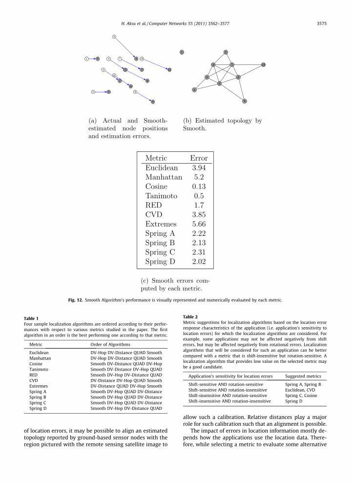
Fig. 12. Smooth Algorithm’s performance is visually represented and numerically evaluated by each metric.

Table 1Four sample localization algorithms are ordered according to their perfor-mances with respect to various metrics studied in the paper. The firstalgorithm in an order is the best performing one according to that metric.

Metric Order of Algorithms

Euclidean DV-Hop DV-Distance QUAD SmoothManhattan DV-Hop DV-Distance QUAD SmoothCosine Smooth DV-Distance QUAD DV-HopTanimoto Smooth DV-Distance DV-Hop QUADRED Smooth DV-Hop DV-Distance QUADCVD DV-Distance DV-Hop QUAD SmoothExtremes DV-Distance QUAD DV-Hop SmoothSpring A Smooth DV-Hop QUAD DV-DistanceSpring B Smooth DV-Hop QUAD DV-DistanceSpring C Smooth DV-Hop QUAD DV-DistanceSpring D Smooth DV-Hop DV-Distance QUAD

Table 2Metric suggestions for localization algorithms based on the location errorresponse characteristics of the application (i.e. application’s sensitivity tolocation errors) for which the localization algorithms are considered. Forexample, some applications may not be affected negatively from shifterrors, but may be affected negatively from rotational errors. Localizationalgorithms that will be considered for such an application can be bettercompared with a metric that is shift-insensitive but rotation-sensitive. Alocalization algorithm that provides low value on the selected metric maybe a good candidate.

Application’s sensitivity for location errors Suggested metrics

Shift-sensitive AND rotation-sensitive Spring A, Spring BShift-sensitive AND rotation-insensitive Euclidean, CVDShift-insensitive AND rotation-sensitive Spring C, CosineShift-insensitive AND rotation-insensitive Spring D

H. Aksu et al. / Computer Networks 55 (2011) 3562–3577 3575

of location errors, it may be possible to align an estimatedtopology reported by ground-based sensor nodes with theregion pictured with the remote sensing satellite image to

allow such a calibration. Relative distances play a majorrole for such calibration such that an alignment is possible.

The impact of errors in location information mostly de-pends how the applications use the location data. There-fore, while selecting a metric to evaluate some alternative

3576 H. Aksu et al. / Computer Networks 55 (2011) 3562–3577

localization algorithms and their errors, characteristics ofthe location information required by an application shouldbe considered as well. Note that, the maximization or min-imization of a metric value is not significant by itself. Thebehavior of the metric response against the types ofchanges in the estimated network topology with respectto the original topology is also important. Therefore, weaggregate the simulation results and analyze them to clas-sify the metric’s behavior in a sensitivity table. For thetopology change scenarios we simulated, we create groupsof metrics responses we have learned from simulations,such as shift sensitive ones. We favor exponential over lin-ear and linear over logarithmic response behavior by givingassigning weights from high to low. Then we obtain theTable 2 by performing appropriate set operations. Forinstance, we decide about shift and rotate sensitive metricsby intersection of shift sensitive group and rotationsensitive group with highest weight. As a result of this,for example, we decide to use Spring A and Spring B dis-tance which have exponential sensitivity for shift typechanges and linear sensitivity for rotation type changes.

For a planned wireless sensor network application, wesuggest first identifying and listing the characteristics ofthe required location data based on its sensitivity to shiftand rotation errors. For this purpose, we categorize errorsaccording to a reference coordinate in the deploymentplane. Then, appropriate metric can be chosen by lookingup the Table 2, in which we suggest metrics according toapplication requirements on location data errors of algo-rithms. Subsequently, candidate algorithms may be simu-lated, and their performance is evaluated by the chosendistance metric. Finally, the localization algorithm whichis the most appropriate for the planned application is readyto be picked up.

8. Conclusions

A number of algorithms have been proposed for thelocalization problem in wireless sensor networks. Yet, theevaluation of these algorithms traditionally depends onfairly simplistic metrics based on the original and the esti-mated coordinates of each node in isolation to the rest ofthe network. In this paper, we first discussed the implica-tions of errors considering the expectations of end users.We then discussed that there is a need for new metrics thatwill consider the relative positioning of each node with re-spect to other nodes for accurate data analysis. We thenstudied and proposed alternative distance metrics to eval-uate localization algorithms. We studied various metricsusing some basic topology change (error) scenarios to pro-vide an understanding of how the metrics respond to var-ious type of errors and what can be the implications ofthese responses to end user applications. We also dis-cussed the advantages of one metric with respect to otherones for some specific applications. We provide a casestudy, in which we evaluate some localization algorithmsfrom literature using various metrics, to show the applica-bility of our approach. At the end, we suggest a metricselection methodology that is summarized into a tableand that can consider the localization requirements ofapplications.

Acknowledgements

This work is supported in part by European Union FP7Framework Program FIRESENSE Project 244088.

References

[1] I. Akyildiz, W. Su, Y. Sankarasubramaniam, E. Cayirci, A survey onsensor networks, IEEE Communications Magazine 40 (8) (2002) 102–114.

[2] H. Alemdar, C. Ersoy, Wireless sensor networks for healthcare: asurvey, Computer Networks 54 (2010) 2688–2710.

[3] J. Yick, B. Mukherjee, D. Ghosal, Wireless sensor network survey,Computer Networks 52 (12) (2008) 2292–2330.

[4] P. Juang, H. Oki, Y. Wang, M. Martonosi, L.-S. Peh, D. Rubenstein,Energy-efficient computing for wildlife tracking: design tradeoffsand early experiences with zebranet, in: ASPLOS: Proceedings of the10th International Conference on Architectural Support forProgramming Languages and Operating Systems, New York, USA,2002, pp. 96–107.

[5] L. Lazos, R. Poovendra, SeRLoc: secure range-independentlocalization for wireless sensor networks, in: Proceedings of theACM Workshop on Wireless Security, Editors: Markus Jakobsson andAdrian Perrig, New York, USA, 2004, pp. 21–30.

[6] D.C. Moore, J.J. Leonard, D. Rus, S.J. Teller, Robust distributed networklocalization with noisy range measurements, in: Proceedings of the2nd International Conference on Embedded Networked SensorSystems, Baltimore, MD, USA, 2004, pp. 50–61.

[7] R. Nagpal, H. Shrobe, J. Bachrach, Organizing a global coordinatesystem from local information on an ad hoc sensor network, in:Proceedings of 2nd International Workshop on InformationProcessing in Sensor Networks, Lecture Notes in Computer Science,vol. 634, Springer, 2003, pp. 333–348.

[8] D. Niculescu, B. Nath, Error characteristics of ad hoc positioningsystems, in: Proceedings of the 5th ACM international symposium onMobile ad hoc Networking and Computing (MobiHoc), New York, NY,USA, 2004, pp. 20–30.

[9] C. Savarese, J. Rabaey, J. Beutel, Locationing in distributed ad-hocwireless sensor networks, in: IEEE International Conference onAcoustics, Speech, and Signal Processing (ICASSP), Salt Lake City,UT, USA, 2001, pp. 2037–2040.

[10] M. Wong, D. Aksoy, Relative accuracy based location estimation inwireless ad hoc sensor networks, in: IEEE ICC, Glasgow, 2007, pp.3244–3250.

[11] X. Wanga, O. Bischoffa, R, Laura, S. Paula, Localization in wireless ad-hoc sensor networks using multilateration with RSSI for logisticapplications, in: Proceedings of the Eurosensors XXIII Conference,Procedia Chemistry, vol. 1, 2009, pp. 461–464.

[12] S.-R. Hua, S. Peeta, C.-H. Chu, Identification of vehicle sensorlocations for link-based network traffic applications,Transportation Research Part B 43 (2009) 873–894.

[13] K.-P. Shih, S.-S. Wang, H.-C. Chen, P.-H. Yang, CollECT: collaborativeevent detection and tracking in wireless heterogeneous sensornetworks, Computer Communications 31 (2008) 3124–3136.

[14] S.-M. Lee, H. Cha, R. Ha, Energy-aware location error handling forobject tracking applications in wireless sensor networks, ComputerCommunications 30 (2007) 1443–1450.

[15] S. Zhang, J. Cao, Y. Zeng, Z. Li, L. Chen, D. Chen, On accuracy of regionbased localization algorithms for wireless sensor networks,Computer Communications 33 (12) (2010) 1391–1403.

[16] M. Boushaba, A. Hafid, A. Benslimane, High accuracy localizationmethod using AoA in sensor networks, Computer Networks 53 (18)(2009) 3076–3088.

[17] G. Mao, B. Fidan, B.D.O. Anderson, Wireless sensor network locali-zation techniques, Computer Networks 51 (10) (2007) 2529–2553.

[18] S.-S. Wang, K.-P. Shih, C.-Y. Chang, Distributed direction-basedlocalization in wireless sensor networks, ComputerCommunications 30 (6) (2007) 1424–1439.

[19] D. Niculescu, B. Nath, DV based positioning in ad hoc networks,Kluwer Journal of Telecommunication Systems 22 (1) (2003) 267–280.

[20] G.J. Jordt, R.O. Baldwin, J.F. Raquet, B.E. Mullins, Energy cost anderror performance of range-aware, anchor-free localizationalgorithms, Ad Hoc Networks 6 (4) (2008) 539–559.

[21] Y. Ding, C. Wang, L. Xiao, Using mobile beacons to locate sensors inobstructed environments, Journal of Parallel Distributed Computing70 (6) (2010) 644–656.

H. Aksu et al. / Computer Networks 55 (2011) 3562–3577 3577

[22] L. Hu, D. Evans, Localization for mobile sensor networks, in:Proceedings of the Tenth Annual International Conference onMobile Computing and Networking (MobiCom 2004), Philadelphia,USA, 2004.

[23] D. Al-Abri, J. McNair, On the interaction between localization andlocation verification for wireless sensor networks, ComputerNetworks 52 (14) (2008) 2713–2727.

[24] M. Erol-Kantarci, S. Oktug, L. Vieira, M. Gerla, Performanceevaluation of distributed localization techniques for mobileunderwater acoustic sensor networks, Ad Hoc Networks 9 (1)(2011) 61–72.

[25] G. Salton, M.J. McGill, Introduction to Modern Information Retrieval,McGraw-Hill, New York, 1983.

[26] D.R. Flower, On the properties of bit string-based measures ofchemical similarity, Journal of Chemical Information and ComputerSciences 38 (3) (1998) 379–386.

[27] R. Duda, P. Hart, D. Stork, Pattern Classification, second ed., JohnWiley and Sons, 2001.

[28] G. Simon, M. Maroti, A. Ledeczi, G. Balogh, B. Kusy, A. Nadas, G. Pap, J.Sallai, K. Frampton, Sensor network-based countersniper system, in:Proceedings of the 2nd International Conference on EmbeddedNetworked Sensor Systems (SenSys04), New York, USA, 2004, pp. 1–12.

[29] D. Niculescu, B. Nath, Ad hoc positioning system (APS), in: GlobalTelecommunications Conference, 2001, GLOBECOM ’01 IEEE, vol. 5,2001, pp. 2926–2931.

[30] M. Wong, D. Aksoy, QUAD: Quadrant-based relative locationestimates for representative topologies in wireless sensornetworks, Computer Networks 53 (12) (2009) 1967–1979.

[31] R. Nagpal, H. Shrobe, J. Bachrach, Organizing a global coordinatesystem from local information on an ad hoc sensor network, in:Proceedings of Second International Workshop on InformationProcessing and Sensor Networks, 2003.

Hidayet Aksu is a Ph.D. student in Depart-ment of Computer Engineering, Bilkent Uni-versity, Turkey. He received his M.S. and B.S.degrees again from Department of ComputerEngineering of Bilkent University. Hisresearch interests include wireless networks,wireless ad hoc and sensor networks, locali-zation, and p2p networks.

Demet Aksoy is a computer science consul-tant at Silicon Valley who specializes inproblems of wireless communications meet-ing information management. She receivedher Ph.D. (doctoral degree) in Computer Sci-ence from University of Maryland, CollegePark. She has more than 15 years of expertisein IT and has been managing diverse projectsthat mainly focus around wireless informa-tion management. Her recent project experi-ence includes information distribution inresource-contrained wireless devices, location

estimation in ad hoc networks, self-organization in sensor networks, andmutlimedia over wireless. She is certified in project management, PMP(Project Management Professional), by PMI.

Ibrahim Korpeoglu received his Ph.D. andM.S. degrees from University of Maryland atCollege Park, both in Computer Science, in2000 and 1996, respectively. He received hisB.S. degree in Computer Engineering fromBilkent University in 1994. He joined BilkentUniversity in 2002, and he is an AssociateProfessor in the Department of ComputerEngineering. Before that, he worked in severalresearch and development companies in USAincluding Ericsson, IBM T.J. Watson ResearchCenter, Bell Laboratories, and Bell Communi-

cations Research (Bellcore). He received Bilkent University DistinguishedTeaching Award in 2006 and IBM Faculty Award in 2009. He is a memberof ACM and a senior member of IEEE.