Embed Size (px)
Citation preview

A Study of Globular Cluster Systems in the Shapley Supercluster Region with the
Hubble Space Telescope
by
REGINA G. BARBER DEGRAAFF
A dissertation submitted in partial fulfillment of
the requirements for the degree of
Doctor of Philosophy
WASHINGTON STATE UNIVERSITY
Department of Physics and Astronomy
August 2011

To the Faculty of Washington State University:
The members of the Committee appointed to examine the dissertation of Regina G.
Barber DeGraaff find it satisfactory and recommend that it be accepted.
John P. Blakeslee, Ph.D., Chair
Michael Allen, Ph.D.
Philip Marston, Ph.D.
Guy Worthy, Ph.D.
ii
Abstract
A Study of Globular Clusters Systems in the Shapley Supercluster Region with the
Hubble Space Telescope
by Regina G. Barber DeGraaff, Ph.D.
Washington State University
August 2011
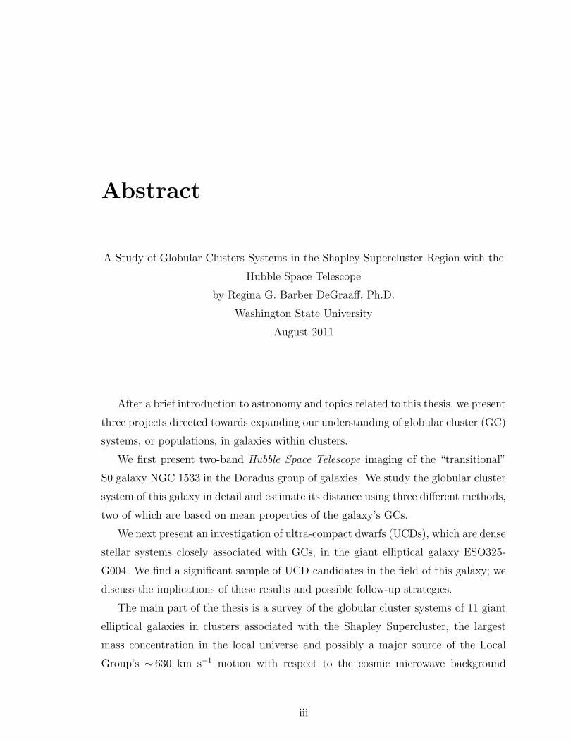
After a brief introduction to astronomy and topics related to this thesis, we present
three projects directed towards expanding our understanding of globular cluster (GC)
systems, or populations, in galaxies within clusters.
We first present two-band Hubble Space Telescope imaging of the “transitional”
S0 galaxy NGC 1533 in the Doradus group of galaxies. We study the globular cluster
system of this galaxy in detail and estimate its distance using three different methods,
two of which are based on mean properties of the galaxy’s GCs.
We next present an investigation of ultra-compact dwarfs (UCDs), which are dense
stellar systems closely associated with GCs, in the giant elliptical galaxy ESO325-
G004. We find a significant sample of UCD candidates in the field of this galaxy; we
discuss the implications of these results and possible follow-up strategies.
The main part of the thesis is a survey of the globular cluster systems of 11 giant
elliptical galaxies in clusters associated with the Shapley Supercluster, the largest
mass concentration in the local universe and possibly a major source of the Local
Group’s ∼ 630 km s−1 motion with respect to the cosmic microwave background
iii
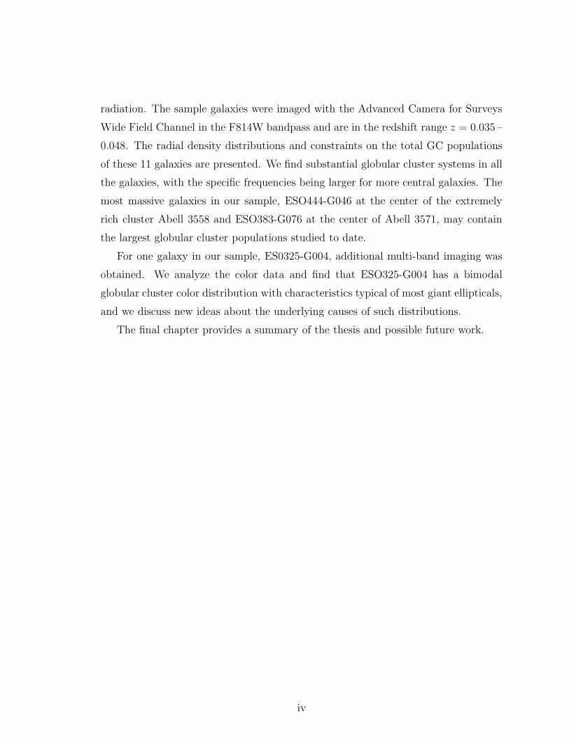
radiation. The sample galaxies were imaged with the Advanced Camera for Surveys
Wide Field Channel in the F814W bandpass and are in the redshift range z = 0.035 –
0.048. The radial density distributions and constraints on the total GC populations
of these 11 galaxies are presented. We find substantial globular cluster systems in all
the galaxies, with the specific frequencies being larger for more central galaxies. The
most massive galaxies in our sample, ESO444-G046 at the center of the extremely
rich cluster Abell 3558 and ESO383-G076 at the center of Abell 3571, may contain
the largest globular cluster populations studied to date.
For one galaxy in our sample, ES0325-G004, additional multi-band imaging was
obtained. We analyze the color data and find that ESO325-G004 has a bimodal
globular cluster color distribution with characteristics typical of most giant ellipticals,
and we discuss new ideas about the underlying causes of such distributions.
The final chapter provides a summary of the thesis and possible future work.
iv
Acknowledgements
I would like to thank my advisor, John Blakeslee for his infinite patience and help.
He may be the nicest astrophysicist alive. The members of the University of Washing-
ton Astronomy Department deserve thanks for offering me words of encouragement
and office space during part of this thesis. Instruction at McMaster University by
William Harris on DAOphot was essential for Chapter 4 and I thank him immensely.
Special thanks to family and friends for being understanding through these stress-
ful years. Thank you to my parents for taking care of me by cleaning, cooking,
babysitting, taking me on undeserved trips, and believing in me. Lastly, I would like
to thank my husband for putting up with me while I went crazy because of this thesis
and my daughter for being so cute that it made me forget about the pressure.
v
Contents
Abstract iii
Acknowledgements v
List of Figures x
List of Tables xxiii
1 Introduction 1
1.1 Globular Clusters . . . . . . . . . . . . . . . . . . . . . . . . . . . . . 2
1.1.1 History . . . . . . . . . . . . . . . . . . . . . . . . . . . . . . . 2
1.2 Distance Indicators . . . . . . . . . . . . . . . . . . . . . . . . . . . . 7
1.2.1 Geometic Parallax . . . . . . . . . . . . . . . . . . . . . . . . 7
1.2.2 Hipparcus, Magnitude Scale and Distance Modulus . . . . . . 11
1.2.3 Filters and Color . . . . . . . . . . . . . . . . . . . . . . . . . 12
1.2.4 Standard Candles . . . . . . . . . . . . . . . . . . . . . . . . . 12
1.2.5 Globular Cluster Luminosity Function . . . . . . . . . . . . . 13
1.2.6 Surface Brightness Fluctuation . . . . . . . . . . . . . . . . . 14
1.2.7 GC Size . . . . . . . . . . . . . . . . . . . . . . . . . . . . . . 14
1.2.8 Redshift and Hubble’s Law . . . . . . . . . . . . . . . . . . . . 14
1.3 Galaxy Types . . . . . . . . . . . . . . . . . . . . . . . . . . . . . . . 15
1.3.1 Hubble . . . . . . . . . . . . . . . . . . . . . . . . . . . . . . . 16
1.3.2 Dwarfs and cD galaxies . . . . . . . . . . . . . . . . . . . . . . 17
vi
1.4 Cluster Types . . . . . . . . . . . . . . . . . . . . . . . . . . . . . . . 18
1.4.1 Bautz-Morgan type . . . . . . . . . . . . . . . . . . . . . . . . 18
1.4.2 Rood-Sastry type . . . . . . . . . . . . . . . . . . . . . . . . . 18
1.5 Formation Scenarios . . . . . . . . . . . . . . . . . . . . . . . . . . . 20
1.5.1 Old Thought . . . . . . . . . . . . . . . . . . . . . . . . . . . 20
1.5.2 New Thought and Dark Matter . . . . . . . . . . . . . . . . . 21
1.6 The CCD and the Hubble Space Telescope . . . . . . . . . . . . . . . 23
1.7 Globular Cluster Characteristics . . . . . . . . . . . . . . . . . . . . . 25
1.7.1 Color Bimodality . . . . . . . . . . . . . . . . . . . . . . . . . 25
1.7.2 Specific Frequency . . . . . . . . . . . . . . . . . . . . . . . . 27
1.8 Thesis Outline . . . . . . . . . . . . . . . . . . . . . . . . . . . . . . . 27
2 Structure, Globular Clusters, and Distance of the Star-Forming S0
Galaxy NGC 1533 in Dorado 31
2.1 Introduction . . . . . . . . . . . . . . . . . . . . . . . . . . . . . . . . 32
2.2 Observations and Data Reduction . . . . . . . . . . . . . . . . . . . . 34
2.2.1 Image Processing . . . . . . . . . . . . . . . . . . . . . . . . . 36
2.2.2 Object Photometry . . . . . . . . . . . . . . . . . . . . . . . . 37
2.3 Galaxy Properties . . . . . . . . . . . . . . . . . . . . . . . . . . . . . 39
2.3.1 Morphology . . . . . . . . . . . . . . . . . . . . . . . . . . . . 40
2.3.2 Galaxy Surface Photometry and Structure . . . . . . . . . . . 41
2.3.3 Isophotal Parameters . . . . . . . . . . . . . . . . . . . . . . . 44
2.4 Surface Brightness Fluctuations Distance . . . . . . . . . . . . . . . . 45
2.5 Globular Cluster Colors . . . . . . . . . . . . . . . . . . . . . . . . . 49
2.6 Globular Cluster Sizes . . . . . . . . . . . . . . . . . . . . . . . . . . 64
2.6.1 GC Shape Analysis . . . . . . . . . . . . . . . . . . . . . . . . 64
2.6.2 Distance from Half-Light Radius . . . . . . . . . . . . . . . . 68
2.7 Globular Cluster Luminosity Function . . . . . . . . . . . . . . . . . 69
2.8 Conclusions . . . . . . . . . . . . . . . . . . . . . . . . . . . . . . . . 73
vii
3 Ultra-Compact Dwarf Candidates Near the Lensing Galaxy in Abell
S0740 81
3.1 Introduction . . . . . . . . . . . . . . . . . . . . . . . . . . . . . . . . 82
3.2 Observations and Reductions . . . . . . . . . . . . . . . . . . . . . . 84
3.3 Sample Selection . . . . . . . . . . . . . . . . . . . . . . . . . . . . . 87
3.3.1 Color and Magnitude Cuts . . . . . . . . . . . . . . . . . . . . 87
3.3.2 Size and Shape Measurements . . . . . . . . . . . . . . . . . . 88
3.4 Properties of UCD candidates . . . . . . . . . . . . . . . . . . . . . . 95
3.5 Summary . . . . . . . . . . . . . . . . . . . . . . . . . . . . . . . . . 106
4 Introduction to the Shapley Supercluster and Data Analysis 116
4.1 Motivation for Survey Data . . . . . . . . . . . . . . . . . . . . . . . 116
4.1.1 Local Group Motion . . . . . . . . . . . . . . . . . . . . . . . 117
4.1.2 Great Attractor . . . . . . . . . . . . . . . . . . . . . . . . . . 117
4.1.3 Shapley Supercluster . . . . . . . . . . . . . . . . . . . . . . . 118
4.2 Abell Clusters in Study . . . . . . . . . . . . . . . . . . . . . . . . . . 119
4.2.1 A3558 . . . . . . . . . . . . . . . . . . . . . . . . . . . . . . . 121
4.2.2 A3570 . . . . . . . . . . . . . . . . . . . . . . . . . . . . . . . 122
4.2.3 A3571 . . . . . . . . . . . . . . . . . . . . . . . . . . . . . . . 122
4.2.4 A1736a . . . . . . . . . . . . . . . . . . . . . . . . . . . . . . 122
4.2.5 AS0740 . . . . . . . . . . . . . . . . . . . . . . . . . . . . . . 122
4.3 Data Analysis . . . . . . . . . . . . . . . . . . . . . . . . . . . . . . . 124
4.3.1 ACS/WFC . . . . . . . . . . . . . . . . . . . . . . . . . . . . 124
4.3.2 Observations . . . . . . . . . . . . . . . . . . . . . . . . . . . 124
4.3.3 Reductions in IRAF/DAOphot . . . . . . . . . . . . . . . . . 127
4.3.4 Magnitude Correction . . . . . . . . . . . . . . . . . . . . . . 131
4.3.5 Completeness . . . . . . . . . . . . . . . . . . . . . . . . . . . 132
4.3.6 Background . . . . . . . . . . . . . . . . . . . . . . . . . . . . 137
4.3.7 Selection . . . . . . . . . . . . . . . . . . . . . . . . . . . . . . 142
4.4 GCLF . . . . . . . . . . . . . . . . . . . . . . . . . . . . . . . . . . . 144
viii

5 Shapley Supercluster Results 157
5.1 Number of Globular Clusters Counted . . . . . . . . . . . . . . . . . 157
5.1.1 Completeness and “Background” Correction . . . . . . . . . . 157
5.1.2 Magnitude Range and the GCLF Correction . . . . . . . . . . 158
5.2 Distribution of GCs and a Radial Correction . . . . . . . . . . . . . . 160
5.2.1 Distribution of Detected GCs . . . . . . . . . . . . . . . . . . 160
5.2.2 Radial Factor . . . . . . . . . . . . . . . . . . . . . . . . . . . 161
5.2.3 Contamination . . . . . . . . . . . . . . . . . . . . . . . . . . 176
5.3 Specific Frequency . . . . . . . . . . . . . . . . . . . . . . . . . . . . 178
5.3.1 SN Correlation between Galaxy and Cluster Properties . . . . 181
5.4 Total Number of GCs and Host Galaxy Luminosity Relation . . . . . 194
5.5 Intracluster Globular Clusters . . . . . . . . . . . . . . . . . . . . . . 194
5.6 Conclusion . . . . . . . . . . . . . . . . . . . . . . . . . . . . . . . . . 199
6 Three Band Imaging of the Globular Cluster Subpopulations of
ESO325-G004 204
6.1 Data and Selection . . . . . . . . . . . . . . . . . . . . . . . . . . . . 204
6.2 Color Bimodality . . . . . . . . . . . . . . . . . . . . . . . . . . . . . 205
6.3 Distribution . . . . . . . . . . . . . . . . . . . . . . . . . . . . . . . . 207
6.4 Blue Tilt . . . . . . . . . . . . . . . . . . . . . . . . . . . . . . . . . . 212
6.5 Metallicity-Color Relation . . . . . . . . . . . . . . . . . . . . . . . . 214
6.6 Conclusion . . . . . . . . . . . . . . . . . . . . . . . . . . . . . . . . . 219
7 Summary and Future Work 222
7.1 Summary and Results . . . . . . . . . . . . . . . . . . . . . . . . . . 222
7.2 Future Work . . . . . . . . . . . . . . . . . . . . . . . . . . . . . . . . 226
A ESO325-G004 GCs 228
ix
List of Figures
1.1 Hubble Space Telescope image of globular cluster NGC2808. . . . . . 3
1.2 Hubble Space Telescope Image of the Messier 22 with an insert of
M22 from ground-based NOAO image (Burrell Schmidt telescope, Kitt
Peak, AZ). . . . . . . . . . . . . . . . . . . . . . . . . . . . . . . . . . 6
1.3 Herschel’s model for the Milky Way (1785). This is a modified version
used by University of Washington’s Astronomy department for the
purposes of an astronomy course. . . . . . . . . . . . . . . . . . . . . 7
1.4 Herschel’s model with the Milky Way globular cluster distribution,
used by University of Washington’s Astronomy department for the
purposes of an astronomy course. . . . . . . . . . . . . . . . . . . . . 8
1.5 Parallax of a nearby star when Earth is positioned 6 months apart in
its orbit about the Sun. The star appears in different locations in the
night sky, compared to the background distant stars. . . . . . . . . . 10
1.6 Hubble tuning fork of galaxy types . . . . . . . . . . . . . . . . . . . 16
1.7 Rood-Sastry tuning fork first published as Figure 1 in Rood and Sastry
1971. . . . . . . . . . . . . . . . . . . . . . . . . . . . . . . . . . . . . 19
1.8 HST mosaic of galaxy mergers . . . . . . . . . . . . . . . . . . . . . . 22
1.9 A simple diagram of the Hubble Space Telescope initially equipped
with two cameras and two spectrometers in the instrument region,
courtesy of NASA/STSCI. . . . . . . . . . . . . . . . . . . . . . . . . 24
x
2.1 ACS HRC (green) and WFC (blue) fields of view for the two HST roll
angles described in the text (labeled 1 and 2). The outlines of the
camera fields are overlaid on a ground-based R-band image from the
SINGG survey. North is up and East is to the left. . . . . . . . . . . 35
2.2 Upper left: Combined F814W ACS/WFC image of NGC 1533. Lower
left: Contour map of a 3.6.′3×4.′0 portion of the image. Contours are
plotted in steps of a factor of two in intensity, with the faintest being
at µI = 20.7 mag arcsec−2. Upper right: The image following galaxy
model subtraction, showing the faint spiral structure (the “plume”
2′ north of the galaxy is a ghost image). The same 3.6.′3×4.′0 field
is shown; the box marks the central 1′. lower right: Colormap of
the central 1′ region of NGC1533, with dark indicating red areas and
white indicating blue. The dark spot at center marks the center of the
galaxy. Dust can be seen as faint, dark, wispy features. A compact
blue star-forming region is visible to the left of the galaxy center, near
the center-left of the map. . . . . . . . . . . . . . . . . . . . . . . . . 38
2.3 Blue objects in a 0.′8×1′ region in NGC1533. The galaxy center is
at the lower right edge of the field. The large vertical arrow marks
the known H .9513.6IIregion, and the smaller arrows point out fainter,
unresolved blue objects which appear to spread out along one of the
possible faint spiral arms. . . . . . . . . . . . . . . . . . . . . . . . . 42
2.4 Surface brightnesses in 0.5” circular rings for the Vega-calibrated F606W
and F814W bandpasses are plotted as a function of r1/4 (left). The
dashed and solid lines show linear fits to the data inside a radius of 16′′
where the bulge dominates. The upper and lower dotted lines show the
sky levels in F606W and F814W, respectively. NGC1533 colors from
the ground-based (V −I) data (solid circles) of Tonry et al. (1997) and
our ACS (F606W−F814W) imaging (open diamonds) is shown as a
function of radius (right). The lines show linear fits to the data points
in the radial range 10 < r < 50. . . . . . . . . . . . . . . . . . . . . 43
xi

2.5 Isophotal parameters for NGC 1533. Ellipticity ε and position angle
φ from the galaxy isophote modeling are shown versus the semi-major
axis of the isophote (left). The higher-order A3 and A4 harmonic terms,
measuring deviations of the isophotes from pure ellipses, are shown
versus the isophotal semi-major axis (left). The peak in the A4 profile
occurs at 21′′, whereas the peak in ε occurs at 24′′. . . . . . . . . . . 45
2.6 SBF measurements for the four radial annuli in NGC1533 from the
roll 1 (filled circles) and roll 2 (open circles) observations. The solid
and dashed lines both have slopes of 4.5 as given by the published
mI–(V −I) calibration, and are fitted only in the zero point. Although
internally quite consistent, the two different observations give distance
moduli that differ by 0.04 mag. . . . . . . . . . . . . . . . . . . . . . 48
2.7 Color-magnitude diagram for compact sources (FWHM < 0.′′2) in the
galactocentric radial range 10′′ < Rg < 108′′. The shaded region marks
the broadest selection we use for GC candidates: 0.5 < (V −I) < 1.5
and I814 < 24. The blue stars represent compact sources with I814 <
25 that lie within the H .9513.6II regions identified by Meurer et al.
(2006). The two such sources that lie within the region of the GC
candidates are probably simple cases of projection. In general, objects
with (V −I) ≈ 0 ± 0.5, I814 ≈ 23.5–25.5 appear to be blue supergiants
either in the H .9513.6II regions or dispersed along the faint spiral arms;
those with (V −I) ≈ 2, I81423 are likely Galactic M dwarfs. The large
cloud of points with (V −I) ≈ 2 ± 0.1 and I814 ∼> 25 are (mostly blends
of) the brightest evolved giants in NGC1533. . . . . . . . . . . . . . 50
2.8 Histogram of candidate globular cluster (V −I) colors (converted from
F814W and F606W as described in the text). The solid histogram uses
an I-band magnitude cutoff I < 24, which is about 1 σ beyond the peak
of the GCLF. The open histogram uses a cutoff I < 26, and thus has
a substantial contribution from the brightest giants in NGC1533. . . 62
xii

2.9 (V −I) colors for GC candidates in the red (filled squares) and blue
(open squares) peaks, as determined by the KMM algorithm, are plot-
ted as a function of I814 magnitude. The solid lines show the aver-
age colors for the two groups. There is no significant slope in the
color-magnitude relations of either the red or blue GCs when a cutoff
magnitude of I814 < 23 is used. . . . . . . . . . . . . . . . . . . . . . 63
2.10 Differences in the Reff values from Ishape for matched objects present
in both the roll 1 and roll 2 observations are plotted as a function of
I814 magnitude. There is an apparent abrupt transition from reliable
to dubious measurement values at I814 ≈ 23. . . . . . . . . . . . . . 65
2.11 Top: Measured Reff values for objects with I814 < 23 in roll 1 are
plotted against the Reff values for the same objects measured in roll 2.
The plotted line is equality. Bottom: Fractional differences in the Reff
values are plotted as a function of the average value. The solid line
shows the mean offset of 0.038 ± 0.036. . . . . . . . . . . . . . . . . 66
2.12 Left: GC effective radius is plotted versus GC color, showing no sig-
nificant correlation. Right: GC effective radius is plotted versus radius
from the center of NGC1533. The line shows the correlation given in
Eq. 2.5, which has a slope of ∼ 0.2 pc/kpc. . . . . . . . . . . . . . . 67
2.13 The GCLF of candidate globular clusters. The thick solid curve is a
maximum likelihood fit to the (unbinned) GC magnitude distribution,
represented by the histogram. The dashed line shows the limiting
magnitude used for the fit. . . . . . . . . . . . . . . . . . . . . . . . 70
2.14 Probability contours on the GCLF width σ and turnover magnitude
m0I from the maximum likelihood fitting routine. The contours are
drawn at significance steps of 0.5σ, with the outermost being at 3 σ
(99.7% confidence). . . . . . . . . . . . . . . . . . . . . . . . . . . . 71
xiii

3.1 Hubble Space Telescope ACS/WFC image of ESO325-G004, showing
about 3.′0× 3.′3 of the field at the observed orientation. This color com-
posite was constructed by the Hubble Heritage Team (STScI/AURA)
from our imaging in the F475W (g), F625W (r), and F814W (I) band-
passes. . . . . . . . . . . . . . . . . . . . . . . . . . . . . . . . . . . . 86
3.2 Predicted age evolution in the observed ACS colors at redshift z=0.034
for Bruzual & Charlot (2003) single-burst stellar population models
with five different metallicities, labeled by their [Fe/H] values. We
also show the expected colors at this redshift for six different empirical
galaxy templates (see text) with arbitrary placement along the hori-
zontal axis. The shaded areas delineate the color selection criteria for
the UCD candidates. The broader baseline (g475−I814) color is used for
the more stringent selection cut, based on the expected range of stellar
populations in UCDs. The less-sensitive (r625−I814) cut is simply to
ensure the objects have reasonable colors for galaxies at this redshift. 89
3.3 Color-magnitude diagrams for all objects detected in our images down
to I814 = 26. The vertical dashed lines show the color cuts from Fig-
ure 3.2. The horizontal dashed line at I814 = 24 shows the faint limit
we impose for UCD candidates; fainter than this, the objects at these
colors are mainly globular clusters in ESO325-G004. The dot-dashed
horizontal line at I814 = 25 is the limit we use for the 2-D surface
photometry fits. . . . . . . . . . . . . . . . . . . . . . . . . . . . . . 90
xiv

3.4 Color-color diagram of r625−I814 versus g475 − I814 for objects in the
ESO325-G004 field with 17 < I814 < 25 (the limit for the 2-D sur-
face photometry fits). The left panel shows all objects in this magni-
tude range, while the right panel shows “compact” objects, having the
SExtractor parameter class star> 0.85. We do not select based on
class star, but the comparison illustrates the difference between “ex-
tended” and “compact” object sequences. The latter includes globular
clusters and distant background objects, as well as stars. The color
selection for the UCD candidates is delineated by the intersection of
the horizontal and vertical dashed lines: 0.4 < r625 − I814 < 0.9 and
1.3 < g475−I814 < 2.0, and solid points are used for objects within this
region. . . . . . . . . . . . . . . . . . . . . . . . . . . . . . . . . . . 91
3.5 Magnitude-size diagrams for the selected sample of objects in the ESO325-
G004 field with I814 < 25 and the color cuts given in the preceding
figures. We use SExtractor mag auto for I814 and circular half-light
radii Re,c from the Galfit Sersic model (left) and Ishape King model
(right) fits. Note that Re,c = Re,c
√1−ε , where Re,c is the fitted half-
light radius along the major axis, ε is the fitted ellipticity, and (1−ε)
the axis ratio. The image scale at the distance of ESO325-G004 is
33 pc pix−1 . . . . . . . . . . . . . . . . . . . . . . . . . . . . . . . . 93
3.6 Comparison between the circular half-light radii Re,c found from the
Galfit and Ishape fits for objects with I814 < 24, the magnitude limit for
the UCD selection. Sizes in pixels are plotted along the right and top
edges of the figure (assuming 33 pc per pixel). Ishape is designed for
marginally resolved sources and can measure sizes for smaller objects,
while Galfit can perform more detailed analyses of larger objects. Two
moderate outliers are marked: 2228 is a blend of two objects and 575
is an edge-on galaxy having a bright subclump; the programs model
different regions in these two composite sources. Otherwise, the two
programs agree fairly well, with the exception of objects with Re,c ∼<10 pc (0.3 pix) which Galfit mostly fails to resolve. . . . . . . . . . . . 94
xv

3.7 Sersic index n is plotted against the circularized half light radius Re,c
for the Galfit Sersic model fits. The dashed lines show the biweight
mean values of 1.47 ± 0.15 and 1.07 ± 0.07 for the objects with 10 <
Re,c < 100 pc and 100 < Re,c < 400 pc, respectively. . . . . . . . . . . 96
3.8 F814W band images of the candidate ultra-compact dwarf galaxies
in the field of ESO325-G004. These objects meet the color selection
criteria, have I814 < 24, half-light radii in the range 10 to 100 pc, and
ellipticity ε < 0.5. One other source (575, shown in the following figure)
ostensibly meeting these criteria was rejected as a subcomponent of an
elongated edge-on galaxy. Faint halos of light are visible here around
objects 211, 3688, 4579, and some others; most have such halo light
when examined closely. Object 4507 is near the edge of a masked
region. . . . . . . . . . . . . . . . . . . . . . . . . . . . . . . . . . . 97
3.9 F814W band images of objects in the field of ESO325-G004 meeting
all the selection criteria for UCDs, except having slightly larger sizes
in the range 100 to 300 pc (plus object 575, noted in the caption to
Fig. 3.8). These objects are more irregular in appearance; some appear
to be background spiral galaxies. . . . . . . . . . . . . . . . . . . . . 99
3.10 Ellipiticity ε distributions for the final sample of 15 UCD candidates
(black histogram) and all other fitted objects (gray histogram) in the
same magnitude and color ranges (I814 < 24 and color cuts from
Fig. 3.2). The larger sample is clearly bimodal with stellar/GC and ex-
tended components. The UCDs also show two peaks near ε ≈ 0.17 and
ε ≈ 0.45, although these have only 5 and 6 objects, respectively, and
are subject to small number statistics. None of the UCD candidates
has an ellipticity ε < 0.16. . . . . . . . . . . . . . . . . . . . . . . . . 100
xvi
3.11 Locations of the 15 UCD candidates (blue diamonds), bright globu-
lar cluster candidates with I814 < 25 and Re,c < 10 pc (red squares),
larger compact galaxies from Fig. 3.9 (open circles), and all other ob-
jects in the field with 17 < I814 < 25 and meeting our color cuts (small
dots). The orientation is the same as in Fig. 3.1, although here we rep-
resent the full ∼ 3.′4× 3.′4 field. The contours show elliptical isophotes
of ESO325-G004 with major axes of 0.′5, 1.′0, and 1.′5. The GCs pref-
erentially align along the galaxy’s major axis. Two-thirds of the UCD
candidates in the field also fall along this direction. . . . . . . . . . . 101
3.12 F814W magnitude versus size for UCD candidates (filled diamonds),
larger compact galaxies in the 100-300 pc range (circles) and all other
objects (open squares) in the ESO325-G004 field that meet our color
selection criteria and are within the plotted magnitude and size limits.
Objects with Re,c < 10 pc are designated globular cluster candidates,
while the UCD candidates are chosen as having Re,c = 10 to 100 pc and
ellipticity < 0.5. However, there may be a separation between the most
compact UCD candidates with Re,c < 20 pc, similar to large globular
clusters, and those with Re,c ∼> 40 pc, which may be true compact
dwarfs. Completely unresolved objects with Re,c ≈ 0 fall off the edge
of this logarithmic plot. We show the expected location for M32 at
this distance; no similar galaxies are found in our sample. . . . . . . 103
3.13 Color-magnitude diagram for UCD candidates (diamonds), globular
cluster candidates (small squares) and larger compact galaxies from
Fig. 3.9 (circles). The dashed lines indicate the expected locations
of the characteristic peaks in the globular cluster color distribution.
The UCD candidates are weighted toward the red peak location. It is
interesting that most of the brightest larger objects (circles at I814 ∼<22.8) lie near the dashed lines. The bright objects marked as globular
cluster candidates (squares at I814 ∼< 22.8) are all unresolved and may
be predominantly stars (they all fall off the left edge of Fig. 3.12). . . 105
xvii
4.1 Map of the Shapley Supercluster location relative to the Local Group.
The semicircular lines are spaced at 3000 km/s intervals. . . . . . . . 120
4.2 X-ray map of AS0740, courtesy R. Smith . . . . . . . . . . . . . . . . 123
4.3 Mosaic of 6 of the 11 galaxies in this study. . . . . . . . . . . . . . . . 125
4.4 Mosaic of 5 of the 11 galaxies in this study. . . . . . . . . . . . . . . . 126
4.5 Aperture Corrections for 2mj13272961, 2mj13275493, 2mj13280261 and
2mj13481399 . . . . . . . . . . . . . . . . . . . . . . . . . . . . . . . . 133
4.6 Aperture Corrections for ESO383-g076, ESO444-g046, ESO325-g004,
and ESO509-g008 . . . . . . . . . . . . . . . . . . . . . . . . . . . . . 134
4.7 Aperture Corrections for ESO325-g016, ESO509-g020, and ESO509-g067135
4.8 Completeness Curves for 2mj13275493, 2mj13481399 (top row), 2mj13272961,
and 2mj13280261 (bottom row) plotted with percentage of detected
objects versus magnitude. . . . . . . . . . . . . . . . . . . . . . . . . 138
4.9 Completeness Curves for ESO383-g076, ESO444-g046 (top row), ESO325-
g004, and ESO509-g008 (bottom row) plotted with percentage of de-
tected objects versus magnitude. . . . . . . . . . . . . . . . . . . . . . 139
4.10 Completeness Curves for ESO325-g016, ESO509-g020 (top row), and
ESO509-g067 plotted with percentage of detected objects versus mag-
nitude. . . . . . . . . . . . . . . . . . . . . . . . . . . . . . . . . . . . 140
4.11 Number of objects in each “background” field. The vertical dotted line
is where completeness goes to zero. . . . . . . . . . . . . . . . . . . . 143
4.12 2mj13481399 sharpness vs magnitude and chi with and without edges
cut . . . . . . . . . . . . . . . . . . . . . . . . . . . . . . . . . . . . . 145
4.13 2mj13272961 sharpness vs magnitude and chi with and without edges
cut . . . . . . . . . . . . . . . . . . . . . . . . . . . . . . . . . . . . . 146
4.14 eso509-g008 sharpness vs magnitude and chi with and without edges cut147
4.15 eso325-g004 sharpness vs magnitude and chi with and without edges cut148
4.16 Sharpness histograms . . . . . . . . . . . . . . . . . . . . . . . . . . . 149
4.17 Sharpness histograms . . . . . . . . . . . . . . . . . . . . . . . . . . . 150
4.18 Sharpness histograms . . . . . . . . . . . . . . . . . . . . . . . . . . . 151
xviii

4.19 GCLF for 2mj13272961, 2mj13275493, 2mj13280261 and 2mj13481399.
The red line presents the background population. The black line rep-
resents the total number of detected point sources after completeness
correction. . . . . . . . . . . . . . . . . . . . . . . . . . . . . . . . . . 152
4.20 GCLF for ESO383-g076, ESO444-g046, ESO325-g004, and ESO509-
g008. The red line presents the background population. The black line
represents the total number of detected point sources after complete-
ness correction. . . . . . . . . . . . . . . . . . . . . . . . . . . . . . . 153
4.21 GCLF for ESO325-g016, ESO509-g020, and ESO509-g067. The red
line presents the background population. The black line represents the
total number of detected point sources after completeness correction. 154
5.1 The vertical lines are the locations of the mbright = 23.5 and mfaint =
27.5. The peak of this Gaussian curve is called m0. . . . . . . . . . . 159
5.2 Plot of number detected versus radius, in arcseconds, taken from center
of host galaxy. Here we show plots for galaxies 2mj13280261 (top) and
2mj13275493 (bottom). . . . . . . . . . . . . . . . . . . . . . . . . . . 161
5.3 Plot of number detected versus radius, in arcseconds, taken from center
of host galaxy. Here we show plots for galaxies 2mj13481399 (top) and
2mj13272961 (bottom). . . . . . . . . . . . . . . . . . . . . . . . . . . 162
5.4 Plot of number detected versus radius, in arcseconds, taken from center
of host galaxy. Here we show plots for galaxies ESO383-G076 (top) and
ESO444-G046 (bottom). . . . . . . . . . . . . . . . . . . . . . . . . . 162
5.5 Plot of number detected versus radius, in arcseconds, taken from center
of host galaxy. Here we show plots for galaxies ESO325-G004 (top) and
ESO509-G008 (bottom). . . . . . . . . . . . . . . . . . . . . . . . . . 163
5.6 Plot of number detected versus radius, in arcseconds, taken from center
of host galaxy. Here we show plots for galaxies ESO325-G016 (top) and
ESO509-G020 (bottom). . . . . . . . . . . . . . . . . . . . . . . . . . 163
5.7 Plot of number detected versus radius, in arcseconds, taken from center
of host galaxy. Here we show the plot for the galaxy ESO509-G067. . 164
xix

5.8 Distribution of number detected using x,y coordinates in pixel space.
Here we show plots for galaxies 2mj13280261, 2mj13481399, 2mj13275493
and 2mj13272961. . . . . . . . . . . . . . . . . . . . . . . . . . . . . . 165
5.9 Distribution of number detected using x,y coordinates in pixel space.
Here we show plots for galaxies ESO383-G076, ESO444-G046, ESO325-
G004 and ESO509-G008. . . . . . . . . . . . . . . . . . . . . . . . . . 166
5.10 Distribution of number detected using x,y coordinates in pixel space.
Here we show plots for galaxies ESO325-G016, ESO509-G020 and
ESO509-G067. . . . . . . . . . . . . . . . . . . . . . . . . . . . . . . . 167
5.11 Radial density plots of 2mj13280261 and 2mj13275493. A log-log plot
of radial density in arcseconds−2 versus radial bin in arcseconds (20
pix/arcsec). . . . . . . . . . . . . . . . . . . . . . . . . . . . . . . . . 169
5.12 Radial density plots of 2mj13481399 and 2mj13272961. A log-log plot
of radial density in arcseconds−2 versus radial bin in arcseconds (20
pix/arcsec). . . . . . . . . . . . . . . . . . . . . . . . . . . . . . . . . 170
5.13 Radial density plots of ESO383-G076 and ESO444-G046. A log-log
plot of radial density in arcseconds−2 versus radial bin in arcseconds
(20 pix/arcsec). . . . . . . . . . . . . . . . . . . . . . . . . . . . . . . 171
5.14 Radial density plots of ESO325-G004 and ESO509-G008. A log-log
plot of radial density in arcseconds−2 versus radial bin in arcseconds(20
pix/arcsec). . . . . . . . . . . . . . . . . . . . . . . . . . . . . . . . . 172
5.15 Radial density plots of ESO325-G016, ESO509-G020, and ESO509-
G067. A log-log plot of radial density in arcseconds−2 versus radial
bin in arcseconds (20 pix/arcsec). . . . . . . . . . . . . . . . . . . . . 173
5.16 Radial density plots of ESO509-G067. A log-log plot of radial density
in arcseconds−2 versus radial bin in arcseconds (20 pix/arcsec). . . . 174
5.17 Radial density plots of 2mj13280261 and 2mj13275493 after the con-
tamination correction was applied. A log-log plot of radial density in
arcseconds−2 versus radial bin in arcseconds. . . . . . . . . . . . . . . 179
xx
5.18 Radial density plots of 2mj13272961 after the contamination correction
was applied. A log-log plot of radial density in arcseconds−2 versus
radial bin in arcseconds. . . . . . . . . . . . . . . . . . . . . . . . . . 180
5.19 Specific frequency versus absolute V-band magnitude. A downward
linear trend can be seen. The BCGs are represented by solid circles. . 183
5.20 Specific frequency versus radial velocity, cz in km/s (c = 3 × 10⁸ m/s
and z = redshift). The BCGs are represented by solid circles. . . . . . 185
5.21 Specific frequency versus galaxy velocity dispersion, σgal. An approxi-
mately linear trend can be seen with increasing σgal corresponding to
greater SN values. The BCG data are represented by solid circles. . . 186
5.22 Top: Specific frequency versus the log of the product of galaxy velocity
dispersion squared, σ2gal, and RI . A approximately linear trend can be
seen corresponding to greater SN values. Bottom: This plot has the
same x-axis with the log of Ntot as the new y-axis. . . . . . . . . . . . 189
5.23 Specific frequency versus cluster velocity dispersion. The BCGs are
plotted as solid circles. Value could not be found for ESO509-G067. . 190
5.24 Specific frequency versus BM type. We conclude there is no trend
considering error in SN . The BCGs are plotted as solid circles. . . . . 192
5.25 Specific frequency versus Abell count. The Abell catalog lists galaxy
count used in estimateing the richness class of each cluster. The BCGs
are represented by solid circles. . . . . . . . . . . . . . . . . . . . . . 193
5.26 Luminosity is estimated by -0.4*MV and we see a relation between
the luminosity of the host galaxy and the number of globular clusters.
The equation logN = -10.7 + 1.59(logL) is displayed with the circles
representing the BCGs of each cluster. . . . . . . . . . . . . . . . . . 195
5.27 GC excess versus a ratio involving X-ray luminosity and core radius of
the galaxy cluster. . . . . . . . . . . . . . . . . . . . . . . . . . . . . 198
xxi

6.1 Top: Magauto from SExtractor verses magnitude from DAOphot. Both
are F814W magnitudes. The line presents a one-to-one relation. The
data is shifted. Bottom: This plot shows an offset of 0.2 between the
magnitude from SExtractor and the magnitude from DAOphot. The
F814W magnitude from DAOphot is the greater value (fainter). . . . 206
6.2 Since r and I are filters that are both on the red end, bimodality is
not observed in this color, r625-I814 . These data have been cut in
magnitude from 23 to 25.5. . . . . . . . . . . . . . . . . . . . . . . . . 208
6.3 Bimodality is seen in this magnitude verse g475-I814 plot. These data
have been cut in magnitude from 23 to 25.5. . . . . . . . . . . . . . . 209
6.4 Distribution of ESO325-G004 GC subpopulations in pixel space (20
pix/arcsec) . . . . . . . . . . . . . . . . . . . . . . . . . . . . . . . . . 210
6.5 The top plot is number of Blue GCs per area verses radius from
ESO325-G004 center in pixels. The bottom plot is the same plot but
with Red GCs. . . . . . . . . . . . . . . . . . . . . . . . . . . . . . . 211
6.6 The top plot is the log-log plot of number density of Blue GCs verses
radius from ESO325-G004 center in pixels. The bottom plot is the
same plot but with Red GCs. . . . . . . . . . . . . . . . . . . . . . . 213
6.7 The peaks of the g475-I814 color, blue and red, GC candidates were
determined by KMM algorithm to be 1.489 and 1.785. The magnitude
range, x-axis, is from 23 to 25.5 to match the histograms. . . . . . . . 215
6.8 This plot shows the non-linear relationship between the colors, g - z
and B - I, and metallicity, [Fe/H], courtesy of J. P. Blakeslee . . . . . 216
6.9 This plot shows the production of bimodal color, g - z, using unimodal
metallicity GC populations, courtesy of J. P. Blakeslee. The varying
colors for each curve go from red, metal rich, to blue, metal poor. . . 218
xxii
List of Tables
2.1 SBF Measurements for Various Annuli in NGC 1533 . . . . . . . . . . 47
2.2 GC Candidates . . . . . . . . . . . . . . . . . . . . . . . . . . . . . . 52
2.2 GC Candidates . . . . . . . . . . . . . . . . . . . . . . . . . . . . . . 53
2.2 GC Candidates . . . . . . . . . . . . . . . . . . . . . . . . . . . . . . 54
2.2 GC Candidates . . . . . . . . . . . . . . . . . . . . . . . . . . . . . . 55
2.2 GC Candidates . . . . . . . . . . . . . . . . . . . . . . . . . . . . . . 56
2.2 GC Candidates . . . . . . . . . . . . . . . . . . . . . . . . . . . . . . 57
2.2 GC Candidates . . . . . . . . . . . . . . . . . . . . . . . . . . . . . . 58
2.2 GC Candidates . . . . . . . . . . . . . . . . . . . . . . . . . . . . . . 59
2.2 GC Candidates . . . . . . . . . . . . . . . . . . . . . . . . . . . . . . 60
2.2 GC Candidates . . . . . . . . . . . . . . . . . . . . . . . . . . . . . . 61
3.1 UCD Candidates and Compact Galaxies . . . . . . . . . . . . . . . . 109
3.1 UCD Candidates and Compact Galaxies . . . . . . . . . . . . . . . . 110
3.1 UCD Candidates and Compact Galaxies . . . . . . . . . . . . . . . . 111
4.1 Galaxy Properties . . . . . . . . . . . . . . . . . . . . . . . . . . . . . 119
4.2 Cluster Properties . . . . . . . . . . . . . . . . . . . . . . . . . . . . . 121
4.3 Magnitude Correction . . . . . . . . . . . . . . . . . . . . . . . . . . 136
4.4 Completeness . . . . . . . . . . . . . . . . . . . . . . . . . . . . . . . 141
5.1 Radial Data . . . . . . . . . . . . . . . . . . . . . . . . . . . . . . . . 168
xxiii
5.2 Radial Factor . . . . . . . . . . . . . . . . . . . . . . . . . . . . . . . 175
5.3 Galaxy Offsets from BCG . . . . . . . . . . . . . . . . . . . . . . . . 177
5.4 Radial Data for Contamination . . . . . . . . . . . . . . . . . . . . . 178
5.5 Radial Factor: Contamination from A3558 BCG . . . . . . . . . . . . 178
5.6 Specific Frequency . . . . . . . . . . . . . . . . . . . . . . . . . . . . 181
5.7 RI Data . . . . . . . . . . . . . . . . . . . . . . . . . . . . . . . . . . 187
5.8 Intracluster Data . . . . . . . . . . . . . . . . . . . . . . . . . . . . . 199
A.1 ESO325-g004 GC Candidates . . . . . . . . . . . . . . . . . . . . . . 229
A.1 ESO325-g004 GC Candidates . . . . . . . . . . . . . . . . . . . . . . 230
A.1 ESO325-g004 GC Candidates . . . . . . . . . . . . . . . . . . . . . . 231
A.1 ESO325-g004 GC Candidates . . . . . . . . . . . . . . . . . . . . . . 232
A.1 ESO325-g004 GC Candidates . . . . . . . . . . . . . . . . . . . . . . 233
A.1 ESO325-g004 GC Candidates . . . . . . . . . . . . . . . . . . . . . . 234
A.1 ESO325-g004 GC Candidates . . . . . . . . . . . . . . . . . . . . . . 235
A.1 ESO325-g004 GC Candidates . . . . . . . . . . . . . . . . . . . . . . 236
A.1 ESO325-g004 GC Candidates . . . . . . . . . . . . . . . . . . . . . . 237
A.1 ESO325-g004 GC Candidates . . . . . . . . . . . . . . . . . . . . . . 238
A.1 ESO325-g004 GC Candidates . . . . . . . . . . . . . . . . . . . . . . 239
A.1 ESO325-g004 GC Candidates . . . . . . . . . . . . . . . . . . . . . . 240
xxiv

DEDICATION
This thesis is dedicated to my daughter Dorian Reina DeGraaff. The time of her
birth might cause some to think motherhood may have been the cause for a delay in
finishing my degree. However, I would like Dori to know that she is the reason I had
the strength to finish at all.
xxv
Chapter 1
Introduction
I first heard of globular clusters when I was 17 working on restoring the Western
Washington University Planetarium. The projector was a relic from before the makers
discovered that a sphere is a good shape to house a light source to recreate the sky.
This projector consisted mainly of a huge 3D polygon with vacuum tubes. In a
smelly, cramped, domed room, I memorized a standard planetarium presentation.
The show contained information and slides to dazzle the guests such as supernovae
and eclipses, but also to educate, like globular clusters. I had never heard of these
dense star clusters, that were not galaxies, and instantly felt like I was “in-the-know”
but at the same time perplexed about their existence. Apparently, many in the past
were in awe of these mysterious globular clusters, as I was, but sadly a lot is still
not known about these stellar systems. To further understand the origins of globular
clusters and their host galaxies more studies, such as those that are described in this
thesis, are needed.
1
1.1 Globular Clusters
A globular cluster (GC) is a collection of a hundred thousand to a few million stars
tightly bound by gravity, all created at approximately the same time from the same
cloud of dust and gas. Even with amateur telescopes you can resolve the individual
stars in GCs that halo our own galaxy, the Milky Way. These dense star clusters
are devoid of gas and dust, which had been used up in the formation of the cluster.
These stellar systems can be found in the tens to tens of thousands haloed around
most galaxies. However, the ages of these GCs are older than their host galaxies
and are some of the oldest objects in the sky at 9-14 billion years. The ubiquity of
globular clusters and their approximate uniform ages give a possible window into the
evolution of their host galaxy, host cluster and subsequently the universe. Figure 1.1
shows an image taken by the Hubble Space Telescope (HST) of the globular cluster
NGC2808. HST will also be discussed in more detail in a later section of this chapter.
1.1.1 History
Before I discuss the recent development of globular cluster research, it is interesting
to look into how these object contributed to the recent and revolutionary notion that
the Milky Way does not constitute the entire universe.
The Messier Catalog, William Herschel and the New Galactic Catalog
Many ancient cultures charted the skies and had catalogs of the stars and planets
and their positions during the year. However, many people felt annoyance or cu-
riosity at the occurrence of unpredictable objects in the sky, such as sudden bright
objects that could be seen in the daytime which faded over time, supernovae, or the
retrograde motion of planets. These inconsistent objects led to the whole heliocen-
tric universe transforming from the geocentric universe, as well as elliptical orbits of
planets, but that is a whole other topic that the reader can find elsewhere. After
the religious (western) and scientific revolutions that created proper models to ex-
2

Figure 1.1 Hubble Space Telescope image of globular cluster NGC2808.
3

plain the motions of the heavens, observers still wanted catalogs of stars and things
they believed were definitely not stars. Galileo was the first to turn a telescope to-
ward the milky ribbon in the sky, the Milky Way, to discover that it was made up
of many stars, not a celestial liquid. Other fuzzy objects in the sky turned out to
be collections of stars whose combined brightness created concentrated hazes. The
concept that some stellar objects were composed of many stars themselves and could
possibly be other ’universes’ (actually galaxies) like our own, was proposed by Kant
in his Universal National History and Theory of the Heavens (1755). He called them
“island universes.” Most scientists were not ready to believe that these objects were
not within our own galaxy. However, let us get back to catalogs of stellar objects and
stars.
One comet enthusiast named Charles Messier created a famous catalog that con-
tained not only comets but also objects that were small fuzzy blobs. These fuzzy
objects were soon called nebula and were a mystery for some time. The catalog was
the Messier Catalog and totaled a number of 109 objects that could be seen from the
Northern Hemisphere (Messier 1781).
In the 1700s, telescopes became advanced enough to resolve some nebula in the
Messier catalog to show that they, like the Milky Way, were made up of stars. One
example is the famous Andromeda Galaxy, a “nebula” that can be seen in the An-
dromeda constellation with your naked eye, recorded in the Messier catalog as M31.
The first nebula viewed to be a dense cluster of stars was M22, by William Herschel.
Herschel first started using the term GC as a visual description of these objects.
Since these objects halo our own Milky Way galaxy, a few globular clusters can be
seen with the naked eye. With an amateur telescope M22 can been seen clearly and
Figure 1.2 shows a highly resolved image using HST. Now that the Messier catalog
was known to contain different kinds of nebula, astronomer William Herschel, his
sister, Caroline, and son, John, spent years making a more comprehensive list of
nebula. Later, John Dryer, an astronomer in the late 19th century, expanded this list
to create the New Galactic Catalog. These objects have the designation NGC before
an ID number, such as Figure 1.1. One object NGC1533 is the subject of chapter two
of this thesis. Herschel began increasingly to believe Kant’s theory of island universes
4

with every “nebula” he studied. Figure 1.3 is Herschel’s model of the Milky Way
published in 1785. The inclusion of the Sun’s location is a modified version used in a
University of Washington astronomy course. This idea that our galaxy is just another
galaxy in the universe was a point of major contention, which came to head at the
National Academy, an American institution, in 1920, an event astronomers call the
Great Debate (Binney 1998).
Harlow Shapley and the Great Debate
In the 20th century the astronomer Harlow Shapley, the namesake of the super-
cluster studied in this thesis, did a study on known GCs and as a result changed the
perception of our location in the universe.
At the time of Shapley, very early 20th century, the location of the Sun in the
Milky Way galaxy was thought to be close to the center. This model was analogous
to the geocentric belief for our solar system in early astronomy. We had come to a
heliocentric theory for our galaxy. Using the distribution of globular clusters, Shapley
began to notice that these objects were not distributed uniformly in our sky. Fig-
ure 1.4 shows the locations of Milky Way globular clusters using Herschel’s model.
Shapley proposed that if these objects are an essential structural component of the
galaxy, which he believed them to be after his study, they should be distributed uni-
formly around the center of the galaxy. The non-uniformity of the known globular
clusters led him to believe that the Sun is not at the center of the galaxy (Shapley
1918).
The location of our Sun was just one of the issues discussed in the “Great Debate”
which involved Heber Curtis and Harlow Shapley. The main point debated was the
ideas of nebula outside or inside of our galaxy. Was our galaxy the universe or was
the universe much larger than our galaxy? The latter would validate the idea of
“island universes” or other galaxies like our own. The debate was actually a lot more
complicated than this statement and more of a presentation then a debate. Curtis
studied spiral nebulae and presented an argument that some nebulae were galaxies
of their own. However, he did not believe Shapley’s distance measurements that
5

Figure 1.2 Hubble Space Telescope Image of the Messier 22 with an insert of M22
from ground-based NOAO image (Burrell Schmidt telescope, Kitt Peak, AZ).
6

Figure 1.3 Herschel’s model for the Milky Way (1785). This is a modified version
used by University of Washington’s Astronomy department for the purposes of an
astronomy course.
suggested a huge size for the Milky Way galaxy. It was Shapley’s own measurements
that placed him on the other side of the “debate”. Since some nebula had such
small angular sizes, they would have to be at distances Shapley was not willing to
accept. Decades after the two “debaters” published their stances, it turns out both
were wrong and right; our galaxy is not the entire universe and the universe was huge
since Shapley’s location for our solar system and distance measurements were more
accurate (Shapley 1921; Curtis 1921).
1.2 Distance Indicators
Before we understand how Shapley got these distances, we need to first explore
the distance terms and methods used in astronomy. In this thesis, we use a few of
the following methods to obtain an accurate distance to NGC1533, chapter 2.
1.2.1 Geometic Parallax
Parallax is a way to directly measure distance. Viewing an object from two dif-
ferent locations can give the distance from the viewing location to the object using
7

Figure 1.4 Herschel’s model with the Milky Way globular cluster distribution, used by
University of Washington’s Astronomy department for the purposes of an astronomy
course.
8
simple geometry. This can be done because the apparent location of a foreground
object with respect to more distant objects changes when viewed from different lo-
cations. The simplest example in everyday life is with your own eyes. If you close
one eye and view the lamp across the room and then shut the other eye while open-
ing the previously closed eye, the lamp will appear to have moved location. Now
if one knows the distance between your eyes, and the apparent displacement of the
lamp, the distance from you to the lamp could be calculated. In astronomy we can
measure the distance to nearby stellar objects and planets using parallax. When the
Earth is at the two extreme points in its orbit around the Sun, winter and summer
for instance, the location of a close object in the sky appears to move. Figure 1.5
shows this phenomenon with a nearby star in front of a constellation of background
stars that are too far away to move in the night sky. We see that the foreground
star appears in different locations compared to the stationary distance stars (Binney
1998).
Distance in astronomy is usually measured in parsecs, which is an abbreviation
of ’parallax of one second’. In Figure 1.5 one can see that the angles that the lines
make around the nearby star are symmetric. That angle is measured in arcseconds,
1/3600th of one degree. Separation in the night sky is described by astronomers in
arcseconds. One parsec (pc) is the distance from the Sun to an object with a parallax
angle of one arcsecond. The following is the conversion of one parsec to other distance
units.
1 pc = 3.26 light years = 3.09 × 10¹³ km = 1.92 × 10¹³ mi (1.1)
The galaxies studied in this thesis are at distances of 19.4 × 10⁶ pc or 19.4 Mpc for
NGC1533 and about 150 - 190 Mpc for the Shapley Supercluster.
Parallax can be used only for stellar objects and systems that have apparent
displacement, in the sky, between the seasons. Once an object of interest does not
exhibit this movement, such as the background stars in Figure 1.5, assumptions must
be made to calculate distance. Parallax does not depend on anything other than
geometry and is therefore a direct measurement in astronomy. However, distance can
9
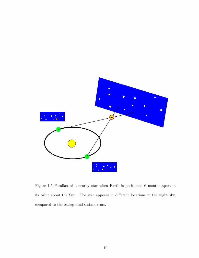
Figure 1.5 Parallax of a nearby star when Earth is positioned 6 months apart in
its orbit about the Sun. The star appears in different locations in the night sky,
compared to the background distant stars.
10

dim a bright object, like a lighthouse flame far from the shore. If the exact brightness
of a far away object is known, a distance could be estimated from the brightness
observed.
1.2.2 Hipparcus, Magnitude Scale and Distance Modulus
The only data we receive from stellar objects is light and on Earth we receive
only a small portion of the electromagnetic spectrum. The ancient Greek astronomer
Hipparcus first divided the brightness of stars into six classes; the brightest ones
being Class-1 and the faintest being Class-6. This is the basis of the magnitude scale
astronomers currently use
m = −2.5logf
f0= −2.5log
L
4πd2+ C (1.2)
where m is an apparent magnitude or brightness seen from Earth, d is the distance
from Earth, f is the observed flux, and f0 is reference flux (such as for the star
Vega). This definition of magnitude continues Hipparcus’ system of stellar objects
being assigned larger magnitude values while having a dimmer brightness.
The absolute magnitude, M, is a measure of the true brightness of the star. Cur-
rently, the scale of apparent magnitude goes into the negatives with the Sun at -26.74
and the extremely dim 26 magnitudes, which are discussed in this study of GCs sur-
rounding NGC1533 and the 11 Shapley Supercluster galaxies. Galaxy magnitudes
and globular cluster magnitudes use the same stellar magnitude scale. Our study
uses the powerful Hubble Space Telescope to obtain images that can be analyzed to
get magnitudes for globular clusters well beyond our own galaxy and will be discussed
in the following sections. A distance can be calculated if the apparent magnitude is
measured and if the absolute magnitude is known. The absolute magnitude is defined
as the apparent magnitude that the object would have if it were at a distance of 10
pc. This relation can be written in the following equation,
M = −2.5 logL
4π102+ C (1.3)
11

where this is the apparent magnitude equation with d = 10 pc.
For galaxies, which have diameters much greater than 10 pc, the absolute magni-
tude is that of a star of same luminosity as the whole galaxy. The difference between
the apparent magnitude, m, and the absolute magnitude, M, is called the distance
modulus.
distance modulus = m − M (1.4)
The distance modulus or DM can be used to find the distance to the object by
combining equations 1.2 and 1.3 the following way,
DM = m − M = 2.5logd2
102= 5 ∗ log
d
10pc(1.5)
where d is the distance measured in pc.
1.2.3 Filters and Color
Keep in mind that the value for magnitude will differ with the filter or bandpass
used to image the light from a star or galaxy. The filter allows only certain wavelengths
to pass and be collected. Common filters, that limit these ranges, in astronomy are
the UBVRI bands, which is the Johnson system which designates U for ultraviolet
and I for infrared, with BVR covering blue, visible, and red, respectively. There are
many more filters used by astronomical instruments which cover other wavelengths
in the electromagnetic spectrum. The magnitude taken in the B band is called mB
or just B. Taking the difference between magnitudes taken in two different filters is
called a color; B - V is the color from the difference in mB - mV = MB - MV , since
the absolute magnitude is just a shift of the apparent magnitude.
1.2.4 Standard Candles
If the absolute magnitude is known (or is estimated from assumptions), that class
of object is called a standard candle. An example of a standard candle is a vari-
able star, which is a star whose brightness changes in a periodic fashion. Variable
12
stars close enough to get a distance measurement using parallax were discovered by
Henrietta Swan Leavitt to have a correlation between the period of variation and
the luminosity. There are several classifications of variable stars that follow different
period-luminosity relations, such as type I and II Cepheid variables and RR Lyrae
stars. The assumption that all variable stars follow the same period-luminosity re-
lation was the reason Shapley’s distance measurements were not as accurate as they
could have been. However, Cepheid variables played a major role in finding accurate
distances to globular clusters and in turn the location of our solar system within the
Milky Way.
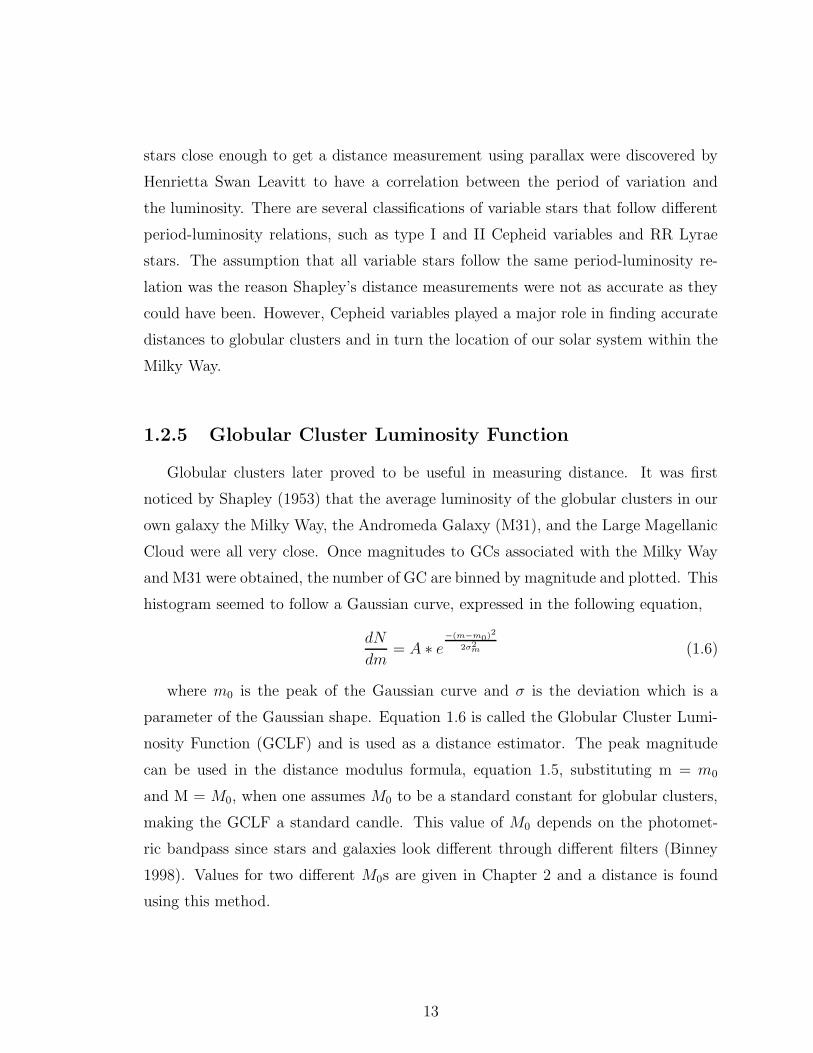
1.2.5 Globular Cluster Luminosity Function
Globular clusters later proved to be useful in measuring distance. It was first
noticed by Shapley (1953) that the average luminosity of the globular clusters in our
own galaxy the Milky Way, the Andromeda Galaxy (M31), and the Large Magellanic
Cloud were all very close. Once magnitudes to GCs associated with the Milky Way
and M31 were obtained, the number of GC are binned by magnitude and plotted. This
histogram seemed to follow a Gaussian curve, expressed in the following equation,
dN
dm= A ∗ e
−(m−m0)2
2σ2m (1.6)
where m0 is the peak of the Gaussian curve and σ is the deviation which is a
parameter of the Gaussian shape. Equation 1.6 is called the Globular Cluster Lumi-
nosity Function (GCLF) and is used as a distance estimator. The peak magnitude
can be used in the distance modulus formula, equation 1.5, substituting m = m0
and M = M0, when one assumes M0 to be a standard constant for globular clusters,
making the GCLF a standard candle. This value of M0 depends on the photomet-
ric bandpass since stars and galaxies look different through different filters (Binney
1998). Values for two different M0s are given in Chapter 2 and a distance is found
using this method.
13
1.2.6 Surface Brightness Fluctuation
Another indirect distance method used in Chapter 2 to obtain a distance to
NGC1533 uses surface brightness fluctuations of the stellar object and is called the
SBF method. This method takes advantage of the CCD camera, described in the
next section, and the graininess of the image and was first described in Tonry and
Schneider (1988). Since a galaxy is made up of individual stars, the graininess or
surface brightness fluctuation is directly proportional to its distance. Using models
of a galaxy made up of N number of stars and a Poisson distribution,√
N for any
portion of the galaxy, we can relate variations in brightness to distance. If a galaxy
is at double the distance, the variance will fall by 1/4. The CCD camera helps get a
more accurate measure of the galaxy’s brightness variation by being able to measure
number and luminosity of each star that falls into individual pixels within the image.
1.2.7 GC Size
This method is based on the assumption that the median half-light radius, a size
measurement that corresponds to the radius from the core that contains half the total
mass, of globular clusters surrounding a galaxy is constant. This method is used in
Chapter 2 and assumes this mean size is about 3 pc, which was derived from a Virgo
cluster survey discussed in Jordan et al. (2005). Once the GC sizes are measured
from an image, the median size can be used in the following equation,
d =0.552 ± 0.058
〈rh〉Mpc, (1.7)
where 〈rh〉 is the corrected median half-light radius in arcseconds. This method is a
good estimate but is not as accurate as SBF or GCLF measurements.
1.2.8 Redshift and Hubble’s Law
The subject of cosmology is too large of a subject to be explained in a small
section. However, I will briefly try to discuss the motions of galaxies in our universe
and how those motions relate to distance from Earth.
14
In 1914, Vesto Slipher first published the observation that almost all galaxies had
spectral lines that were systematically shifted to the red. This observation suggests
that the galaxies with “redshifted” spectral lines are all traveling away from the Milky
Way. Edwin Hubble investigated this phenomena and found a relation between the
shift and the galaxy’s distance from Earth. The redshift, z, can be used to find
distance the following way,
d =cz
H0
Mpc, (1.8)
where d is distance, c is the speed of light (3×10⁵ km/s), z � 1 and H0 is the
Hubble constant. The Hubble constant currently ranges from 70-75 km/s−1 Mpc−1,
depending on what study is used and error (73.8 ± 2.4, Riess et al. 2011 and 72.6 ±3.1 Suyu et al. 2010). The value cz (speed of light × redshift) represents the recession
velocity of the galaxy.
This discovery gave way to the notion that the Universe is expanding, which is
described by Hubble’s Law. The source of these velocities is what astronomers call the
Big Bang event. The Big Bang theory describes the universe initially concentrated
in extremely small size scale which began to expand rapidly. This expansion is also
called the Hubble Flow.
1.3 Galaxy Types
In this globular cluster study, the host galaxies NGC1533 and the 11 Shapley
Supercluster galaxies are various kinds of Elliptical galaxies (E) and an S0 galaxy.
To better understand what those galaxy classifications mean and how they further
relate to formation scenarios, a list and description of various classification types is
discussed below. However, we must keep in mind that the appearance of a galaxy or
cluster can vary greatly depending on which wavelength or filter in which it is being
viewed.
15
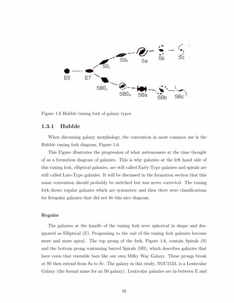
Figure 1.6 Hubble tuning fork of galaxy types
1.3.1 Hubble
When discussing galaxy morphology, the convention in most common use is the
Hubble tuning fork diagram, Figure 1.6.
This Figure illustrates the progression of what astronomers at the time thought
of as a formation diagram of galaxies. This is why galaxies at the left hand side of
this tuning fork, elliptical galaxies, are still called Early-Type galaxies and spirals are
still called Late-Type galaxies. It will be discussed in the formation section that this
name convention should probably be switched but was never corrected. The tuning
fork shows regular galaxies which are symmetric and then there were classifications
for Irregular galaxies that did not fit this nice diagram.
Regular
The galaxies at the handle of the tuning fork were spherical in shape and des-
ignated as Elliptical (E). Progressing to the end of the tuning fork galaxies become
more and more spiral. The top prong of the fork, Figure 1.6, contain Spirals (S)
and the bottom prong containing barred Spirals (SB), which describes galaxies that
have cores that resemble bars like our own Milky Way Galaxy. These prongs break
at S0 then extend from Sa to Sc. The galaxy in this study, NGC1533, is a Lenticular
Galaxy (the formal name for an S0 galaxy). Lenticular galaxies are in-between E and
16

S. The galaxies in the Shapley Supercluster study are all elliptical.
Irregular
When a galaxy is asymmetrical it is called Irregular, (Irr). There were two types
of Irregular galaxy in the Hubble classification scheme (not displayed on the fork).
The Irr I galaxies are asymmetrical, without well defined spiral arms and contain
knots of young, hot stars. The Irr II galaxies are smooth, asymmetrical galaxies.
de Vaucouleurs
In the 1950s astronomer Gerard de Vaucouleurs felt that the Hubble sequence did
not take into account the wide variations of galaxies and extended the prongs in the
Hubble tuning fork with another Sd galaxy and renamed the Irregular classifications.
He also restricted the definition of Lenticular Galaxy, S0, as a galaxy that could not
be confirmed to have a bar. The de Vaucouleurs classification is seen as a modified
Hubble classification.
1.3.2 Dwarfs and cD galaxies
Elliptical galaxies with low luminosity are called dwarf elliptical galaxies (dE).
The other end of the size spectrum contains the central dominated galaxy or cD
galaxy. This classification is from the Yerkes classification scheme but seems to pop
up whenever a giant elliptical at the center of a cluster is being described. The
definition of a cD galaxy is a galaxy whose light profile falls by R1/4, where R is the
radius from the galaxy center. Most of the galaxies that dominate a cluster are cD
galaxies.
17
1.4 Cluster Types
Just like galaxies, the clusters in which the galaxies reside are also grouped into
types. The most basic classification is describing clusters as rich or poor clusters.
This description directly relates to the number and density of galaxies within a clus-
ter, cluster members. Also, the classification of regular and irregular referring to
symmetry of the object applies to clusters just as it applied to galaxies.
1.4.1 Bautz-Morgan type
This cluster type was developed by astronomers Laura Bautz and William Wilson
Morgan in 1970 to describe the kind of members a cluster possesses. If a cluster is
dominated by a cD galaxy larger than the other cluster members, it is designated
with a Bautz-Morgan(BM) type I. A cluster with many members having similar sizes
and luminosities, with no dominating galaxy, was given a BM type III. BM types of
I-II, II, and II-III were given to clusters that exhibited a morphology between these
two extremes.
1.4.2 Rood-Sastry type
This cluster classification scheme is much like the Hubble galaxy classification
since it utilizes the tuning fork. Rood-Sastry tuning fork was first published in 1971,
Figure 1.7. It is basically the Bautz-Morgan system in fork form and more considera-
tion is given to the locations of the cluster members. A cD cluster has one dominating
bright cD galaxy where the B cluster has two dominant galaxies, binary galaxies. The
fork then splits into two prongs with L clusters and C clusters. The L (linear) clusters
have some of the brightest galaxies arranged in a line and the C cluster with bright-
est members concentrated toward the center. The fork ends with the F cluster and I
cluster. The F cluster has galaxies distributed in a uniform flat manner as opposed
to the I cluster that has an irregular distribution of galaxy members. The problem
with this classification scheme is its high degree of subjectivity.
18
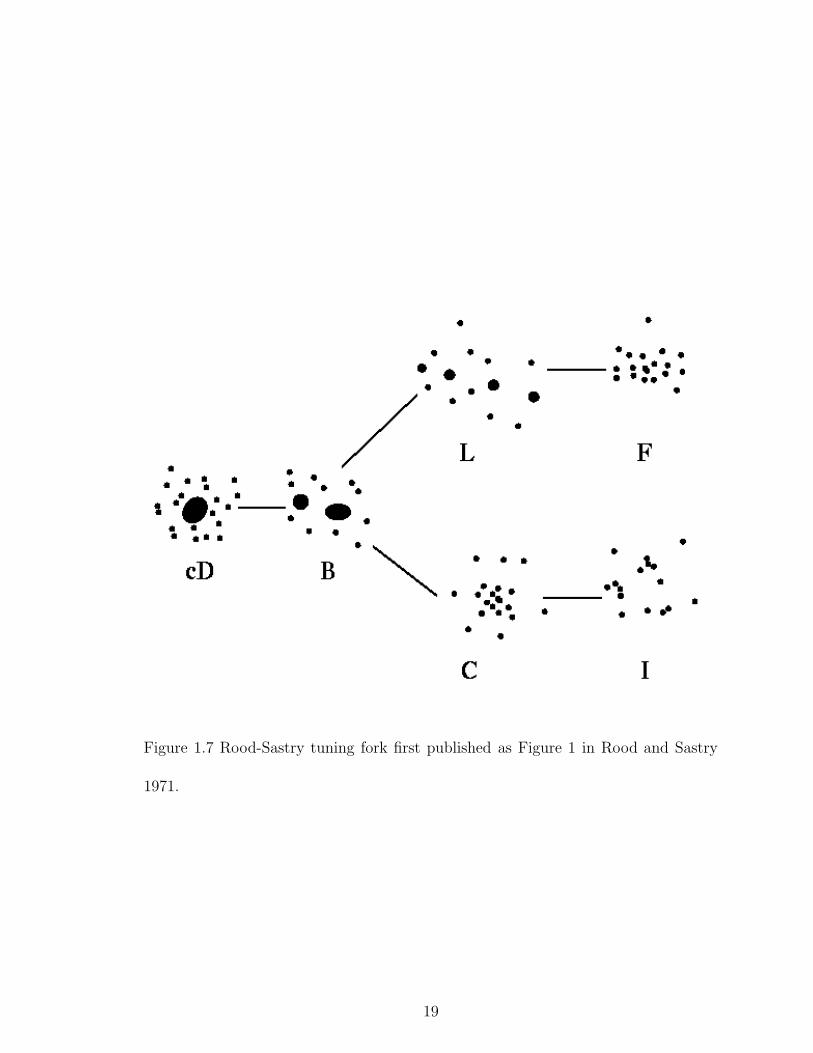
Figure 1.7 Rood-Sastry tuning fork first published as Figure 1 in Rood and Sastry
1971.
19

1.5 Formation Scenarios
A galaxy formation model that describes characteristics, such as globular clusters,
currently does not exist. Although, I will try to summarize astronomy’s best attempt
(Mo, van den Bosch, and White 2010).
1.5.1 Old Thought
The first idea that tried to describe galaxy formation can be summed up in one
word: Gravity. First let us start with spiral disk galaxies like the Milky Way. Collapse
of a gas cloud, due to gravity caused by a large amount of mass, with some initial
angular momentum may eventually flatten the cloud and star formation is ignited
with the collapse. This explanation is entirely too simple since we are really dealing
with a many body problem due to the number of stars that build a galaxy and we
know that many body problems are extremely difficult. However, let us go with it for
now and consider elliptical galaxies. To describe the formation of elliptical galaxies,
such as the bulk of the type of galaxy in this study, we can consider two possibilities:
mergers and monolithic collapse.
Merger
A scenario where the formation of an elliptical galaxy is a result of two or more
merging spirals is one attempt to explain elliptical galaxy formation. This process
would mean that the notion that the Hubble tuning fork, Figure 1.6, shows galaxy
evolution as false unless you start at the prong end of the fork. In this scenario the
star formation occurs before the merger, within the spiral galaxies, and the stars
are just reassembled in the interaction of the merging spirals to create the elliptical
galaxy.
20

Monolithic Collapse
This scenario requires a quick collapse of the gas cloud to create an elliptical
galaxy. If the star formation occurs relatively quickly compared to the free-fall time
scale, then the collapse will dissipate little or no energy. A single burst of star
formation can be used to explain the homogeneous class that elliptical galaxies seem
to be. However, this scenario does not explain what initial conditions are needed to
create such an event.
1.5.2 New Thought and Dark Matter
It turns out the neither the merger scenario nor the monolithic collapse scenario
can fully explain our observations of galaxy morphology. Computer simulations fail at
reproducing galaxies as we see them today by just using a luminosity-mass relation.
Assuming that most of the mass in galaxies is from stars, we can estimate the mass
of each galaxy observed. However, when mass is increased well past the value that is
derived from the galaxy brightness, the end result from simulations start to resemble
the galaxies that can are seen in the sky. So where is this extra mass coming from?
Well, we do not know but we can name it. Scientists have used their collective
imagination and dubbed this mystery non-visible mass source, dark matter. The
model where galaxies are surrounded by a dark matter halo is successfully used in
computer simulations trying to produce an elliptical galaxy by merging two spirals
(Cox et al. 2006) and even can be matched up with images taken by HST, displayed
in a public press release, and shown in Figure 1.8.
It turns out that the differences between the Merger and Monolithic Collapse
scenarios may not make them mutually exclusive. As seen in Figure 1.8, mergers
and interaction happen in the universe. Also, the majority of the stellar populations
of ellipticals have been found to be old which supports the notion of major star
forming events. The attempt to create models with younger stellar ages has failed to
reproduce results that resemble the ellipticals we observe (Renzini 2006). The more
likely hierarchical merger of galaxies, to produce an elliptical galaxy along with star
21
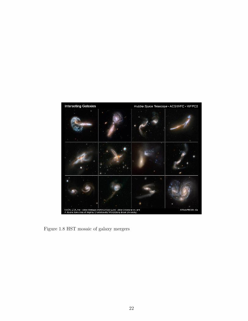
Figure 1.8 HST mosaic of galaxy mergers
22
formation during the interaction, is the accepted theory to date.
1.6 The CCD and the Hubble Space Telescope
The CCD camera and Hubble Space Telescope (HST) have contributed to recent
breakthroughs in the study of globular clusters. However, before I describe these
breakthroughs I will first describe the instrument that has changed the landscape of
astronomy. The CCD or Charged Coupled Device is used to electronically record light
signals. CCDs have a much greater efficiency than photographic plates. CCDs are
cooled with liquid nitrogen or electrically to reduce thermal noise, and the data are
digitally transferred. Efficiency in photon detection reduces the number of exposures
needed to match the quality of images taken with a photographic plate. The CCD
consists of an array of capacitors on a semiconductor substrate. The capacitors store
the charge or data that is transferred and the semiconductor is the photo-active region
that detects the photons.
Since the 1920s, astronomers hoped it would be possible to orbit giant telescopes
around the Earth. A space telescope takes advantage of the absence of atmosphere.
It was discovered very early in astronomy that the atmosphere blocked certain wave-
lengths, and created the twinkling effect of stars. The Hubble Space Telescope was
launched into orbit in 1990. HST has a 2.4 meter mirror and is equipped with cameras
and spectrometers, which detect data in the visual, near IR and near UV spectrum,
as the instruments in Figure 1.9. Initially it was discovered that the HST mirror
had a defect. Once it was corrected in 1993, HST has been supplying the scientific
community with the most detailed images, in this spectral regime, ever produced
of galaxy cores, supernovae, globular clusters and many more stellar objects. This
wealth of data has contributed to the advancement in the areas of stellar and galactic
evolution and cosmology, directly and indirectly.
The instruments aboard HST have changed over the years so that the most ad-
vanced cameras could be utilized as well as replacing instruments that have run their
life expectancy in space. One current instrument, nearing its own end of operation,
23

Figure 1.9 A simple diagram of the Hubble Space Telescope initially equipped with two
cameras and two spectrometers in the instrument region, courtesy of NASA/STSCI.
24
is the Advanced Camera for Surveys. This is the camera that was used in each of the
projects discussed in this thesis. It images objects in optical wavelengths and will be
revisited in following chapters, along with its specific filters (Binney 1998).
1.7 Globular Cluster Characteristics
Now that we have covered a brief history of globular clusters, classification, evo-
lution and astronomical instruments, we can finally dive into the topics that affect
current GC studies. Here we detail a few of these topics which astronomers feel may
be clues to the mystery of GC evolution: color bimodality of GC populations and
specific frequency of host galaxies.
1.7.1 Color Bimodality
Images can be taken in a variety of wavelengths and as stated above, the difference
in magnitude is called color. When the bandpasses are significantly separated in
wavelength, it has been seen that globular cluster populations around galaxies have
been found to be bimodal. It seems that when a histogram is created with number
of galaxies verses color magnitude bins, two peaks become present. However, since
globular clusters are thought to be objects that differ little from host galaxy to host
galaxy as well as lacking in complexity due to the stellar population of a globular
cluster being homogeneous, color bimodality was concluded to be directly related to
metallicity. Metallicity is the relative chemical abundance of iron with respect to
hydrogen, [Fe/H]. The assumption that color and metallicity are directly related is
further investigated in Chapter 6. The Milky Way GC population has been known to
be bimodal for some time and spectroscopy of these globular clusters has shown that
the two subpopulations do indeed differ in metallicity. A current review on globular
clusters by Brodie & Strader (2006) makes the bold claim that this phenomena is
prominent with ellipticals as host galaxies, so much so that “no massive elliptical (E)
galaxy has been convincingly shown to lack GC subpopulations”. This statement is
25
supported by this thesis.
The seemingly universal occurrence of bimodality of GC populations in ellipticals
seems to hint at galaxy evolution. The two current theories that try to explain color
bimodality are different generations of globular clusters or/and mergers. If galaxy
formation occurs in short bursts of stellar formation (monolithic collapse), then the
early one would produce the halo GCs since ages derived for globular clusters are
found to be older then the host galaxies and possible later ones would produce another
subpopulation with higher metal content. In the case of “closed-box” self-enrichment,
the younger a stellar object is the more metal rich it is due to supernovae as the
main mechanism that creates these heavier metals. The second theory of dry merger
(merger scenario in galaxy formation) claims that GC populations that halo two or
more different galaxies with different metallicities merge to create one galaxy with
two color subpopulations of globular clusters. The most likely scenario being one
giant galaxy with a red population of GCs merging with many smaller galaxies with
blue GC populations.
These two theories have problems matching the observations. One problem with
the different generation theory comes from recent studies finding that most GC sub-
populations that show color bimodality do not have the age difference required to
explain the metallicity bimodality (Chies-Santos et al. 2011). One problem with the
dry merger scenario is that it relies too heavily on low mass objects to make the large
galaxies that are observed (West et al. 2004). Also, why do these massive ellipticals
more than often have only two subpopulations? If there are more than one interac-
tion in creating a galaxy then there would also be more occurrences of more than two
subpopulations.
The statement that all massive ellipticals show subpopulations is further investi-
gated in this study by supplying more data. We also consider the assumption of the
direct link between color and metallicity.
26
1.7.2 Specific Frequency
The notion that globular cluster evolution is intertwined with the evolution of
its host galaxy is extended in the concept of Specific Frequency, SN . If the stellar
components of a galaxy contribute to its luminosity, then the number of GC should
directly relate to the magnitude of the host galaxy in the visible band, MV . The
mathematical definition of SN is,
SN = Ntot10−0.4(MV +15) (1.9)
where Ntot is the total number of GCs associated with the host galaxy. This equation
is normalized to the specific frequency of the Milky Way. If ellipticals are born from
a merger of two spirals, then the specific frequency of that elliptical would equal that
of the SN of the spirals since the birth was created through dry mergers. SN values
for most spirals are found to be 1-2 and the values of ellipticals have a large range
from 2-20. The range seems to sometimes result from distance a host galaxy is to its
cluster’s center. This is found in this study as well as in Blakeslee and Tonry (1995).
Therefore, an investigation into SN values can give insight into galactic evolution.
In this study specific frequency is calculated for all galaxies. We consider the
notion that globular clusters might be taken or added to host galaxies in mergers
and may be associated with the cluster of galaxies as opposed to the host galaxy, as
previously thought.
1.8 Thesis Outline
Chapter 2, details a study done on the GC system of NGC1533, a S0 galaxy
with star formation in its outer regions. In the following chapter, chapter 3, we will
investigate new stellar objects currently named Ultra Compact Dwarfs, which are
another subpopulation with sizes larger than GCs and smaller than dwarf galaxies.
This study is on the UCD population of Shapley Supercluster galaxy in AS0740,
ESO325-G004. Chapters 2 and 3 both describe published work and the chapters are
27
basically the corresponding published papers. Chapter 4 describes the data analysis
on the one-band imaging GC study done on the 11 Shapley Supercluster galaxies.
This chapter also includes a brief introduction to the Shapley Supercluser and the
motivations for obtaining the data. The results from this F814W band study and
conclusions reside in Chapter 5. Chapter 6 is a revisit to the special galaxy in our
Shapley survey, ESO325-G004 and its GC population. Using the two additional filters
we were able to use results from Chapter 5 and further investigate the GC population
with color data. We conclude with a summary of these three projects and future
related work in Chapter 7.
28

Bibliography
[1] Bautz, L. P., & Morgan, W. W. 1970, ApJ, 162, L149
[7] Binney, J., & Merrifield, M. 1998, Galactic astronomy / James Binney and Michael
Merrifield. Princeton, NJ : Princeton University Press, 1998. (Princeton series in
astrophysics) QB857 .B522 1998
[3] Blakeslee, J. P., et al. 2010, ApJ, 724, 657
[2] Blakeslee, J. P., & Tonry, J. L. 1995, ApJ, 442, 579
[6] Brodie, J. P., & Strader, J. 2006, ARA&A, 44, 193
[10] Chies-Santos, A. L., Larsen, S. S., Kuntschner, H., Anders, P., Wehner, E. M.,
Strader, J., Brodie, J. P., & Santos, J. F. C. 2011, A&A, 525, A20
[7] Cox, T. J., Di Matteo, T., Hernquist, L., Hopkins, P. F., Robertson, B., &
Springel, V. 2006, ApJ, 643, 692
[23] Curtis, H., 1921, The Scale of the Universe, Bull. Nat. Res. Counc., 2, part 3,
194-217
[10] Harris, W. E., & van den Bergh, S. 1981, AJ, 86, 1627
[10] Herschel, W. 1785, Royal Society of London Philosophical Transactions Series I,
75, 213
[11] Hubble, E. 1929, Proceedings of the National Academy of Science, 15, 168
29

[29] Jordan, A., et al. 2005, ApJ, 634, 1002
[13] Kant, I. 1755, Zeitz, Bei W. Webel, 1798. Neue aufl.,
[23] Messsier, Charles, Catalogue des Nbuleuses & des amas d’toiles. Connoissance
des Temps for 1784 (published 1781) pp. 227-267 [Bibcode: 1781CdT..1784..227M]
[19] Mo, H., van den Bosch, F. C., & White, S. 2010, Galaxy Formation and Evolution
by Houjun Mo, Frank van den Bosch and Simon White. Cambridge University
Press, 2010. ISBN: 9780521857932,
[16] Piotto, G., et al. 2007, ApJ, 661, L53
[17] Renzini, A. 2006, ARA&A, 44, 141
[18] Riess, A. G., et al. 2011, ApJ, 730, 119
[19] Rood, H. J., & Sastry, G. N. 1971, PASP, 83, 313
[20] Seeds, M. A. 1998, Horizons : exploring the universe / Michael A. Seeds. Bel-
mont, CA : Wadsworth Pub. Co., c1998. QB45 .S44 1998
[21] Shapley, H. 1918, PASP, 30, 42
[23] Shapley, H., 1921, The Scale of the Universe, Bull. Nat. Res. Counc., 2, part 3,
171-193
[23] Shapley, H.,1953, Proc. Nat. Acad. Sci. (Wash), 39, 349.
[24] Slipher, V. M. 1914, Lowell Observatory Bulletin, 2, 66
[25] Suyu, S. H., Marshall, P. J., Auger, M. W., Hilbert, S., Blandford, R. D., Koop-
mans, L. V. E., Fassnacht, C. D., & Treu, T. 2010, ApJ, 711, 201
[26] Tonry, J., & Schneider, D. P. 1988, AJ, 96, 807
[27] West, M. J., Cote, P., Marzke, R. O., & Jordan, A. 2004, Nature, 427, 31
30

Chapter 2
Structure, Globular Clusters, and
Distance of the Star-Forming S0
Galaxy NGC 1533 in Dorado
This chapter was published under the same title in The Astrophysical Journal, Vol.
371, Issue 2, pp 1624-1639 (2007). The work presented in Chapter 2 was undertaken
in collaboration with Dr. John Blakeslee, who completed the data analysis in sections
3 and 4.
Synopsis
We use two-band imaging data from the Advanced Camera for Surveys on board
the Hubble Space Telescope for a detailed study of NGC1533, an SB0 galaxy in the
Dorado group surrounded by a partial ring of H I. NGC1533 appears to be completing
a transition from late to early type: it is red, but not quite dead. Faint spiral structure
31

becomes visible following galaxy subtraction, and luminous blue stars can be seen in
isolated areas of the disk. Dust is visible in the color map in the region around
the bar, and there is a linear color gradient throughout the disk. We determine
an accurate distance from the surface brightness fluctuations (SBF) method, finding
(m−M) = 31.44 ± 0.12 mag, or d = 19.4 ± 1.1 Mpc. We then study the globular
cluster (GC) colors, sizes, and luminosity function (GCLF). Estimates of the distance
from the median of the GC half-light radii and from the peak of the GCLF both agree
well with the SBF distance. The GC specific frequency is SN = 1.3±0.2, typical for an
early-type disk galaxy. The color distribution is bimodal, as commonly observed for
bright galaxies. There is a suggestion of the redder GCs having smaller sizes, but the
trend is not significant. The sizes do increase significantly with galactocentric radius,
in a manner more similar to the Milky Way GC system than to those in Virgo. This
difference may be an effect of the steeper density gradients in loose groups. Additional
studies of early-type galaxies in low density regions can help determine if this is indeed
a general environmental trend.
2.1 Introduction
The Hubble Space Telescope (HST) has opened the door to our understanding
of extragalactic star cluster systems, revealing numerous globular clusters (GCs) in
early-type galaxies (e.g. Gebhardt & Kisler-Patig, 1999; Peng et al. 2006) as well as
“super-star clusters” (SSCs) in late-type galaxies (Larsen & Richtler 2000), especially
starbursts (e.g. Meurer et al. 1995, Maoz et al. 1996). In early-type systems the color
distribution of the GCs is often bimodal, consisting of a blue metal-poor component
and a red metal-rich component (e.g. West et al. 2004; Peng et al. 2006). This
observation gives a hint to the connection between the early- and late-type systems.
Mergers often have particularly strong starbursts and rich populations of SSCs, as
seen for example in NGC4038/39 - “the Antennae” system (Whitmore & Schweizer
1995; Whitmore et al. 1999), and this is one possible origin for the redder population
of GCs in early-type galaxies (e.g., Ashman & Zepf 1998).
32
Much of the research on GC systems has concentrated on galaxy clusters which
are rich in early-type galaxies (e.g., the ACS Virgo Cluster Survey, Cote et al. 2004;
the ACS Fornax Cluster Survey, Jordan et al. 2007). Early-type galaxies in groups
and the field are somewhat less studied, particularly with HST and the Wide Field
Channel (WFC) of its Advanced Camera for Surveys (ACS). The relatively wide
(3.′4) field of view of the ACS WFC combined with its fine pixel sampling make it an
exceptional tool for imaging GCs out to a few tens of Mpc where they have measurable
angular sizes (Jordan et al. 2005).
Here we report HST ACS/WFC imaging of the SB0 (barred lenticular) galaxy
NGC 1533 in the Dorado group. This group is in the “Fornax wall” (Kilborn et al.
2005) and hence at a similar distance to the Fornax cluster (e.g., Tonry et al. 2001).
Dorado is interesting in that it is richer than the Local Group but still dominated by
disk galaxies (its brightest members being the spiral NGC 1566 and the S0 NGC 1553),
and its members have H I masses similar to non-interacting galaxies with the same
morphology (Kilborn et al. 2005). While the apparent crossing time of the group is
only ∼ 13% of the age of the universe (Firth et al. 2006; see also Ferguson & Sandage
1990), the most recent analyses conclude the group is unvirialized (Kilborn et al.
2005; Firth et al. 2006), which may explain the richness in spirals and H I.
NGC 1533 is the seventh brightest member of the Dorado group. It lies within the
virial radius, but is a ∼ 2-σ velocity outlier (Kilborn et al., 2005; Firth et al. 2006) so
that it is moving at high speed through the intra-group medium. A vast H I arc is seen
in the outskirts of NGC 1533 and is connected to its Sdm companion IC 2038 (Ryan-
Weber et al. 2004), suggesting that NGC 1533 is “stealing” ISM from its companion.
As is typically seen in S0 galaxies, star formation is weak in NGC 1533. Observations
of this galaxy in spectroscopic surveys note the presence of emission lines (Jorgensen
et al. 1997; Bernardi et al. 2002); the nuclear spectrum available from the 6dF survey
(Jones et al. 2005) shows [N ii]6584 and weak Hα. Hα imaging from the Survey of
Ionization in Neutral Gas Galaxies (SINGG, an Hα imaging survey of H I selected
galaxies; Meurer et al. 2006) shows a few weak H II regions beyond the end of its
bar (the nucleus is too bright to allow faint nuclear H II regions to be detected in
the SINGG images), as well as a scattering of very faint “intergalactic H II regions”.
33
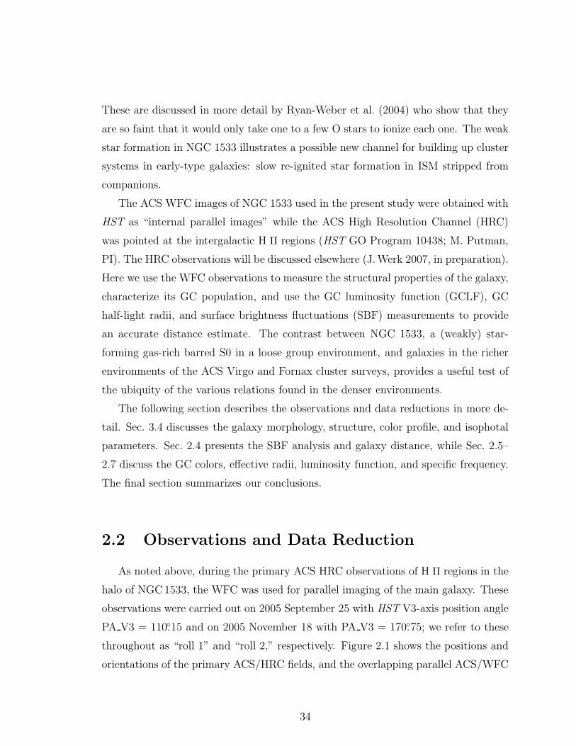
These are discussed in more detail by Ryan-Weber et al. (2004) who show that they
are so faint that it would only take one to a few O stars to ionize each one. The weak
star formation in NGC 1533 illustrates a possible new channel for building up cluster
systems in early-type galaxies: slow re-ignited star formation in ISM stripped from
companions.
The ACS WFC images of NGC 1533 used in the present study were obtained with
HST as “internal parallel images” while the ACS High Resolution Channel (HRC)
was pointed at the intergalactic H II regions (HST GO Program 10438; M. Putman,
PI). The HRC observations will be discussed elsewhere (J.Werk 2007, in preparation).
Here we use the WFC observations to measure the structural properties of the galaxy,
characterize its GC population, and use the GC luminosity function (GCLF), GC
half-light radii, and surface brightness fluctuations (SBF) measurements to provide
an accurate distance estimate. The contrast between NGC 1533, a (weakly) star-
forming gas-rich barred S0 in a loose group environment, and galaxies in the richer
environments of the ACS Virgo and Fornax cluster surveys, provides a useful test of
the ubiquity of the various relations found in the denser environments.
The following section describes the observations and data reductions in more de-
tail. Sec. 3.4 discusses the galaxy morphology, structure, color profile, and isophotal
parameters. Sec. 2.4 presents the SBF analysis and galaxy distance, while Sec. 2.5–
2.7 discuss the GC colors, effective radii, luminosity function, and specific frequency.
The final section summarizes our conclusions.
2.2 Observations and Data Reduction
As noted above, during the primary ACS HRC observations of H II regions in the
halo of NGC1533, the WFC was used for parallel imaging of the main galaxy. These
observations were carried out on 2005 September 25 with HST V3-axis position angle
PA V3 = 110.◦15 and on 2005 November 18 with PA V3 = 170.◦75; we refer to these
throughout as “roll 1” and “roll 2,” respectively. Figure 2.1 shows the positions and
orientations of the primary ACS/HRC fields, and the overlapping parallel ACS/WFC
34
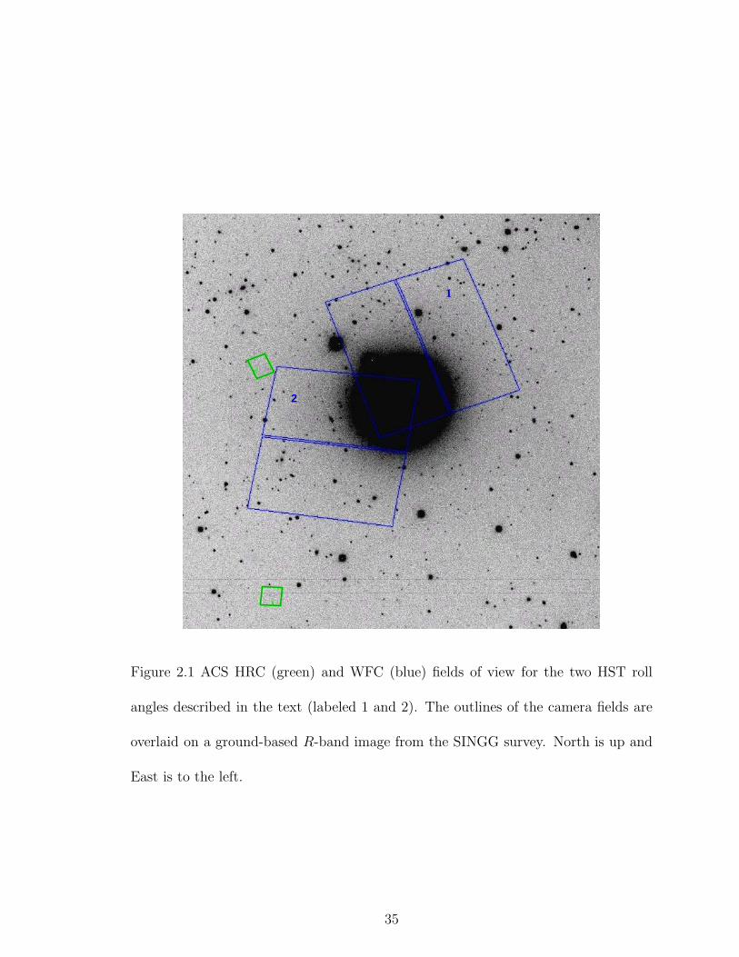
1
2
Figure 2.1 ACS HRC (green) and WFC (blue) fields of view for the two HST roll
angles described in the text (labeled 1 and 2). The outlines of the camera fields are
overlaid on a ground-based R-band image from the SINGG survey. North is up and
East is to the left.
35
fields, at the two roll angles.
2.2.1 Image Processing
NGC 1533 was imaged in the F814W and F606W bandpasses of the ACS/WFC.
Eight exposures totaling 4950 s in F814W, and four exposures totalling 1144 s in
F606W, were taken at each of the two roll angles. Following standard calibration
by the STScI archive, the data were processed with the ACS IDT “Apsis” pipeline
(Blakeslee et al. 2003) to produce final, geometrically corrected, cleaned images with
units of accumulated electrons per pixel. Apsis also ensures the different bandpass
images are aligned to better than 0.1 pix and performs automatic astrometric recali-
bration of the processed images.
We calibrated the photometry using the Vega-based m1 zero points from Sirianni
et al. (2005): m1, F606 = 26.398 and m1, F814 = 25.501. Galactic extinction was taken
into account using the dust maps of Schlegel et al. (1998) and the extinction ratios
from Sirianni et al. (2005). We determined corrections of A606 = 0.045 mag and
A814 = 0.029 mag for the F606W and F814W bandpasses, respectively. For compar-
ison to other studies, we also converted the measured (F606W−F814W) colors to
Johnson–Cousins (V −I) using the empirically-based prescription given by Sirianni
et al.
We processed the data at the two roll angles with Apsis both separately and
combined together. The upper left panel of Figure 2.2 shows the result from the
combined processing, which is useful for analyzing the galaxy 2-D surface brightness
distribution and isophotal parameters using the largest angular range. However, for
the SBF and globular cluster analyses, we considered each pointing separately and
then merged the results at the end. This was done to avoid PSF and orientation
mismatch effects (e.g., diffraction spikes and effects due to the gate structure of the
CCDs do not match up when combining images with differing orientations). For
each filter image at each pointing, we modeled the galaxy light using the “elliprof”
software written by J. Tonry for the SBF Survey of Galaxy Distances (Tonry et al.
1997) and described in more detail by Jordan et al. (2004). Saturated areas, bright
36

sources, diffraction spikes, and dusty regions were masked out for a better model fit.
The galaxy model was then subtracted from the image, revealing faint sources and
residual features, including faint spiral structure as discussed in Sec. 3.4.
2.2.2 Object Photometry
Object detection was performed with Sextractor (Bertin & Arnout 1996) using
the galaxy-subtracted image for detection and an RMS image for the weighting. The
RMS image gives the uncertainty per pixel including the effects of instrumental and
photon shot noise, as well as the additional “noise” from the galaxy surface brightness
fluctuations. It is constructed as described in detail by Jordan et al. (2004):
RMS =√
(RMSAp)2 + (KF ∗ model) , (2.1)
where RMSAp is the Apsis RMS image based on the instrumental and shot noise alone
(Blakeslee et al. 2003), model is the galaxy surface brightness model, and KF gives the
ratio of the variance per pixel from SBF, σ2L, to that from photon shot noise from the
galaxy, σ2p. The KF factor depends on the bandpass, exposure time, galaxy distance
(which determines the apparent amplitude of the SBF), and the image resolution; it
can be estimated as
KF =σ2
L
σ2p
=1
p10−0.4(mF−m∗
1,F ) , (2.2)
where m∗1,F = m1,F + 2.5 log(T ), T is the total exposure time, mF is the SBF magni-
tude in the given bandpass, and p is a factor that reduces the SBF variance because
of the smoothing effect of the PSF. We adopt mF814 ≈ 30 for NGC1533 based on the
measurement from Tonry et al. (2001) in the very similar IC bandpass (and confirmed
by our SBF result in Sec 2.4) and assume MF606 − MF814 ≈ 2 based on expectations
from stellar population models (Liu et al. 2000; Blakeslee et al. 2001, Cantiello et al.
2003) to determine mF606. Following Jordan et al. (2004), we convolved simulated
noise images with the ACS PSFs to determine the p factor in Eq. 2.2; thus, we reduced
the variance ratio by 12 for F606W and by 13 for F814W and finally determined the
values KF606 = 1.1 and KF814 = 6.0.
37
E
N
Figure 2.2 Upper left: Combined F814W ACS/WFC image of NGC 1533. Lowerleft: Contour map of a 3.6.′3×4.′0 portion of the image. Contours are plotted in stepsof a factor of two in intensity, with the faintest being at µI = 20.7 mag arcsec−2.Upper right: The image following galaxy model subtraction, showing the faint spiralstructure (the “plume” 2′ north of the galaxy is a ghost image). The same 3.6.′3×4.′0field is shown; the box marks the central 1′. lower right: Colormap of the central 1′
region of NGC1533, with dark indicating red areas and white indicating blue. Thedark spot at center marks the center of the galaxy. Dust can be seen as faint, dark,wispy features. A compact blue star-forming region is visible to the left of the galaxycenter, near the center-left of the map.
38
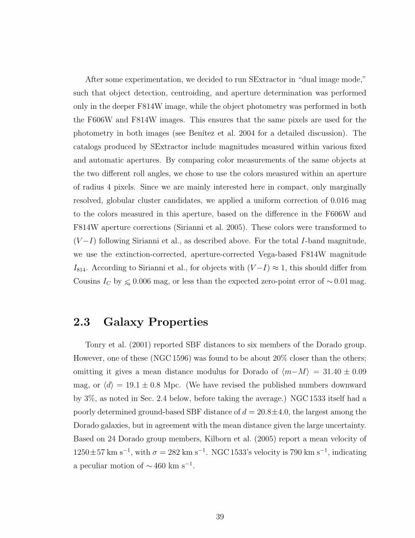
After some experimentation, we decided to run SExtractor in “dual image mode,”
such that object detection, centroiding, and aperture determination was performed
only in the deeper F814W image, while the object photometry was performed in both
the F606W and F814W images. This ensures that the same pixels are used for the
photometry in both images (see Benıtez et al. 2004 for a detailed discussion). The
catalogs produced by SExtractor include magnitudes measured within various fixed
and automatic apertures. By comparing color measurements of the same objects at
the two different roll angles, we chose to use the colors measured within an aperture
of radius 4 pixels. Since we are mainly interested here in compact, only marginally
resolved, globular cluster candidates, we applied a uniform correction of 0.016 mag
to the colors measured in this aperture, based on the difference in the F606W and
F814W aperture corrections (Sirianni et al. 2005). These colors were transformed to
(V −I) following Sirianni et al., as described above. For the total I-band magnitude,
we use the extinction-corrected, aperture-corrected Vega-based F814W magnitude
I814. According to Sirianni et al., for objects with (V −I) ≈ 1, this should differ from
Cousins IC by ∼< 0.006 mag, or less than the expected zero-point error of ∼ 0.01mag.
2.3 Galaxy Properties
Tonry et al. (2001) reported SBF distances to six members of the Dorado group.
However, one of these (NGC1596) was found to be about 20% closer than the others;
omitting it gives a mean distance modulus for Dorado of 〈m−M〉 = 31.40 ± 0.09
mag, or 〈d〉 = 19.1 ± 0.8 Mpc. (We have revised the published numbers downward
by 3%, as noted in Sec. 2.4 below, before taking the average.) NGC1533 itself had a
poorly determined ground-based SBF distance of d = 20.8±4.0, the largest among the
Dorado galaxies, but in agreement with the mean distance given the large uncertainty.
Based on 24 Dorado group members, Kilborn et al. (2005) report a mean velocity of
1250±57 km s−1, with σ = 282 km s−1. NGC1533’s velocity is 790 km s−1, indicating
a peculiar motion of ∼ 460 km s−1.
39
2.3.1 Morphology
The morphological type of NGC 1533 in the RC3 is T = −3 (de Vaucouleurs et al.
1991), indicating an early-type S0. Buta et al. (2006) classify it as (RL)SB00, meaning
that it is a barred, intermediate-type S0 containing both an inner lens structure and
a ring-like feature within the disk. In a morphological study of 15 early-type disk
galaxies, Laurikainen et al. (2006) gives an inner radius of 44′′ for this ring. Some of
these features are evident in the left panels of Figure 2.2. The convex-lens shape of
the outer bulge, the bar, and the disk are clearly seen in the contour map. In addition,
the model-subtracted image in the upper right panel reveals spiral features that are
difficult to see in the original image. The faint spiral arms appear to emanate from
the ends of the bar and wrap around by 360◦. Sandage & Brucato (1979) also noted
a “suggestion of weak spiral pattern in outer lens (or disk)” in NGC1533. It seems
likely that this is the “ring” seen by Buta et al. (2006) and Laurikainen et al. (2006).
Thus, NGC1533 appears to be in the late stages of transition from an early-type
barred spiral to a barred S0 galaxy.
The subtracted image also shows luminous material about 2.′0 to the north/northwest
of the NGC1533 galaxy center, beyond the galaxy disk. This feature is only visible
in the F814W image, not in the F606W or ground-based images. It is apparently an
internal camera reflection from a bright star outside the field of view.
The color map in the lower right panel of Fig. 2.2 reveals the presence of wispy
dust (darker areas in the color map) to the east and south of the nucleus within
the central 20′′ along the bar. Moreover, a compact region of bluer light is visible
at the center left edge of the color map, about 23′′ to the northeast of the galaxy
nucleus. This position coincides with an H II region found by Meurer et al. (2006).
Thus, luminous blue stars are powering the ionization. The areas of dust and star
formation support the view of NGC1533 as a galaxy recently converted from spiral
to S0. However, it should be noted that dust features are found in roughly half of
bright early-type galaxies when studied at high resolution (Ferrarese et al. 2006), and
isolated star formation is not too uncommon.
At larger radius within the disk (outside the color map in the figure), we find
40
several other small groups, or isolated examples, of unresolved blue objects with colors
(V −I) ≈ 0 and magnitudes I814 ∼> 23.5. Some of these are visible in Figure 2.3, and
the ones associated with H II regions are marked in the color-magnitude diagram
presented in Sec. 2.5. They may be a mix of post-asymptotic giant branch (PAGB)
stars, indicating an intermediate age population, and small isolated regions of star
formation. A string of about five such blue objects highlighted in Figure 2.3 are
spread out along one of the spiral arms. The likely connection with the spiral arm in
this case points towards these being a small, dispersed group of fairly young stars.
2.3.2 Galaxy Surface Photometry and Structure
Although NGC1533 has a complex isophotal structure, it can also be enlightening
to study the simple one-dimensional light profile. Figure 2.4 (left panel) shows the
galaxy surface brightness profiles in F606W and F814W. Within a radius of about
16′′, the profile is reasonably well fit by a de Vaucouleurs r1/4-law profile (a straight
line in the figure). Between 16′′ and ∼ 45′′, the profile becomes much flatter; this
includes the inner disk and area around the bar. In the outer disk, beyond ∼ 50′′, the
profile steepens again.
The right panel of Figure 2.4 shows the galaxy color profile. In addition to our
measured (F606W−F814W) profile, we show the ground-based (V −I) photometry
for this galaxy from the Tonry et al. (1997) study (which provides median and average
surface photometry measured in 3′′ radial bins, without removal of external sources).
The ground-based data come from multiple long exposures with the Cerro Tololo 4m
Blanco telescope at a pixel scale of 0.′′47 pix−1. They suffer from poor seeing (1.′′5 in
I, 1.′′8 in V ) and severe central saturation; however, the systematic error on the color
is only 0.018 mag (Tonry et al. 2001). Similar gradients are observed in both sets
of photometry. By binning the data at the same scales and comparing colors over a
radial range of 10′′ – 50′′, we determined:
(V −I)0 = (1.196 ± 0.003) + (1.2 ± 0.2) [(F606W − F814W)0 − 0.95] , (2.3)
with an RMS scatter of 0.010 mag in the fit. This relation yields (V −I) colors be-
41
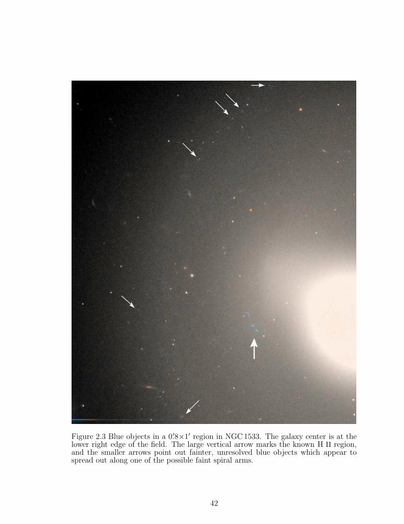
Figure 2.3 Blue objects in a 0.′8×1′ region in NGC1533. The galaxy center is at thelower right edge of the field. The large vertical arrow marks the known H II region,and the smaller arrows point out fainter, unresolved blue objects which appear tospread out along one of the possible faint spiral arms.
42
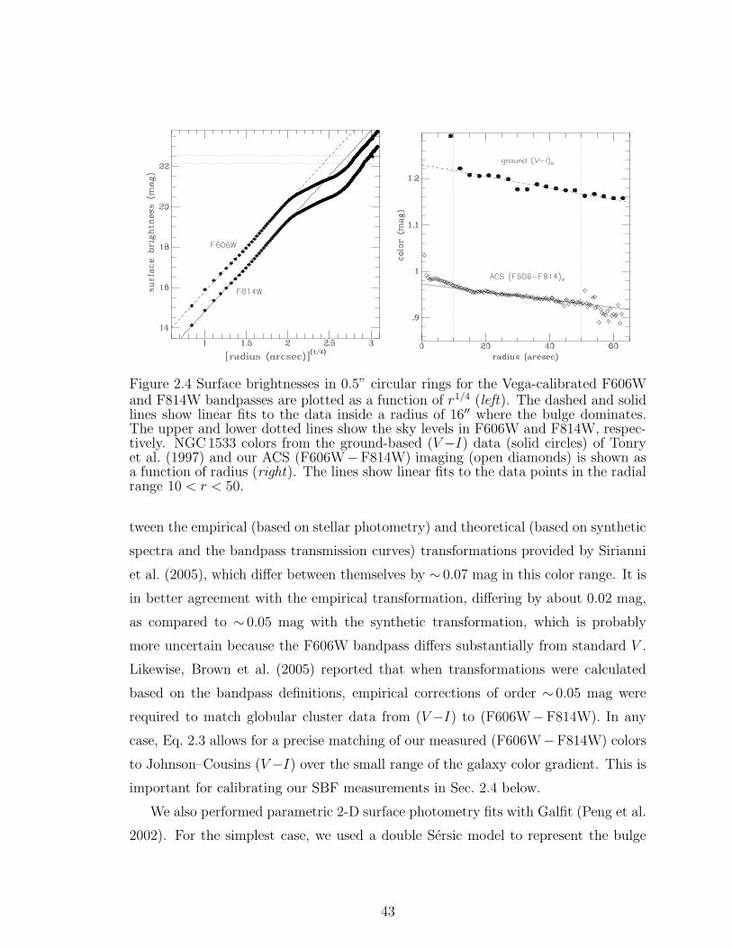
Figure 2.4 Surface brightnesses in 0.5” circular rings for the Vega-calibrated F606Wand F814W bandpasses are plotted as a function of r1/4 (left). The dashed and solidlines show linear fits to the data inside a radius of 16′′ where the bulge dominates.The upper and lower dotted lines show the sky levels in F606W and F814W, respec-tively. NGC1533 colors from the ground-based (V −I) data (solid circles) of Tonryet al. (1997) and our ACS (F606W−F814W) imaging (open diamonds) is shown asa function of radius (right). The lines show linear fits to the data points in the radialrange 10 < r < 50.
tween the empirical (based on stellar photometry) and theoretical (based on synthetic
spectra and the bandpass transmission curves) transformations provided by Sirianni
et al. (2005), which differ between themselves by ∼ 0.07 mag in this color range. It is
in better agreement with the empirical transformation, differing by about 0.02 mag,
as compared to ∼ 0.05 mag with the synthetic transformation, which is probably
more uncertain because the F606W bandpass differs substantially from standard V .
Likewise, Brown et al. (2005) reported that when transformations were calculated
based on the bandpass definitions, empirical corrections of order ∼ 0.05 mag were
required to match globular cluster data from (V −I) to (F606W−F814W). In any
case, Eq. 2.3 allows for a precise matching of our measured (F606W−F814W) colors
to Johnson–Cousins (V −I) over the small range of the galaxy color gradient. This is
important for calibrating our SBF measurements in Sec. 2.4 below.
We also performed parametric 2-D surface photometry fits with Galfit (Peng et al.
2002). For the simplest case, we used a double Sersic model to represent the bulge
43
and disk. This analysis yielded a bulge-to-total ratio B/T = 0.42, with half-light
radii of 7′′ and 46′′ for the bulge and disk, respectively. The Sersic index for the
bulge was n = 2.0, intermediate between an exponential and a de Vaucouleurs profile
(Sersic 1968). However, the fit gave n = 0.4 for the disk, or a profile that goes as
∼ exp(−αr2.5), which is even more spatially truncated than a Gaussian. This agrees
with what was seen in the 1-D plot, where the profile remains fairly constant over
a large radial range then drops off more steeply beyond about 50′′. We also made
fits with 3 and 4 components. These gave better model residuals, but the different
components did not neatly break down into clearly distinct physical components such
as bulge, bar, disk, halo (or lens, etc.), so the interpretation was unclear.
2.3.3 Isophotal Parameters
Figure 2.5 presents the radial profiles of the isophotal ellipticity, position angle,
and A3 and A4 harmonic parameters. The upper left panel of the figure shows that the
galaxy is quite round within 10′′ (bulge) and beyond 40′′ (disk). However, it reaches
a maximum ellipticity ε = 0.41 at a semi-major axis distance of 24′′, corresponding
to the semi-major axis of the bar. As seen in the lower left panel, there is also a
gradual isophotal twist from PA ≈ 125◦ near a radius of 1′′, to PA ≈ 170◦ where the
ellipticity reaches its maximum. Laurikainen et al. (2006) found similar ellipticity and
orientation trends for NGC1533 from their analysis of ground-based K-band data,
although they do not appear to have resolved the structure inside a few arcseconds.
The right panels of Figure 2.5 show the amplitudes of the third-order and fourth-
order harmonic terms, which measure the deviations of the isophotes from pure ellipses
(Jedrzejewski 1987). The values reported by elliprof are the relative amplitudes of
these higher order harmonics with respect to the mean isophotal intensity, i.e., A3 =
I3/I0 and A4 = I4/I0. The upper right panel of the figure shows that the galaxy
remains quite symmetric at all radii, since the A3 component remains near zero.
However, the A4 component, an indicator of “diskiness,” reaches a maximum of 13%
at a major axis of 21′′, then drops suddenly. Thus, A4 reaches its maximum at a
smaller radius than does the ellipticity, since the major axis of the lens-like isophotes
44

Figure 2.5 Isophotal parameters for NGC 1533. Ellipticity ε and position angle φ fromthe galaxy isophote modeling are shown versus the semi-major axis of the isophote(left). The higher-order A3 and A4 harmonic terms, measuring deviations of theisophotes from pure ellipses, are shown versus the isophotal semi-major axis (left).The peak in the A4 profile occurs at 21′′, whereas the peak in ε occurs at 24′′.
is smaller than that of the bar. This agrees with the contour map in Figure 2.2, where
the “convex lens” shape appears embedded within the oblong bar.
2.4 Surface Brightness Fluctuations Distance
We measured the SBF amplitude in four radial annuli for each of the two F814W
observations at the different roll angles. We used the software and followed the stan-
dard analysis described by Tonry et al. (1997), Ajhar et al. (1997), Jensen et al.
(1998), Blakeslee et al. (1999, 2001), and references therein. More details on the
SBF analysis for ACS/WFC data are given by Mei et al. (2005) and Cantiello et al.
(2005, 2007). Briefly, after subtracting the galaxy model as described above, we fitted
the large-scale spatial residuals to a two-dimensional grid (we used the SExtractor
sky map for this) and subtracted them to produce a very flat “residual image.” All
objects above a signal-to-noise threshold of 10 were removed (masked) from the im-
age. We used this high threshold to avoid removing the fluctuations themselves, or
the brightest giants in the galaxy. As described in the following sections, with the
45
resolution of HST/ACS we are able to detect and remove globular clusters (the main
source of contamination) to more than a magnitude beyond the peak of the GCLF,
and the residual contamination is negligible. We also used the F606W image and the
color map to identify and mask the dusty regions and small areas of star formation.
We then modeled the image power spectra in the usual way, using a the template
WFC F814W PSF provided by the ACS IDT (Sirianni et al. 2005) and a white
noise component. We performed the analysis in four radial annuli: 64 < Rp ≤ 128,
128 < Rp ≤ 256, 256 < Rp ≤ 512, and 512 < Rp ≤ 840, where Rp is the projected
radius in pixels. The annuli grow by factors of two in order to preserve the same
approximate signal level in each; the outermost limit is set by the proximity of the
galaxy to the edge of the ACS image.
The SBF amplitude is the ratio of the galaxy image variance (normalization of
the PSF component of the power spectrum) to the surface brightness; it has units of
flux, and is usually converted to a magnitude called m. The absolute I-band SBF
magnitude has been carefully calibrated according to the galaxy (V −I) color (Tonry
et al. 1997, 2000). With a 0.06 mag adjustment to the zero point (Blakeslee et al.
2002) as a consequence of the final revisions in they Key Project Cepheids distances
(Freedman et al. 2001), the calibration is
M I = −1.68±0.08 + (4.5 ± 0.25)[(V −I)0 − 1.15] . (2.4)
For objects with colors similar to the GCs or the mean galaxy surface brightness, we
have assumed I814 = IC , since both the empirical and synthetic transformations from
Sirianni et al. (2005) agree in predicting that the difference should be < 0.01 mag.
However, the SBF is much redder, with a typical color M V −M I ≈ 2.4 mag (Blakeslee
et al. 2001). This is outside the color range of the empirical transformation, but the
synthetic one gives M I = M 814 + 0.04, with an estimated uncertainty of ∼ 0.02 mag.
We apply this correction and tabulate our SBF results in Table 2.1 for the four annuli
at the two different roll angles. The table also gives the galaxy color converted to
(V −I) using Eq. 2.3 in the same annuli and with the same masking as used for the
SBF analysis, and the resulting distance moduli determined from Eq. 2.4.
Figure 2.6 provides a graphical representation the SBF results. The measurements
46

Table 2.1. SBF Measurements for Various Annuli in NGC 1533
〈r〉(a) (V −I)0(b)
mI, 1(c)
mI, 2(d) (m−M)1
(e) (m−M)2(f)
(arcsec) (mag) (mag) (mag) (mag) (mag)
3.8 1.2329 ± 0.0007 30.145 ± 0.009 30.094 ± 0.013 31.452 ± 0.009 31.401 ± 0.014
9.2 1.2194 ± 0.0024 30.099 ± 0.011 30.059 ± 0.007 31.467 ± 0.016 31.427 ± 0.012
17.9 1.2029 ± 0.0075 30.018 ± 0.012 29.972 ± 0.006 31.460 ± 0.036 31.414 ± 0.034
32.9 1.1899 ± 0.0142 29.963 ± 0.014 29.920 ± 0.010 31.464 ± 0.065 31.421 ± 0.065
Note. — Quoted uncertainties reflect internal measurement error only. See text for discussion of
systematic errors and final averaged distance.
(a)Mean radius of annulus.
(b)Mean galaxy (V −I)0 color in annulus.
(c)SBF mI measurement from roll angle 1 observation.
(d)SBF mI measurement from roll angle 2 observation.
(e)Distance modulus from galaxy color and roll 1 SBF measurment.
(f)Distance modulus from galaxy color and roll 2 SBF measurment.
47

Figure 2.6 SBF measurements for the four radial annuli in NGC1533 from the roll 1(filled circles) and roll 2 (open circles) observations. The solid and dashed lines bothhave slopes of 4.5 as given by the published mI–(V −I) calibration, and are fitted onlyin the zero point. Although internally quite consistent, the two different observationsgive distance moduli that differ by 0.04 mag.
at the two different roll angles are remarkably consistent, except for a systematic offset
of 0.04 mag. Weighted averages of the annuli give mean distance moduli and formal
errors of 31.456 ± 0.008 and 31.416 ± 0.009 mag for rolls 1 and 2, respectively. The
galaxy appears at very different locations in the field of view for the two observations,
in fact on different CCD chips. We verified that the difference in the photometry
itself was negligible (about ten times smaller than the (m−M) offset). However, the
ACS/WFC does have some spatial variation in the PSF (Krist 2003), and temporal
variations can be caused by jitter, sun angle, etc. Any mismatch in the PSF template
used for the power spectrum analysis directly affects the SBF measurement, and this
is the most likely cause of the small difference.
We therefore average the results from the two roll angles and use the 0.04 mag
48
difference as a more realistic estimate of the measurement uncertainty. To this, we
add uncertainties of 0.01 mag in the absolute calibration of F814W, 0.02 mag for the
transformation of m to the standard I band, 4.5 ∗ 0.018 = 0.08 mag from the system-
atic uncertainty in the (V −I) color used for the calibration (Sec. 2.3.2), and 0.08 mag
from the M I calibration zero point. Finally, we obtain (m−M) = 31.44±0.12 mag, or
d = 19.4±1.1 Mpc. This is an improvement by a factor of 3.5 compared to the ground-
based distance from Tonry et al. (2001), and agrees well with the mean SBF result
for the Dorado group (see Sec. 3.4 above). Thus, although NGC1533 is something
of a velocity outlier, its distance is the same as the group mean. Our measurement
translates to a spatial scale of 94.0 pc per arcsec, or 4.70 pc per ACS/WFC pixel,
which we adopt for the globular cluster analysis in the following sections.
2.5 Globular Cluster Colors
To obtain a sample of globular cluster candidates from the object photometry
described in Sec. 2.2.2 above, we selected objects with 19 < I814 < 24 mag, 0.5 ≤(V −I) ≤ 1.5, FWHM ≤ 4 pix (0.′′2) in each bandpass, and galactocentric radius Rg in
the range 10′′ < Rg ≤ 108′′ (∼ 0.9 to ∼ 10.2 kpc). Figure 2.7 shows a color–magnitude
diagram of sources that have already been selected according to these radial and
FWHM constraints. The shaded region marks the color and magnitude constraints
on the GC candidates. The figure also shows a dozen objects, marked with blue stars,
that are brighter than I814 = 25 and lie within the borders of the H II regions found
my Meurer et al. (2006). These objects mainly have colors (V −I) ≈ −0.2±0.2; their
magnitudes and colors are similar to those found for stars in the halo H II regions in
the HRC data studied by Werk et al. (2007).
However, the two brightest compact sources found to lie within the H II regions
are actually GC candidates, as shown in the figure. One of these objects has the
color of a typical “blue GC” with (V −I) ≈ 0.9, while the other is a typical “red GC”
with (V −I) ≈ 1.2. Both are marginally resolved (i.e., nonstellar). We suspect that
this is a simple case of projection and that these GC candidates are not physically
49
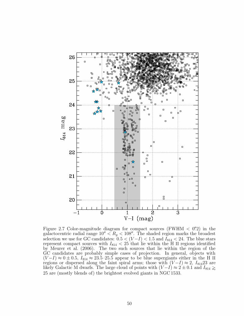
Figure 2.7 Color-magnitude diagram for compact sources (FWHM < 0.′′2) in thegalactocentric radial range 10′′ < Rg < 108′′. The shaded region marks the broadestselection we use for GC candidates: 0.5 < (V −I) < 1.5 and I814 < 24. The blue starsrepresent compact sources with I814 < 25 that lie within the H II regions identifiedby Meurer et al. (2006). The two such sources that lie within the region of theGC candidates are probably simple cases of projection. In general, objects with(V −I) ≈ 0 ± 0.5, I814 ≈ 23.5–25.5 appear to be blue supergiants either in the H IIregions or dispersed along the faint spiral arms; those with (V −I) ≈ 2, I81423 arelikely Galactic M dwarfs. The large cloud of points with (V −I) ≈ 2 ± 0.1 and I814 ∼>25 are (mostly blends of) the brightest evolved giants in NGC1533.
50
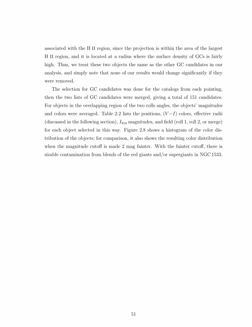
associated with the H II region, since the projection is within the area of the largest
H II region, and it is located at a radius where the surface density of GCs is fairly
high. Thus, we treat these two objects the same as the other GC candidates in our
analysis, and simply note that none of our results would change significantly if they
were removed.
The selection for GC candidates was done for the catalogs from each pointing,
then the two lists of GC candidates were merged, giving a total of 151 candidates.
For objects in the overlapping region of the two rolls angles, the objects’ magnitudes
and colors were averaged. Table 2.2 lists the positions, (V −I) colors, effective radii
(discussed in the following section), I814 magnitudes, and field (roll 1, roll 2, or merge)
for each object selected in this way. Figure 2.8 shows a histogram of the color dis-
tribution of the objects; for comparison, it also shows the resulting color distribution
when the magnitude cutoff is made 2 mag fainter. With the fainter cutoff, there is
sizable contamination from blends of the red giants and/or supergiants in NGC1533.
51

Table 2.2. GC Candidates
ID RA DEC (V −I)0 ± Reff I814 ± field
Number (J2000) (J2000) (mag) (mag) (arcsec) (mag) (mag)
13 62.478742 −56.109037 1.260 0.013 0.0207 22.759 0.024 merge
20 62.481901 −56.108821 1.341 0.024 0.0544 23.777 0.046 merge
30 62.494871 −56.107931 0.867 0.013 0.0307 22.467 0.014 merge
141 62.503620 −56.108303 1.082 0.014 0.0222 22.180 0.012 r2
175 62.469642 −56.111536 0.913 0.016 0.0340 22.856 0.034 merge
199 62.475854 −56.111165 0.863 0.011 0.0085 22.950 0.032 merge
219 62.456702 −56.113055 0.863 0.042 0.0159 23.580 0.058 merge
391 62.458113 −56.114010 0.855 0.011 0.0289 22.176 0.023 merge
424 62.477575 −56.112507 1.123 0.013 0.0377 22.120 0.019 merge
428 62.512621 −56.109436 1.299 0.017 0.0525 22.503 0.011 r2
443 62.468860 −56.113378 1.012 0.003 0.0237 21.869 0.022 merge
467 62.466586 −56.113788 1.086 0.011 0.0207 22.049 0.029 merge
472 62.470944 −56.113139 1.226 0.011 0.0277 21.610 0.018 merge
556 62.498873 −56.111763 0.816 0.011 0.0215 23.248 0.021 r2
566 62.486962 −56.112939 1.276 0.018 0.0592 23.898 0.054 r2
52

Table 2.2 (cont’d)
ID RA DEC (V −I)0 ± Reff I814 ± field
Number (J2000) (J2000) (mag) (mag) (arcsec) (mag) (mag)
616 62.507189 −56.111401 0.987 0.021 0.0629 23.863 0.026 r2
785 62.488994 −56.114282 0.806 0.065 0.0433 23.231 0.060 merge
883 62.473735 −56.116447 0.901 0.018 0.0163 22.738 0.034 merge
1030 62.487940 −56.116245 1.093 0.012 0.0296 20.884 0.011 merge
1048 62.491160 −56.116023 0.869 0.024 0.0355 23.966 0.052 merge
1151 62.483266 −56.117620 0.950 0.014 0.0300 19.897 0.011 merge
1238 62.494429 −56.117187 0.895 0.014 0.0696 23.727 0.039 r2
1336 62.474199 −56.119748 1.220 0.012 0.0266 20.723 0.013 merge
1388 62.475712 −56.120119 0.905 0.014 0.0244 20.775 0.013 merge
1398 62.487527 −56.119145 0.907 0.012 0.0455 22.925 0.028 merge
1542 62.472319 −56.121682 1.070 0.037 0.0355 23.399 0.065 merge
1550 62.469259 −56.122013 1.088 0.017 0.0141 22.218 0.036 r2
1607 62.483549 −56.121258 0.901 0.011 0.0289 21.363 0.013 merge
1633 62.490568 −56.120816 1.270 0.017 0.0037 23.301 0.033 r2
1645 62.468214 −56.122742 1.460 0.010 0.0141 22.868 0.053 r2
53
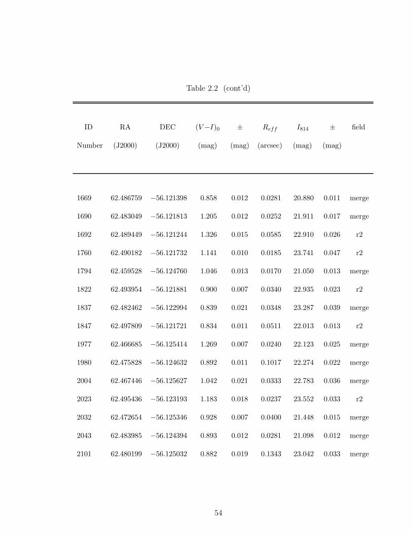
Table 2.2 (cont’d)
ID RA DEC (V −I)0 ± Reff I814 ± field
Number (J2000) (J2000) (mag) (mag) (arcsec) (mag) (mag)
1669 62.486759 −56.121398 0.858 0.012 0.0281 20.880 0.011 merge
1690 62.483049 −56.121813 1.205 0.012 0.0252 21.911 0.017 merge
1692 62.489449 −56.121244 1.326 0.015 0.0585 22.910 0.026 r2
1760 62.490182 −56.121732 1.141 0.010 0.0185 23.741 0.047 r2
1794 62.459528 −56.124760 1.046 0.013 0.0170 21.050 0.013 merge
1822 62.493954 −56.121881 0.900 0.007 0.0340 22.935 0.023 r2
1837 62.482462 −56.122994 0.839 0.021 0.0348 23.287 0.039 merge
1847 62.497809 −56.121721 0.834 0.011 0.0511 22.013 0.013 r2
1977 62.466685 −56.125414 1.269 0.007 0.0240 22.123 0.025 merge
1980 62.475828 −56.124632 0.892 0.011 0.1017 22.274 0.022 merge
2004 62.467446 −56.125627 1.042 0.021 0.0333 22.783 0.036 merge
2023 62.495436 −56.123193 1.183 0.018 0.0237 23.552 0.033 r2
2032 62.472654 −56.125346 0.928 0.007 0.0400 21.448 0.015 merge
2043 62.483985 −56.124394 0.893 0.012 0.0281 21.098 0.012 merge
2101 62.480199 −56.125032 0.882 0.019 0.1343 23.042 0.033 merge
54
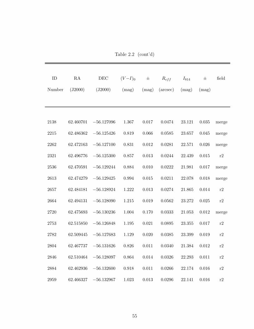
Table 2.2 (cont’d)
ID RA DEC (V −I)0 ± Reff I814 ± field
Number (J2000) (J2000) (mag) (mag) (arcsec) (mag) (mag)
2138 62.460701 −56.127096 1.367 0.017 0.0474 23.121 0.035 merge
2215 62.486362 −56.125426 0.819 0.066 0.0585 23.657 0.045 merge
2262 62.472163 −56.127100 0.831 0.012 0.0281 22.571 0.026 merge
2321 62.496776 −56.125300 0.857 0.013 0.0244 22.439 0.015 r2
2536 62.470591 −56.129244 0.884 0.010 0.0222 21.981 0.017 merge
2613 62.474279 −56.129425 0.994 0.015 0.0211 22.078 0.018 merge
2657 62.484181 −56.128924 1.222 0.013 0.0274 21.865 0.014 r2
2664 62.494131 −56.128090 1.215 0.019 0.0562 23.272 0.025 r2
2720 62.475693 −56.130236 1.004 0.170 0.0333 21.053 0.012 merge
2753 62.515850 −56.126848 1.195 0.021 0.0895 23.355 0.017 r2
2782 62.509445 −56.127683 1.129 0.020 0.0385 23.399 0.019 r2
2804 62.467737 −56.131626 0.826 0.011 0.0340 21.384 0.012 r2
2846 62.510464 −56.128097 0.864 0.014 0.0326 22.293 0.011 r2
2884 62.462936 −56.132600 0.918 0.011 0.0266 22.174 0.016 r2
2959 62.466327 −56.132967 1.023 0.013 0.0296 22.141 0.016 r2
55
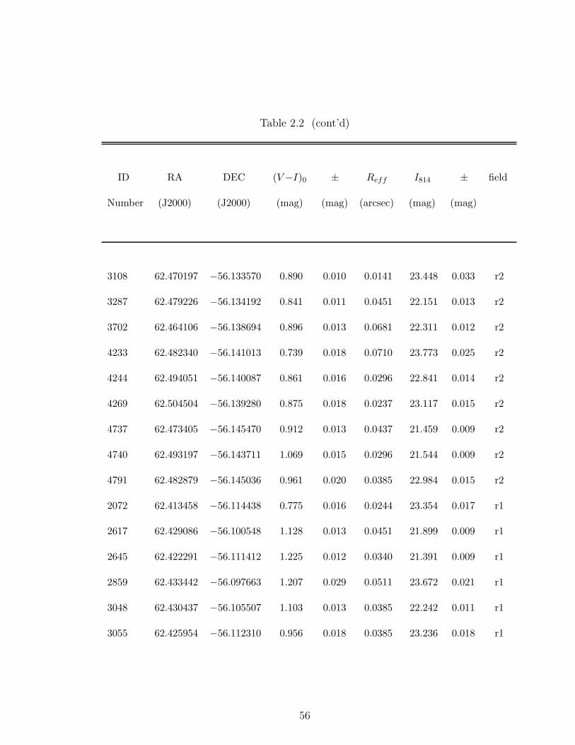
Table 2.2 (cont’d)
ID RA DEC (V −I)0 ± Reff I814 ± field
Number (J2000) (J2000) (mag) (mag) (arcsec) (mag) (mag)
3108 62.470197 −56.133570 0.890 0.010 0.0141 23.448 0.033 r2
3287 62.479226 −56.134192 0.841 0.011 0.0451 22.151 0.013 r2
3702 62.464106 −56.138694 0.896 0.013 0.0681 22.311 0.012 r2
4233 62.482340 −56.141013 0.739 0.018 0.0710 23.773 0.025 r2
4244 62.494051 −56.140087 0.861 0.016 0.0296 22.841 0.014 r2
4269 62.504504 −56.139280 0.875 0.018 0.0237 23.117 0.015 r2
4737 62.473405 −56.145470 0.912 0.013 0.0437 21.459 0.009 r2
4740 62.493197 −56.143711 1.069 0.015 0.0296 21.544 0.009 r2
4791 62.482879 −56.145036 0.961 0.020 0.0385 22.984 0.015 r2
2072 62.413458 −56.114438 0.775 0.016 0.0244 23.354 0.017 r1
2617 62.429086 −56.100548 1.128 0.013 0.0451 21.899 0.009 r1
2645 62.422291 −56.111412 1.225 0.012 0.0340 21.391 0.009 r1
2859 62.433442 −56.097663 1.207 0.029 0.0511 23.672 0.021 r1
3048 62.430437 −56.105507 1.103 0.013 0.0385 22.242 0.011 r1
3055 62.425954 −56.112310 0.956 0.018 0.0385 23.236 0.018 r1
56
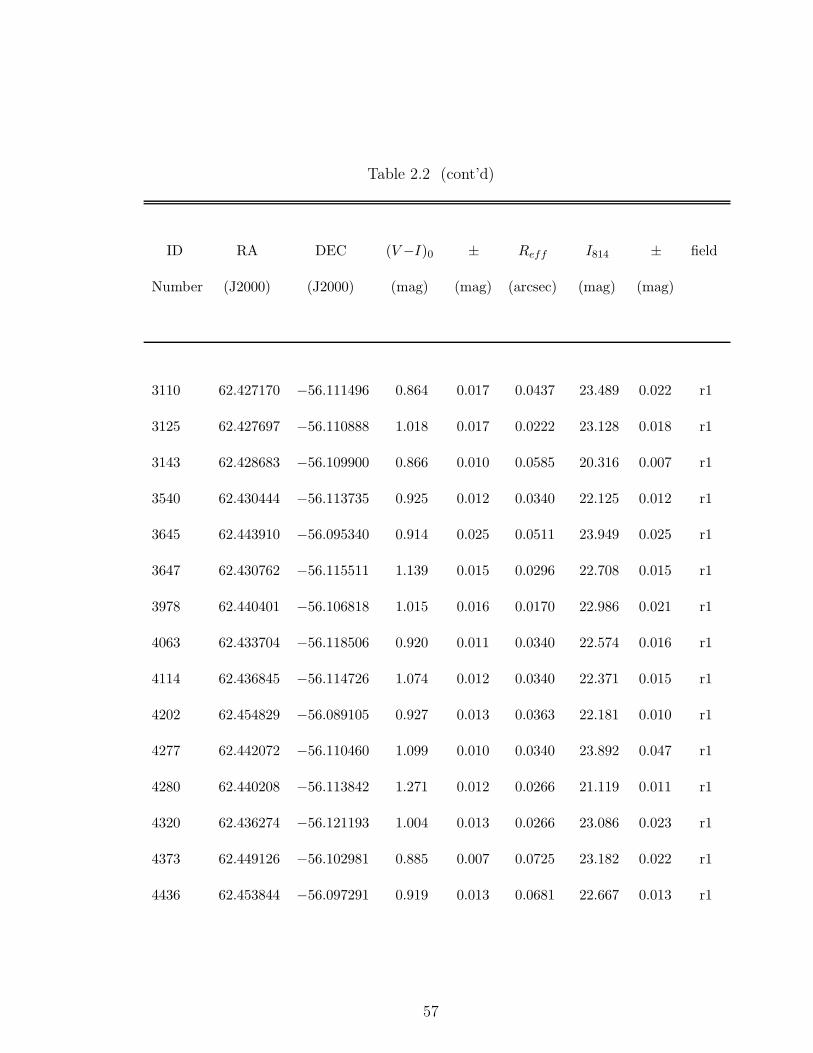
Table 2.2 (cont’d)
ID RA DEC (V −I)0 ± Reff I814 ± field
Number (J2000) (J2000) (mag) (mag) (arcsec) (mag) (mag)
3110 62.427170 −56.111496 0.864 0.017 0.0437 23.489 0.022 r1
3125 62.427697 −56.110888 1.018 0.017 0.0222 23.128 0.018 r1
3143 62.428683 −56.109900 0.866 0.010 0.0585 20.316 0.007 r1
3540 62.430444 −56.113735 0.925 0.012 0.0340 22.125 0.012 r1
3645 62.443910 −56.095340 0.914 0.025 0.0511 23.949 0.025 r1
3647 62.430762 −56.115511 1.139 0.015 0.0296 22.708 0.015 r1
3978 62.440401 −56.106818 1.015 0.016 0.0170 22.986 0.021 r1
4063 62.433704 −56.118506 0.920 0.011 0.0340 22.574 0.016 r1
4114 62.436845 −56.114726 1.074 0.012 0.0340 22.371 0.015 r1
4202 62.454829 −56.089105 0.927 0.013 0.0363 22.181 0.010 r1
4277 62.442072 −56.110460 1.099 0.010 0.0340 23.892 0.047 r1
4280 62.440208 −56.113842 1.271 0.012 0.0266 21.119 0.011 r1
4320 62.436274 −56.121193 1.004 0.013 0.0266 23.086 0.023 r1
4373 62.449126 −56.102981 0.885 0.007 0.0725 23.182 0.022 r1
4436 62.453844 −56.097291 0.919 0.013 0.0681 22.667 0.013 r1
57
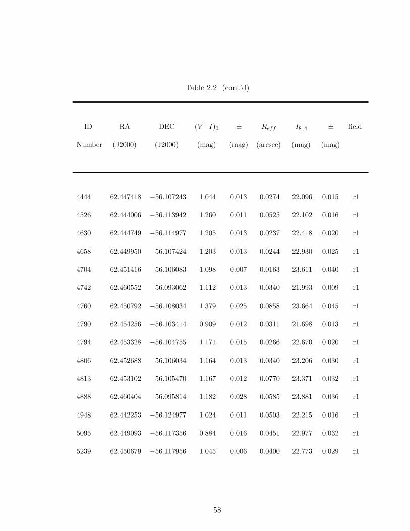
Table 2.2 (cont’d)
ID RA DEC (V −I)0 ± Reff I814 ± field
Number (J2000) (J2000) (mag) (mag) (arcsec) (mag) (mag)
4444 62.447418 −56.107243 1.044 0.013 0.0274 22.096 0.015 r1
4526 62.444006 −56.113942 1.260 0.011 0.0525 22.102 0.016 r1
4630 62.444749 −56.114977 1.205 0.013 0.0237 22.418 0.020 r1
4658 62.449950 −56.107424 1.203 0.013 0.0244 22.930 0.025 r1
4704 62.451416 −56.106083 1.098 0.007 0.0163 23.611 0.040 r1
4742 62.460552 −56.093062 1.112 0.013 0.0340 21.993 0.009 r1
4760 62.450792 −56.108034 1.379 0.025 0.0858 23.664 0.045 r1
4790 62.454256 −56.103414 0.909 0.012 0.0311 21.698 0.013 r1
4794 62.453328 −56.104755 1.171 0.015 0.0266 22.670 0.020 r1
4806 62.452688 −56.106034 1.164 0.013 0.0340 23.206 0.030 r1
4813 62.453102 −56.105470 1.167 0.012 0.0770 23.371 0.032 r1
4888 62.460404 −56.095814 1.182 0.028 0.0585 23.881 0.036 r1
4948 62.442253 −56.124977 1.024 0.011 0.0503 22.215 0.016 r1
5095 62.449093 −56.117356 0.884 0.016 0.0451 22.977 0.032 r1
5239 62.450679 −56.117956 1.045 0.006 0.0400 22.773 0.029 r1
58
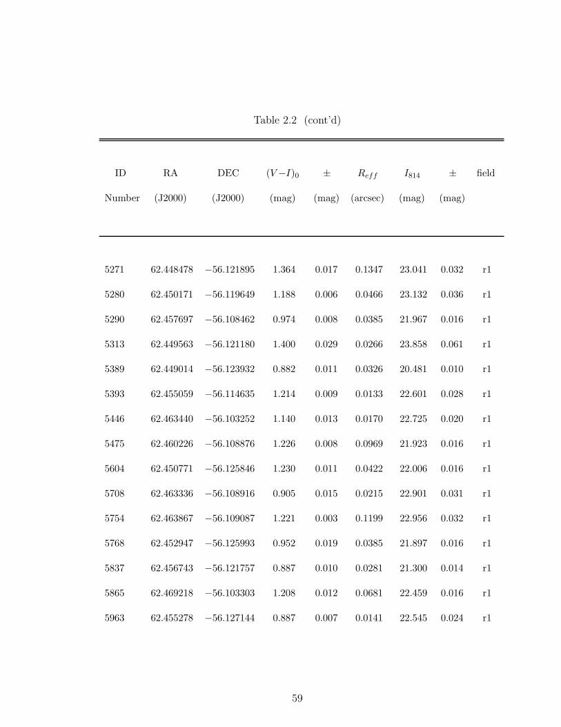
Table 2.2 (cont’d)
ID RA DEC (V −I)0 ± Reff I814 ± field
Number (J2000) (J2000) (mag) (mag) (arcsec) (mag) (mag)
5271 62.448478 −56.121895 1.364 0.017 0.1347 23.041 0.032 r1
5280 62.450171 −56.119649 1.188 0.006 0.0466 23.132 0.036 r1
5290 62.457697 −56.108462 0.974 0.008 0.0385 21.967 0.016 r1
5313 62.449563 −56.121180 1.400 0.029 0.0266 23.858 0.061 r1
5389 62.449014 −56.123932 0.882 0.011 0.0326 20.481 0.010 r1
5393 62.455059 −56.114635 1.214 0.009 0.0133 22.601 0.028 r1
5446 62.463440 −56.103252 1.140 0.013 0.0170 22.725 0.020 r1
5475 62.460226 −56.108876 1.226 0.008 0.0969 21.923 0.016 r1
5604 62.450771 −56.125846 1.230 0.011 0.0422 22.006 0.016 r1
5708 62.463336 −56.108916 0.905 0.015 0.0215 22.901 0.031 r1
5754 62.463867 −56.109087 1.221 0.003 0.1199 22.956 0.032 r1
5768 62.452947 −56.125993 0.952 0.019 0.0385 21.897 0.016 r1
5837 62.456743 −56.121757 0.887 0.010 0.0281 21.300 0.014 r1
5865 62.469218 −56.103303 1.208 0.012 0.0681 22.459 0.016 r1
5963 62.455278 −56.127144 0.887 0.007 0.0141 22.545 0.024 r1
59
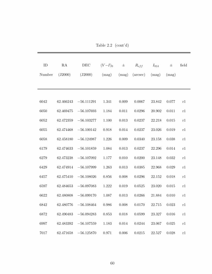
Table 2.2 (cont’d)
ID RA DEC (V −I)0 ± Reff I814 ± field
Number (J2000) (J2000) (mag) (mag) (arcsec) (mag) (mag)
6042 62.466243 −56.111291 1.341 0.009 0.0067 23.842 0.077 r1
6050 62.469475 −56.107693 1.184 0.011 0.0296 20.902 0.011 r1
6052 62.472359 −56.103277 1.100 0.013 0.0237 22.218 0.015 r1
6055 62.474468 −56.100142 0.918 0.014 0.0237 23.026 0.019 r1
6058 62.458180 −56.124987 1.226 0.009 0.0340 23.158 0.038 r1
6179 62.474633 −56.101859 1.084 0.013 0.0237 22.296 0.014 r1
6279 62.473238 −56.107092 1.177 0.010 0.0200 23.148 0.032 r1
6429 62.474914 −56.107999 1.263 0.013 0.0385 22.968 0.029 r1
6457 62.475410 −56.108026 0.856 0.008 0.0296 22.152 0.018 r1
6597 62.484653 −56.097083 1.222 0.019 0.0525 23.020 0.015 r1
6622 62.480808 −56.099170 1.087 0.013 0.0266 21.884 0.010 r1
6842 62.480776 −56.108464 0.986 0.008 0.0170 22.715 0.023 r1
6872 62.490483 −56.094283 0.853 0.018 0.0599 23.327 0.016 r1
6997 62.483392 −56.107559 1.183 0.014 0.0244 23.067 0.025 r1
7017 62.471658 −56.125870 0.971 0.006 0.0215 22.527 0.028 r1
60
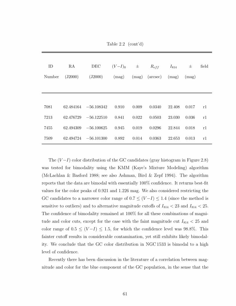
Table 2.2 (cont’d)
ID RA DEC (V −I)0 ± Reff I814 ± field
Number (J2000) (J2000) (mag) (mag) (arcsec) (mag) (mag)
7081 62.484164 −56.108342 0.910 0.009 0.0340 22.408 0.017 r1
7213 62.476729 −56.122510 0.841 0.022 0.0503 23.030 0.036 r1
7455 62.494309 −56.100625 0.945 0.019 0.0296 22.844 0.018 r1
7509 62.494724 −56.101300 0.892 0.014 0.0363 22.653 0.013 r1
The (V −I) color distribution of the GC candidates (gray histogram in Figure 2.8)
was tested for bimodality using the KMM (Kaye’s Mixture Modeling) algorithm
(McLachlan & Basford 1988; see also Ashman, Bird & Zepf 1994). The algorithm
reports that the data are bimodal with essentially 100% confidence. It returns best-fit
values for the color peaks of 0.921 and 1.226 mag. We also considered restricting the
GC candidates to a narrower color range of 0.7 ≤ (V −I) ≤ 1.4 (since the method is
sensitive to outliers) and to alternative magnitude cutoffs of I814 < 23 and I814 < 25.
The confidence of bimodality remained at 100% for all these combinations of magni-
tude and color cuts, except for the case with the faint magnitude cut I814 < 25 and
color range of 0.5 ≤ (V −I) ≤ 1.5, for which the confidence level was 98.8%. This
fainter cutoff results in considerable contamination, yet still exhibits likely bimodal-
ity. We conclude that the GC color distribution in NGC1533 is bimodal to a high
level of confidence.
Recently there has been discussion in the literature of a correlation between mag-
nitude and color for the blue component of the GC population, in the sense that the
61
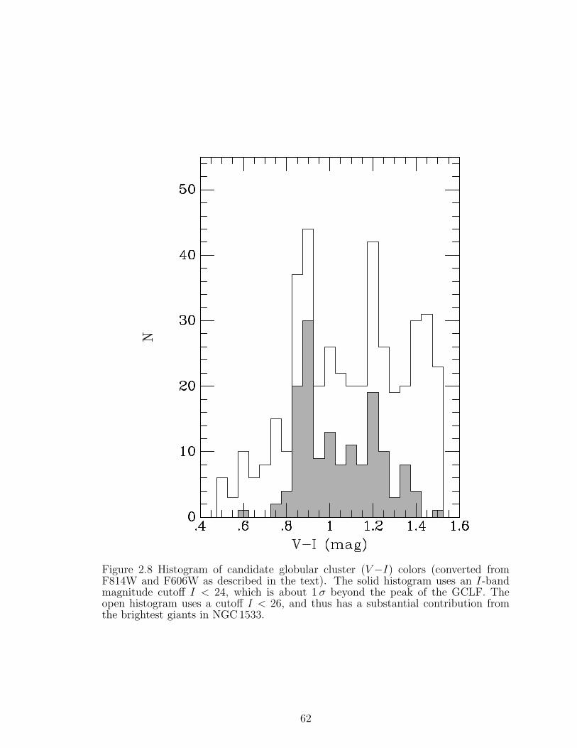
Figure 2.8 Histogram of candidate globular cluster (V −I) colors (converted fromF814W and F606W as described in the text). The solid histogram uses an I-bandmagnitude cutoff I < 24, which is about 1 σ beyond the peak of the GCLF. Theopen histogram uses a cutoff I < 26, and thus has a substantial contribution fromthe brightest giants in NGC1533.
62
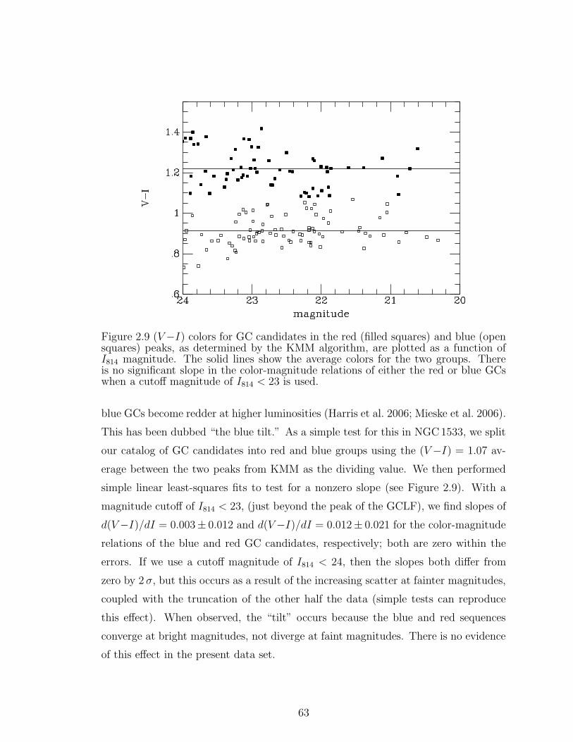
Figure 2.9 (V −I) colors for GC candidates in the red (filled squares) and blue (opensquares) peaks, as determined by the KMM algorithm, are plotted as a function ofI814 magnitude. The solid lines show the average colors for the two groups. Thereis no significant slope in the color-magnitude relations of either the red or blue GCswhen a cutoff magnitude of I814 < 23 is used.
blue GCs become redder at higher luminosities (Harris et al. 2006; Mieske et al. 2006).
This has been dubbed “the blue tilt.” As a simple test for this in NGC1533, we split
our catalog of GC candidates into red and blue groups using the (V −I) = 1.07 av-
erage between the two peaks from KMM as the dividing value. We then performed
simple linear least-squares fits to test for a nonzero slope (see Figure 2.9). With a
magnitude cutoff of I814 < 23, (just beyond the peak of the GCLF), we find slopes of
d(V −I)/dI = 0.003± 0.012 and d(V −I)/dI = 0.012± 0.021 for the color-magnitude
relations of the blue and red GC candidates, respectively; both are zero within the
errors. If we use a cutoff magnitude of I814 < 24, then the slopes both differ from
zero by 2 σ, but this occurs as a result of the increasing scatter at fainter magnitudes,
coupled with the truncation of the other half the data (simple tests can reproduce
this effect). When observed, the “tilt” occurs because the blue and red sequences
converge at bright magnitudes, not diverge at faint magnitudes. There is no evidence
of this effect in the present data set.
63
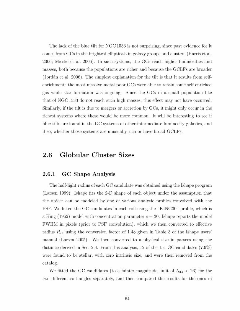
The lack of the blue tilt for NGC1533 is not surprising, since past evidence for it
comes from GCs in the brightest ellipticals in galaxy groups and clusters (Harris et al.
2006; Mieske et al. 2006). In such systems, the GCs reach higher luminosities and
masses, both because the populations are richer and because the GCLFs are broader
(Jordan et al. 2006). The simplest explanation for the tilt is that it results from self-
enrichment: the most massive metal-poor GCs were able to retain some self-enriched
gas while star formation was ongoing. Since the GCs in a small population like
that of NGC1533 do not reach such high masses, this effect may not have occurred.
Similarly, if the tilt is due to mergers or accretion by GCs, it might only occur in the
richest systems where these would be more common. It will be interesting to see if
blue tilts are found in the GC systems of other intermediate-luminosity galaxies, and
if so, whether those systems are unusually rich or have broad GCLFs.
2.6 Globular Cluster Sizes
2.6.1 GC Shape Analysis
The half-light radius of each GC candidate was obtained using the Ishape program
(Larsen 1999). Ishape fits the 2-D shape of each object under the assumption that
the object can be modeled by one of various analytic profiles convolved with the
PSF. We fitted the GC candidates in each roll using the “KING30” profile, which is
a King (1962) model with concentration parameter c = 30. Ishape reports the model
FWHM in pixels (prior to PSF convolution), which we then converted to effective
radius Reff using the conversion factor of 1.48 given in Table 3 of the Ishape users’
manual (Larsen 2005). We then converted to a physical size in parsecs using the
distance derived in Sec. 2.4. From this analysis, 12 of the 151 GC candidates (7.9%)
were found to be stellar, with zero intrinsic size, and were then removed from the
catalog.
We fitted the GC candidates (to a fainter magnitude limit of I814 < 26) for the
two different roll angles separately, and then compared the results for the ones in
64
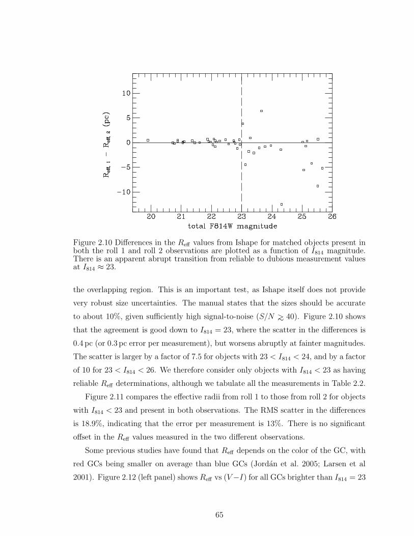
Figure 2.10 Differences in the Reff values from Ishape for matched objects present inboth the roll 1 and roll 2 observations are plotted as a function of I814 magnitude.There is an apparent abrupt transition from reliable to dubious measurement valuesat I814 ≈ 23.
the overlapping region. This is an important test, as Ishape itself does not provide
very robust size uncertainties. The manual states that the sizes should be accurate
to about 10%, given sufficiently high signal-to-noise (S/N ∼> 40). Figure 2.10 shows
that the agreement is good down to I814 = 23, where the scatter in the differences is
0.4 pc (or 0.3 pc error per measurement), but worsens abruptly at fainter magnitudes.
The scatter is larger by a factor of 7.5 for objects with 23 < I814 < 24, and by a factor
of 10 for 23 < I814 < 26. We therefore consider only objects with I814 < 23 as having
reliable Reff determinations, although we tabulate all the measurements in Table 2.2.
Figure 2.11 compares the effective radii from roll 1 to those from roll 2 for objects
with I814 < 23 and present in both observations. The RMS scatter in the differences
is 18.9%, indicating that the error per measurement is 13%. There is no significant
offset in the Reff values measured in the two different observations.
Some previous studies have found that Reff depends on the color of the GC, with
red GCs being smaller on average than blue GCs (Jordan et al. 2005; Larsen et al
2001). Figure 2.12 (left panel) shows Reff vs (V −I) for all GCs brighter than I814 = 23
65

Figure 2.11 Top: Measured Reff values for objects with I814 < 23 in roll 1 are plottedagainst the Reff values for the same objects measured in roll 2. The plotted line isequality. Bottom: Fractional differences in the Reff values are plotted as a functionof the average value. The solid line shows the mean offset of 0.038 ± 0.036.
66
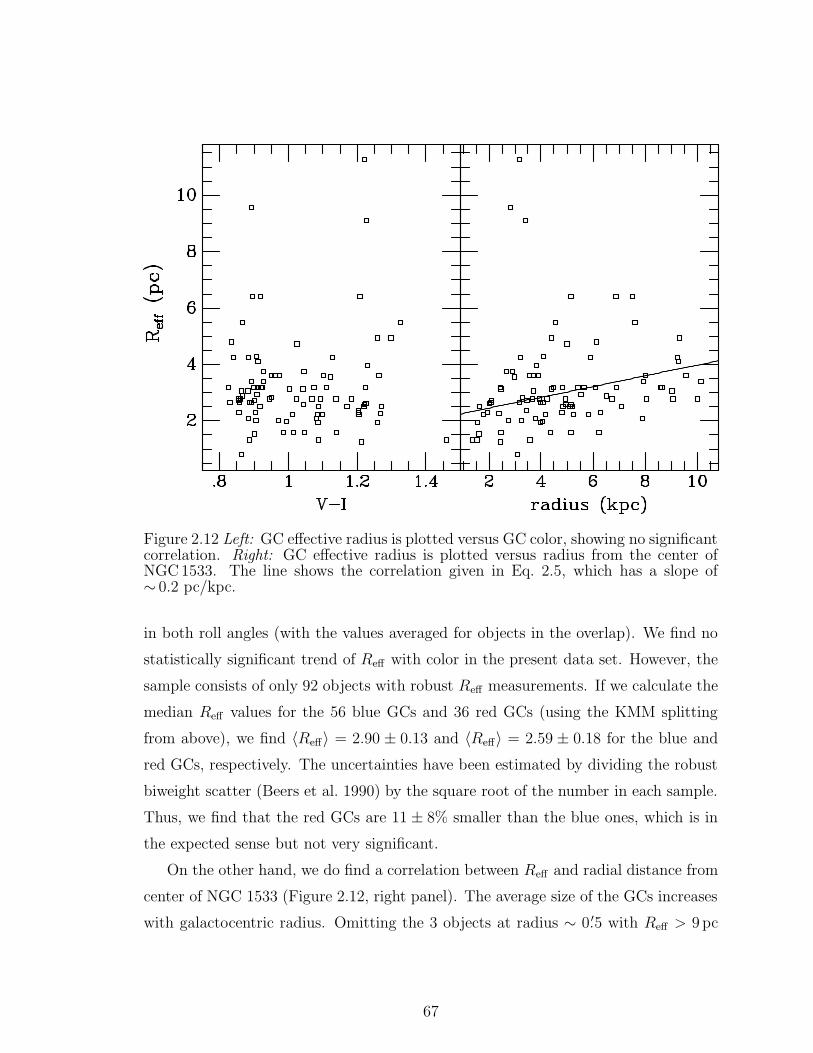
Figure 2.12 Left: GC effective radius is plotted versus GC color, showing no significantcorrelation. Right: GC effective radius is plotted versus radius from the center ofNGC1533. The line shows the correlation given in Eq. 2.5, which has a slope of∼ 0.2 pc/kpc.
in both roll angles (with the values averaged for objects in the overlap). We find no
statistically significant trend of Reff with color in the present data set. However, the
sample consists of only 92 objects with robust Reff measurements. If we calculate the
median Reff values for the 56 blue GCs and 36 red GCs (using the KMM splitting
from above), we find 〈Reff〉 = 2.90 ± 0.13 and 〈Reff〉 = 2.59 ± 0.18 for the blue and
red GCs, respectively. The uncertainties have been estimated by dividing the robust
biweight scatter (Beers et al. 1990) by the square root of the number in each sample.
Thus, we find that the red GCs are 11 ± 8% smaller than the blue ones, which is in
the expected sense but not very significant.
On the other hand, we do find a correlation between Reff and radial distance from
center of NGC 1533 (Figure 2.12, right panel). The average size of the GCs increases
with galactocentric radius. Omitting the 3 objects at radius ∼ 0.′5 with Reff > 9 pc
67

(which are more than 6 σ outliers), we find the following relation:
Reff = (2.83 ± 0.12) + (0.191 ± 0.047)[(Rg/1 kpc) − 4] pc, (2.5)
where Reff is in pc and galactocentric radius Rg is in kpc. Thus, we find a strong
correlation between Reff and radius Rg, significant at the 4 σ level, but no significant
correlation between Reff and color. NGC1533 is much more similar to the Milky
Way in this regard (e.g., van den Bergh et al. 1991) than to the early-type galaxies
in the Virgo cluster, where Reff has only a mild dependence on Rg but a significant
dependence on color (Jordan et al. 2005). It is tempting to associate this difference
with environment, but first it is necessary to study the behavior of Reff for the GCs
of many more galaxies in loose group environments.
2.6.2 Distance from Half-Light Radius
Using the extensive ACS Virgo Cluster Survey data set, Jordan et al. (2005)
have proposed a distance calibration based on the median half-light radius of the GC
population of a galaxy. From Eq. 19 of that paper, the distance d in Mpc to the
galaxy is estimated as
d =0.552 ± 0.058
〈rh〉Mpc, (2.6)
where 〈rh〉 is the corrected median half-light radius in arcseconds (their rh corresponds
to what we have called Reff , following the Ishape notation). Their definition of 〈rh〉involves small corrections based on galaxy z-band surface brightness, galaxy (g−z)
color, and GC (g−z) color. We do not have photometry in these bandpasses, and
although we might estimate conversions from models, Jordan et al. note that the
corrections are second-order; one can omit them for bright galaxies with broad GC
color distributions (as in NGC1533) and still obtain an accurate distance. Thus,
we simply take 〈rh〉 as equal to the median 〈Reff〉 = 0.′′0296 ± 0.′′0011 for the 92 GC
candidates in our catalog with I814 < 23. This gives a distance d = 18.6 ± 2.0 Mpc,
in accord with the distance of 19.4 ± 1.1 Mpc obtained from SBF in Sec. 2.4. The
agreement in distance implies that the sizes of the GCs in NGC1533 agree in the
68
median with those in the Virgo cluster and supports the use of GC half-light radii as
distance indicators.
2.7 Globular Cluster Luminosity Function
We used the maximum likelihood code from Secker (1992) to fit the globular cluster
luminosity function (GCLF) for 151 GC candidates down to a limit of I814 = 24. In
order to do this, it is necessary to have a reasonable estimate of the background
contamination. We searched the HST archive for possible background fields with
similar Galactic latitudes taken through the same F606W+F814W filter combination
to a similar depth. These fields were processed in the same way as the NGC1533 fields,
and the catalogs were subjected to the same selection according to their magnitude,
color, and FWHM. Some of these fields were found to be anomalously rich, as they
targeted distant rich clusters; these fields were excluded. In the end, we used four
background comparison fields.
For a Gaussian GCLF, we find a turnover (peak) I814 magnitude m0I = 22.84+0.18
−0.24
and dispersion σLF = 1.10 ± 0.15 mag. This GCLF is plotted in Figure 2.13. The
code also reports the confidence contours on the fit, as shown in Figure 2.14. We
performed various tests by changing the selection of the data, including narrowing
the color range to be between 0.7 and 1.4, varying the cutoff magnitude by ±0.5 mag,
and being more restrictive with the FWHM cut. These alternative selections changed
m0I by about ±0.1 mag, and σLF by about ±0.05 mag, both well within the quoted
errors.
Our SBF distance together with the measured m0I implies M0
I = −8.6+0.22−0.27 for
NGC1533. Conversely, the GCLF measurement provides another estimate of the
distance, if we have a calibration for M 0I . Harris (2001) gives a V -band calibration
〈M0V 〉 = −7.4±0.2, where we use the quoted scatter as an estimate of the uncertainty.
This zero point assumes a Virgo distance modulus of 30.97, which is 0.12 mag less
than the calibration used for the ACS Virgo Cluster Survey and in this work. If
we adjust for this offset and assume 〈V −I〉 = 1.07 mag (Sec. 2.5; Kissler-Patig &
69

Figure 2.13 The GCLF of candidate globular clusters. The thick solid curve is amaximum likelihood fit to the (unbinned) GC magnitude distribution, representedby the histogram. The dashed line shows the limiting magnitude used for the fit.
70
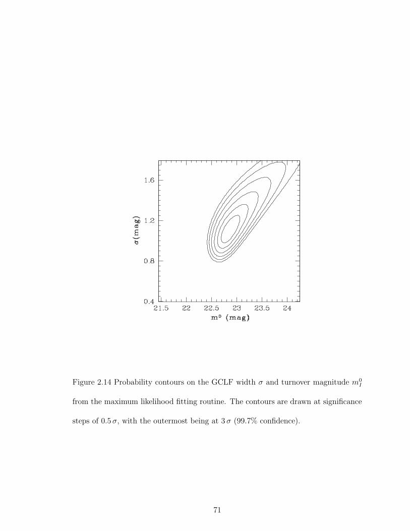
Figure 2.14 Probability contours on the GCLF width σ and turnover magnitude m0I
from the maximum likelihood fitting routine. The contours are drawn at significance
steps of 0.5σ, with the outermost being at 3 σ (99.7% confidence).
71

Gebhardt 1999), then we have 〈M 0I 〉 = −8.59, giving (m−M) = 31.41 ± 0.29 mag.
This is consistent with the measured SBF distance and the distance estimated from
the GC half-light radii. Note, however, that if we had used the value of 〈M 0V 〉 given
by Harris for S0 galaxies, or if we had converted from the value of 〈M 0z 〉 given by
Jordan et al. (2006), then the inferred distance modulus would have been larger by
about 0.2 mag, although still in agreement within the errors.
Jordan et al. (2006) have found a correlation for Virgo galaxies of the GCLF
width with galaxy B luminosity, and we can test whether or not NGC1533 follows
this trend. The total apparent B-band magnitude of NGC1533 from the RC3 is 11.7.
With our measured (m−M), Eq. (2) from Jordan et al. (2006) predicts σLF = 1.09
mag, in excellent agreement with our measured value of 1.10±0.15 mag. We conclude
that the GCLF of NGC1533 is consistent within the uncertainties with those observed
in Virgo.
Finally, we can estimate the value of the GC specific frequency SN = NGC ×100.4(MV +15) (Harris & van den Bergh 1981), where NGC is the number of globulars
and MV is the absolute magnitude of the galaxy. The GCLF analysis indicates that
the number of GCs integrated over luminosity is 163 ± 20 in the region analyzed.
We used an outer radial limit of 1.′8 for this study, but a significant portion of the
area within this radius is missing as a result of the proximity of the galaxy to the
image edge at both roll angles and the necessity of omitting the inner 10′′. If we make
the reasonable assumption that the “missing” GCs roughly follow the galaxy light
within 1.′8, then we find a total population NGC = 250 ± 30 within this radius. The
total V magnitude of the galaxy within the same radius is V = 10.75, and using the
measured distance modulus, we find SN = 1.3 ± 0.2. We expect this is very close to
the “global” value, as < 5% of the light (based on the galaxy profile modeling), and
few candidate GCs, are beyond this radius (which motivated the choice of radius).
This result for NGC1533 agrees well with the mean local SN = 1.0± 0.6 reported by
Kundu & Whitmore (2001) from HST/WFPC2 imaging of nearby S0 galaxies.
72
2.8 Conclusions
We have analyzed deep F606W and F814W images of the galaxy NGC1533 and
its GC population taken at two roll angles with the ACS/WFC on HST. Although it
is classified as an early-type barred lenticular galaxy, we found faint spiral structure
once a smooth fit to the galaxy isophotes was subtracted. The color map shows faint
dust features in the area around the bar and inner disk. Previous ground-based Hα
imaging had shown that the galaxy disk contains several (∼ 5) faint, compact H II
regions. We find that all of these regions have luminous blue stars within them,
although in some cases only one such star is evident. Four of these H II regions lie
within one of the faint spiral arms, and a few other blue stars spread out within the
arm. These observations suggest that NGC1533 is in the late stages of a transition
in morphology from type SBa to SB0.
From two-dimensional two-component parametric modeling of the galaxy surface
brightness, we find a bulge-to-total ratio B/T ≈ 0.42. The half-light radii of the
bulge and disk are ∼ 7′′ and ∼ 46′′, respectively. We find a best-fitting Sersic index
n = 2.0 for the bulge, which can be reasonably approximated by an r1/4 law in the
1-D profile. However, the disk has a relatively flat profile over a factor-of-three in
radius, from ∼ 15′′ to ∼ 45′′, then steepens fairly abruptly beyond ∼ 50′′. This gives
the disk a very low Sersic index of n ≈ 0.4, which might result from past high-speed
interactions of NGC1533 within the group environment.
Overall, the color of NGC1533 is that of an evolved, red population, except in the
few, small isolated regions where the blue stars occur. The bulge color is (V −I) >
1.22, similar to cluster ellipticals, and then there is a mild, but significant, linear color
gradient throughout the disk. There is a gradual isophotal twist, and the isophotes
increase in ellipticity from the bulge to a semi-major axis distance of 24′′, where ε goes
above 0.4 before falling sharply again towards the round outer disk. The peak of the
A4 harmonic term, measuring “diskiness,” actually occurs at a smaller semi-major
axis of 21′′. This is because the pointed lens-like isophotes occur inside of the bar.
We measured the SBF amplitude in four broad radial annuli for each of the two ob-
servations at different roll angles. A gradient in the SBF amplitude is clearly detected
73
and follows the color gradient (the bluer outer regions have relatively brighter SBF).
By matching our ACS photometry against ground-based (V −I) data for this galaxy,
we have accurately calibrated the SBF measurements to obtain distance moduli. We
find excellent agreement among the different annuli but with an offset of 0.04 mag
in distance between the two observations. However, the distance error is dominated
by systematic uncertainty in the color and calibration zero point. We find a final
distance modulus (m−M) = 31.44 ± 0.12 mag, or d = 19.4 ± 1.1 Mpc.
Candidate globular clusters were selected according to color, magnitude, radial
position, and FWHM. Analysis of the color distribution of these objects with the
KMM algorithm indicates with a very high degree of confidence that the distribution is
bimodal. There is no evidence that the blue GCs become redder at bright magnitudes,
the so-called “blue tilt.” The absence of this effect in NGC1533, an intermediate
luminosity galaxy with a small GC population, is consistent with a self-enrichment
explanation, since the GCs in such systems do not reach the high masses that they
do in richer systems. The sizes of the GC candidates were measured using the Ishape
software. By comparing the results from the two different roll angles, we found that
the effective (half-light) radii Reff have an accuracy of about 13% down to I814 = 23,
but are not reliable beyond this. We did not find a significant trend of Reff with GC
color, although the red-peak GCs have a median Reff smaller by 11 ± 8% than the
blue-peak GCs.
However, we did find a significant (4σ) trend of Reff with galactocentric radius.
In this respect, NGC1533 is more like the Milky Way than the Virgo early-type
galaxies. This may be an effect of the environment: since the sizes of the GCs are
limited by the tidal field, and the density gradients will be steeper in small groups
such as Dorado or the Local Group, GC sizes should have a stronger dependence
on radius in such environments. The dominance of this radial effect may weaken or
obscure any relation between size and color. More studies of size and color trends for
the GCs of galaxies in loose groups are needed to verify this hypothesis, although this
may be difficult because of the low GC populations in such systems. We then used the
median half-light GC radius to obtain another estimate of the distance to NGC1533.
Following Jordan et al. (2005), we find d = 18.6 ± 2.0 Mpc, in good agreement with
74

the SBF distance.
We modeled the I814-band GCLF of NGC1533 as a Gaussian using a maximum
likelihood fitting routine. The best-fit peak magnitude m0I = 22.84+0.18
−0.24 corresponds
to M0I ≈ −8.6 for the measured SBF distance, in good agreement with expectations
based on other galaxies. The fitted Gaussian dispersion of σLF = 1.10 ± 0.15 mag
is in accord with the relation between σLF and galaxy luminosity found recently by
Jordan et al. (2006) for Virgo galaxies. Finally we estimate the GC specific frequency
in the analysis region to be SN = 1.3 ± 0.2, typical for a disk galaxy. We conclude
that the GCs in NGC1533 have the same average size, color, and luminosity within
the errors as the Virgo early-type galaxies, but the stronger dependence of size on
galactocentric distance is more reminiscent of the Milky Way.
NGC1533 represents an interesting class of transitional objects, both in terms of
morphology and environment. A large, multi-band, systematic study of such systems
with HST, similar to the ACS Virgo and Fornax Cluster surveys but focusing on
group galaxies, has yet to be undertaken and must await either a revived ACS or
Wide Field Camera 3. Such an effort would be extremely valuable in piecing together
a more complete picture of the interplay between galaxy structure, globular cluster
system properties, and environment.
75
Bibliography
[1] Ajhar, E. A., Lauer, T. R., Tonry, J. L., Blakeslee, J. P., Dressler, A., Holtzman,
J. A., & Postman, M. 1997, AJ, 114, 626
[1] Ashman, K. M., Bird, C. M., & Zepf, S. E. 1994, AJ, 108, 2348
[1] Ashman, K. M., & Zepf, S. E. 1998, Globular Cluster Systems (New York: Cam-
bridge University Press)
[4] Beers, T. C., Flynn, K., & Gebhardt, K. 1990, AJ, 100, 32
[8] Benıtez, N., et al. 2004, ApJS, 150, 1
[6] Bernardi, M., Alonso, M.V., da Costa L.N., Willmer, C.N.A., Wegner, G., Pelle-
grini, P.S., Rite, and Maia, M.A.G. 2002, AJ, 123, 2990
[4] Bertin, E., & Arnouts, S. 1996, A&AS, 117, 393
[8] Blakeslee, J. P., Ajhar, E. A., & Tonry, J. L. 1999, Post-Hipparcos Cosmic Can-
dles, 237, 181
[4] Blakeslee, J. P., Anderson, K. R., Meurer, G. R., Benıtez, N., & Magee, D. 2003,
Astronomical Data Analysis Software and Systems XII, 295, 257
[10] Blakeslee, J. P., Lucey, J. R., Tonry, J. L., Hudson, M. J., Narayanan, V. K., &
Barris, B. J. 2002, MNRAS, 330, 443
[11] Blakeslee, J. P., Vazdekis, A., & Ajhar, E. A. 2001, MNRAS, 320, 193
76
[12] Brown, T. M., et al. 2005, AJ, 130, 1693
[13] Buta, R., Corwin, H., & Odewahn, S. 2006, The De Vaucouleurs Atlas of Galaxies
(Cambridge: Cambridge Univ. Press)
[14] Cantiello, M., Blakeslee, J. P., Raimondo, G., Mei, S., Brocato, E., & Capaccioli,
M. 2005, ApJ, 634, 239
[15] Cantiello, M., Raimondo, G., Brocato, E., & Capaccioli, M. 2003, AJ, 125, 2783
[16] Cantiello, M., Raimondo, G., Blakeslee, J. P., Brocato, E., & Capaccioli, M.
2007, ApJ, 662, 940
[17] Cote, P., Blakeslee, J.P., Ferrarese, L., Jordan, A., Mei, S., Merritt, D., Milosavl-
jevic, M., Peng, E.W., Tonry., J.L., & West, M.J. 2004, ApJS, 153, 223
[de Vaucouleurs et al. 1991] de Vaucouleurs, G., de Vaucouleurs, A., Corwin, H. G.,
Jr., Buta, R. J., Paturel, G., & Fouque, P. 1991, Third Reference Catalog of Bright
Galaxies (New York: Springer-Verlag) (RC3)
[18] Ferguson, H.C., & Sandage, A. 1990, AJ, 100, 1
[19] Ferrarese, L., et al. 2006, ApJS, 164, 334
[20] Firth, P., Evstigneeva, E.A., Jones, J.B., Drinkwater, M.J., Phillips, S., & Gregg,
M.D. 2006, MNRAS, 372, 1856
[21] Freedman, W. L., et al. 2001, ApJ, 553, 47
[Gebhardt & Kissler-Patig 1999] Gebhardt, K. & Kissler-Patig, 1999, AJ, 118, 1526
[22] Harris, W. E. 2001, Saas-Fee Advanced Course 28: Star Clusters, 223
[10] Harris, W. E., & van den Bergh, S. 1981, AJ, 86, 1627
[12] Harris, W. E., Whitmore, B. C., Karakla, D., Okon, W., Baum, W. A., Hanes,
D. A., & Kavelaars, J. J. 2006, ApJ, 636, 90
77

[25] Jedrzejewski, R. I. 1987, MNRAS, 226, 747
[26] Jensen, J. B., Tonry, J. L., & Luppino, G. A. 1998, ApJ, 505, 111
[27] Jones, D.H., Saunders, W., Read, M., & Colless, M. 2005, PASA, 22, 277
[27] Jordan, A., et al. 2004, ApJS, 154, 509
[29] Jordan, A., et al. 2005, ApJ, 634, 1002
[30] Jordan, A., et al. 2006, ApJ, 651, L25
[31] Jordan, A., Blakeslee, J.P., Cote, P., Ferrarese, L., Infante, L., Mei, S., Merritt,
D., Peng, E.W., Tonry., J.L., & West, M.J. 2007, ApJS, 169, 213
[32] Jorgensen, I. 1997, MNRAS, 288, 161
[33] Kilborn, V. A., Koribalski, B. S., Forbes, D. A., Barnes, D. G., & Musgrave,
R. C. 2005, MNRAS, 356, 77
[34] Kissler-Patig, M., & Gebhardt, K. 1999, Astronomische Gesellschaft Meeting
Abstracts, 15, 1
[35] Kundu, A., & Whitmore, B. C. 2001, AJ, 122, 1251
[14] King, I. 1962, AJ, 67, 471
[krist2003] Krist, J. 2003, ISR ACS-2003-06 (Baltimore: STScI)
[30] Larsen, S. S. 1999, A&AS, 139, 393
[Larsen & Richtler 2000] Larsen, S.S., & Richtler, T. 2000, A&A, 354, 836
[38] Larsen, S. S., Forbes, D. A., & Brodie, J. P. 2001, MNRAS, 327, 1116
[39] Laurikainen, E., Salo, H., Buta, R., Knapen, J., Speltincx, T., & Block, D. 2006,
AJ, 132, 2634
[40] Liu, M. C., Charlot, S., & Graham, J. R. 2000, ApJ, 543, 644
78

[41] Mei, S., et al. 2005, ApJS, 156, 113
[42] McLachlan, G. J., & Basford, K. E. 1988, Mixture models. Inference and appli-
cations to clustering (Statistics: Textbooks and Monographs, New York: Dekker,
1988)
[43] Maoz, D., Barth, A.J., Sternberg, A., Filippenko, A.V., Ho, L.C., Macchetto,
F.D., Rix, H.-W., & Schneider, D.P. 1996, AJ, 111, 2248
[44] Meurer, G.R., Heckman, T.M., Leitherer, C., Kinney, A., Robert, C., & Garnett,
D.R. 1995 AJ, 110, 2665
[45] Meurer, G. R., et al. 2006, ApJS, 165, 307
[14] Mieske, S., et al. 2006, ApJ, 653, 193
[37] Peng, C. Y., Ho, L. C., Impey, C. D., & Rix, H. 2002, AJ, 124, 266
[9] Peng, E. W., et al. 2006, ApJ, 639, 95
[10] Ryan-Weber, E. V., et al. 2004, AJ, 127, 1431
[50] Sandage, A., & Brucato, R. 1979, AJ, 84, 472
[13] Schlegel, D. J., Finkbeiner, D. P., & Davis, M. 1998, ApJ, 500, 525
[52] Secker, J. 1992, AJ, 104, 1472
[40] Sersic, J. L. 1968, Cordoba, Argentina: Observatorio Astronomico, 1968
[41] Sirianni, M., et al. 2005, PASP, 117, 1049
[45] Tonry, J. L., Blakeslee, J. P., Ajhar, E. A., & Dressler, A. 1997, ApJ, 475, 399
[56] Tonry, J. L., Dressler, A., Blakeslee, J. P., Ajhar, E. A., Fletcher, A. B., Luppino,
G. A., Metzger, M. R., & Moore, C. B. 2001, ApJ, 546, 681
[57] van den Bergh, S., Morbey, C., & Pazder, J. 1991, ApJ, 375, 594
79

[58] West, M. J., Cote, P., Marzke, R. O., & Jordan, A. 2004, Nature, 427, 31
[59] Whitmore, B.C., & Schweizer, F. 1995, AJ, 109, 960
[60] Whitmore, B.C., Zhang, Q., Leitherer, C., Fall, S.M., Schweizer, F., & Miller,
B.W. 1999, AJ, 118, 1551
80
Chapter 3
Ultra-Compact Dwarf Candidates
Near the Lensing Galaxy in Abell
S0740
This chapter was published under the same title in The Astrophysical Journal,
Vol136, Issue 6, pp 2295-2305, (2008). The work presented in Chapter 3 was under-
taken in collaboration with Dr. John Blakeslee.
Synopsis
We analyze three-band imaging data of the giant elliptical galaxy ESO325-G004
from the Hubble Space Telescope Advanced Camera for Surveys (ACS). This is the
nearest known strongly lensing galaxy, and it resides in the center of the poor cluster
Abell S0740 at redshift z = 0.034. Based on magnitude, color, and size selection
criteria, we identify a sample of 15 ultra-compact dwarf (UCD) galaxy candidates
81

within the ACS field. This is comparable to the numbers of UCDs found within
similar regions in more nearby clusters (Virgo, Fornax, Hydra). We estimate circular
half-light radii Re,c from 2-D Sersic and King model fits and apply an upper cutoff
of 100 pc for our UCD selection. The selected galaxies have typical Sersic indices
n≈ 1.5, while larger sources with Re,c > 100 pc are more nearly exponential, perhaps
indicating that the latter are dominated by background disk galaxies. Many of the
UCD candidates are surrounded by a faint “fuzz” of halo light, which may be the
remnants of stripped material, and there is some evidence for intrinsic flattening of
the UCDs themselves. An apparent separation in size between the most compact
UCDs with Re,c < 17 pc and larger ones with Re,c > 40 pc may hint at different
formation mechanisms. We do not find any M32 analogues in this field. The colors
of the UCD candidates span the range from blue to red globular clusters, although
the brightest ones are predominantly red. The UCD candidates follow the flattened,
elliptical distribution of the globular clusters, which in turn follow the galaxy halo
light, suggesting a common evolution for these three components. Planned follow-up
spectroscopy can determine which candidates are truly members of Abell S0740 and
how similar they are in distribution to the globulars.
3.1 Introduction
A new class of stellar system has emerged in recent years. Due to the size of these
objects, being larger than average globular clusters (GCs) and smaller than dwarf
galaxies, they have been dubbed ultra-compact dwarf galaxies, or UCDs (Phillips
et al. 2001). They are typically a few ×107 M� in mass, with effective radii in
the range 10-100 pc. First discovered in the Fornax Cluster (Hilker et al. 1999;
Drinkwater et al. 2000), UCDs have now been found in significant numbers in the
Virgo, Centaurus, and Hydra clusters (Hasegan et al. 2005; Mieske et al 2007; Wehner
& Harris 2007), all systems within ∼ 50 Mpc of the Local Group. They are apparently
very rare outside of galaxy clusters (Evstigneeva et al. 2007b).
As they have absorption line spectra and appear to be transitional between GCs
82

and early-type dwarfs (cf. Hasegan et al. 2005), there are two basic ideas for the nature
of UCDs: they are related to globulars, or to dwarf galaxies. More specifically, UCDs
may be the largest members of the rich GC populations found inside galaxy clusters
(Mieske et al. 2002), possibly growing to such large size through dissipational merging
early in their lifetimes (Fellhauer & Kroupa 2002). Or, they may be the small, tidally
stripped remains of nucleated dwarf galaxies on orbits that carried them too close to
the center of the cluster potential (Bekki et al. 2001; Drinkwater et al. 2003). This
latter explanation has come to be known as galaxy “threshing,” but the idea has been
around for many years. Bassino et al. (1994) numerically simulated the evolution of
nucleated dwarfs in Virgo and showed that stripped nuclei could constitute a large
fraction of M87’s very rich GC system, while larger UCD-like remnants would occur
farther out. Recent Hubble Space Telescope (HST) imaging has revealed nuclei in
a much higher percentage of Virgo early-type dwarfs than previously thought (Cote
et al. 2006). Thus, stripping of nucleated dwarfs may account for both UCDs and
many of the GCs in the center of cluster potentials.
Some evidence based on the color-magnitude sequence of UCDs suggests that they
may be an extension of the red GC component to brighter magnitudes (Wehner &
Harris 2007). The UCDs in the Virgo and Fornax clusters also have spectroscopic
metallicities and α-element enhancements consistent with their being the high-mass
mass extreme of the red GC population (Evstigneeva et al. 2007a; Mieske et al.
2006), and less consistent with simple versions of the threshing model. Estigneeva
et al. (2008) attempted to distinguish between the two formation scenarios on the
basis of the structural properties of UCDs in the nearby Virgo and Fornax clusters
measured using the HST High Resolution Channel. Even with such high resolution
measurements, the data were consistent with either explanation, although more de-
tailed predictions of the size evolution of the nuclei during threshing are needed to test
this scenario. The relatively low velocity dispersions of cluster UCD populations are
expected in either model (e.g., Bekki 2007). However, detailed comparison between
the spatial distributions of large samples of UCDs and their possible nucleated dwarf
progenitors in clusters may help uncover their evolutionary histories (e.g., Goerdt
et al. 2008; Thomas et al. 2008).
83
Given the difficulty in distinguishing between the formation scenarios, further
UCD surveys can provide valuable information on the properties of this new type
of stellar system. A larger sample of groups and clusters is especially useful for
constraining environmental effects on the formation of UCDs. Here, we present a
search with HST for UCD candidates near ESO325-G004, the central giant elliptical
in Abell S0740. This is one of the systems in the supplementary list of poor clusters
tabulated by Abell et al. (1989) that did not meet the lowest richness criteria of the
original Abell (1958) catalogue. The cluster velocity dispersion is only ∼ 300 km s−1
(see plot in Smith et al. 2005), similar to that of Fornax, where UCDs were first
discovered. The absolute V magnitude of ESO325-G004 is MV = −23.2, making
it about 60% more luminous than M87, or 2.5 times the luminosity of NGC1399 in
Fornax. At z = 0.034, ESO325-G004 is also the closest known gravitational lens and
has both dynamical and lensing mass estimates (Smith et al. 2005). This makes it
an interesting target for UCD searches, since it is a very massive, dominant elliptical
in a poor cluster or rich group environment.
The following section describes our data in detail. In § 3.3, we present our pho-
tometric and size measurements and discuss the selection of UCD candidates. The
properties of the UCD candidates are discussed in § 3.4 and compared with those
of GCs and other objects in the field. The final section summarizes the results.
Throughout this paper, we use the WMAP 3-year cosmology results (Spergel et al.
2007) and assume a distance modulus for ESO325-G004 of (m−M) = 35.78 mag, or
a luminosity distance of 143 Mpc, and an angular scale of 0.65 kpc arcsec−1. This
translates to an image scale of about 33 pc pix−1 for our observations with Advanced
Camera for Surveys Wide Field Channel (ACS/WFC).
3.2 Observations and Reductions
ESO325-G004 was imaged with the ACS/WFC in the F475W, F625W, and F814W
filters. Throughout this paper, we refer to magnitudes in these filters as g475, r625, and
I814, respectively. The galaxy was initially observed in F814W and F475W as part of
84
HST GO Program 10429 during January 2005. This program, which is conducting a
surface brightness fluctuation survey in the Shapley supercluster region, is described
in Blakeslee (2007). There were 22 F814W exposures of varying times totaling of
18,882 s, and three exposures in F475W of 367s each. In February 2006, further
imaging of the ESO325-G004 field was carried out by HST DD Program 10710 for
a Hubble Heritage public release image.1 This provided six additional exposures in
each of the F475W and F625W filters. The total exposure times for this field were
therefore 5901, 4650, and 18882 s in F475W, F625W, and F814W, respectively.
The images were processed with the Apsis pipeline (Blakeslee et al. 2003) to pro-
duce summed, geometrically corrected, cosmic ray cleaned images for each bandpass.
Figure 3.1 shows a color composite image constructed from the data in the three
bandpasses. Apsis corrects the astrometric zero point of the images to within an
uncertainty of about 0.′′1. It also produces an RMS image giving the total noise
for each pixel. We calibrated the photometry using the Vega-based ACS/WFC zero
points for each filter from Sirianni et al. (2005): mg475 = 26.168, mr625 = 25.731,
and mI814 = 25.501. We corrected the photometry for Galactic extinction using
E(B−V ) = 0.0605 mag (Schlegel et al. 1998) and the extinction ratios from Sirianni
et al. (2005). We find the following extinction corrections in each band: A475 = 0.217
mag, and A625 = 0.159 mag, and A814 = 0.109 mag.
We modeled the main galaxy ESO325-G004 using the elliprof software (Tonry
et al. 1997), as well as several of the other smaller galaxies in the field to obtain a
better fit. The small galaxy models were subtracted from the image, and bright stars,
diffraction spikes, and other galaxies were masked so a final model of ESO325-G004
could be made. This final model was then subtracted to create a residual image,
which was used to find sources with the object detection software SExtractor (Bertin
& Arnouts 1996). We used the Apsis RMS image, which includes the noise from
the subtracted galaxies, for the SExtractor detection weighting. To the F814W RMS
image, we also added additional noise to account for the galaxy surface brightness
fluctuations, as described in more detail by Jordan et al. (2004) and Barber DeGraaff
1http://heritage.stsci.edu/2007/08/index.html
85

E
N
Figure 3.1 Hubble Space Telescope ACS/WFC image of ESO325-G004, showing about3.′0× 3.′3 of the field at the observed orientation. This color composite was constructedby the Hubble Heritage Team (STScI/AURA) from our imaging in the F475W (g),F625W (r), and F814W (I) bandpasses.
86
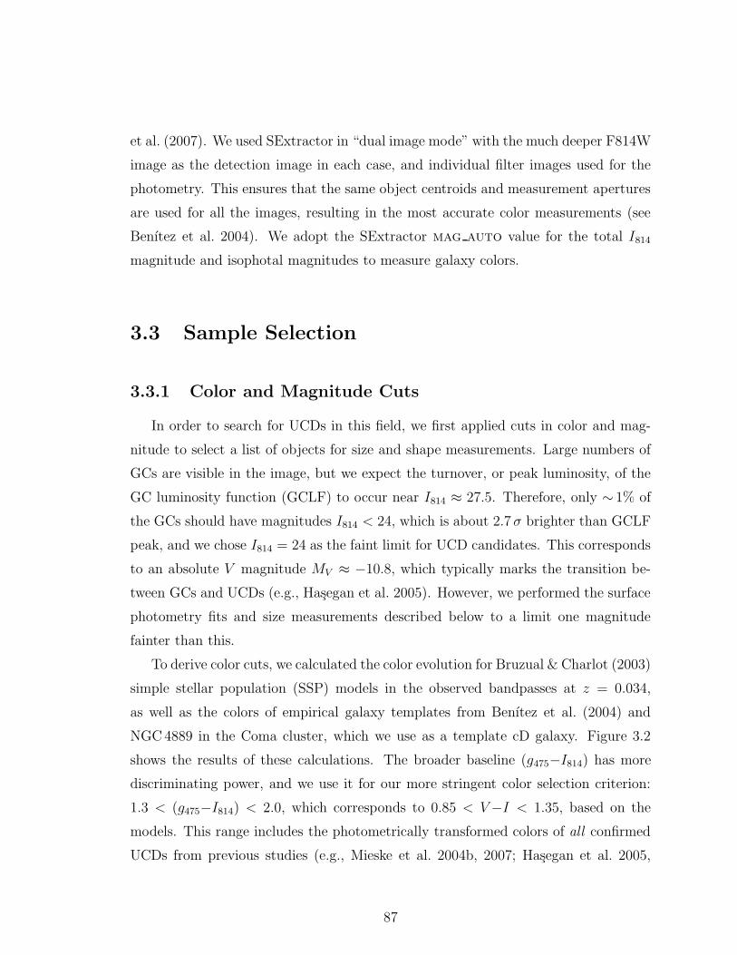
et al. (2007). We used SExtractor in “dual image mode” with the much deeper F814W
image as the detection image in each case, and individual filter images used for the
photometry. This ensures that the same object centroids and measurement apertures
are used for all the images, resulting in the most accurate color measurements (see
Benıtez et al. 2004). We adopt the SExtractor mag auto value for the total I814
magnitude and isophotal magnitudes to measure galaxy colors.
3.3 Sample Selection
3.3.1 Color and Magnitude Cuts
In order to search for UCDs in this field, we first applied cuts in color and mag-
nitude to select a list of objects for size and shape measurements. Large numbers of
GCs are visible in the image, but we expect the turnover, or peak luminosity, of the
GC luminosity function (GCLF) to occur near I814 ≈ 27.5. Therefore, only ∼ 1% of
the GCs should have magnitudes I814 < 24, which is about 2.7σ brighter than GCLF
peak, and we chose I814 = 24 as the faint limit for UCD candidates. This corresponds
to an absolute V magnitude MV ≈ −10.8, which typically marks the transition be-
tween GCs and UCDs (e.g., Hasegan et al. 2005). However, we performed the surface
photometry fits and size measurements described below to a limit one magnitude
fainter than this.
To derive color cuts, we calculated the color evolution for Bruzual & Charlot (2003)
simple stellar population (SSP) models in the observed bandpasses at z = 0.034,
as well as the colors of empirical galaxy templates from Benıtez et al. (2004) and
NGC4889 in the Coma cluster, which we use as a template cD galaxy. Figure 3.2
shows the results of these calculations. The broader baseline (g475−I814) has more
discriminating power, and we use it for our more stringent color selection criterion:
1.3 < (g475−I814) < 2.0, which corresponds to 0.85 < V −I < 1.35, based on the
models. This range includes the photometrically transformed colors of all confirmed
UCDs from previous studies (e.g., Mieske et al. 2004b, 2007; Hasegan et al. 2005,
87
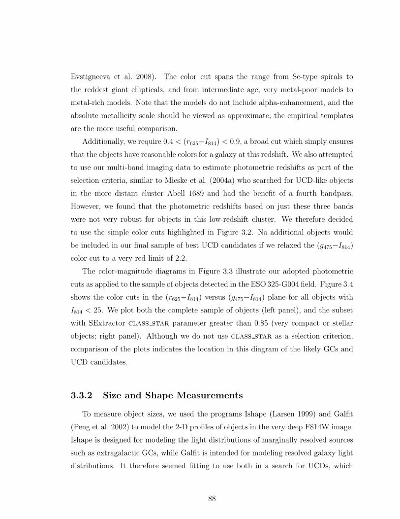
Evstigneeva et al. 2008). The color cut spans the range from Sc-type spirals to
the reddest giant ellipticals, and from intermediate age, very metal-poor models to
metal-rich models. Note that the models do not include alpha-enhancement, and the
absolute metallicity scale should be viewed as approximate; the empirical templates
are the more useful comparison.
Additionally, we require 0.4 < (r625−I814) < 0.9, a broad cut which simply ensures
that the objects have reasonable colors for a galaxy at this redshift. We also attempted
to use our multi-band imaging data to estimate photometric redshifts as part of the
selection criteria, similar to Mieske et al. (2004a) who searched for UCD-like objects
in the more distant cluster Abell 1689 and had the benefit of a fourth bandpass.
However, we found that the photometric redshifts based on just these three bands
were not very robust for objects in this low-redshift cluster. We therefore decided
to use the simple color cuts highlighted in Figure 3.2. No additional objects would
be included in our final sample of best UCD candidates if we relaxed the (g475−I814)
color cut to a very red limit of 2.2.
The color-magnitude diagrams in Figure 3.3 illustrate our adopted photometric
cuts as applied to the sample of objects detected in the ESO325-G004 field. Figure 3.4
shows the color cuts in the (r625−I814) versus (g475−I814) plane for all objects with
I814 < 25. We plot both the complete sample of objects (left panel), and the subset
with SExtractor class star parameter greater than 0.85 (very compact or stellar
objects; right panel). Although we do not use class star as a selection criterion,
comparison of the plots indicates the location in this diagram of the likely GCs and
UCD candidates.
3.3.2 Size and Shape Measurements
To measure object sizes, we used the programs Ishape (Larsen 1999) and Galfit
(Peng et al. 2002) to model the 2-D profiles of objects in the very deep F814W image.
Ishape is designed for modeling the light distributions of marginally resolved sources
such as extragalactic GCs, while Galfit is intended for modeling resolved galaxy light
distributions. It therefore seemed fitting to use both in a search for UCDs, which
88

Figure 3.2 Predicted age evolution in the observed ACS colors at redshift z=0.034 for
Bruzual & Charlot (2003) single-burst stellar population models with five different
metallicities, labeled by their [Fe/H] values. We also show the expected colors at
this redshift for six different empirical galaxy templates (see text) with arbitrary
placement along the horizontal axis. The shaded areas delineate the color selection
criteria for the UCD candidates. The broader baseline (g475−I814) color is used for
the more stringent selection cut, based on the expected range of stellar populations
in UCDs. The less-sensitive (r625−I814) cut is simply to ensure the objects have
reasonable colors for galaxies at this redshift.
89
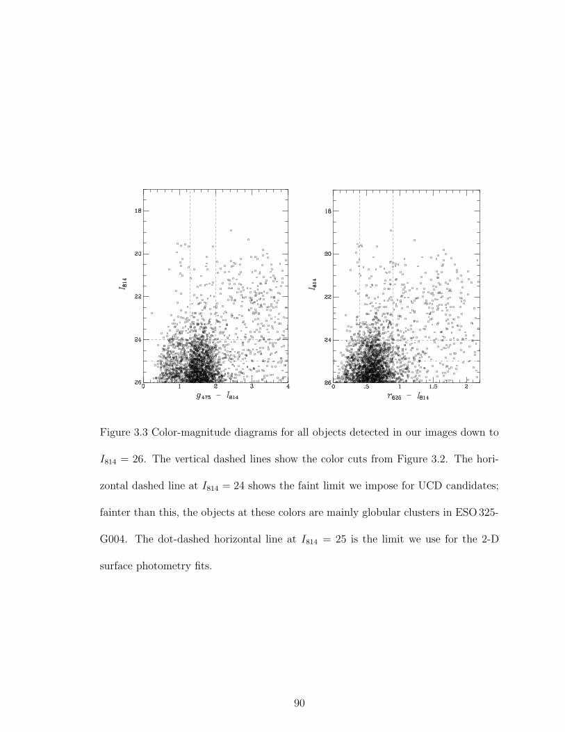
Figure 3.3 Color-magnitude diagrams for all objects detected in our images down to
I814 = 26. The vertical dashed lines show the color cuts from Figure 3.2. The hori-
zontal dashed line at I814 = 24 shows the faint limit we impose for UCD candidates;
fainter than this, the objects at these colors are mainly globular clusters in ESO325-
G004. The dot-dashed horizontal line at I814 = 25 is the limit we use for the 2-D
surface photometry fits.
90
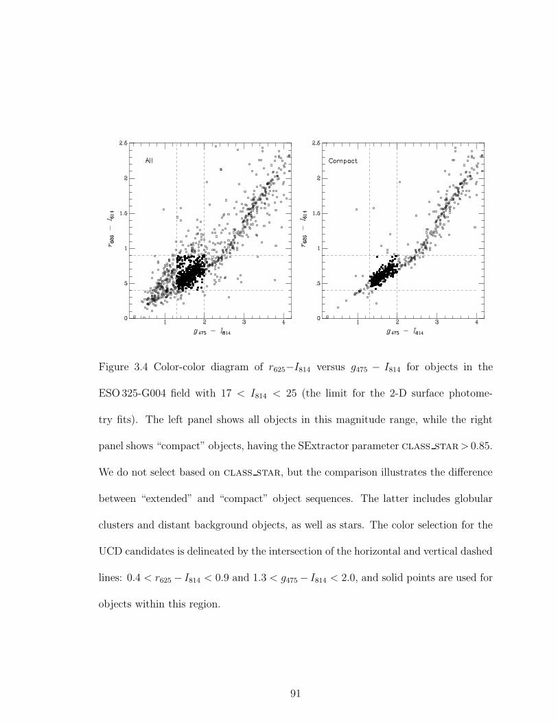
Figure 3.4 Color-color diagram of r625−I814 versus g475 − I814 for objects in the
ESO325-G004 field with 17 < I814 < 25 (the limit for the 2-D surface photome-
try fits). The left panel shows all objects in this magnitude range, while the right
panel shows “compact” objects, having the SExtractor parameter class star> 0.85.
We do not select based on class star, but the comparison illustrates the difference
between “extended” and “compact” object sequences. The latter includes globular
clusters and distant background objects, as well as stars. The color selection for the
UCD candidates is delineated by the intersection of the horizontal and vertical dashed
lines: 0.4 < r625 − I814 < 0.9 and 1.3 < g475 − I814 < 2.0, and solid points are used for
objects within this region.
91

straddle the range between GCs and dwarf galaxies. For the Ishape fits, we used the
“KING30” profile, a King (1962) model with concentration parameter c = 30, which
works well for marginally resolved GCs (e.g., Larsen & Brodie 2000). For Galfit, we
used a single Sersic (1968) model, which has one more degree of freedom than KING30.
Both programs are quite robust, with typical errors of 10-15% for compact but high
signal-to-noise sources such as we have here (see Blakeslee et al. 2006; Barber DeGraaff
et al. 2007). We fitted elliptical models, and use the circularized effective radius
Re,c = Re√
q = Re
√1 − ε, where Re is the effective radius along the major axis, q is
the fitted axis ratio, and ε is the ellipticity.
We modeled all objects in the field with 17 < I814 < 25, within the color ranges
given in § 3.3.1, and with SExtractor Kron radius ≤ 30 pix (1 kpc). The Kron
radius selection removes objects much larger than the UCD and compact elliptical
candidates that we are interested in; it should not exclude any objects in Abell S0740
with Sersic-like profiles and half light radii below ∼ 500 pc (see Graham & Driver
2005). Figure 3.5 shows the magnitude-size diagrams using the Re,c values from
Galfit (left panel) and Ishape (right panel), converted to parsecs using the adopted
distance. The two panels are similar in overall appearance, except Ishape resolves
many objects with Re,c < 10 pc (0.3 pix) that are not resolved by Galfit; these are
probably mainly globular clusters. In both cases, there are about a dozen bright,
unresolved objects (I814 < 23, Re,c = 0) that are most likely stars.
Figure 3.6 shows a direct comparison of Galfit and Ishape sizes for objects with
I814 < 24, the magnitude limit for our UCD candidate selection. To this limit, the
agreement is quite good, apart from the objects unresolved by Galfit (the agreement
worsens for fainter objects). Ishape does not do as well for the sizes of larger objects,
because it has a limited fit radius of only a few pixels and overestimates the sizes
of larger objects by about 50%. The two worst outliers among the objects that are
resolved by both software packages are irregular objects: #2228 is a blended double
source, and #575 is a bright clump within a larger edge-on galaxy. For the final list
of object sizes, we adopted the Galfit Re,c measurement if it was greater than 2 pix
(66 pc); otherwise, we used the Ishape value for Re,c.
Figure 3.7 plots the Sersic index n against Re,c from the Galfit Sersic model fits.
92

Figure 3.5 Magnitude-size diagrams for the selected sample of objects in the ESO325-
G004 field with I814 < 25 and the color cuts given in the preceding figures. We use
SExtractor mag auto for I814 and circular half-light radii Re,c from the Galfit Sersic
model (left) and Ishape King model (right) fits. Note that Re,c = Re,c
√1−ε , where
Re,c is the fitted half-light radius along the major axis, ε is the fitted ellipticity, and
(1−ε) the axis ratio. The image scale at the distance of ESO325-G004 is 33 pc pix−1 .
93
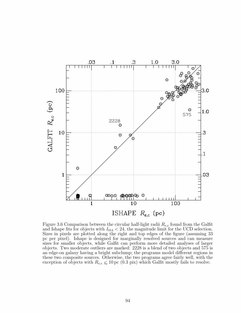
Figure 3.6 Comparison between the circular half-light radii Re,c found from the Galfitand Ishape fits for objects with I814 < 24, the magnitude limit for the UCD selection.Sizes in pixels are plotted along the right and top edges of the figure (assuming 33pc per pixel). Ishape is designed for marginally resolved sources and can measuresizes for smaller objects, while Galfit can perform more detailed analyses of largerobjects. Two moderate outliers are marked: 2228 is a blend of two objects and 575 isan edge-on galaxy having a bright subclump; the programs model different regions inthese two composite sources. Otherwise, the two programs agree fairly well, with theexception of objects with Re,c ∼< 10 pc (0.3 pix) which Galfit mostly fails to resolve.
94
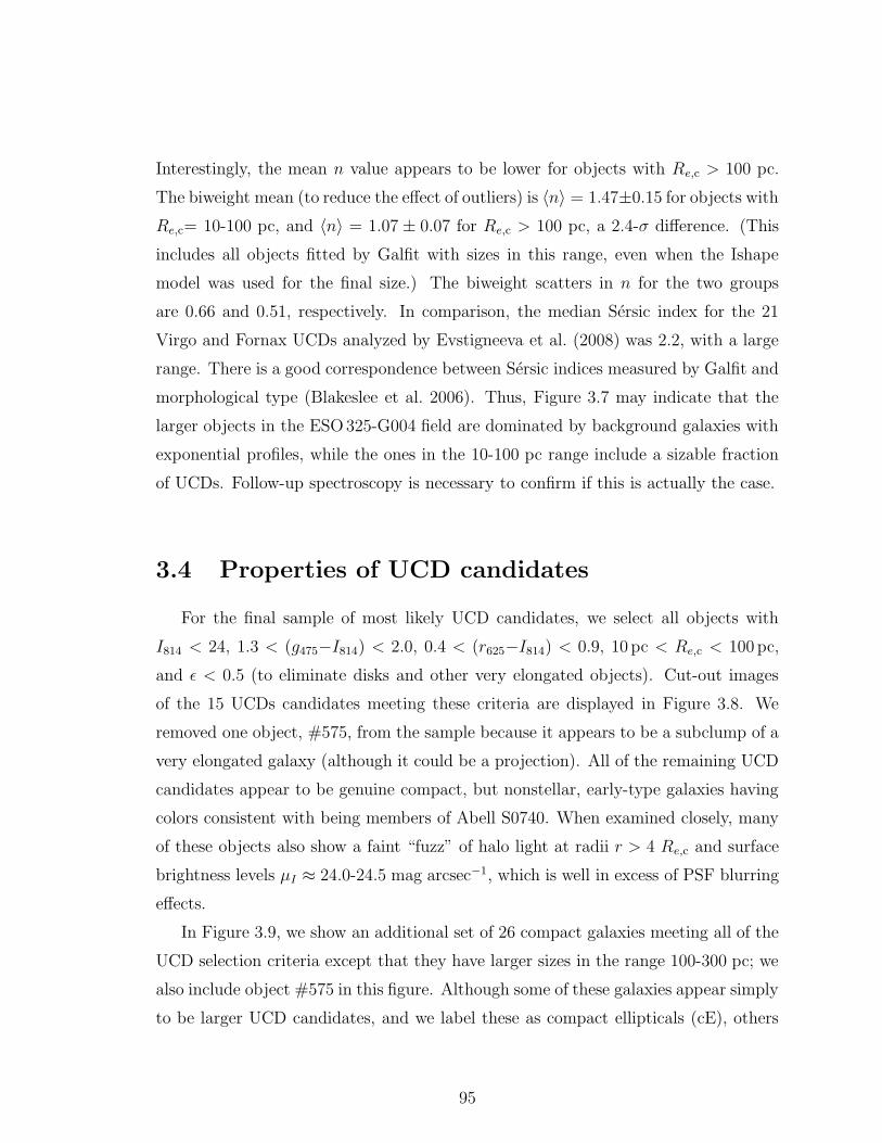
Interestingly, the mean n value appears to be lower for objects with Re,c > 100 pc.
The biweight mean (to reduce the effect of outliers) is 〈n〉 = 1.47±0.15 for objects with
Re,c= 10-100 pc, and 〈n〉 = 1.07 ± 0.07 for Re,c > 100 pc, a 2.4-σ difference. (This
includes all objects fitted by Galfit with sizes in this range, even when the Ishape
model was used for the final size.) The biweight scatters in n for the two groups
are 0.66 and 0.51, respectively. In comparison, the median Sersic index for the 21
Virgo and Fornax UCDs analyzed by Evstigneeva et al. (2008) was 2.2, with a large
range. There is a good correspondence between Sersic indices measured by Galfit and
morphological type (Blakeslee et al. 2006). Thus, Figure 3.7 may indicate that the
larger objects in the ESO325-G004 field are dominated by background galaxies with
exponential profiles, while the ones in the 10-100 pc range include a sizable fraction
of UCDs. Follow-up spectroscopy is necessary to confirm if this is actually the case.
3.4 Properties of UCD candidates
For the final sample of most likely UCD candidates, we select all objects with
I814 < 24, 1.3 < (g475−I814) < 2.0, 0.4 < (r625−I814) < 0.9, 10 pc < Re,c < 100 pc,
and ε < 0.5 (to eliminate disks and other very elongated objects). Cut-out images
of the 15 UCDs candidates meeting these criteria are displayed in Figure 3.8. We
removed one object, #575, from the sample because it appears to be a subclump of a
very elongated galaxy (although it could be a projection). All of the remaining UCD
candidates appear to be genuine compact, but nonstellar, early-type galaxies having
colors consistent with being members of Abell S0740. When examined closely, many
of these objects also show a faint “fuzz” of halo light at radii r > 4 Re,c and surface
brightness levels µI ≈ 24.0-24.5 mag arcsec−1, which is well in excess of PSF blurring
effects.
In Figure 3.9, we show an additional set of 26 compact galaxies meeting all of the
UCD selection criteria except that they have larger sizes in the range 100-300 pc; we
also include object #575 in this figure. Although some of these galaxies appear simply
to be larger UCD candidates, and we label these as compact ellipticals (cE), others
95

Figure 3.7 Sersic index n is plotted against the circularized half light radius Re,c for the
Galfit Sersic model fits. The dashed lines show the biweight mean values of 1.47±0.15
and 1.07 ± 0.07 for the objects with 10 < Re,c < 100 pc and 100 < Re,c < 400 pc,
respectively.
96
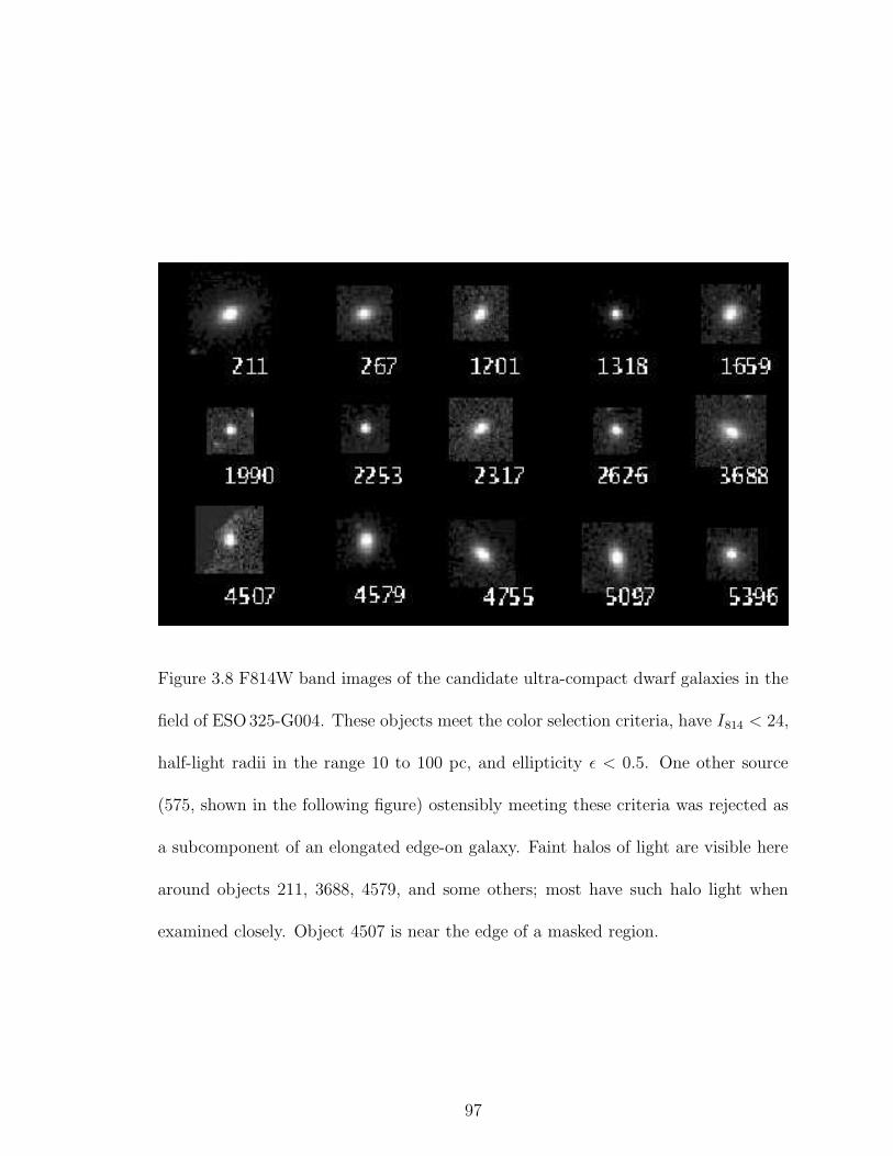
Figure 3.8 F814W band images of the candidate ultra-compact dwarf galaxies in the
field of ESO325-G004. These objects meet the color selection criteria, have I814 < 24,
half-light radii in the range 10 to 100 pc, and ellipticity ε < 0.5. One other source
(575, shown in the following figure) ostensibly meeting these criteria was rejected as
a subcomponent of an elongated edge-on galaxy. Faint halos of light are visible here
around objects 211, 3688, 4579, and some others; most have such halo light when
examined closely. Object 4507 is near the edge of a masked region.
97

are irregular galaxies, and a few appear to be small background spirals. Table 3.1 lists
the positions, magnitudes, colors, and sizes of the 41 objects in Figures 3.8 and 3.9.
Magnitudes and colors are corrected for extinction as described above. The last
column of Table 3.1 reports our classifications for these objects as UCD (all objects
in Fig. 3.8), cE, Sp (spiral), S0 (disky galaxy without obvious spiral structure), Irr
(irregular), or clump (subcomponent of an irregular or interacting system).
The ellipticity distributions of the 15 UCD candidates and other objects in the
field within the same magnitude and color ranges are shown in Figure 3.10. The
UCDs have a mean ε = 0.32 and a range from 0.16 to 0.46. The UCD sample
selection excludes objects with ε > 0.5, but it is interesting that none has ε ≤ 0.15.
This may reflect intrinsic flattening in the UCDs, since there are many objects in the
larger sample that are found to have lower ellipticity values.
Figure 3.11 shows the positions of the UCD candidates, larger compact galaxies,
globular clusters candidates with I814 < 25, and other objects in the field meeting our
color and magnitude cuts. Elliptical isophotes of ESO325-G004 are also drawn at
three radii. The galaxy is very regular. It has a mean ellipticity ε = 0.23±0.03 and is
oriented 45◦±2◦ counter-clockwise from the +x direction in the observed frame, which
translates to a position angle east of north of PA = 66◦ ± 2◦. (The errorbars reflect
the rms scatter among the fitted isophotes from the galaxy modeling in Sec. 3.2.) A
more detailed analysis of the GC population is in preparation, but we find a best-fit
PA = 71◦ ± 20◦ for the GC distribution, in close agreement with the major axis of
the galaxy isophotes. It is also noteworthy that 2/3 of the UCD candidates fall along
the galaxy’s major axis, within a region covering about 40% of the image. Although
not statistically very significant, the UCD alignment along this direction suggests a
link between the UCD and GC populations, and in turn with the stellar halo of the
central elliptical. We ran a 2-D Kolmogorov-Smirnov test and found that the spatial
distributions of the GCs and UCD candidates were at least consistent with being the
same. It will be important to see what fraction of the UCDs lie along the major axis
once a spectroscopically confirmed sample is available.
In the previous section, we examined the magnitude-size diagrams for the Re,c
values measured separately by Galfit and Ishape. Figure 3.12 presents our final
98

Figure 3.9 F814W band images of objects in the field of ESO325-G004 meeting all
the selection criteria for UCDs, except having slightly larger sizes in the range 100 to
300 pc (plus object 575, noted in the caption to Fig. 3.8). These objects are more
irregular in appearance; some appear to be background spiral galaxies.
99
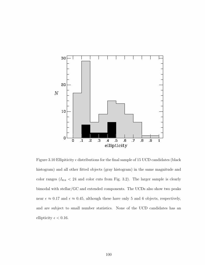
Figure 3.10 Ellipiticity ε distributions for the final sample of 15 UCD candidates (black
histogram) and all other fitted objects (gray histogram) in the same magnitude and
color ranges (I814 < 24 and color cuts from Fig. 3.2). The larger sample is clearly
bimodal with stellar/GC and extended components. The UCDs also show two peaks
near ε ≈ 0.17 and ε ≈ 0.45, although these have only 5 and 6 objects, respectively,
and are subject to small number statistics. None of the UCD candidates has an
ellipticity ε < 0.16.
100
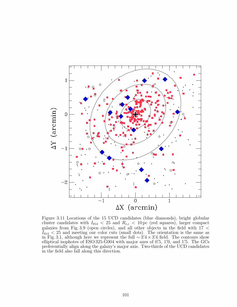
Figure 3.11 Locations of the 15 UCD candidates (blue diamonds), bright globularcluster candidates with I814 < 25 and Re,c < 10 pc (red squares), larger compactgalaxies from Fig. 3.9 (open circles), and all other objects in the field with 17 <I814 < 25 and meeting our color cuts (small dots). The orientation is the same asin Fig. 3.1, although here we represent the full ∼ 3.′4× 3.′4 field. The contours showelliptical isophotes of ESO325-G004 with major axes of 0.′5, 1.′0, and 1.′5. The GCspreferentially align along the galaxy’s major axis. Two-thirds of the UCD candidatesin the field also fall along this direction.
101
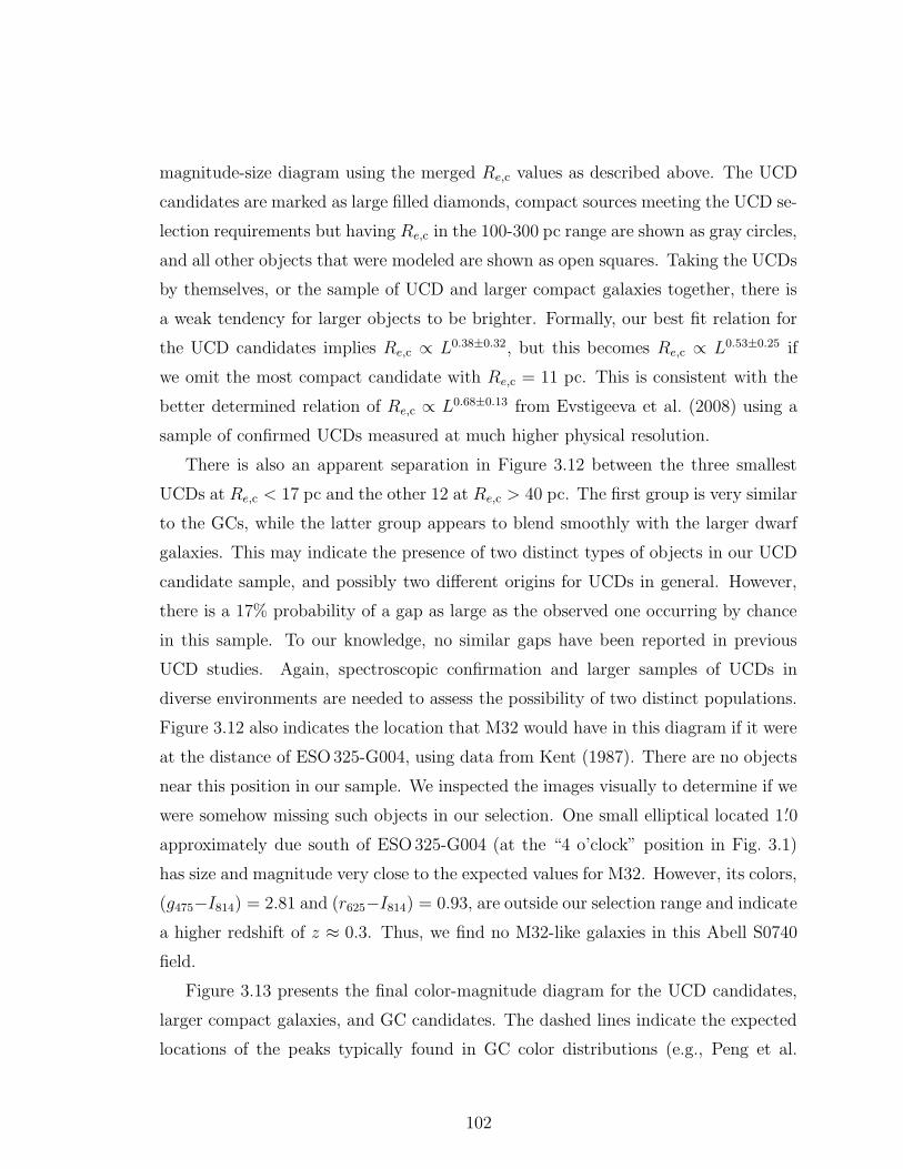
magnitude-size diagram using the merged Re,c values as described above. The UCD
candidates are marked as large filled diamonds, compact sources meeting the UCD se-
lection requirements but having Re,c in the 100-300 pc range are shown as gray circles,
and all other objects that were modeled are shown as open squares. Taking the UCDs
by themselves, or the sample of UCD and larger compact galaxies together, there is
a weak tendency for larger objects to be brighter. Formally, our best fit relation for
the UCD candidates implies Re,c ∝ L0.38±0.32, but this becomes Re,c ∝ L0.53±0.25 if
we omit the most compact candidate with Re,c = 11 pc. This is consistent with the
better determined relation of Re,c ∝ L0.68±0.13 from Evstigeeva et al. (2008) using a
sample of confirmed UCDs measured at much higher physical resolution.
There is also an apparent separation in Figure 3.12 between the three smallest
UCDs at Re,c < 17 pc and the other 12 at Re,c > 40 pc. The first group is very similar
to the GCs, while the latter group appears to blend smoothly with the larger dwarf
galaxies. This may indicate the presence of two distinct types of objects in our UCD
candidate sample, and possibly two different origins for UCDs in general. However,
there is a 17% probability of a gap as large as the observed one occurring by chance
in this sample. To our knowledge, no similar gaps have been reported in previous
UCD studies. Again, spectroscopic confirmation and larger samples of UCDs in
diverse environments are needed to assess the possibility of two distinct populations.
Figure 3.12 also indicates the location that M32 would have in this diagram if it were
at the distance of ESO325-G004, using data from Kent (1987). There are no objects
near this position in our sample. We inspected the images visually to determine if we
were somehow missing such objects in our selection. One small elliptical located 1.′0
approximately due south of ESO325-G004 (at the “4 o’clock” position in Fig. 3.1)
has size and magnitude very close to the expected values for M32. However, its colors,
(g475−I814) = 2.81 and (r625−I814) = 0.93, are outside our selection range and indicate
a higher redshift of z ≈ 0.3. Thus, we find no M32-like galaxies in this Abell S0740
field.
Figure 3.13 presents the final color-magnitude diagram for the UCD candidates,
larger compact galaxies, and GC candidates. The dashed lines indicate the expected
locations of the peaks typically found in GC color distributions (e.g., Peng et al.
102
Figure 3.12 F814W magnitude versus size for UCD candidates (filled diamonds),larger compact galaxies in the 100-300 pc range (circles) and all other objects (opensquares) in the ESO325-G004 field that meet our color selection criteria and arewithin the plotted magnitude and size limits. Objects with Re,c < 10 pc are designatedglobular cluster candidates, while the UCD candidates are chosen as having Re,c = 10to 100 pc and ellipticity < 0.5. However, there may be a separation between the mostcompact UCD candidates with Re,c < 20 pc, similar to large globular clusters, andthose with Re,c ∼> 40 pc, which may be true compact dwarfs. Completely unresolvedobjects with Re,c ≈ 0 fall off the edge of this logarithmic plot. We show the expectedlocation for M32 at this distance; no similar galaxies are found in our sample.
103

2006). Past studies have found that UCDs tended to be slightly redder than the
average for the GC population (Wehner & Harris 2007; Evstigneeva et al. 2008).
Wehner & Harris described the color-magnitude sequence for their (unresolved) UCD
candidates as an extension of the red GC subpopulation to higher luminosities. We
also find that the UCDs in Figure 3.13 are weighted towards redder colors, especially
the brightest ones. We note that several of the compact galaxies with Re,c > 100
pc fall intriguingly close to the expected peaks of the GC color distribution, but the
interpretation for these objects is unclear until we have spectroscopic redshifts.
The ∼ 3.′4× 3.′4 coverage of our images translates to about 125× 125 kpc. We
find that our sample of 15 UCD candidates is reasonable compared with the numbers
found over similar magnitude limits in other clusters. In the Fornax cluster, only 4
objects are found within a similar radius of NGC1399 (Mieske et al. 2004b; Jones
et al. 2006). The number in Virgo is complicated by the enormous GC population
around M87, and the lack of a complete high-resolution imaging survey of the core
region. Jones et al. (2006) and Evstigneeva et al. (2008) indicate ∼ 5 UCDs within
this distance of M87, but an additional five were found by Hasegan et al. (2005)
in a physical area 70 times smaller than our own. Therefore, there may be dozens
of UCDs clustered close to M87. Perhaps the most comparable survey to ours is
that by Wehner & Harris (2007) who tabulated 29 UCD candidates in a 5.′5 field in
the center of the Hydra cluster, to about the same absolute magnitude limit. The
physical area covered by their imaging is roughly half of ours; so, we might expect
to find ∼ 60 candidates based on this extrapolation. However, Wehner & Harris used
ground-based imaging and were not able to select based on objects sizes; if we had not
made the lower Re,c size cut, we would have a much larger sample of 58 candidates,
although the majority of these would be stars and bright GCs. We also note that our
sample size is roughly comparable to the numbers within similar radii in the “Fornax”
and “Virgo” numerical models presented by Bekki et al. (2003).
Finally, we provide estimates of the stellar masses of the UCD candidates and
compact galaxies in Figures 3.8 and 3.9. We calculated the masses of each of the
candidates using relations between mass-to-light ratio M/LV and (g475−I814) based
on the SSP models from Figure 3.2. The M/LV values we find for the UCD candidates
104

Figure 3.13 Color-magnitude diagram for UCD candidates (diamonds), globular clus-ter candidates (small squares) and larger compact galaxies from Fig. 3.9 (circles).The dashed lines indicate the expected locations of the characteristic peaks in theglobular cluster color distribution. The UCD candidates are weighted toward the redpeak location. It is interesting that most of the brightest larger objects (circles atI814 ∼< 22.8) lie near the dashed lines. The bright objects marked as globular clustercandidates (squares at I814 ∼< 22.8) are all unresolved and may be predominantly stars(they all fall off the left edge of Fig. 3.12).
105
range from ∼ 0.5 to 3.5, which are likely uncertain by about 30-50%, based on the
scatter in the models. The same uncertainty is inherent in the stellar mass estimates,
which we give in Table 3.1. The values for the UCD candidates range from 6×10⁶ to
108 M�, with a median of 3.4×10⁷ M�. This agrees well with the dynamically derived
masses of ∼ (2-9)× 107 M� from Evstigneeva et al. 2007a, a range that includes 73%
of our candidates. Similarly, Hilker et al. (2007) found dynamical masses of 1.8 to
9.5× 10⁷ M� for five bright Fornax UCDs. The two objects with the largest masses
in Table 3.1 (#419 and #4883) have Re,c values too large for inclusion in the UCD
sample, and both have structure indicating they are probably background objects
(see Fig. 3.9). We conclude that our mass estimates are reasonable for UCDs.
3.5 Summary
We have presented an analysis of three-band ACS/WFC imaging to search for
possible UCDs near the lensing galaxy ESO325-G004 in Abell S0740. This is an
interesting target for a UCD search because it is a massive central elliptical in a
poor cluster environment with a velocity dispersion similar to that of Fornax. We
selected objects based on their having magnitudes brighter than 99% of the expected
GCs population, color appropriate for an early-type or population II system at this
redshift, ellipticity less than 0.5, and circular half-light radii in the 10-100 pc range.
The radii were measured using both the Galfit and Ishape programs. We found 15
good UCD candidates meeting the selection criteria, comparable to the expectations
from previous searches.
In addition, we presented a sample of larger compact galaxies with radii in the
range 100-300 pc, if they are located within the cluster. These objects appear to
be a mix of irregular background galaxies and larger versions of the cluster UCDs.
We did not find any counterparts of M32 in this field. The mean Sersic index for
the UCD candidates is around 1.5, which is marginally higher than the value ∼ 1
found for the larger compact galaxies. This may indicate that the latter objects
are dominated by background disk-like galaxies, while the former group is mainly
106

comprised of UCDs in the cluster. Most of the UCD candidates and larger compact
galaxies have visible surrounding halo light, consistent with galaxy threshing models.
There is also evidence that most UCDs are intrinsically flattened, as none of the 15
UCD candidates has a fitted ellipticity ε < 0.16.
The magnitude-size and color-magnitude diagrams show general continuity in the
distributions of these parameters from GCs to the UCDs candidates. For our limited
sample of UCD candidates, we find Re,c ∼ L0.5. This is an intriguing proportionality,
as it implies a roughly constant surface brightness for UCDs of different sizes. The
better determined relation from Evstigneeva et al. (2008) is somewhat steeper, but
consistent within the errors. There may be a bifurcation in the UCDs between those
with sizes similar to GCs and larger ones with Re,c > 40 pc, suggesting different
origins for these two groups. However, because of the small number of objects, the
significance of the observed gap in Re,c is only 83%. Therefore, although suggestive,
it remains inconclusive. The colors of UCD candidates are weighted towards the red
compared to the expected (g475−I814) GC color distribution. Several of the bright
compact galaxies with sizes in the 100-300 pc range have colors near the expected
peaks of the GC color distribution. It would be useful to know if these objects are
also in the cluster, and what may be their relation to the UCDs.
The majority of UCD candidates align along the major axis of ESO325-G004,
similar to the spatial distribution of the bright GCs. Because of the small numbers
involved, this result is not highly significant, but follow-up spectroscopy can provide
a confirmed sample of UCDs; it will be interesting to see if these are mainly along the
galaxy’s major axis. These findings may appear to support a scenario in which the
UCDs are the high-luminosity extension of the GC system. However, as discussed in
the Introduction, the true situation is probably more complex, and many red GCs
may actually have their origin as stripped nucleated dwarfs, clouding the distinction
between the main UCD formation scenarios. It would be useful to discover how
the number of UCDs in complete surveys of many different clusters scales with the
GC population of the central galaxy. We are currently completing a more detailed
analysis of the GC population in this cluster and other similar fields from the same
HST program. We also plan to obtain spectroscopy for all our UCD candidates to
107

see what fraction of them are indeed associated with ESO325-G004. The additional
information from these studies should provide further insight into the origin of UCDs
and their connection to the GC populations.
108
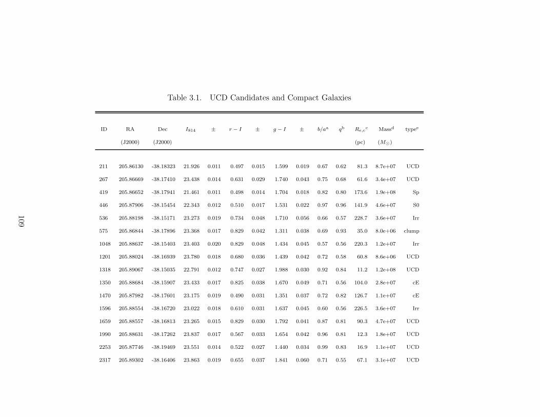
Table 3.1. UCD Candidates and Compact Galaxies
ID RA Dec I814 ± r − I ± g − I ± b/aa qb Re,cc Massd typee
(J2000) (J2000) (pc) (M�)
211 205.86130 -38.18323 21.926 0.011 0.497 0.015 1.599 0.019 0.67 0.62 81.3 8.7e+07 UCD
267 205.86669 -38.17410 23.438 0.014 0.631 0.029 1.740 0.043 0.75 0.68 61.6 3.4e+07 UCD
419 205.86652 -38.17941 21.461 0.011 0.498 0.014 1.704 0.018 0.82 0.80 173.6 1.9e+08 Sp
446 205.87906 -38.15454 22.343 0.012 0.510 0.017 1.531 0.022 0.97 0.96 141.9 4.6e+07 S0
536 205.88198 -38.15171 23.273 0.019 0.734 0.048 1.710 0.056 0.66 0.57 228.7 3.6e+07 Irr
575 205.86844 -38.17896 23.368 0.017 0.829 0.042 1.311 0.038 0.69 0.93 35.0 8.0e+06 clump
1048 205.88637 -38.15403 23.403 0.020 0.829 0.048 1.434 0.045 0.57 0.56 220.3 1.2e+07 Irr
1201 205.88024 -38.16939 23.780 0.018 0.680 0.036 1.439 0.042 0.72 0.58 60.8 8.6e+06 UCD
1318 205.89067 -38.15035 22.791 0.012 0.747 0.027 1.988 0.030 0.92 0.84 11.2 1.2e+08 UCD
1350 205.88684 -38.15907 23.433 0.017 0.825 0.038 1.670 0.049 0.71 0.56 104.0 2.8e+07 cE
1470 205.87982 -38.17601 23.175 0.019 0.490 0.031 1.351 0.037 0.72 0.82 126.7 1.1e+07 cE
1596 205.88554 -38.16720 23.022 0.018 0.610 0.031 1.637 0.045 0.60 0.56 226.5 3.6e+07 Irr
1659 205.88557 -38.16813 23.265 0.015 0.829 0.030 1.792 0.041 0.87 0.81 90.3 4.7e+07 UCD
1990 205.88631 -38.17262 23.837 0.017 0.567 0.033 1.654 0.042 0.96 0.81 12.3 1.8e+07 UCD
2253 205.87746 -38.19469 23.551 0.014 0.522 0.027 1.440 0.034 0.99 0.83 16.9 1.1e+07 UCD
2317 205.89302 -38.16406 23.863 0.019 0.655 0.037 1.841 0.060 0.71 0.55 67.1 3.1e+07 UCD
109

Table 3.1 (cont’d)
ID RA Dec I814 ± r − I ± g − I ± b/aa qb Re,cc Massd typee
(J2000) (J2000) (pc) (M�)
2445 205.87746 -38.19764 23.264 0.018 0.579 0.032 1.522 0.045 0.53 0.58 178.2 1.9e+07 Irr
2626 205.89274 -38.16961 23.594 0.016 0.660 0.031 1.372 0.034 0.88 0.70 40.0 7.9e+06 UCD
2632 205.89377 -38.16771 23.947 0.033 0.876 0.087 1.503 0.093 0.51 0.56 241.5 9.5e+06 Irr
3153 205.88536 -38.19365 21.912 0.012 0.499 0.016 1.413 0.020 0.87 0.66 211.8 4.4e+07 Irr
3495 205.90039 -38.16848 23.638 0.021 0.692 0.043 1.665 0.059 0.73 0.59 142.2 2.3e+07 Irr
3688 205.89787 -38.17786 22.535 0.015 0.640 0.022 1.695 0.034 0.77 0.54 90.2 6.9e+07 UCD
4054 205.89599 -38.19076 23.541 0.018 0.549 0.033 1.330 0.041 0.75 0.80 128.1 7.2e+06 Sp
4062 205.91205 -38.15832 22.308 0.011 0.554 0.022 1.729 0.024 0.76 0.65 109.9 9.4e+07 cE
4171 205.91251 -38.16059 23.294 0.015 0.513 0.037 1.630 0.042 0.73 0.62 108.6 2.7e+07 cE
4441 205.90959 -38.17646 20.721 0.010 0.531 0.012 1.405 0.013 0.78 0.76 257.2 1.3e+08 Sp/Irr
4507 205.90258 -38.19380 23.979 0.020 0.664 0.044 1.397 0.052 0.68 0.54 44.1 6.1e+06 UCD
4510 205.91878 -38.16098 22.464 0.012 0.795 0.029 1.964 0.035 0.50 0.56 131.6 1.5e+08 cE
4513 205.92092 -38.15667 23.897 0.028 0.543 0.075 1.575 0.083 0.85 0.89 219.5 1.3e+07 Irr
4579 205.91782 -38.16729 22.154 0.011 0.767 0.017 1.647 0.020 0.76 0.77 80.2 8.3e+07 UCD
4616 205.90719 -38.19038 23.969 0.026 0.625 0.055 1.763 0.084 0.85 0.90 129.3 2.3e+07 clump
4755 205.91962 -38.17162 22.799 0.012 0.534 0.020 1.569 0.028 0.73 0.54 76.4 3.5e+07 UCD
110
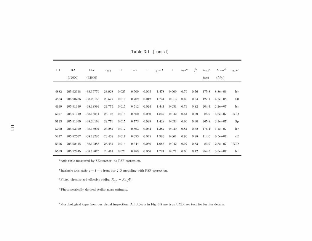
Table 3.1 (cont’d)
ID RA Dec I814 ± r − I ± g − I ± b/aa qb Re,cc Massd typee
(J2000) (J2000) (pc) (M�)
4882 205.92918 -38.15779 23.928 0.025 0.509 0.065 1.478 0.069 0.79 0.76 175.8 8.8e+06 Irr
4883 205.90786 -38.20153 20.577 0.010 0.709 0.012 1.734 0.013 0.69 0.54 127.1 4.7e+08 S0
4930 205.91646 -38.18593 22.775 0.015 0.512 0.024 1.441 0.031 0.73 0.82 204.4 2.2e+07 Irr
5097 205.91919 -38.18841 23.193 0.014 0.860 0.030 1.832 0.042 0.64 0.59 85.9 5.6e+07 UCD
5123 205.91309 -38.20199 22.776 0.015 0.773 0.029 1.428 0.033 0.90 0.90 265.8 2.1e+07 Sp
5200 205.93059 -38.16994 23.284 0.017 0.863 0.054 1.387 0.040 0.84 0.62 176.4 1.1e+07 Irr
5247 205.92507 -38.18285 23.438 0.017 0.693 0.045 1.983 0.061 0.93 0.98 114.0 6.5e+07 cE
5396 205.92415 -38.19283 23.454 0.014 0.544 0.036 1.683 0.042 0.92 0.83 83.9 2.8e+07 UCD
5503 205.92445 -38.19675 23.414 0.023 0.489 0.056 1.721 0.071 0.66 0.72 254.5 3.3e+07 Irr
aAxis ratio measured by SExtractor; no PSF correction.
bIntrinsic axis ratio q = 1 − ε from our 2-D modeling with PSF correction.
cFitted circularized effective radius Re,c = Re√
q.
dPhotometrically derived stellar mass estimate.
eMorphological type from our visual inspection. All objects in Fig. 3.8 are type UCD; see text for further details.
111

Bibliography
[1] Abell, G. O. 1958, ApJS, 3, 211
[2] Abell, G. O., Corwin, H. G., Jr., & Olowin, R. P. 1989, ApJS, 70, 1
[3] Barber DeGraaff, R., Blakeslee, J. P., Meurer, G. R., & Putman, M. E. 2007,
ApJ, 671, 1624
[4] Bassino, L. P., Muzzio, J. C., & Rabolli, M. 1994, ApJ, 431, 634
[5] Bekki, K. 2007, MNRAS, 380, 1177
[6] Bekki, K., Couch, W. J., & Drinkwater, M. J. 2001, ApJ, 552, L105
[7] Bekki, K., Couch, W. J., Drinkwater, M. J., & Shioya, Y. 2003, MNRAS, 344,
399
[8] Benıtez, N., et al. 2004, ApJS, 150, 1
[4] Bertin, E., & Arnouts, S. 1996, A&AS, 117, 393
[10] Blakeslee, J. P. 2007, Cosmic Frontiers, ASP Conference Series, 379, 99
[4] Blakeslee, J. P., Anderson, K. R., Meurer, G. R., Benıtez, N., & Magee, D. 2003,
Astronomical Data Analysis Software and Systems XII, 295, 257
[12] Blakeslee, J. P., et al. 2006, ApJ, 644, 30
[13] Bruzual, G. & Charlot, S. 2003, MNRAS, 344, 1000
112
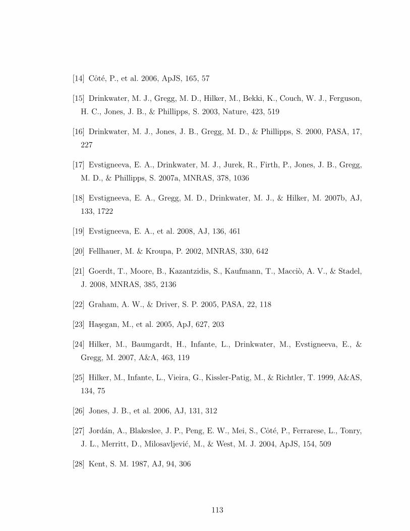
[14] Cote, P., et al. 2006, ApJS, 165, 57
[15] Drinkwater, M. J., Gregg, M. D., Hilker, M., Bekki, K., Couch, W. J., Ferguson,
H. C., Jones, J. B., & Phillipps, S. 2003, Nature, 423, 519
[16] Drinkwater, M. J., Jones, J. B., Gregg, M. D., & Phillipps, S. 2000, PASA, 17,
227
[17] Evstigneeva, E. A., Drinkwater, M. J., Jurek, R., Firth, P., Jones, J. B., Gregg,
M. D., & Phillipps, S. 2007a, MNRAS, 378, 1036
[18] Evstigneeva, E. A., Gregg, M. D., Drinkwater, M. J., & Hilker, M. 2007b, AJ,
133, 1722
[19] Evstigneeva, E. A., et al. 2008, AJ, 136, 461
[20] Fellhauer, M. & Kroupa, P. 2002, MNRAS, 330, 642
[21] Goerdt, T., Moore, B., Kazantzidis, S., Kaufmann, T., Maccio, A. V., & Stadel,
J. 2008, MNRAS, 385, 2136
[22] Graham, A. W., & Driver, S. P. 2005, PASA, 22, 118
[23] Hasegan, M., et al. 2005, ApJ, 627, 203
[24] Hilker, M., Baumgardt, H., Infante, L., Drinkwater, M., Evstigneeva, E., &
Gregg, M. 2007, A&A, 463, 119
[25] Hilker, M., Infante, L., Vieira, G., Kissler-Patig, M., & Richtler, T. 1999, A&AS,
134, 75
[26] Jones, J. B., et al. 2006, AJ, 131, 312
[27] Jordan, A., Blakeslee, J. P., Peng, E. W., Mei, S., Cote, P., Ferrarese, L., Tonry,
J. L., Merritt, D., Milosavljevic, M., & West, M. J. 2004, ApJS, 154, 509
[28] Kent, S. M. 1987, AJ, 94, 306
113

[14] King, I. 1962, AJ, 67, 471
[30] Larsen, S. S. 1999, A&AS, 139, 393
[31] Larsen, S. S., & Brodie, J. P. 2000, AJ, 120, 2938
[32] Mieske, S., Hilker, M., & Infante, L. 2002, A&A, 383, 823
[33] Mieske, S., Hilker, M., & Infante, L. 2004b, A&A, 418, 445
[34] Mieske, S., Hilker, M., Infante, L., & Jordan, A. 2006, AJ, 131, 2442
[35] Mieske, S., Hilker, M., Jordan, A., Infante, L., & Kissler-Patig, M. 2007, A&A,
472, 111
[36] Mieske, S., et al. 2004a, AJ, 128, 1529
[37] Peng, C. Y., Ho, L. C., Impey, C. D., & Rix, H. 2002, AJ, 124, 266
[9] Peng, E. W., Jordan, A., Cote, P., Blakeslee, J P., Ferrarese, L., Mei, S., West,
M. J., Merritt, D., Milosavljevic, M., & Tonry, J. L. 2006, ApJ, 639, 95
[39] Phillipps, S., Drinkwater, M. J., Gregg, M. D., & Jones, J. B. 2001, ApJ, 560,
201
[Schlegel et al. 1998] Schlegel, D. J., Finkbeiner, D. P., & Davis, M. 1998, ApJ, 500,
525
[40] Sersic, J. L. 1968, Atlas de Galaxias Australes (Cordoba: Observatorio Astro-
nomico)
[41] Sirianni, M., et al. 2005, PASP, 117, 1049
[17] Smith, R. J., Blakeslee, J. P., Lucey, J. R., & Tonry, J. 2005, ApJ, 625, L103
[43] Spergel, D. N., et al. 2007, ApJS, 170, 377
[44] Thomas, P. A., Drinkwater, M. J., & Evstigneeva, E. 2008, MNRAS, 389, 102
114

[45] Tonry, J. L., Blakeslee, J. P., Ajhar, E. A., & Dressler, A. 1997, ApJ, 475, 399
[46] Wehner, E. M. H. & Harris, W. E. 2007, ApJ, 668, L35
115

Chapter 4
Introduction to the Shapley
Supercluster and Data Analysis
The work presented in Chapters 4, 5 and 6 was undertaken in collaboration with
Dr. John Blakeslee. The DAOphot analysis in this chapter was also undertaken in
collaboration with Dr. William Harris.
4.1 Motivation for Survey Data
In January 2005, the HST GO Program 10429 obtained F814W band imaging
of 11 galaxies in the Shapley Supercluster. To better understand the motivations of
this program, we must first discuss the location and motions of the local cluster of
galaxies to which the Milky Way belongs.
116
4.1.1 Local Group Motion
The Local Group consists of a cluster of about 30 gravitationally bound galaxy
members with the Milky Way galaxy as the second largest member and the An-
dromeda Galaxy, M31, being the largest. The membership criterion is being within
a radial distance of 1.5 Mpc (∼ 5 million light years) of the cluster’s center between
the Milky Way and M31. Membership is vague, and has been updated in recent years
(van den Berg, 2000). This update is due to the Local Group being gravitationally
bound to other nearby groups and by the difficulty in knowing what members are
free to leave the bound Local Group. In Chapter 1, we discussed Hubble’s Law and
the motion of the galaxies in the universe. However, there are deviations from the
Hubble Flow called peculiar velocities. These peculiar velocities result from the influ-
ence of nearby mass concentrations. The nearest large cluster of galaxies, the Virgo
cluster, creates a motion in a direction apart from the expected Hubble expansion,
of 250km/s. This is called the Virgocentric infall. The Local Group and the Virgo
cluster are members of a larger bound group called the Local Supercluster, where
Virgo is more concentrated at the Local Supercluster’s center and the Local Group
is located in a more outlying region (Binney 1998).
4.1.2 Great Attractor
A more significant departure from the Hubble flow is a velocity of about 600km/s
motion relative to the Cosmic Radiation Background (CMB) our local group of galax-
ies experiences. To explain this motion, astronomers speculated the cause to be a huge
concentration of mass in the direction of Centaurus and called it the Great Attractor.
It was initially hard to investigate due to the fact that Centaurus lies close to the
Milky Way’s galactic plane where there is a large amount of extinction from dust.
The Hydra-Centaurus supercluster was ruled out as the Great Attractor in Lynden-
Bell et al. (1988). They concluded that the primary source of this ∼ 600km/s motion
was 40% further away. Lynden-Bell et al. also found that the Hydra-Centaurus su-
percluster was, itself, falling toward the Great Attractor at velocities greater than
117

1000 km/s. This finding remains a controversial finding and the identity of the Great
Attractor is still debated. HST GO Program 10429 was submitted to investigate a
large mass concentration in the direction of Centaurus, the Shapley Supercluster.
4.1.3 Shapley Supercluster
Located in the Southern Hemisphere and centered at a distance of ∼ 150-200 Mpc
(490-650 million light years), the Shapley Supercluster (SSC) constitutes the densest
part of the nearby universe. First discovered in 1930 by Harlow Shapley during a
survey of galaxies in the southern hemisphere, he mentions a cloud of galaxies in
Centaurus that appears to be the most populous yet discovered. Figure 4.1 gives a
good visual representation of SSC’s distance from the Milky Way and the distribution
of the cluster members. It is the richest supercluster in the direction (and distance) of
the Great Attractor. If the peculiar velocities for SSC members can be calculated then
a more accurate mass density map can be created for the SSC. Also this survey’s main
goal was to obtain SBF distances to several galaxies within the SSC, which recently
became possible because of the ACS (section 4.3.1). This data was also intended to
be used to further the study of globular clusters in this rich, dense environment.
The following is a list of the clusters targeted and the galaxy members imaged:
A1736a: ESO509-g008, ESO509-g020, ESO509-g067
A3558: ESO444-g046, 2masxj13275493-3132187 (PGC47197),
2masxj13272961-3123237 (PGC47154), 2masxj13280261-3145207 (PGC88857)
A3571: ESO383-g076, 2masxj13481399-3322547 (PGC84052)
A3570: ESO325-g016 & AS0740: ESO325-g004
The galaxies with names that begin with 2masxj will further be simplified in this
study as 2mj with the last 7 digits left off. For example, 2masxj13275493-313287
will be called 2mj13275493. Table 4.1 is a list containing a few galaxy properties,
obtained from various sources, of each of the 11 galaxies in this study. The first
and second columns are the name of the galaxy and cluster the galaxy belongs to,
respectively. The next two columns are the right ascension (RA) and declination
(Dec). The following column is the class of galaxy obtained from the NASA/IPAC
118
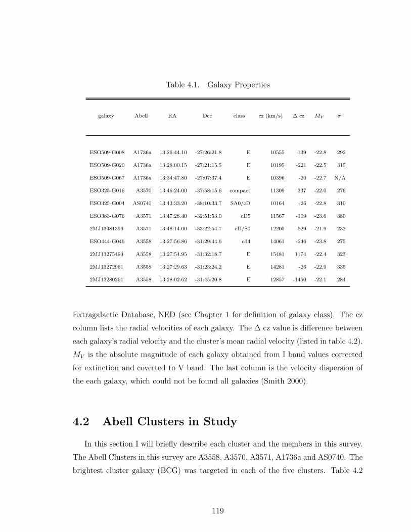
Table 4.1. Galaxy Properties
galaxy Abell RA Dec class cz (km/s) ∆ cz MV σ
ESO509-G008 A1736a 13:26:44.10 -27:26:21.8 E 10555 139 -22.8 292
ESO509-G020 A1736a 13:28:00.15 -27:21:15.5 E 10195 -221 -22.5 315
ESO509-G067 A1736a 13:34:47.80 -27:07:37.4 E 10396 -20 -22.7 N/A
ESO325-G016 A3570 13:46:24.00 -37:58:15.6 compact 11309 337 -22.0 276
ESO325-G004 AS0740 13:43:33.20 -38:10:33.7 SA0/cD 10164 -26 -22.8 310
ESO383-G076 A3571 13:47:28.40 -32:51:53.0 cD5 11567 -109 -23.6 380
2MJ13481399 A3571 13:48:14.00 -33:22:54.7 cD/S0 12205 529 -21.9 232
ESO444-G046 A3558 13:27:56.86 -31:29:44.6 cd4 14061 -246 -23.8 275
2MJ13275493 A3558 13:27:54.95 -31:32:18.7 E 15481 1174 -22.4 323
2MJ13272961 A3558 13:27:29.63 -31:23:24.2 E 14281 -26 -22.9 335
2MJ13280261 A3558 13:28:02.62 -31:45:20.8 E 12857 -1450 -22.1 284
Extragalactic Database, NED (see Chapter 1 for definition of galaxy class). The cz
column lists the radial velocities of each galaxy. The ∆ cz value is difference between
each galaxy’s radial velocity and the cluster’s mean radial velocity (listed in table 4.2).
MV is the absolute magnitude of each galaxy obtained from I band values corrected
for extinction and coverted to V band. The last column is the velocity dispersion of
the each galaxy, which could not be found all galaxies (Smith 2000).
4.2 Abell Clusters in Study
In this section I will briefly describe each cluster and the members in this survey.
The Abell Clusters in this survey are A3558, A3570, A3571, A1736a and AS0740. The
brightest cluster galaxy (BCG) was targeted in each of the five clusters. Table 4.2
119
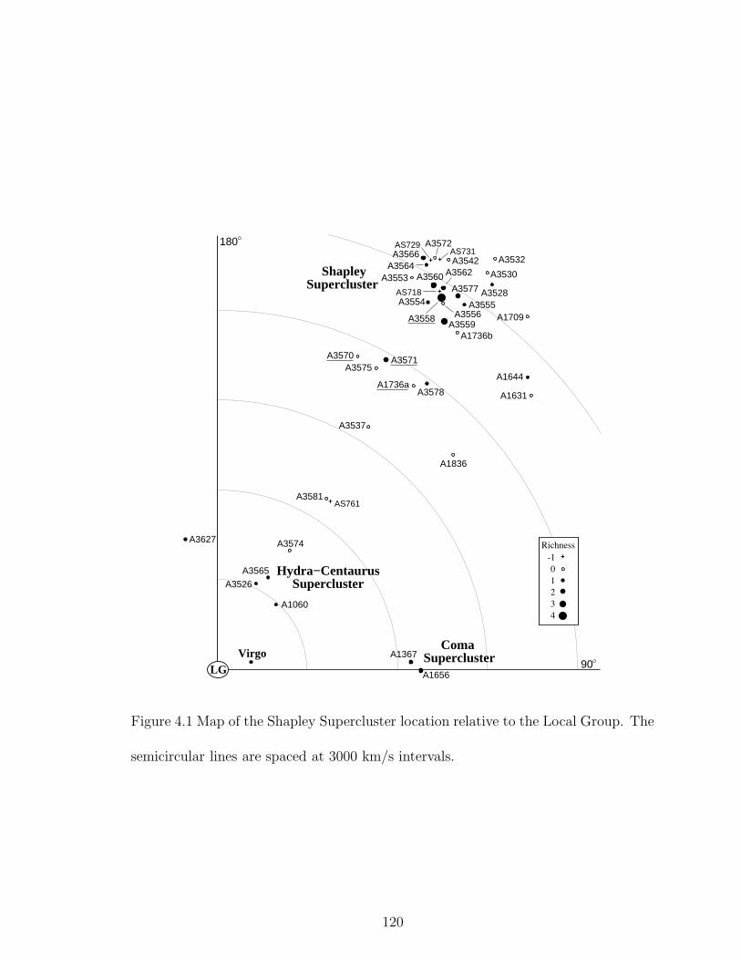
180
90SuperclusterComa
Supercluster Shapley
SuperclusterHydra−Centaurus
-101234
+
Richness
A1736a
Virgo
A1656
A1367
A3526
A3565
A3574
+
+ +
A3555
A3577
A3530
A3554
A3532A3564A3566
A1709
AS718
AS729 A3572
A3542A3562
A3556A3559
A1736b
AS731
A3528
A3571A3570
A3537
A1836
A1644
A1631
A3627
A3560A3553
A3558
A1060
A3575
+ AS761A3581
A3578
LG
Figure 4.1 Map of the Shapley Supercluster location relative to the Local Group. The
semicircular lines are spaced at 3000 km/s intervals.
120
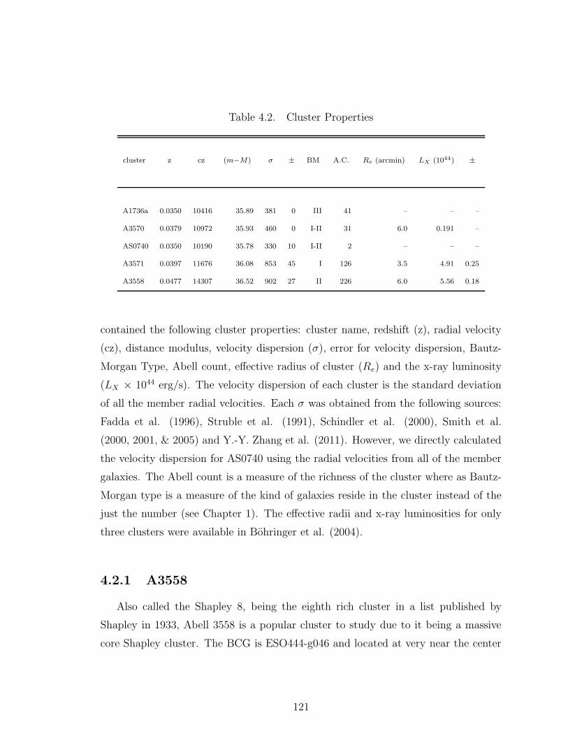
Table 4.2. Cluster Properties
cluster z cz (m−M) σ ± BM A.C. Re (arcmin) LX (1044) ±
A1736a 0.0350 10416 35.89 381 0 III 41 – – –
A3570 0.0379 10972 35.93 460 0 I-II 31 6.0 0.191 –
AS0740 0.0350 10190 35.78 330 10 I-II 2 – – –
A3571 0.0397 11676 36.08 853 45 I 126 3.5 4.91 0.25
A3558 0.0477 14307 36.52 902 27 II 226 6.0 5.56 0.18
contained the following cluster properties: cluster name, redshift (z), radial velocity
(cz), distance modulus, velocity dispersion (σ), error for velocity dispersion, Bautz-
Morgan Type, Abell count, effective radius of cluster (Re) and the x-ray luminosity
(LX × 1044 erg/s). The velocity dispersion of each cluster is the standard deviation
of all the member radial velocities. Each σ was obtained from the following sources:
Fadda et al. (1996), Struble et al. (1991), Schindler et al. (2000), Smith et al.
(2000, 2001, & 2005) and Y.-Y. Zhang et al. (2011). However, we directly calculated
the velocity dispersion for AS0740 using the radial velocities from all of the member
galaxies. The Abell count is a measure of the richness of the cluster where as Bautz-
Morgan type is a measure of the kind of galaxies reside in the cluster instead of the
just the number (see Chapter 1). The effective radii and x-ray luminosities for only
three clusters were available in Bohringer et al. (2004).
4.2.1 A3558
Also called the Shapley 8, being the eighth rich cluster in a list published by
Shapley in 1933, Abell 3558 is a popular cluster to study due to it being a massive
core Shapley cluster. The BCG is ESO444-g046 and located at very near the center
121
of the cluster.
4.2.2 A3570
Abell 3570 is a poor cluster whose BCG is ESO325-g016.
4.2.3 A3571
Abell 3571 is a cluster dominated by a massive elliptical, the BCG, ESO383-g076.
The BCG is located very near the x-ray center of A3570.
4.2.4 A1736a
Abell 1736 is at a redshift of 0.0350, which can be read in Table 4.2, however, there
is confusion in labeling this cluster. There is another cluster named A1736b which is
at a redshift of 0.0458. In some papers the cluster at redshift 0.0350 is called A1736b
and the other is called A1736a or just A1736. Therefore, one is never quite sure which
cluster the study is referring to until the redshift is listed. This cluster is fairly poor
and not dominated by any single massive galaxy. The BCG is ESO509-g008.
4.2.5 AS0740
This cluster contains the nearest known lensing galaxy with Chapter 3 of this
thesis discussing a search for Ultra Compact Dwarfs (UCDs). AS0740 is a poor
cluster with ESO325-g004 as the BCG. The richness of the cluster is the reason it
exists in the Abell supplementary list published by Abell, Corwin and Olowin in 1989.
AS0740 did not meet the original richness criteria. The BCG is also at the cluster’s
X-ray center (Smith 2011) and can be viewed in Figure 4.2, which is a X-ray contour
map of AS0740.
122

Figure 4.2 X-ray map of AS0740, courtesy R. Smith
123

4.3 Data Analysis
4.3.1 ACS/WFC
The Advanced Camera for Surveys (ACS) was installed on the HST in March
2002. ACS has three channels, the High Resolution Channel, the Wide Field Channel
(WFC) and the Solar Blind Channel (SBF). One of the two photometric channels,
WFC, was used to image the 11 galaxies in this study. The resolution is 20 pix/arcsec
with a field of 202 arcsec × 202 arcsec. The image scale for this survey was 33.4 pc/pix
- 43.4 pc/pix. ACS went offline a few times and currently has only two channels in
operation, WFC and SBC (Ford 2003; ACS/HST updates).
4.3.2 Observations
The various galaxies were imaged with ACS/WFC in F814W during 114 orbits,
with the exception of ESO325-g004, which was imaged in the additional filters F475W
and F625W. As previously stated, the HST GO Program 10429 was designed to col-
lect data on the following galaxies to calculate SBF distances: ESO509-g008, ESO509-
g020, ESO509-g067, ESO444-g046, 2mj13275493, 2mj13272961, 2mj13280261, ESO383-
g076, 2mj13481399, ESO325-g016, and ESO325-g004. The exposure times of these
images were 18567s, 18567s, 18567s, 34210s, 35550s, 35550s, 35550s, 21081s, 21081s,
18882s and 18882s, respectively. These more precise distances would give us a better
understanding of the supercluster’s significance to the Local Group’s relative mo-
tion to the CMB. These images were processed with the Apsis pipeline detailed in
Blakeslee et al. (2003). This pipeline is used to sum the exposures, geometrically
correct orientation, and remove cosmic rays from the images. Mosaics of the images
produced can be found in Figure 4.3 and Figure 4.4.
124
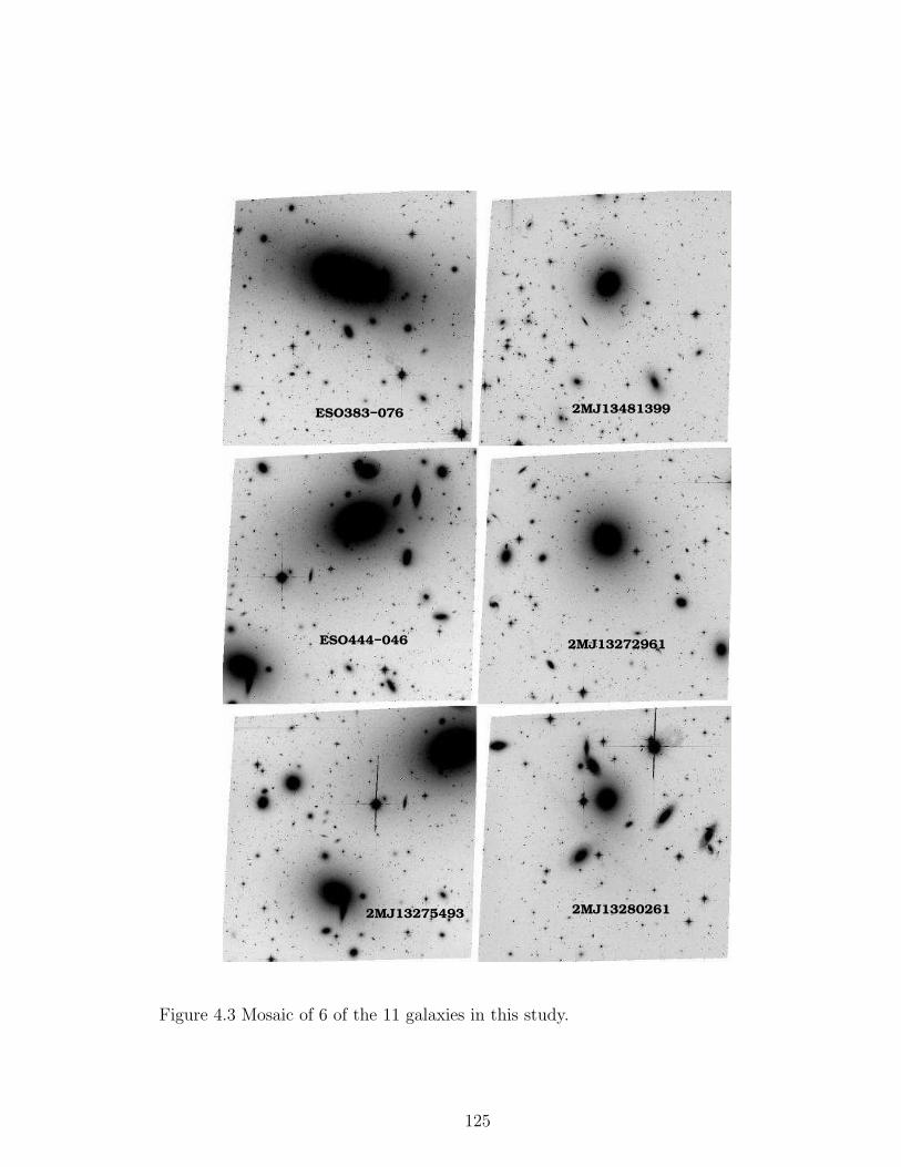
ESO383−076
2MJ13272961ESO444−046
2MJ13481399
2MJ13275493 2MJ13280261
Figure 4.3 Mosaic of 6 of the 11 galaxies in this study.
125
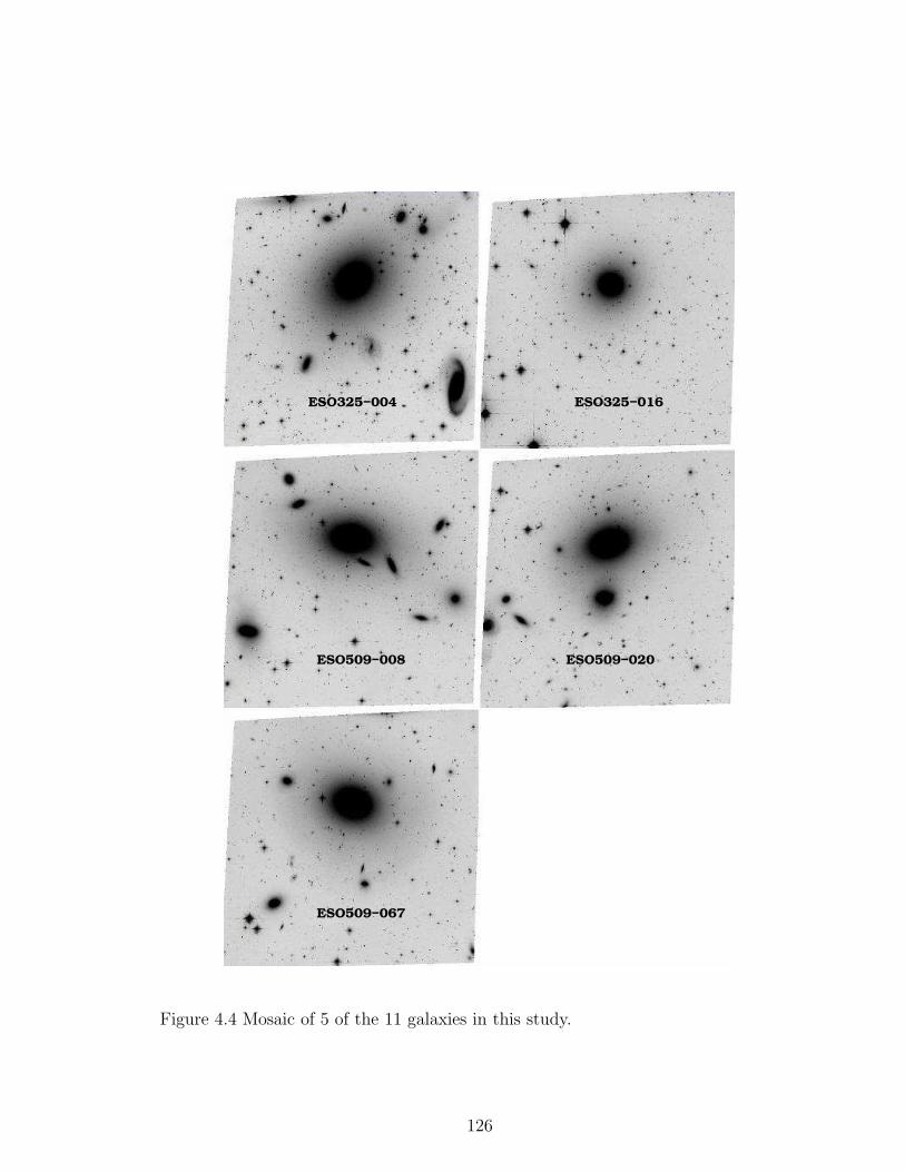
ESO325−004
ESO509−067
ESO509−008 ESO509−020
ESO325−016
Figure 4.4 Mosaic of 5 of the 11 galaxies in this study.
126

4.3.3 Reductions in IRAF/DAOphot
The object detection process for the 11 galaxies was done primarily with IRAF /
DAOphot and is detailed below.
DAOphot (Stetson 1987) is an object detection software program used to perform
stellar photometry, measuring flux or intensity, in crowded fields. This software pack-
age was used within IRAF, which stands for Image Reduction and Analysis Facility.
IRAF is a software system that contains tools for a large amount of astronomical
data reduction (some examples include optical imaging and spectra). The process
that leads to the final catalog of GC candidates was a lengthy one with many steps.
The tasks or algorithms used are in the DAOphot package in IRAF. The first step
was to set all the parameters before any task is done. This object detection software
looks for star-like objects or point sources and at this distance all the GCs are points.
The first task is called daofind and is an algorithm that detects sources and pro-
duces a list of stars from the input image. Figures 4.3 and 4.4 show the 11 galaxy
input images. Daofind searches for point sources within the image that meet the pa-
rameters the user assigns, such as, fwhmpsf, sigma, threshold, datamin, and datamax.
The image is then convolved with a fitted Gaussian and the resulting maxima (from
the parameters) are the objects detected. Daofind computes centers, estimated mag-
nitudes, sharpness and roundness for the selected stars. Sharpness is defined as the
ratio of the amplitude of the best fitting delta function at the position of a detected
object to the amplitude of the best fitting Gaussian at the same position (Stetson
1987). Roundness is computed by fitting a one-dimensional Gaussian function of full
width at half-maximum fwhmpsf to the x and y marginal pixel distributions (Stetson
1987). The output file of the daofind task is called image.coo, where image is replaced
by whatever name belongs to the input image. The image used in this task was the
rescaled image of the galaxy. The rescaled image was the original image divided by
its exposure time and then multiplying by 2680 so that the parameters in datapars,
daopars, and findpars (parameter files) are uniform.
The second task is phot and is run on the same rescaled image. This algorithm
computes initial magnitudes, centers, and sky values from the list compiled by daofind.
127

The values in the star list phot creates are used as starting values for the next steps
in the DAOphot process. Phot first reads in the image.coo file and computes sky
values by looking at fluctuations in the sky background within a defined annulus of
pixels. It then computes an instrumental magnitude and error using the aperture
radii specified in the parameter files. The phot output file is called image.mag.
Next, the pstselect task creates a list of bright, isolated objects as good star
candidates to create a point spread function (psf) model, used in the following task,
psf. The pstselect algorithm reads in an image file and the image.mag file. It first
sorts the stars in the list by magnitude, with the brightest stars at the top of the
list. It then selects the maxnpsf number of brightest stars. In this case we defined
maxnpsf = 100 in the parameter files. Pstselect makes sure none of these stars are
saturated, have any bad pixels and have no close, bright neighbors. The output file
is named image.pst and contained a list of bright stars their id, x and y coordinates,
magnitudes and sky values of the selected stars.
Once the list of 100 objects is selected, we interactively look at each object using
the psf task to see if it can contribute to a psf model. This psf model will be used
by the allstar to compute magnitudes using psf fitting instead of apertures like in
phot. The psf algorithm uses image.pst. and displays the contour, radial, and 3D
mesh plot of each star in the list. From these plots one chooses which of the stars in
the list will be accepted. Doing this task interactively is essential to the fitting since
a significant number of the stars in the 100 star list turn out not to be point sources.
Once all the stars in the list have either been accepted or rejected, the remaining
stars are compiled and are fitted to a analytic function. Since auto was chosen in the
parameter file, the following functions are tried until one fits best: gauss, moffat25,
128

moffat15, penny1, penny2, and lorentz.
z =x2
p12+
y2
p22
gauss = A ∗ exp(−0.5z)
z =x2
p12+
y2
p22+ xyp3
moffat15 =A
(1 + z)1.5
moffat25 =A
(1 + z)2.5
z =x2
p12+
y2
p22+ xyp3
lorentz =A
1.0 + z
z =x2
p12+
y2
p22
e =x2
p12+
y2
p22+ xyp4
penny1 =A ∗ (1 − p3)
1.0 + z+ p3 ∗ exp(−0.693 ∗ e)
z =x2
p12+
y2
p22+ xyp5
e =x2
p12+
y2
p22+ xyp4
penny2 =A ∗ (1 − p3)
1.0 + z+ p3 ∗ exp(−0.693 ∗ e) (4.1)
The psf model can vary with respect to its position in the image. This is controlled
by the parameter varorder. We used varorder of 2, which modeled a psf that varies
quadratically with position. Psf produces a list of the stars, another image.pst file, a
list of grouped stars (on the basis of position and signal-to-noise), image.psg, and an
image of the created psf model.
Once a psf model is made, the allstar task is run. This task fits the psf model to
each object it finds in the image and assigns a magnitude and error to that object and
to the sky. It also calculates a χ and sharpness value. The definition of sharpness is
a measure of the difference between the observed width of the object and the width
of the psf model (Stetson 1987). The definition of χ is the ratio of the observed
129

pixel-to-pixel scatter in the fit residuals to the expected scatter calculated from a
predictive model based on measured detector features (Sabbi et al. 2008). Allstar
produces a subtracted image where all the objects the program found are removed
from the original image.
This first sequence of tasks is done to make an image to use in the median process.
This process is designed to create a smoothed image from the subtracted image. This
will smooth the edges of the areas where the objects were removed. This leaves an
image that is mostly devoid of all unresolved objects. Once this smoothed image
is subtracted from the original image most of the large objects will be masked or
erased. Now we have something we call a flat image (which is like the masked image
mentioned in the NGC1533 chapter on data reduction). This image has all the big
objects removed and now we are free to try to detect objects (our GC candidates)
without the distraction of large foreground stars or background galaxies. Again the
first run’s sole purpose was to get this flat image, which will be used, in the data
detection process.
The sequence of daofind, phot and allstar is run again. The process is exactly like
the first run with the exception of not having to perform pstselect or psf because we
can use the psf model found in the first run. However, even though daofind and phot
are run with the flat image, allstar is run with the original rescale image. The .mag
output file from phot will help allstar avoid all the non-star-like objects in the image
(as mentioned earlier). This time we are running it to actually catalog our objects.
Using our flat image we get a .mag file and an .als file. We use the subtracted image
from this allstar process for our last and final run. When this .sub.fits image is
subtracted from the flat image, we get an image that only has the objects missed in
the object detection in this run (we call it sub.flat.fits). This final run is to detect
and get photometry for any missed star-like objects. Daofind and phot are run with
the sub.flat.fits. The .mag files from run 2 and run 3 are combined and then given to
allstar for this final run. This combined .mag file has all the objects found in round
2 and then in round 3 (where we are trying to find any candidates that were missed
in round 2). The .als file (called 3.als) of this last run of allstar is our final catalog
of candidates. The task pdump is used to create a more condensed and cleaned up
130

final list. It consists of id, xc, yc, mag, magerr, sharp and chi (χ). We called this
final catalog 3.dat. Once we have this photometry file we do a similar process to get
completeness.
4.3.4 Magnitude Correction
The magnitudes need to be corrected for extinction and aperture effects for the
ACS camera as in Sirianni et al. (2005), as well as for the DAOphot fitting aperture.
Extinction & Photometric Corrections
Galactic Extinction is the effect that causes the magnitude of a stellar object
to dim due to photons being scattered and absorbed by the dust in the interstellar
medium. The parameter A is called the galactic extinction and is defined as the
difference between the magnitude that is observed, m, and the magnitude that would
be observed in the absence of dust, mo and can be written in the following equation,
AX = (m − mo)X (4.2)
where X is the X-band, the filter in which the magnitude is measured.
If extinction is known in two filters then a value defined as the difference is called
reddening or color excess E(X-Y) and is described in the following equation,
E(X − Y ) = [m(X) − m(Y )] − [mo(X) − mo(y)] = AX − AY (4.3)
where X is the X-band and Y is the Y-band (Binney 1998).
The E(B-V) are available in NED based on the dust maps of Schlegel et al. (1998)
for each galaxy and are listed in Table 4.3 at the end of this section. These values
needed to be converted to AI since our images were taken in the F814W bandpass
and therefore give magnitudes in the I-band. This conversion is done using data from
Siranni et al. 2004. They give a value of 1.8 for the F814W filter and early-type
galaxy. Thus, AI can be obtained for each galaxy the following way:
E(X − Y ) ∗ 1.8 = AI (4.4)
131

There is also an aperture correction of -0.09 for an aperture of r = 5pix (0.25
arcsec) using ACS in the F814W filter (Sirianni 2005).
Aperture correction within DAOphot
Since all of the magnitudes are coming from psf fitting of objects during the allstar
task, we need to calculate what aperture correction must to be applied in order to
obtain total magnitudes. We do this by making a list omitting the brightest 1000
stars in the final allstar catalog. This list is used in the task substar, which produces
an image that subtracts all objects in the list, leaving only the 1000 brightest stars.
The phot task is run on this image using an aperture of 10 pixels in diameter (which
corresponds to an aperture of 0.5 arcsec). Comparing the .mag file that phot produces
to the image3.dat file from the final allstar run will give the difference between the
psf fitted magnitudes and the aperture 10pix magnitudes. The following Figures 4.5-
4.7, show plots of the difference in magnitude values (aperture magnitude from the
brightest stars minus allstar magnitude verses the allstar magnitude. The correlation
shown in Figures 4.5- 4.7 give the aperture correction that needs to be applied to each
magnitude value. The median difference is labeled in each plot next to the galaxy
name.
Table 4.3 contains the aperture correction (Sirriani aperture correction plus DAOphot
aperture correction from previous plots) in the first column, with the second column
listing the E(B-V) values from NED. The third column in the extinction values in the
I-band. The last column is the total correction, apercor + AI .
4.3.5 Completeness
By adding a known number of artificial stars (with given magnitudes) to the im-
age and then running the same detection and measurement process, one can see the
fraction of objects the software does not detect. The percentage of objects detected
as a function of magnitude is called completeness function. The completeness pro-
gressively decreases as you get to fainter and fainter objects (higher magnitudes, see
132
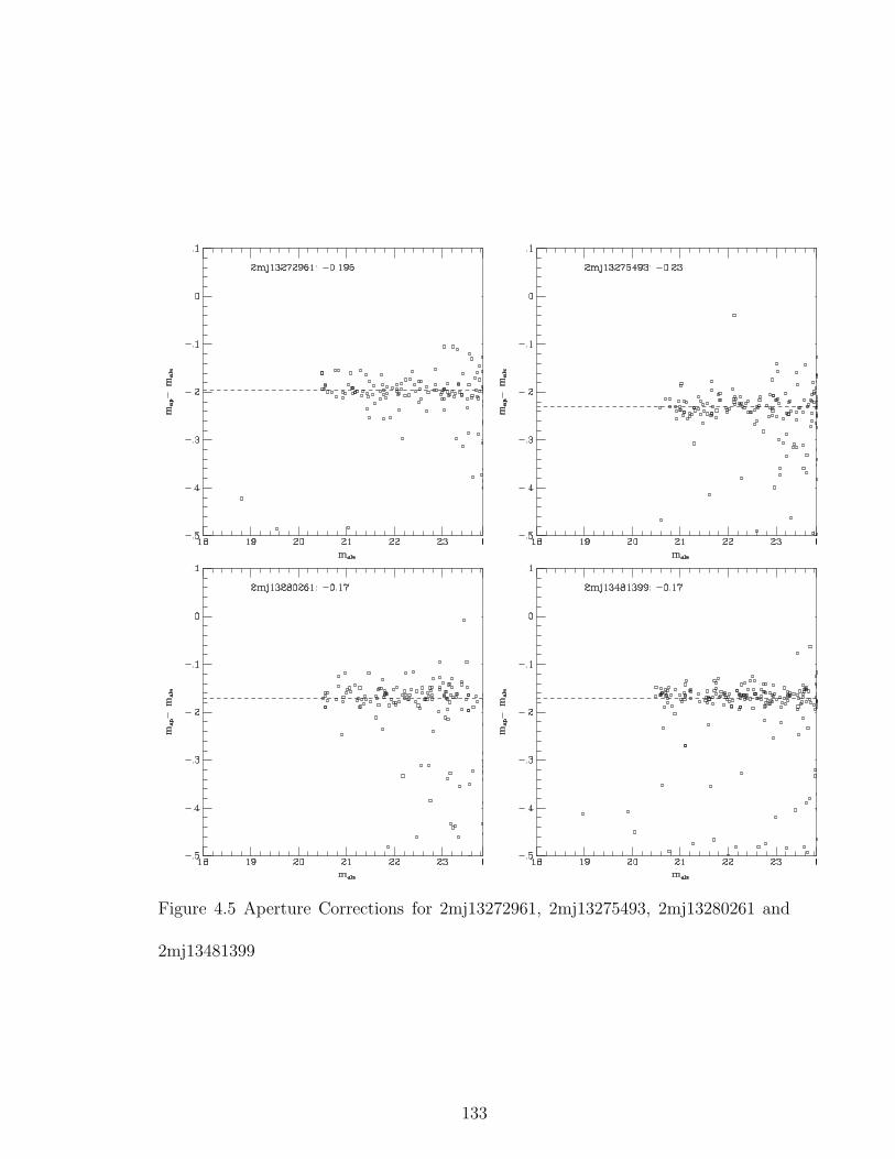
Figure 4.5 Aperture Corrections for 2mj13272961, 2mj13275493, 2mj13280261 and
2mj13481399
133
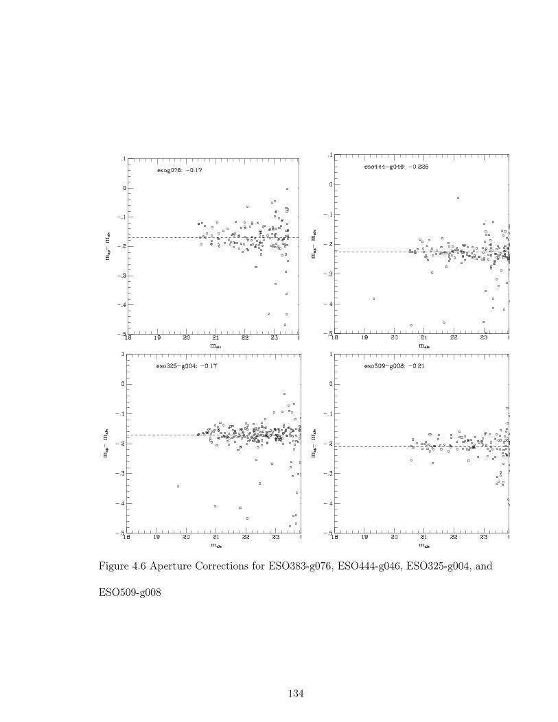
Figure 4.6 Aperture Corrections for ESO383-g076, ESO444-g046, ESO325-g004, and
ESO509-g008
134

Figure 4.7 Aperture Corrections for ESO325-g016, ESO509-g020, and ESO509-g067
135
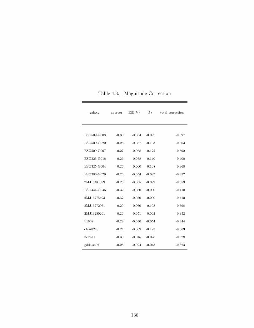
Table 4.3. Magnitude Correction
galaxy apercor E(B-V) AI total correction
ESO509-G008 -0.30 -0.054 -0.097 -0.397
ESO509-G020 -0.28 -0.057 -0.103 -0.363
ESO509-G067 -0.27 -0.068 -0.122 -0.392
ESO325-G016 -0.26 -0.078 -0.140 -0.400
ESO325-G004 -0.26 -0.060 -0.108 -0.368
ESO383-G076 -0.26 -0.054 -0.097 -0.357
2MJ13481399 -0.26 -0.055 -0.099 -0.359
ESO444-G046 -0.32 -0.050 -0.090 -0.410
2MJ13275493 -0.32 -0.050 -0.090 -0.410
2MJ13272961 -0.29 -0.060 -0.108 -0.398
2MJ13280261 -0.26 -0.051 -0.092 -0.352
b1608 -0.29 -0.030 -0.054 -0.344
class0218 -0.24 -0.069 -0.123 -0.363
field-14 -0.30 -0.015 -0.028 -0.328
gdds-sa02 -0.28 -0.024 -0.043 -0.323
136

Chapter 1).
The task in DAOphot used to add additional artificial stars is called addstar.
Addstar also produces a list of the magnitudes and positions of the added artificial
stars. This file is called an image.art file. We do two runs of daofind, phot and allstar
to get a final catalog of objects detected. We only do two runs instead of the three,
which is explained in the previous section. The first run was just done to get the
flat image, which we then use here for the final two runs. The final catalog is called
add3.dat (created by using pdump on the final allstar file). Once we have the add3.dat
files we can compare this final list to the list of stars added to the image. We can
now see the number of added objects actually detected.
This information was binned by magnitude. The bins range from magnitude 20 to
29 by increments of 0.5. The image.art file and the add3.dat file are binned individu-
ally by magnitude. Then we can make a file where each bin will have number detected
divided by the number inserted into the image. This file is called completeness.bin
and used in a python script called pritchfit.py to obtain essential parameters, α and
m0 (the magnitude when completeness reaches 50 percent; not to be confused with
the m0 in the extinction section) for a completeness curve that follows this equation:
f = 0.5(α(m − m0)
2√
[1 + α2(m − m0)]) (4.5)
The output for pritchfit.py is an α and mO and a file with a list of values for
the completeness with errors. Once these values are plotted with the data from
the completeness.bin file, we obtain the completeness curves. These curves are the
presented in following Figures 4.8- 4.10, showing f verses magnitude.
The values obtained to create these plots are listed in Table 4.4 where the columns
match the parameters in equation 4.5.
4.3.6 Background
At this distance, our GC candidates are point sources therefore to make sure
we are not counting foreground stars or background galaxies, we use ”background”
137

Figure 4.8 Completeness Curves for 2mj13275493, 2mj13481399 (top row),2mj13272961, and 2mj13280261 (bottom row) plotted with percentage of detectedobjects versus magnitude.
138
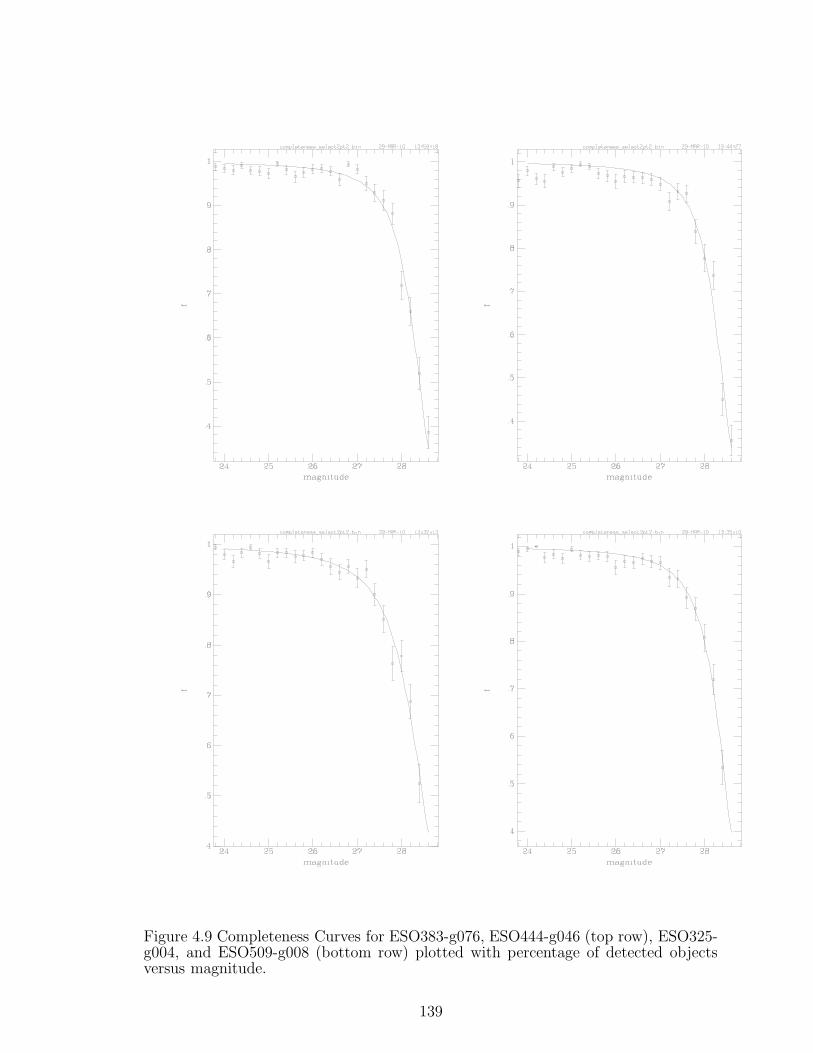
Figure 4.9 Completeness Curves for ESO383-g076, ESO444-g046 (top row), ESO325-g004, and ESO509-g008 (bottom row) plotted with percentage of detected objectsversus magnitude.
139
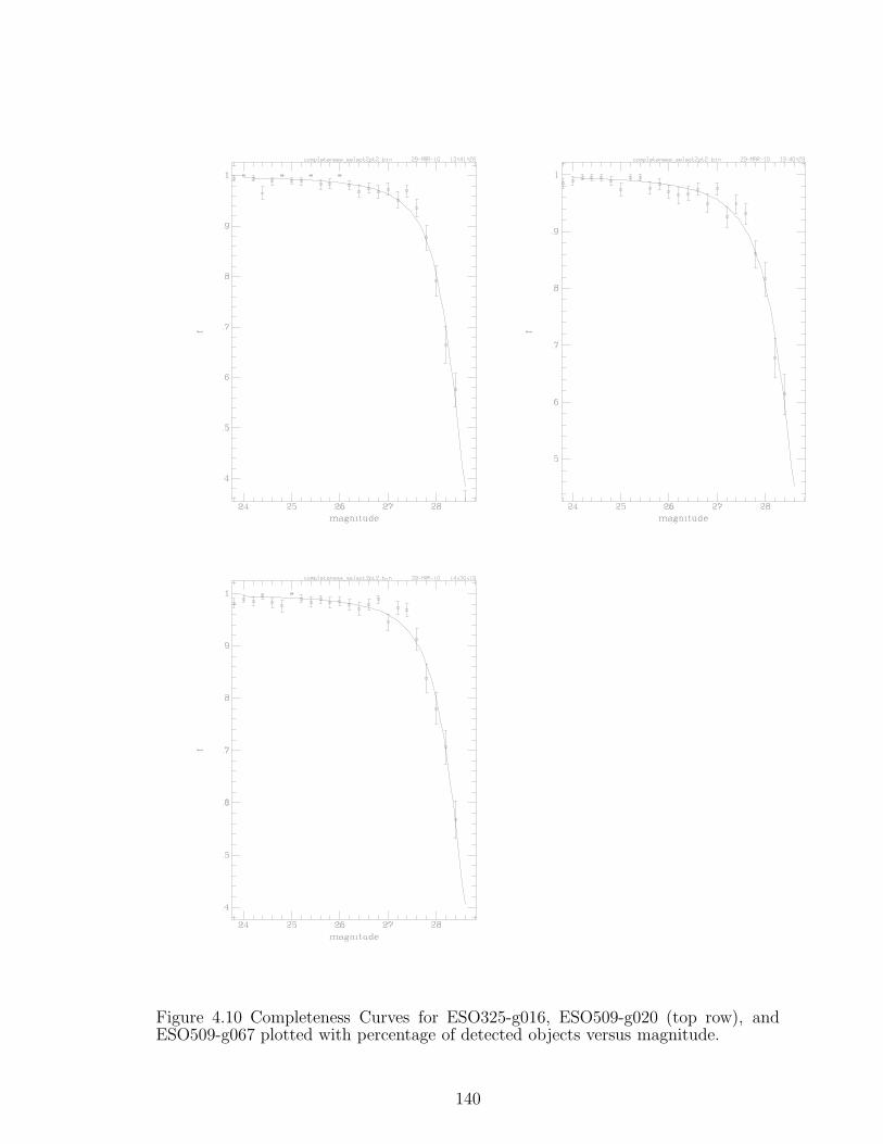
Figure 4.10 Completeness Curves for ESO325-g016, ESO509-g020 (top row), andESO509-g067 plotted with percentage of detected objects versus magnitude.
140
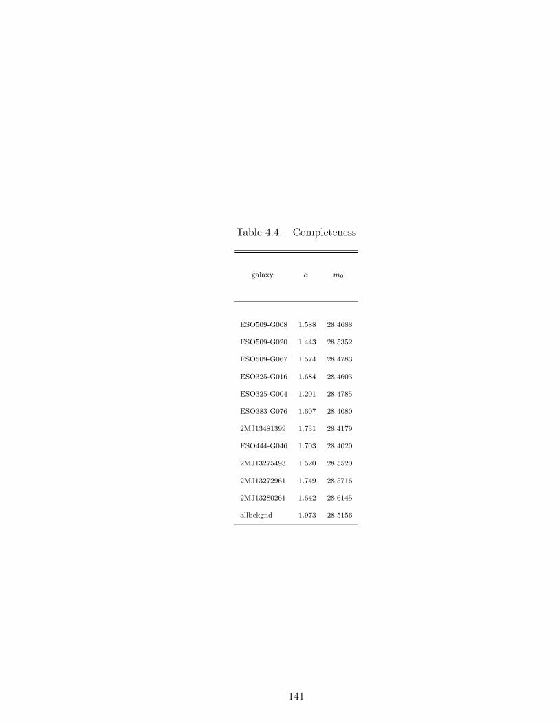
Table 4.4. Completeness
galaxy α m0
ESO509-G008 1.588 28.4688
ESO509-G020 1.443 28.5352
ESO509-G067 1.574 28.4783
ESO325-G016 1.684 28.4603
ESO325-G004 1.201 28.4785
ESO383-G076 1.607 28.4080
2MJ13481399 1.731 28.4179
ESO444-G046 1.703 28.4020
2MJ13275493 1.520 28.5520
2MJ13272961 1.749 28.5716
2MJ13280261 1.642 28.6145
allbckgnd 1.973 28.5156
141

fields with similar galactic latitudes taken through the same F814W filter. We run
the ”background” fields though the same data analysis (DAOphot and selection and
listed in Table 4.3 for magnitude correction) and then subtract just the number
of objects detected in that magnitude range from the GC candidates detected to
get a background corrected number of objects. The following Figure 4.11 is that
of each field’s histogram of N galaxies verses I band magnitude. The dotted line
represents ∼ 28.5 as our initial faint magnitude cutoff. This choice is supported by
the completeness curves in 4.8-4.10 that show the magnitude in which completeness
falls to 50% at around 28.5 for each galaxy.
4.3.7 Selection
Sharpness and χ
To better narrow down the lists of objects obtained from DAOphot, we chose
to cut the data files with respect to two parameters, χ and sharpness from the final
allstar output file image3.als (defined in section 4.3.3). Since we only have data in one
filter for all but one galaxy, size and color cannot be used to help discern which objects
are good GC candidates in our list of detected objects. Once χ and sharpness were
plotted against magnitude and each other, correlations were found. Figures 4.12-
4.15 show these correlations for 4 different galaxies. The plots of the top row are
the values obtained without masking out the uneven edges of each image. Since
the galaxy images are summed from several dithered exposures the edges can be very
noisy. Noise can cause many false detections at the edges of the image. Once they are
masked stronger correlations can be seen (bottom row of Figures 4.12- 4.15). These
plots also show that the fainter the magnitude, the more non-point sources detected.
DAOphot’s manual suggests the values for χ and sharpness are good indicators of
whether a detected object is a point source (star) or not. χ should be ∼ 1 or it is not
a star. This is why the range of χ < 2 was chosen. It also suggests that stars should
have a sharpness value of ∼ 0, and deviates greatly from 0 if they are cosmic rays
or other bad pixels in the image. Beaulieu et al. (2001) used a sharpness range of
142
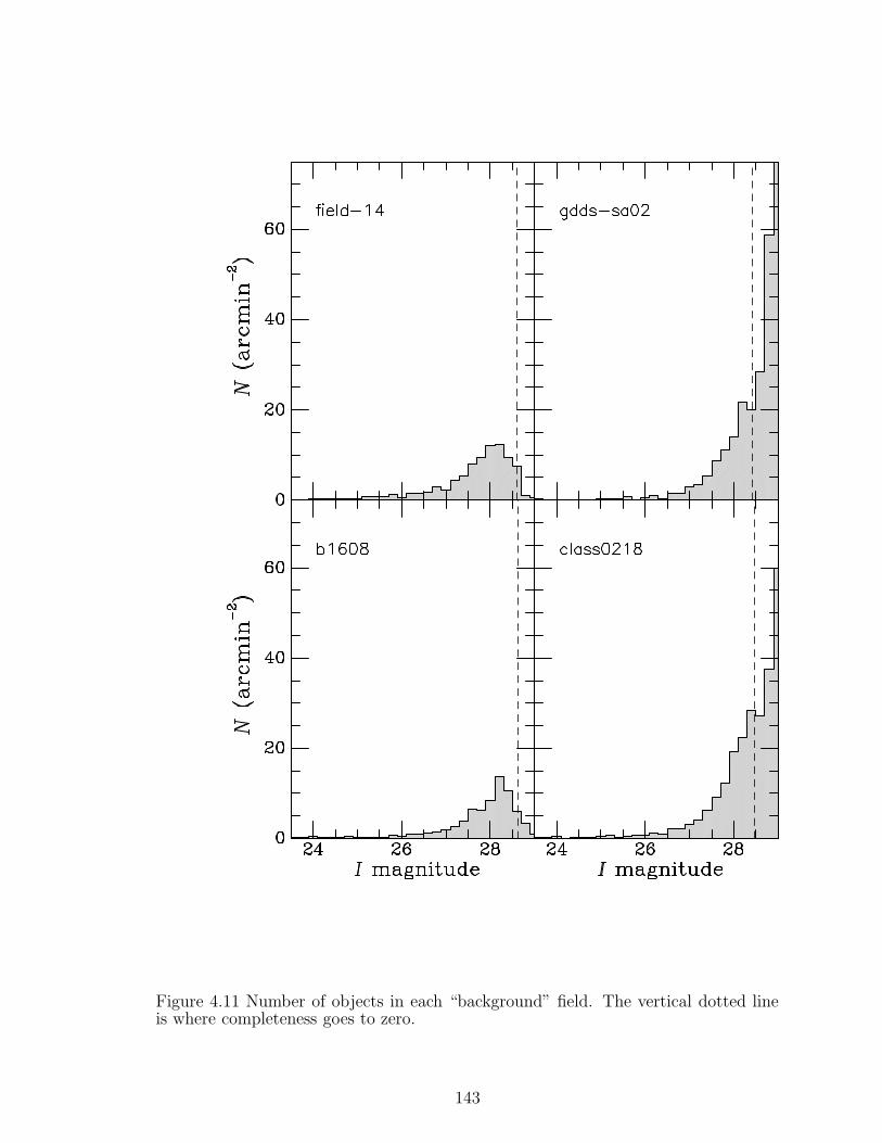
Figure 4.11 Number of objects in each “background” field. The vertical dotted lineis where completeness goes to zero.
143

-0.2 to 3.0, which seemed reasonable compared to our own plots. Sabbi et al. (2008)
chose χ < 4 and a range of -.5 < sharpness < .5 for the F814w filter. Looking at the
histograms of sharpness verses magnitude, Figures 4.16- 4.18, the scatter around zero
is from -0.2 to 3.0 with some plots showing another bump at 0.5. We decided on the
selection range of sharpness -0.2 to 3.0 for our GC candidates.
Magnitude
A magnitude cut of 23.5 to 27.5 was applied to select GC candidates. The faint
cut is 27.5 because past this magnitude we cannot get reasonable completeness, the
completeness falling below 90% around 27.5 (see Figures 4.8- 4.10). The famous
globular cluster luminosity function, discussed in Chapter 1 and the following section,
shows at these distances GCs will not have magnitudes much brighter than 23.5, which
is the basis for our bright cut.
4.4 GCLF
In Chapter 1 it was explained that the Globular Cluster Luminosity Function
(GCLF) was assumed to be universal for globular cluster systems. Our data does not
go far enough beyond the turnover (peak of Gaussian luminosity function) to give a
reliable fit. Therefore, our data cannot be used for distance measurements. However,
it is interesting to plot the GCLF that is available and see if an extrapolated turnover
corresponds to the known distances to these Abell clusters.
Using distance moduli for each cluster from NED and MI = -8.5 mag (Harris et
al. 2009), a value for the turnover magnitudes, m0 from equation 1.6, was calculated
for each cluster: A3558 = 28.02, A3570 = 27.43, A3571= 27.58, A1736a = 27.39, and
AS0740 = 27.28. In Figures 4.19- 4.21) show the “background” population in red and
the detected GCs in black. These histograms match the first half of the Gaussian
curve and when the background is taken into account, the turnover magnitudes seem
to match the values obtained from NED.
144
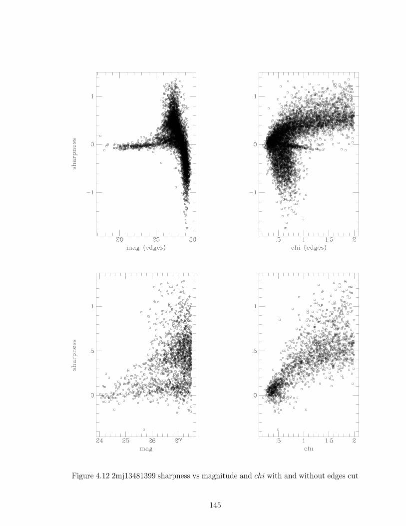
Figure 4.12 2mj13481399 sharpness vs magnitude and chi with and without edges cut
145

Figure 4.13 2mj13272961 sharpness vs magnitude and chi with and without edges cut
146

Figure 4.14 eso509-g008 sharpness vs magnitude and chi with and without edges cut
147
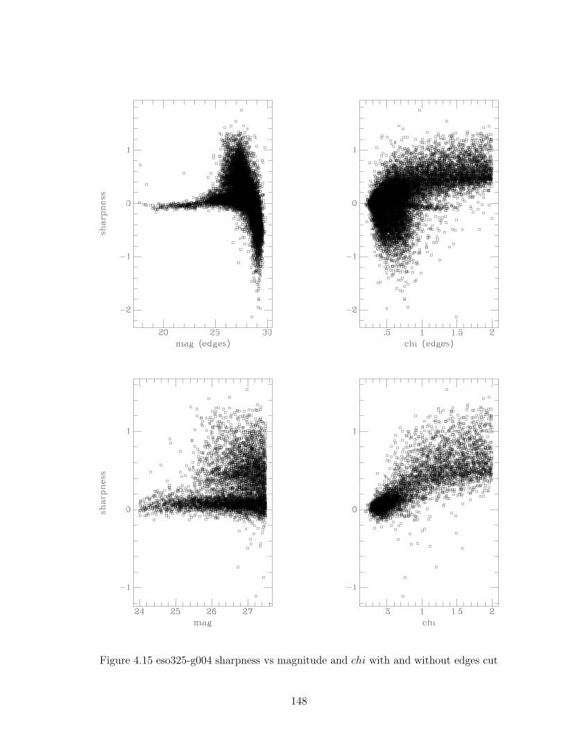
Figure 4.15 eso325-g004 sharpness vs magnitude and chi with and without edges cut
148
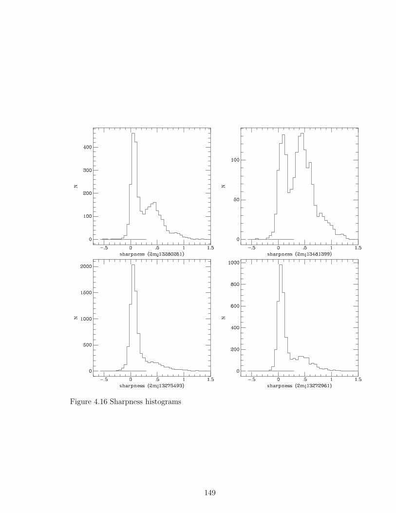
Figure 4.16 Sharpness histograms
149

Figure 4.17 Sharpness histograms
150
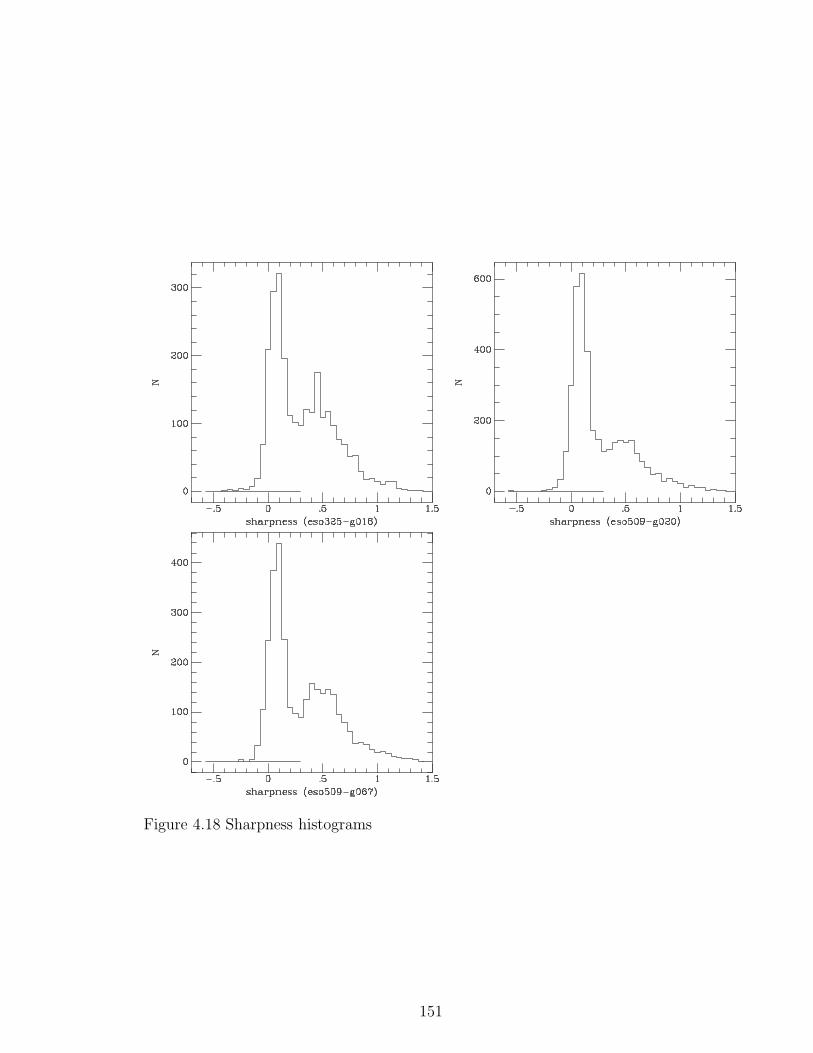
Figure 4.18 Sharpness histograms
151
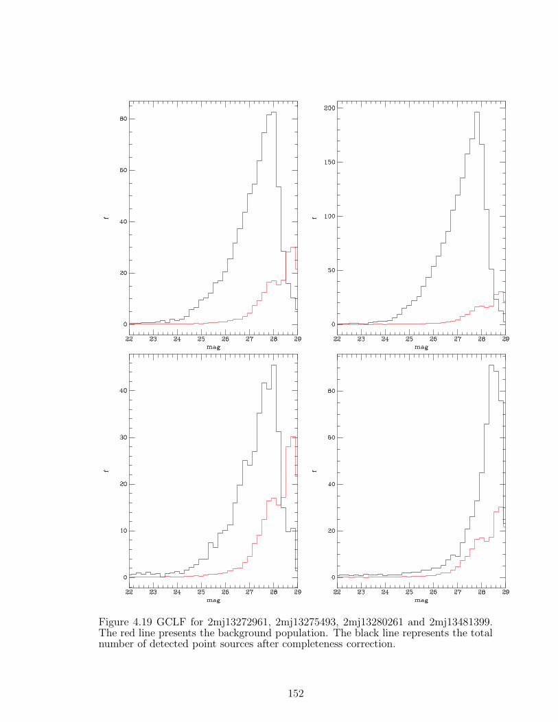
Figure 4.19 GCLF for 2mj13272961, 2mj13275493, 2mj13280261 and 2mj13481399.The red line presents the background population. The black line represents the totalnumber of detected point sources after completeness correction.
152

Figure 4.20 GCLF for ESO383-g076, ESO444-g046, ESO325-g004, and ESO509-g008.The red line presents the background population. The black line represents the totalnumber of detected point sources after completeness correction.
153
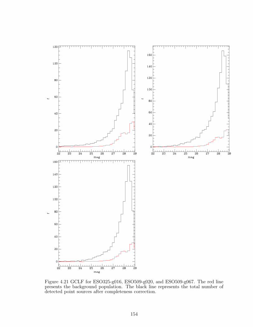
Figure 4.21 GCLF for ESO325-g016, ESO509-g020, and ESO509-g067. The red linepresents the background population. The black line represents the total number ofdetected point sources after completeness correction.
154
Bibliography
[1] Beaulieu, S. F., Gilmore, G., Elson, R. A. W., Johnson, R. A., Santiago, B.,
Sigurdsson, S., & Tanvir, N. 2001, AJ, 121, 2618
[7] Binney, J., & Merrifield, M. 1998, Galactic astronomy / James Binney and Michael
Merrifield. Princeton, NJ : Princeton University Press, 1998. (Princeton series in
astrophysics) QB857 .B522 1998
[3] Blakeslee, J. 2004, HST Proposal, 10429
[4] Blakeslee, J. P., Anderson, K. R., Meurer, G. R., Benıtez, N., & Magee, D. 2003,
Astronomical Data Analysis Software and Systems XII, 295, 257
[4] Bohringer, H., et al. 2004, A&A, 425, 367
[6] Fadda, D., Girardi, M., Giuricin, G., Mardirossian, F., & Mezzetti, M. 1996, ApJ,
473, 670
[7] Ford, H. C., et al. 2003, Proc. SPIE, 4854, 81
[8] Harris, W. E. 2009, ApJ, 703, 939
[9] Lynden-Bell, D., Faber, S. M., Burstein, D., Davies, R. L., Dressler, A., Terlevich,
R. J., & Wegner, G. 1988, ApJ, 326, 19
[10] Postman, M., & Lauer, T. R. 1995, ApJ, 440, 28
[11] Sabbi, E., Gallagher, J. S., Smith, L. J., de Mello, D. F., & Mountain, M. 2008,
ApJ, 676, L113
155
[12] Schindler, S. 2000, A&AS, 142, 433
[13] Schlegel, D. J., Finkbeiner, D. P., & Davis, M. 1998, ApJ, 500, 525
[14] Shapley, H. 1930, Harvard College Observatory Bulletin, 874, 9
[15] Smith, R. J., Lucey, J. R., Hudson, M. J., Schlegel, D. J., & Davies, R. L. 2000,
MNRAS, 313, 469
[16] Smith, R. J., Lucey, J. R., Schlegel, D. J., Hudson, M. J., Baggley, G., & Davies,
R. L. 2001, MNRAS, 327, 249
[17] Smith, R. J., Blakeslee, J. P., Lucey, J. R., & Tonry, J. 2005, ApJ, 625, L103
[18] Stetson, P. B. 1987, PASP, 99, 191
[19] Struble, M. F., & Rood, H. J. 1991, ApJS, 77, 363
[20] van den Bergh, S. 2000, PASP, 112, 529
[23] Zhang, Y.-Y., Andernach, H., Caretta, C. A., Reiprich, T. H., Bohringer, H.,
Puchwein, E., Sijacki, D., & Girardi, M. 2011, A&A, 526, A105
156
Chapter 5
Shapley Supercluster Results
5.1 Number of Globular Clusters Counted
5.1.1 Completeness and “Background” Correction
To obtain the total population of GCs for each of the 11 galaxies studied, we
must perform the proper corrections. DAOphot detects objects in the image and
using various cuts, described in Chapter 4, a list of detected objects is recorded. The
number of GC candidates in this detected list is then scaled to produce the total
number of GCs associated to the host galaxy corrected for completeness and area.
The completeness procedure is performed due to our detection software missing
a certain number of objects depending on the object’s magnitude. When objects
become too faint they are more difficult to detect, therefore, efficiency in detection
decreases with increasing magnitude. This exercise calculates the percentage of ob-
jects the software is detecting within magnitude bins. We can then use the complete-
ness correction curves to scale the detected objects to total number of GCs in the
image. There are also a number of background objects and foreground objects in
the field, so there needs to be a “background” correction. As discussed in Chapter
157

4, the HST archive was searched for images taken in the same filter, F814W, and at
similar Galactic latitude. We picked four background fields and performed the same
data reduction described in the DATA section (DAOPhot). The background detec-
tion lists were subject to the same selection in χ, sharpness and magnitude as the
catalogs for the 11 Shapley Supercluster galaxies. Once these selections were applied,
the background field catalogs were combined into one file. The “background” object
list was then binned by magnitude, as were the detected objects in the 11 galaxies.
By subtracting the binned background file from the binned galaxy file, we completed
another correction to obtain a value for the total number of GCs. A python script
was created to take into account the correction for completeness, background and
magnitude (luminosity function). The next correction to get total number of GCs
associated with a host galaxy is a consequence of the initial magnitude cut and the
subject of the next section.
5.1.2 Magnitude Range and the GCLF Correction
In Chapter 4, we discuss the selection criteria for GC candidates. One selection
was magnitude cuts due to the inability to detect objects much fainter than the
turnover, which is 27.5 ± 0.5 depending on the Abell cluster distance. Since we are
detecting objects only in a magnitude range of mbright = 23.5 to mfaint = 27.5, we are
limiting our search for GC candidates. The globular luminosity function (see Chap 1
for full description) shows us that magnitudes of a GC population follow a Gaussian
curve with m0 as the peak magnitude and σ equal to the standard deviation. This
shape can be seen in Figure 5.1. The GCs with magnitude above and below our
range, whose existence is suggested by this Gaussian curve, need to be counted in
the total number of GCs. These additional globular clusters are taken into account
by considering a ratio of areas in luminosity space. If we are counting only a fraction
of the total number of GCs, that fraction is equal to the ratio of the corresponding
areas under the Gaussian curve or integral and may be represented in the following
way,
158
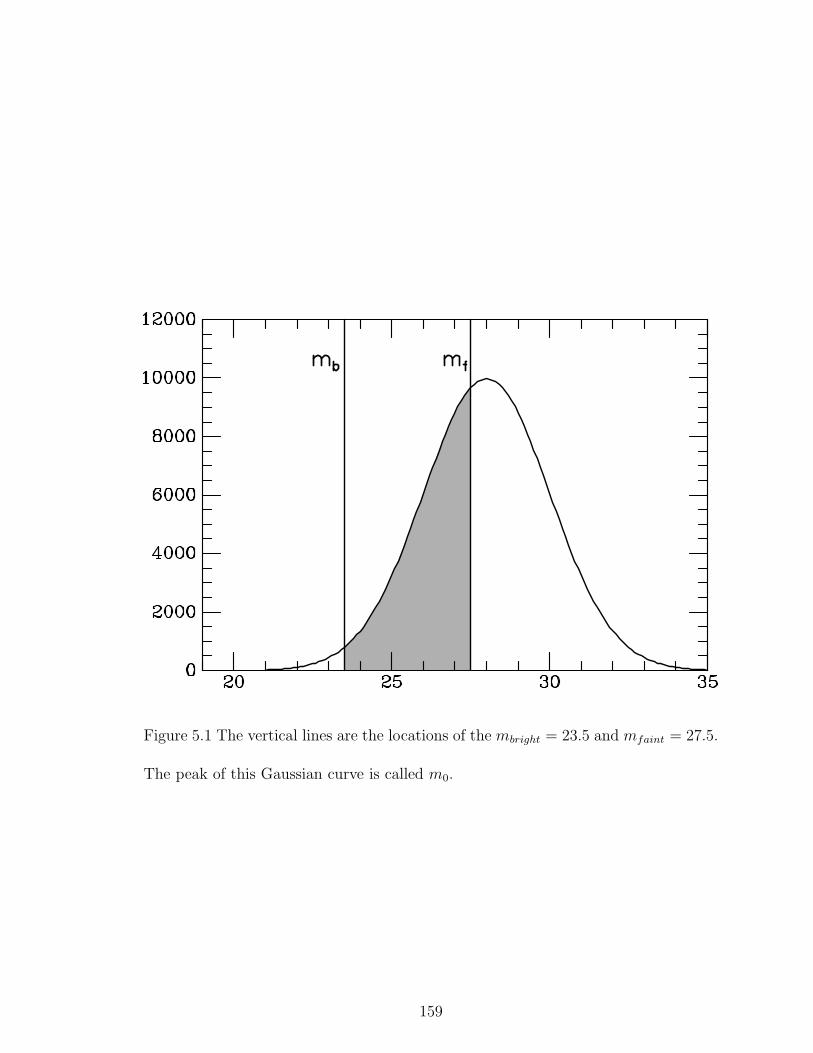
Figure 5.1 The vertical lines are the locations of the mbright = 23.5 and mfaint = 27.5.
The peak of this Gaussian curve is called m0.
159
Ncount
Ntot
= % counted =area under curve between magnitude selection range
total area under Guassian curve(5.1)
where Ncount is the value of the number of GCs associated with the host galaxy
after completeness and background corrections are applied. If we take the total area
under the curve to be one, we can calculate the total number of GCs, Ntot, using the
following equation,
Ncount
Ntot=
1
2[erf(a) − erf(b)] (5.2)
where the 1/2 is from the symmetry of the Gaussian and the erf(x) is the error
function, a fractional integral of a Gaussian over the range -x to x in units of sigma.
Here the values a and b are obtained by the difference in magnitudes divided by
sigma, a =m0−mbright
σand b =
m0−mfaint
σ
5.2 Distribution of GCs and a Radial Correction
The corrections in the previous section were applied to obtain a more realistic
total number of GCs associated with the host galaxy. However, the image does not
display the whole GC population, so there must be a radial correction. There is also
the possibility of the GC population of close neighboring galaxies overlapping.
5.2.1 Distribution of Detected GCs
Here the distribution of the GC candidates, selected from only detection software
output lists, can be seen. In the following plots, Figures 5.2 - 5.7, the GCs detected
are more concentrated toward the center of the host galaxy. The number in each
radial bin is plotted against mean radius of each bin. When the detected objects
are plotted using their x,y coordinates, the GC population follows an approximately
round distribution about the center of the host galaxy (Figures 5.8 - 5.10). However,
160
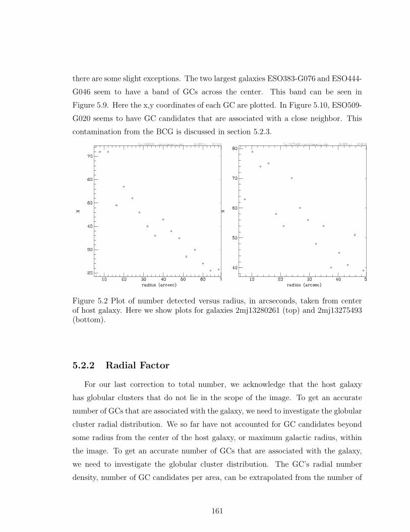
there are some slight exceptions. The two largest galaxies ESO383-G076 and ESO444-
G046 seem to have a band of GCs across the center. This band can be seen in
Figure 5.9. Here the x,y coordinates of each GC are plotted. In Figure 5.10, ESO509-
G020 seems to have GC candidates that are associated with a close neighbor. This
contamination from the BCG is discussed in section 5.2.3.
Figure 5.2 Plot of number detected versus radius, in arcseconds, taken from centerof host galaxy. Here we show plots for galaxies 2mj13280261 (top) and 2mj13275493(bottom).
5.2.2 Radial Factor
For our last correction to total number, we acknowledge that the host galaxy
has globular clusters that do not lie in the scope of the image. To get an accurate
number of GCs that are associated with the galaxy, we need to investigate the globular
cluster radial distribution. We so far have not accounted for GC candidates beyond
some radius from the center of the host galaxy, or maximum galactic radius, within
the image. To get an accurate number of GCs that are associated with the galaxy,
we need to investigate the globular cluster distribution. The GC’s radial number
density, number of GC candidates per area, can be extrapolated from the number of
161
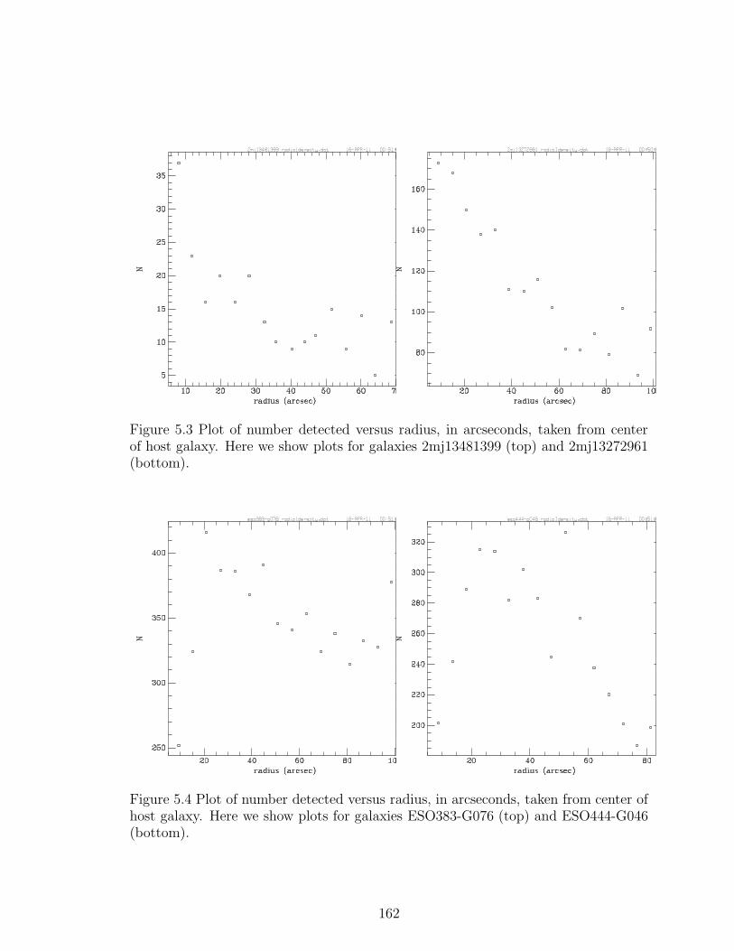
Figure 5.3 Plot of number detected versus radius, in arcseconds, taken from centerof host galaxy. Here we show plots for galaxies 2mj13481399 (top) and 2mj13272961(bottom).
Figure 5.4 Plot of number detected versus radius, in arcseconds, taken from center ofhost galaxy. Here we show plots for galaxies ESO383-G076 (top) and ESO444-G046(bottom).
162
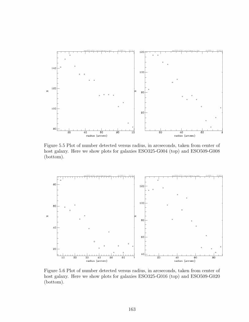
Figure 5.5 Plot of number detected versus radius, in arcseconds, taken from center ofhost galaxy. Here we show plots for galaxies ESO325-G004 (top) and ESO509-G008(bottom).
Figure 5.6 Plot of number detected versus radius, in arcseconds, taken from center ofhost galaxy. Here we show plots for galaxies ESO325-G016 (top) and ESO509-G020(bottom).
163
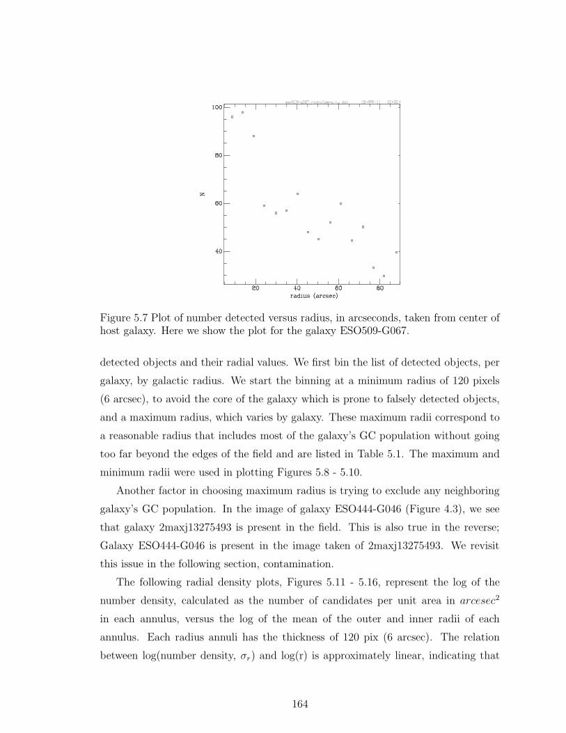
Figure 5.7 Plot of number detected versus radius, in arcseconds, taken from center ofhost galaxy. Here we show the plot for the galaxy ESO509-G067.
detected objects and their radial values. We first bin the list of detected objects, per
galaxy, by galactic radius. We start the binning at a minimum radius of 120 pixels
(6 arcsec), to avoid the core of the galaxy which is prone to falsely detected objects,
and a maximum radius, which varies by galaxy. These maximum radii correspond to
a reasonable radius that includes most of the galaxy’s GC population without going
too far beyond the edges of the field and are listed in Table 5.1. The maximum and
minimum radii were used in plotting Figures 5.8 - 5.10.
Another factor in choosing maximum radius is trying to exclude any neighboring
galaxy’s GC population. In the image of galaxy ESO444-G046 (Figure 4.3), we see
that galaxy 2maxj13275493 is present in the field. This is also true in the reverse;
Galaxy ESO444-G046 is present in the image taken of 2maxj13275493. We revisit
this issue in the following section, contamination.
The following radial density plots, Figures 5.11 - 5.16, represent the log of the
number density, calculated as the number of candidates per unit area in arcesec2
in each annulus, versus the log of the mean of the outer and inner radii of each
annulus. Each radius annuli has the thickness of 120 pix (6 arcsec). The relation
between log(number density, σr) and log(r) is approximately linear, indicating that
164
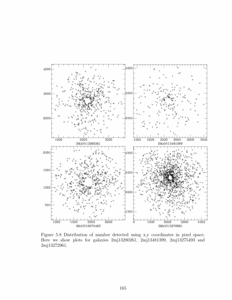
Figure 5.8 Distribution of number detected using x,y coordinates in pixel space.Here we show plots for galaxies 2mj13280261, 2mj13481399, 2mj13275493 and2mj13272961.
165

Figure 5.9 Distribution of number detected using x,y coordinates in pixel space. Herewe show plots for galaxies ESO383-G076, ESO444-G046, ESO325-G004 and ESO509-G008.
166
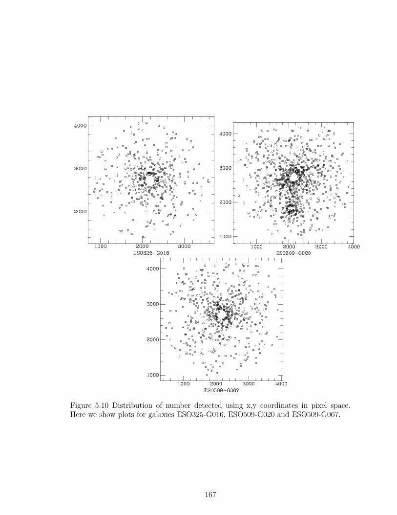
Figure 5.10 Distribution of number detected using x,y coordinates in pixel space.Here we show plots for galaxies ESO325-G016, ESO509-G020 and ESO509-G067.
167

Table 5.1. Radial Data
galaxy cluster R100(arcsec) b a rmin pix rmax pix
eso383-g076 A3571 138.3 1.229 1.151 20 2040
2mj13481399 A3571 138.3 1.030 1.949 0 1400
eso444-g046 A3558 115.3 2.041 1.653 35 1680
2mj13272961 A3558 115.3 1.234 1.480 10 2040
2mj13275493 A3558 115.3 1.147 1.460 10 1000
2mj13280261 A3558 115.3 1.327 1.771 10 1400
eso325-g004 AS0740 149.7 1.167 1.405 20 2040
eso325-g016 A3570 149.7 1.708 2.055 20 1400
eso509-g008 A1736a 149.7 1.530 1.692 20 1600
eso509-g020 A1736a 149.7 1.849 1.897 20 1800
eso509-g067 A1736a 149.7 1.165 1.612 15 1800
GCs follow a power law density distribution. The number densities are corrected for
“background”.
The best fit lines in each of the radial density plots have the form,
log(σr) = b − a(log(r)) (5.3)
The values of the minimum and maximum galactic radius used in this calculation
are listed in Table 5.1 as well as the parameters for the linear fits in the radial density
plots. The first column in the galaxy name and the second is the Abell cluster name
followed by the distance in arcseconds that equals 100 kpc. The next two columns
are the fitting parameters in equation 5.3 followed by the minimum and maximum
radii in pixels. The resolution for ACS is 20 pix/arcsec.
If you take the integral of the radial density σr with respect to radius with limits
from maximum radius to some large radius (100 kpc) to make sure we are including
168
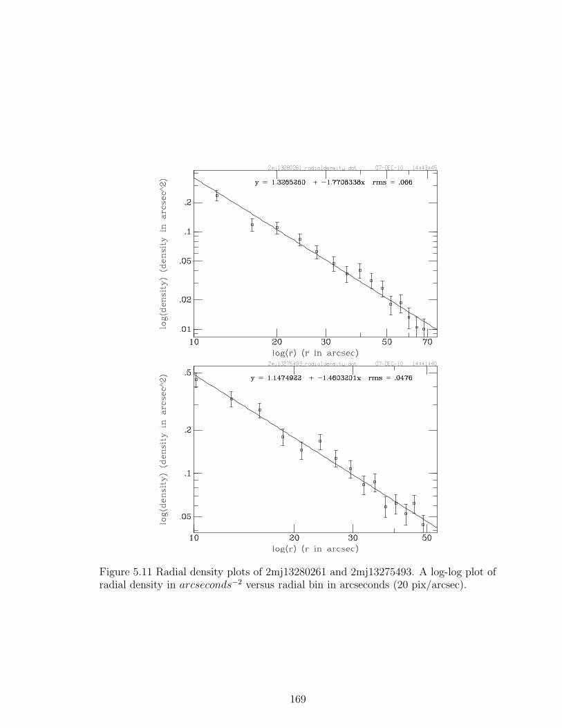
Figure 5.11 Radial density plots of 2mj13280261 and 2mj13275493. A log-log plot ofradial density in arcseconds−2 versus radial bin in arcseconds (20 pix/arcsec).
169
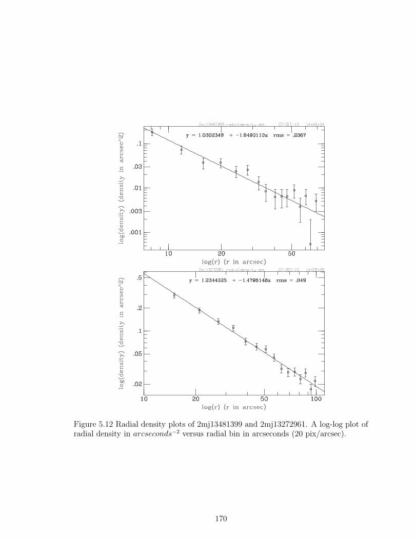
Figure 5.12 Radial density plots of 2mj13481399 and 2mj13272961. A log-log plot ofradial density in arcseconds−2 versus radial bin in arcseconds (20 pix/arcsec).
170
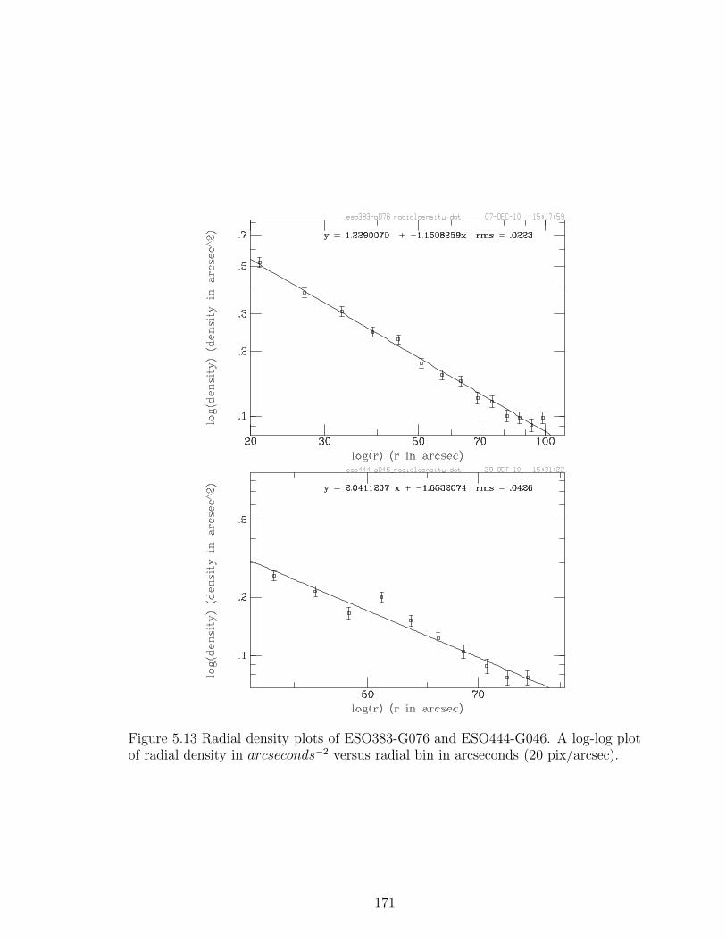
Figure 5.13 Radial density plots of ESO383-G076 and ESO444-G046. A log-log plotof radial density in arcseconds−2 versus radial bin in arcseconds (20 pix/arcsec).
171
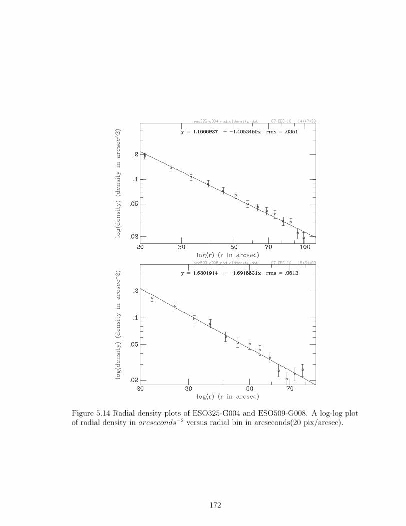
Figure 5.14 Radial density plots of ESO325-G004 and ESO509-G008. A log-log plotof radial density in arcseconds−2 versus radial bin in arcseconds(20 pix/arcsec).
172
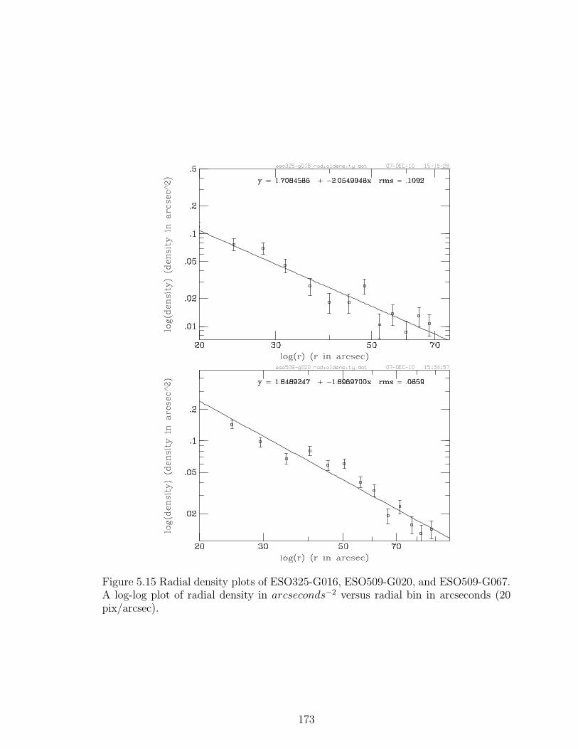
Figure 5.15 Radial density plots of ESO325-G016, ESO509-G020, and ESO509-G067.A log-log plot of radial density in arcseconds−2 versus radial bin in arcseconds (20pix/arcsec).
173
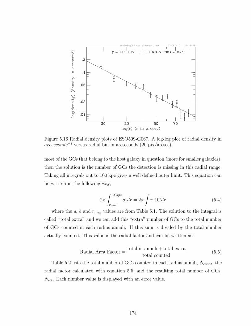
Figure 5.16 Radial density plots of ESO509-G067. A log-log plot of radial density inarcseconds−2 versus radial bin in arcseconds (20 pix/arcsec).
most of the GCs that belong to the host galaxy in question (more for smaller galaxies),
then the solution is the number of GCs the detection is missing in this radial range.
Taking all integrals out to 100 kpc gives a well defined outer limit. This equation can
be written in the following way,
2π
∫ 100kpc
rmax
σrdr = 2π
∫
ra10bdr (5.4)
where the a, b and rmax values are from Table 5.1. The solution to the integral is
called “total extra” and we can add this “extra” number of GCs to the total number
of GCs counted in each radius annuli. If this sum is divided by the total number
actually counted. This value is the radial factor and can be written as:
Radial Area Factor =total in annuli + total extra
total counted(5.5)
Table 5.2 lists the total number of GCs counted in each radius annuli, Ncount, the
radial factor calculated with equation 5.5, and the resulting total number of GCs,
Ntot. Each number value is displayed with an error value.
174
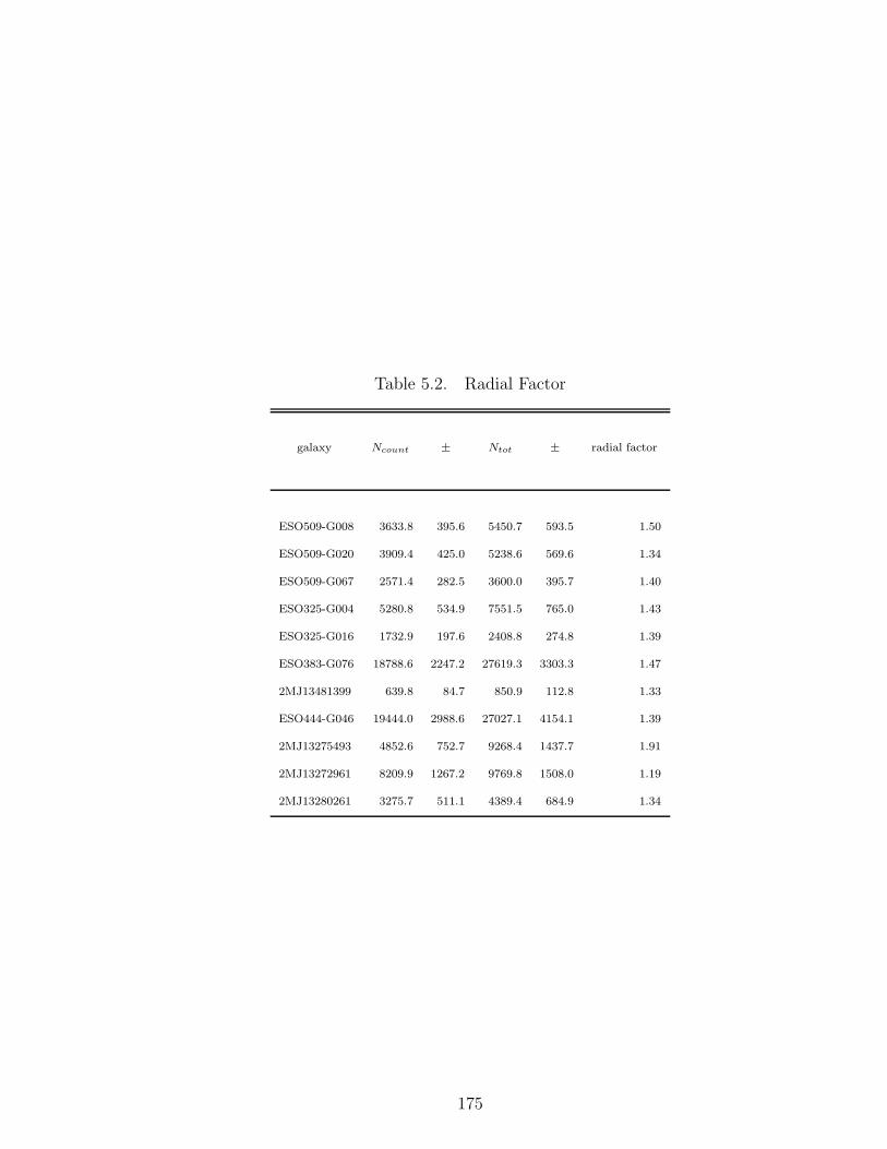
Table 5.2. Radial Factor
galaxy Ncount ± Ntot ± radial factor
ESO509-G008 3633.8 395.6 5450.7 593.5 1.50
ESO509-G020 3909.4 425.0 5238.6 569.6 1.34
ESO509-G067 2571.4 282.5 3600.0 395.7 1.40
ESO325-G004 5280.8 534.9 7551.5 765.0 1.43
ESO325-G016 1732.9 197.6 2408.8 274.8 1.39
ESO383-G076 18788.6 2247.2 27619.3 3303.3 1.47
2MJ13481399 639.8 84.7 850.9 112.8 1.33
ESO444-G046 19444.0 2988.6 27027.1 4154.1 1.39
2MJ13275493 4852.6 752.7 9268.4 1437.7 1.91
2MJ13272961 8209.9 1267.2 9769.8 1508.0 1.19
2MJ13280261 3275.7 511.1 4389.4 684.9 1.34
175
5.2.3 Contamination
In the previous sections we have shown that the proximity of 2mj13275493 to
ES0444-G046, the brightest cluster galaxy (BCG) of A3558, made it so both could be
seen in each others’ field. This made the issue of maximum radius, discussed in the
“radial factor” section, problematic. Perhaps the Ntot in 2mj13275493 is ’contami-
nated’ with GCs that belong to the BCG of A3558. We came to the conclusion that
the issue of contamination, in this study, would affect only members of Abell 3558.
Looking at Table 5.3, we can see the A3558 members are the last four galaxies. We
can also see the distance of galaxies in this study, relative to their BCGs, are less than
1 Mpc only in this cluster, with the exception of ES0509-G020. All the galaxies with
offset values of zero in Table 5.3 are the BCGs of the cluster. In A3558, the BCG,
ES0444-G046, is a giant elliptical and about twice as big as the BCG in A1736a,
ES0509-G008. ES0509-G008 is approximately the same size as the other A1736a
members (see Table 5.7 for galaxy size, RI)). This is the reason why A1736a is given
the BM type III in Table 4.2 (see Chapter 1 for BM type definition). Since we do not
survey all members in A1736a, there is a possibility there is another galaxy of compa-
rable size to ES0509-G008 even closer to ES0509-G020, therefore taking into account
the GC contamination from ES0509-G008, just because it is the BCG by being only
slighter brighter than the other members, would not be consistent. Contamination in
this study is considering contamination from a central, massive BCG.
To calculate contamination, we first look at the radial density of the BCG at
the distance of the neighbor galaxy. Looking at the radial density plots we see that
the density drops off as you get further and further from the BCG center. Since at
the distance of neighboring members of the cluster we are venturing into such low
densities, we take the radial density to be constant over the detection area of the
neighboring galaxy. We use equation 5.3 to calculate the radial density of the BCG
at this distance. We then subtract this constant density from the densities in each
radial bin already calculated during the initial radial factor process. This new binned
file has to be corrected for “contamination”, and when plotted can give us new fitting
parameters to our radial density plots (see Figures 5.17 and 5.18). The values are
176

Table 5.3. Galaxy Offsets from BCG
Galaxy Abell RA Dec geom. scale offset offset
Cluster (J2000) (J2000) (kpc/arcsec) (arcsec) (kpc)
ESO509-G008 A1736a 13:26:44.10 -27:26:21.8 0.668 0 0
ESO509-G020 A1736a 13:28:00.15 -27:21:15.5 0.668 1057.7 706.5
ESO509-G067 A1736a 13:34:47.80 -27:07:37.4 0.668 6546.8 4373.3
ESO325-G016 A3570 13:46:24.00 -37:58:15.6 0.668 0 0
ESO325-G004 AS0740 13:43:33.20 -38:10:33.7 0.668 0 0
ESO383-G076 A3571 13:47:28.40 -32:51:53.0 0.723 0 0
2MJ13481399 A3571 13:48:14.00 -33:22:54.7 0.723 1947.169 1407.8
ESO444-G046 A3558 13:27:56.86 -31:29:44.6 0.867 0 0
2MJ13275493 A3558 13:27:54.95 -31:32:18.7 0.867 156.9 136.0
2MJ13272961 A3558 13:27:29.63 -31:23:24.2 0.867 514.6 446.2
2MJ13280261 A3558 13:28:02.62 -31:45:20.8 0.867 939.9 814.9
177
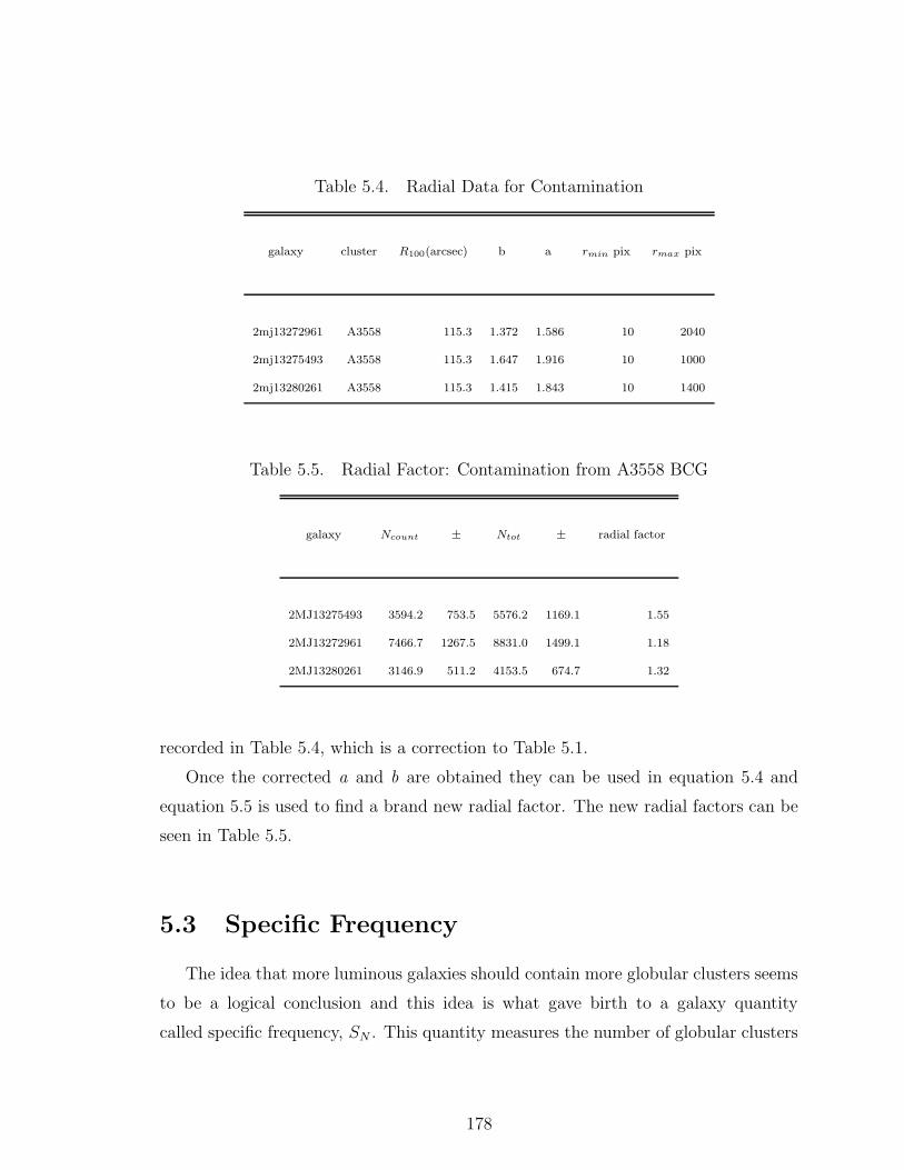
Table 5.4. Radial Data for Contamination
galaxy cluster R100(arcsec) b a rmin pix rmax pix
2mj13272961 A3558 115.3 1.372 1.586 10 2040
2mj13275493 A3558 115.3 1.647 1.916 10 1000
2mj13280261 A3558 115.3 1.415 1.843 10 1400
Table 5.5. Radial Factor: Contamination from A3558 BCG
galaxy Ncount ± Ntot ± radial factor
2MJ13275493 3594.2 753.5 5576.2 1169.1 1.55
2MJ13272961 7466.7 1267.5 8831.0 1499.1 1.18
2MJ13280261 3146.9 511.2 4153.5 674.7 1.32
recorded in Table 5.4, which is a correction to Table 5.1.
Once the corrected a and b are obtained they can be used in equation 5.4 and
equation 5.5 is used to find a brand new radial factor. The new radial factors can be
seen in Table 5.5.
5.3 Specific Frequency
The idea that more luminous galaxies should contain more globular clusters seems
to be a logical conclusion and this idea is what gave birth to a galaxy quantity
called specific frequency, SN . This quantity measures the number of globular clusters
178
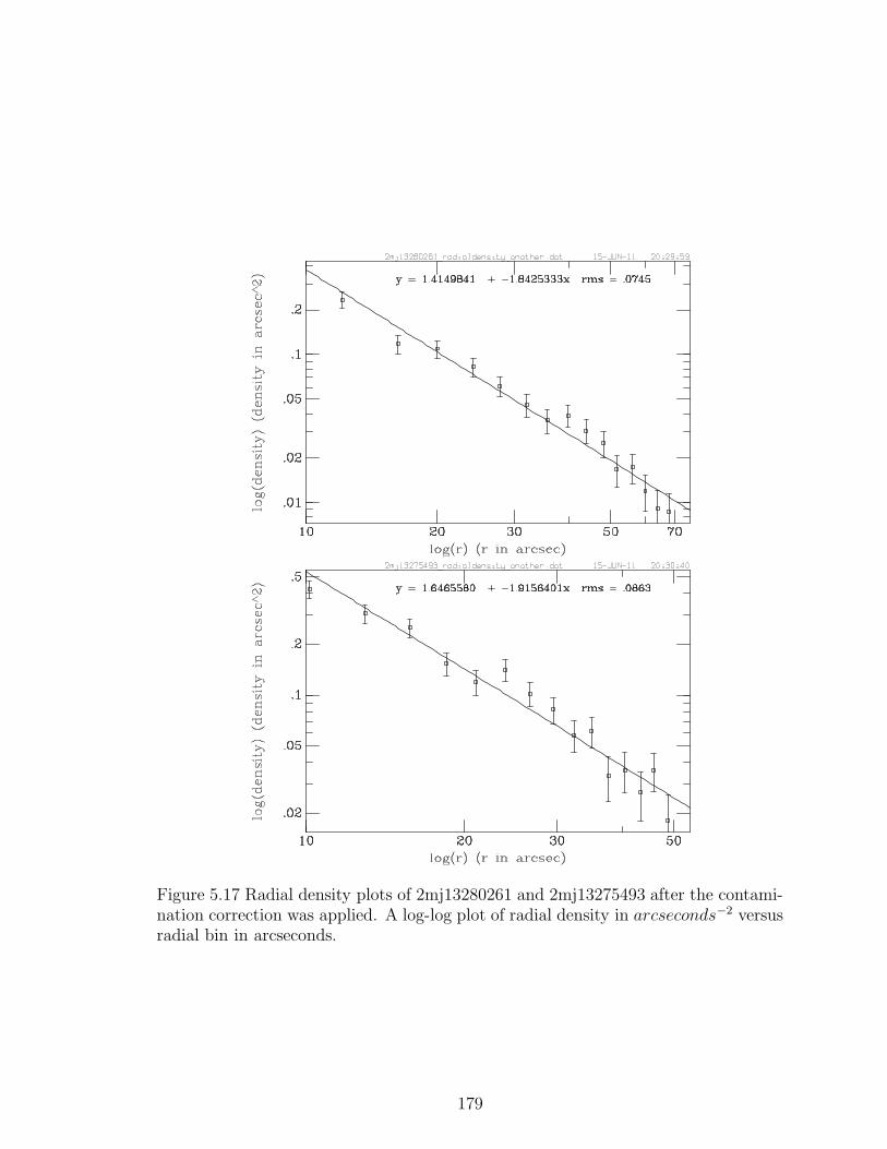
Figure 5.17 Radial density plots of 2mj13280261 and 2mj13275493 after the contami-nation correction was applied. A log-log plot of radial density in arcseconds−2 versusradial bin in arcseconds.
179
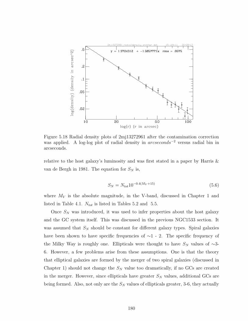
Figure 5.18 Radial density plots of 2mj13272961 after the contamination correctionwas applied. A log-log plot of radial density in arcseconds−2 versus radial bin inarcseconds.
relative to the host galaxy’s luminosity and was first stated in a paper by Harris &
van de Bergh in 1981. The equation for SN is,
SN = Ntot10−0.4(MV +15) (5.6)
where MV is the absolute magnitude, in the V-band, discussed in Chapter 1 and
listed in Table 4.1. Ntot is listed in Tables 5.2 and 5.5.
Once SN was introduced, it was used to infer properties about the host galaxy
and the GC system itself. This was discussed in the previous NGC1533 section. It
was assumed that SN should be constant for different galaxy types. Spiral galaxies
have been shown to have specific frequencies of ∼1 - 2. The specific frequency of
the Milky Way is roughly one. Ellipticals were thought to have SN values of ∼3-
6. However, a few problems arise from these assumptions. One is that the theory
that elliptical galaxies are formed by the merger of two spiral galaxies (discussed in
Chapter 1) should not change the SN value too dramatically, if no GCs are created
in the merger. However, since ellipticals have greater SN values, additional GCs are
being formed. Also, not only are the SN values of ellipticals greater, 3-6, they actually
180
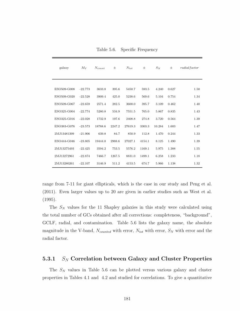
Table 5.6. Specific Frequency
galaxy MV Ncount ± Ntot ± SN ± radialfactor
ESO509-G008 -22.773 3633.8 395.6 5450.7 593.5 4.240 0.627 1.50
ESO509-G020 -22.528 3909.4 425.0 5238.6 569.6 5.104 0.754 1.34
ESO509-G067 -22.659 2571.4 282.5 3600.0 395.7 3.109 0.462 1.40
ESO325-G004 -22.774 5280.8 534.9 7551.5 765.0 5.867 0.835 1.43
ESO325-G016 -22.028 1732.9 197.6 2408.8 274.8 3.720 0.564 1.39
ESO383-G076 -23.573 18788.6 2247.2 27619.3 3303.3 10.284 1.603 1.47
2MJ13481399 -21.906 639.8 84.7 850.9 112.8 1.470 0.244 1.33
ESO444-G046 -23.805 19444.0 2988.6 27027.1 4154.1 8.125 1.490 1.39
2MJ13275493 -22.425 3594.2 753.5 5576.2 1169.1 5.975 1.388 1.55
2MJ13272961 -22.874 7466.7 1267.5 8831.0 1499.1 6.258 1.233 1.18
2MJ13280261 -22.107 3146.9 511.2 4153.5 674.7 5.966 1.138 1.32
range from 7-11 for giant ellipticals, which is the case in our study and Peng et al.
(2011). Even larger values up to 20 are given in earlier studies such as West et al.
(1995).
The SN values for the 11 Shapley galaxies in this study were calculated using
the total number of GCs obtained after all corrections: completeness, “background”,
GCLF, radial, and contamination. Table 5.6 lists the galaxy name, the absolute
magnitude in the V-band, Ncounted with error, Ntot with error, SN with error and the
radial factor.
5.3.1 SN Correlation between Galaxy and Cluster Properties
The SN values in Table 5.6 can be plotted versus various galaxy and cluster
properties in Tables 4.1 and 4.2 and studied for correlations. To give a quantitative
181

value for visual trends, we use the Spearman and Pearson estimates for the significance
of the correlation. These estimates are described in Numerical Recipes (Press et al.
1992). When Pearson’s r (also called the linear correlation coefficient) equals 1, it
is said to be in “complete positive correlation” where the data points form a linear
relation with a positive slope. The Pearson’s r ranges from -1 to 1, with negative
values relating to negative slopes for the trend line. The Spearman rank correlation
coefficient also ranges from -1 or 1 and like Pearson’s value represents correlation
when the value is very near 1. For the rest of the thesis, we will call the Spearman
rank correlation coefficient, s correlation, and Pearson’s r, p correlation.
Galaxy Properties
In this section we investigate how SN scales with MV , radial velocity, cz and
velocity dispersion of the host galaxy (see Table 4.1). As discussed in the magnitude
section of Chapter 1, MV is the absolute V-band magnitude of the host galaxy. It can
be calculated from the distance modulus, DM, and the apparent magnitude, mV , of
the galaxy. The distance modulus, DM = mV - MV , used for each galaxy is that of
the associated cluster to avoid any effect from the internal velocities of the member
galaxies. The distance modulus can be calculated by assuming standard cosmological
parameters, H0 = 73 km/s Mpc−1. Peng et al. (2008) mentioned a relation between
MV and Specific frequency with low and high magnitudes increasing in SN with
intermediate magnitudes having lower SN , forming a kind of U shape. Looking at
Figure 5.19, which only contains 11 galaxies, we do not see a slight U shape. However,
we do see a trend of increasing SN with increasing magnitude. The s correlation is
0.98 and the p correlation is > 0.99. The trend is less apparent when looking at the
BCGs, the circles in the plot; however, it does reduce the sample points. When one
considers that the outliers are galaxy members farther away from the cluster center,
the idea of GCs being associated with the galaxy and/or the cluster can materialize.
There should be no correlation between radial velocity and SN . A possible cor-
relation in a SN versus cz plot would be from some systematic error. When SN is
compared to radial velocity, cz, of each galaxy in Figure 5.20, no trend can be seen.
182
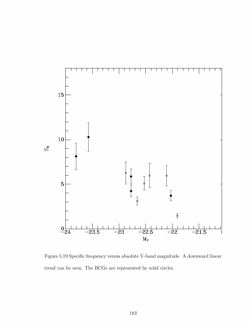
Figure 5.19 Specific frequency versus absolute V-band magnitude. A downward linear
trend can be seen. The BCGs are represented by solid circles.
183

The BCGs were plotted as circles in the plot but there is also no correlation between
SN of the BCGs.
Velocity dispersions for 10 out of 11 galaxies were found in the literature and
recorded in Table 4.1. The velocity dispersion of galaxies is usually derived from ana-
lyzing shifts and broadening of the absorption lines in galaxy spectra. The variations
in the absorption lines are due to the orbital motions of the stars that reside in the
galaxy and therefore contribute to the galaxy spectrum (Binney 1998). Figure 5.21
shows an approximately linear trend with greater values of galaxy velocity disper-
sion, σgal, corresponding to greater SN values. The s correlation is 0.97 and the p
correlation is 0.94.
Using the virial theorem, in 3D space, the velocity dispersion can be related to
the galaxy mass the following way,
1
2m(3σ)2 =
GmM(R)
R(5.7)
where the m is mass of a single star (negligible compared to the mass of the galaxy),
M is the mass of the galaxy (or star cluster in question), and G is the gravitational
constant. Since a correlation between specific frequency and the mass of galaxy
is reasonable (bigger galaxy, more GCs), and σ depends on the mass, the trend in
Figure 5.21 is not surprising. Equation 5.7 claims that σ2gal is proportional to M(R)
R, but
the functional form of M(R) is uncertain. However, virial analyses (e.g., Cappellari
et al. 2006; Mo, van den Bosch & White 2010) indicate that a galaxy’s gravitating
mass is proportional to σ2Re, where σ is the central stellar velocity dispersion, and Re
is the effective radius. For similar types of galaxies, effective radii are closely related
to the isophotal radii, which are much easier to measure observationally. Table 5.7
presents values of the isophotal radius RI , which is the linear size in arcsec out to an
I-band isophote of 22.5 mag/arcsec2. These values were retrieved from the Hyperleda
website, a database for physics of galaxies (http://leda.univ-lyon1.fr/). The RI values
in arcsec are then converted to a physical size in kpc, taking into account the cluster
distances. The conversion factors for the clusters are included in Table 5.7. The Table
also repeats the SN values for each galaxy.
184
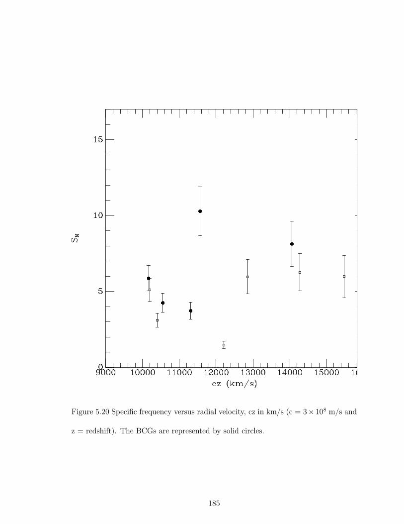
Figure 5.20 Specific frequency versus radial velocity, cz in km/s (c = 3× 10⁸ m/s and
z = redshift). The BCGs are represented by solid circles.
185
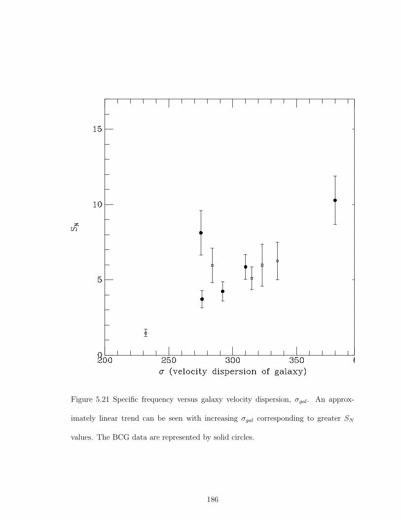
Figure 5.21 Specific frequency versus galaxy velocity dispersion, σgal. An approx-
imately linear trend can be seen with increasing σgal corresponding to greater SN
values. The BCG data are represented by solid circles.
186
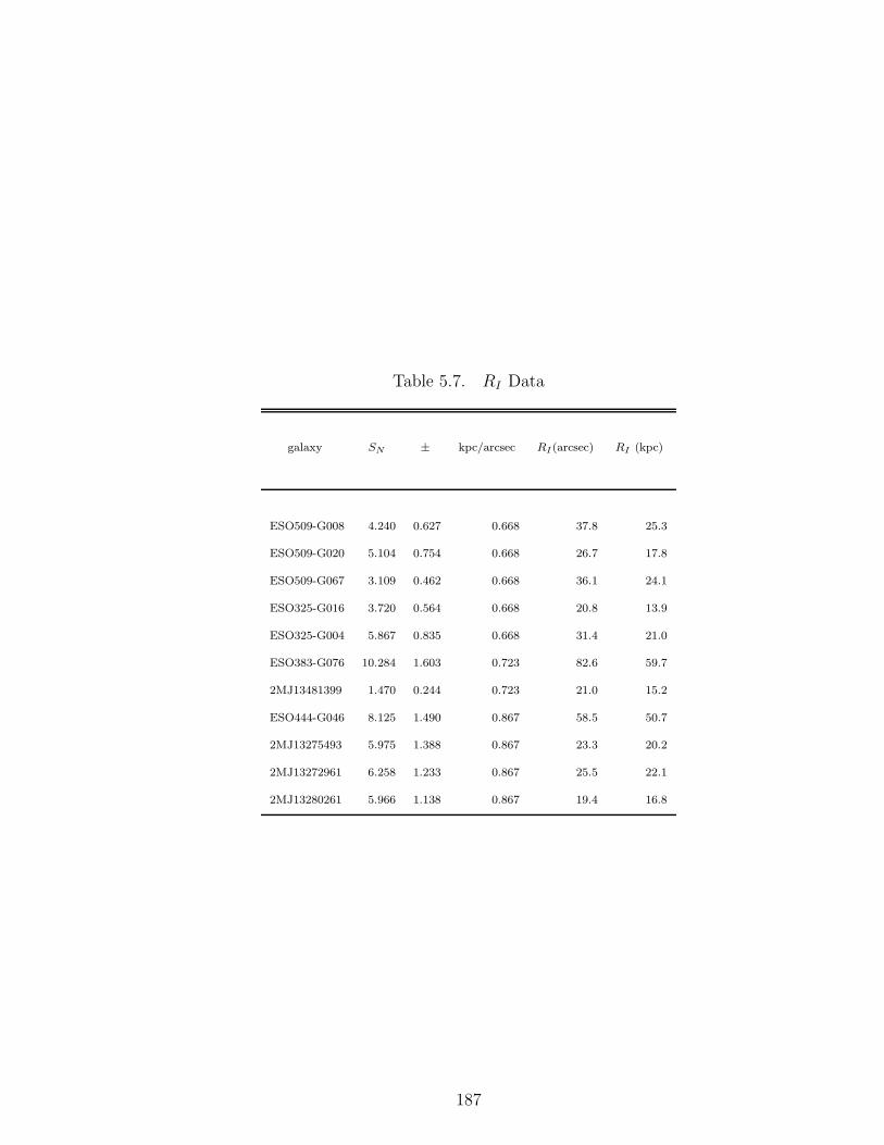
Table 5.7. RI Data
galaxy SN ± kpc/arcsec RI(arcsec) RI (kpc)
ESO509-G008 4.240 0.627 0.668 37.8 25.3
ESO509-G020 5.104 0.754 0.668 26.7 17.8
ESO509-G067 3.109 0.462 0.668 36.1 24.1
ESO325-G016 3.720 0.564 0.668 20.8 13.9
ESO325-G004 5.867 0.835 0.668 31.4 21.0
ESO383-G076 10.284 1.603 0.723 82.6 59.7
2MJ13481399 1.470 0.244 0.723 21.0 15.2
ESO444-G046 8.125 1.490 0.867 58.5 50.7
2MJ13275493 5.975 1.388 0.867 23.3 20.2
2MJ13272961 6.258 1.233 0.867 25.5 22.1
2MJ13280261 5.966 1.138 0.867 19.4 16.8
187
Figure 5.22 shows that both SN and the total number of GCs depend on the
galaxy mass. The top panel of Figure 5.22 plots specific frequency versus the log
of the product of galaxy velocity dispersion squared σ2gal and RI , which should be
proportional to the galaxy mass. The bottom panel shows a log-log plot of Ntot
versus the same quantity along the x-axis as in the top panel.
Cluster Properties
Now we will look at the correlation between SN and the properties of the cluster
in which the host galaxy resides. The cluster properties recorded in Table 4.2 are,
the cluster velocity dispersions, the type of cluster, and the Abell count, or richness,
of the cluster. The velocity dispersion of a cluster, σ, is the standard deviation of the
radial velocities, cz, of all the cluster members. As Chap 4 states, these σ values are
obtained from various sources of literature except for AS0740 which was calculated
by collecting the radial velocities of all members. The cluster velocity dispersion for
ESO509-G067 could not be found. We see a slight trend upward in the SN versus
velocity dispersion plot, Figure 5.23. The s correlation is 0.92 and the p correlation is
0.78. These values can not confirm strong correlation. However, this trend would be
even more prominent if 2MJ13481399 point was excluded. 2MJ13481399 is interesting
in the sense that its low GC population, which is the main factor for a small SN of
1.47, may be due to its distant location to the cluster center. This issue will be
revisited in section 5.5. If the galaxy had a bigger GC population then it would fall
in the upward trend. The other galaxy in this study that occupies the same cluster
as 2MJ13481399 is ESO383-G076 and it has a much more abundant GC population.
This upward trend is discussed in Blakeslee et al. (1999), Elmgreen (1999), Harris et
al. (1998) and is even more present in the BCGs. When considering only the BCGs
in Figure 5.23, the p correlation rises significantly to 0.92, which makes sense since
most of the BCGs are located at the cluster center (see section 5.5).
As stated in Chapter 1, the Bautz-Morgan Type, BM type, is related to the
morphology of the cluster. A cluster with a BM type of I has a single supergiant cD
galaxy and a BM type of III indicates a cluster where the one member is no bigger
188
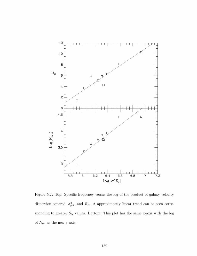
Figure 5.22 Top: Specific frequency versus the log of the product of galaxy velocity
dispersion squared, σ2gal, and RI . A approximately linear trend can be seen corre-
sponding to greater SN values. Bottom: This plot has the same x-axis with the log
of Ntot as the new y-axis.
189

Figure 5.23 Specific frequency versus cluster velocity dispersion. The BCGs are plot-
ted as solid circles. Value could not be found for ESO509-G067.
190
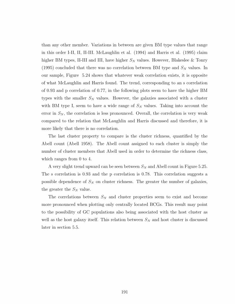
than any other member. Variations in between are given BM type values that range
in this order I-II, II, II-III. McLaughlin et al. (1994) and Harris et al. (1995) claim
higher BM types, II-III and III, have higher SN values. However, Blakeslee & Tonry
(1995) concluded that there was no correlation between BM type and SN values. In
our sample, Figure 5.24 shows that whatever weak correlation exists, it is opposite
of what McLaughlin and Harris found. The trend, corresponding to an s correlation
of 0.93 and p correlation of 0.77, in the following plots seem to have the higher BM
types with the smaller SN values. However, the galaxies associated with a cluster
with BM type I, seem to have a wide range of SN values. Taking into account the
error in SN , the correlation is less pronounced. Overall, the correlation is very weak
compared to the relation that McLaughlin and Harris discussed and therefore, it is
more likely that there is no correlation.
The last cluster property to compare is the cluster richness, quantified by the
Abell count (Abell 1958). The Abell count assigned to each cluster is simply the
number of cluster members that Abell used in order to determine the richness class,
which ranges from 0 to 4.
A very slight trend upward can be seen between SN and Abell count in Figure 5.25.
The s correlation is 0.93 and the p correlation is 0.78. This correlation suggests a
possible dependence of SN on cluster richness. The greater the number of galaxies,
the greater the SN value.
The correlations between SN and cluster properties seem to exist and become
more pronounced when plotting only centrally located BCGs. This result may point
to the possibility of GC populations also being associated with the host cluster as
well as the host galaxy itself. This relation between SN and host cluster is discussed
later in section 5.5.
191

Figure 5.24 Specific frequency versus BM type. We conclude there is no trend con-
sidering error in SN . The BCGs are plotted as solid circles.
192
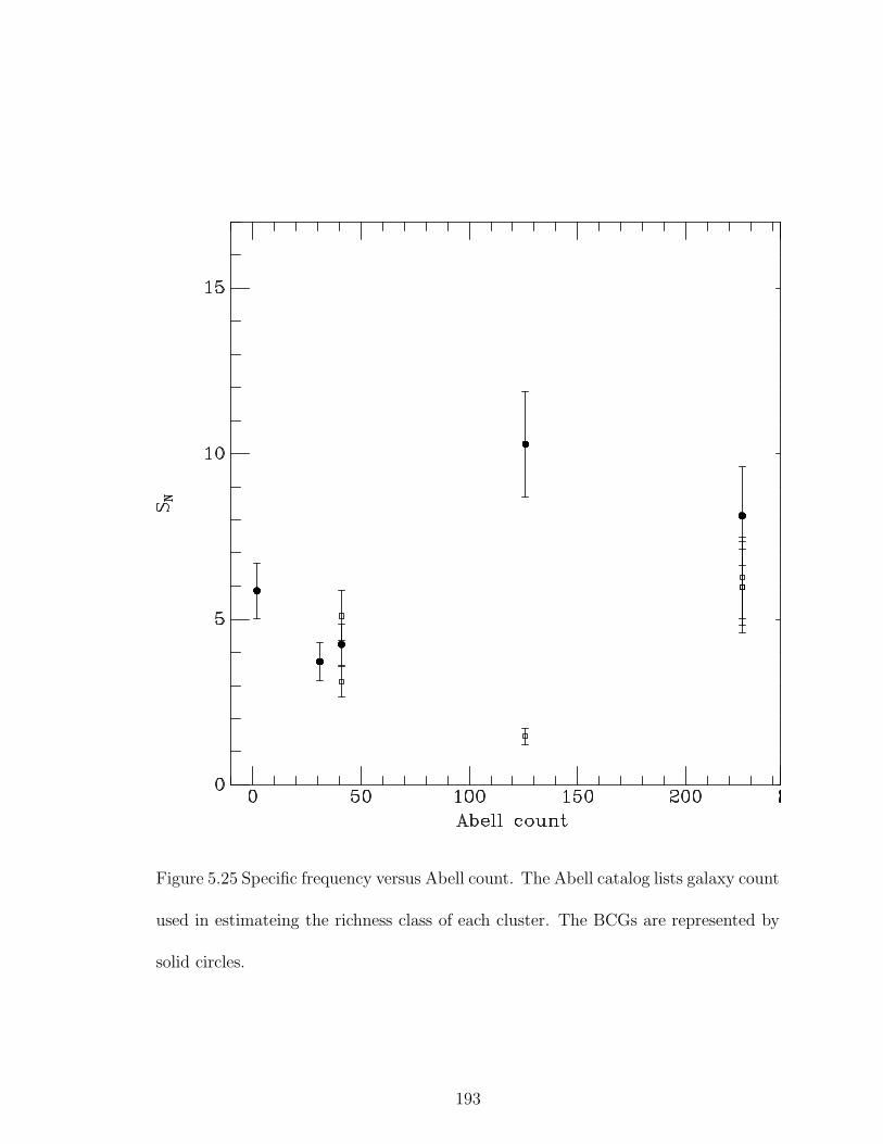
Figure 5.25 Specific frequency versus Abell count. The Abell catalog lists galaxy count
used in estimateing the richness class of each cluster. The BCGs are represented by
solid circles.
193
5.4 Total Number of GCs and Host Galaxy Lumi-
nosity Relation
Early on in galactic astronomy, it was thought that the number of GCs should
roughly scale with the host galaxy’s stellar luminosity, which was discussed earlier as
one of the notions that helped develop the equation for specific frequency. However,
the SN versus MV plot (Figure 5.19) showed a slight downward trend that led us to
investigate a more fundamental idea of just total number of GCs, N, versus optical
luminosity of the galaxy, L. We can obtain absolute luminosity, LV , using our MV
values (listed in Table 5.6)and the following equation,
MV = −2.5logLV + C (5.8)
where C is the MV value of the sun, 4.83. When equation 5.8 is solved for log(LV ),
one finds it is proportional to -0.4*MV . To look for a correlation, we plot log(N)
versus log(LV ) in Figure 5.26.
We see a good relation between log(N) and log(LV ) described by the following
equation:
logN = −10.7 + 1.59logLV (5.9)
which scales with luminosity to the power of 1.6.
5.5 Intracluster Globular Clusters
The formation scenario described in Chapter 1 discussed the problem with the
simple notion that if ellipticals are merged spirals then they should have SN values
the same as spiral galaxies, SN ∼2. Peng et al. (2008) shows that there are indeed
ellipticals with this value but there also exist a wide range of SN values that get
into the teens. This issue of high SN values was studied in West et al, (1995), where
they believed the issue had to do with “Intracluster Globular Clusters” (IGCs). They
194
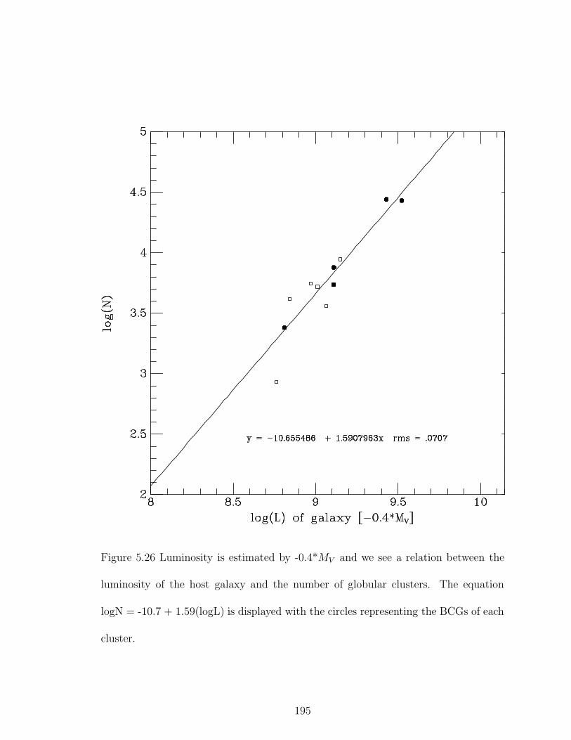
Figure 5.26 Luminosity is estimated by -0.4*MV and we see a relation between the
luminosity of the host galaxy and the number of globular clusters. The equation
logN = -10.7 + 1.59(logL) is displayed with the circles representing the BCGs of each
cluster.
195
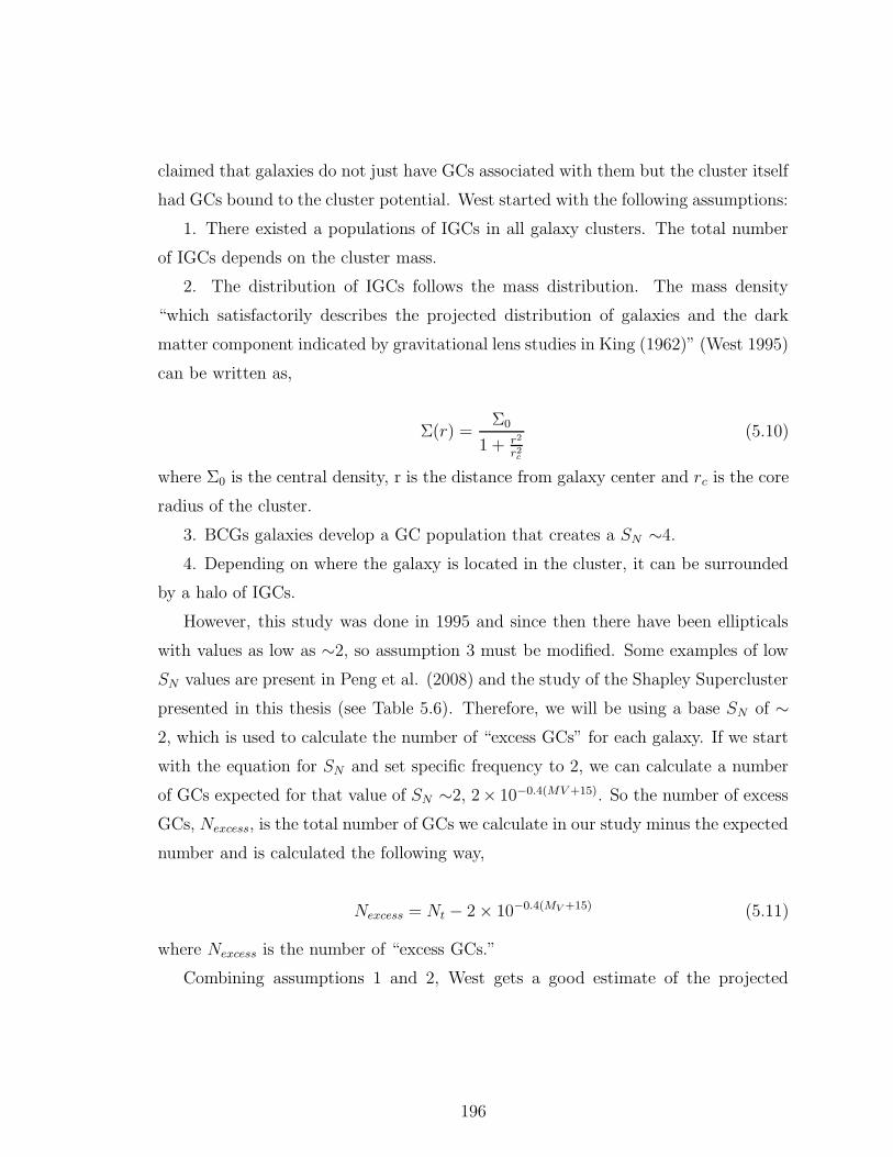
claimed that galaxies do not just have GCs associated with them but the cluster itself
had GCs bound to the cluster potential. West started with the following assumptions:
1. There existed a populations of IGCs in all galaxy clusters. The total number
of IGCs depends on the cluster mass.
2. The distribution of IGCs follows the mass distribution. The mass density
“which satisfactorily describes the projected distribution of galaxies and the dark
matter component indicated by gravitational lens studies in King (1962)” (West 1995)
can be written as,
Σ(r) =Σ0
1 + r2
r2c
(5.10)
where Σ0 is the central density, r is the distance from galaxy center and rc is the core
radius of the cluster.
3. BCGs galaxies develop a GC population that creates a SN ∼4.
4. Depending on where the galaxy is located in the cluster, it can be surrounded
by a halo of IGCs.
However, this study was done in 1995 and since then there have been ellipticals
with values as low as ∼2, so assumption 3 must be modified. Some examples of low
SN values are present in Peng et al. (2008) and the study of the Shapley Supercluster
presented in this thesis (see Table 5.6). Therefore, we will be using a base SN of ∼2, which is used to calculate the number of “excess GCs” for each galaxy. If we start
with the equation for SN and set specific frequency to 2, we can calculate a number
of GCs expected for that value of SN ∼2, 2× 10−0.4(MV +15). So the number of excess
GCs, Nexcess, is the total number of GCs we calculate in our study minus the expected
number and is calculated the following way,
Nexcess = Nt − 2 × 10−0.4(MV +15) (5.11)
where Nexcess is the number of “excess GCs.”
Combining assumptions 1 and 2, West gets a good estimate of the projected
196
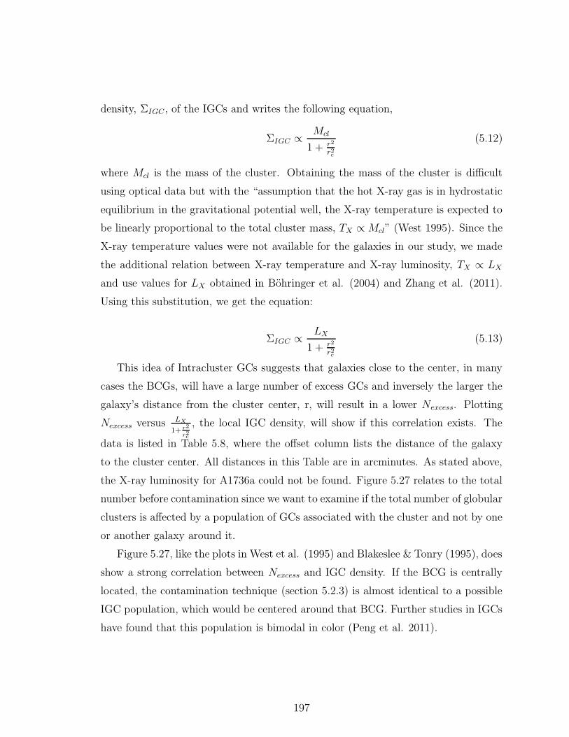
density, ΣIGC , of the IGCs and writes the following equation,
ΣIGC ∝ Mcl
1 + r2
r2c
(5.12)
where Mcl is the mass of the cluster. Obtaining the mass of the cluster is difficult
using optical data but with the “assumption that the hot X-ray gas is in hydrostatic
equilibrium in the gravitational potential well, the X-ray temperature is expected to
be linearly proportional to the total cluster mass, TX ∝ Mcl” (West 1995). Since the
X-ray temperature values were not available for the galaxies in our study, we made
the additional relation between X-ray temperature and X-ray luminosity, TX ∝ LX
and use values for LX obtained in Bohringer et al. (2004) and Zhang et al. (2011).
Using this substitution, we get the equation:
ΣIGC ∝ LX
1 + r2
r2c
(5.13)
This idea of Intracluster GCs suggests that galaxies close to the center, in many
cases the BCGs, will have a large number of excess GCs and inversely the larger the
galaxy’s distance from the cluster center, r, will result in a lower Nexcess. Plotting
Nexcess versus LX
1+ r2
r2c
, the local IGC density, will show if this correlation exists. The
data is listed in Table 5.8, where the offset column lists the distance of the galaxy
to the cluster center. All distances in this Table are in arcminutes. As stated above,
the X-ray luminosity for A1736a could not be found. Figure 5.27 relates to the total
number before contamination since we want to examine if the total number of globular
clusters is affected by a population of GCs associated with the cluster and not by one
or another galaxy around it.
Figure 5.27, like the plots in West et al. (1995) and Blakeslee & Tonry (1995), does
show a strong correlation between Nexcess and IGC density. If the BCG is centrally
located, the contamination technique (section 5.2.3) is almost identical to a possible
IGC population, which would be centered around that BCG. Further studies in IGCs
have found that this population is bimodal in color (Peng et al. 2011).
197

Figure 5.27 GC excess versus a ratio involving X-ray luminosity and core radius of
the galaxy cluster.
198

Table 5.8. Intracluster Data
galaxy cluster rc (arcmin) LX E44 erg/s offset (arcmin) Ntot ± excess LX
1+ r2
r2c
ESO325-G016 A3570 6.0 0.191 8.077 2408.8 274.8 1113.9 0.0679
ESO444-G046 A3558 6.0 5.56 0.443 27027.1 4154.1 20373.9 3.4990
2MJ13275493 A3558 6.0 5.56 2.236 9268.4 1437.7 7401.9 3.0889
2MJ13272961 A3558 6.0 5.56 8.986 9769.8 1508.0 6947.3 1.0849
2MJ13280261 A3558 6.0 5.56 15.239 4389.4 684.9 2996.8 0.4722
ESO383-G076 A3571 3.5 4.91 0.917 27619.3 3303.3 22246.1 3.9360
2MJ13481399 A3571 3.5 4.91 33.330 850.9 112.8 -306.4 0.0459
5.6 Conclusion
We present a brief introduction of the Shapley Supercluster and its connection
to the Great Attractor. The motivation for the imaging of the 11 galaxies in this
survey was to obtain velocities of each of these galaxies to further investigate the
motion toward the Great Attractor. We then list properties, from the literature, of
each galaxy imaged and the cluster in which they reside.
The data analysis using DAOphot was described in detail, from source detection
to the final corrections that needed to be applied to get a total number of globular
clusters. The total number of GCs associated with each galaxy, in Table 5.6, has
been corrected for completeness, background, luminosity function, radial distribution
and contamination from the central BCG in A3558. Table 5.6 also shows the largest
specific frequency, 10.3, to belong to ESO383-G076. This is most massive galaxy
in our survey (see Table 5.7) and along with the next largest galaxy ESO444-G046,
may be the largest GC populations studied at ∼23,000 - 30,000 (taking into account
error). However, their largest SN values may have something to do with distance
from cluster center. In Table 5.8, the total numbers are corrected for completeness,
199

background, radial affects but not contamination. We can see that the numbers all
scale with the distance from the cluster center.
We find that both galaxy and cluster properties correlate with SN . Our SN values
strongly correlate with velocity dispersion of the host galaxy, which is predicted using
the virial theorem. Since mass is proportional to σ2Re, we find a strong correlation
of SN with the dynamical mass of the galaxy in Figure 5.22. This finding agrees with
the correlation between SN and mass of the central black hole in Harris & Harris
(2011) because the central black hole mass has been found to correlate with galaxy
mass in Ferrarese (2002) and Ferrarese et al.(2006).
We find, in our 11 galaxy sample, the relation between total number of GCs and
optical galaxy luminosity varies as,
Ntot ∝ L1.6V (5.14)
where the power 1.6 suggests that the number of GCs can not be scaled with the host
galaxy luminosity. This result may suggest that GCs are not entirely associated with
the host galaxy.
The range of specific frequency values may point to GC association to host cluster
as well the host galaxy. Cross referencing Table 5.8 and Table 5.7, we see that the
galaxies with the highest SN values were not only the biggest galaxies, ESO383-G076
and ESO444-G046, but the most centrally located. There are two factors here so the
association with the cluster is not conclusive. However, the galaxy with the lowest
specific frequency of 1.47 ± 0.24 is 2MJ13481399, which is the galaxy that is the
furthest away from its host cluster center. The notion that number of GCs scales with
size of galaxy may not be totally accurate because 2MJ13481399 is not the smallest
galaxy in the survey. The smallest galaxy is ESO325-G016 and its SN value is 3.72 ±0.56. This is the third smallest specific frequency. The galaxy ESO509-G067, almost
twice as big as ESO325-G016, has a lower SN of 3.11 ± 0.46. Taking into account
error, the SN values of ESO325-G016 and ESO509-G067 may be equivalent, but the
great difference in size suggests that environment as well as size plays a role in GC
population and consequently formation.
200
Another interesting finding is the evidence, seen in Figure 5.27, for Intracluster
GCs in four of our five Abell clusters. Abell 1736a lacked LX data. Interacluster GCs
(IGCs) may be the solution to phenomenon in the previous paragraph. The large
numbers of GCs for ESO383-G076 and ESO444-G046 may be due to the addition of
IGCs, since both are within 1 arcmin of their cluster centers. The idea that clusters
have GC populations associated with them, gives clues into formation scenarios. IGCs
might be produced during mergers. They may be a result of tidally stripped GCs
that become attracted to the cluster potential or newly formed during the merger.
More studies need to be done on GC systems in clusters of varying richness.
201

Bibliography
[1] Abell, G. O. 1958, ApJS, 3, 211
[2] Blakeslee, J. P., & Tonry, J. L. 1995, ApJ, 442, 579
[7] Binney, J., & Merrifield, M. 1998, Galactic astronomy / James Binney and Michael
Merrifield. Princeton, NJ : Princeton University Press, 1998. (Princeton series in
astrophysics) QB857 .B522 1998
[4] Bohringer, H., et al. 2004, A&A, 425, 367
[6] Brodie, J. P., & Strader, J. 2006, ARA&A, 44, 193
[6] Cappellari, M., et al. 2006, MNRAS, 366, 1126
[7] Elmegreen, B. G. 1999, Ap&SS, 269, 469
[8] Ferrarese, L. 2002, ApJ, 578, 90
[9] Ferrarese, L., et al. 2006, ApJ, 644, L21
[10] Harris, W. E., & van den Bergh, S. 1981, AJ, 86, 1627
[11] Harris, W. E., Pritchet, C. J., & McClure, R. D. 1995, ApJ, 441, 120
[12] Harris, W. E., Harris, G. L. H., & McLaughlin, D. E. 1998, AJ, 115, 1801
[13] Harris, G. L. H., & Harris, W. E. 2011, MNRAS, 410, 2347
[14] King, I. 1962, AJ, 67, 471
202

[15] Peng, E. W., et al. 2008, ApJ, 681, 197
[16] Peng, E. W., et al. 2011, ApJ, 730, 23
[17] Press, W. H., Teukolsky, S. A., Vetterling, W. T., & Flannery, B. P. 1992,
Cambridge: University Press, —c1992, 2nd ed.,
[18] McLaughlin, D. E., Harris, W. E., & Hanes, D. A. 1994, ApJ, 422, 486
[19] Mo, H., van den Bosch, F. C., & White, S. 2010, Galaxy Formation and Evolu-
tion, Cambridge University Press, 2010. ISBN: 9780521857932,
[20] van den Bergh, S., & Harris, W. E. 1982, AJ, 87, 494
[21] West, M. J., Cote, P., Jones, C., Forman, W., & Marzke, R. O. 1995, ApJ, 453,
L77
[22] West, M. J., Jordan, A., Blakeslee, J. P., Cote, P., Gregg, M. D., Takamiya, M.,
& Marzke, R. O. 2011, A&A, 528, A115
[23] Zhang, Y.-Y., Andernach, H., Caretta, C. A., Reiprich, T. H., Bohringer, H.,
Puchwein, E., Sijacki, D., & Girardi, M. 2011, A&A, 526, A105
203
Chapter 6
Three Band Imaging of the
Globular Cluster Subpopulations
of ESO325-G004
6.1 Data and Selection
ESO325-G004’s UCD population was the subject of Chapter 3. As discussed in
that chapter, out of the 11 galaxies in the survey, ESO325-G004 was imaged with the
ACS/WFC in the F475W, F625W and F814W filters due to interest for a Hubble
Heritage public release image. Object detection and subsequent data reduction by
DAOphot in Chapter 4 was combined with object detection by SExtractor to ob-
tain the best GC candidates for this host galaxy. The SExtrator data was processed
previously for a study of Ultra Compact Dwarf objects discussed in Chapter 3. SEx-
tractor detects objects by finding peaks in the image and neighboring pixels that are
significantly above the local background. This detection software has a variation of
204
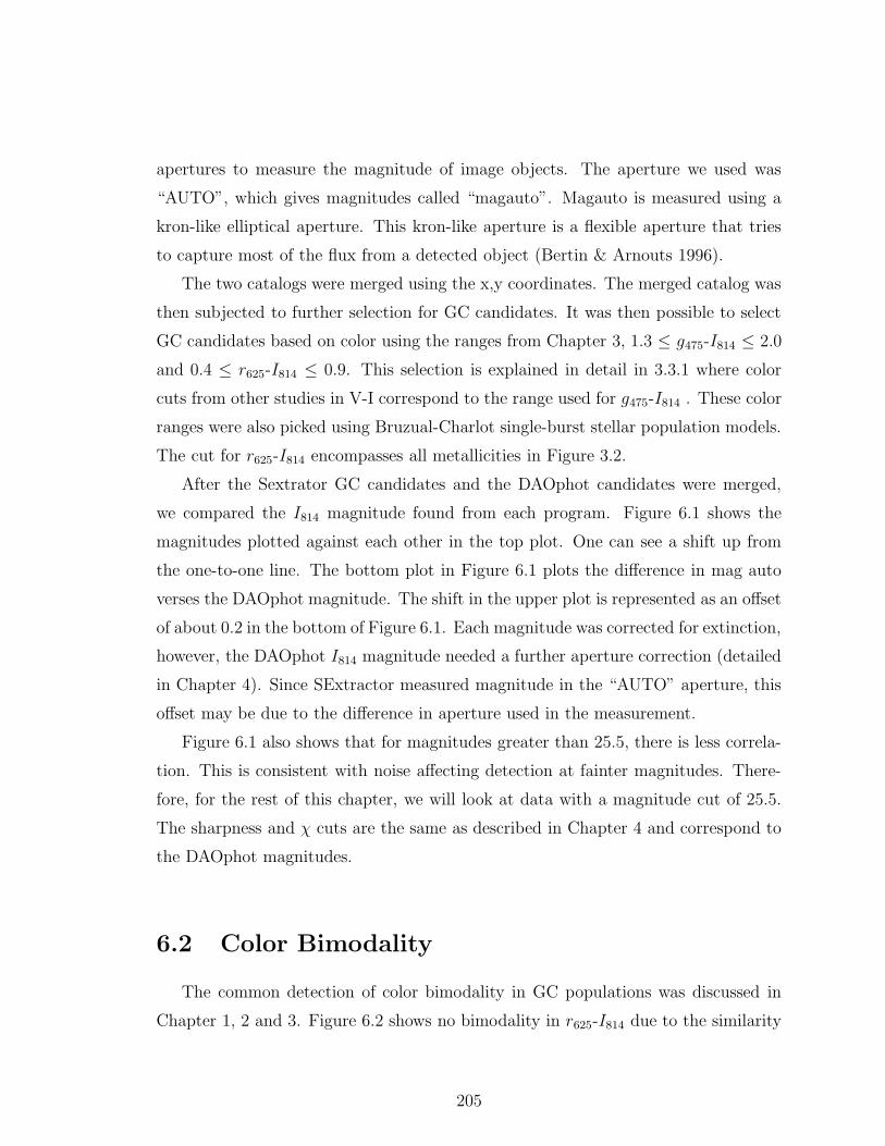
apertures to measure the magnitude of image objects. The aperture we used was
“AUTO”, which gives magnitudes called “magauto”. Magauto is measured using a
kron-like elliptical aperture. This kron-like aperture is a flexible aperture that tries
to capture most of the flux from a detected object (Bertin & Arnouts 1996).
The two catalogs were merged using the x,y coordinates. The merged catalog was
then subjected to further selection for GC candidates. It was then possible to select
GC candidates based on color using the ranges from Chapter 3, 1.3 ≤ g475-I814 ≤ 2.0
and 0.4 ≤ r625-I814 ≤ 0.9. This selection is explained in detail in 3.3.1 where color
cuts from other studies in V-I correspond to the range used for g475-I814 . These color
ranges were also picked using Bruzual-Charlot single-burst stellar population models.
The cut for r625-I814 encompasses all metallicities in Figure 3.2.
After the Sextrator GC candidates and the DAOphot candidates were merged,
we compared the I814 magnitude found from each program. Figure 6.1 shows the
magnitudes plotted against each other in the top plot. One can see a shift up from
the one-to-one line. The bottom plot in Figure 6.1 plots the difference in mag auto
verses the DAOphot magnitude. The shift in the upper plot is represented as an offset
of about 0.2 in the bottom of Figure 6.1. Each magnitude was corrected for extinction,
however, the DAOphot I814 magnitude needed a further aperture correction (detailed
in Chapter 4). Since SExtractor measured magnitude in the “AUTO” aperture, this
offset may be due to the difference in aperture used in the measurement.
Figure 6.1 also shows that for magnitudes greater than 25.5, there is less correla-
tion. This is consistent with noise affecting detection at fainter magnitudes. There-
fore, for the rest of this chapter, we will look at data with a magnitude cut of 25.5.
The sharpness and χ cuts are the same as described in Chapter 4 and correspond to
the DAOphot magnitudes.
6.2 Color Bimodality
The common detection of color bimodality in GC populations was discussed in
Chapter 1, 2 and 3. Figure 6.2 shows no bimodality in r625-I814 due to the similarity
205
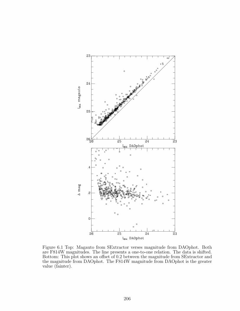
Figure 6.1 Top: Magauto from SExtractor verses magnitude from DAOphot. Bothare F814W magnitudes. The line presents a one-to-one relation. The data is shifted.Bottom: This plot shows an offset of 0.2 between the magnitude from SExtractor andthe magnitude from DAOphot. The F814W magnitude from DAOphot is the greatervalue (fainter).
206
between r625 and I814 being both filters on the red end of the spectrum. Bimodality
is observed in Figure 6.3 which shows number of GC candidates verses g475-I814 but
not in r625-I814 . Therefore, the statement in the globular cluster review, Brodie &
Strader (2006), that “no massive elliptical (E) galaxy has been convincingly shown
to lack GC subpopulations” is supported by the system of GCs of ESO325-G004.
The g475-I814 histogram, Figure 6.3, was tested for bimodality using the KMM
(Kaye’s Mixture Modeling) algorithm which compares data to discern if it can be
best described by a single or double Gaussian (Ashman et al. 1994). This also was
mentioned in the NGC1533 study in Chapter 2. The algorithm found the g475-I814
color data to be best described by a double Gaussian with > 99% confidence. It gave
values for the two color peaks, 1.489 and 1.785 mag. We will call the 1.489 mag peak,
the blue peak and the 1.785 mag peak, the red peak. When looking at Figure 6.3,
a minimum at ∼ 1.7 can be seen. This figure binned the number of GCs in g475-I814
magnitude intervals of 0.05. The file that created Figure 6.3 had the lowest number
of GCs in the 1.70 color bin. Binning the data by smaller g475-I814 intervals such as
0.01 and 0.025, we found that the bin with the lowest number of GCs was still 1.70.
Therefore, g475-I814 = 1.70 is taken to be the minimum between the blue and red peak
and the color data was split between blue and red using this value. The blue GCs are
candidates with 1.30 ≤ g475-I814 < 1.70 and the red GCs are candidates with 1.70 ≤g475-I814 ≤ 2.00. KMM claims the blue population is 59.2% and the red population
is 40.8% of the total detected GC population, 405, in ESO325-G004. However, when
the data file is split into two catalogs, using 1.70 as the dividing value, the numbers
are actually 274 blue GCs (67.7%) and 131 red GCs (32.3%).
6.3 Distribution
The Milky Way GC subpopulations, briefly mentioned in section 1.7.1, do tend
to depend on the radius from the galactic center (galactic radius), with the “Halo”
containing more metal-poor, blue GCs and the disk and bulge corresponding to more
metal-rich, red GCs (Zinn 1985; Cote 1999) . Even though the Milky Way is a spiral
207
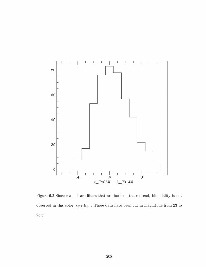
Figure 6.2 Since r and I are filters that are both on the red end, bimodality is not
observed in this color, r625-I814 . These data have been cut in magnitude from 23 to
25.5.
208

Figure 6.3 Bimodality is seen in this magnitude verse g475-I814 plot. These data have
been cut in magnitude from 23 to 25.5.
209

Figure 6.4 Distribution of ESO325-G004 GC subpopulations in pixel space (20
pix/arcsec)
and our study contains only ellipticals, it might be interesting to plot the two GC
subpopulations of ESO325-G004 to see if there is any correlation between color and
galactic radius. Figure 6.4 represents the blue and red subpopulations plotted with
their x,y coordinates in pixels. The blue GCs are plotted with blue points and the
red GCs are plotted with red. This Figure seems to show a concentration of red GC
candidates near the center of ESO325-G004. To further verify that this is the case,
Figure 6.5 shows the number density of GC’s for the blue (bottom plot) and red (top
plot) subpopulations verses galactic radius.
In section 5.2.2, the log-log plots of number density verses mean binned radius
210

Figure 6.5 The top plot is number of Blue GCs per area verses radius from ESO325-
G004 center in pixels. The bottom plot is the same plot but with Red GCs.
211
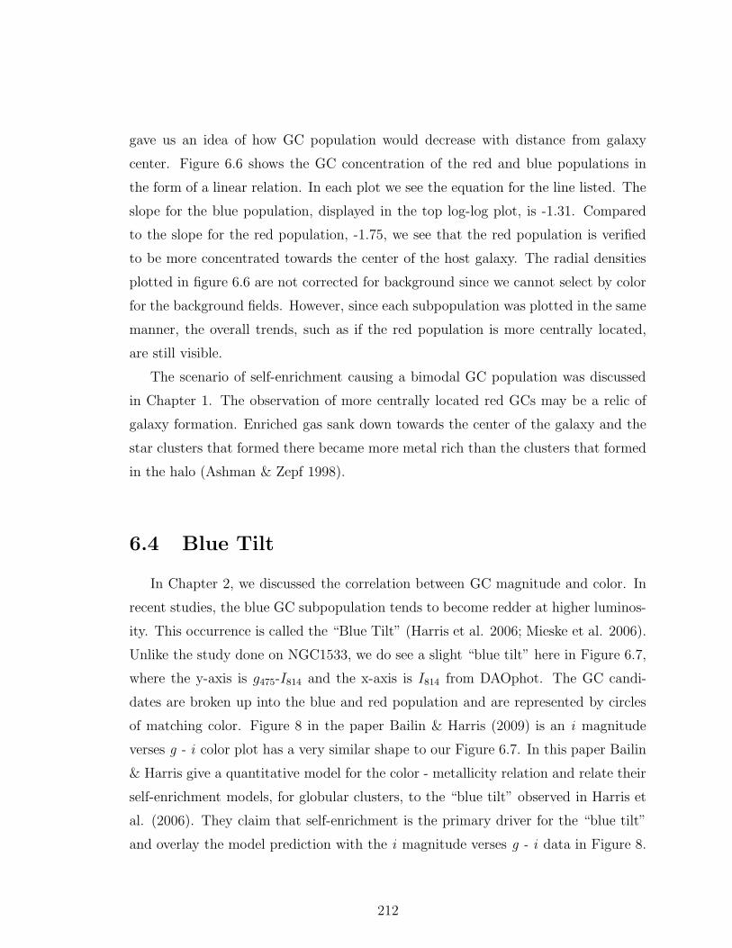
gave us an idea of how GC population would decrease with distance from galaxy
center. Figure 6.6 shows the GC concentration of the red and blue populations in
the form of a linear relation. In each plot we see the equation for the line listed. The
slope for the blue population, displayed in the top log-log plot, is -1.31. Compared
to the slope for the red population, -1.75, we see that the red population is verified
to be more concentrated towards the center of the host galaxy. The radial densities
plotted in figure 6.6 are not corrected for background since we cannot select by color
for the background fields. However, since each subpopulation was plotted in the same
manner, the overall trends, such as if the red population is more centrally located,
are still visible.
The scenario of self-enrichment causing a bimodal GC population was discussed
in Chapter 1. The observation of more centrally located red GCs may be a relic of
galaxy formation. Enriched gas sank down towards the center of the galaxy and the
star clusters that formed there became more metal rich than the clusters that formed
in the halo (Ashman & Zepf 1998).
6.4 Blue Tilt
In Chapter 2, we discussed the correlation between GC magnitude and color. In
recent studies, the blue GC subpopulation tends to become redder at higher luminos-
ity. This occurrence is called the “Blue Tilt” (Harris et al. 2006; Mieske et al. 2006).
Unlike the study done on NGC1533, we do see a slight “blue tilt” here in Figure 6.7,
where the y-axis is g475-I814 and the x-axis is I814 from DAOphot. The GC candi-
dates are broken up into the blue and red population and are represented by circles
of matching color. Figure 8 in the paper Bailin & Harris (2009) is an i magnitude
verses g - i color plot has a very similar shape to our Figure 6.7. In this paper Bailin
& Harris give a quantitative model for the color - metallicity relation and relate their
self-enrichment models, for globular clusters, to the “blue tilt” observed in Harris et
al. (2006). They claim that self-enrichment is the primary driver for the “blue tilt”
and overlay the model prediction with the i magnitude verses g - i data in Figure 8.
212
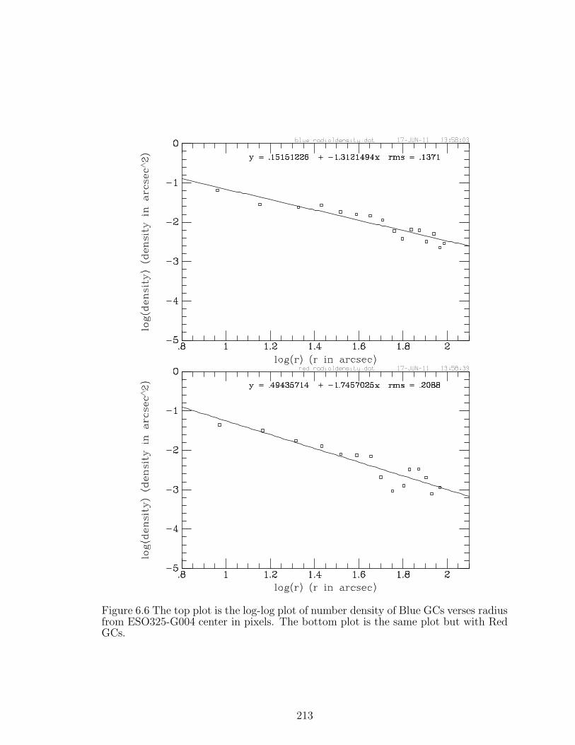
Figure 6.6 The top plot is the log-log plot of number density of Blue GCs verses radiusfrom ESO325-G004 center in pixels. The bottom plot is the same plot but with RedGCs.
213

It shows a curve, that contains the GC candidates, which is fairly flat starting from
24 magnitude and climbing steeper towards brighter magnitudes (< 24) ending at the
red peak vertical line in g - i. The blue GCs in Figure 6.7 seem consistent with this
curve. Harris et al. (2006) claims that for very bright galaxies the GC population
starts to become less obviously bimodal at MI < −10.5. In our study this MI value
corresponds to an I814 of 25.3. Since Figure 6.7 is subject to a color cut, it is hard to
confirm that our slight “blue tilt” starts around 25.3 mag.
This suggests that the slight “blue tilt” here is due to self-enrichment, which
Bailin & Harris (2009) claim only creates the “blue tilt” at masses of 106 M�. This is
the reason evidence of the “blue tilt” comes from GCs in bright ellipticals in galaxy
groups or clusters. ESO325-G004 seems to meet these requirements. Harris et al.
(2006) mentions that the blue and red peaks merge into a single broad peak but since
there are only about 15 objects brighter than 24 mag, it is difficult to make verify in
our data set. Also, as discussed in chapter 2, if the “tilt” is due to mergers, it may
only be a stronger occurrence that accompanies richer systems. If the galaxy is in a
poor cluster, as is ESO325-G004, it would be another reason why a “tilt” is slight.
The “blue tilt” has been detected by Peng et al. (2009) and Harris et al. (2009).
If the assumption is made that blue candidates are metal-poor, as stated in chapter 2
and Blakeslee et al. (2010), the simplest explanation for the “tilt” is self-enrichment,
where the most massive metal-poor GCs were able to keep a small portion of self-
enriched gas while star formation continues. However, the quick relation between
color and metallicity of a globular cluster, which is so often used in studies involving
bimodal color GC distributions, is under investigation (Yoon et al. 2006; Cantiello
& Blakeslee 2007; Blakeslee et al. 2010) to see if this simple assumption that blue
equals metal poor and red equals metal rich is reasonable.
6.5 Metallicity-Color Relation
A common occurrence of bimodality in the color distributions of GC popula-
tions can be perceived to be a reflection of metallicity (see Chapter 1, section 1.7.1)
214
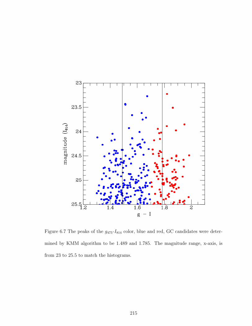
Figure 6.7 The peaks of the g475-I814 color, blue and red, GC candidates were deter-
mined by KMM algorithm to be 1.489 and 1.785. The magnitude range, x-axis, is
from 23 to 25.5 to match the histograms.
215
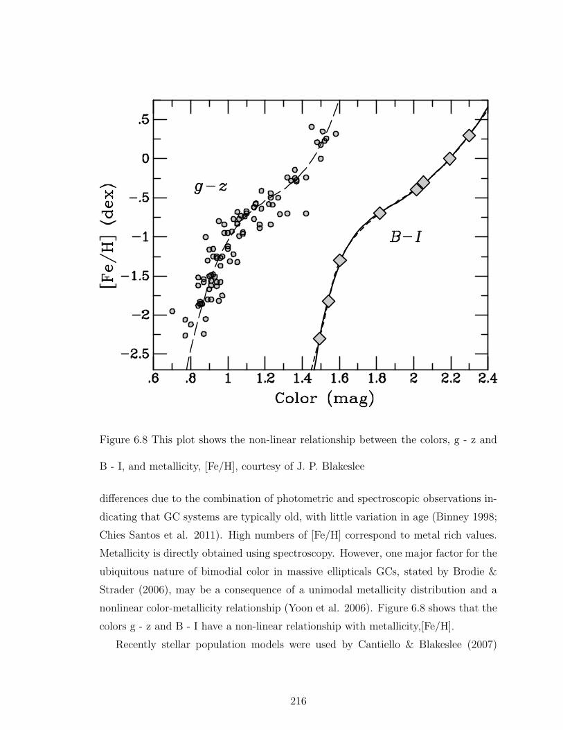
Figure 6.8 This plot shows the non-linear relationship between the colors, g - z and
B - I, and metallicity, [Fe/H], courtesy of J. P. Blakeslee
differences due to the combination of photometric and spectroscopic observations in-
dicating that GC systems are typically old, with little variation in age (Binney 1998;
Chies Santos et al. 2011). High numbers of [Fe/H] correspond to metal rich values.
Metallicity is directly obtained using spectroscopy. However, one major factor for the
ubiquitous nature of bimodial color in massive ellipticals GCs, stated by Brodie &
Strader (2006), may be a consequence of a unimodal metallicity distribution and a
nonlinear color-metallicity relationship (Yoon et al. 2006). Figure 6.8 shows that the
colors g - z and B - I have a non-linear relationship with metallicity,[Fe/H].
Recently stellar population models were used by Cantiello & Blakeslee (2007)
216
and Blakeslee et al. (2010) to see if they could reproduce color bimodality and
the “blue tilt”, mentioned in section 6.4, using a stellar population with a unimodal
metallicity distribution. Cantiello & Blakeslee (2007) looked at the color distribution:
B-V, V-R, V-I, B-I, U-R, V-K, J-H, J-K, and H-K and found that “a unimodal
metallicity distribution can be projected into a bimodal color distribution in almost
any of the colors considered here, depending on the properties of the metallicity
distribution, on the particular color index, and on the photometric uncertainty of the
sample.” Figure 6.9 shows the bimodality created using different unimodal metallicity
populations in the color g - z. Each colored curve represents varying metallicities.
The redder curves are more metal rich and the bluer curves are more metal poor.
The metallicity to color relations were plotted and some are seen to have quite
nonlinear form (see Figure 6.8), especially in the color V - I. The nonlinear curve that
relates V - I to metallicity could explain the color bimodalty in V - I that is mentioned
in many studies (Brodie & Strader 2006). A similar shape is mentioned in Blakeslee
et al. (2010) for the [Fe/H] verses color plot (Figure 6.8). There is an inflection
point in these plots that can explain the near equality of red and blue populations
in the “blue tilt” situations because the inflection point is roughly equal to the peak
metallicity of the GC population. The “blue tilt” could also be reproduced using a
unimodal metallicity distribution (Blakeslee et al. 2010) and it is “when the peak
metallicity begins to move through the inflection point that the ’blue tilt’ becomes
most pronounced” (Blakeslee et al. 2010).
The more linear the color-metallicity relation, the more likely a bimodal color
distribution points to actual subpopulations in metallicity, examples being colors V-
K and V-H. The Milky Way GC population has been found to truly be bimodal in
metallicity and so the possibility is present that there are subpopulations of GCs
based on one being metal-poor and one being metal-rich. However, the rule that all
massive ellipiticals have bimodal color distributions may not be due to a bimodal
metallicity distribution.
217

Figure 6.9 This plot shows the production of bimodal color, g - z, using unimodal
metallicity GC populations, courtesy of J. P. Blakeslee. The varying colors for each
curve go from red, metal rich, to blue, metal poor.
218

6.6 Conclusion
We analyzed the galaxy ESO325-G004 using images taken in filters, F475W,
F625W and F814W. They were first run through the object detection program SEx-
tractor and the F814W image was also studied using the object detection program
DAOphot. The two catalogs were merged and then subjected to selection in I814 mag-
nitude, g475-I814 and r625-I814 colors. This new catalog was then tested with KMM
to detect bimodality in the color g475-I814 . KMM indicated that the GC population
was bimodal in the color g475-I814 and gave a blue peak at the value 1.489 and a red
peak at 1.785. The separation between blue and red GCs is g475-I814 = 1.70 mag.
The distribution of the red and blue subpopulations showed the red GCs tended to
be more concentrated at the galactic center. This may be due to settling of enriched
gas toward the galaxy center during the process of formation. Like other ellipticals
in recent studies, the blue population is greater (274) than the red population (131)
and the red GCs are more concentrated at the center (Ashman & Zepf 1998; Peng et
al. 2006).
The “blue tilt” cannot conclusively be detected in our study but is consistent
with observations. In particular, there are no GCs brighter than I814 = 24 (MI814 ≈−11.8) that have colors bluer than the blue peak of the color distribution. If the
blue tilt is present, it is likely due to an overall mass-metallicity in the GC system.
However, because the metallicity-color relations are not necessarily linear, it is difficult
to interpret how the mean color is changing as a function of GC mass. In fact,
nonlinear color-metallicity relations may also be the reason for the commonality of
bimodal populations in massive ellipticals. Further spectroscopy is needed to verify
if there exists true, distinct metal-poor and metal-rich subpopulations within GC
systems.
A table of all GC candidates’ RA, DEC, I814 magnitude (DAOphot), colors (g475−I814 and r625 − I814) and galactic radius is included in Appendix A.
219
Bibliography
[1] Ashman, K. M., Bird, C. M., & Zepf, S. E. 1994, AJ, 108, 2348
[1] Ashman, K. M., & Zepf, S. E. 1998, Globular cluster systems, New York: Cam-
bridge University Press
[3] Bailin, J., & Harris, W. E. 2009, ApJ, 695, 1082
[4] Bertin, E., & Arnouts, S. 1996, A&AS, 117, 393
[5] Blakeslee, J. P., Cantiello, M., & Peng, E. W. 2010, ApJ, 710, 51
[3] Blakeslee, J. P., & Barber DeGraaff, R. 2008, AJ, 136, 2295
[7] Binney, J., & Merrifield, M. 1998, Galactic astronomy / James Binney and Michael
Merrifield. Princeton, NJ : Princeton University Press, 1998. (Princeton series in
astrophysics) QB857 .B522 1998
[6] Brodie, J. P., & Strader, J. 2006, ARA&A, 44, 193
[7] Cantiello, M., & Blakeslee, J. P. 2007, ApJ, 669, 982
[10] Chies-Santos, A. L., Larsen, S. S., Kuntschner, H., Anders, P., Wehner, E. M.,
Strader, J., Brodie, J. P., & Santos, J. F. C. 2011, A&A, 525, A20
[11] Cote, P. 1999, AJ, 118, 406
[12] Harris, W. E., Whitmore, B. C., Karakla, D., Okon, W., Baum, W. A., Hanes,
D. A., & Kavelaars, J. J. 2006, ApJ, 636, 90
220
[13] Harris, W. E., Kavelaars, J. J., Hanes, D. A., Pritchet, C. J., & Baum, W. A.
2009, AJ, 137, 3314
[14] Mieske, S., et al. 2006, ApJ, 653, 193
[9] Peng, E. W., et al. 2006, ApJ, 639, 95
[16] Peng, E. W., et al. 2009, ApJ, 703, 42
[11] Yoon, S.-J., Yi, S. K., & Lee, Y.-W. 2006, Science, 311, 1129
[18] Zinn, R. 1985, ApJ, 293, 424
221

Chapter 7
Summary and Future Work
7.1 Summary and Results
The main study in this thesis is the survey investigating the globular cluster (GC)
populations of 11 galaxies in the Shapley Supercluster. Due to the simplicity of glob-
ular clusters, the characteristics of these populations can contribute to observations
that constrain galaxy, cluster or GC formation models. The characteristics discussed
are total number, specific frequency, distribution and association with galaxy and
cluster properties.
After an introduction to the history of globular clusters and various terminology
in astronomy, we briefly cover galaxy formation and recent developments in globular
cluster studies. We discuss bimodality in color of GCs surrounding giant ellipticals
and the wide range of values for specific frequency, SN , in this type of galaxy.
We then do a related study on the GC population of the S0 galaxy in the Dorado
Group, NGC1533. NGC1533 was imaged by ACS through F814W and F606W. The
galaxy was found to have a faint spiral structure after model subtraction. NGC1533 is
known to have H II regions with possible star formation far from the galactic center.
We found four H II regions along one of the faint spiral arms. This galaxy seems to
222

be in transition from an Sba to an S0 galaxy. These H II regions and the hint of
transition may be due to interaction between neighboring galaxies. The interaction
between NGC1533 and IC 2038/2039 is documented (Ryan-Weber et al. 2004).
We use the distance indicators described in Chapter 1 to find distance to NGC1533
three different ways. The SBF distance is 19.4 ± 1.1 Mpc. The distance obtained
using the GCLF method was equal to 19.4 Mpc, within errors. Distance to NGC1533
calculated using the median half-light GC radius was 18.6 ± 2.0 Mpc. There seems
to be a correlation between GC size (half-light radius) and distance from NGC1533
(galactocentric radius). We find SN to be 1.3 ± 0.2, which is typical for a S0 galaxy.
The color F606W - F814W was converted to the color V - I to compare NGC1533’s
GC population to other studies. The KMM algorithm indicated that the GC pop-
ulation was bimodal in V - I with peaks at roughly 0.92 and 1.22 mag. There is
no evidence for the “blue tilt” (blue GCs becoming redder at brighter magnitudes).
However, the blue tilt has been more commonly seen in massive ellipticals.
The conclusion that NGC1533 is a galaxy in transition is further supported by
the GC population having similarities in size, color and luminosity, with Virgo early-
type galaxies but also showing a strong dependence of size of GCs with galactocentric
radius like the GCs of the Milky Way (Barber DeGraaff 2007).
Ultra Compact Dwarfs (UCD) are a new classification of stellar system that is
thought to be associated with globular clusters. Their physical size is greater than
GCs (3-5 pcs) but smaller than dwarf galaxies. We searched for UCDs in the giant
elliptical ESO325-G004, using three band imaging (F475W, F814W and F625W).
This galaxy is a member of Abell S0740, a poor cluster in the Shapley Supercluster.
We selected objects that were brighter than 99% of the expected GC population, the
same GC color range at this redshift, shape similar to a GC and half light radii (size)
in the 10-100pc range. Spectra need to be taken to confirm the UCD candidates
found are associated with ESO325-G004. We also included a group of larger compact
galaxies of 100-300pc in our study. When color data for all the UCD candidates was
plotted, the population seemed to be weighted toward the red. There also seemed
to be a bifurcation in UCD candidate size. There seemed to be a group with size
similar to GCs and then another clump greater than 40pc. These two distinct groups
223
may point to two different mechanisms in creating UCDs. Some propose that UCDs
are just tidally stripped dwarf galaxies. We found that most of the UCD candidates
had visible surrounding halo light, which is consistent with galaxy threshing models.
Other studies suggest that UCDs are just a high luminosity extension of the GC
system. A combination of both views may be closer to reality (Blakeslee & Barber
DeGraaff 2008).
The GC populations of the 11 galaxies in the Shapley Supercluster were then
studied, using imaging from ACS in F814W. Data reduction was done using the
detection software DAOphot and described in Chapter 4 along with a brief description
of the Shapley Supercluster. We were interested in obtaining total number of GCs,
distribution, and specific frequencies (SNs). To obtain the total number of the 11
GC systems, we needed to take into account many corrections. The number of GCs
detected for each of the 11 galaxies was not a reflection of the actual GC population
due to completeness in detection, background and foreground objects in the field,
the magnitude range imposed in the selection and the radial limits imposed by our
selection and HST/ACS. Another correction needed to be considered when counting
the number of GCs associated with members of Abell 3558. Because the BCG,
ESO444-G046, was massive and centrally located, we considered how much it’s GC
population “contaminated” the neighboring members.
Once all these corrections were obtained a total number of GCs, Ntot could be
estimated for each of the 11 galaxies in the survey. The Ntot values ranged from ∼850 to 27,500. Plotting a log-log plot of Ntot verses LV , luminosity of the galaxy in
the V band, showed a relation of,
Ntot ∝ L1.6V (7.1)
where the power of 1.6 is contrary to the once believed value of 1.0. This result
suggests that the formation of the GC population must be dependent on something
other than simply the host galaxy’s star formation history.
The SN values ranged from values as low as 1.47 (similar to NGC1533) to values as
high as 10.3. Note that these are the specific frequencies estimated within a radius of
224

100 kpc; the GC populations of the largest galaxies likely extend beyond this radius,
so the actual SN values for these largest galaxies could be significantly higher. We
find a strong correlation of SN with the dynamical mass of the galaxy.
The lowest specific frequency value of 1.47 and the two highest values of 10.3 and
8.1 seem to not only relate to the size of the galaxy but also to the location of the
galaxy in the host cluster. Additionally the reason for two galaxies, with drastically
different sizes, having the same SN values may be due to the bigger galaxy’s great
distance from its cluster center. This result points toward GC populations being
associated with the host cluster as well as the host galaxy.
Stronger evidence comes in the form of the concept of Intracluster Globular Clus-
ters (IGCs), which are thought to be GCs associated with the cluster’s potential well.
Figure 5.27 strongly suggests that four of the five Abell clusters contain IGCs. The
IGC population may increase the GC population of centrally located cluster mem-
bers, which makes sense when thinking of ESO383-G076 and ESO444-G046. Their
large numbers of GCs may just be the addition of IGCs because ESO383-G076 and
ESO444-G046 are both within 1 arcmin of the cluster center.
The additional imaging of ESO325-G004, used to search for UCDs, was used to
receive color data for the GC population. The GC population from Chapter 5 was
combined with data obtained in the study done in Chapter 3. The GC candidates were
further selected with g475-I814 and r625-I814 . The KMM algorithm confirmed that the
GC population was bimodal in g475-I814 with a red peak at 1.785 mag and a blue peak
at 1.489 mag. The minimum at 1.70 was used as the dividing value to separate the
data into two populations, a red and a blue. The red population was found to be more
concentrated towards the center of ESO325-G004. The blue population was found to
be more abundant (274 blue, 131 red). The GC color population of ESO325-G004 is
typical of a massive elliptical (Ashman & Zepf 1998; Peng et al. 2006).
The “blue tilt” discussed earlier was present, if only slightly. However, this
phenomenon was produced in models of star clusters with unimodal metallicities
(Blakeslee et al. 2010), so the tilt is not proof that there are really two distinct metal-
licity subpopulations. The bimodality through this color also may be a consequence of
color-metallicity conversions. This concept, of directly correlating bimodality in color
225
to bimodality in metallicity, is discussed in Chapter 6 and first mentioned in Yoon et
al. (2006). Models have been run that create bimodal color distribution using stellar
populations with unimodal metallicity (Cantiello & Blakeslee 2007; Blakeslee et al.
2010). However, the Milky Way does have two populations of GCs that are bimodal
in color and metallicity. This has been verified with spectroscopy. Therefore, it is
possible that some GC populations are bimodal in both color and metallicity but the
common observation that GC populations in ellipticals are bimodal in color (Brodie
& Strader 2006) may not point towards bimodality in metallicity.
7.2 Future Work
Spectra of the UCD candidates in Chapter 3 have been obtained to verify the
candidate’s location and need to be further reduced. I hope to do this work directly
after papers are published with results from this thesis.
Color data would be very helpful in investigating if bimodality is present in the
other 10 galaxies. Second band imaging in F475W (comparable to g) will be available
for ESO444-G046 and ESO509-G008. HST Proposal 12238 has been submitted by
William Harris and accepted for Cycle 18 of HST which ends August 2011. I am a
co-investigator on said proposal (Harris 2009).
One band imaging in F814w using HST/ACS of Abell 1689 was recently completed
(HST Proposal 11710, Blakeslee 2008). It is an extreme GC population. Estimates
for a galaxy of this size is a GC population of ∼ 100,000. At a redshift of z = 0.183,
it would be the biggest, farthest GC population studied to date (Blakeslee 2008). A
total number of GCs would be helpful in testing formation hypotheses. Since I am a
co-investigator on this proposal, I hope to help with this important project.
226

Bibliography
[1] Ashman, K. M., & Zepf, S. E. 1998, Globular cluster systems, New York: Cam-
bridge University Press
[2] Barber DeGraaff, R., Blakeslee, J. P., Meurer, G. R., & Putman, M. E. 2007,
arXiv:0710.0893
[3] Blakeslee, J. P., & Barber DeGraaff, R. 2008, AJ, 136, 2295
[4] Blakeslee, J. 2008, HST Proposal, 11710
[5] Blakeslee, J. P., Cantiello, M., & Peng, E. W. 2010, ApJ, 710, 51
[6] Brodie, J. P., & Strader, J. 2006, ARA&A, 44, 193
[7] Cantiello, M., & Blakeslee, J. P. 2007, ApJ, 669, 982
[8] Harris, W. 2009, HST Proposal, 12238
[9] Peng, E. W., et al. 2006, ApJ, 639, 95
[10] Ryan-Weber, E. V., et al. 2004, AJ, 127, 1431
[11] Yoon, S.-J., Yi, S. K., & Lee, Y.-W. 2006, Science, 311, 1129
227
Appendix A
ESO325-G004 GCs
This table contains the id, RA, Dec, I band apparent magnitude, colors in g - I
and r - I and radius from center of host galaxy in pixels. This data list was created
by combining detections from the software DAOphot and SExtractor.
228
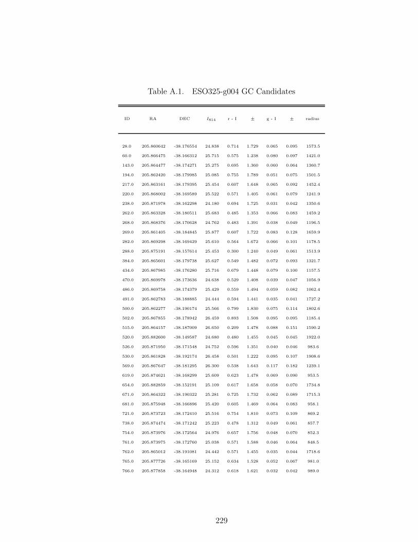
Table A.1. ESO325-g004 GC Candidates
ID RA DEC I814 r - I ± g - I ± radius
28.0 205.860642 -38.176554 24.838 0.714 1.729 0.065 0.095 1573.5
60.0 205.866475 -38.166312 25.715 0.575 1.238 0.080 0.097 1421.0
143.0 205.864477 -38.174271 25.275 0.695 1.360 0.060 0.064 1360.7
194.0 205.862420 -38.179985 25.085 0.755 1.789 0.051 0.075 1501.5
217.0 205.863161 -38.179395 25.454 0.607 1.648 0.065 0.092 1452.4
220.0 205.868002 -38.169589 25.522 0.571 1.405 0.061 0.079 1241.9
238.0 205.871978 -38.162298 24.180 0.694 1.725 0.031 0.042 1350.6
262.0 205.863328 -38.180511 25.683 0.485 1.353 0.066 0.083 1459.2
268.0 205.868376 -38.170628 24.762 0.483 1.391 0.038 0.049 1196.5
269.0 205.861405 -38.184845 25.877 0.607 1.722 0.083 0.128 1659.9
282.0 205.869298 -38.169429 25.610 0.564 1.672 0.066 0.101 1178.5
288.0 205.875191 -38.157614 25.453 0.300 1.240 0.049 0.061 1513.9
384.0 205.865601 -38.179738 25.627 0.549 1.482 0.072 0.093 1321.7
434.0 205.867985 -38.176280 25.716 0.679 1.448 0.079 0.100 1157.5
470.0 205.869978 -38.173636 24.638 0.529 1.408 0.039 0.047 1056.9
486.0 205.869758 -38.174379 25.429 0.559 1.494 0.059 0.082 1062.4
491.0 205.862783 -38.188885 24.444 0.594 1.441 0.035 0.041 1727.2
500.0 205.862277 -38.190174 25.566 0.799 1.830 0.075 0.114 1802.6
502.0 205.867855 -38.178942 26.459 0.893 1.508 0.095 0.095 1185.4
515.0 205.864157 -38.187009 26.650 0.209 1.478 0.088 0.151 1590.2
520.0 205.882600 -38.149587 24.680 0.480 1.455 0.045 0.045 1922.0
526.0 205.871950 -38.171548 24.752 0.596 1.351 0.040 0.046 983.6
530.0 205.861828 -38.192174 26.458 0.501 1.222 0.095 0.107 1908.6
569.0 205.867647 -38.181295 26.300 0.538 1.643 0.117 0.182 1239.1
619.0 205.874621 -38.168299 25.609 0.623 1.478 0.069 0.090 953.5
654.0 205.882859 -38.152191 25.109 0.617 1.658 0.058 0.070 1734.8
671.0 205.864322 -38.190322 25.281 0.725 1.732 0.062 0.089 1715.3
681.0 205.875948 -38.166896 25.420 0.605 1.469 0.064 0.083 958.1
721.0 205.873723 -38.172410 25.516 0.754 1.810 0.073 0.109 869.2
738.0 205.874474 -38.171242 25.223 0.478 1.312 0.049 0.061 857.7
754.0 205.873976 -38.172564 24.976 0.657 1.756 0.048 0.070 852.3
761.0 205.873975 -38.172760 25.038 0.571 1.588 0.046 0.064 848.5
762.0 205.865012 -38.191081 24.442 0.571 1.455 0.035 0.044 1718.6
765.0 205.877726 -38.165169 25.152 0.634 1.528 0.052 0.067 981.0
766.0 205.877858 -38.164948 24.312 0.618 1.621 0.032 0.042 989.0
229

Table A.1 (cont’d)
ID RA DEC I814 r - I ± g - I ± radius
776.0 205.874810 -38.171311 25.454 0.797 1.872 0.074 0.112 838.3
778.0 205.863339 -38.194702 25.220 0.602 1.587 0.053 0.073 1962.7
788.0 205.868578 -38.186931 24.953 0.611 1.631 0.050 0.068 1376.6
810.0 205.868411 -38.185071 25.209 0.680 1.601 0.058 0.074 1312.1
835.0 205.867649 -38.187895 24.597 0.765 1.824 0.046 0.066 1459.9
837.0 205.867762 -38.187681 25.506 1.044 1.718 0.089 0.097 1445.7
850.0 205.886633 -38.148787 25.449 0.536 1.439 0.075 0.076 1953.7
874.0 205.872874 -38.177420 24.674 0.605 1.472 0.042 0.052 887.4
888.0 205.871105 -38.181362 25.159 0.485 1.417 0.050 0.062 1056.9
890.0 205.869245 -38.185189 25.830 0.549 1.413 0.069 0.088 1276.0
895.0 205.874678 -38.174252 25.131 0.633 1.471 0.053 0.065 787.2
899.0 205.875298 -38.173206 23.225 0.690 1.820 0.022 0.029 767.9
900.0 205.875419 -38.173210 25.485 0.589 1.464 0.060 0.074 761.2
938.0 205.865496 -38.194187 24.008 0.641 1.617 0.029 0.038 1849.7
965.0 205.885538 -38.153930 24.715 0.674 1.741 0.044 0.060 1589.1
973.0 205.872986 -38.179690 25.689 0.528 1.369 0.079 0.090 916.1
974.0 205.884595 -38.156084 26.578 0.684 1.478 0.113 0.142 1442.0
1020.0 205.885471 -38.155084 25.739 0.719 1.614 0.081 0.111 1507.0
1049.0 205.877138 -38.172656 24.801 0.501 1.395 0.041 0.050 680.1
1055.0 205.871939 -38.183268 25.102 0.555 1.547 0.050 0.067 1074.1
1079.0 205.876105 -38.175246 25.063 0.741 1.786 0.057 0.077 699.1
1093.0 205.869380 -38.189388 24.745 0.589 1.495 0.040 0.053 1451.9
1097.0 205.868514 -38.191156 25.524 0.520 1.464 0.062 0.084 1574.7
1101.0 205.872392 -38.183365 25.398 0.546 1.652 0.058 0.088 1055.5
1106.0 205.885299 -38.157121 25.291 0.521 1.484 0.052 0.070 1362.5
1109.0 205.877614 -38.172840 25.526 0.524 1.450 0.062 0.084 650.2
1118.0 205.869887 -38.189896 25.857 0.642 1.810 0.077 0.128 1455.6
1121.0 205.874963 -38.178758 24.265 0.596 1.550 0.032 0.040 789.9
1127.0 205.876625 -38.175445 25.677 0.696 1.746 0.079 0.118 669.2
1131.0 205.879665 -38.169320 23.443 0.595 1.512 0.022 0.026 685.2
1135.0 205.888019 -38.152373 24.549 0.721 1.855 0.051 0.058 1693.0
1140.0 205.874940 -38.179069 24.510 0.762 1.889 0.041 0.062 797.2
1142.0 205.875634 -38.177639 24.828 0.601 1.422 0.045 0.052 735.1
1152.0 205.874670 -38.179760 25.133 0.667 1.708 0.064 0.080 827.4
1154.0 205.870054 -38.189302 25.638 0.622 1.687 0.072 0.105 1419.5
230

Table A.1 (cont’d)
ID RA DEC I814 r - I ± g - I ± radius
1168.0 205.880585 -38.168193 24.595 0.488 1.399 0.038 0.047 709.7
1169.0 205.880898 -38.167352 25.373 0.484 1.401 0.057 0.071 747.7
1202.0 205.884740 -38.160045 24.899 0.630 1.673 0.044 0.063 1159.4
1211.0 205.871117 -38.188197 23.271 0.602 1.674 0.021 0.026 1321.5
1230.0 205.883558 -38.163223 25.330 0.473 1.407 0.053 0.070 952.4
1244.0 205.874585 -38.181593 25.687 0.551 1.410 0.080 0.090 884.8
1250.0 205.878824 -38.173071 25.446 0.616 1.939 0.067 0.117 580.1
1260.0 205.870901 -38.189530 24.471 0.520 1.425 0.034 0.042 1396.3
1262.0 205.871379 -38.188618 23.944 0.671 1.752 0.029 0.038 1331.2
1272.0 205.874445 -38.182516 25.553 0.665 1.900 0.070 0.119 924.4
1290.0 205.879516 -38.172453 24.451 0.502 1.392 0.034 0.041 561.8
1307.0 205.884431 -38.162813 24.935 0.757 1.883 0.049 0.077 967.9
1336.0 205.884454 -38.163379 25.601 0.703 1.871 0.072 0.120 928.0
1341.0 205.878136 -38.176398 24.677 0.672 1.744 0.042 0.059 583.8
1360.0 205.880472 -38.172092 25.353 0.536 1.451 0.059 0.073 526.6
1369.0 205.878073 -38.177114 25.632 0.533 1.458 0.069 0.088 592.8
1381.0 205.878530 -38.176650 25.079 0.752 1.881 0.059 0.088 563.1
1392.0 205.878519 -38.176908 25.151 0.715 1.869 0.060 0.094 565.7
1406.0 205.879198 -38.175896 24.964 0.727 1.860 0.053 0.078 522.5
1408.0 205.875311 -38.183856 24.826 0.745 1.860 0.048 0.070 938.5
1419.0 205.878146 -38.178253 25.344 0.474 1.392 0.058 0.071 606.5
1423.0 205.880592 -38.173308 25.523 0.698 1.733 0.073 0.107 480.8
1425.0 205.880902 -38.172718 25.657 0.489 1.618 0.069 0.104 483.1
1430.0 205.877879 -38.179017 24.846 0.647 1.631 0.048 0.061 638.5
1431.0 205.878875 -38.176978 25.146 0.636 1.617 0.058 0.075 546.6
1436.0 205.879446 -38.175922 25.061 0.592 1.588 0.054 0.071 508.5
1439.0 205.880350 -38.174126 25.162 0.532 1.351 0.054 0.063 474.5
1454.0 205.875859 -38.183540 24.633 0.496 1.480 0.039 0.051 899.8
1462.0 205.878033 -38.179299 25.578 0.612 1.457 0.074 0.090 637.7
1468.0 205.880818 -38.173701 24.556 0.780 1.787 0.045 0.059 458.6
1474.0 205.882297 -38.170771 25.250 0.688 1.634 0.062 0.081 505.9
1488.0 205.881464 -38.172738 25.480 0.699 1.539 0.072 0.087 454.6
1501.0 205.878516 -38.179115 25.056 0.682 1.545 0.056 0.067 607.4
1503.0 205.880189 -38.175799 24.584 0.578 1.441 0.041 0.048 466.5
1512.0 205.879948 -38.176494 25.726 0.540 1.604 0.081 0.112 482.1
231

Table A.1 (cont’d)
ID RA DEC I814 r - I ± g - I ± radius
1518.0 205.880748 -38.175037 25.153 0.770 1.906 0.066 0.098 439.0
1521.0 205.877692 -38.181316 25.083 0.589 1.460 0.056 0.062 722.8
1522.0 205.877771 -38.181370 25.318 0.634 1.631 0.066 0.084 721.1
1537.0 205.880583 -38.175754 24.992 0.648 1.817 0.052 0.078 444.3
1540.0 205.881337 -38.174266 24.741 0.641 1.649 0.046 0.060 418.0
1548.0 205.880318 -38.176435 24.607 0.553 1.502 0.040 0.049 460.8
1564.0 205.889992 -38.156971 25.472 0.516 1.440 0.059 0.077 1364.6
1567.0 205.874512 -38.188595 24.785 0.777 1.875 0.048 0.074 1207.5
1569.0 205.877210 -38.183156 24.562 0.556 1.478 0.037 0.046 823.1
1571.0 205.881514 -38.174459 25.043 0.745 1.704 0.059 0.075 404.6
1581.0 205.894087 -38.149067 25.106 0.597 1.317 0.065 0.056 1957.2
1601.0 205.877051 -38.184249 25.302 0.692 1.776 0.062 0.092 881.8
1606.0 205.884784 -38.168625 25.272 0.533 1.523 0.056 0.076 561.8
1607.0 205.885766 -38.167120 25.966 0.662 1.901 0.095 0.163 648.9
1613.0 205.880538 -38.177399 25.651 0.680 1.478 0.069 0.081 459.9
1634.0 205.882171 -38.174452 25.423 0.803 1.949 0.079 0.121 368.9
1638.0 205.888717 -38.161144 25.107 0.481 1.525 0.046 0.066 1061.4
1643.0 205.882121 -38.174694 24.921 0.598 1.658 0.051 0.070 367.2
1648.0 205.888230 -38.162357 25.839 0.704 1.369 0.074 0.079 974.0
1660.0 205.886279 -38.166494 25.423 0.729 1.623 0.068 0.086 686.9
1664.0 205.884342 -38.170505 25.390 0.646 1.614 0.067 0.089 451.2
1674.0 205.881537 -38.176497 24.685 0.712 1.794 0.049 0.067 392.6
1683.0 205.884799 -38.170031 23.431 0.552 1.511 0.023 0.028 468.8
1684.0 205.886196 -38.167121 25.045 0.642 1.598 0.050 0.066 643.5
1694.0 205.881633 -38.176599 24.401 0.592 1.582 0.038 0.048 388.1
1696.0 205.877732 -38.184567 24.500 0.731 1.761 0.040 0.054 870.4
1746.0 205.883153 -38.174474 25.494 0.582 1.947 0.077 0.132 315.5
1748.0 205.877034 -38.187045 24.165 0.574 1.433 0.030 0.036 1030.6
1786.0 205.878415 -38.185054 25.623 0.528 1.557 0.068 0.095 870.3
1803.0 205.883529 -38.175090 25.710 0.698 1.695 0.097 0.125 283.1
1815.0 205.882929 -38.176593 24.917 0.464 1.369 0.051 0.060 315.5
1821.0 205.874356 -38.194195 25.621 0.646 1.907 0.077 0.132 1540.5
1826.0 205.889276 -38.163971 24.271 0.506 1.343 0.031 0.036 859.0
1830.0 205.879954 -38.182930 25.694 0.583 1.498 0.083 0.099 698.3
1833.0 205.885606 -38.171483 24.755 0.635 1.751 0.045 0.066 354.9
232
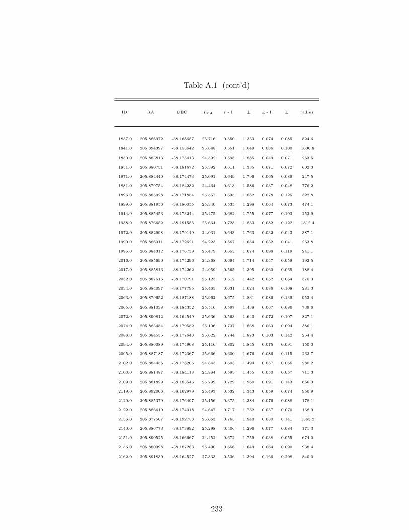
Table A.1 (cont’d)
ID RA DEC I814 r - I ± g - I ± radius
1837.0 205.886972 -38.168687 25.716 0.550 1.333 0.074 0.085 524.6
1841.0 205.894397 -38.153642 25.648 0.551 1.649 0.086 0.100 1636.8
1850.0 205.883813 -38.175413 24.592 0.595 1.885 0.049 0.071 263.5
1851.0 205.880751 -38.181672 25.392 0.611 1.335 0.071 0.072 602.3
1871.0 205.884440 -38.174473 25.091 0.649 1.796 0.065 0.089 247.5
1881.0 205.879754 -38.184232 24.464 0.613 1.586 0.037 0.048 776.2
1896.0 205.885928 -38.171854 25.557 0.635 1.882 0.078 0.125 322.8
1899.0 205.881956 -38.180055 25.340 0.535 1.298 0.064 0.073 474.1
1914.0 205.885453 -38.173244 25.475 0.682 1.755 0.077 0.103 253.9
1938.0 205.876652 -38.191585 25.664 0.728 1.833 0.082 0.122 1312.4
1972.0 205.882998 -38.179149 24.031 0.643 1.763 0.032 0.043 387.1
1990.0 205.886311 -38.172621 24.223 0.567 1.654 0.032 0.041 263.8
1995.0 205.884312 -38.176739 25.479 0.653 1.674 0.098 0.119 241.1
2016.0 205.885690 -38.174296 24.368 0.694 1.714 0.047 0.058 192.5
2017.0 205.885816 -38.174262 24.959 0.565 1.395 0.060 0.065 188.4
2032.0 205.887516 -38.170791 25.123 0.512 1.442 0.052 0.064 370.3
2034.0 205.884097 -38.177795 25.465 0.631 1.624 0.086 0.108 281.3
2063.0 205.879652 -38.187188 25.962 0.675 1.831 0.086 0.139 953.4
2065.0 205.881038 -38.184352 25.516 0.597 1.438 0.067 0.086 739.6
2072.0 205.890812 -38.164549 25.636 0.563 1.640 0.072 0.107 827.1
2074.0 205.883454 -38.179552 25.106 0.737 1.868 0.063 0.094 386.1
2088.0 205.884535 -38.177648 25.622 0.744 1.873 0.103 0.142 254.4
2094.0 205.886089 -38.174908 25.116 0.802 1.845 0.075 0.091 150.0
2095.0 205.887187 -38.172367 25.666 0.600 1.676 0.086 0.115 262.7
2102.0 205.884455 -38.178205 24.843 0.603 1.494 0.057 0.066 280.2
2103.0 205.881487 -38.184118 24.884 0.593 1.455 0.050 0.057 711.3
2109.0 205.881829 -38.183545 25.799 0.729 1.960 0.091 0.143 666.3
2119.0 205.892006 -38.162979 25.493 0.532 1.343 0.059 0.074 950.9
2120.0 205.885379 -38.176497 25.156 0.375 1.384 0.076 0.088 178.1
2122.0 205.886619 -38.174018 24.647 0.717 1.732 0.057 0.070 168.9
2136.0 205.877507 -38.192758 25.663 0.765 1.940 0.080 0.141 1363.2
2140.0 205.886773 -38.173892 25.298 0.406 1.296 0.077 0.084 171.3
2151.0 205.890525 -38.166667 24.452 0.672 1.759 0.038 0.055 674.0
2156.0 205.880398 -38.187283 25.490 0.656 1.649 0.064 0.090 938.4
2162.0 205.891830 -38.164527 27.333 0.536 1.394 0.166 0.208 840.0
233

Table A.1 (cont’d)
ID RA DEC I814 r - I ± g - I ± radius
2163.0 205.885674 -38.176661 25.372 0.424 1.449 0.072 0.084 165.7
2169.0 205.879781 -38.188807 25.371 0.539 1.292 0.058 0.066 1051.5
2171.0 205.891437 -38.165052 25.621 0.585 1.262 0.070 0.080 798.3
2173.0 205.888472 -38.171118 25.775 0.650 1.413 0.090 0.101 342.9
2178.0 205.890835 -38.166371 25.392 0.477 1.365 0.057 0.071 698.3
2180.0 205.897424 -38.152976 25.412 0.574 1.388 0.083 0.072 1726.2
2206.0 205.887664 -38.173101 24.921 0.511 1.480 0.059 0.068 204.9
2214.0 205.880825 -38.187153 26.129 0.748 1.687 0.106 0.147 918.1
2220.0 205.894088 -38.160198 25.660 0.635 1.640 0.074 0.103 1173.9
2224.0 205.885504 -38.177752 24.990 0.486 1.592 0.060 0.076 213.4
2226.0 205.887077 -38.174513 25.974 0.441 1.340 0.140 0.149 124.5
2227.0 205.881728 -38.185491 24.693 0.543 1.438 0.042 0.048 789.0
2251.0 205.887418 -38.174198 25.118 0.678 1.675 0.085 0.100 134.0
2253.0 205.877457 -38.194695 24.819 0.522 1.440 0.025 0.032 1490.4
2253.0 205.877457 -38.194695 2872.743 0.522 1.440 0.025 0.032 1.8
2254.0 205.888221 -38.172691 24.705 0.659 1.670 0.053 0.066 229.9
2257.0 205.885542 -38.178233 24.359 0.676 1.685 0.045 0.055 235.3
2285.0 205.891226 -38.167040 25.212 0.617 1.609 0.054 0.073 656.0
2294.0 205.881130 -38.187766 24.658 0.587 1.554 0.039 0.052 950.2
2302.0 205.886567 -38.176811 24.492 0.622 1.890 0.073 0.101 124.8
2310.0 205.888872 -38.172283 23.713 0.686 1.665 0.030 0.036 260.4
2312.0 205.883834 -38.182550 25.418 0.730 1.914 0.076 0.114 546.1
2330.0 205.880772 -38.189202 25.333 0.642 1.552 0.062 0.082 1052.4
2338.0 205.889969 -38.170622 24.607 0.578 1.443 0.041 0.050 388.6
2346.0 205.888416 -38.173901 24.018 0.644 1.776 0.039 0.049 142.7
2353.0 205.889646 -38.171515 24.487 0.667 1.984 0.042 0.066 321.9
2356.0 205.888725 -38.173362 25.465 0.431 1.532 0.088 0.109 182.2
2363.0 205.891171 -38.168456 25.687 0.719 1.678 0.081 0.106 556.8
2374.0 205.890324 -38.170375 25.758 0.650 1.552 0.085 0.108 410.8
2388.0 205.881572 -38.188556 24.959 0.828 1.896 0.054 0.082 991.6
2408.0 205.892309 -38.167030 24.870 0.584 1.538 0.044 0.058 674.2
2409.0 205.884536 -38.182860 25.664 0.636 1.382 0.086 0.094 548.7
2414.0 205.888853 -38.174051 25.991 0.486 1.587 0.164 0.206 134.4
2416.0 205.887042 -38.177807 25.052 0.513 1.665 0.088 0.110 159.2
2486.0 205.884131 -38.184804 24.495 0.589 1.514 0.039 0.045 686.9
234
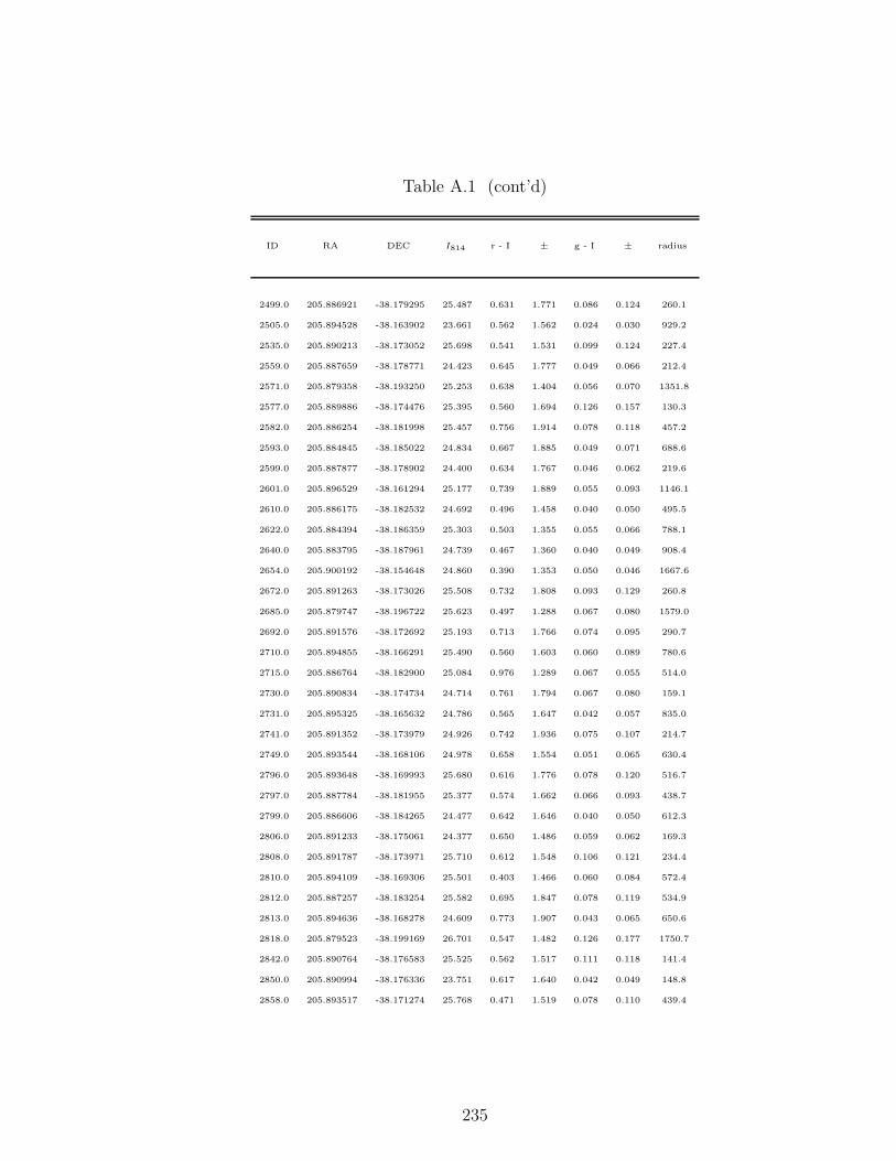
Table A.1 (cont’d)
ID RA DEC I814 r - I ± g - I ± radius
2499.0 205.886921 -38.179295 25.487 0.631 1.771 0.086 0.124 260.1
2505.0 205.894528 -38.163902 23.661 0.562 1.562 0.024 0.030 929.2
2535.0 205.890213 -38.173052 25.698 0.541 1.531 0.099 0.124 227.4
2559.0 205.887659 -38.178771 24.423 0.645 1.777 0.049 0.066 212.4
2571.0 205.879358 -38.193250 25.253 0.638 1.404 0.056 0.070 1351.8
2577.0 205.889886 -38.174476 25.395 0.560 1.694 0.126 0.157 130.3
2582.0 205.886254 -38.181998 25.457 0.756 1.914 0.078 0.118 457.2
2593.0 205.884845 -38.185022 24.834 0.667 1.885 0.049 0.071 688.6
2599.0 205.887877 -38.178902 24.400 0.634 1.767 0.046 0.062 219.6
2601.0 205.896529 -38.161294 25.177 0.739 1.889 0.055 0.093 1146.1
2610.0 205.886175 -38.182532 24.692 0.496 1.458 0.040 0.050 495.5
2622.0 205.884394 -38.186359 25.303 0.503 1.355 0.055 0.066 788.1
2640.0 205.883795 -38.187961 24.739 0.467 1.360 0.040 0.049 908.4
2654.0 205.900192 -38.154648 24.860 0.390 1.353 0.050 0.046 1667.6
2672.0 205.891263 -38.173026 25.508 0.732 1.808 0.093 0.129 260.8
2685.0 205.879747 -38.196722 25.623 0.497 1.288 0.067 0.080 1579.0
2692.0 205.891576 -38.172692 25.193 0.713 1.766 0.074 0.095 290.7
2710.0 205.894855 -38.166291 25.490 0.560 1.603 0.060 0.089 780.6
2715.0 205.886764 -38.182900 25.084 0.976 1.289 0.067 0.055 514.0
2730.0 205.890834 -38.174734 24.714 0.761 1.794 0.067 0.080 159.1
2731.0 205.895325 -38.165632 24.786 0.565 1.647 0.042 0.057 835.0
2741.0 205.891352 -38.173979 24.926 0.742 1.936 0.075 0.107 214.7
2749.0 205.893544 -38.168106 24.978 0.658 1.554 0.051 0.065 630.4
2796.0 205.893648 -38.169993 25.680 0.616 1.776 0.078 0.120 516.7
2797.0 205.887784 -38.181955 25.377 0.574 1.662 0.066 0.093 438.7
2799.0 205.886606 -38.184265 24.477 0.642 1.646 0.040 0.050 612.3
2806.0 205.891233 -38.175061 24.377 0.650 1.486 0.059 0.062 169.3
2808.0 205.891787 -38.173971 25.710 0.612 1.548 0.106 0.121 234.4
2810.0 205.894109 -38.169306 25.501 0.403 1.466 0.060 0.084 572.4
2812.0 205.887257 -38.183254 25.582 0.695 1.847 0.078 0.119 534.9
2813.0 205.894636 -38.168278 24.609 0.773 1.907 0.043 0.065 650.6
2818.0 205.879523 -38.199169 26.701 0.547 1.482 0.126 0.177 1750.7
2842.0 205.890764 -38.176583 25.525 0.562 1.517 0.111 0.118 141.4
2850.0 205.890994 -38.176336 23.751 0.617 1.640 0.042 0.049 148.8
2858.0 205.893517 -38.171274 25.768 0.471 1.519 0.078 0.110 439.4
235

Table A.1 (cont’d)
ID RA DEC I814 r - I ± g - I ± radius
2870.0 205.889972 -38.179520 25.249 0.625 1.772 0.069 0.101 276.1
2873.0 205.890713 -38.177481 25.843 0.596 1.448 0.090 0.105 173.1
2879.0 205.897528 -38.163354 25.235 0.503 1.464 0.050 0.070 1038.7
2891.0 205.891858 -38.175127 24.616 0.761 1.786 0.063 0.078 201.4
2895.0 205.890555 -38.177847 23.977 0.696 1.886 0.038 0.051 185.7
2907.0 205.900549 -38.158025 24.718 0.558 1.945 0.055 0.077 1457.4
2908.0 205.890343 -38.178478 24.866 0.654 1.771 0.059 0.078 216.0
2915.0 205.899609 -38.159741 25.574 0.704 1.932 0.072 0.126 1323.4
2923.0 205.890548 -38.178349 24.987 0.644 1.789 0.063 0.087 214.3
2924.0 205.892146 -38.175075 24.725 0.683 1.749 0.062 0.077 218.2
2930.0 205.890813 -38.177846 25.302 0.646 1.581 0.080 0.097 195.3
2932.0 205.897204 -38.164900 24.965 0.820 1.818 0.054 0.077 933.8
2946.0 205.886053 -38.187895 23.508 0.718 1.863 0.024 0.032 875.3
2948.0 205.890208 -38.179381 25.111 0.526 1.532 0.057 0.071 271.3
2953.0 205.891643 -38.176556 24.818 0.710 1.760 0.068 0.083 188.2
2954.0 205.892694 -38.174469 24.580 0.846 1.942 0.059 0.078 262.0
2962.0 205.891513 -38.177064 24.646 0.520 1.498 0.050 0.059 194.1
2963.0 205.892903 -38.174266 25.369 0.471 1.402 0.070 0.084 278.6
2967.0 205.901966 -38.155952 24.920 0.617 1.745 0.058 0.066 1626.8
2973.0 205.891664 -38.176988 25.709 0.540 1.526 0.102 0.122 199.6
2997.0 205.890222 -38.180289 25.342 0.685 1.834 0.069 0.102 333.1
3000.0 205.890637 -38.179596 24.345 0.595 1.564 0.035 0.044 294.8
3007.0 205.890496 -38.180059 25.590 0.629 1.424 0.068 0.079 323.2
3008.0 205.892241 -38.176495 25.086 0.482 1.451 0.057 0.068 220.4
3015.0 205.892943 -38.175199 25.249 0.657 1.638 0.074 0.095 260.2
3049.0 205.896038 -38.169465 24.824 0.630 1.725 0.046 0.066 631.8
3052.0 205.899274 -38.162875 25.031 0.745 1.822 0.052 0.078 1119.8
3053.0 205.889709 -38.182407 24.934 0.628 1.558 0.050 0.065 475.3
3059.0 205.889941 -38.182021 24.151 0.678 1.768 0.033 0.046 450.3
3063.0 205.899421 -38.162735 25.640 0.569 1.321 0.067 0.080 1132.9
3071.0 205.892573 -38.176798 25.060 0.630 1.664 0.066 0.084 243.6
3094.0 205.890121 -38.182202 24.561 0.574 1.541 0.038 0.050 465.0
3097.0 205.897118 -38.167961 25.349 0.789 1.980 0.070 0.113 753.1
3103.0 205.889636 -38.183364 25.537 0.390 1.511 0.061 0.087 543.0
3123.0 205.884680 -38.193769 23.926 0.580 1.539 0.027 0.035 1305.2
236

Table A.1 (cont’d)
ID RA DEC I814 r - I ± g - I ± radius
3124.0 205.892307 -38.178150 25.156 0.528 1.464 0.060 0.074 273.5
3127.0 205.880686 -38.201981 26.740 0.738 1.330 0.088 0.097 1929.7
3130.0 205.897171 -38.168385 24.280 0.570 1.601 0.033 0.043 732.3
3133.0 205.892979 -38.176921 25.485 0.719 1.865 0.086 0.124 268.2
3140.0 205.896046 -38.170920 23.888 0.688 1.819 0.029 0.041 559.9
3158.0 205.901722 -38.159752 25.518 0.757 1.541 0.077 0.091 1383.9
3171.0 205.893466 -38.176774 25.768 0.434 1.298 0.081 0.095 292.4
3179.0 205.887142 -38.189734 25.093 0.589 1.409 0.050 0.060 1000.0
3182.0 205.896523 -38.170646 24.877 0.593 1.547 0.048 0.061 593.4
3186.0 205.893648 -38.176567 25.477 0.425 1.293 0.066 0.081 299.5
3194.0 205.904190 -38.155235 25.058 0.544 1.695 0.065 0.072 1733.8
3198.0 205.896251 -38.171489 25.142 0.649 1.660 0.058 0.079 544.2
3203.0 205.893906 -38.176299 25.050 0.605 1.841 0.060 0.087 311.3
3204.0 205.895556 -38.172952 25.472 0.573 1.726 0.070 0.106 455.1
3213.0 205.902954 -38.158061 25.521 0.668 1.615 0.091 0.097 1524.0
3215.0 205.896038 -38.172201 24.140 0.539 1.563 0.031 0.042 505.7
3236.0 205.897960 -38.168763 25.678 0.757 1.823 0.081 0.122 744.1
3237.0 205.889176 -38.186692 25.065 0.570 1.498 0.053 0.065 779.4
3245.0 205.892957 -38.179142 25.573 0.497 1.726 0.071 0.109 347.4
3260.0 205.894080 -38.177059 25.329 0.771 1.776 0.077 0.100 330.8
3261.0 205.898023 -38.169047 25.227 0.666 1.856 0.059 0.099 732.9
3283.0 205.893179 -38.179370 25.641 0.640 1.733 0.083 0.127 367.9
3290.0 205.890106 -38.185717 25.349 0.600 1.533 0.065 0.078 714.4
3299.0 205.893516 -38.178908 25.733 0.475 1.626 0.072 0.103 360.7
3303.0 205.894071 -38.177806 25.269 0.580 1.301 0.061 0.067 348.0
3312.0 205.893400 -38.179393 25.101 0.812 1.877 0.064 0.096 378.1
3318.0 205.891416 -38.183509 25.699 0.507 1.491 0.077 0.113 574.5
3323.0 205.894169 -38.178080 24.186 0.531 1.409 0.033 0.038 361.3
3324.0 205.899904 -38.166378 24.686 0.705 1.817 0.042 0.063 943.5
3332.0 205.891332 -38.183910 25.247 0.578 1.480 0.058 0.073 601.0
3343.0 205.888653 -38.189500 25.383 0.615 1.812 0.060 0.103 980.6
3345.0 205.890994 -38.184737 24.754 0.669 1.621 0.046 0.058 653.8
3359.0 205.899417 -38.167897 24.868 0.685 1.787 0.047 0.073 846.9
3363.0 205.892012 -38.183120 25.499 0.630 1.452 0.073 0.089 559.1
3393.0 205.892563 -38.182550 25.667 0.803 1.854 0.089 0.128 534.0
237
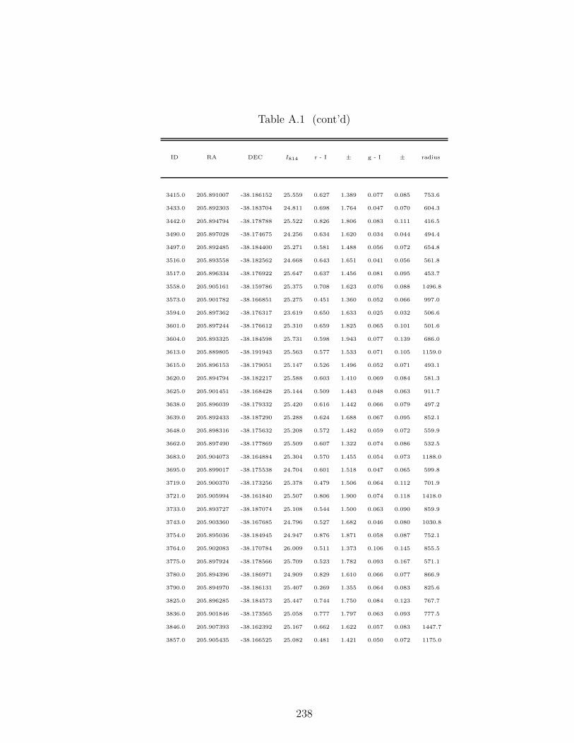
Table A.1 (cont’d)
ID RA DEC I814 r - I ± g - I ± radius
3415.0 205.891007 -38.186152 25.559 0.627 1.389 0.077 0.085 753.6
3433.0 205.892303 -38.183704 24.811 0.698 1.764 0.047 0.070 604.3
3442.0 205.894794 -38.178788 25.522 0.826 1.806 0.083 0.111 416.5
3490.0 205.897028 -38.174675 24.256 0.634 1.620 0.034 0.044 494.4
3497.0 205.892485 -38.184400 25.271 0.581 1.488 0.056 0.072 654.8
3516.0 205.893558 -38.182562 24.668 0.643 1.651 0.041 0.056 561.8
3517.0 205.896334 -38.176922 25.647 0.637 1.456 0.081 0.095 453.7
3558.0 205.905161 -38.159786 25.375 0.708 1.623 0.076 0.088 1496.8
3573.0 205.901782 -38.166851 25.275 0.451 1.360 0.052 0.066 997.0
3594.0 205.897362 -38.176317 23.619 0.650 1.633 0.025 0.032 506.6
3601.0 205.897244 -38.176612 25.310 0.659 1.825 0.065 0.101 501.6
3604.0 205.893325 -38.184598 25.731 0.598 1.943 0.077 0.139 686.0
3613.0 205.889805 -38.191943 25.563 0.577 1.533 0.071 0.105 1159.0
3615.0 205.896153 -38.179051 25.147 0.526 1.496 0.052 0.071 493.1
3620.0 205.894794 -38.182217 25.588 0.603 1.410 0.069 0.084 581.3
3625.0 205.901451 -38.168428 25.144 0.509 1.443 0.048 0.063 911.7
3638.0 205.896039 -38.179332 25.420 0.616 1.442 0.066 0.079 497.2
3639.0 205.892433 -38.187290 25.288 0.624 1.688 0.067 0.095 852.1
3648.0 205.898316 -38.175632 25.208 0.572 1.482 0.059 0.072 559.9
3662.0 205.897490 -38.177869 25.509 0.607 1.322 0.074 0.086 532.5
3683.0 205.904073 -38.164884 25.304 0.570 1.455 0.054 0.073 1188.0
3695.0 205.899017 -38.175538 24.704 0.601 1.518 0.047 0.065 599.8
3719.0 205.900370 -38.173256 25.378 0.479 1.506 0.064 0.112 701.9
3721.0 205.905994 -38.161840 25.507 0.806 1.900 0.074 0.118 1418.0
3733.0 205.893727 -38.187074 25.108 0.544 1.500 0.063 0.090 859.9
3743.0 205.903360 -38.167685 24.796 0.527 1.682 0.046 0.080 1030.8
3754.0 205.895036 -38.184945 24.947 0.876 1.871 0.058 0.087 752.1
3764.0 205.902083 -38.170784 26.009 0.511 1.373 0.106 0.145 855.5
3775.0 205.897924 -38.178566 25.709 0.523 1.782 0.093 0.167 571.1
3780.0 205.894396 -38.186971 24.909 0.829 1.610 0.066 0.077 866.9
3790.0 205.894970 -38.186131 25.407 0.269 1.355 0.064 0.083 825.6
3825.0 205.896285 -38.184573 25.447 0.744 1.750 0.084 0.123 767.7
3836.0 205.901846 -38.173565 25.058 0.777 1.797 0.063 0.093 777.5
3846.0 205.907393 -38.162392 25.167 0.662 1.622 0.057 0.083 1447.7
3857.0 205.905435 -38.166525 25.082 0.481 1.421 0.050 0.072 1175.0
238

Table A.1 (cont’d)
ID RA DEC I814 r - I ± g - I ± radius
3864.0 205.908702 -38.160035 24.390 0.511 1.431 0.050 0.046 1618.4
3894.0 205.904947 -38.168450 25.610 0.869 1.839 0.091 0.137 1077.2
3916.0 205.896466 -38.186385 24.639 0.534 1.495 0.037 0.049 882.5
3937.0 205.911328 -38.156397 25.670 0.589 1.726 0.111 0.122 1910.3
3938.0 205.897354 -38.185021 24.673 0.700 1.825 0.042 0.063 829.6
3939.0 205.897764 -38.184128 25.631 0.631 1.645 0.071 0.103 794.8
3948.0 205.905385 -38.168795 25.353 0.619 1.518 0.066 0.089 1087.0
3956.0 205.902592 -38.174833 25.476 0.561 1.371 0.062 0.074 805.2
3968.0 205.904657 -38.170720 24.875 0.625 1.550 0.045 0.060 991.0
3969.0 205.905041 -38.169924 25.318 0.531 1.491 0.055 0.074 1033.5
3973.0 205.903711 -38.172667 24.518 0.567 1.566 0.036 0.048 895.5
3977.0 205.901394 -38.177493 25.153 0.596 1.642 0.053 0.076 743.0
3983.0 205.904689 -38.171029 25.071 0.475 1.206 0.046 0.055 984.4
3994.0 205.890627 -38.200050 24.987 0.655 1.569 0.049 0.063 1744.5
4014.0 205.909311 -38.162412 24.461 0.697 1.716 0.040 0.052 1529.0
4021.0 205.903189 -38.175078 25.000 0.548 1.506 0.046 0.061 837.5
4028.0 205.909549 -38.162288 25.099 0.490 1.507 0.051 0.066 1545.1
4049.0 205.909414 -38.163117 24.979 0.458 1.339 0.043 0.054 1501.9
4050.0 205.900868 -38.180548 25.702 0.588 1.725 0.077 0.120 780.1
4055.0 205.905000 -38.172223 25.528 0.480 1.379 0.058 0.074 974.1
4056.0 205.905097 -38.172217 24.398 0.576 1.444 0.034 0.044 979.6
4058.0 205.894541 -38.193605 25.398 0.678 1.795 0.063 0.102 1322.2
4092.0 205.894583 -38.194612 25.498 0.479 1.418 0.058 0.080 1392.9
4131.0 205.897396 -38.189355 25.443 0.633 1.550 0.068 0.085 1094.9
4134.0 205.911990 -38.160245 25.159 0.518 1.528 0.065 0.069 1745.4
4138.0 205.907869 -38.168687 25.470 0.560 1.487 0.062 0.085 1216.2
4142.0 205.909127 -38.166255 25.570 0.491 1.336 0.062 0.078 1361.3
4143.0 205.908599 -38.167386 24.916 0.671 1.786 0.047 0.073 1295.3
4153.0 205.902529 -38.180119 25.134 0.497 1.353 0.048 0.059 854.4
4163.0 205.910801 -38.163589 25.532 0.493 1.444 0.058 0.080 1545.0
4182.0 205.904486 -38.177130 24.990 0.773 1.885 0.051 0.082 913.6
4193.0 205.903935 -38.178570 25.402 0.472 1.353 0.051 0.066 898.8
4207.0 205.909626 -38.167452 25.332 0.608 1.442 0.057 0.073 1344.7
4213.0 205.896474 -38.194486 25.650 0.437 1.425 0.065 0.089 1414.8
4215.0 205.893880 -38.199875 25.405 0.599 1.621 0.058 0.086 1754.9
239

Table A.1 (cont’d)
ID RA DEC I814 r - I ± g - I ± radius
4270.0 205.910860 -38.167192 24.329 0.712 1.627 0.035 0.046 1415.5
4289.0 205.904995 -38.180004 24.163 0.627 1.639 0.030 0.041 983.5
4298.0 205.909380 -38.171108 25.675 0.584 1.493 0.073 0.097 1234.7
4307.0 205.914726 -38.160524 25.162 0.539 1.574 0.064 0.069 1854.4
4316.0 205.912062 -38.166399 25.130 0.521 1.405 0.048 0.062 1501.9
4332.0 205.906766 -38.179334 24.376 0.532 1.492 0.034 0.043 1067.3
4373.0 205.914860 -38.162595 25.277 0.554 1.331 0.072 0.063 1775.9
4377.0 205.907785 -38.177118 25.014 0.669 1.609 0.050 0.065 1099.2
4389.0 205.914811 -38.163276 25.458 0.451 1.380 0.065 0.075 1747.6
4433.0 205.910055 -38.174748 25.389 0.341 1.376 0.056 0.076 1226.8
4459.0 205.911713 -38.172504 25.840 0.579 1.645 0.074 0.110 1340.3
4472.0 205.910666 -38.175438 24.136 0.586 1.562 0.029 0.038 1259.0
4550.0 205.912292 -38.176423 25.121 0.697 1.861 0.056 0.091 1351.2
4551.0 205.903048 -38.195670 25.297 0.556 1.485 0.056 0.073 1647.6
4606.0 205.911259 -38.181504 25.085 0.637 1.855 0.051 0.084 1354.1
4643.0 205.903257 -38.200037 25.142 0.703 1.551 0.054 0.070 1931.1
4646.0 205.907500 -38.191457 24.046 0.615 1.417 0.031 0.034 1556.5
4650.0 205.905520 -38.195768 24.119 0.534 1.305 0.029 0.035 1728.0
4653.0 205.907229 -38.192318 24.266 0.579 1.609 0.034 0.044 1591.4
4654.0 205.912951 -38.180713 25.527 0.574 1.617 0.065 0.096 1430.8
4672.0 205.915315 -38.176792 25.245 0.655 1.875 0.058 0.097 1523.2
4673.0 205.913728 -38.178294 25.467 0.462 1.266 0.055 0.068 1442.6
4707.0 205.914877 -38.179244 24.557 0.588 1.445 0.036 0.046 1516.4
4715.0 205.916273 -38.176574 25.282 0.697 1.834 0.060 0.095 1576.8
4745.0 205.920258 -38.169613 25.697 0.499 1.500 0.067 0.096 1857.3
4762.0 205.911233 -38.189002 25.413 0.652 1.512 0.062 0.081 1599.4
4810.0 205.919688 -38.173797 25.145 0.620 1.659 0.048 0.071 1775.7
4831.0 205.920615 -38.172687 25.563 0.607 1.589 0.066 0.094 1836.2
4854.0 205.908150 -38.199458 25.045 0.510 1.270 0.042 0.050 2031.4
4876.0 205.920500 -38.174979 25.211 0.700 1.627 0.055 0.078 1816.4
4939.0 205.913245 -38.192442 25.656 0.621 1.837 0.079 0.124 1842.4
4946.0 205.920150 -38.178620 23.850 0.691 1.949 0.026 0.041 1806.2
5033.0 205.914998 -38.192941 25.562 0.533 1.394 0.065 0.084 1941.6
5048.0 205.921798 -38.179923 24.510 0.564 1.357 0.035 0.042 1911.0
240