Embed Size (px)
Citation preview

A Study of DVB-T2 Standard with
Physical Layer Transceiver Design and
Implementation
Mingchao Yu
July 2011
A thesis submitted for the degree of Master of Philosophy
of the Australian National University


For my parents and grandparents.


Declaration
I hereby declare that the work in this thesis is my own except where otherwise
stated.
Mingchao Yu


Acknowledgements
I would like to dedicate my heartfelt appreciation to my supervisor Parastoo
Sadeghi. It is she who o�ered me the great chance to do research in ANU. She
enlightened my research career with tremendous support, both academically and
�nancially, valuable guidance and in�nite tolerance. Her wisdom and sense of
humor motivated my research, making the dull research full of laugh.
I am indebted to my parents, Yangguang Yu, who convinced me to study
abroad and sponsored me the largest portion of my costs; andWenxia Zhao, whose
thoughtfulness is always with me. I would also appreciate my grandparents, they
always cheer my up when I feel down and try their best to relax my homesickness.
Finally, my grateful thanks to all my friends, both in Australia and China.
They always stay with me and laugh with me. They enriched my everyday life
and prevent me from feeling lonely.
Mingchao Yu
Research School of Engineering, ANU, Canberra
vii

Abstract
The second generation of terrestrial digital video broadcasting (DVB-T2) stan-
dard was published by European Telecommunications Standards Institute in
2008. Compared with the previous DVB-T, the new standard o�ers better ro-
bustness to severe channel conditions and provides up to 60% data capacity in-
crement. These performance improvements are achieved through the adoption of
new channel coding and modulation techniques.
This thesis concentrates on the physical layer transceiver of DVB-T2, includ-
ing bit-interleaved coded modulation (BICM) module, frame mapper module, and
orthogonal-frequency-division-multiplexing (OFDM) modulation module. We es-
tablished a baseband physical layer DVB-T2 system model and thoroughly stud-
ied new techniques included in the transmitter and their receiving methods,
including Bose-Chaudhuri-Hocquenghemand (BCH) codes, low-density parity-
check (LDPC) codes, iterative BICM with rotated constellation, P1 preamble
OFDM symbol, and two OFDM peak-to-average power ratio (PAPR) reduction
techniques. We then proposed some techniques for transceiver optimization. The
main outcomes are:
1. an e�cient BCH encoding/decoding algorithm;
2. a low-complexity iterative demapping and decoding algorithm;
3. novel time domain synchronization and decoding methods for P1 OFDM
symbol;
4. a novel low-complexity time domain channel estimation method for normal
OFDM symbol.
Each transceiver module was �rst implemented and had their performance
evaluated separately. Then they were assembled to investigate the end-to-end bit-
error-rate (BER) performance of the complete baseband physical layer DVB-T2
transceiver. Simulated channel types are additive white Gaussian noise (AWGN)
ix

x
channel, multipath Ricean fading channel, multipath Rayleigh fading channel
and multipath mobile channel. The correctness of our system was con�rmed by
comparing the simulation results with the performance reported in the o�cial
implementation guidelines published by digital video broadcasting (DVB) group.

Contents
Acknowledgements vii
Abstract ix
Notation and Terminology xv
1 Introduction 1
2 System and Channel Models 5
2.1 System Model . . . . . . . . . . . . . . . . . . . . . . . . . . . . . 5
2.1.1 Bit-interleaved Coded Modulation (BICM) . . . . . . . . . 6
2.1.2 Frame Mapper . . . . . . . . . . . . . . . . . . . . . . . . 8
2.1.3 Orthogonal-frequency-division-multiplexing (OFDM) . . . 11
2.2 Channel Models . . . . . . . . . . . . . . . . . . . . . . . . . . . . 12
2.2.1 Additive White Gaussian Noise (AWGN) Channel . . . . . 13
2.2.2 Multipath Rayleigh Fading Channel . . . . . . . . . . . . . 13
2.2.3 Multipath Ricean Fading Channel . . . . . . . . . . . . . . 14
2.2.4 Typical-urban 6-Path (TU-6) Mobile Channel . . . . . . . 15
2.2.5 Uncorrelated Single-path Rayleigh Fading Channel . . . . 15
3 BICM Module 17
3.1 Bose-Chaudhuri-Hocquenghem (BCH) Codes . . . . . . . . . . . . 17
3.1.1 Introduction . . . . . . . . . . . . . . . . . . . . . . . . . . 17
3.1.2 Encoding . . . . . . . . . . . . . . . . . . . . . . . . . . . 18
3.1.3 Decoding . . . . . . . . . . . . . . . . . . . . . . . . . . . 19
3.1.4 Performance Evaluation . . . . . . . . . . . . . . . . . . . 21
3.1.5 Conclusion . . . . . . . . . . . . . . . . . . . . . . . . . . . 26
3.2 Low-density Parity-check (LDPC) Codes . . . . . . . . . . . . . . 26
3.2.1 Introduction . . . . . . . . . . . . . . . . . . . . . . . . . . 26
xi

xii CONTENTS
3.2.2 Encoding . . . . . . . . . . . . . . . . . . . . . . . . . . . 27
3.2.3 Decoding . . . . . . . . . . . . . . . . . . . . . . . . . . . 29
3.2.4 Channel Capacity and Reliability . . . . . . . . . . . . . . 31
3.2.5 Performance over Di�erent Channel Models and Modula-
tion Methods . . . . . . . . . . . . . . . . . . . . . . . . . 33
3.2.6 Conclusion . . . . . . . . . . . . . . . . . . . . . . . . . . . 38
3.3 BICM . . . . . . . . . . . . . . . . . . . . . . . . . . . . . . . . . 38
3.3.1 Introduction . . . . . . . . . . . . . . . . . . . . . . . . . . 38
3.3.2 Bit Interleaver and De-multiplexer . . . . . . . . . . . . . 38
3.3.3 Rotated + Q-Delay Mapping . . . . . . . . . . . . . . . . 41
3.3.4 Iterative Demapping and Decoding . . . . . . . . . . . . . 42
3.3.5 Simulation Results . . . . . . . . . . . . . . . . . . . . . . 46
3.4 Implementation of BICM for P2 OFDM Symbols . . . . . . . . . 48
4 Normal OFDM Symbols 51
4.1 OFDM Overview . . . . . . . . . . . . . . . . . . . . . . . . . . . 51
4.2 Imperfect Receiver . . . . . . . . . . . . . . . . . . . . . . . . . . 52
4.2.1 Timing O�set . . . . . . . . . . . . . . . . . . . . . . . . . 53
4.2.2 Carrier Frequency O�set . . . . . . . . . . . . . . . . . . . 53
4.3 Synchronization . . . . . . . . . . . . . . . . . . . . . . . . . . . . 55
4.3.1 Coarse Timing Synchronization (CTS) . . . . . . . . . . . 56
4.3.2 Fractional Frequency Synchronization (FFS) . . . . . . . . 58
4.3.3 Integer Frequency Synchronization (IFS) . . . . . . . . . . 59
4.3.4 Frame Synchronization . . . . . . . . . . . . . . . . . . . . 60
4.3.5 Fine Timing Synchronization (FTS) . . . . . . . . . . . . . 61
4.4 Channel Estimation . . . . . . . . . . . . . . . . . . . . . . . . . . 63
4.4.1 OFDM Channel Estimation Overview . . . . . . . . . . . . 63
4.4.2 Domain-transform Least-squares Estimation . . . . . . . . 65
4.4.3 Comparison with Other Techniques . . . . . . . . . . . . . 69
4.4.4 Simulation Results . . . . . . . . . . . . . . . . . . . . . . 72
4.4.5 Conclusion . . . . . . . . . . . . . . . . . . . . . . . . . . . 76
4.5 Implementation for P2 OFDM Symbols . . . . . . . . . . . . . . . 76
5 P1 Symbol Synchronization and Decoding 77
5.1 Introduction . . . . . . . . . . . . . . . . . . . . . . . . . . . . . . 77
5.2 P1 Symbol Overview . . . . . . . . . . . . . . . . . . . . . . . . . 78
5.2.1 Frequency Domain P1 Symbol . . . . . . . . . . . . . . . . 78

CONTENTS xiii
5.2.2 Time Domain P1 Symbol . . . . . . . . . . . . . . . . . . 78
5.2.3 The Received Signal . . . . . . . . . . . . . . . . . . . . . 79
5.3 Proposed Method . . . . . . . . . . . . . . . . . . . . . . . . . . . 80
5.3.1 CTS and IFS . . . . . . . . . . . . . . . . . . . . . . . . . 81
5.3.2 FFS . . . . . . . . . . . . . . . . . . . . . . . . . . . . . . 83
5.3.3 Time Domain Decoding . . . . . . . . . . . . . . . . . . . 84
5.3.4 Re�ning FFS, Channel Impulse Response (CIR) Estima-
tion and FTS . . . . . . . . . . . . . . . . . . . . . . . . . 84
5.4 Simulation Results . . . . . . . . . . . . . . . . . . . . . . . . . . 84
5.5 Conclusion . . . . . . . . . . . . . . . . . . . . . . . . . . . . . . . 86
6 Peak-to-average Power Ratio (PAPR) Reduction 89
6.1 Introduction . . . . . . . . . . . . . . . . . . . . . . . . . . . . . . 89
6.2 Active Constellation Extension (ACE) . . . . . . . . . . . . . . . 89
6.3 Tone Reservation (TR) . . . . . . . . . . . . . . . . . . . . . . . . 91
6.4 Simulation Results . . . . . . . . . . . . . . . . . . . . . . . . . . 92
6.4.1 ACE . . . . . . . . . . . . . . . . . . . . . . . . . . . . . . 92
6.4.2 TR . . . . . . . . . . . . . . . . . . . . . . . . . . . . . . . 95
6.4.3 Comparison between ACE and TR . . . . . . . . . . . . . 95
6.5 Conclusion . . . . . . . . . . . . . . . . . . . . . . . . . . . . . . . 97
7 System Simulation 99
7.1 System Parameters and Assumptions . . . . . . . . . . . . . . . . 99
7.1.1 System Parameters . . . . . . . . . . . . . . . . . . . . . . 99
7.1.2 Assumptions . . . . . . . . . . . . . . . . . . . . . . . . . . 100
7.2 Simulation Results . . . . . . . . . . . . . . . . . . . . . . . . . . 101
7.2.1 Perfect Channel Estimation without Pilot Boosting . . . . 102
7.2.2 Perfect Channel Estimation with Pilot Boosting . . . . . . 103
7.2.3 Realistic Channel Estimation with Pilot Boosting . . . . . 103
7.3 Conclusion . . . . . . . . . . . . . . . . . . . . . . . . . . . . . . . 104
8 Conclusion and Future Work 105
Bibliography 108


Notation and Terminology
Notation
∆bp SNR penalty for pilot boosting
∆f Carrier frequency o�set
∆n Timing o�set
σ2 Noise variance per dimension
σ2n Normalized noise variance
σ(x) BCH error-locating polynomial
α Primitive element in BCH codes
αtr Clipping factor in tone reservation method
Acp Continual pilot amplitude boosting level
Asp Scattered pilot amplitude boosting level
cbch BCH codeword
cldpc LDPC codeword
Dx Frequency-direction pilot spacing
Dy Time-direction pilot spacing
f0 OFDM subcarrier spacing
fc Central carrier frequency
fd Doppler frequency shift
xv

xvi NOTATION AND TERMINOLOGY
fsh P1 symbol frequency shift
Gace Clipping gain for active constellation extension method
h Time domain channel impulse response
H Frequency domain channel transfer function
Hldpc LDPC parity-check matrix
kmid Index number of the central subcarrier
Kbch BCH message sequence length
Kldpc LDPC message sequence length
L Log-likelihood ratio value
Lace Extension threshold for active constellation extension method
Lc Time domain channel length
Le Time domain e�ective channel length
mbch BCH information bit sequence
mldpc LDPC information bit sequence
mssseq Binary complementary sequence for P1 symbol modulation
n OFDM timing estimate
N OFDM FFT size
N0 AWGN noise variance
Nbch BCH codeword block length
Nldpc LDPC codeword block length
Nuse The number of active subcarriers in an OFDM symbol
pbch BCH parity-check bit sequence
pldpc LDPC parity-check bit sequence
Qldpc Code rate dependant LDPC constant

xvii
s Possible constellation points
S BCH syndrome sequence
T Elementary time of baseband time domain signal
tbch Error-correcting ability of BCH codes
ν Normalized carrier frequency o�set
Vclip Amplitude clipping value for peak-to-average power ratio re-
duction
w AWGN noise vector with elements w(n) where n is sample
index
χ Constellation set
x Transmitted data cell sequence in BICM module or time do-
main baseband OFDM symbol without cyclic pre�x in OFDM
module
x(n) Transmitted data cell with index n in BICM module or trans-
mitted time domain sample with index n in OFDM module
xcp Time domain baseband OFDM symbol with cyclic pre�x
x128 Coarse P1 symbol
xtr Reference time domain OFDM symbol generated by tone reser-
vation method
X Transmitted frequency domain OFDM symbol
y Received data cell sequence in BICM module or received time
domain symbol in OFDM module
y(n) Received data cell with index n in BICM module or received
time domain sample with index n in OFDM module
γb Bit-wise signal-to-noise ratio
γs Symbol-wise signal-to-noise ratio
Y Received frequency domain OFDM symbol

xviii NOTATION AND TERMINOLOGY
Terminology
ACE Active constellation extension
AWGN Additive white Gaussian noise
BCH Bose-Chaudhuri-Hocquenghem
BER Bit error rate
BICM Bit-interleaved coded modulation
BPSK Binary phase shift keying
BSC Binary symmetric channel
CTS Coarse timing synchronization
CP Cyclic pre�x
DC Direct-current
DTLS Domain-transform least-squares
DVB Digital video broadcasting
DVB-T Terrestrial digital video broadcasting standard
DVB-T2 The second generation of terrestrial digital video broad-
casting standard
FEC Forward error-control
FER Frame error rate
FFS Fractional frequency synchronization
FFT Fast Fourier transform
FTS Fine timing synchronization
GI Guard interval
HDTV High de�nition television
IFFT Inverse fast Fourier transform

xix
IFS Integer frequency synchronization
LDPC Low-density parity-check
LLR Log-likelihood ratio
LOS Line-of-sight
MISO Multi-input single-output
MPEG-4 Moving pictures experts group-4
OFDM Orthogonal-frequency-division-multiplexing
PAPR Peak-to-average power ratio
PER Packet error rate
PN Pseudo-noise
PRBS Pseudo-random binary sequence
QAM Quadrature amplitude modulation
QPSK Quadrature phase shift keying
RF Radio frequency
RS Reed Solomon
SISO Single-input single-output
SNR Signal-to-noise ratio
SP Scattered pilot
TR Tone reservation
TU-6 Typical-urban 6-path


Chapter 1
Introduction
Terrestrial digital video broadcasting standard (DVB-T) [1] was developed by
the DVB Project and was �rst published by the European Telecommunications
Standards Institute in 1997. In the last decade, this standard has been world-
wildly adopted and become the most successful digital television standard in the
world.
However, the introduction of MPEG4 compression standard and the increas-
ing demand on high de�nition television (HDTV) has brought DVB-T under
pressure. In response, DVB Project developed the second generation of DVB-T,
named DVB-T2 [2], in June 2008. It extends most of the parameters of DVB-T
and increases the throughput by up to 65%, as well as improves the rugged-
ness of transmission [3]. These bene�ts are due to the adoption of new coding
and modulation techniques and the design of new orthogonal-frequency-division-
multiplexing (OFDM) symbols in DVB-T2. A list of key parameter di�erences
between DVB-T and DVB-T2 is given in Tab. 1.1. Key new techniques intro-
duced in DVB-T2 are given below with brief descriptions:
• BCH code [4]: Bose-Chaudhuri-Hocquenghem (BCH) codes are a group
of binary linear block codes with a �xed error-correcting ability;
• low-density parity-check (LDPC) code [4, 5]: a group of near Shannon-limit binary codes which allows soft-decision decoding;
• rotated constellation [6, 7]: rotating the constellation and un-correlating
the two coordinates to obtain diversity gain and �ght against deep fading
channels and channels with erasure;
• P1 symbol: a new type of preamble OFDM symbol which bears essential
1

2 CHAPTER 1. INTRODUCTION
DVB-T DVB-T2
FEC codesInner: RS code
Outer: convolutional code
Inner: LDPC code
Outer: BCH code
ConstellationsBPSK,QPSK,
{16,64}QAM
BPSK,QPSK,
{16,64,256}QAM
FFT size {2, 4, 8}K, (K = 1024) {1, 2, 4, 8, 16, 32}K
Cyclic pre�x 1/4, 1/8, 1/16, 1/321/4, 19/128, 1/8,
19/256,1/16,1/32,1/128
Channel bandwidth 5, 6, 7, 8MHz 1.7, 5, 6, 7, 8, 10MHz
Table 1.1: Key parameter di�erences between DVB-T and DVB-T2
system information with a special structure in order to work under severe
channel and noise conditions;
• active constellation extension (ACE) [8, 9] and tone reservation
(TR) [9, 10]: two techniques used to reduce the peak-to-average power
ratio (PAPR) of modulated time domain OFDM symbols.
The techniques and parameters in the transmitter side of DVB-T2 system have
already been de�ned in the standard and thus cannot be changed. We are only
able to improve transmitter implementation e�ciency and give suggestions on the
choice of parameters. However, there is no standardized DVB-T2 receiver scheme
but only an o�cial implementation guideline [11]. Hence, there are open research
questions for optimum receiver design. The most challenging task is the design of
coherent OFDM receiver for DVB-T2. Due to the existence of reserved subcarriers
in each frequency domain OFDM symbol and pseudo-noise (PN) modulation on
each time domain OFDM symbol, most of the OFDM receiving techniques in the
literature [12, 13, 14] must be investigated again before they can be adopted to
DVB-T2. This speci�c OFDM system also motivates the design of novel coherent
receivers, including new synchronization and channel estimation methods.
In addition, to work under severe channel and noise conditions, the new P1
symbol has two cyclic pre�xes locating at its head and tail in the time domain,
respectively. In the frequency domain, P1 symbol is designated to carry only 7 bits
system information. These factors restrict P1 detection and synchronization using
traditional techniques. New methods have been proposed recently [15, 16, 17],
but they did not fully utilize the features of P1 symbol. Hence the design of
high-performance receiver for P1 symbol is still an open question.

3
Another di�cult task is the design of high-e�ciency bit-interleaved coded
modulation (BICM) [18, 19] module. For forward error-control (FEC) code part,
the standard described a serial encoding process for both BCH and LDPC codes,
which is considerably slow. Thus parallel encoding algorithms are critical for com-
putational and memory load reduction. For bit-interleaving and mapping part,
although its receiving algorithm - iterative demapping and decoding - has been
well discussed in the literature [19, 20], the novel rotated constellation mapping
scheme [6, 7] de�ned in DVB-T2 asks for a new iteration process.
In order to thoroughly investigate the features of DVB-T2 and to achieve
the above tasks, we establish a DVB-T2 system model with the following main
features:
1. it is a discrete baseband transmission model. Digital to analogue signal
conversion and up-converting to central carrier frequency is not considered.
Such simpli�cation will signi�cantly reduce system complexity without any
sacri�ce on our study since no new techniques are involved in these opera-
tions;
2. it is single-input single-output (SISO) [21] with one transmitter antenna and
one receiver antenna. Multi-input single-output (MISO) [21] is optional for
transmit diversity where two transmitter antennas are used and can be
conveniently implemented through Alamouti algorithm [22]. It is beyond
the scope of this project and thus is not considered;
3. the transmitter starts from the outer BCH encoder with random binary
message sequences as its input. The source type of the input is thus not
considered. Correspondingly, the receiver outputs decoded BCH binary
message sequences;
4. the system generates a complete frame of discrete baseband OFDM symbols
called DVB-T2 frame. It includes P1, P2 and normal OFDM symbols
de�ned in DVB-T2. In this case, multi-frame cell and time interleaving are
not considered.
Hence, our model includes BCH encoder/decoder, LDPC encoder/decoder,
BICM with/without constellation rotation, frame mapper/demapper, and OFDM
modulator/demodulator of P1, P2 and normal OFDM symbols. All the new
techniques that we have mentioned are included. Employing this model, all the
tasks are successfully achieved in this thesis. We summarize the main outcome
and contribution of this thesis as follows:

4 CHAPTER 1. INTRODUCTION
1. a complete DVB-T2 system analysis is carried out with high-e�ciency and
comprehensive codes in Matlab;
2. the BICM module, including LDPC codes, BCH codes, bit-interleaving/de-
interleaving and mapping/demapping is implemented. High-e�ciency en-
coding/decoding algorithms are developed.
3. the characteristics of P1 symbol and its current detecting techniques are
analyzed. A novel time domain P1 synchronization and decoding algorithm
without post-FFT decoding is proposed [23]. A �coarse symbol � concept is
introduced in this method to enable time domain correlation and accurate
frequency search. It provides good synchronization performance and decod-
ing SNR gain compared to those provided in the implementation guidelines
[11]. The paper describing this work [23] has been published in the 38th
International Conference on Acoustics, Speech and Signal Processing;
4. current OFDM timing and carrier frequency o�set synchronization tech-
niques are reviewed;
5. current OFDM channel estimation techniques are reviewed and evaluated.
A low complexity domain-transform least-squares (DTLS) channel estima-
tion method for pilot assisted OFDM systems is proposed. It employs the
estimate of channel gains corresponding to pilot subcarriers to estimate
complete time domain channel impulse response. It is robust to timing
synchronization errors and Doppler frequency shifts. It o�ers competitive
bit error rate (BER) performance compared to current channel estimation
techniques with a much lower implementation complexity. The paper de-
scribing this work has been submitted to IEEE Transactions on Vehicular
Technology;
6. ACE and TR methods for OFDM PAPR reduction are studied and evalu-
ated. Recommendations are given for optimal choice of parameters.

Chapter 2
System and Channel Models
2.1 System Model
In the physical layer, a complete DVB-T2 transmitter processes binary data and
outputs time domain signal to radio frequency (RF) channel through circuitry
transmission module. Fig. 2.1 demonstrates a high level block diagram of DVB-
T2 system. Four essential modules are involved, including:
• input streams processor: in this module, logical data streams are formedinto baseband frames and then sliced into data �elds;
• bit-interleaved coded modulation (BICM): in this module, binary
information bits are �rst channel encoded by forward error-control (FEC)
codes and then bit-interleaved before they are modulated to complex data
cells (we call them cells instead of symbols to distinguish them from OFDM
symbols);
• frame mapper: in this module, frequency domain T2 frames are gener-
ated. Each T2 frame consists of several OFDM symbols. Preamble OFDM
symbols and pilots are �rst added. Then data cells from BICM module are
used to modulate OFDM data subcarriers after cell and time interleaving;
• modulator: in this module, frequency domain OFDM symbols are mod-
ulated into time domain OFDM symbols. After cyclic-pre�x insertion and
peak-to-average power ratio (PAPR) reduction (optional), the baseband
discrete time domain signal is digital-to-analog (D/A) converted and then
tuned to central carrier frequency. The resulted passband signal is ready to
be sent through antenna(s).
5

6 CHAPTER 2. SYSTEM AND CHANNEL MODELS
Input
Streams
Processor
Bit-
interleaved
Coded
Modulation
Frame
MapperModulator
Stream
Inputs
T2 System
Output:
RF channel
Optional MISO: 2nd
Antenna
Figure 2.1: High level DVB-T2 system block
We do not include input streams processor in this thesis because the process
is decided by the type of input streams which is beyond the scope of this thesis.
Besides, there are no new techniques involved in this module. Hence, we start
from BICM module with random binary bits as input.
For OFDM modulator module, a baseband model is su�cient for research
purposes without any technical loss. D/A conversion and up-tuning to carrier
frequency are thus ignored. Doing this also keeps implementation complexity of
the system low.
In the following subsections, we will brie�y describe the transceiver structures
of BICM and OFDM modules. Frame mapper module will be detailed with
special attention paid to the structure of the T2 frame.
2.1.1 Bit-interleaved Coded Modulation (BICM)
Fig. 2.2 depicts the transceiver structure of BICM, including:
• BCH encoder/decoder: BCH codes are binary linear block codes with
�xed error-correcting ability. The input/output of both the encoder and
decoder are binary sequences;
• LDPC encoder/decoder: LDPC codes have an error-correcting ability
near the Shannon limit. The input/output of LDPC encoder are binary
sequences. The input/output of LDPC decoder are the log-likelihood-ratio
(LLR) of each bit which is de�ned as the natural logarithm of the ratio
between the probability of a bit b being �0� or �1�:
LLR(b) = log
[Pr(b = 0)
Pr(b = 1)
](2.1)

2.1. SYSTEM MODEL 7
BCH
Encoder
LDPC
Encoder
Bit-
interleaver
De-
multiplexer
Constellation
mapper
Binary
information
bits
Complex
modulated
data cells
BICM
transmitter side
BCH
decoder
LDPC
decoder
Bit-de-
interleaverMultiplexer
Constellation
demapper
Binary
information
bits
Received
data cells and
estimated
channel gain
BICM
receiver side
Iterative decoding and demapping
To frame mapper
and modulator
From demodulator,
channel estimator
and frame demapper
Figure 2.2: Transceiver structure of BICM
The output LLR is then fed-back to the demapper to improve demapping
performance. The signs of the output LLR are used to decide the value of
the bits (�+� for bit �0� and �−� for bit �1�) which are the input of the BCHdecoder;
• bit-interleaver/de-interleaver: a bit-interleaver permutates the coded
bit sequence following an algorithm to make neighbor coded bits experience
uncorrelated channel distortions. This provides code diversity and also helps
to suppress burst errors due to severe channels such as deep fading. Bit-de-
interleaver in the receiver restores the order of the bits;
• de-multiplexer/multiplexer: de-multiplexer forms the interleaved bits
into several data streams according to the constellation size. In the receiver,
multiplexer restores bits into a sequence;
• mapper/demapper: binary bits are modulated to complex data cells
by the mapper according to the constellation type, including BPSK (for
P2 OFDM symbols only), di�erential BPSK (for P1 OFDM symbol only),
QPSK, 16QAM, 64QAM, and 256QAM. Rotated and imaginary-part de-
layed mapping can be applied to suppress deep fading. A demapper cal-
culates the LLR information of each bit by using the received data cells,
estimated channel gains and a priori LLR information fed-back from LDPC
decoder.

8 CHAPTER 2. SYSTEM AND CHANNEL MODELS
...
...
...
...
0 17041023
Time
(OFDM
symbol)
index
Frequency (subcarrier) index
Inactive
subcarriers
Continual
pilots
Scattered and
edge pilots
Data
subcarriers
P1 symbol
P2 pilots
...
...
...
...
...
... P2 symbols
Normal
symbols
Figure 2.3: Subcarrier distribution of a complete 2K T2 frame with normal mode and
pilot pattern PP1
2.1.2 Frame Mapper
Data transmission in DVB-T2 is based on T2 frames. A complete frequency
domain T2 frame generated by frame mapper contains di�erent types of OFDM
symbols, including one P1 preamble symbol, a given number of P2 preamble sym-
bols and several normal symbols. Preambles and pilots are �rst inserted. Then
modulated data cells are cell-interleaved and time-interleaved before modulating
data OFDM subcarriers. In P2 and normal OFDM symbols, only Nuse subcarri-
ers with logical indices from 0 to Nuse − 1 are used, accounting for about 83.2%
of the total number of subcarriers. The marginal ones are inactive in order to
facilitate roll-o� design for low-pass �lter in D/A converter [2]. This is called a
normal mode. There are also extension modes where Nuse is slightly larger. An
example of a frequency domain T2 frame with FFT size of N = 2K (K=1024)
and Nuse = 1705 (i.e., normal mode) is described in Fig. 2.3 where each square
represents an OFDM subcarrier and each row is an OFDM symbol, including:
• P1 symbol is a preamble OFDM symbol carrying essential system infor-
mation including the FFT size and transmission mode (SISO or MISO). It
has a �xed length of 1K in the frequency domain regardless the size of the
subsequent OFDM symbols. In a P1 symbol, there are inactive subcarriers
which are always zero and active subcarriers di�erential BPSK modulated
by the coded system information. Detailed P1 structure and its transceiver
implementation will be presented in Chap. 5;

2.1. SYSTEM MODEL 9
FFT size 1K 2K 4K 8K 16K 32K
Np2 16 8 4 2 1 1
Table 2.1: The number of P2 symbols per T2 frame for di�erent FFT size
• P2 symbols are preamble OFDM symbols carrying complete system pa-
rameters, called L1-signaling, used for synchronization, channel estimation
and decoding. The information can be further split into two groups: L1
pre-signaling and L1 post-signaling. While the �rst group of parameters
remains the same during several T2 frames, the second group might change
among di�erent T2 frames. They are coded and modulated into complex
cells and are used to modulate data subcarriers in the P2 symbols. The
number Np2 of P2 symbols per T2 frame which depends on the FFT size is
given in Tab. 2.1.
P2 symbol is quite similar to normal ones. Its frequency domain OFDM
length is always the same as normal ones. It also has densely inserted P2
pilots (every other 2 subcarriers as shown in Fig. 2.3) to provide reliable
synchronization and channel estimation performance. It uses classic con-
stellations without rotation for data cell modulation. The main di�erences
are that P2 symbol uses punctured BCH and LDPC codes and does not
have continual pilots. Hence, in the rest of this thesis, we will not spend an
individual chapter on P2 coding/decoding, modulation/demodulation and
its OFDM synchronization. Instead, we will include them into the same
processes on normal symbols and will emphasize the modi�cations for P2
symbol if any;
• normal symbols are typical OFDM symbols consisting of data subcarriers,
reserved subcarriers, scattered, edge and continual pilots.
Various subcarrier types are de�ned in DVB-T2 for di�erent purposes:
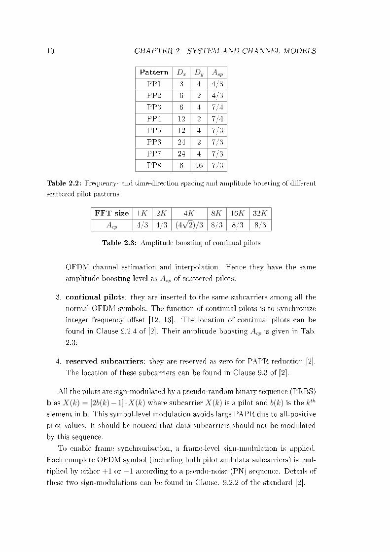
1. scattered pilots: they are inserted to normal symbols for OFDM channel
estimation with a given density in both frequency-direction (Dx) and time-
direction (Dy). The combinations of Dx and Dy and the pilot boosting
amplitude Asp are given in Tab. 2.2. The pilot pattern drawn in Fig. 2.3
is PP1 where Dx = 3 and Dy = 4;
2. edge pilots: they are the �rst and the last active subcarriers of each normal
OFDM symbol. The function of edge pilots is to assist scattered pilots for
10 CHAPTER 2. SYSTEM AND CHANNEL MODELS
Pattern Dx Dy Asp
PP1 3 4 4/3
PP2 6 2 4/3
PP3 6 4 7/4
PP4 12 2 7/4
PP5 12 4 7/3
PP6 24 2 7/3
PP7 24 4 7/3
PP8 6 16 7/3
Table 2.2: Frequency- and time-direction spacing and amplitude boosting of di�erent
scattered pilot patterns
FFT size 1K 2K 4K 8K 16K 32K
Acp 4/3 4/3 (4√
2)/3 8/3 8/3 8/3
Table 2.3: Amplitude boosting of continual pilots
OFDM channel estimation and interpolation. Hence they have the same
amplitude boosting level as Asp of scattered pilots;
3. continual pilots: they are inserted to the same subcarriers among all the
normal OFDM symbols. The function of continual pilots is to synchronize
integer frequency o�set [12, 13]. The location of continual pilots can be
found in Clause 9.2.4 of [2]. Their amplitude boosting Acp is given in Tab.
2.3;
4. reserved subcarriers: they are reserved as zero for PAPR reduction [2].
The location of these subcarriers can be found in Clause 9.3 of [2].
All the pilots are sign-modulated by a pseudo-random binary sequence (PRBS)
b as X(k) = [2b(k)−1] ·X(k) where subcarrier X(k) is a pilot and b(k) is the kth
element in b. This symbol-level modulation avoids large PAPR due to all-positive
pilot values. It should be noticed that data subcarriers should not be modulated
by this sequence.
To enable frame synchronization, a frame-level sign-modulation is applied.
Each complete OFDM symbol (including both pilot and data subcarriers) is mul-
tiplied by either +1 or −1 according to a pseudo-noise (PN) sequence. Details of
these two sign-modulations can be found in Clause. 9.2.2 of the standard [2].

2.1. SYSTEM MODEL 11
Similar to bit-interleaving, a two-step permutation algorithm is applied to data
cells to make them experience uncorrelated channel distortion. The permutation
consists of cell interleaving and time interleaving. Multiple T2 frames might be
involved in this process, which increases the complexity of simulating the system.
Instead, the requirement of experiencing uncorrelated channels is guaranteed by
a random data cell permutation within one T2 frame in this thesis.
2.1.3 Orthogonal-frequency-division-multiplexing (OFDM)
OFDM is a multi-carrier modulation technique using a large number of orthogo-
nal subcarriers closely-spaced by f0 = 1/NT . T = 7/64µs [2] is the time domain
baseband sample spacing and is also called the elementary time. N is the sub-
carrier number of a frequency domain OFDM symbol and is also called the FFT
size. In the frequency domain, each subcarrier is modulated by either a complex
data cell or a pilot. We denote the frequency domain OFDM symbol as a vector
X with elements X(k) where logical index k = [0, · · · , N−1] and N is a power of
2. From the last subsection we know that only the �rst Nuse subcarriers are ac-
tive, i.e., X(k)|k∈[Nuse,··· ,N−1] are zero, as shown in Fig. 2.4(a). The time domain
OFDM symbol is denoted by vector x of length N with elements x(n).
Adapted from the passband formula given in [2], baseband OFDM modulation
in DVB-T2 can be formulated as:
x(n) =5√27
Nuse−1∑k=0
X(k) exp
{i2π
(k − kmid)nN
}(2.2)
where i =√−1, kmid = (Nuse − 1)/2. The factor before the summation roughly
normalizes the average power of x(n) to unity and its value, 5/√
27, is calculated
from active-to-overall subcarrier ratio (Nuse/N) and pilot boosting level. Eq.
(2.2) indicates that the subcarrier with logical index k = kmid corresponds to the
direct-current (DC) component of a baseband OFDM symbol. In other words,
X(kmid) modulates the central carrier frequency in passband. Hence, modulated
subcarriers are symmetric around X(kmid) in physical spectrum as shown in Fig.
2.4(b).
Such modulation can be e�ciently implemented through N -point IFFT. Sup-
pose the input of an N -point IFFT is a vector G with elements G(n), we have:
G(n) =
X(n+ kmid) 0 6 n 6 N − kmid − 1
X(n− (N − kmid)) N − kmid 6 n 6 N − 1(2.3)

12 CHAPTER 2. SYSTEM AND CHANNEL MODELS
0 Kmid N-1Nuse-1
... ... ...Logical
index
(a) Frequency domain T2 OFDM symbol
0
fc
Nuse-1
... ... ...
Kmid
...
fc +Kmid*f0fc -Kmid*f0
Physical
frequency
(b) Physical spectrum
IFFT Processor
... ... ...Kmid
Nuse-1 N-1 0 Kmid-1
Input
port 0 N-1
Output
port 0 N-1
Active
subcarrier
Inactive
subcarrier
(c) Implementation via IFFT
Figure 2.4: Physical Spectrum and implementation of OFDM in DVB-T2
which means [X(kmid), · · · , X(N − 1)] �ll the front of IFFT inputs and [X(0),
· · · , X(kmid − 1)] �ll the tail sequentially, as shown in Fig. 2.4(c).
In the receiver side, OFDM demodulation can be implemented through N -
point FFT. The �rst N − kmid and the remaining kmid FFT outputs must be
swapped to restore the subcarriers.
Besides OFDM demodulation, the receiver also needs to compensate for tim-
ing and carrier frequency o�set introduced by imperfect channel and receiver.
Channel estimation is also compulsory which estimates frequency domain chan-
nel gain H(k). After synchronization and channel estimation, the received data
cells Y (k) modulating the kth subcarrier and the channel gain H(k) of the kth
subcarrier are ready for frame-demapping and then BICM demodulation.
2.2 Channel Models
Channel is the propagation environment that the transmitted signal experiences
before it is captured by the receiver. In most cases, DVB-T2 signal propagates in
wireless environments where there is re�ection, scattering and attenuation. The
receiver might be moving, which incurs Doppler frequency shifts and time varying
fading.
For simulation purposes, several channel types are carefully designed in the

2.2. CHANNEL MODELS 13
tap 0 1 3 4 5 7
ρ 0.248 0.129 0.31 0.425 0.49 0.0365
θ -2.57 -2.12 0.35 0.42 2.72 -1.44
tap 8 12 17 24 29 49
ρ 0.12 0.2 0.419 0.317 0.2 0.185
θ 1.13 -0.81 -1.55 -2.22 2.84 2.86
Table 2.4: Modi�ed multipath Rayleigh fading channel parameters
implementation guidelines of DVB-T2 [11] to imitate the channels in reality, in-
cluding additive white Gaussian noise (AWGN) channel, multipath Ricean fading
channel, multipath Rayleigh fading channel, mobile channel and 0dB echo chan-
nel [11]. In this thesis, we consider the �rst 4 types of channels. We further de�ne
an uncorrelated single-path Rayleigh fading channel to simulate and evaluate the
BICM module.
2.2.1 Additive White Gaussian Noise (AWGN) Channel
Channel is assumed to be perfect with impulse response h = 1. Only white
Gaussian noise generated by the receiver front end is added to the signal as:
y(n) = x(n) + w(n) (2.4)
where w(n) is Gaussian noise having a zero mean and a variance of σ2 per di-
mension. If x(n) is real, noise w(n) will be real, too. In this case, the total noise
variance of w(n) is N0 = σ2. If x(n) is complex, w(n) will be complex noise with
total variance N0 = 2σ2.
2.2.2 Multipath Rayleigh Fading Channel
Multipath Rayleigh fading channel has a long delay spread and does not have
a dominant path. The Rayleigh fading channel de�ned in the implementation
guidelines of DVB-T2 [11] consists of 20 non-zero paths and a maximum delay
spread of 5.42µs (Tab. 39 of [11]). It describes the portable indoor or outdoor re-
ceiver with a �xed location. Hence no Doppler frequency shift is involved and the
channel is time-invariant. However, the paths are not spaced by the elementary
time T = 7/64µs in our baseband model. It thus suits only the simulation for
passband transmission but not our baseband model. Hence, we combine paths
which have similar delays and adjust them to be spaced by a multiple of T . The

14 CHAPTER 2. SYSTEM AND CHANNEL MODELS
result is a 10-path Rayleigh fading channel with a maximum delay spread of 50T
as given in Tab. 2.4, where ρ and θ denote the amplitude and phase of each path,
respectively. The in�uence of such replacement will be presented in Chap. 7. Its
power delay pro�le and frequency domain channel transfer function are drawn in
Fig. 2.5.
0 10 20 30 40 500
0.1
0.2
0.3
0.4
0.5
Path index
Am
plitu
de
(a) Power delay pro�le
0 0.2 0.4 0.6 0.8 10
0.5
1
1.5
2
2.5
Normalized frequency
Am
plitu
de
(b) Channel transfer function
Figure 2.5: Time and frequency domain pro�le of Rayleigh fading channel
2.2.3 Multipath Ricean Fading Channel
Ricean channel is a multipath channel where the �rst path is dominant (usually
a line-of-sight path). The power of all the paths in Rayleigh fading channel are
summed up and multiplied with a factor Kricean = 10 to form the power of the
dominant path. This path is treated as zero-delay and is inserted in front of
the Rayleigh fading channel to form the Ricean fading channel. Its power delay
pro�le and frequency domain channel transfer function are drawn in Fig. 2.6.
0 10 20 30 40 500
0.2
0.4
0.6
0.8
1
Path index
Am
plitu
de
(a) Power delay pro�le
0 0.2 0.4 0.6 0.8 10
0.5
1
1.5
Normalized frequency
Am
plitu
de
(b) Channel transfer function
Figure 2.6: Time and frequency domain pro�le of Ricean fading channel

2.2. CHANNEL MODELS 15
2.2.4 Typical-urban 6-Path (TU-6) Mobile Channel
The movement of the receiver with respect to the transmitter incurs some fre-
quency shifts to the received signal. This phenomenon is called Doppler e�ect and
the frequency shift value is denoted by fd. A typical urban channel pro�le named
TU-6 is de�ned in the implementation guidelines [11] to model such channel. It
consists of 6 taps having wide dispersion in delay and relatively strong power.
Each of them follows the classical Jakes' Doppler spectrum [24]. In our model,
they are adjusted to be spaced by a multiple of the elementary time T . The �rst
tap is assumed to be zero-delay and the channel length is Lc = 47. Six taps
with non-zero power are positioned at n = 0, 2, 5, 15, 21, 46, with powers equal
to −3, 0, −2, −6, −8, −10 dB, respectively. Its power delay pro�le and average
frequency domain channel transfer function are drawn in Fig. 2.7.
0 10 20 30 40 500
0.2
0.4
0.6
0.8
1
Path index
Am
plitu
de
(a) Power delay pro�le
0 0.2 0.4 0.6 0.8 10.4
0.6
0.8
1
1.2
1.4
1.6
1.8
Normalized frequency
Am
plitu
de
(b) Channel transfer function
Figure 2.7: Time and frequency domain pro�le of TU-6 mobile channel
2.2.5 Uncorrelated Single-path Rayleigh Fading Channel
Data cells generated from BICM module are assumed to experience uncorrelated
channels. This assumption is guaranteed by cell and time interleaving in the
frame mapper. However, when we simulate BICM module solely without frame
mapper and OFDM modulation, such assumption does not hold anymore.
In this situation, an uncorrelated single-path Rayleigh fading channel is gen-
erated as an alternative. Suppose the coded data cells form a vector x with length
Ld, we generate a channel coe�cient vector h with a length of Ld, too. Its ele-
ments h(n) are independent complex Gaussian variables having a zero mean and
a variance of 1/2 in both real and imaginary parts. Then an element-wise multi-
plication is applied to x and h, followed by adding AWGN noise. The elements

16 CHAPTER 2. SYSTEM AND CHANNEL MODELS
of received signal y thus can be expressed as:
y(n) = x(n) · h(n) + w(n), 0 6 n 6 Ld − 1 (2.5)
In the receiver side, y(n) and h(n) are sent to the demapper to calculate the
LLR values of the bits carried by data cell x(n).

Chapter 3
BICM Module
3.1 Bose-Chaudhuri-Hocquenghem (BCH) Codes
3.1.1 Introduction
BCH codes are a group of linear block codes with polynomial structure in the
Galois �eld [4]. BCH codes used in DVB-T2 are binary systematic BCH codes,
performing as the outer encoder followed by the inner LDPC encoder. A complete
BCH codeword block cbch consists of two parts: message sequence mbch and
parity-check sequence pbch which is attached at the end of the message sequence
as:
cbch = [mbch(Kbch− 1), . . . ,mbch(1),mbch(0), pbch(Nbch−Kbch− 1), pbch(1), pbch(0)]
where the length of mbch and cbch is denoted by Kbch and Nbch, respectively.
The error-correcting ability tbch is 10 bit errors in BCH codes with block length
Nbch = 43200 and Nbch = 54000, and tbch = 12 in the rest of BCH codes. Table 3.1
summarizes the relationship between information length Kbch, block length Nbch
and error-correcting ability tbch of all the normal and short BCH codes de�ned in
DVB-T2.
Although none of the BCH codes have a block length of 2n − 1 which is an
essential characteristic of a primitive BCH code [4], all the BCH codes in DVB-T2
are actually primitive ones with their higher order bits set as zero and hidden.
Indeed, their complete block structure is:
[0, 0, · · · , 0︸ ︷︷ ︸2n−Nbch−1
,mbch(Kbch−1), . . . ,mbch(1),mbch(0), pbch(Nbch−Kbch−1), pbch(1), pbch(0)]
17

18 CHAPTER 3. BICM MODULE
Kbch Nbch tbch
32208 32400 12
38688 38880 12
43040 43200 10
48408 48600 12
51648 51840 12
53840 54000 10
Kbch Nbch tbch
3072 3240 12
7032 7200 12
9552 9720 12
10632 10800 12
11712 11880 12
12432 12600 12
13152 13320 12
Table 3.1: Lengths and error correcting abilities of BCH codes (left: normal; right:
short)
where n = 16 for normal BCH codes and n = 14 for short BCH codes. It
will be shown in later sections that these zero bits concern neither the encoder
nor the decoder, thus can be ignored. The primitive polynomial is Pn(x) =
x16 +x5 +x3 +x2 + 1 for normal BCH codes, and is Ps(x) = x14 +x5 +x3 +x+ 1
for short BCH codes .
3.1.2 Encoding
The encoding process on a message sequence mbch described by the standard is:
1. compute the generator polynomial g(x), which is the product of the �rst
tbch polynomials in Tab. 6(a) or 6(b) of the standard, subjected to whether
the BCH code is normal or short ;
2. pre-multiply the polynomial expression of mbch:
mbch(x) = mbch(Kbch − 1)xKbch−1 + . . .+mbch(1)x+mbch(0)x0
by xNbch−Kbch , or equivalently, pad Nbch −Kbch zeros after mbch in Matlab.
3. divide mbch(x) by g(x), calculate the remainder
pbch(x) = pbch(Nbch −Kbch − 1)xNbch−Kbch−1 + . . . pbch(1)x+ pbch(0)x0
the coe�cient sequence pbch is the parity-check sequence;
4. form codeword cbch by combining mbch and pbch together.

3.1. BOSE-CHAUDHURI-HOCQUENGHEM (BCH) CODES 19
In Matlab simulation, the 3rd step is a long polynomial de-convolution and
thus requires a prohibitively long operation time. Hence, a faster encoding ap-
proach is critical.
Consider an identity matrix Mbch of size Kbch ×Kbch:
Mbch =
1 0 0 . . . 0
0 1 0 . . . 0
0 0 1 . . . 0...
. . . . . . 1 0
0 . . . . . . 0 1
Each row in Mbch can be treated as a BCH message sequence and is naturally
orthogonal with each other. All the possible 2Kbch message sequences can be
expressed as a linear combination of the rows in Mbch. We then recall a basic
property of binary linear block codes [4]:
Theorem 3.1. If c1 and c2 are the codewords of message sequences m1 and m2
respectively, then the codeword of m3 = m1 + m2 is c3 = c1 + c2, where all the
additions are in Mod-2.
Taking advantages of this property, we can directly verify that the parity-
check sequence p3 = p1 + p2. Therefore, we can pre-calculate the parity-check
sequence of each row in Mbch and form a parity-bit matrix Pbch with size Kbch ×(Nbch − Kbch). The calculation of pbch of any particular message sequence mbch
becomes:
pbch = mbch ·Pbch (3.1)
3.1.3 Decoding
BCH decoder is a hard decoder where the input is the received binary codeword
vbch and the decoding output is also binary. The decoding algorithm we apply
is Berlekamp's iterative decoding algorithm [4]. The main ingredients of this
algorithm are two sequences and a set of equations:
1. syndrome sequence S = [S1, S2, . . . , S2tbch ] of length 2tbch;
2. coe�cient sequence σ = [σl, . . . , σ1, σ0], which is the vector expression of
error-locating polynomial σ(x) = σlxl + . . .+ σ1x
1 + σ0;
3. 2tbch of consecutive Newton's identities [4] which reveal the relationship
between S and σ:

20 CHAPTER 3. BICM MODULE
S1 + σ1 = 0
S2 + σ1S1 + 2σ2 = 0
S3 + σ1S2 + σ2S1 + 3σ3 = 0...
S2tbch + σ1S2tbch−1 + . . .+ σ2tbch−1S1 + 2tbchσ2tbch = 0
We brie�y describe the decoding process below, detailed algorithm can be
found in [4, 25]:
1. compute 2tbch consecutive syndromes using received sequence vbch and the
primitive element α, (α = 65581 and 16427 in normal and short BCH codes,
respectively);
2. compute error locating polynomial σ(x) in an iterative way: in the µth
iteration (µ 6 2tbch), �nd out σµ(x) that satis�es the �rst µ Newton's
identities;
3. perform Chien's Search [4] which tells that: if αl is a root of error-locating
polynomial σ(x), then the (2n − l)th bit (n = 16 or 14) in the codeword is
an error bit.
If there is no error, σ(x) = 0. If there are more than tbch errors, the degree
of σ(x) exceeds tbch. None of the roots of σ(x) will have the form of αl, where
l is a non-negative integer ranging from 0 to 2n − 1. Therefore σ(x) is unable
to indicate the error locations. In this case, the decoder is only able to detect
the existence of errors but is unable to correct them, thus it outputs vbch without
correction. Our simulations in the next subsection will also con�rm this property.
In the implementation of BCH decoder, Chien's search is time consuming
because 2n (n = 16 or 14) consecutive powers of the primitive element α: α0,
α1, . . ., α2n−1need to be checked to see whether they are the roots of the error-
locating polynomial. We suggest two solutions to this problem based on the
characteristics of the BCH codes:
• As discussed in Section 3.1.1, the BCH codes in DVB-T2 are zero-padded
primitive BCH codes. The polynomial expression of a codeword sequence
has degrees of at most Nbch − 1 and at least 0. This indicates that, in
Chien's Search, only α2n−(Nbch−1) to α2n−0 need to be substituted to the
error locating polynomial σ(x) to see whether they are the roots. The
potential roots of σ(x) ranging from α2n−(Nbch) to α0 do not need to be
checked.

3.1. BOSE-CHAUDHURI-HOCQUENGHEM (BCH) CODES 21
• To test α2n−(Nbch−1) to α2n−0, it is not e�cient to substitute them into σ(x)
one by one. Instead, we can construct a root-check matrixRbch to determine
the roots. Rbch is a matrix with Nbch rows and tbch + 1 columns:
Rbch =
(α2n−(Nbch−1))tbch (α2n−(Nbch−1))tbch−1 . . . . . . (α2n−(Nbch−1))0
. . . . . . . . . . . . . . . . . .
. . . . . . . . . . . . . . . . . .
(α2n−2)tbch (α2n−2)tbch−1 . . . . . . (α2n−2)0
(α2n−1)tbch (α2n−1)tbch−1 . . . . . . (α2n−1)0
(α2n−0)tbch (α2n−0)tbch−1 . . . . . . (α2n−0)0
The entries within a row of Rbch share a common base number αk (0 6
k 6 2n − (Nbch − 1)) with powers from 0 to tbch. The base number αk is a
potential root of σ(x). Multiplying the row by σ is equal to substitute αk
into σ(x). Consequently, we can compute a binary error sequence ebch as:
ebch = σ ·RTbch (3.2)
If the ith entry in the resulting 1 × Nbch column vector ebch is 1, then the
base number in the ith row of Rbch is a root of σ(x).
An examination on ebch shows that ebch is exactly the error pattern, i.e.,
cbch = vbch + ebch. Hence we could directly correct the errors using ebch without
base number identi�cation. Three Rbch matrices are enough for all the 13 types of
BCH codes in DVB-T2, one for normal BCH codes with tbch = 12, one for normal
BCH codes with tbch = 10 and one for short BCH codes. For example, the
normal BCH codes with tbch = 12 share a common Rnorm,12 with size 54000× 12.
If there is a received Nbch = 32400 BCH codeword with the highest degree of σ(x)
being l(l 6 tbch), instead of directly performing Chien's Search, we only need to
extract the last 32400 rows and the rightmost l + 1 columns of Rnorm,12 to form
a particular Rbch. Then we multiply it with σ to obtain the error pattern ebch.
3.1.4 Performance Evaluation
The performance of BCH codes are evaluated in terms of three measures:
• Given ε bit errors per BCH block, the error-correcting performance of the
BCH codes, including packet error rate (PER) and bit error rate (BER);
• In binary symmetric channel (BSC) with transition possibility p, the PER
and BER of the BCH codes;

22 CHAPTER 3. BICM MODULE
10 11 12 13 14 15 16 17 18 19 20 21 22 23 24 25
0
0.2
0.4
0.6
0.8
1
Block error number ε
Pac
ket e
rror
rat
e
PER (Nbch
=3240)
(a) PER with given no. of block errors ε
10 11 12 13 14 15 16 17 18 19 20 21 22 23 24 250
2
4
6
8x 10⁻³
Block error number ε
Bit
erro
r ra
te
BER (Nbch
=3240)
(b) BER with given no. of block errors ε
Figure 3.1: PER and BER of 3240 BCH with given no. of block errors ε
• The di�erences in performance among BCH codes with di�erent code lengths;
Matlab simulations are done based on short BCH codes. The results and
conclusions are valid for normal BCH codes as well.
Performance with Given Number of Block Errors
The decoding process described in Section 3.1.3 states that BCH decoder is able
to correct ε 6 tbch bit errors, and is able to detect the existence of ε > tbch errors
without correction. The simulation in this part aims to verify this statement.
Since what concerns the receiver are the message bits, the BER and PER com-
puted here are based on the message part of the codeword, with Nbch = 3240,
Kbch = 3024 and tbch = 12.
When there are ε > tbch errors in the codeword, there is only one situation
in which the decoder outputs correct message sequence. That is: all the ε errors
take place in the parity-check part but not the message part. The corresponding
probability Pnm is:
Pnm =
(Nbch−Kbch
ε
)(Nbchε
) (3.3)
where(mn
)means choosing n elements from a set containing m elements. Given
ε = 13, Nbch = 3240, Kbch = 3072, then Pnm ≈ 1.25 · 10−7, which is negligible.
With increasing ε, the possibility will become even smaller. Thus it is expected
that PER= 0 when ε 6 12 and nearly 100% when ε > 13. Fig. 3.1(a) demon-
strates simulation result of PER, which matches the expectation.
Fig. 3.1(b) shows the corresponding BER in message part. Unlike PER, BER
increases proportionally to the rising numbers of errors per block after ε = 12.
3.1. BOSE-CHAUDHURI-HOCQUENGHEM (BCH) CODES 23
10−4
10−3
10−2
10−1
10−40
10−20
100
Transition pobability p
Pro
babi
lity
Pε≤12 (N
bch=3240)
(a) Theoretical expectation of Pε612 of 3240
BCH
10−4
10−3
10−2
10−110
−6
10−4
10−2
100
Transition probabilty p
Err
or p
roba
bilit
y
Pε>12 (N
bch=3240)
PERBER
(b) PER and BER of 3240 BCH in BSC
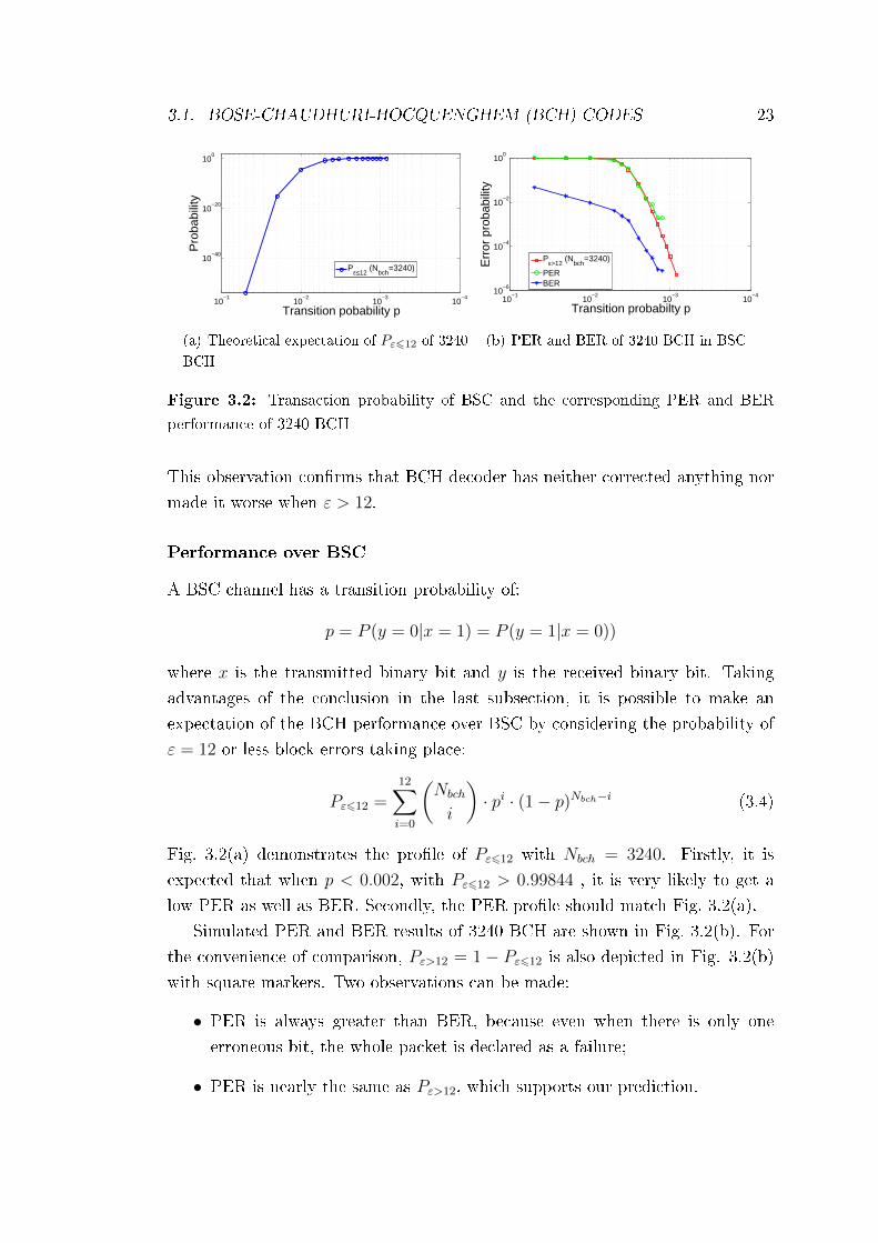
Figure 3.2: Transaction probability of BSC and the corresponding PER and BER
performance of 3240 BCH
This observation con�rms that BCH decoder has neither corrected anything nor
made it worse when ε > 12.
Performance over BSC
A BSC channel has a transition probability of:
p = P (y = 0|x = 1) = P (y = 1|x = 0))
where x is the transmitted binary bit and y is the received binary bit. Taking
advantages of the conclusion in the last subsection, it is possible to make an
expectation of the BCH performance over BSC by considering the probability of
ε = 12 or less block errors taking place:
Pε612 =12∑i=0
(Nbch
i
)· pi · (1− p)Nbch−i (3.4)
Fig. 3.2(a) demonstrates the pro�le of Pε612 with Nbch = 3240. Firstly, it is
expected that when p < 0.002, with Pε612 > 0.99844 , it is very likely to get a
low PER as well as BER. Secondly, the PER pro�le should match Fig. 3.2(a).
Simulated PER and BER results of 3240 BCH are shown in Fig. 3.2(b). For
the convenience of comparison, Pε>12 = 1− Pε612 is also depicted in Fig. 3.2(b)
with square markers. Two observations can be made:
• PER is always greater than BER, because even when there is only one
erroneous bit, the whole packet is declared as a failure;
• PER is nearly the same as Pε>12, which supports our prediction.

24 CHAPTER 3. BICM MODULE
10−4
10−3
10−210
−5
10−4
10−3
10−2
10−1
100
Transition probability p
Err
or p
roba
bilit
y
PER (Nbch
=7200)
Pε>12
(a) PER of 7200 BCH in BSC
10−4
10−3
10−210
−4
10−3
10−2
10−1
100
Transition probability p
Err
or P
roba
bilit
y
PER (Nbch
=9720)
Pε>12
(b) PER of 9720 BCH in BSC
10−4
10−3
10−2
10−3
10−2
10−1
100
Tansition probability p
Err
or p
roba
bilit
y
PER (Nbch
=10800)
Pε>12
(c) PER of 10800 BCH in BSC
10−4
10−3
10−2
10−3
10−2
10−1
100
Transition probability p
Err
or p
roba
bilit
y
PER (Nbch
=11880)
Pε>12
(d) PER of 11800 BCH in BSC
10−4
10−3
10−2
10−4
10−2
100
Transition probability p
Ero
or p
roba
bilty
PER (Nbch
=12600)
Pε>12
(e) PER of 12600 BCH in BSC
10−4
10−3
10−2
10−3
10−2
10−1
100
Transition probability p
Err
or p
roba
bilit
y
Pε>12
PER (Nbch
=13320)
(f) PER of 13320 BCH in BSC
Figure 3.3: PER performance of BCH codes with various lengths in BSC
Simulations on BCH codes with other block lengths show the same features
and will be plotted in the next subsection. In short, the error-correcting perfor-
mance of BCH codes follows the transition probability p, the smaller the p, the
better the performance.
Performance of BCH Codes in BSC with Di�erent Code Lengths
The relationship between PER and Pε>12 with block length of 7200, 9720, 10800,
11880, 12600 and 13320 are given in Fig. 3.3(a) to (f), respectively.
Our �rst observation is that PER curves match the probability Pε>12 in all
of the 6 �gures as expected. The second observation is that PER of 3240 BCH

3.1. BOSE-CHAUDHURI-HOCQUENGHEM (BCH) CODES 25
10−4
10−3
10−2
10−5
10−4
10−3
10−2
Transition probability p
Err
or p
roba
bilit
y
Blue curveswith roundmarks:
Red curvewithout mark:
Error probabilityof uncoded BSC
From left to right,the BER curves ofBCH codes withN
bch=3240
to13320
Figure 3.4: BER performance of BCH codes with various lengths in BSC
is much lower than that of 7200 BCH. With the increase of block length, PER
becomes slightly worse. This is because when the transition probability p is �xed,
longer codes, comparing with shorter ones, are more likely to incur ε > 12 errors,
which cannot be corrected.
This statement can be demonstrated more clearly with BER pro�les drawn
in Fig. 3.4. BCH with code length 3240 has a much lower BER than BCH with
code length 7200, because its code length is less than half of the second one.
The red line in Fig. 3.4 denotes the probability of un-coded bit error prob-
ability Pe in BSC, which is equal to the channel transition probability p. It is
noticeable that BER after decoding (blue ones) is nearly the same as Pe at the
beginning, but after some points, BCH decoder makes the BER to be lower than
Pe. The reason of performance improvement after certain points is quite simple:
channel transition probability p, joint with code length Nbch, exclusively decide
Pε>12. When Pε>12 falls down signi�cantly, it will be much more likely for the
BCH decoder to receive codeword with errors less than 13, thus the BER will be
reduced signi�cantly after decoding, too.

26 CHAPTER 3. BICM MODULE
3.1.5 Conclusion
The characteristics of BCH codes adopted in DVB-T2 were thoroughly studied
and optimized encoding and decoding processes were suggested. Simulations
showed that BCH codes are quasi-error free linear block codes with a designed
error-correcting ability tbch. BCH decoder ensures a full correction of any received
codeword with no more than tbch error bits. However, when the errors are more
than tbch, BCH decoder is only able to detect their existence but not able to
correct them.
3.2 Low-density Parity-check (LDPC) Codes
3.2.1 Introduction
LDPC codes, �rst introduced by Gallager in his Ph.D. thesis [5] in 1962, are
binary linear block codes. As its name suggests, it has a parity-check matrix
Hldpc whose row weight dr and column weight dc are much less than its row and
column numbers. Since dr and dc are not constant, the LDPC codes adopted in
DVB-T2 are irregular ones [4].
An LDPC codeword cldpc, with a length of Nldpc, consists of two parts:
• the left-most Kldpc bits are the message sequence:
mldpc = [mldpc(0),mldpc(1), . . . ,mldpc(Kldpc − 1)]
In DVB-T2, mldpc is exactly the encoded BCH codeword cbch
• the remaining Pldpc = Nldpc −Kldpc bits are the parity-check bits:
pldpc = [pldpc(0), pldpc(1), . . . , pldpc(Pldpc − 1)]
Coding parameters of all the 13 LDPC codes adopted in DVB-T2 are provided
in Tab. 3.2.
The parity-check matrix Hldpc, with a size of Pldpc×Nldpc, also consists of two
parts:
• the leftmost Pldpc × Kldpc sub-matrix is the transposed part, we denote it
by Ht;
• the rightmost Pldpc×Pldpc sub-matrix is the parity-check part, we denote itby Hp.
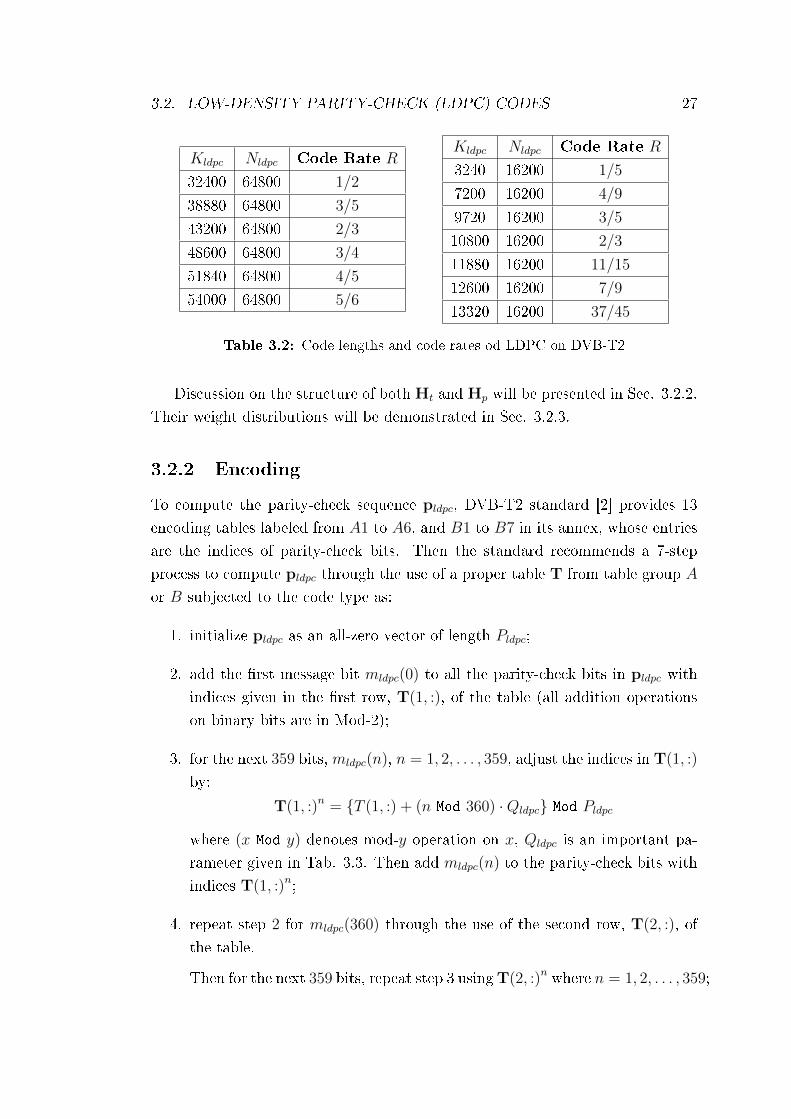
3.2. LOW-DENSITY PARITY-CHECK (LDPC) CODES 27
Kldpc Nldpc Code Rate R
32400 64800 1/2
38880 64800 3/5
43200 64800 2/3
48600 64800 3/4
51840 64800 4/5
54000 64800 5/6
Kldpc Nldpc Code Rate R
3240 16200 1/5
7200 16200 4/9
9720 16200 3/5
10800 16200 2/3
11880 16200 11/15
12600 16200 7/9
13320 16200 37/45
Table 3.2: Code lengths and code rates od LDPC on DVB-T2
Discussion on the structure of both Ht and Hp will be presented in Sec. 3.2.2.
Their weight distributions will be demonstrated in Sec. 3.2.3.
3.2.2 Encoding
To compute the parity-check sequence pldpc, DVB-T2 standard [2] provides 13
encoding tables labeled from A1 to A6, and B1 to B7 in its annex, whose entries
are the indices of parity-check bits. Then the standard recommends a 7-step
process to compute pldpc through the use of a proper table T from table group A
or B subjected to the code type as:
1. initialize pldpc as an all-zero vector of length Pldpc;
2. add the �rst message bit mldpc(0) to all the parity-check bits in pldpc with
indices given in the �rst row, T(1, :), of the table (all addition operations
on binary bits are in Mod-2);
3. for the next 359 bits, mldpc(n), n = 1, 2, . . . , 359, adjust the indices in T(1, :)
by:
T(1, :)n = {T (1, :) + (n Mod 360) ·Qldpc} Mod Pldpc
where (x Mod y) denotes mod-y operation on x, Qldpc is an important pa-
rameter given in Tab. 3.3. Then add mldpc(n) to the parity-check bits with
indices T(1, :)n;
4. repeat step 2 for mldpc(360) through the use of the second row, T(2, :), of
the table.
Then for the next 359 bits, repeat step 3 usingT(2, :)n where n = 1, 2, . . . , 359;

28 CHAPTER 3. BICM MODULE
Code Rate (normal LDPC) 1/2 3/5 2/3 3/4 4/5 5/6
Qldpc 90 72 60 45 36 30
Code Rate (short LDPC) 1/5 4/9 3/5 2/3 11/15 7/9 37/45
Qldpc 36 25 18 15 12 10 8
Table 3.3: Qldpc de�ned in DVB-T2 for LDPC codes with various code rates
5. in a similar manner, for every new 360 bits, use a new row of T, add
information bits to the corresponding parity-check bits;
6. after all message bits are used, the parity-check bits in pldpc are constructed.
Denote it as pold, then do:
pnew(i) =
pold(i), i = 0,
pnew(i− 1) + pold(i), i = 1, 2, . . . , Pldpc − 1
7. construct codeword cldpc by appending pnew after message sequence mldpc.
The encoding process is quite complex but can be simpli�ed. By examining
this process we found that the parity-check indices used for encoding each message
bit mldpc(n) indeed tells which parity-check bits is mldpc(n) involved in. Hence we
are able to shorten the encoding process by �nding out the parity-check matrix
Hldpc �rst. Recall a basic property of Hldpc [4]:
Theorem 3.2. A nonzero entry Hldpc(i, j) (0 6 i 6 Pldpc − 1 and 0 6 j 6
Kldpc − 1) in Hldpc means the jth message bit is involved in the ith parity-check
node.
Hence, by the use of a given table in the standard, we can determine the
parity-check matrix Hldpc of the corresponding LDPC code by:
1. construct two all-zero matrices: Ht (size Pldpc by Kldpc) and Hp (size Pldpc
by Pldpc);
2. �nd out the indices of parity-check bits concerning mldpc(n) in the same
way as suggested in the standard. Then set the corresponding entries in
the nth column of Ht as 1;
3. set Hp(0, 0) as 1. Also set Hp(i, i) and Hp(i, i− 1) (1 6 i 6 Pldpc − 1) as 1.
4. Hldpc = [Ht Hp]

3.2. LOW-DENSITY PARITY-CHECK (LDPC) CODES 29
Figure 3.5: Rough pro�le of parity-check matrix Hldpc of 32400 LDPC
Consequently, Ht and Hp are the transposed part and parity-check part of
Hldpc mentioned in Sec. 3.2.1. Following the above process, one can pre-calculate
all the parity-check matrices for all the 13 LDPC codes in DVB-T2, which are
needed for decoding process. All these low-density matrices can be saved and
used as sparse matrices in Matlab to save memory. A rough pro�le of Hldpc
for Kldpc = 32400 and Nldpc = 64800 LDPC code is shown in Fig. 3.5, where
nz = 226799 means there are 226799 ones in Hldpc while all the remaining entries
are zeros. The sparsity factor is thus 226799/(Pldpc ·Nldpc) ≈ 0.0108%.
After having found out Ht o�-line, the �rst 5 steps of the standard LDPC
encoding can be replaced by:
pldpc = mldpc ·Ht
followed by Step. 6 of �nding pnew and Step. 7 of constructing the codeword.
3.2.3 Decoding
Various methods are available for LDPC decoding, and they can be sorted into
two categories: hard-decision methods and soft-decision methods. As has been
pointed out in the literature [4, 19, 26], soft-decision decoding provides much
better error-correcting performance than hard-decision decoding at the expense of
30 CHAPTER 3. BICM MODULE
some computational complexity and iterative decoding delay. In this thesis, a soft-
decision decoding method called sum-product algorithm (SPA) [26] is employed.
SPA is a soft-in soft-out decoding algorithm. The input of SPA is a log-
likelihood rate (LLR) sequence L = [L(0), L(1), . . . , L(Nldpc − 1)] with elements:
L(j) = log
{Pr[cldpc(j) = 0]
Pr[cldpc(j) = 1]
}(3.5)
where Pr[cldpc(j) = 0] and Pr[cldpc(j) = 1] denote the probabilities that cldpc(j) is
0 and 1, respectively. log(·) is natural logarithm. The sign of the LLR represents
the decision on cldpc(j) (�+� for bit �0� and �-� for bit �1�), and its magnitude
represents the con�dence. The larger the magnitude, the more con�dent we are
on the decision of cldpc(j).
There are two important concepts involved in LDPC decoding: check-equation
(check-node) and bit-node [26]. A check-equation consists of some message and
parity-check bits whose Mod-2 summation, called a check-node Qi (0 6 i 6
Pldpc− 1), is always zero in any codeword. In an LDPC code, there are Pldpc such
equations, the elements in the ith check-equation have the same indices as in the
ith row of Hldpc. Similarly, there are Nldpc bit-nodes in an LDPC code. Each of
them is either a message or a parity-check bit.
The LLR provided by the demapper is called a priori information Lpr or
called intrinsic information. In SPA algorithm, it is passed among bit-nodes and
check-nodes to calculate the maximum a posteriori information Lpost [4, 26, 27],
which consists of intrinsic information of a bit coming from the demapper (thus
remains unchanged), and extrinsic information of the bit from the other bits in
the same check-equation. Then the a posteriori information is either fed-back to
check-nodes or is used as decoding output to make hard decision. The key step
in SPA algorithm is to calculate the extrinsic information, i.e., the information
about a bit cldpc(j) based on its relationship with a check-node Qi and the other
bits in this check-node. Such relationship is revealed by Gallager theorem [27]:
Theorem 3.3. Given a binary sequence x = [x1, x2, . . . , xn], if P (xk = 1) = pk,
then the probability that there is an even/odd number of �1�s in the sequence is:
Peven =1
2+
1
2
n∏k=1
(1− 2pk)
Podd = 1− Peven =1
2− 1
2
n∏k=1
(1− 2pk) (3.6)

3.2. LOW-DENSITY PARITY-CHECK (LDPC) CODES 31
To make a check-equation Qi tenable, there should be an even number of �1�s
in it. Hence the probability Pr(cldpc(j) = 1) (0 6 j 6 Nldpc−1 and cldpc(j) is one
of the bits in Qi) is equal to the probability that there are odd number of �1�s
in the remaining bits in Qi, and the probability Pr(cldpc(j) = 0) is equal to the
probability that there are even number of �1�s in the remaining bits in Qi. These
two probabilities can be easily calculated using the above equations and the LLR
information of the bits in Qi. Then we sum up the extrinsic information Lext(i, j)
of a bit cldpc(j) from each Qi to form the total extrinsic information Lext(:, j) of
this bit:
Lext(i, j) =
log{Pr[cldpc(j)=0|Qi]Pr[cldpc(j)=1|Qi]
}, cldpc(j) belongs to Qi
0 otherwise(3.7)
Lext(:, j) =
Pldpc−1∑i=0
Lext(i,j) (3.8)
The a posteriori information of a bit is the summation of its a priori infor-
mation and extrinsic information:
Lpost(j) = Lpr(j) + Lext(:, j) (3.9)
Consequently, Lpost(j) is sent to every related check-node Qi after subtracting
the extrinsic information from that check-node:
Lpost(i, j) = Lpost(j)− Lext(i, j)
To this end, LDPC decoding is complete. For iterative demapping and de-
coding which we will discuss in Sec. 3.3, Lext(:, j) is the extrinsic information of
a bit that LDPC decoder feeds-back to the demapper. From the next subsection,
we will turn to LDPC decoding performance evaluation.
3.2.4 Channel Capacity and Reliability
LDPC codes are near Shannon-limit codes. Before investigating LDPC decoding
performance, it is necessary to study the Shannon limit �rst. Shannon limit
bounds channel coding rate by channel capacity C which is the maximum rate
at which reliable communication, i.e., communication with arbitrary small error
probability, over the channel is possible [24].
Then, Shannon Noisy Channel Coding Theorem [4] tells that:

32 CHAPTER 3. BICM MODULE
R 1/4 1/2 3/5 2/3 3/4 4/5 5/6EbN0(dB) −0.793 0.188 0.682 1.084 1.628 2.045 2.402
Table 3.4: Shannon limit of DVB-T2 normal LDPC codes with BPSK modulation in
AWGN channel
Theorem 3.4. There exist channel codes and decoders that make it possible to
achieve reliable communication, with as small an error probability as desired, if
the transmission rate R < C, where C is the channel capacity. If R > C, it is
not possible to make the probability of error tend towards zeros with any code.
The basic channel mode considered here is a binary-input AWGN memoryless
channel with BPSK modulated input x ∈ {+√Es,−
√Es}, where without loss of
generality we can assume√Es = 1 and P (x =
√Es) = P (x = −
√Es) = 0.5, the
channel capacity in bits per channel use is:
C =1
2
∫ +∞
−∞p(y|
√Es) log2
p(y|√Es)
p(y)dy
+1
2
∫ +∞
−∞p(y| −
√Es) log2
p(y| −√Es)
p(y)dy (3.10)
It can be seen that C is a function of symbol-wise signal-to-noise ratio (SNR)
γs = Es/N0 where N0 is the total noise variance we have de�ned in Chap. 2.
When γs increases, C also increases monotonically.
In DVB-T2, code rate R is a given parameter with values such as 1/2, 3/5,
etc. given in Tab. 3.3. Hence, the task is to identify a channel capacity C > R
to ensure a reliable communication. This is equal to �nd out the minimum γs
which results in a C > R. Such γs is called the Shannon limit of channel coding.
There is another commonly used SNR in channel coding which is bit-wise:
γb =EbN0
=Es
MRN0
whereM is the number of bits per constellation point, e.g., M = 1 for BPSK and
M = 2 for QPSK. It is noticeable that Eq. (3.10) has no closed form; however it
can be evaluated numerically. The Shannon limit Eb/N0 subject to R in DVB-T2
are given in Tab. 3.4 [4].

3.2. LOW-DENSITY PARITY-CHECK (LDPC) CODES 33
3.2.5 Performance over Di�erent Channel Models and Mod-
ulation Methods
AWGN, BPSK
Simulations in this part aim to investigate the gap between the BER performance
of LDPC codes and Shannon limits introduced in the last subsection. Hence the
modulation method in use is BPSK, and the channel model is binary-input AWGN
memoryless channel. Then the elements of channel output vector y are expressed
as:
y(n) = x(n) + w(n), 0 6 n 6 Nldpc − 1 (3.11)
where x(n) = −(2 · cldpc(n) − 1) are the transmitted cells and w(n) is i.i.d real
white Gaussian noise with variance N0 = σ2. Then the probability that x(n) = 1
is transmitted provided that y(n) is received is:
P [x(n) = 1|y(n)]
=Pr[x(n) = 1, y(n)]
Pr[y(n)]
=Pr[y(n)|x(n) = 1] · Pr[x(n) = 1]
Pr[y(n)]
=Pr[y(n)|x(n) = 1] · Pr[x(n) = 1]
Pr[y(n)|x(n) = 1] · Pr[x(n) = 1] + Pr[y(n)|x(n) = −1] · Pr[x(n) = −1]
=
1√2πσ
exp (− |y(n)−1|22σ2 )
1√2πσ
exp (− |y(n)−1|22σ2 ) + 1√
2πσexp (− |y(n)+1|2
2σ2 )
=1
1 + exp(−2y(n)σ2 )
Similarly, one can �nd out that
Pr[x(n) = −1|y(n)] =1
1 + exp(2y(n)σ2 )
(3.12)
Hence, the initial LLR of each bit for decoding is:
L(n) = log
{P [cldpc(n) = 0|y(n)]
P [cldpc(n) = 1|y(n)]
}= log
{P [x(n) = 1|y(n)]
P [x(n) = −1|y(n)]
}= −2
y(n)
σ2

34 CHAPTER 3. BICM MODULE
0 2 4 6 8 10 1210
−6
10−5
10−4
10−3
10−2
10−1
Eb/N
0
BE
R
Shannon limit for rate 1/2 codeAWGN, BPSKAWGN, 16QAM2% fading, 16QAM
Figure 3.6: BER performance of R= 12 LDPC code with di�erent channel types and
modulation methods
The BER performance of rate 1/2 normal LDPC code with information length of
32400 is depicted in Fig. 3.6. Since BER converges at about 0.79dB, it is 0.6dB
away from Shannon limit.
AWGN, 16QAM
In practical use, higher order modulations such as QPSK and QAM are more
preferable than BPSK because of their spectrum e�ciency. In this subsection,
16QAM is employed while the channel model is still AWGN for the convenience
of comparison.
An LDPC codeword is modulated into a complex cell vector x according to
16QAM with Gray mapping. Each element x(n) bears 4 bits of information.
Then the cells are transmitted over complex AWGN channel and received as y
with elements y(n) as:
y(n) = xI(n) + i · xQ(n) + wI(n) + i · wQ(n), 0 6 n 6Nldpc
4− 1 (3.13)
where i =√−1, wI and wQ are the i.i.d. real and imaginary part of complex
Gaussian noise w(n) with variance per dimension of σ2 = N0/2. Since LDPC
decoder requires LLR of each bit, the mission of demapper is to calculate the LLR
of 4 bits based on 1 received cell. De�ne b(k) as the kth bit carried by received
3.2. LOW-DENSITY PARITY-CHECK (LDPC) CODES 35
cell y(n) (0 6 k 6 3 in 16QAM), χ as the full set of 16QAM constellation points,
and assume the a priori probability of Pr[b(k) = 0] = Pr[b(k) = 1] = 0.5, then:
Pr[b(k) = 0|y(n)] =Pr[y(n)|b(k) = 0]Pr[b(k) = 0]
Pr(y(n))
∝ Pr[y(n)|b(k) = 0]
=1
8Σ8s∈χ0
kPr[y(n)|s]
=1
8Σ8s∈χ0
k{Pr[yI(n)|sI ] · Pr[yQ(n)|sQ]}
=1
8Σ8s∈χ0
k
1√2πσ2
exp(−|yI(n)− sI |2
2σ2) · 1√
2πσ2exp(−|y
Q(n)− sQ|2
2σ2)
=1
8Σ8s∈χ0
k
1
πN0
exp(−|y(n)− s|2
N0
) (3.14)
where χ0k means a group of points in constellation χ whose kth bit is 0. Similarly,
we can obtain:
Pr[b(k) = 1|y(n)] ∝ 1
8Σ8s∈χ1
k
1
πN0
exp(−|y(n)− s|2
N0
) (3.15)
Consequently:
L(b(k)) = logPr[b(k) = 0|y(n)]
Pr[b(k) = 1|y(n)](3.16)
The BER performance of R = 1/2 normal LDPC code is plotted in Fig. 3.6.
BER converges at a γb of about 3.2dB, being 2.4dB worse than in the case of
BPSK.
Rayleigh Fading Channel, 16QAM
Rayleigh fading channel model is a typical model for wireless communication
where there are many objects in the environment that scatter the radio signal
before it is captured by the receiver. The transmitted signal x would experience
both magnitude and phase distortion as well as being corrupted by AWGN noise.
The elements in the received cell vector y can be modeled as:
y(n) = h(n)x(n) + w(n), 0 6 n 6Nldpc
4− 1 (3.17)
where h(n) is the fading coe�cient consisting of two i.i.d components, hI and hQ
with zero-mean and variance E[|hI |2] = E[|hQ|2] = 0.5, w(n) is complex additive
Gaussian noise with zero-mean and variance σ2 = N0/2 in both its real and
imaginary parts.

36 CHAPTER 3. BICM MODULE
Parameter Value Description
fs 106Hz channel sampling rate
fd 2 · 104Hz maximum Doppler frequency shift
npath 4 number of fading paths
Kldpc 32400 information sequence length of LDPC
Nldpc 64800 block length of LDPC
Modulation method 16QAM with Gray mapping
ldpc_k 50 maximum iterations of LDPC decoder
Table 3.5: Fading parameters of LDPC code in Rayleigh fading channel
In the receiver side, the process of demapper is almost the same as in AWGN
channel, except a slight modi�cation in the calculation of Pr[s|y(n)]. Instead of
the one in Eq. (3.14), we do:
Pr[s|y(n)] =1
πN0
exp(−|y(n)− h(n) · s|2
N0
) (3.18)
For simulations, the fading channel model is Jakes' model after the name
of William C. Jakes [24]. The fading rate is fd/fs = 2%, where fd is Doppler
frequency shift and fs is sampling rate. Other parameters are given in Tab. 3.5.
The BER performance of R = 1/2 LDPC code is given in Fig. 3.6. It is clear
that fading causes a 2.3dB SNR loss.
Check-sum Method
It has been observed in simulations that the number of errors in a block does
not always monotonically decrease when decoding iterations go on, but it re-rises
sometimes. In this case, the decoded codeword vldpc after the maximum number
of decoding iterations might have a large error number. To solve this problem,
we propose a method to trace the error number after each iteration in LDPC
decoding.
It is obvious that one cannot send the transmitted codeword cldpc to LDPC
decoder to get the actual error number in vldpc after each decoding iteration, but
instead, we can chase the number of parity-check equations not being satis�ed.
Given a parity-check matrix Hldpc, qldpc = vldpc ·HTldpc is a row vector of size
1×Pldpc. If the ith entry of qldpc is �1�, then the ith check-equation of Hldpc is not
satis�ed. Considering that multiplying the transmitted codeword cldpc by HTldpc

3.2. LOW-DENSITY PARITY-CHECK (LDPC) CODES 37
0 0.5 1 1.5 2 2.5 310
−6
10−5
10−4
10−3
10−2
Eb/N
0
BE
R
Shannon limit for rate 1/2 codeAWGN, BPSK, GA codewordAWGN, BPSK, check−sum method
Figure 3.7: BER performance of R= 12 LDPC code in BPSK using check-sum method
results in an all-zero vector, multiplying the received binary codeword vldpc with
Hldpc will result in a non-zero vector as:
qldpc = vldpc ·HTldpc = (cldpc + eldpc) ·HT
ldpc = eldpc ·HTldpc (3.19)
where vector eldpc is the error pattern in vldpc. The more the errors, the more the
�1� entries in the resulted vector. Indeed, in SPA iterative decoding algorithm,
we do calculate v ·HTldpc and terminate the algorithm when it is an all-zero vector.
In case the error number does not converge, this number is bounded to a
threshold away from zero which can be reached within a few iterations less then
the maximum iteration number. Hence, it is a waste of time if the decoding runs
further. We thus suggest that the number of �1� in qldpc after each iteration can
be recorded and one can terminate the decoding process once the number of �1� in
qldpc of current iteration is more that of the last iteration, or it is all-zero, before
the maximum iteration number is reached. This method is known as check-sum
method or syndrome-check method [4, 27].
Fig. 3.7 shows the BER performance of LDPC with BPSK modulation in
AWGN channel using this method compared with the one o�ering correct code-
word cldpc as genie to the decoder to aid the calculation of the number of remaining
errors after each iteration (GA codeword). There is no performance degradation
due to check-sum method.

38 CHAPTER 3. BICM MODULE
3.2.6 Conclusion
In this section, characteristics of LDPC codes adopted in DVB-T2 were studied.
Then optimizations on the encoding and decoding process were suggested. The-
oretical and empirical analysis stated that LDPC codes are near Shannon limit
linear block codes. Simulations on di�erent channel models indicated perfor-
mance degradation due to higher order modulations and fading channel. Lastly,
check-sum method was used to avoid nonconvergent LDPC decoding iterations.
3.3 BICM
3.3.1 Introduction
It was �rstly recognized by Zehavi [18] that the code diversity and reliability of
coded modulation over a Rayleigh fading channel could be improved by bit-wise
interleaving after channel encoding in the transmitter and by using soft demap-
ping in the receiver. This is the original concept of bit-interleaved coded modu-
lation. Then Caire et. al. developed a complete theory of BICM [19]. They pro-
vided a general information-theoretical framework for this concept and proposed
an iterative demapping and decoding (ID) scheme for it, as well as guidelines on
its design and evaluation. [19]. Bit-interleaved coded modulation/demodulation
considered in DVB-T2 involves the following steps:
• channel coding (LDPC code)
• bit-interleaving and de-interleaving
• multiplexing and de-multiplexing
• rotated and Q delayed constellation mapping
• iterative soft demapping and decoding
We have already discussed LDPC codes in the last section. Hence we will
start with bit-interleaving in the following subsection.
3.3.2 Bit Interleaver and De-multiplexer
Bit Interleaver
A bit interleaver permutates the location of the bits of an encoded codeword to
gain code diversity and reliability [18]. An ideal bit-interleaver makes all the bits
3.3. BICM 39
experience uncorrelated channels [18, 19].
Bit interleaving in DVB-T2 [2] is applied to 16, 64, and 256QAM only and it
consists of two steps:
1. parity interleaving : as its name suggests, parity interleaver spreads the
parity-check bits of an LDPC codeword while keeping the message bits
unchanged. Suppose the codeword is cldpc with block length Nldpc and
message length Kldpc, the resulted vector after interleaving is upi, then:upi(n) = cldpc(n), 0 6 n 6 Kldpc − 1
upi(Kldpc + 360t+ s) = cldpc(Kldpc +Qldpc · s+ t), 0 6 s 6 359, 0 6 t 6 Qldpc − 1
where Qldpc is de�ned in Tab. 3.3.
2. column twist : to achieve maximum diversity, bit interleaver operates a col-
umn twist on upi. upi is written column-wise into a matrix and then read out
row-wise. Column twist parameters are de�ned in Tab. 9 of the standard
[2].
After the two-step interleaving, the output is denoted by uct. This process can
be expressed in a function form as: uct = fbi(cldpc).
De-Multiplexing
Technically speaking, de-multiplexing is part of constellation mapping. However,
since it is also a bit-wise operation, we put it in this subsection. De-multiplexer
does not change the overall order of bits in uct, it only writes them into a ma-
trix with Nsubstream rows, and swaps the order of these rows to form the de-
multiplexing output matrix udm. Nsubstream is a multiple of constellation order
and is given in Tab. 3.6. The swap rule is given in Tab. 12 of the standard [2].
Analogue to bit interleaving, de-multiplexing process can also be expressed as a
function: udm = fdm(uct).
Matlab Simulation Method
Bit interleaver and de-multiplexer can be jointly expressed as a function: udm =
fdm[fbi(cldpc)]. In Matlab simulation, it is ine�cient to run this function every
time when a codeword needs to be interleaved and de-multiplexed. Moreover,
there are over 40 such functions for di�erent LDPC codes and constellations,
making the process very complex.

40 CHAPTER 3. BICM MODULE
Instead, noticing that the function udm = fdm[fbi(cldpc)] indeed is a one-to-one
projector on the bits from cldpc to udm , an alternative simulation method can
be suggested, which is simple yet e�cient. Take rate 1/2 normal LDPC with
16QAM mapping for instance:
1. Generate a index vector uidx = [1 : 64800];
2. perform uct = fbi(uidx) according to the standard;
3. perform udm = fdm(uct) according to the standard;
The elements in the resulting matrix udm records the projection rule of udm =
fdm[fbi(cldpc)]. We store this index matrix and name it Uint. Then in later
use, once a 1/2 normal LDPC codeword cldpc needs to be interleaved and de-
multiplexed into udm before 16QAM mapping, we only need to do (Matlab code):
udm = cldpc(Uint)
In the receiver side where multiplexing and bit de-interleaving are required, we
do (Matlab code):
cldpc(Uint) = udm
For other LDPC codes and modulation methods, we can �nd out their interleaving
index matrices in the same manner. After having done this o�-line, the bit
interleaving and multiplexing operations in both transmitter and receiver sides
will become very convenient. These matrices can be applied to the interleaving
and de-interleaving of LLR values passing between demapper and decoder in the
same way.
Modulation Nldpc Nsubstream
QPSK Any 2
16QAM Any 8
64QAM Any 16
256QAM64800 16
16200 8
Table 3.6: Number of substreams subjected to modulation methods and code lengths

3.3. BICM 41
Modulation QPSK 16QAM 64QAM 256QAM
Degree 29.0◦ 16.8◦ 8.6◦ arctan(1/16)
Table 3.7: Rotation degree for each modulation type
3.3.3 Rotated + Q-Delay Mapping
In classic QPSK and QAM modulations, I and Q components can be treated as
two independent pulse amplitude modulations [6, 7]. The mapping of I component
is exclusively decided by half of the bits in the binary index of the constellation
point; the Q component is exclusively decided by the remaining half of the bits.
This indicates that the estimation of I component in the receiver side gives no
information about Q component and vice-versa.
To make the most of I and Q components, e�orts are made to correlated these
two component [6, 7]. One approach is to change the constellation mapping from
Gray pattern to others. However, it has already been stated in [7] that Gray
mapping outperforms others when powerful FEC codes such as LDPC codes in
DVB-T2 are used. Hence, the solution to this task is to rotate the constellation.
The rotation degrees for di�erent constellations are given in Tab. 3.7. The
direction of the rotation is anti-clockwise, and rotation is not applicable for BPSK
modulation. An example of rotated 16QAM is plotted in Fig. 3.8.
To protect I and Q components from experiencing severe fading simultane-
ously, as well as to obtain diversity gain, a circular delay on the Q component is
introduced. Suppose the original modulated cell sequence of an LDPC codeword
is x with a length of Ncell, and xd is the cell sequence after Q-delay, we have:xd(n) = xI(n) + i · xQ(Ncell − 1), n = 0
xd(n) = xQ(n) + i · xQ(n− 1), 1 6 n 6 Ncell − 1
where i =√−1, Ncell = Nldpc/M is the number of modulated cells for each
LDPC codeword and M is the number of bits per cell. A delay interval of one
cell is de�ned in the standard [2] and is su�cient for I/Q independence over
uncorrelated Rayleigh fading channel. The reason of using uncorrelated fading
channel is explained below [7]:
In reality, Raleigh fading channel is correlated, but independent fading of
the I and Q components of the Q-delayed cells can still be guaranteed by cell,
time and frequency interleaving after Q-delay, all of which further diverse the

42 CHAPTER 3. BICM MODULE
−1.5 −1 −0.5 0 0.5 1 1.5−1.5
−1
−0.5
0
0.5
1
1.5
I axis
Q a
xis
Rotated 16QAM Constellation
00110001
00000010
10101000
10011011
11011111
11001110
0110
0111
0101
0100
Figure 3.8: Rotated 16QAM with Gray mapping
Q-delayed cells. Since the BICM system proposed in this section should be self-
contained, i.e., no cell, time and frequency interleaving should be used, we assume
uncorrelated fading channel to ensure I and Q components experience fading
independently. The simulation results using this approach reliably represent the
performance of the actual system, where fading channel is correlated but more
interleaving operations will be applied after Q-delay.
3.3.4 Iterative Demapping and Decoding
The concept of iterative decoding was �rst introduced for the decoding of code-
words generated from either a parallel or a serial concatenation of at least two
decoders which sandwich an interleaver [20]. This method could be well adapted
for BICM system if we treat the mapper as one of the decoders and LDPC de-
coder as the other one. The resulted system is known as BICM with iterative
decoding (BICM-ID) [19].

3.3. BICM 43
Information Passing between Demapper and Decoder
In the receiver side, there are two �decoders�, one is the demapper and the other
one is the LDPC decoder. The information passing through the demapper and
decoder is LLR based extrinsic information.
In LDPC decoder, the extrinsic LLR information of a bit is provided by the
LLR of all the other relevant bits in the same check-equation. Such extrinsic infor-
mation is then sent to demapper as the a priori LLR information. In demapper,
the extrinsic information of a bit is provided by all the other bits in the same cell.
We denote the input a priori information of demapper by Ldm,pr, the out-
put a posteriori information of demapper by Ldm,post, the extrinsic information
from demapper by Ldm,ext; the input a priori information of decoder by Ldc,pr,
the output a posteriori information of LDPC decoder by Ldc,post, the extrinsic
information from LDPC decoder by Ldc,ext, then:
Ldc,pr = Ldm,ext = Ldm,post − Ldm,prLdm,pr = Ldc,ext = Ldc,post − Ldc,pr (3.20)
To get iterations start, Ldm,pr is initialized as zero because there is no information
available from LDPC decoder in the �rst iteration.
Calculations of Ldm,post and Ldm,ext
The calculations of Ldc,ext and Ldc,post have already been presented in LDPC
section. We hereby derive the calculation of Ldm,post and Ldm,ext.
Suppose a 16QAM constellation set χ, including 16 points s with index b =
[b(1), b(2), b(3), b(4)], received cell y, and the a priori LLR of the 4 bits for the
demapper as L = [L(1), L(2), L(3), L(4)]. We demonstrate the calculation of
Ldm,post through an example, that is, the calculation of the a posteriori LLR of
b(1):
Ldm,post(b(1)) = logPr[b1 = 0|y]
Pr[b1 = 1|y]
= log
∑s∈χ0
1Pr(y|s)Pr(s)∑
s∈χ11Pr(y|s)Pr(s)
= log
∑s∈χ0
1[Pr(y|s)Pr(b)b←s]∑
s∈χ11[Pr(y|s)Pr(b)b←s]
(3.21)
= log
∑s∈χ0
1[Pr(y|s)
∏4k=1 Pr[b(k)]b←s]∑
s∈χ11[Pr(y|s)
∏4k=1 Pr[b(k)]b←s]
(3.22)

44 CHAPTER 3. BICM MODULE
where χ0k is a subset of constellation points in χ with the kth bit as 0, b ← s
means the binary index b of a constellation point s, Pr[b(k)]b←s equals either
Pr[b(k) = 1] or Pr[b(k) = 0] subjected to the kth element in a given b← s. Eq.
(3.21) to Eq. (3.22) holds because of the condition of independent bits mentioned
in Sec. 3.3.2.
However, extra computational load is required to �rst compute Pr[b(k) = ±1]
from L(k) for all k and all the received cells and then substitute them into Eq.
(3.22). Thus we suggest a much simpler way to compute Ldm,post which avoids
the calculation of Pr[b(k) = ±1].
Given a binary index b ← s, dividing Pr(b) by∏4
k=1 Pr(b(k) = 1) o�ers a
very useful equation:
Pr(b)∏4k=1 Pr[b(k) = 1]
= exp
[4∑
k=1
L(k) · b(k)
](3.23)
where x means the binary inverse of x. We demonstrate this through an example:
we divide the probability of b = [0, 1, 1, 0] by∏4
k=1 Pr[b(k) = 1]:∏4k=1 Pr[b(k)]b=[0110]∏4k=1 Pr[b(k) = 1]
=Pr[b(1) = 0]Pr[b(2) = 1]Pr[b(3) = 1]Pr[b(4) = 0]
Pr[b(1) = 1]Pr[b(2) = 1]Pr[b(3) = 1]Pr[b(4) = 1]
=Pr[b(1) = 0]
Pr[b(1) = 1]· Pr[b(4) = 0]
Pr[b(4) = 1]
= exp[L(1) + L(4)]
= exp[L(1) · b(1) + L(2) · b(2) + L(3) · b(3) + L(4) · b(4)]
= exp[4∑
k=1
L(k) · b(k)]
The expression exp[∑4
k=1 L(k) · b(k)] can be further shortened as exp[< L,b >]
where < ∗, ∗ > means inner product. Accordingly, by dividing both the numera-
tor and denominator of Eq. (3.22) by∏4
k=1 Pr[b(k) = 1] we can obtain:
Ldm,post(bk) = log
∑s∈χ0
k[Pr(y|s) exp(< L,b >)b←s]∑
s∈χ1k[Pr(y|s) exp(< L,b >)b←s]
(3.24)
The calculation of Pr[b(k) = ±1] is thus avoided. It should be pointed out that
although there are 16 s and 16 b involved in Eq. (3.22),∏4
k=1 Pr[b(k) = 1] is
constant since it is exclusively decided by L.
Consequently, Ldm,ext = Ldm,post − Ldm,pr is sent to LDPC decoder as the a
priori information.

3.3. BICM 45
Calculation of Pr(y|s)
The formula of calculating Pr(y|s) in classic constellation is:
Pr(y|s) =1
πσ2exp
{−|y − s|
2
2σ2
}(3.25)
where y is the received cell, s is a constellation point, σ2 = N0/2 is the variance
of both real and imaginary parts of AWGN noise. Due to rotation and Q-delay,
the calculation of Pr(y|s) in Eq. (3.22) and Eq. (3.24) is quite di�erent from the
one above and will be discussed in this subsection.
The received cell at time n can be modeled as:
y(n) = h(n) · xd(n) + w(n)
where xd(n) is the nth element of Q-delayed cell sequence xd. Fading coe�cient
h(n) comprises two i.i.d Gaussian distributed components hI(n) and hQ(n) with
zero mean and variance 0.5, which are assumed to be perfectly known by the re-
ceiver through channel estimation. Because uncorrelated Rayleigh fading channel
is assumed, there is no correlation between h(n) and h(n−τ) where τ is any time
delay. w(n) = wI(n) + i · wQ(n) is complex Gaussian noise with with zero mean
and variance σ2I = σ2
Q = σ2 = N0/2. Then we decompose the received cell into
its I/Q components as:
y(n) = h(n) · xd(n) + w(n)
= [hI(n)xId(n)− hQ(n)xQd (n) + wI(n)] + i · [hI(n)xQd (n) + hQ(n)xId(n) + wQ(n)]
= yI(n) + i · yQ(n) (3.26)
As can be seen in Eq. (3.26), the received yI(n) contains both xId(n) and xQd (n)
which are indeed xI(n) and xQ(n − 1) coming from two original cells. This is
also true for yQ(n). Hence, we cannot substitute such yI(n) and yQ(n) to the
classic formula Eq. (3.25) for demapping. Instead, since channel gain h(n) can
be expressed as h(n) = ρ(n)eiθ(n) where ρ and θ are its amplitude and phase
respectively, we introduce a new received cell yθ(n) as:
yθ(n) = y(n) · e−iθ(n) = ρ(n)(xId(n) + i · xQd (n)) + w(n)
= [ρ(n)xId(n) + wI(n)] + i · [ρ(n)xQd (n) + wQ(n)]
= yIθ(n) + i · yQθ (n) (3.27)
Here yIθ(n) contains xId(n) = xI(n) but not xQd (n) = xQ(n − 1), yQθ (n) contains
xQd (n) = xQ(n − 1) but not xId(n) = xI(n). Noise variance is not a�ected by

46 CHAPTER 3. BICM MODULE
phase rotation e−iθ(n) and thus is still σ2 in both I/Q components. Hence, the
probability that s ∈ χ before Q-delay is transmitted and is received as yIθ(n) and
yQθ (n+ 1) can be easily found as:
Pr[yIθ(n), yQθ (n+ 1)|s]
=1
πσ2exp
{−|y
Iθ(n)− ρ(n)sI |2 + |yQθ (n+ 1)− ρ(n+ 1)sQ|2
2σ2
}(3.28)
3.3.5 Simulation Results
Rate 4/5 LDPC code with block length Nldpc = 64800 and information length
Kldpc = 51840 is simulated with 16QAM mapping in uncorrelated Rayleigh fading
channel. The aim of the simulation is to compare the BER performance among
the following four BICM schemes:
1. classic 16QAM without iterative demapping and decoding (ID)
2. classic 16QAM with ID
3. rotated + Q-delayed 16QAM without ID
4. rotated + Q-delayed 16QAM with ID
BER performance after demapping is presented �rst, following by BER after
decoding.
BER after Demapping
Simulation in this section investigates the robustness of the two mapping methods
to fading channels. Hence, decoding is not taken into account and the BER is
evaluated after the soft demapper output over all the Nldpc bits. To investigate
the maximum BER gain brought by iterative demapping and decoding, perfect a
priori LLR information L of the transmitted bits is sent to the demapper (genie-
aided (GA) -LLR). Moreover, the magnitudes of L increase with SNR to match
the reality.
Fig. 3.9 shows the BER performance. Three observations can be made:
1. compared with classic 16QAM without GA-LLR, there is no SNR gain due
to GA-LLR. Thus we can safely infer that iterative demapping and decoding
will not improve the BER performance of classis 16QAM;

3.3. BICM 47
2. the BER of rotated and Q-delayed 16QAM without GA-LLR crosses the
classic ones at about 3.5dB, then it outperforms in high SNR region. The
SNR gain at BER of 10−4 is about 5dB. This is due to the code diversity
brought by Q-delay;
3. the BER of rotated and Q-delayed 16QAM with GA-LLR always outper-
forms the one without GA-LLR and the gap becomes larger in higher SNR
due to larger GA-LLR values. In reality, with increasing SNR, the LDPC
decoder provides Ldc,ext which approaches the GA-LLR with less errors and
larger magnitudes after each iteration. Hence, a BER performance improve-
ment on rotated and Q-delayed modulation due to ID can be predicted.
0 5 10 15 20 25 3010
−5
10−4
10−3
10−2
10−1
100
Eb/N
0
BE
R
Classic 16QAMGenie−aided Classic 16QAMRotated and Q−delayed 16QAMGenie−aided Rotated and Q−delayed 16QAM
Figure 3.9: BER after demapper of di�erent mapping schemes
BER after Decoding
For fair comparison, LDPC decoding iterations is 50 for both classic and rotated
and Q-delayed 16QAM without ID. For the ones with ID, Ldc,ext is fed back to
demapper after every 50 LDPC decoding iterations, and the number of demapping
iterations is 6. For each SNR point, simulations run until 50 erroneous LDPC
blocks take place or the maximum simulation size (500,000 LDPC blocks) is
reached.

48 CHAPTER 3. BICM MODULE
Fig. 3.10 supports the expected SNR gain on rotated and Q-delayed 16QAM
due to ID. We notice that [7] proposed an iterative demapping and decoding
approach which feeds-back Ldc,ext after every LDPC iteration, but this approach
failed to work in our simulation. We have observed that the BER after one
decoding iteration is almost as bad as before decoding, thus feeding this a poste-
riori information back can hardly bene�t the demapping process.
3.4 Implementation of BICM for P2 OFDM Sym-
bols
There are three major di�erences between the BICM module of L1 signaling
carried by P2 OFDM symbols and the normal BICM module:
1. Punctured short BCH codes are used. L1-signaling information bits are
split into several BCH message sequences with equal length Kbch,p2 which
is less than Kbch. Thus in each BCH codeword, the rest Kbch − Kbch,p2
bits are punctured following an algorithm described in Clause. 7.3.2 of the
standard and are not transmitted. Parity-check bits are not punctured. In
the receiver side, these punctured bits are recovered as zeros before BCH
8 8.25 8.5 8.75 9 9.25 9.5 9.75 1010
−7
10−6
10−5
10−4
10−3
10−2
10−1
Eb/N
0 (dB)
BE
R
Classical BICMRotated and Q−delayed without IDRotated and Q−delayed with ID
Figure 3.10: BER after decoding of di�erent mapping schemes

3.4. IMPLEMENTATION OF BICM FOR P2 OFDM SYMBOLS 49
decoding;
2. Punctured short (Nldpc = 16200) LDPC codes are used. BCH codeword
without puncturing is �rst LDPC encoded, then the BCH message bits are
punctured. Depending on the location of punctured BCH message bits,
some LDPC parity-check bits are punctured and are not transmitted. The
punctured LDPC parity-check bits are not always zero because there is
no check-equation which exclusively contains the punctured BCH message
bits. Indeed, punctured LDPC parity-check bits are �noise-like� where the
number of �0�s and �1�s are quite similar.
In the received side, only the locations but not the values of these bits are
known. Hence, these punctured LDPC parity-check bits are recovered as
�erased� before LDPC decoding, i.e., their LLR value is 0.
3. Rotated constellations are not used. Only classic BPSK, QPSK, 16QAM
and 64QAM are used to modulate coded L1 signaling information. No
special modi�cation needs to be taken since the normal module also has
classic constellations and the demapping formula is given in Eq. (3.25).
Other processes, including bit-interleaving and cell interleaving, are also applied
to P2. No modi�cations need to be taken.

50 CHAPTER 3. BICM MODULE

Chapter 4
Normal OFDM Symbols
4.1 OFDM Overview
DVB-T2 OFDM modulation and its implementation have already been studied
in Chap. 2. Hence, in this chapter we will focus on the e�ect of imperfect channel
and receiver, as well as the solutions to them, known as channel estimation and
synchronization, respectively.
In this chapter, we apply a general baseband OFDM system instead of the
one in DVB-T2 with speci�c structure for three reasons:
1. it is more reliable and useful to �rst develop synchronization and channel
estimation methods for general OFDM systems and then �nd their appli-
cation in a speci�c OFDM system;
2. it is much more clear to demonstrate and deduce equations using a general
OFDM system without concerning the speci�c structure of OFDM system
in DVB-T2;
3. DVB-T2 OFDM system is essentially derived from a general model. Tech-
niques applied to a general OFDM system can be easily applied to DVB-T2
OFDM system. The impact of the structure of DVB-T2 OFDM system
on these techniques, if any, and the corresponding modi�cations will be
emphasized.
In each general frequency domain OFDM symbol X, there are N subcarriers
independently modulated by either a pilot or data cell whose value is X(k), where
k ∈ [0, · · · , N − 1] is the subcarrier index. The corresponding discrete baseband
51

52 CHAPTER 4. NORMAL OFDM SYMBOLS
time domain symbol x is the inverse-fast-Fourier-transform (IFFT) of X given
as:
x(n) =1√N
N−1∑k=0
X(k) exp
(i2π
nk
N
), 0 6 n 6 N − 1 (4.1)
where i =√−1 is the imaginary unit and x(n) is zero-mean and its variance,
without loss of generality, is assumed to be 1. The time spacing between x(n)
and x(n+1) is the elementary period of the baseband model, denoted by T . Then
a replica of the last Ng symbols of x is padded ahead as a cyclic pre�x (CP). A
complete time domain OFDM symbol xcp = [xcp(−Ng), · · · , xcp(0), · · · , xcp(N −1)] thus has a length of Ns = Ng + N , where xcp(n) = x(n) for 0 6 n 6 N − 1
and xcp(n) = x(n+N) for −Ng 6 n 6 −1.
The length of CP is designed to be longer than the length Lc of time do-
main channel impulse response (CIR). In addition to eliminating inter-symbol-
interference (ISI), a CP with a su�cient length also maintains the circular con-
volutional relationship between x and CIR as:
y0 = x⊗ h + w (4.2)
where ⊗ denotes circular convolution and y0 is the received signal block with
length N after CP removal. The footnote 0 means timing o�set is zero. h is
discrete CIR with Lc taps spaced by T as we have de�ned in Chap. 2. Its total
power is σ2H =
∑Lc−1j=0 E[|h(j)|2]. Complex noise vector w contains identically dis-
tributed AWGN elements with variance N0 = 2σ2 where σ2 is the noise variance
per dimension. System SNR is thus de�ned as σ2H/N0 and we de�ne the normal-
ized noise variance as σ2n = N0/σ
2H . Denoting the N -point fast-Fourier-transform
(FFT) of y0, h and w by Y0, H and W, respectively, and by taking FFT on
both sides of (4.2), we obtain:
Y0(k) = X(k)H(k) +W (k), 0 6 k 6 N − 1 (4.3)
where W (k) is AWGN noise with normalized variance of σ2n.
4.2 Imperfect Receiver
An imperfect receiver introduces timing o�set and carrier frequency o�set (CFO),
as well as AWGN, to the received signal. We will analyze their e�ects �rst in the
following subsections before studying their solutions.

4.2. IMPERFECT RECEIVER 53
4.2.1 Timing O�set
For the convenience of demonstration, channel is assumed to be a scalar 1 and
there is no AWGN noise. The received signal y without CP removal is thus equal
to xcp. Assume the receiver makes a timing estimate of n. Then a length N
working sequence yn starting from y(n) is sent to FFT for OFDM demodulation.
If n = 0, we say there is not timing o�set.
If a timing o�set ∆n = −n ∈ [0, Ng] is present, the elements in yn become:
yn(n) = xcp(n−∆n) = x([n−∆n]N), 0 6 n 6 N − 1 (4.4)
where [·]N means Mod-N operation. If we use this working sequence for FFT
demodulation, timing o�set introduces only a phase rotation as:
Yn(k′) =1√N
N−1∑n=0
x([n−∆n]N) · e−i2πnk′N
=1
N
N−1∑n=0
[N−1∑k=0
X(k) · ei2πk(n−∆n)
N
]· e−i2π
nk′N
=1
N
N−1∑k=0
[X(k) · ei2π
−k∆nN
N−1∑n=0
ei2πn(k−k′)
N
]= ei2π
−k′∆nN X(k′) (4.5)
where Yn(k′) is the (k′)th FFT output. The second equation holds because
exp(i2π [x]NN
) = exp(i2π xN
). The last equation holds because circular summa-
tion∑N−1
n=0 ei2π
n(k−k′)N equals to N only when k− k′ is a multiple of N and is zero
for all other k. From the above equation, we can see clearly that Y (k′) does not
contain other modulated subcarriers. Hence, only a phase rotation is introduced
to every subcarrier by timing o�set but orthogonality among subcarriers is pre-
served. However, if condition ∆n = −n ∈ [0, Ng] is not satis�ed, time domain
samples from either the previous or the next OFDM symbol will be wrongly in-
cluded in the current OFDM symbol, incurring inter-symbol-interference (ISI)
and the destruction of subcarrier orthogonality. The situation in multipath chan-
nels is similar. However, the range of timing o�set which does not introduce ISI
is reduced to [0, Ng − Lc].
4.2.2 Carrier Frequency O�set
A CFO of ∆f away from central carrier frequency fc is introduced to the received
signal even in the absence of Doppler frequency shift when an imperfect receiver
54 CHAPTER 4. NORMAL OFDM SYMBOLS
oscillator down-converts passband signal into baseband. It causes a distortion of
ei2π∆ft to all the received signals. We can normalize it to the OFDM subcarrier
spacing 1/NT as:
ν =∆f
1/NT
= νi + νf (4.6)
Here νi is an integer and νf is a fractional number. They are called integer fre-
quency o�set and fractional frequency o�set, respectively. They will be synchro-
nized separately. The modeling of ν on discrete baseband time domain OFDM
samples can be expressed as:
y(n) = xcp(n)ei2πνnN , −Ng 6 n 6 N − 1 (4.7)
The E�ect of Integer Frequency O�set
To derive the e�ect of integer frequency o�set, we assume timing estimates n = 0
and the fractional frequency o�set νf is zero. Our working sequence yn thus has
elements:
y0(n) = x(n)ei2πνin
N , 0 6 n 6 N − 1 (4.8)
The (k′)th output Y0(k′) after FFT demodulation on y0 is:
Y0(k′) =1√N
N−1∑n=0
y0(n)e−i2πnk′N
=1
N
N−1∑n=0
[N−1∑k=0
X(k)ei2πnkN · ei2π
νin
N
]· e−i2π
nk′N
=1
N
N−1∑k=0
X(k)
[N−1∑n=0
ei2πn(k−(k′−νi))
N
]= X([k′ − νi]N) (4.9)
The last equation holds because circular summation∑N−1
n=0 ei2π
n(k−(k′−νi))N is always
zero unless k − (k′ − νi) is a multiple of N . The (k′)th FFT output is the (k′ −νi)
th transmitted subcarrier, indicating that an integer frequency o�set causes
subcarrier shift in the receiver. Such shift can be easily detected by using pilot
subcarriers.

4.3. SYNCHRONIZATION 55
The e�ect of Fractional Frequency O�set
To derive the e�ect of fractional frequency o�set, we assume integer frequency
o�set νi is zero and n = 0. Our working sequence yn thus has elements:
y0(n) = x(n)ei2πνfn
N , 0 6 n 6 N − 1 (4.10)
The (k′)th FFT output on working sequence y0 is:
Y0(k′) =1√N
N−1∑n=0
y0(n)e−i2πnk′N
=1
N
N−1∑n=0
[N−1∑k=0
X(k)ei2πnkN · ei2π
νfn
N
]· e−i2π
nk′N
=1
N
N−1∑k=0
X(k)
[N−1∑n=0
ei2πn(k−(k′−νf ))
N
]
=1
NX(k′)
N−1∑n=0
ei2πnνfN +
1
N
∑k 6=k′
N−1∑n=0
X(k)ei2πn(k−(k′−νf ))
N (4.11)
The main component of Y0(k′) is a distorted version of X(k′), i.e., the �rst term
in Eq. (4.11). Y0(k′) also contains other modulated subcarriers, i.e., the second
term in Eq. (4.11), indicating inter-carrier-interference (ICI). Such interference
will destroy the subcarrier orthogonality and thus should be suppressed as much
as possible before OFDM demodulation.
In summary, timing o�set introduces subcarrier rotation if it is within the
range of cyclic pre�x, otherwise it will introduce ISI. Integer frequency o�set
causes subcarrier shift in the frequency domain and can be conveniently estimated
by using pilots. Fractional frequency o�set incurs ICI which should be eliminated
as much as possible before OFDM demodulation. The synchronization of these
o�sets will be investigated in the next section.
4.3 Synchronization
In this section, we carefully review and compare timing and frequency synchro-
nization techniques proposed in the literature. The received signal y(n) is modeled
as:
y(n) = xcp(n)ei2πνnN + w(n), −Ng 6 n 6 N − 1 (4.12)
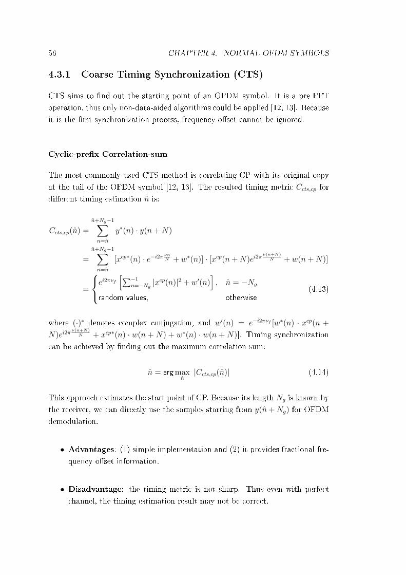
56 CHAPTER 4. NORMAL OFDM SYMBOLS
4.3.1 Coarse Timing Synchronization (CTS)
CTS aims to �nd out the starting point of an OFDM symbol. It is a pre-FFT
operation, thus only non-data-aided algorithms could be applied [12, 13]. Because
it is the �rst synchronization process, frequency o�set cannot be ignored.
Cyclic-pre�x Correlation-sum
The most commonly used CTS method is correlating CP with its original copy
at the tail of the OFDM symbol [12, 13]. The resulted timing metric Ccts,cp for
di�erent timing estimation n is:
Ccts,cp(n) =
n+Ng−1∑n=n
y∗(n) · y(n+N)
=
n+Ng−1∑n=n
[xcp∗(n) · e−i2πνnN + w∗(n)] · [xcp(n+N)ei2π
ν(n+N)N + w(n+N)]
=
ei2πνf[∑−1
n=−Ng |xcp(n)|2 + w′(n)
], n = −Ng
random values, otherwise(4.13)
where (·)∗ denotes complex conjugation, and w′(n) = e−i2πνf [w∗(n) · xcp(n +
N)ei2πν(n+N)
N + xcp∗(n) · w(n + N) + w∗(n) · w(n + N)]. Timing synchronization
can be achieved by �nding out the maximum correlation sum:
n = argmaxn|Ccts,cp(n)| (4.14)
This approach estimates the start point of CP. Because its length Ng is known by
the receiver, we can directly use the samples starting from y(n+Ng) for OFDM
demodulation.
• Advantages: (1) simple implementation and (2) it provides fractional fre-
quency o�set information.
• Disadvantage: the timing metric is not sharp. Thus even with perfect
channel, the timing estimation result may not be correct.

4.3. SYNCHRONIZATION 57
Frequency-domain Pilots Time-domain Correlation (FPTC)
Time domain OFDM symbol x can be treated as the superposition of the time
domain representation xd of data subcarriers and xp of pilot subcarriers [28] as:
xd(n) =1√N
∑k∈Pd
X(k) exp
(i2π
nk
N
)(4.15)
xp(n) =1√N
∑k∈Pp
X(k) exp
(i2π
nk
N
)(4.16)
where Pd and Pp are data and pilot subcarrier index sets, respectively. Because
xp is known by the receiver, we can achieve CTS by correlating the received signal
with xp [28, 29]. When timing estimate n = 0, the timing metric Ccts,fp can be
expressed as:
Ccts,fp(0) =N−1∑n=0
|xp(n)|2ei2πνnN + xd(n)x∗p(n)ei2π
νnN + w(n)x∗p(n)ei2π
νnN
=N−1∑n=0
|xp(n)|2ei2πνnN + w′(n) (4.17)
If CFO ν is zero, this timing metric is statistically equal to the autocorrelation
function of xp which is much sharper than the one in CP correlation-sum method.
Due to the existence of ν, the correlation cannot be summed up directly. Instead,
it is equally sliced into p portions, each portion has M samples where the phase
variation during M samples is assumed to be negligible [29]:
|P (k)| =
∣∣∣∣∣∣kM−1∑
n=(k−1)M
|xp(n)|2ei2πνnN + w′(n)
∣∣∣∣∣∣ , 0 6 k 6 p− 1
≈kM−1∑
n=(k−1)M
|xp(n)|2 (4.18)
where P (k) is the correlation sum of the kth portion. The absolute value of each
P (k) is then added together to indicate timing synchronization.
• Advantage: sharper timing metric than CP correlation-sum method;
• Disadvantages:
� performance degrades rapidly with increasing CFO;
� large implementation complexity and delay;

58 CHAPTER 4. NORMAL OFDM SYMBOLS
� when pilot patterns are not unique among adjacent OFDM symbols,
this method requires pilot pattern identi�cation before correlation.
The solution to this problem is correlatingDy consecutive OFDM sym-
bols which covers all the pilot patterns [29].
4.3.2 Fractional Frequency Synchronization (FFS)
CP Correlation-sum
As can be seen in Eq. (4.13), CTS metric of CP correlation-sum method provides
information about fractional frequency o�set νf [12, 13]. Hence, νf is estimated
through the CTS metric Ccts,cp as:
Ccts,cp(n) = ei2πνf
−1∑n=−Ng
|xcp(n)|2 + w′(n)
, n = −Ng
νf,est =1
2π∠Ccts,cp(n) (4.19)
where ∠(·) takes the angle of the term in the brackets. It is robust to AWGN but
its performance will degrade in multipath fading channels.
FPTC
In Eq. (4.18) of FPTC method, we can see that P (k+ 1) = P (k) · exp(i2πMνN
) in
the absence of noise. Thus by di�erentially correlating P (k), the CFO (including
integer and fractional parts) can be estimated as [29]:
Cffs,fp =
p−2∑k=0
P ∗(k) · P (k + 1)
νest =N
2πM∠Cffs,fp =
p
2π∠Cffs,fp (4.20)
Since ∠C ranges as [−π, π], the estimation range of CFO is [−p/2, p/2], which
is very limited.
However, we found that we cannot increase the number p of portions as much
as we want to increase the CFO estimation range. It is because a very small
M = N/p makes the portion sum in Eq. (4.18) noise-like.

4.3. SYNCHRONIZATION 59
4.3.3 Integer Frequency Synchronization (IFS)
Post-FFT Approach Using One Symbol
After CTS and FFS, fractional frequency o�set compensated working sequence
yn starting from y(n) is FFT demodulated. The output is denoted by vector Yn.
We de�neXcp as a lengthN vector where its entries in continual pilot locations
are continual pilots and are zeros otherwise. One-symbol IFS method [12, 13]
correlates shifted versions of Yn with Xcp. The shifted version which provides the
maximum correlation-sum indicates the subcarrier shift due to integer frequency
o�set:
Cifs,1(m) =N−1∑k=0
Yn([k +m]N) ·X∗cp(k), −N/2 6 m 6 N/2− 1
νi,est = argmaxm|C(m)| (4.21)
However, this method requires correct timing estimate because the phase rotation
due to timing o�set is di�erent among subcarriers, as shown in Eq. (4.5), which
will severely degrade the correlation-sum in Eq. (4.21).
Post-FFT Approach Using Two Symbols
We de�ne the continual pilot indices in frequency domain as Pcp. Two-symbol
IFS method [12, 13] correlates the frequency representations, Yn of the lth OFDM
symbol, and Yn+Ns of the (l+ 1)th OFDM symbol starting from n = (n+Ns), to
automatically cancel the in�uence of timing o�set 4n because both of the two
OFDM symbols su�er from the same timing o�set 4n. The resulted correlation
vector is denoted by Z with elements:
Z(k) = Y ∗n (k) · Yn+Ns(k)
=
±[A2cp +W ′(k)
], k ∈ Pcp + νi
random value, otherwise(4.22)
where Acp is continual pilots' amplitude,W′(k) = X∗l (k)Wl+1(k)+Xl+1(k)W ∗
l (k).
The sign ± takes place when frame-level sign-modulation is applied to the OFDM
symbols. For instance, if the lth and the (l+ 1)th OFDM symbols are modulated
by �-1� and �+1� respectively, then there will be a �−1� before the correlation.

60 CHAPTER 4. NORMAL OFDM SYMBOLS
Consequently the IFS can be obtained as [12, 13]:
Cifs,2(m) =∑k∈Pcp
Z([k +m]N), −N2
6 m 6N
2− 1
νi,est = argmaxm|Cifs,2(m)| (4.23)
If the channel is not AWGN, i.e., the frequency domain channel gain H(k) is
not 1, Eq. (4.22) can be rewritten as:
Z(k) =
±[H∗l (k)Hl+1(k) · A2
cp +W ′(k)]
k ∈ Pcp + νi
random value otherwise(4.24)
whereHl(k) andHl+1(k) are the kth subchannel gain of the lth and (l+1)th OFDM
symbols, W ′(k) = H∗l (k)X∗l (k)Wl+1(k)+Hl+1(k)Xl+1(k)W ∗l (k). In this case, this
method requires slow fading or static channels which satisfy Hl(k) ≈ Hl+1(k)
[12, 13].
4.3.4 Frame Synchronization
Available Metrics
The function of frame synchronization is to determine frame location and then
scattered pilot pattern which is critical for channel estimation. The key step
of frame synchronization is to �nd out the signs or sign changes of consecutive
OFDM symbols then compare them with the frame-level PN sequence [29]. Two
aforementioned synchronization metrics can be used for frame synchronization:
• the maximum shift-sum of the lth and the (l+1)th frequency OFDM symbols
in two-symbol IFS method, i.e., Cifs,2(νi,est). We denote it by Qfd(l);
• the sum of P (k) in FPTC method within the lth OFDM symbol. We denote
it by Qtd(l).
Di�erential Method
The goal of di�erential frame synchronization is detecting the phase inversion
between two adjacent OFDM symbols due to PN modulation.
Suppose p is the estimated PN sequence and its �rst element p(1) = 1.
For metric Qfd(l):
p(l + 1) =
p(l), |∠Qfd(l)| < π2
−p(l), |∠Qfd(l)| > π2
(4.25)

4.3. SYNCHRONIZATION 61
For metric Qtd(l):
p(l) =
p(l − 1), |∠[Qtd(l)]− ∠[Qtd(l − 1)]| < π2
−p(l − 1), |∠[Qtd(l)]− ∠[Qtd(l − 1)]| > π2
(4.26)
The position of maximum correlation-sum between p and the PN sequence
de�ned in the standard indicates the frame position. There will be no performance
degradation if we set p(1) = −1. It is because that setting p(1) = −1 will
introduce a sign inverse on the whole p. Consequently, only the sign but not the
magnitude of the correlation sums will be in�uenced and thus its performance is
exactly the same.
4.3.5 Fine Timing Synchronization (FTS)
FTS is needed in both AWGN and multipath channels. The aims of FTS are:
• eliminating ISI;
• �nding out the �rst channel tap, i.e., achieving perfect timing synchroniza-
tion.
The �rst task means we should at least guarantee that 0 6 4n 6 Ng − Lc asdiscussed in Sec. 4.2.1.
The realization of the second task enables us to use minimum mean squared
error (MMSE) channel estimation technique [30] which provides the best channel
estimation performance.
FTS is an analysis on time domain CIR or frequency domain channel transfer
function (CTF). A success in estimating the �rst channel tap in CIR directly
provides the perfect timing synchronization [28], as we will show in the channel
estimation section.
To Eliminate ISI
Most FTS strategies in the literature (see [12, 13, 28] and the references therein)
suggest recording the power sum of estimated CIR hn with length Le > Ng, or
estimated CTF Hn under di�erent timing estimation n.
FTS metric Cfts,td aims to �nd out the �rst actual channel tap in hn as:
Cfts,td(m) =m+Lc−1∑i=m
|hn0(i)|2, 0 6 m 6 Le − Lc + 1 (4.27)

62 CHAPTER 4. NORMAL OFDM SYMBOLS
−40 −20 0 20 400
0.2
0.4
0.6
0.8
1
Index m
Pow
er s
um
Figure 4.1: Fine timing metric pro�le of multipath Rayleigh fading channel without
noise
The index of the �rst channel tap is the m maximizing this metric and thus FTS
is achieved. Here hn is called the e�ective CIR, which we will discuss in detail in
the channel estimation section. Only one n is needed to perform FTS [12, 13].
Although it is claimed that this method reliably provides the location of the
�rst channel tap, it achieves this only when the channel length Lc is known. When
Lc is unknown, the Lc in Eq. (4.27) should be replaced by Ng. In this case, this
method only guarantees 0 6 4n 6 Ng − Lc that eliminates ISI. This is becausewhen channel length is Lc < Ng, Cfts,td(m) will have a plateau lasting Ng − Lcsamples in the absence of noise. Fig. 4.1 shows the perfect timing metric pro�le
of multipath Rayleigh fading channel without noise. When noise is present, this
plateau will �uctuate and thus there is hardly a way to decide the start/end of
this noisy plateau.
The FTS metric Cfts,fd(n) using frequency domain CTF is calculated as:
Cfts,fd(n) =∑k∈Psp
|Hn(k)|2 (4.28)
where Psp is scattered pilot index set. Then timing estimate is the n that max-
imizes this metric. While facing the same plateau problem as the time domain
one when Lc is unknown, this method asks for FFT demodulation and channel
estimation at every possible timing estimate n, which incurs considerable com-
putational load and processing delay.

4.4. CHANNEL ESTIMATION 63
To Find Out the First Tap
In the best case, the �rst channel tap is the strongest one, such as AWGN and
Rician channels. In this situation, most CIR estimation techniques can estimate
this tap reliably.
However, in multipath Rayleigh fading channels and mobile channels, the
�rst tap is not necessarily the strongest one and could be even as weak as a
noise tap sometimes. One approach to this problem is to design powerful CIR
estimation techniques which can accurately estimate CIR. The other way, which
is more feasible and motivating, is to design new channel estimation methods
less-sensitive to timing o�set, while being computationally e�cient, as we will
present in the next section.
4.4 Channel Estimation
4.4.1 OFDM Channel Estimation Overview
As we have just mentioned, OFDM systems are sensitive to synchronization errors
(especially timing errors) which severely degrade channel estimation performance.
One practical solution to this problem is to design channel estimation methods
which are robust to synchronization errors while keeping a low system complexity.
OFDM channel estimation involves estimating either channel impulse response
(CIR) in the time domain or its Fourier transform pair, channel transfer function
(CTF) in the frequency domain, where the ultimate goal is to use CTF for sub-
carrier demodulation. Direct CTF estimation techniques obtain an estimate of
data sub-channels by interpolating the least-squares (LS) estimate of pilot sub-
channels following some algorithms. Among the existing interpolation algorithms,
the minimum mean squared error (MMSE) [30] method o�ers the best bit-error-
rate (BER) performance. However, it requires perfect timing synchronization and
the knowledge of channel statistics (such as power delay pro�le). It is also known
to have a heavy computational load, as will be discussed later. These factors
restrict its application. A group of simple yet accurate interpolation algorithms
are linear (or higher order) frequency-direction-only (1D) interpolation [11] and
time-frequency-direction (2D) interpolation [11, 31]. While the performance of 1D
methods highly depends on pilot spacing, 2D methods provide higher accuracy at
the cost of longer processing delay and larger memory. In addition, time-direction
interpolation is adversely a�ected by large Doppler frequency shift.

64 CHAPTER 4. NORMAL OFDM SYMBOLS
For CIR estimation, one way is to perform inverse Fourier transform on the LS
estimate of pilot subchannels of multiple adjacent OFDM symbols [12, 32, 33].
While facing the same drawbacks encountered by time-direction interpolation,
this method usually produces a CIR which is not spaced by the system sampling
time, implying that certain channel taps would be lost. Another approach which
estimates CIR by correlating the received signal with the time domain representa-
tion of frequency domain pilots was introduced by Wang et. al. in [28]. Although
this method is robust to timing synchronization errors, the reserved subcarriers
in many commercial OFDM systems such as DVB-T2 [2] introduce unwanted
side-lobes around the estimated channel taps, requiring an extra de-convolution
algorithm for its suppression [28].
Recently, using the convolutional relationship between CIR and the trans-
mitted signal for channel estimation has attracted attention in the literature.
New CIR estimation algorithms have been proposed, which are robust to timing
synchronization errors and provide good channel estimation mean squared error
(MSE) performance. These methods include time domain least-squares (TDLS)
in [34] for normal OFDM symbols and in [16] for P1 preamble OFDM symbol
de�ned in DVB-T2 [2]. The main drawback of these matrix-based methods is the
computational and memory load because multiplications and inversions of matri-
ces with a size in the order of the OFDM symbol length are involved, which is also
true for matrix-based MMSE method. Furthermore, in TDLS, the random data
sequence in the transmitted time domain signal presents itself as an additional
noise term.
To overcome the aforementioned limitations, we propose a novel channel es-
timation method called domain-transform least-squares (DTLS). The main char-
acteristics of this method are as follows:
1. it uses only one OFDM symbol for channel estimation, thus it causes less
processing delay and is less sensitive to Doppler frequency shifts, especially
compared with the 2D interpolation technique;
2. it is robust to timing synchronization errors and does not require any knowl-
edge of channel statistics, which is superior to the MMSE method;
3. it works for any pilot pattern in frequency domain without extra computa-
tional cost;
4. it is a matrix-based method involving multiplications and inversions of ma-
trices with a size equal to the number of pilots. Therefore it saves huge

4.4. CHANNEL ESTIMATION 65
computational load compared with other matrix-based methods such as
MMSE and TDLS;
5. simulations on low- and high-Doppler mobile channels show that channel
estimation MSE and BER of DTLS method do not exhibit any error �oor
and are similar to TDLS method (which is a technique that shares properties
1, 2, and 3 with DTLS method).
4.4.2 Domain-transform Least-squares Estimation
E�ective Channel and Least-squares Channel Estimation
Before presenting our algorithm, we would like to discuss the concept of e�ective
channel [14] which is closely related to timing synchronization errors. This will
simplify the relationship between the transmitted and received signal where such
errors are present. It will also help us to understand the robustness of least-
squares estimation techniques to timing errors.
Recall the frequency domain relationship Eq. (4.3) among transmitted and
received signal and channel transfer function:
Y0(k) = X(k)H(k) +W (k), 0 6 k 6 N − 1
If X(k) is a pilot, H(k) = Y0(k)/X(k) will be the least-squares estimate of the
kth sub-channel. The pilot arrangement we considered is comb-type [35] where
pilots are uniformly inserted to subcarriers with a given density in both time-
and frequency- directions. There are in total Np pilots within one OFDM symbol
amplitude-boosted by a factor of β to gain higher SNR than data subcarriers
in the receiver. Np is also designed to be larger than both CP length Ng and
CIR length Lc to guarantee su�cient sampling on the frequency domain channel.
These properties are also owned by the scattered pilots in DVB-T2 OFDM system.
Imperfect timing synchronization provides an estimate n on the start point
of the received signal y where −(Ng − Lc) 6 n 6 0. The received signal block
yn = [y(n), · · · , y(n+N−1)] for OFDM demodulation is the circular convolution
of xcpn = [xcp(n), · · · , xcp(0), · · · , xcp(n + N − 1)] and the actual CIR h similar
to (4.2). Because xcp(n) = x(n + N) for −Ng 6 n 6 −1, we can rewrite the

66 CHAPTER 4. NORMAL OFDM SYMBOLS
convolution as:
yn = [x(n+N), · · · , x(N − 1)︸ ︷︷ ︸length |n|
, x(0), · · · x(n+N − 1)]⊗ h + w
= [x(0), ..., x(N − 1)]⊗ [0, · · · , 0︸ ︷︷ ︸|n| zeros
,h] + w
= x⊗ hn + w (4.29)
We de�ne this zero-padded hn as the e�ective channel impulse response under
the timing estimate n with e�ective length Le = Lc+ |n|. The maximum possible
value of Le is thus Ng. Correspondingly in frequency domain, suppose Yn is the
FFT output of yn and given a pilot subcarrier X(k), Hn(k) = Yn(k)/X(k) is
always the least-squares estimate of the kth subchannel of the e�ective channel
transfer function Hn. Hn(k) is unbiased with normalized noise variance σ2n/β
2
as long as the timing estimate satis�es −(Ng − Lc) 6 n 6 0. It is important
to have this condition guaranteed because any timing estimate out of this range
will introduce ISI. On the contrary, MMSE method [30] will fail when n 6= 0
because of the mismatch between the e�ective CIR and the channel power delay
pro�le, which is critical for computing the estimation matrix for obtaining data
subchannels.
Thus the robustness of least-squares channel estimation to timing synchro-
nization errors is established. We will capitalize on this property and introduce
our new channel estimation algorithm.
Proposed CIR and CTF Estimation Method
After performing FFT on yn to calculate Yn and then estimating pilot subchan-
nels using LS method as Hn(k) = Yn(k)/X(k), we obtain a length Np vector Hn,p
with entries Hn,p(m) being the LS estimate of the mth pilot subchannel. Our LS
estimate of the e�ective CIR is then given as:
hn = F−1 · Hn,p (4.30)
where (·)−1 denotes matrix inverse. Here F is an Np × Np Fourier transform
coe�cient matrix with F (m,n) = exp(−i2π np(m)
N
)and p(m) is the subcarrier
index of the mth pilot.
The length of the resulted CIR hn is Np while the maximum possible length
of hn is Ng. Thus we store the �rst Ng elements of hn as our estimated e�ective

4.4. CHANNEL ESTIMATION 67
CIR without further truncation since we do not know the exact channel length.
Subsequently, the whole e�ective CTF is estimated by applying N -point FFT on
the zero-padded estimated e�ective CIR.
In our method, F is a full rank square matrix and thus is invertible. For
comb-type pilot arrangement where all the pilots are uniformly distributed over
all the N subcarriers, the inverse F−1 is a well-conditioned matrix [36]. Thus
Eq. (4.30) is robust to the noise in the estimated Hn,p. However, in many
commercial OFDM systems, there are inactive (due to reserved subcarriers) and
irregular pilot locations. In DVB-T2, for example, about 15% of the subcarriers
are reserved as inactive ones. Meanwhile, the �rst and the last active subcarriers
in each OFDM symbol are set as edge pilots to assist the comb-type pilots for
channel estimation. These factors introduce linear similarity among some of the
rows in F. Hence, although F is still a full-rank square matrix, its inverse F−1
becomes ill-conditioned [36], i.e., the condition number [36] of F−1 is so large that
the noise in Hn,p will be severely ampli�ed and this results in an estimate of CIR
far away from its real value. We solve this problem by Tikhonov regularization
[37] as:
hn = (FHF + α · I)−1FH · Hn,p
= D · Hn,p (4.31)
where (·)H denotes Hermitian transpose and I is an Np ×Np identity matrix. α
is a regularization parameter the choice of which will be discussed in the next
subsection.
We name our method as domain-transform least-squares (DTLS), since it
employs the frequency-domain least-squares estimate of pilot subchannels to esti-
mate time domain channel impulse response, then transforms it back to frequency
domain. Although we design it for OFDM systems with comb-type pilot arrange-
ments, its implementation on other pilot patterns is straightforward. Speci�cally,
if the OFDM symbol is fully dedicated to pilot transmission, F becomes the full
Fourier transform matrix and thus its inverse F−1 equals its Hermitian transpose
FH . In this case, Eq. (4.30) is indeed the matrix expression of the IFFT from
CTF to CIR.
Some Strategies to Choose α
Minimizing the estimation error, e = ‖D·Hn,p−hn‖, where ‖·‖ denotes Euclideannorm, is highly dependant on choosing a proper regularization parameter α. To

68 CHAPTER 4. NORMAL OFDM SYMBOLS
10−0.5
10−0.4
10−0.3
10−0.2
10−0.1
100
100
102
104
er
e n
α=1.15
α=1.25e−10
α=2.25
Figure 4.2: An example of using L-curve method to choose α
investigate the e�ect of α, we decompose the estimation error into its two error
sources, which are known as regularization error er and additive noise error en:
e = ‖DHn,p − hn‖= ‖D(Hn,p + W)− F−1Hn,p‖6 ‖(D− F−1)Hn,p‖+ ‖D ·W‖= er + en (4.32)
It can be seen that, on one hand, er decreases with decreasing α because
D approaches F−1. On the other hand, en increases with decreasing α because
the condition number of D increases. One strategy to balance these two errors
is called L-curve method [37]. It plots E[er] and E[en] under di�erent α to
graphically search a trade-o� point which minimizes E[er] + E[en]. An example
of this method is depicted in Fig. 4.2. It is applied to a DVB-T2 OFDM system
with N = 1024 subcarriers where 73 of them are pilots with amplitude boosted
by β = 1.33, SNR is equal to 10 dB. The curve is L-shape, hence its name.
According to Fig. 4.2, an α around 2 is acceptable.
Using L-curve to �nd α for di�erent SNR values takes time. We thus follow
another strategy proposed in [36]. It derived a closed-form expression of α based
on the noise variance of the observation (Hn,p in our case). It o�ers a good

4.4. CHANNEL ESTIMATION 69
0 5 10 15 20 25 300
0.5
1
1.5
2
2.5
3
3.5
4
SNR (dB)
Reg
ular
izat
ion
para
met
er α
(a) α versus di�erent SNR
0 5 10 15 20 25 3010
−3
10−2
10−1
100
SNR (dB)
MS
E
(b) Upper-bound on MSE of h
Figure 4.3: Regularization parameter chosen and the upper-bound on MSE of h
trade-o� between er and en and sets an upper bound on the MSE of hn:
α =
(√Npσn
β
)2/3
var(hn) 6 N− 1
3p
(σnβ
) 43
(4.33)
An example of the regularization parameter chosen through this method and
the corresponding upper-bound on the MSE of hn are plotted in Fig. 4.3 for
various SNR values. It is applied to the same OFDM system used for L-curve
method. Speci�cally, for SNR equal to 10 dB, this method suggests an α = 1.6,
which is similar to the one obtained through L-curve method. Another important
observation is that α changes relatively slowly versus SNR, indicating that D can
be pre-calculated at some particular SNR values and used for similar SNRs. This
will further reduce processing delay and computational load.
4.4.3 Comparison with Other Techniques
In this subsection, we brie�y review some of the well-known channel estimation
techniques and compare them with DTLS regarding implementation issues. Per-
formance comparison including channel estimation MSE and BER will be pre-
sented in the next section. We have chosen representative techniques in their
category, as follows:
• time-frequency-direction linear interpolation (2D LI) [11], which is the most
commonly used method in the group of simple interpolation methods;

70 CHAPTER 4. NORMAL OFDM SYMBOLS
• minimum mean squared error (MMSE) estimation [30], which provides the
best MSE and BER performance, but relies on the knowledge of some chan-
nel statistics;
• time domain least-squares (TDLS) estimation [34], which is an e�ective
matrix-based time domain CIR estimation technique.
2D LI
In order to estimate data subchannels, 2D LI �rst performs time-direction (TD)
linear interpolation between the Dy spaced LS estimate of pilot subchannels fol-
lowed by performing frequency-direction (FD) interpolation. 2D LI needs to wait
for and store at least Dy OFDM symbols in order to perform time-direction in-
terpolation [11].
MMSE
In this subsection, we specify the CTF estimated through LS and MMSE meth-
ods by subscripts �ls� and �mmse�, respectively. We distinguish data and pilot
subcarriers by subscripts �d� and �p�, respectively. MMSE method employs Hp,ls
to estimate Hd,mmse as:
Hd,mmse = Rdp ·R−1/2pp︸ ︷︷ ︸
R
·R−1/2pp · Hp,ls
= M · Hp,ls (4.34)
where Rdp is the cross-correlation matrix of Hd and Hp, Rpp is the correlation
matrix betweenHp and its noise-a�ected version Hp,ls, both derived from channel
power delay pro�le and SNR information. Although the rank of under-braced
matrix R in Eq. (4.34) can be reduced by singular value decomposition to reduce
computational load, the reduction for pilot assisted OFDM systems is not e�ective
[30]. The size of the estimation matrix M is (N −Np)×Np.
TDLS
time domain OFDM signal x can be treated as the superposition of the time do-
main representation xp of the modulated pilot subcarriers and xd of the modulated
data subcarriers. Thus Eq. (4.29) can be written as yn = xp⊗hn +xd⊗hn +w.

4.4. CHANNEL ESTIMATION 71
Step MMSE 2D LI DTLS TDLS
1 yn=0FFT−→ Yn=0 yn
FFT−→ Yn ynFFT−→ Yn hn = T · yn
2 Hp,ls = Y/Xp Hn,p,ls = Yn/Xp Hn,p,ls = Yn/Xp hnFFT−→ Hn
3 Hd,mmse = M · Hp,ls TD interpolation hn = D · Hn,p,ls
4 FD interpolation hnFFT−→ Hn
Table 4.1: Key steps of considered channel estimation methods
Since xp is known to the receiver, an LS estimate of the e�ective CIR is:
hn = (PHP)−1PHyn
= T · yn (4.35)
Here P is an N×Np matrix with P (m,n) = xp([m−n]N) where [·]N means mod-
N operation. In [34], speci�c pilot arrangements and that all the N subcarriers
are active are assumed. However, these assumptions no longer hold in commer-
cial OFDM systems including DVB-T2, thus T is an ill-conditioned matrix and
regularization similar to DTLS is necessary.
Comparison
A list of the essential steps involved in each method is given in Tab. 4.1.
Compared with Dy OFDM symbols that 2D LI needs to perform, DTLS
method deals with only one OFDM symbol, reducing processing delay by at
least 50% since Dy > 2. Furthermore, high Doppler frequency shifts will degrade
the accuracy of time-direction interpolation, but will less a�ect one-symbol based
techniques such as DTLS.
A cross comparison among the three matrix-based methods, MMSE, TDLS
and DTLS, indicates that MMSE method requires the largest computational and
memory load, while DTLS method requires the least. First of all, in MMSE
method matrices Rdp and Rpp have to be calculated every time the channel
statistics change. Secondly, multiplications and inversions on matrices as large
as N × Np are involved. The size of the resulted estimation matrix T in TDLS
method is comparable with M in MMSE method. Both of them are much larger
than D in our proposed algorithm, whose size is only Np ×Np.
A �rst look at the key steps of each method may lead one to conclude that
TDLS method is the simplest because it does not require FFT on the received sig-
nal and LS estimate of pilot subchannels, which are commonly shared by MMSE,
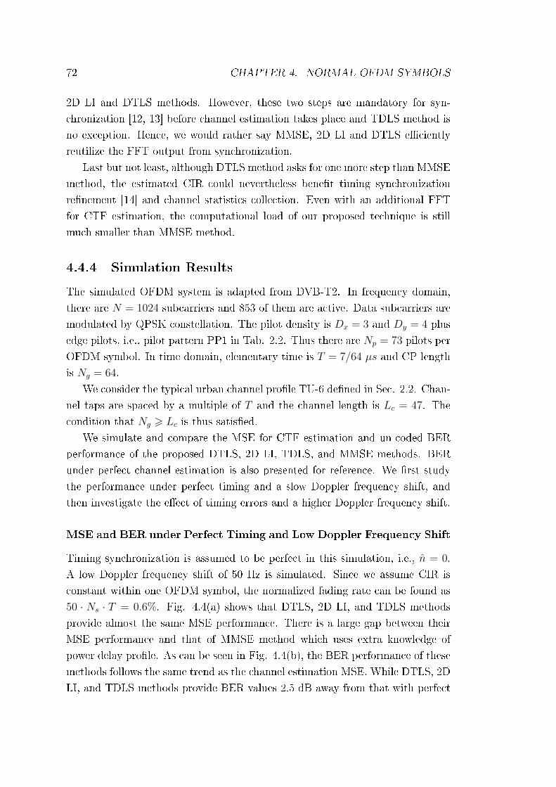
72 CHAPTER 4. NORMAL OFDM SYMBOLS
2D LI and DTLS methods. However, these two steps are mandatory for syn-
chronization [12, 13] before channel estimation takes place and TDLS method is
no exception. Hence, we would rather say MMSE, 2D LI and DTLS e�ciently
reutilize the FFT output from synchronization.
Last but not least, although DTLS method asks for one more step than MMSE
method, the estimated CIR could nevertheless bene�t timing synchronization
re�nement [14] and channel statistics collection. Even with an additional FFT
for CTF estimation, the computational load of our proposed technique is still
much smaller than MMSE method.
4.4.4 Simulation Results
The simulated OFDM system is adapted from DVB-T2. In frequency domain,
there are N = 1024 subcarriers and 853 of them are active. Data subcarriers are
modulated by QPSK constellation. The pilot density is Dx = 3 and Dy = 4 plus
edge pilots, i.e., pilot pattern PP1 in Tab. 2.2. Thus there are Np = 73 pilots per
OFDM symbol. In time domain, elementary time is T = 7/64 µs and CP length
is Ng = 64.
We consider the typical urban channel pro�le TU-6 de�ned in Sec. 2.2. Chan-
nel taps are spaced by a multiple of T and the channel length is Lc = 47. The
condition that Ng > Lc is thus satis�ed.
We simulate and compare the MSE for CTF estimation and un-coded BER
performance of the proposed DTLS, 2D LI, TDLS, and MMSE methods. BER
under perfect channel estimation is also presented for reference. We �rst study
the performance under perfect timing and a slow Doppler frequency shift, and
then investigate the e�ect of timing errors and a higher Doppler frequency shift.
MSE and BER under Perfect Timing and Low Doppler Frequency Shift
Timing synchronization is assumed to be perfect in this simulation, i.e., n = 0.
A low Doppler frequency shift of 50 Hz is simulated. Since we assume CIR is
constant within one OFDM symbol, the normalized fading rate can be found as
50 · Ns · T = 0.6%. Fig. 4.4(a) shows that DTLS, 2D LI, and TDLS methods
provide almost the same MSE performance. There is a large gap between their
MSE performance and that of MMSE method which uses extra knowledge of
power delay pro�le. As can be seen in Fig. 4.4(b), the BER performance of these
methods follows the same trend as the channel estimation MSE. While DTLS, 2D
LI, and TDLS methods provide BER values 2.5 dB away from that with perfect

4.4. CHANNEL ESTIMATION 73
0 5 10 15 20 25 3010
−5
10−4
10−3
10−2
10−1
100
SNR (dB)
Mea
n sq
uare
d er
ror
2D LITDLSDTLSMMSE
(a) MSE performance
0 5 10 15 20 25 3010
−4
10−3
10−2
10−1
100
SNR (dB)
Bit
erro
r ra
te
2D LITDLSDTLSMMSEPerfect CE
(b) BER performance
Figure 4.4: MSE and BER with perfect timing and 50Hz Doppler frequency shift

74 CHAPTER 4. NORMAL OFDM SYMBOLS
0 5 10 15 20 25 3010
−4
10−3
10−2
10−1
100
SNR (dB)
Mea
n sq
uare
d er
ror
2D LITDLSDTLSMMSE
(a) MSE performance
0 5 10 15 20 25 3010
−4
10−3
10−2
10−1
100
SNR(dB)
Bit
erro
r ra
te
2D LITDLSDTLSMMSEPerfect CE
(b) BER performance
Figure 4.5: MSE and BER with timing errors and 50Hz Doppler frequency shift
channel estimation, this di�erence becomes negligible for MMSE method. Hence,
MMSE method is the best choice provided that its computational requirements,
perfect timing and knowledge of channel statistics (as we will show below) are
satis�ed. Otherwise the proposed DTLS method is preferable compared to others.
The E�ect of Timing Synchronization Errors
In this simulation, imperfect timing estimate n within the ISI-free region is ran-
domly generated, i.e., −|Ng − Lc| 6 n < 0. To simulate 2D LI method, timing
estimate is aligned for all Dy OFDM symbols to ensure their e�ective CIR have
the same pro�le. The results are shown in Fig. 4.5. While DTLS, 2D LI, and
TDLS methods perform well despite the presence of timing synchronization er-

4.4. CHANNEL ESTIMATION 75
0 5 10 15 20 25 30
10−4
10−3
10−2
10−1
100
SNR (dB)
Mea
n sq
uare
d er
ror
2D LITDLSDTLSMMSE
(a) MSE performance
0 5 10 15 20 25 3010
−4
10−3
10−2
10−1
100
SNR (dB)
Bit
erro
r ra
te
2D LITDLSDTLSMMSEPerfect CE
(b) BER performance
Figure 4.6: MSE and BER with timing errors and 300Hz Doppler frequency shift
rors, MMSE method fails and results in a BER of about 50%. This veri�es the
sensitivity of MMSE estimation method to such errors.
Robustness to High Doppler Frequency Shift
Correct timing estimate and a high Doppler frequency of 300 Hz, i.e., a fading rate
of 3.6%, are assumed in this simulation. The MSE and BER results are drawn
in Fig. 4.6. While the one-symbol based estimation methods (TDLS, MMSE,
DTLS) provide similar performance as in the case of low Doppler frequency shift,
there are both MSE and BER �oors for 2D LI method in high SNR region. The
error �oor will be more severe for higher Doppler frequency shifts and larger Dy.
In summary, 2D LI and MMSE methods are not robust to high Doppler fre-

76 CHAPTER 4. NORMAL OFDM SYMBOLS
quency shift and timing synchronization errors, respectively. DTLS and TDLS
show comparable performance and both of them are robust to high Doppler fre-
quency shifts and timing errors. However, the implementation complexity of
DTLS is much lower than TDLS. In our simulations where Np/N ≈ 8.5%, the
size of the estimation matrix in DTLS is over 90% smaller than TDLS, leading
to huge savings on computational and memory load.
4.4.5 Conclusion
The proposed low complexity DTLS channel estimation technique for pilot-assisted
OFDM systems was thoroughly studied. The low complexity of DTLS method
is due to the small size of proposed matrix for obtaining CIR, compared to
other techniques that work with matrices whose size depends on the OFDM
symbol length. The performance of the proposed DTLS method was evaluated
and compared to other well-known channel estimation methods. Simulations on
DVB-T2 OFDM system over TU-6 mobile channels showed that DTLS method
provides similar channel estimation MSE and BER performance compared to
TDLS method, while enjoying much lower computational complexity and similar
robustness to timing synchronization errors, Doppler frequency shifts and pilot
arrangements. These features make DTLS an attractive choice in practice.
4.5 Implementation for P2 OFDM Symbols
The structure of P2 OFDM symbols is the same as normal ones except the ab-
sence of continual pilots. Thus the synchronization and channel estimation of P2
symbols are the same as the normal ones except that P2 symbols are not suitable
for frequency domain integer frequency synchronization. We can still use time
domain FPTC method although its performance is limited. Fortunately, there is
a P1 preamble OFDM symbol transmitted before P2 symbols and normal sym-
bols. It provides very good synchronization performance even in negative system
SNR. In the next chapter, we will propose a new P1 synchronization and decod-
ing method, whose key step can be e�ciently applied to P2 integer frequency
synchronization.

Chapter 5
P1 Symbol Synchronization and
Decoding
5.1 Introduction
In most OFDM systems, the time domain (TD) OFDM symbol is the superpo-
sition of modulated data and pilot symbols, as we have demonstrated in Sec.
4.3.1. Employing this property, the correlation between the received signal and
the TD symbol of frequency domain pilots was �rst used in [28] for channel im-
pulse response (CIR) estimation and then in [38] for timing synchronization. A
full synchronization scheme was later proposed in [29]. These methods are recom-
mended for the synchronization of normal OFDM symbols in the implementation
guidelines [11] of DVB-T2.
In the OFDM system of DVB-T2, the preamble P1 symbol carries the basic
system information such as transmission mode and FFT size and is transmit-
ted before each frame of P2 and normal OFDM symbols. To work under severe
transmission conditions, two replicas of the main part of TD P1 symbol are
frequency-shifted by fsh to form the head and tail of the TD P1 symbol [2]. [11]
demonstrates a baseline detection and synchronization scheme utilizing the cor-
relation between di�erent parts of the received signal, followed by a post-FFT
decoding process. Most P1 processing methods in the literature [15, 17, 39] em-
ploy the same correlation method. They mainly focus on timing synchronization
without being concerned about decoding.
However, since P1 symbol carries 7 bits of system information [2], there are
only 27 = 128 possible patterns for P1 active subcarriers in the frequency domain
(FD). Accordingly, there are only 128 possible TD P1 symbols which is known
77

78 CHAPTER 5. P1 SYMBOL SYNCHRONIZATION AND DECODING
by the receiver. Thus based on the correlation between the received signal and
the known TD P1 symbols, we propose a novel P1 synchronization and decoding
method. This method is insensitive to fsh o�set and continuous-wave (CW)
interference. Post-FFT decoding is also avoided and computer simulations show
that it achieves a decoding SNR gain of at least 6dB in AWGN channel and
at least 2dB in multipath Rayleigh fading channel compared with the decoding
performance given in the guidelines [11].
5.2 P1 Symbol Overview
5.2.1 Frequency Domain P1 Symbol
In the frequency domain, a P1 symbol encodes 7 bits. The �rst 3 bits, from
[000] to [111], form a sub-sequence called S1, indicating transmission mode. The
remaining 4 bits form S2, carrying information about FFT size. Hence there are
128 possible combinations of S1 and S2, corresponding to 128 di�erent binary
complementary sequences [2]mssseq with length 384, where 384 is also the number
of active subcarriers in FD P1 symbol. The autocorrelation of mssseq is a delta
function with a factor of 384, while the cross-correlation between di�erent mssseq
is always zero. mssseq is then di�erential BPSK modulated and scrambled to
form the active subcarriers of a 1K (K = 1024) OFDM symbol Xp. Xp is OFDM
modulated to form the main part p of a TD P1 symbol as:
p(n) =1√384
1023∑k=0
Xp(k) exp
(i2π
nk
1024
), 0 6 n 6 1023 (5.1)
where i =√−1. A detailed encoding process is demonstrated in the standard [2].
5.2.2 Time Domain P1 Symbol
In the time domain, a replica of the �rst 542 and the last 482 samples of p is
frequency shifted by fsh then padded before and after p, respectively, to form the
transmitted P1 symbol xp :
xp(n) =
p(n)ei2π
nfsh1024 n ∈ C2 = [0 ∼ 541]
p(n− 542) n ∈ C1 = [542 ∼ 1083]
p(n− 542) n ∈ B1 = [1084 ∼ 1565]
p(n− 1024)ei2πnfsh1024 n ∈ B2 = [1566 ∼ 2047]
(5.2)

5.2. P1 SYMBOL OVERVIEW 79
−2000 −1000 0 1000 20000
500
1000
1500
2000
Time index n
Mag
nitu
de
autocorrelation
(a) autocorrelation function
−2000 −1500 −1000 −500 0 500 1000 1500 20000
500
1000
1500
2000
Time index n
Mag
nitu
de
cross−correlation
(b) cross-correlation function
Figure 5.1: Time domain correlation property of P1 symbols
where fsh = 1/1024T , T is the elementary time domain sample spacing, and
[m ∼ n] means an index sequence from m to n.
Obviously there are 128 possible xp symbols, we label them as x0, x1, to x127,
corresponding to [S1 S2] = [0000000], [0000001], · · · , [1111111]. The correlation
properties of xp are shown in Fig. 5.1. The autocorrelation function has an
overwhelming correlation peak when n = 0 which is similar to a delta function.
On the other hand, the magnitude of cross-correlation function is much lower
than the autocorrelation function. These two properties enable time domain P1
decoding.
We further de�ne a �coarse� P1 symbol x128 which is the average of all the
128 possible P1 symbols and hence is known by the receiver:
x128 =1
128
127∑k=0
xk (5.3)
Due to the above correlation properties, x128 has a sharp correlation peak with
every P1 symbol when the timing is correct and has a small correlation when
the timing is incorrect, i.e., n = 0. This property is very important because it
provides a way to do TD synchronization without knowing which P1 symbol is
transmitted.
5.2.3 The Received Signal
The imperfect channel output yc can be modeled as:
yc = x ∗ h (5.4)
Here ∗ denotes linear convolution. The CIR h is a scalar equal to 1 in AWGN
channel. In multipath Rayleigh fading channel h is a vector of T -spaced channel
taps with complex Gaussian distributed channel gains.
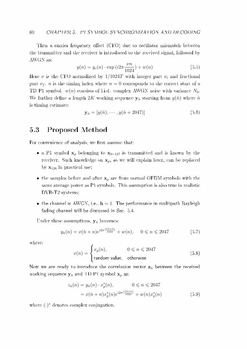
80 CHAPTER 5. P1 SYMBOL SYNCHRONIZATION AND DECODING
Then a carrier frequency o�set (CFO) due to oscillator mismatch between
the transmitter and the receiver is introduced to the received signal, followed by
AWGN as:
y(n) = yc(n) · exp (i2πνn
1024) + w(n) (5.5)
Here ν is the CFO normalized by 1/1024T with integer part νi and fractional
part νf . n is the timing index where n = 0 corresponds to the correct start of a
TD P1 symbol. w(n) consists of i.i.d. complex AWGN noise with variance N0.
We further de�ne a length 2K working sequence yn starting from y(n) where n
is timing estimate:
yn = [y(n), · · · , y(n+ 2047)] (5.6)
5.3 Proposed Method
For convenience of analysis, we �rst assume that:
• a P1 symbol xp belonging to x0∼127 is transmitted and is known by the
receiver. Such knowledge on xp, as we will explain later, can be replaced
by x128 in practical use;
• the samples before and after xp are from normal OFDM symbols with the
same average power as P1 symbols. This assumption is also true in realistic
DVB-T2 systems;
• the channel is AWGN, i.e., h = 1. The performance in multipath Rayleigh
fading channel will be discussed in Sec. 5.4.
Under these assumptions, yn becomes:
yn(n) = x(n+ n)ei2πν(n+n)
1024 + w(n), 0 6 n 6 2047 (5.7)
where:
x(n) =
xp(n), 0 6 n 6 2047
random value, otherwise(5.8)
Now we are ready to introduce the correlation vector zn between the received
working sequence yn and TD P1 symbol xp as:
zn(n) = yn(n) · x∗p(n), 0 6 n 6 2047
= x(n+ n)x∗p(n)ei2πν(n+n)
1024 + w(n)x∗p(n) (5.9)
where (·)∗ denotes complex conjugation.

5.3. PROPOSED METHOD 81
5.3.1 CTS and IFS
When the timing is correct, i.e., n = 0, the elements of zn=0 can be written as:
z0(n) = |xp(n)|2ei2πνn
1024 + w(n)x∗p(n), 0 6 n 6 2047 (5.10)
After multiplying with noise vector w, the distinctive frequency components in
x∗p, i.e., the active subcarriers, in the second term of the righthand side of Eq.
(5.10) are distributed across all frequencies in z0. Hence the only distinctive
frequency component in z0 is ν. On the other hand, when n 6= 0 or there is no P1
symbol, zn will not have a distinctive frequency component. Hence, the existence
of such frequency component in zn can be used as a metric for P1 detection and
coarse timing synchronization (CTS), while the distinctive frequency value can
be used for CFO synchronization.
To identify such frequency component in a working sequence, [40] proposed a
direct trial-and-error frequency search method on OFDM training symbols which
is time-consuming depending on the search resolution. However, we �nd that the
frequency search can be e�ciently implemented by a 2K FFT on zn. We denote
the magnitude of the 2K FFT output sequence as Zn with elements:
Zn(k) =
∣∣∣∣∣2047∑n=0
zn(n)e−i2πnk
2048
∣∣∣∣∣ , 0 6 k 6 2047 (5.11)
We �rst show how our frequency search method works if ν is a multiple of 0.5.
Suppose k0 = 2ν is an integer, when n = 0, the kth0 FFT output Z0(k0) becomes:
Z0(k0) =
∣∣∣∣∣2047∑n=0
[|xp(n)|2ei2π
νn1024 + w(n)x∗p(n)
]e−i2π
nk02048
∣∣∣∣∣=
∣∣∣∣∣[
2047∑n=0
|xp(n)|2ei2πνn
1024−i2π νn
1024 + w′(n)
]∣∣∣∣∣≈
2047∑i=0
|xp(n)|2 (5.12)
The last equation holds because w′(n) = w(n)x∗p(n)e−j2πnk02048 is still AWGN noise
and its sum over thousands of samples is statistically zero. In Eq. (5.12),
FFT process compensates for CFO in the output Z0(k0), and its magnitude,∑2047n=0 |xp(n)|2, is the maximum value we can get. Such compensation and maxi-
mization does not happen in other Z0(k) where k 6= k0, as shown in Fig. 5.2(a).
In addition, when there is no distinctive frequency component in z0 due to wrong

82 CHAPTER 5. P1 SYMBOL SYNCHRONIZATION AND DECODING
0 2 4 6 8 10 12 140
500
1000
1500
2000
FFT output index k
Mag
nitu
de
Frequency components
(a) correct timing estimate
0 500 1000 1500 20000
500
1000
1500
2000
FFT output index k
Mag
nitu
de
frequency components
(b) wrong timing estimate
Figure 5.2: FFT output under di�erent timings, ν = 3, SNR=-6dB
timing estimate or due to the absence of P1 symbol, such compensation and
maximization does not happen, neither, as shown in Fig. 5.2(b).
CFO is unlikely to be an integer in reality, so there will be residual frac-
tional CFO remaining in (5.12). Since 2K FFT is performed over a time period
of 2048T , our normalized frequency search resolution is 0.5, implying that the
residual νf is no more than ±0.25. In the worst case that νf is 0.25 before FFT,
there will be two distinctive FFT outputs, Z0(2ν±0.5), with the same magnitude
that is larger than∑2047
n=0 |xp(n)|2/2. They do not degrade the CTS performance
because both of them are su�ciently larger than the remaining FFT outputs
when n = 0 and all the FFT outputs when n 6= 0. For integer frequency syn-
chronization (IFS), both νi,est = ν ± 0.25 are acceptable and the residual νf is
∓0.25.
Next, maxk{Zn(k)} can be used to indicate the existence of a �distinctive�
frequency component. Our CTS metric C(n) and IFS metric I(n) for a given n
are:
C(n) = maxk{Zn(k)} (5.13)
I(n) = argmaxk{Zn(k)}, 0 6 k 6 2047 (5.14)
Then CTS and IFS are achieved as:
n = argmaxn{C(n)} (5.15)
νi,est =
I(n)/2, 0 6 I(n) 6 1023
[I(n)− 2048]/2, 1024 6 I(n) 6 2047(5.16)
which means the normalized estimation range of our IFS is ±512. For P1 detec-
tion, an experimentally found threshold on C(n) is reliably used and we will not
discuss it further.

5.3. PROPOSED METHOD 83
Since the receiver does not know which P1 symbol is transmitted, we replace
xp by x128 to perform the described correlation in practical use. Taking advantage
of the correlation properties of x128 mentioned in Section 5.2, C(n) will be a high
value i� there is a P1 symbol in the received signal and n = 0, but is small
otherwise.
Compared with the standard synchronization method [11], the main advan-
tages of the proposed CTS and IFS are:
• down-shifting C2 and B2 zones by fsh is avoided, thus the proposed method
is insensitive to fsh o�set;
• the proposed method is insensitive to continuous-wave (CW) interference
because the power of fcw will spread to all the frequencies in x∗p after corre-
lating, thus it hardly exceeds the power of ν in z0, while in the implemen-
tation guidelines [11] an interference deleting process is required.
• numerical results show that the proposed CTS can lock to the correct timing
in AWGN channel and the �rst main path in multipath Rayleigh fading
channel.
5.3.2 FFS
After performing CTS and IFS, we obtain integer CFO νi compensated y0 and
z0 with residual |νf | 6 0.25. Without noise:
z0(n) = |xp(n)|2 exp(i2πnνf1024
), 0 6 n 6 2047 (5.17)
Fractional frequency synchronization is performed through a two-branch method
similar to [11]:
Pc =541∑n=0
z∗0(n)z0(n+ 542) = ei2π542νf1024
541∑n=0
|p(n)|4
Pb =1565∑
n=1084
z∗0(n)z0(n+ 482) = ei2π482νf1024
1023∑n=542
|p(n)|4
νf,est = ∠(Pc · Pb) / 2π (5.18)
where ∠(·) takes the angle of the term in the brackets. One can also estimate νf
using y0 as described in [11], but the fsh o�set will need to be considered again.
The FFS performance degradation by using z0 and x128 is less than 0.1dB.

84 CHAPTER 5. P1 SYMBOL SYNCHRONIZATION AND DECODING
5.3.3 Time Domain Decoding
Time domain decoding is achieved through calculating the correlation between
CFO compensated y0 with each of the 128 P1 symbols x0∼127 and then �nding
out which xk achieves the maximum:
R(k) =2047∑n=0
y0(n)x∗k(n), 0 6 k 6 127
kest = argmaxk|R(k)| (5.19)
Two methods are available to reduce computational load:
• correlate n ∈ [C1 ∼ B1] zone only, the correlation property in [C1 ∼ B1]
is the same as in [C2 ∼ B2];
• split x0∼127 into subgroups and correlating y0 with the average of each
subgroup to identify which subgroup y0 is in. It requires at most log2 128 =
7 comparisons and can be further reduced to 5 comparisons since only 24
P1 symbols are currently in use. On the other hand, such averaging is not
applicable to binary sequences in post-FFT decoding.
5.3.4 Re�ning FFS, Channel Impulse Response (CIR) Es-
timation and FTS
After decoding, we can do FFS again using y0 and the exact xp instead of x128.
This process is optional since the former one is precise enough.
CIR estimation using y0 and xp for FTS is needed as the last step of syn-
chronization. It is similar to the case in normal OFDM symbols as in Chap. 4.
Interested readers may further refer to [16, 38].
5.4 Simulation Results
The proposed method is computer simulated under a baseband DVB-T2 OFDM
system where length 2K normal OFDM symbols are transmitted before and af-
ter P1 symbol. Simulated channels are AWGN and multipath Rayleigh fading
channels de�ned in Chap. 2. We evaluate CTS, IFS, FFS and decoding perfor-
mance using all the 128 and currently used 24 P1 symbols (in this case the coarse
P1 symbol is the average of x0∼23), respectively. CFO ν is assumed to be 3.3.

5.4. SIMULATION RESULTS 85
−18 −16 −14 −12 −10 −8 −6 −4 −210
−2
100
102
104
SNR (dB)
MS
E
AWGN 128Fading 128AWGN 24Fading 24
(a) MSE of CTS
−18 −16 −14 −12 −10 −8 −6 −4 −20
0.2
0.4
0.6
0.8
1
SNR (dB)
Fai
lure
rat
e
AWGN 128Fading 128AWGN 24Fading 24
(b) Failure rate of CTS
Figure 5.3: CTS performance
To obtain reliable results, at least 50 decoding errors are gathered for each SNR
point.
Fig. 5.3 gives CTS performance of the proposed method. We �rst show the
mean squared error (MSE) of n. The MSE of the proposed CTS method decreases
rapidly with increasing SNR. We further demonstrate the probability that n is
not 0 for AWGN channel and in the range [0 ∼ 15] for Rayleigh fading channel,
respectively. The proposed CTS is good at locking to the correct timing in AWGN
channel. After SNR of -10dB, the locking failure rate is less then 0.1%. For
Rayleigh fading channel, we observe that the proposed method is good at locking
to the �rst main path which has a large channel gain. However, since the �rst
main path is not necessarily in the range [0 ∼ 15], we observe an error �oor of
locking failure rate in fading channel. The same reason explains the MSE �oor
in Fig. 5.3(a). This error �oor can be also found in other P1 synchronization
techniques [39] but is accurate enough for coarse synchronization purpose.
Fig. 5.4 shows frequency synchronization performance. Since ν = 3.3, both 3
and 3.5 are acceptable values for IFS. Hence we plot in Fig. 5.4(a) the probability
that the estimated vi is neither 3 nor 3.5. The IFS failure rate when SNR is higher
than -10dB in AWGN channel and higher than -4.8dB in fading channel is less
than 0.1%. The MSE of FFS is given in Fig. 5.4(b), which decreases exponentially
with SNR.
Fig. 5.5 shows the decoding performance. We announce �success� when both
S1 and S2 are correctly decoded. In Fig. 106 and 107 of [11], the decoding
success rate of S1 and S2 approaches 1 at an SNR of -4dB in both AWGN and
fading channels; but in the proposed method, this value is -10dB in AWGN and
-6dB in fading channels, i.e., a decoding SNR gain of 6dB and 2dB is achieved,
respectively.
If we use 24 patterns only, a slightly better performance can be obtained. From

86 CHAPTER 5. P1 SYMBOL SYNCHRONIZATION AND DECODING
−18 −16 −14 −12 −10 −8 −6 −4 −210
−5
10−4
10−3
10−2
10−1
100
SNR (dB)
Fai
lure
rat
e
AWGN 128Fading 128AWGN 24Fading 24
(a) Failure rate of IFS
−18 −16 −14 −12 −10 −8 −6 −4 −210
−3
10−2
10−1
SNR (dB)
MS
E
AWGN 128Fading 128AWGN 24Fading 24
(b) MSE of FFS
Figure 5.4: CFO performance
−18 −16 −14 −12 −10 −8 −6 −4 −210
−6
10−4
10−2
100
SNR (dB)
Fai
lure
Rat
e
AWGN 128Fading 128AWGN 24Fading 24
(a) Decoding failure rate
−18 −16 −14 −12 −10 −8 −6 −4 −20
0.2
0.4
0.6
0.8
1
SNR (dB)
Suc
cess
rat
e
AWGN 128Fading 128AWGN 24Fading 24
(b) Decoding success rate
Figure 5.5: Decoding performance
another perspective, we may also say that the performance degradation due to
averaging over 128 P1 symbols is little compared with the one averaging over
24 P1 symbols. The e�ciency of our �coarse symbol� method is thus con�rmed
again.
5.5 Conclusion
This chapter presented new time domain synchronization and decoding methods
for P1 preamble symbol based on the correlation between the received signal and
time domain P1 symbols without post-FFT decoding. We suggested a �correla-
tion + FFT� frequency search method which is not based on trial-and-error for
synchronization. We introduced a �coarse symbol� concept to enable such correla-
tion. We proposed a time domain decoding technique which could be an e�cient
alternative to the standard post-FFT one. Our proposed synchronization method
achieves good synchronization performance and our decoding method provides
decoding SNR gain compared to the scheme given in the standard guidelines.
Moreover, our method could �nd its application in synchronization of normal

5.5. CONCLUSION 87
OFDM symbols such as:
• for non-unique pilot patterns among adjacent OFDM symbols such as nor-
mal OFDM symbols in DVB-T2: a coarse symbol averaging the time do-
main symbols of these pilot patterns enables time domain synchronization,
such as FPTC [28, 29] we have mentioned in the last chapter, within one
symbol;
• for uniformly distributed pilots unsuitable for IFS such as P2 symbols in
DVB-T2: �correlation + FFT� process is an e�ective solution.

88 CHAPTER 5. P1 SYMBOL SYNCHRONIZATION AND DECODING

Chapter 6
Peak-to-average Power Ratio
(PAPR) Reduction
6.1 Introduction
Peak-to-average power ratio (PAPR) is the ratio of the peak power to the av-
erage power of a time domain signal sequence. High PAPR is one of the major
drawbacks of multi-carrier transmissions such as OFDM [9]. It adversely a�ects
power ampli�er e�ciency in the transmitter and causes other application prob-
lems. Such problems may overweight all the advantages brought by OFDM.
The simplest PAPR reduction technique is to clip the amplitude of time do-
main samples with high power to a threshold Vclip. This technique incurs in-band
and out-of-band distortion which will degrade error-correcting performance and
spectral e�ciency of the OFDM system. A number of advanced techniques have
already been proposed in the literature. Among them, active constellation exten-
sion (ACE) method [8, 9] and tone reservation (TR) method [9, 10] techniques
have found their application in DVB-T2.
6.2 Active Constellation Extension (ACE)
ACE method is based on the fact that some points in the constellation for data
modulation are �extendable�. It means that extending these points through a spe-
ci�c direction will not shorten their distance to the others, thus does not degrade
their robustness to AWGN noise. Actually, since the distance is increased, the ro-
bustness becomes better, leading to better BER performance. Taking 16QAM for
example, as shown in Fig. 6.1, there are 4 two-dimensional (2D) extendable points,
89

90CHAPTER 6. PEAK-TO-AVERAGE POWERRATIO (PAPR) REDUCTION
Figure 6.1: Extendable points of 16QAM
8 one-dimensional (1D) extendable points and 4 un-extendable points in 16QAM.
Extending these �exterior� points can improve their robustness to AWGN noise
at a cost of higher power consumption. Thus in practice, a maximum extension
value Lace should be de�ned.
We say an OFDM subcarrier is extendable if it is modulated by an extendable
constellation point. The key step of ACE is to �nd out that how extending these
subcarriers in the frequency domain in�uences the time domain PAPR reduction.
To investigate it, the original time domain signal is clipped by Vclip and then FFT
demodulated. The resulted frequency domain subcarriers are compared to the
original frequency domain subcarriers to check:
1. if this subcarrier is extendable;
2. if this subcarrier has been extended through a correct direction after time
domain clipping.
Extensions on the subcarrier satisfying both these conditions will be activated
with a maximum value of Lace. The extension on other subcarriers will be canceled
so those subcarriers remain unchanged. After applying IFFT modulation on this
frequency domain OFDM symbol, the resulted time domain symbol is PAPR
reduced without any distortion.
In the ACE algorithm of DVB-T2, two modi�cations are introduced compared
with the algorithm described above:

6.3. TONE RESERVATION (TR) 91
• 4 times over-sampling on the time domain signal is applied to better reveal
the peak samples;
• a linear gain Gace is introduced on the clipped signal to enhance ACE per-
formance as:
X′c = X +Gace(Xc −X) (6.1)
where X and Xc are the original and clipped frequency domain OFDM
symbol, respectively. This gain increases with constellation size, as will be
discussed in Sec. 6.4.
6.3 Tone Reservation (TR)
In many practical OFDM systems such as DVB-T2, there are reserved subcarriers
(also called tones) in frequency domain OFDM symbols. Their locations are
known by both the transmitter and receiver. If we set these subcarriers as �1�s
and all other subcarriers as �0�s, we obtain a reference OFDM symbol Xtr. Its
time domain representation xtr is similar to a kernel delta function peaked at
n = 0. We can circularly shift xtr and then use this peak-shifted version of xtr to
iteratively cancel the peak samples in the normal time domain OFDM symbol x:
xnew = xold + αtr · xtr,m (6.2)
where at the beginning xold = x, m is the position of the largest sample in xold.
xtr,m is a peak-shifted version of xtr with elements:
xtr,m(n) = xtr([n−m]N), 0 6 n 6 N − 1 (6.3)
where N is the OFDM FFT size. αtr is a clipping coe�cient to ensure that the
amplitude of the mth sample in the resulted time domain symbol, xnew(m), is no
more than Vclip. Iterations run until all the samples in xnew match the required
PAPR or the maximum iteration number is reached. A brief demonstration is
shown in Fig. 6.2
The feasibility of TR method is based on two facts:
1. linear operations on xtr such as scaling and shifting in�uence only the non-
zero sub-carriers in Xtr (i.e., the reserved tones). Data and pilot subcarriers
are always zeros in Xtr.
2. IFFT owns a linear property:
IFFT (x1 + x2) = IFFT (x1) + IFFT (x2) (6.4)

92CHAPTER 6. PEAK-TO-AVERAGE POWERRATIO (PAPR) REDUCTION
Figure 6.2: Peak cancelation using reserved tones
According to the second fact, adding shifted versions of xtr to x is equivalent
to adding modi�ed versions of Xtr to X in the frequency domain. Since data and
pilot subcarriers in any modi�ed version Xtr are always zeros according to the
�rst fact, such additions do not a�ect the information beard by data subcarriers
nor the pilots in X.
6.4 Simulation Results
6.4.1 ACE
1. the impact of Lace: In DVB-T2, Lace ranges from 0.7dB to 1.4dB, cor-
responding to [1.175 ∼ 1.380] in linear scale if the average power of the
constellation is normalized to 1. It limits the maximum extendable area
for ACE. Its impact on PAPR reduction performance increases with the
constellation size. Its impact on QPSK is negligible, but is much more sig-
ni�cant on 256QAM, as demonstrated in Fig. 6.3(a). We can also observe
that PAPR distribution before reduction is independent of constellation size
because the average power of all the constellations is essentially the same;
2. the impact of Gace: Gace enlarges the cancelation signal (Xc − X) thus
improves the ACE performance. But it is not monotonous. For QPSK,
an optimum value of Gace = 5 is observed. If Gace further increases, there

6.4. SIMULATION RESULTS 93
5 6 7 8 9 10 11 12 13 14
10−5
10−4
10−3
10−2
10−1
100
PAPR0
Pro
b.(P
AP
R>
PA
PR 0)
QPSK, originalQPSK, L=0.7QPSK, L=1.4256QAM,original256QAM, L=0.7256QAM, L=1.4
(a) Impact of Lace on 1K OFDM
4 5 6 7 8 9 10 11 12 13 1410
−6
10−5
10−4
10−3
10−2
10−1
100
PAPR0
Pro
b(P
AP
R>
PA
PR 0)
1K QPSk original1K QPSK ACE, G=51K QPSK, G=15
(b) Impact of Gace on 1K OFDM modulated
by QPSK
4 6 8 10 12 1410
−6
10−5
10−4
10−3
10−2
10−1
100
PAPR0
Pro
b.(P
AP
R>
PA
PR 0)
1K QPSK original8K QPSK original1K QPSK ACE8K QPSK ACE
(c) Impact of FFT size with QPSK
5 6 7 8 9 10 11 12 13 1410
−6
10−5
10−4
10−3
10−2
10−1
100
PAPR0
Pro
b.(P
AP
R>
PA
PR 0)
1K OFDM, originalQPSK ACE, G=516QAM ACE, G=2064QAM ACE, G=30256QAM ACE, G=30
(d) Impact of constellation size on 1K
OFDM
Figure 6.3: Active constellation extension PAPR reduction performance
will be performance degradation, as shown in Fig. 6.3(b). This value is 20
for 16QAM. Gace is bounded to 30 by the standard but is smaller than the
optimum values for 64QAM and 256QAM.
3. the impact of FFT size: with increasing FFT size, it is more likely for
the original time domain symbol to have a high PAPR. On the other hand,
the distribution of PAPR after reduction is less a�ected by FFT size, as
shown in Fig. 6.3(c)
4. the impact of constellation size: the portion of extendable points in
the constellation decreases with increasing constellation size. Hence, it is
expected that PAPR reduction performance via ACE degrades with increas-
ing constellation size. Simulation results given in Fig. 6.3(d) con�rmed our
expectation.

94CHAPTER 6. PEAK-TO-AVERAGE POWERRATIO (PAPR) REDUCTION
4 5 6 7 8 9 10 11 12 1310
−6
10−5
10−4
10−3
10−2
10−1
100
PAPR0
Pro
b.(P
AP
R>
PA
PR 0)
1K QPSK original10 iterations20 iterations30 iterations40 iterations50 iterations60 iterations
(a) PAPR reduction via TR on 1K QPSK after di�erent iterations
4 5 6 7 8 9 10 11 12 13 1410
−6
10−5
10−4
10−3
10−2
10−1
100
PAPR0
Pro
b.(P
AP
R>
PA
PR 0)
1K QPSK original1K QPSK TR60 iterations8K QPSK original8K QPSK TR200 iterations
(b) PAPR reduction via TR on 1K and 8K
QPSK
4 5 6 7 8 9 10 11 12 1310
−6
10−5
10−4
10−3
10−2
10−1
100
PAPR0
Pro
b.(P
AP
R>
PA
PR 0)
1K OFDM originalQPSK TR16QAM TR64QAM TR256QAM TR
(c) TR performance of 1K OFDM with dif-
ferent constellations
Figure 6.4: Tone reservation PAPR reduction performance
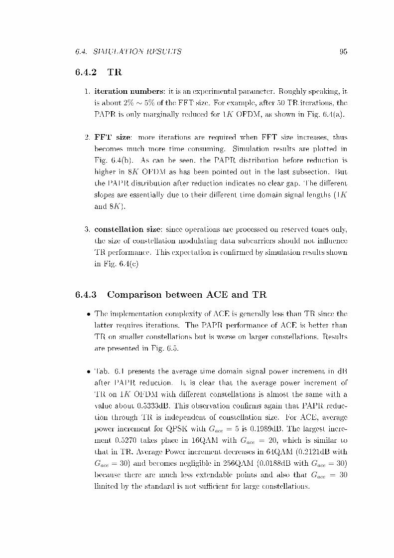
6.4. SIMULATION RESULTS 95
6.4.2 TR
1. iteration numbers: it is an experimental parameter. Roughly speaking, it
is about 2% ∼ 5% of the FFT size. For example, after 50 TR iterations, the
PAPR is only marginally reduced for 1K OFDM, as shown in Fig. 6.4(a).
2. FFT size: more iterations are required when FFT size increases, thus
becomes much more time consuming. Simulation results are plotted in
Fig. 6.4(b). As can be seen, the PAPR distribution before reduction is
higher in 8K OFDM as has been pointed out in the last subsection. But
the PAPR distribution after reduction indicates no clear gap. The di�erent
slopes are essentially due to their di�erent time domain signal lengths (1K
and 8K).
3. constellation size: since operations are processed on reserved tones only,
the size of constellation modulating data subcarriers should not in�uence
TR performance. This expectation is con�rmed by simulation results shown
in Fig. 6.4(c)
6.4.3 Comparison between ACE and TR
• The implementation complexity of ACE is generally less than TR since the
latter requires iterations. The PAPR performance of ACE is better than
TR on smaller constellations but is worse on larger constellations. Results
are presented in Fig. 6.5.
• Tab. 6.1 presents the average time domain signal power increment in dB
after PAPR reduction. It is clear that the average power increment of
TR on 1K OFDM with di�erent constellations is almost the same with a
value about 0.5333dB. This observation con�rms again that PAPR reduc-
tion through TR is independent of constellation size. For ACE, average
power increment for QPSK with Gace = 5 is 0.1989dB. The largest incre-
ment 0.5270 takes place in 16QAM with Gace = 20, which is similar to
that in TR. Average Power increment decreases in 64QAM (0.2121dB with
Gace = 30) and becomes negligible in 256QAM (0.0188dB with Gace = 30)
because there are much less extendable points and also that Gace = 30
limited by the standard is not su�cient for large constellations.

96CHAPTER 6. PEAK-TO-AVERAGE POWERRATIO (PAPR) REDUCTION
4 5 6 7 8 9 10 11 12 13 1410
−6
10−5
10−4
10−3
10−2
10−1
100
PAPR0
Pro
b.()
PA
PR
>P
AP
R 0)
1K OFDM originalQPSK ACE16QAM ACE64QAM ACE256QAM ACEQPSK TR16QAM TR64QAM TR256QAM TR
Figure 6.5: PAPR reduction performance comparison between ACE and TR
QPSK 16QAM 64QAM 256QAM
ACE 0.1989 0.5270 0.2121 0.0188
TR 0.5347 0.5336 0.5333 0.5333
Table 6.1: Average power increment on 1K time domain OFDM symbol modulated
by di�erent constellations after PAPR reduction

6.5. CONCLUSION 97
6.5 Conclusion
In this chapter, we studied two PAPR reduction methods, ACE and TR, both
analytically and experimentally. Special attention was paid to the impact of
parameters, such as constellation size and FFT size, on the PAPR reduction
performance. Simulation results revealed that constellation size dominates the
performance of ACE, while cancelation gain Gace should be carefully chosen to
avoid performance degradation. Lager extension threshold Lace improves the
performance but power consumption should be taken into account. The per-
formance of TR method is insensitive to constellation size and FFT size, but
iteration number increases proportionally to FFT size, indicating increment in
system complexity and time consumption.
Considering both PAPR reduction performance and average power increment
of the time domain signal, we conclude that ACE is better than TR in lower con-
stellations such as QPSK and 16QAM. On the other hand, TR outperforms ACE
in higher constellations at a price of higher power consumption and computational
load.

98CHAPTER 6. PEAK-TO-AVERAGE POWERRATIO (PAPR) REDUCTION

Chapter 7
System Simulation
The performance of individual modules of physical layer DVB-T2 transceiver has
already been investigated in the former chapters. This chapter will focus on
the performance of the transceiver as a whole. BICM, frame mapper and OFDM
modulator modules, along with their modules in the receiver side, are all included.
In order to verify our transceiver system, we set the same system parameters and
assumptions as reported in the o�cial implementation guidelines [11] and then
compare the end-to-end BER performance of our system with those provided in
the guidelines. BER performance is de�ned as the minimum SNR value under
which the receiver provides a BER less than 10−7 after LDPC decoding, corre-
sponding to BER of 10−11 after BCH decoding [11].
7.1 System Parameters and Assumptions
7.1.1 System Parameters
System parameters are summarized in Tab. 7.1.
In OFDM module, an 8K baseband OFDM system without subcarrier exten-
sion is applied. The length of cyclic pre�x is Ng = 256. Channel types considered
in the guidelines are AWGN channel, multipath Ricean fading channel, multipath
Rayleigh fading channel, and 0dB echo channel. Because we are more interested
in DVB-T2 performance in the mobile environment, 0dB echo channel is replaced
by TU-6 mobile channel in our simulations.
In frame mapper module, a random permutation on data cells replaces cell
and time interleaving as we have explained in Chap. 2. Pilot pattern is PP2 as
de�ned in Tab. 2.2.
99

100 CHAPTER 7. SYSTEM SIMULATION
Parameter Value
FFT size N 8192
Cyclic pre�x length Ng 256
Elementary time T 7/64µs
Pilot pattern PP2
Doppler frequency shift 50Hz (for mobile channel only)
Constellationsrotated + Q-delayed
QPSK, {16,64,256}QAM
LDPC code rate 1/2,3/5,2/3,3/4
LDPC codeword length Nldpc 64800
LDPC maximum decoding iteration 50
Table 7.1: Parameters of simulated DVB-T2 system
In BICM module, rotated and Q-delayed constellations are applied. LDPC
maximum decoding iteration number is 50.
7.1.2 Assumptions
Some strong assumptions are applied to the simulations to reveal the optimum
performance of DVB-T2. The a priori LLR information fed-back from LDPC
decoder to the demapper is replaced by genie-aided perfect a priori LLR [11].
This helps us to investigate the best performance that iterative demapping and
decoding is able to approach, being the same as our treatment on simulations of
BICM receiver in Sec. 3.3.5. Both synchronization and channel estimation are
assumed to be perfect [11] to prevent performance variation due to the use of
di�erent synchronization and channel estimation schemes. Under these assump-
tions, P1 and P2 preamble symbols are ignored and thus only normal OFDM
symbols are generated.
As a start point, pilots are not boosted in the frame mapper. Pilots thus
have the same power as the average power of data cells. Hence, the overall
system SNR, which is the carrier-to-noise ratio of all the modulated subcarriers
(C/N0), equals the carrier-to-noise ratio of subcarriers modulated by data cells
(C0/N0), where C is the average power of modulated subcarriers, C0 is the average
power of modulated data subcarriers, and N0 is the noise variance of complex
AWGN. Such simulations provide raw SNR values con�rmed by one or multiple
implementations [11]. These raw SNR values, denoted by γ0, are exactly the

7.2. SIMULATION RESULTS 101
minimum C0/N0 for the received data cells to reach the target BER performance
after receiver process.
In the next step, pilots are boosted according to the standard. Consequently,
system SNR C/N0 is larger than C0/N0. In order to guarantee C0/N0 > γ0
to achieve the target BER performance, C/N0 should be larger than γ0. The
di�erence between system SNR C/N0 and γ0 is the SNR penalty ∆bp due to pilot
boosting. This penalty can be easily calculated taking the number and power of
pilots into account as [11]:
∆bp = 10 log10
[Ndata +Nnb +Nsp · A2
sp +Ncp · A2cp
Ndata +Nnb +Nsp +Ncp
](7.1)
where Ndata, Nnb, Nsp, Ncp are the number of data subcarriers, non-boosted pilots,
scatter pilots and continual pilots, respectively. Asp and Acp are the amplitude
of scatted pilots and continual pilots, respectively [11]. A complete table of ∆bp
for every combination of FFT size and pilot pattern can be found in Tab. 46 of
the guidelines [11]. Particularly, ∆bp is 0.39dB for 8K OFDM without subcarrier
extension and with pilot pattern PP2 applied in our system.
In the �nal stage, time-frequency-direction linear interpolation we have men-
tioned in Sec. 4.4.3 are applied instead of perfect channel estimation according
to the guidelines [11]. The use of real channel estimation introduces a further
SNR loss. Although there is no mathematical approach to calculate this penalty
value, the guidelines have carried out some approximate values as a reference
based on some assumptions. Interested readers are referred to Clause. 14.4 of
[11]. Particularly, for pilot pattern PP2, the SNR penalty ranges from 0dB to
2.5dB for di�erent subcarrier locations.
The SNR penalty values of both pilot boosting and the use of real channel
estimation will be evaluated through our extensive computer simulations in the
next section.
7.2 Simulation Results
In our simulations, minimum SNR step is 0.1dB and thus is our SNR resolution.
To obtain reliable results, 50 erroneous decoded LDPC blocks are gathered for
each SNR point.

102 CHAPTER 7. SYSTEM SIMULATION
7.2.1 Perfect Channel Estimation without Pilot Boosting
Simulated system SNR requirements without pilot boosting and with perfect
channel estimation are given in Tab. 7.2. We also provide their di�erences com-
pared with the SNR values given in Tab. 44 of the guidelines [11].
By examining the di�erences we can make three observations:
1. in AWGN channel, our system provides SNR results exactly the same as
those given in the guidelines;
2. in Ricean fading channel, the performance degradation (i.e., requiring higher
SNR values to achieve the target BER) is 0.1dB due to our simpli�ed chan-
nel model.
3. in Rayleigh fading channel there is also performance degradation due to
our simpli�ed channel model. Its value is slightly larger than in Ricean
fading channel. It monotonically increases from 0.2dB to 0.4dB with larger
constellation size and LDPC code rate.
Consequently, we can say that our baseband physical layer DVB-T2 system well
represents the realistic one. The performance degradation in multipath channels
is due to the mismatch between our simpli�ed baseband channel models and the
passband ones. But the degradation is not signi�cant. The largest degradation
is 0.4dB taking place in Rayleigh fading channel with rate 3/4 LDPC code and
256QAM, where the standard SNR requirement is 22.6dB, being much larger
than 0.4dB.
A cross comparison among SNR requirements under di�erent channel types
reveals that:
• compared with SNR requirements in AWGN channel, the SNR degradation
due to Ricean fading channel is small. It increases from 0.3dB to 0.4dB
with larger constellation size and LDPC code rate;
• the SNR degradation due to Rayleigh fading channel shows the same ten-
dency but with much larger values. The SNR degradation with QPSK and
rate 1/2 LDPC code is only 0.9dB and it rises to as large as 2.6dB with
256QAM and rate 3/4 LDPC code;
• TU-6 mobile channel causes further SNR degradation ranging from 1dB to
1.3dB compared with those SNR requirements in Rayleigh fading channel.

7.2. SIMULATION RESULTS 103
Constellation Code rate AWGN Ricean Rayleigh Mobile
QPSK 1/2 1.0 [0.0] 1.3 [0.1] 2.2 [0.2] 3.5
16QAM 3/5 7.6 [0.0] 7.9 [0.1] 9.6 [0.3] 10.7
64QAM 2/3 13.5 [0.0] 13.9 [0.1] 15.9 [0.3] 16.9
256QAM 3/4 20.0 [0.0] 20.4 [0.1] 23.0 [0.4] 24.2
Table 7.2: Required SNR (dB) to achieve a BER=10−7 after LDPC decoding of various
constellation sizes and LDPC codes under the condition of perfect channel estimation
and without pilot boosting. (Bracketed values are the di�erence between simulation
results and the values reported in the implementation guidelines)
Constellation Code rate AWGN Ricean Rayleigh Mobile
QPSK 1/2 1.4 [0.4] 1.7 [0.4] 2.6 [0.4] 3.9 [0.4]
16QAM 3/5 8.0 [0.4] 8.3 [0.4] 10.0 [0.4] 11.1 [0.4]
64QAM 2/3 13.9 [0.4] 14.3 [0.4] 16.3 [0.4] 17.3 [0.4]
256QAM 3/4 20.4 [0.4] 20.8 [0.4] 23.4 [0.4] 24.6 [0.4]
Table 7.3: Required SNR to achieve a BER=10−7 after LDPC decoding of various
constellation sizes and LDPC codes under the condition of perfect channel estimation
and with pilot boosting. (Bracketed values are the SNR increment due to pilot boosting
compared with Tab. 7.2)
7.2.2 Perfect Channel Estimation with Pilot Boosting
Theoretical SNR penalty values ∆bp have already been carried out in Sec. 7.1.2.
In this subsection, we evaluate it through simulations where pilots are boosted
and channel estimation is assumed to be perfect. The theoretical penalty ∆bp
for 8K normal OFDM and pilot pattern PP2 is 0.39dB regardless constellation
sizes and LDPC types. Our simulation results in Tab. 7.3 state that this value
is 0.4dB for all combinations of constellation sizes and LDPC types. The 0.01dB
di�erence is due to our simulated SNR resolution (0.1dB). Consequently, we can
conclude that our simulation results strongly supports the theoretical value.
7.2.3 Realistic Channel Estimation with Pilot Boosting
Simulations in this subsection employ time-frequency-direction linear interpola-
tion and the results are given in Tab. 7.4. For pilot pattern PP2 where Dx = 6
Dy = 2, the SNR penalty ranges from 0dB to 2.5dB depending on subcarrier
locations. But the guidelines have not suggest the SNR degradation averaging

104 CHAPTER 7. SYSTEM SIMULATION
Constellation Code rate AWGN Ricean Rayleigh Mobile
QPSK 1/2 2.8 [1.4] 3.1 [1.4] 4.3 [1.7] 5.3 [1.4]
16QAM 3/5 9.2 [1.2] 9.5 [1.2] 11.6 [1.6] 12.8 [1.7]
64QAM 2/3 15.1 [1.2] 15.5 [1.2] 17.7 [1.4] 18.8 [1.5]
256QAM 3/4 21.5 [1.1] 22.0 [1.2] 24.8 [1.4] 26.1 [1.5]
Table 7.4: Required SNR to achieve a BER=10−7 after LDPC decoding of various
constellation sizes and LDPC codes under the condition of real channel estimation and
with pilot boosting. (Bracketed values are the SNR increment due to real channel
estimation compared with Tab. 7.3)
over all the subcarriers.
In our simulations, the average SNR degradation due to realistic channel es-
timation ranges from 1.1dB to 1.7dB. From Tab. 7.4, we can observe a general
tendency that SNR penalty increases with time-varying and frequency-selective
channels. Time-varying channels mainly a�ect time-direction interpolation. The
�uctuation of frequency domain channel transfer function, which is known as
frequency-selectivity, adversely in�uences frequency-direction interpolation. In
AWGN and Ricean fading channels, the frequency domain channels are �atter
than those in Rayleigh fading and mobile channels (refer to Fig. 2.5(b), Fig.
2.6(b) and Fig. 2.7(b) in Chap. 2, respectively). With less time-varying and
frequency-selectivity of channels, the linear interpolation algorithm can provide
better channel estimation performance and thus less SNR penalty.
7.3 Conclusion
In this chapter, we have simulated our baseband DVB-T2 system in regard to
its end-to-end BER performance and SNR requirements. We have used the same
system parameters and assumptions as those de�ned in the o�cial guidelines.
Simulated SNR requirements in AWGN channel are exactly the same as those in
the guidelines. This con�rmed the correctness of our baseband transceiver. We
have observed performance variation due to simpli�ed multipath channel models
but the variation is marginal. We have also con�rmed the SNR penalties due to
pilot boosting and realistic channel estimation.

Chapter 8
Conclusion and Future Work
In this thesis we have thoroughly studied the physical layer of DVB-T2 transceiver
system, including BICM, frame mapper and OFDM modules. We have designed
highly e�cient implementation methods for the transmitter side and have devel-
oped new techniques for optimum receiver. We have established a complete base-
band DVB-T2 system to facilitate our study and we have con�rmed its correctness
through extensive simulations on its end-to-end BER and SNR performance and
comparing the results with those provided in o�cial guidelines.
For BICMmodule, we have �rst discussed the properties and encoding/decoding
processes of BCH and LDPC codes. We have proposed e�cient BCH encod-
ing/decoding algorithms and an LDPC encoding algorithm. Simulations have
shown that BCH codes are quasi-error free codes with �xed bit-error-correcting
ability and LDPC codes are near Shannon-limit codes if we use soft decoding. We
then have investigated bit-interleaving and rotated constellation techniques which
o�er both code diversity and robustness to fading channels. We have designed a
low-complexity demapping algorithm for rotated constellation demapping.
For frame mapper module, we have carefully examined the structure of DVB-
T2 frames. To avoid cross-frame cell and time interleaving, we used random cell
interleaving within one T2 frame to guarantee independent fading of cells.
For OFDM module, we have �rst reviewed and modeled the impact of im-
perfect channel and receiver. We then have reviewed and compared existing
synchronization techniques in the literature, which deal with imperfect receiver.
For imperfect channel, we have reviewed several current channel estimation tech-
niques and have proposed a novel channel estimation technique called domain-
transform least-squares. It is insensitive to timing synchronization errors and
Doppler frequency shifts. It provides competitive BER performance with current
105

106 CHAPTER 8. CONCLUSION AND FUTURE WORK
channel estimation methods but with a much lower complexity.
In OFDM module, a P1 preamble symbol is transmitted before each frame of
P2 and normal symbols. We have thoroughly studied the structure and proper-
ties of P1 symbol and proposed new time domain synchronization and decoding
methods for it. Not only it avoids post-FFT decoding, but it also provides very
good synchronization performance and decoding SNR gain compared with the
performance reported in the o�cial guidelines. We have introduced two new
concepts in this method, which can be adapted for the synchronization of other
OFDM symbols.
We have also studied OFDM PAPR reduction techniques employed in DVB-
T2, including ACE and TR. We have reviewed general ACE and TR algorithms
and demonstrated modi�cations for DVB-T2. We have done simulations to eval-
uate their performance. The results show that ACE outperforms TR in smaller
constellations but TR performs better in larger constellations at a cost of higher
power consumption and processing delay. We have also recommended optimal
choices of parameters based on simulations.
As the last step, we have investigated the end-to-end BER performance and
the minimum SNR values to achieve a BER of 10−7 after LDPC decoding of
our complete baseband DVB-T2 system. We have applied the same system pa-
rameters and assumptions as de�ned in the o�cial guidelines. The consistency
between our results and those in the guidelines veri�ed the correctness of our
baseband transceiver and revealed the performance degradation due to simpli-
�ed baseband channel models. Our simulation results have also con�rmed the
theoretically calculated SNR penalty due to pilot boosting and realistic channel
estimation.
Although we have not simulated P2 OFDM symbols de�ned in DVB-T2, the
di�erence between them and normal OFDM symbols are not signi�cant. We have
already emphasized the adaption of algorithms for normal OFDM symbols to P2
OFDM symbols.
In the future, we will develop a user-graphic-interface under Matlab envi-
ronment for our DVB-T2 system. Our research interest will then turn to other
layers of broadcasting and other DVB stands such as DVB for hand-held (DVB-
H) [41] and DVB for satellite (DVB-S2) [42], in which new techniques other than
in DVB-T2 are adopted to enhance broadcasting performance. For example, in
DVB-S2 a variable coding and modulation (VCM) scheme is used, allowing opti-
mizing bandwidth utilization by dynamically changing transmission parameters.
16- and 32- amplitude and phase-shift keying (APSK) modulations are used in

107
DVB-S2, which is better than QAM in terms of lower number of possible am-
plitude levels, resulting in fewer problems with non-linear ampli�ers. In DVB-H
where reducing hand-held receiver power consumption is critical, a time-slicing
technique is employed where data are sliced into bursts and the front end of the
receiver switches on only for the time interval when the data burst of a selected
service is on air. These new techniques motivate research on their receiving tech-
niques.

108 CHAPTER 8. CONCLUSION AND FUTURE WORK

Bibliography
[1] ETSI EN 300 744, �Digital Video Broadcasting (DVB); Framing structure,
channel coding and modulation for digital terrestrial television,� .
[2] DVB Document A122, �Frame structure, channel coding and modulation for
a second generation digital terrestrial television broadcasting system (DVB-
T2),� June 2008.
[3] L. Vangelista, N. Benvenuto, C. Nokes S. Tomasin, J. Stott, A. Filippi,
M. Vlot, V. Mignone, and A. Morello, �Key technologies for next-generation
terrestrial digital television standard DVB-T2,� IEEE Commun. Magazine,
pp. 146�153, Oct. 2009.
[4] S. Lin and D. J. Costello, �Error control coding,� Upper Saddle River, N.J.
: Pearson-Prentice Hall, 2004.
[5] R. G. Gallager, �Low density parity check codes,� Monograph, M.I.T. Press,
1963.
[6] J. Boutros and E. Viterbo, �Signal space diversity: a power- and bandwidth-
e�cicient diversity technique for the Rayleigh fading channel,� IEEE Trans.
on Informaiton Theory, vol. 44, pp. 1453�1467, July 1998.
[7] C. A. Nour and C. Douillard, �Rotated QAM constellations to improve
BICM performance for DVB-T2,� IEEE ISSSTA 08, pp. 354�359, 2008.
[8] B. Krongold and D. L. Jones, �PAR reduction OFDM via active constellation
extension,� IEEE Trans. on Broadcasting, vol. 49, pp. 258�268, Sep 2005.
[9] S. H. Han and J. H. Lee, �An overview of peak-to-average power ratio
reduction techniques for multicarrier transmission,� IEEE Trans. on Wireless
Commun., vol. 12, pp. 56�65, 2005.
109

110 BIBLIOGRAPHY
[10] J. Chen and C. Li, �Tone reservation using near-optimal peak reduction tone
set selection algorithm for PAPR reduction in OFDM systems,� IEEE Signal
Processing Letters, vol. 17, pp. 933�936, Nov 2010.
[11] DVB Document A133, �Implementation guidelines for a second generation
digital terrestrial television broadcasting system (DVB-T2),� June 2010.
[12] M. Speth, S. Fechtel, G. Fock, and H. Meyr, �Optimum receiver design for
wireless broadband system using OFDM-part I,� IEEE Trans. on Commun.,
vol. 47, no. 11, pp. 1668�1677, Nov. 1999.
[13] M. Speth, S. Fechtel, G. Fock, and H. Meyr, �Optimum receiver design for
OFDM-based broadband tramsmisson-part II: A case study,� IEEE Trans.
on Commun., vol. 49, no. 4, pp. 571�578, April 2001.
[14] H. Minn, V. K. Bhargava, and K. B. Letaief, �A robust timing and frequency
synchronization for OFDM systems,� IEEE Trans. on Wireless Commun.,
vol. 2, no. 4, pp. 822�839, July 2003.
[15] A. Viessmann, C. Kocks, A. Waadt. C. Spiegel, J. Kim, Y. Lim, and
H. Lee, �An implementation-friendly synchronization algorithm for multi-
media HDTV receivers,� in ISABEL 2009, 2009.
[16] L.Vangelista and M. Rotoloni, �On the analysis of P1 symbol performance
for DVB-T2,� in IEEE Sarno� Symposium'09, April 2009.
[17] M. Rotoloni, S. Tomansin, and L. Vangelista, �On correlation-based synchro-
nization for DVB-T2,� IEEE Commun. Letters, vol. 14, no. 3, pp. 248�250,
March 2010.
[18] E. Zehavi, �8-PSK trellis codes for a Rayleigh channel,� IEEE Trans. on
Commun., vol. 40, pp. 873�884, May 1992.
[19] G. Caire, G. Taricco, and E. Biglieri, �Bit-interleaved coded modulaton,�
IEEE Trans. on Information Theory, vol. 44, no. 3, pp. 927�946, May 1998.
[20] S. T. Brink, J. Speidel, and R. Yan, �Iterative demapping and decoding for
multilevel modulation,� IEEE GLOBECOM 98, vol. 1, pp. 579�584, 1998.
[21] E. Telatar, �Capacity of multi-antenna Gaussian chanels,� Eur. Trans. on
Telecommun., vol. 10, pp. 583�596, Nov 1999.

BIBLIOGRAPHY 111
[22] S. M. Alamouti, �A simple transmit diversity technique for wireless commu-
nications,� IEEE Journal on Select Areas in Commun., vol. 16, pp. 1458,
Oct 2010.
[23] M. Yu and P. Sadeghi, �Time domain synchronization and decoding of P1
symbol in DVB-T2,� ICASSP 2011, pp. 3520 � 3523, May 2011.
[24] J. G. Prokais, �Digital communications,� McGraw-Hill Book Corp., Singa-
pore, ISBN: 0071138145, 1995.
[25] J. L. Massey, �Shift-register synthesis and BCH decoding,� IEEE Trans. on
Information Theory, vol. 15, no. 1, July 1969.
[26] D. J. Costello, �An introduction to low-density parity check codes,� Univer-
sity of Notre Dame, August, 2009.
[27] D. Yuan and H. Zhang, �LDPC code, principles and applications,� China
Post & Telecom Press, 2008.
[28] X. Wang, Y. Wu, and J. Chouinard, �A channel characterization technique
using frequency domian pilot time domain correlation method for DVB-T
systems,� IEEE Trans. on Consumer Electronics, vol. 49, no. 4, pp. 949�
957, Nov. 2003.
[29] B. Jahan, M. Lanoiselee, G. Degolet, and R. Rabineau, �Frame synchroniza-
tion method for OFDM/OWAM and OFDM/QAM modulation,� in IEEE
Int. Conf. on Circuit and Systems for Commun., Shanghai, 2008, May 2008.
[30] O. Edfors, M. Sandell, J.-J. van de Beek, S. Wilson, and P. Borjesson,
�OFDM channel estimation by singular value decomposition,� IEEE trans.
on Commun., vol. 46, no. 7, pp. 931�939, July 1998.
[31] Y. (Geo�rey) Li, �Pilot-symbol-aided channel estimation for OFDM in wire-
less systems,� IEEE Trans. on Veh. Technol., vol. 49, no. 4, pp. 1207�1215,
July 2005.
[32] Y. Mosto�, D. C. Cox, and A. Bahai, �E�ect of frame synchronization
errors on pilot-aided channel estimation in OFDM: analysis and solution,�
in Proc. IEEE Int. Symp. on Wireless Personal Multimedia Commun., pp.
1309�1313, Oct. 2002.
112 BIBLIOGRAPHY
[33] M. Liang and D. C. Yang, �Channel impulse response order adjustment for
OFDM in SFN,� in 4th Int. Conf. WiCOM 2008, pp. 1�4, Oct. 2008.
[34] J. Lin, �Least-squares channel estimation for mobile OFDM communication
on time-varying frequency-selective fading channels,� IEEE Trans. on Veh.
Technol., vol. 57, no. 6, pp. 3538�3550, Nov. 2008.
[35] M. Hsieh and C. Wei, �Channel estimation for OFDM systems based on
comb-type pilot arrangement in frequency selective fading channels,� IEEE
Trans. on Consumer Electronics, vol. 44, pp. 217�225, Feb. 1998.
[36] M. T. Nair, �Linear operator equations: approximation and regularization,�
World Scienti�c Publishing, ISBN: 9812835644, 2009.
[37] P. C. Hansen, �Rank-de�cient and discrete ill-posed problems,� SIAM Pub-
lish, Philadelphia, USA, ISBN: 0898714036, 1998.
[38] A. Filippi and S. Serbetli, �OFDM symbol synchronization using frequency
domain pilots in time domain,� IEEE Trans. on wireless communi., vol. 8,
no. 6, pp. 3240�3248, June 2009.
[39] J. G. Doblado, V. Baena, A. C. Oria, D. P. Calderon, and P. Lopez, �Coarse
time synchronization for DVB-T2,� IEEE Electronics Letters, vol. 46, May
2010.
[40] F. Classen and H. Meyr, �Frequency synchronization algorithms for OFDM
systems suitable for communication over frequency selevtive fading chan-
nels,� in Proc. Veh. Technol. Conf., vol. 3, pp. 1655�1659, 1994.
[41] ESTN 302 304, �Digital Video Broadcasting (DVB); Transmission system
for handheld terminals (DVB-H),� Nov 2004.
[42] ESTN 302 307, �Digital Video Broadcasting (DVB); Second generation fram-
ing structure, channel coding and modulation systems for broadcasting, in-
teractive services, news gathering and other broadband satellite applications
(DVB-S2),� April 2009.