Embed Size (px)
Citation preview
A STUDY COMPARING CHANGES IN LOADING CONDITIONS
OF AN EXTENDED SERVICE LIFE AIRCRAFT
USING 17-7PH STAINLESS STEEL
by
Tony Clayton Hyer
A thesis submitted to the faculty of The University of Utah
in partial fulfillment of the requirements for the degree of
Master of Science
Department of Mechanical Engineering
The University o f Utah
August 2014

Copyright © Tony Clayton Hyer 2014
All Rights Reserved

The University of Utah Graduate School
STATEMENT OF THESIS APPROVAL
The thesis of _____________ Tony Clayton Hyer___________________
Has been approved by the following supervisory committee members:
_______________Ken J. Monson______________ , Chair 4/25/2014Date Approved
______________Mark L. Thomsen____________, Member 4/25/2014Date Approved
_______________K. Larry DeVries____________, Member 4/25/2014Date Approved
and by_______ Timothy A. Ameel_____________________ , Chair/Dean of
the Department/College/School o f_________ Mechanical Engineering________
and by David B. Kieda, Dean of The Graduate School.
ABSTRACT
Industry and the military are always looking for ways to stretch their dollar. One
way to do this is to make the equipment they currently own last longer in lieu of buying
new. For example, many of the aircraft in the USAF have gone beyond their expected
service life and over that time have experienced changes in usage. In order for the
USAF, or others in the aviation industry, to make their aircraft last longer, they must
understand how the changes in usage affect their aircraft.
The purpose of this study was to determine the sensitivity of a representative
stainless steel specimen to two different load spectra, spectrum A and spectrum B. This
was accomplished by conducting fatigue experiments, baselines for each spectrum and
three different combinations of the two spectra, performing fractographic examinations of
the fracture surfaces and developing computer simulations, using AFGROW, to represent
test data. The results showed that crack growth under spectrum B type loading
conditions was significantly slower than under spectrum A. The fractography showed
clear distinctions between the spectra fracture surfaces. Also, AFGROW simulations
were successful in replicating test data. These results emphasize the need for continual
monitoring of fatigue critical locations to better maintain aircraft.

I would like to dedicate this work to my wife Joni, our children Thomas, Lucy and Logan and to our future.
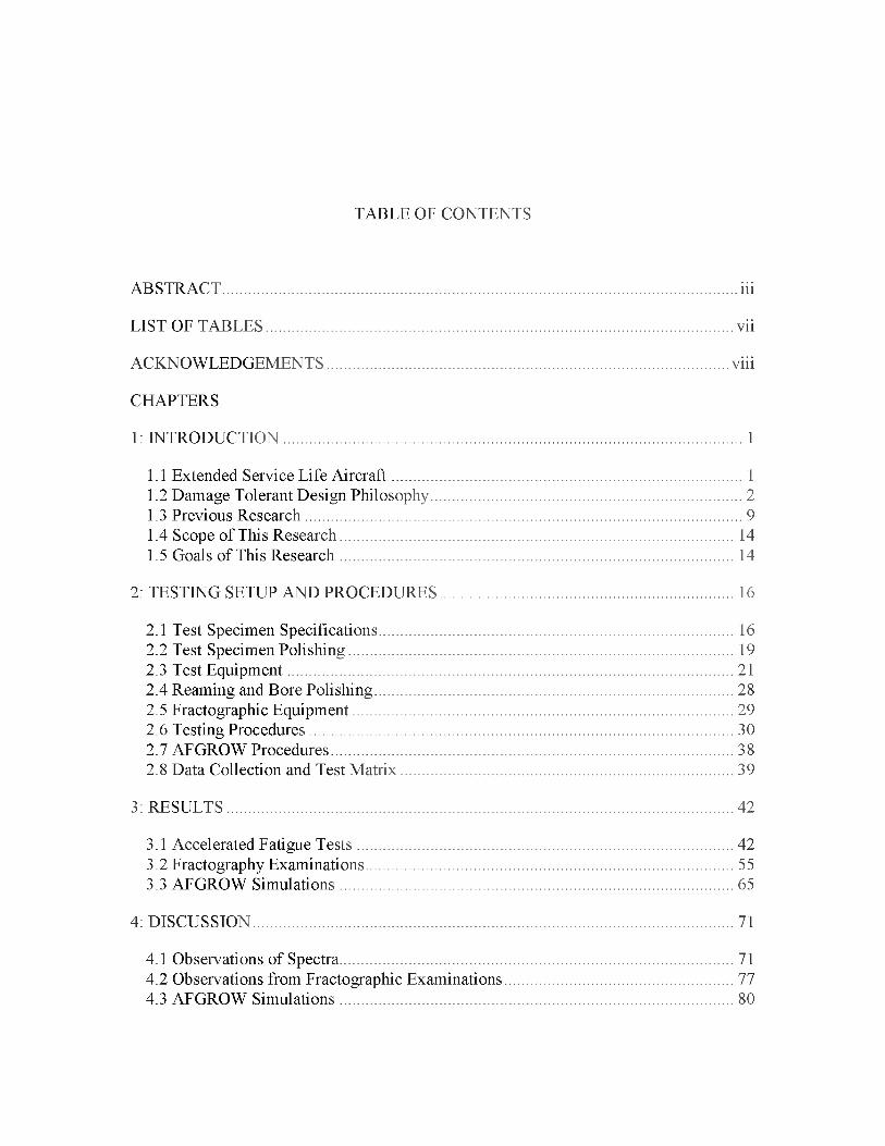
TABLE OF CONTENTS
ABSTRACT.................................................................................................................................iii
LIST OF TABLES.....................................................................................................................vii
ACKNOWLEDGEMENTS.................................................................................................... viii
CHAPTERS
1: INTRODUCTION.................................................................................................................. 1
1.1 Extended Service Life A ircraft....................................................................................... 11.2 Damage Tolerant Design Philosophy............................................................................. 21.3 Previous Research.............................................................................................................91.4 Scope of This Research.................................................................................................. 141.5 Goals of This Research.................................................................................................. 14
2: TESTING SETUP AND PROCEDURES.........................................................................16
2.1 Test Specimen Specifications........................................................................................ 162.2 Test Specimen Polishing................................................................................................192.3 Test Equipment............................................................................................................... 212.4 Reaming and Bore Polishing......................................................................................... 282.5 Fractographic Equipment...............................................................................................292.6 Testing Procedures..........................................................................................................302.7 AFGROW Procedures.................................................................................................... 382.8 Data Collection and Test M atrix...................................................................................39
3: RESULTS.............................................................................................................................. 42
3.1 Accelerated Fatigue T ests..............................................................................................423.2 Fractography Examinations............................................................................................553.3 AFGROW Simulations.................................................................................................. 65
4: DISCUSSION ........................................................................................................................ 71
4.1 Observations of Spectra.................................................................................................. 714.2 Observations from Fractographic Examinations.........................................................774.3 AFGROW Simulations.................................................................................................. 80

5: CONCLUSIONS AND RECOMMENDATIONS...........................................................85
5.1 Conclusions......................................................................................................................855.2 Recommendations...........................................................................................................87
APPENDICES
A: TEST SPECIMEN FABRICATION PROCEDURES AND MATERIAL CERTIFICATION SHEETS.................................................................................................... 90
B: POLISHING, REAMING AND SEM PROCEDURES...............................................101
C: SOUTHWEST RESEARCH INSTITUTE EQUIPMENT INFORMATION...........104
D: FATIGUE MACHINE AND LOAD CELL CALIBRATION CERTIFICATIONS 111
E: EXAMPLE OF PRECRACK CALCULATIONS.........................................................115
F: PROCEDURES FOR AFGROW ANALYSIS.............................................................. 119
G: CRACK GROWTH DATA SHEETS............................................................................ 122
H: ADDITIONAL CRACK GROWTH CURVES.............................................................149
I: ADDITIONAL SEM IMAGES OF TEST SPECIMEN FRACTURE SURFACES .. 155
REFERENCES........................................................................................................................167
vi
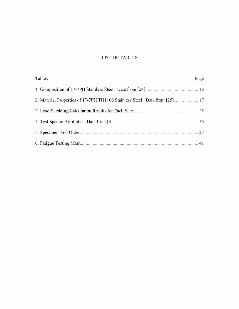
LIST OF TABLES
Tables Page
1: Composition of 17-7PH Stainless Steel. Data from [24]................................................16
2: Material Properties of 17-7PH TH1100 Stainless Steel. Data from [25].....................17
3: Load Shedding Calculation Results for Each Step...........................................................35
4: Test Spectra Attributes. Data from [8].............................................................................. 36
5: Specimen Test O rder............................................................................................................37
6: Fatigue Testing Matrix..........................................................................................................41
ACKNOWLEDGEMENTS
I feel a distinct need to give thanks to the many people who made this work
possible. The first thanks need to go to Dr. Mark Thomsen, Robert Pilarczyk, Scott
Carlson and Dallen Andrew who were the main players in procuring the specimens,
arranging lab time and giving continued guidance during this project. I very much
appreciate their willingness to work with me and give me this opportunity to get some
real, hands-on, experience in running a fatigue experiment. I also need to thank Dr. Ken
Monson and Dr. K. Larry DeVries who were also willing to work with me during this
project and help with its completion. Thanks need to go to Tom Slowick in the machine
shop at the University of Utah for allowing me to use the equipment there for a portion of
this project.
I need to thank those in the Engineering and Science Lab on Hill AFB, namely,
Wayne Patterson, Wes Finneran, Cody Hone and Scot Frew. These gentlemen went the
extra mile in working with me so that I could use the facilities and equipment in their lab
during a significant portion of this project. Without their assistance, this project would
have been extremely more difficult to complete.
I would like to thank Luciano “Lucky” Smith and Jim Feiger from Southwest
Research Institute. When the fatigue machine on Hill AFB went out of commission for a
time, these gentlemen made it possible to complete the fatigue testing of several test

specimens. I greatly appreciate their patience with the routine phone calls and answering
all the questions that I had.
I also have a deep appreciation for all the help and assistance offered to me by my
fellow student, Roger Beal. He and I spent many long hours figuring out what was going
to be necessary for every step of this project. He was very willing to counsel me and help
me find answers to most o f the questions that arose during this process.
I need to thank my supervisors, Ronald Montgomery, Chad Hogan and Brad
Martin in the Landing Gear Office at Hill AFB. These gentlemen were very willing and
supportive during my whole graduate school experience. They were constantly willing to
work with my schedule and accommodate my needs. A special thanks also goes to Dan
Christensen, Douglas Ball, Jared Butterfield and Jim Yerke, who were instrumental in
helping me to be admitted to the Palace Acquire program.
Lastly but most importantly, I need to thank my wife and children for the many
years o f support and love they have given to me. They were my motivation during all my
years of schooling. They are the reason I’ve accomplished as much as I have over these
past several years that they have been a part of my life.
ix

CHAPTER 1
INTRODUCTION
1.1 Extended Service Life Aircraft
Few players have as critical of a role in the defense strategy of the United States,
and many other countries for that matter, and world transportation as the aerospace
industry. Having said that, it is extremely expensive to buy and maintain aircraft.
According to Boeing’s website, a new 737 MAX 9 will cost a buyer upwards of $109.9
million in 2013 dollars. [1] A new 777-300ER will cost a buyer a staggering $320.2
million in 2013 dollars. [1] On the military side, the unit cost for just one F-16C/D
model is $18.8 million in 1998 dollars. [2] Those figures don’t even reflect the cost of
maintaining each of those aircraft. Due to the large amounts of money involved, industry
and the military look for ways to reduce cost.
When faced with the decision to buy expensive new aircraft or maintain what they
have, industry and the government often resort to the latter. Some examples of extended
service life aircraft can be seen in the United States military. The Air Force has extended
the service life of the A-10 Thunderbolt II and the B-52 Stratofortress, as just a couple of
examples. The A-10 had an initial service life of 6,000 hours and was due to retire in
Fiscal Year (FY) 2005. [3] The Air Force, after several upgrades, has now extended the
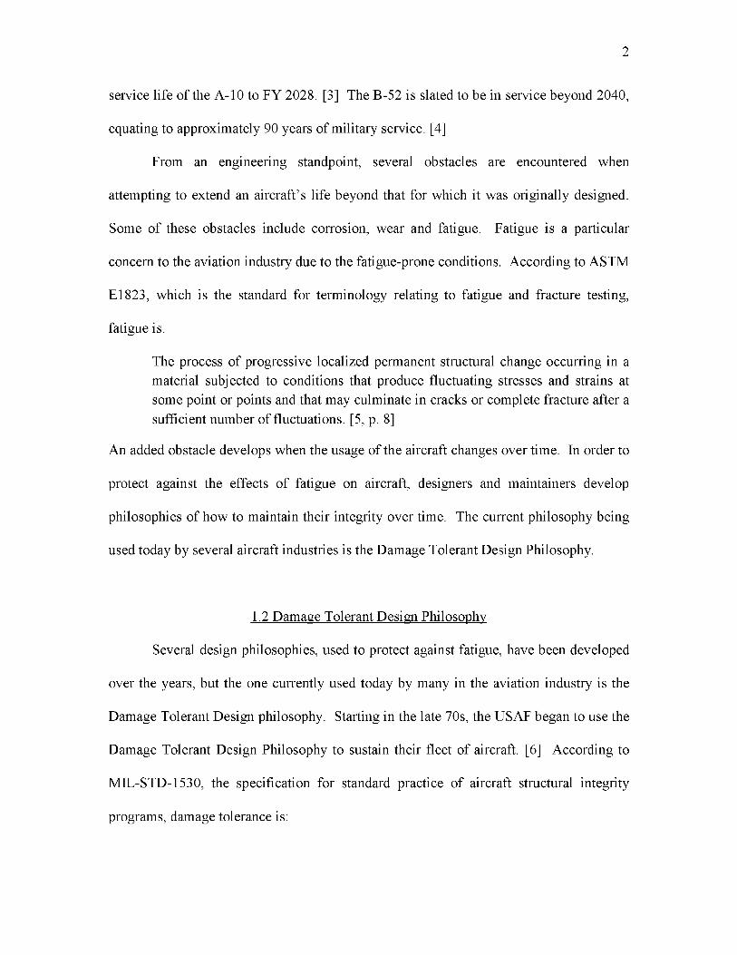
2
service life of the A-10 to FY 2028. [3] The B-52 is slated to be in service beyond 2040,
equating to approximately 90 years of military service. [4]
From an engineering standpoint, several obstacles are encountered when
attempting to extend an aircraft’s life beyond that for which it was originally designed.
Some of these obstacles include corrosion, wear and fatigue. Fatigue is a particular
concern to the aviation industry due to the fatigue-prone conditions. According to ASTM
E1823, which is the standard for terminology relating to fatigue and fracture testing,
fatigue is:
The process of progressive localized permanent structural change occurring in a material subjected to conditions that produce fluctuating stresses and strains at some point or points and that may culminate in cracks or complete fracture after a sufficient number of fluctuations. [5, p. 8]
An added obstacle develops when the usage of the aircraft changes over time. In order to
protect against the effects of fatigue on aircraft, designers and maintainers develop
philosophies of how to maintain their integrity over time. The current philosophy being
used today by several aircraft industries is the Damage Tolerant Design Philosophy.
1.2 Damage Tolerant Design Philosophy
Several design philosophies, used to protect against fatigue, have been developed
over the years, but the one currently used today by many in the aviation industry is the
Damage Tolerant Design philosophy. Starting in the late 70s, the USAF began to use the
Damage Tolerant Design Philosophy to sustain their fleet of aircraft. [6] According to
MIL-STD-1530, the specification for standard practice of aircraft structural integrity
programs, damage tolerance is:
3
the attribute of a structure that permits it to retain its required residual strength for a period of unrepaired usage after structure has sustained specific levels of fatigue, corrosion, accidental, and/or discrete source damage. [7, p. 5]
Damage tolerance relies heavily on fracture mechanics concepts, namely, fatigue crack
growth, residual strength as well as nondestructive inspections (NDI), to help manage the
remaining life in an aircraft’s structure.
Damage Tolerant Designs assume that initially, there is some discontinuity in a
given material, new or old, used in the aircraft’s structure. [6] Often these discontinuities
become origination sites for crack development. [6] It is the objective of the Damage
Tolerant Design concept to not allow these discontinuities to develop into cracks, by
means of fatigue, that reach a critical length resulting in unstable crack growth and
failure. [7] The following sections explain in greater detail the role of fatigue crack
growth, residual strength and NDI techniques in the Damage Tolerant Design philosophy.
1.2.1 Fatigue Crack Growth
As was mentioned previously, the Damage Tolerant Philosophy begins with
assuming that there exists some discontinuity in the material from which a crack may
developed when subjected to some type of loading. Records collected by the USAF have
shown that the primary reasons that cracks grow in their aircraft are due to fatigue, stress
corrosion and corrosion-fatigue mechanisms. [6] According to the USAF Damage
Tolerance Design Handbook, when referring to flaws in the aircraft structure:
The safety of the aircraft is dependent on their initial sizes, the rates of growth with service usage, the critical flaw sizes, the inspectability of the structure, and the fracture containment capabilities of the basic structural design. [6, p. 1.2.1]
This reference also states that:

4
it is essential that safety of flight be provided through the consideration of an “initial flaw” model in which some size of initial damage is assumed to exist consistent with the inspection capability either in the field or during manufacture. [6, p. 1.2.1]
Those models, to which the Damage Tolerant Handbook is referring, are developed
through a process of fatigue testing and developing crack growth simulations that
replicate the results of the tests.
Today, the aviation industry and the military develop fatigue life models using
crack growth modeling programs. An example of a crack growth modeling program that
the USAF uses is AFGROW. These programs can be used for a wide variety of
structures as they are typically not system, or aircraft, specific. The results from the tests
and analyses allow users to approximate crack growth rates and critical flaw sizes. These
data are then used to determine appropriate inspection intervals and the resulting
component life expectancy. Fig. 1 is an example of a plot displaying a typical crack
growth curve. In order to develop a model that can accurately predict what is actually
occurring on the aircraft, one must understand the loading conditions that are occurring
on the aircraft.
1.2.1.1 Load History
There are primarily two types of loading conditions used for fatigue tests. One
type of loading is known as constant amplitude loading. According to ASTM E1823,
constant amplitude loading is, “a loading (straining) in which all of the peak forces
(strains) are equal and all of the valley forces (strains) are equal.” [5, p. 4] This type of
loading is used often for developing material properties, but it is not appropriate for
characterizing how a material will behave on an aircraft due to the fact that the loading

5
TYPICAL CRACK GROWTH CURVE
Figure 1 Typical Fatigue Crack Growth Curve used for Damage Tolerance Analysis
conditions are not constant.
The other type of loading used in fatigue experiments is known as spectrum
loading, variable amplitude loading or irregular loading. [5] The ASTM E1823 definition
for spectrum loading simply states that it is, “a force-time program consisting of some (or
all) unequal peak and valley forces.” [5, p. 16] If one can obtain the load history of a
location on an aircraft, a loading spectrum can be developed. These data are then entered
into a fatigue machine program and used to run an accelerated fatigue test. The results o f
these tests, if done correctly, will give a more accurate representation than the constant
amplitude test of how a material will perform on an aircraft, or any other product for that
matter.

1.2.1.2 Aircraft Spectrum Development
Different methodologies can be used to obtain loading data for different locations
on an aircraft. The type of measurement method used will be determined by the loading
conditions. The fatigue testing conducted for this study used measurements from the
Individual Aircraft Tracking Program (IATP) for military aircraft. [8] This program
recorded acceleration changes while the aircraft were in flight using a counting
accelerometer. [9] Those changes in acceleration can be used to derive loading
conditions at various points in the aircraft. The point chosen for this study was picked
due to the severity of the loading conditions and the fact that the material in that location
is 17-7PH stainless steel, about which little data has been gathered for this particular
aircraft. One of the desired outcomes of this study was to determine how the stainless
steel material would behave under the two spectra. A similar study, performed in
conjunction with this one, was also conducted using 2024-T351 aluminum. [10]
The data obtained from the IATP system were converted into loads compiled,
using a methodology called cycle counting in such a manner that showed the number of
times load levels were exceeded during a given period of time. An example of an
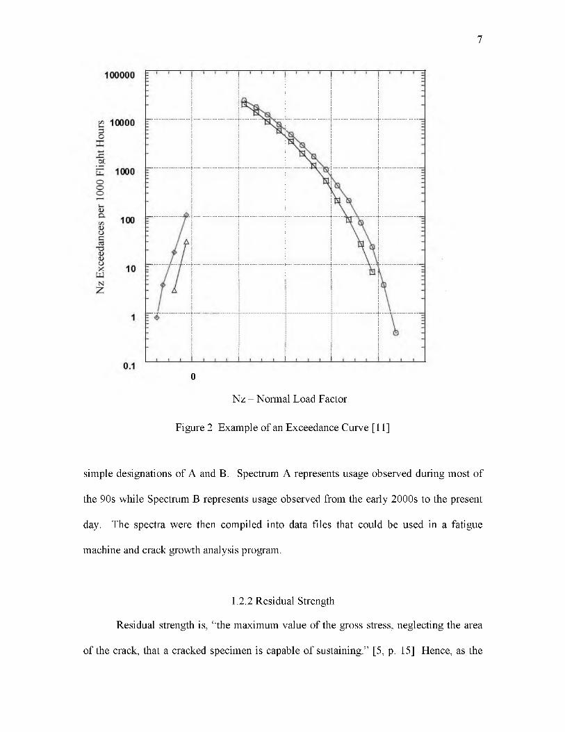
exceedance curve, which is a graphical representation of loads and occurrences, is shown
in Fig. 2. Once its known how many times different loads should be represented in the
spectrum, a randomized base-peak-base sequence of loads is developed.
Over the years that the IATP system had been in use, it was noticed that the usage
of the aircraft had changed significantly. With this new information, it was determined
that several spectra would need to be developed to represent the different usage periods.
For the purposes of this study, two different spectra were compared and were given the
6
7
0
Nz - Normal Load Factor
Figure 2 Example of an Exceedance Curve [11]
simple designations of A and B. Spectrum A represents usage observed during most of
the 90s while Spectrum B represents usage observed from the early 2000s to the present
day. The spectra were then compiled into data files that could be used in a fatigue
machine and crack growth analysis program.
1.2.2 Residual Strength
Residual strength is, “the maximum value of the gross stress, neglecting the area
of the crack, that a cracked specimen is capable of sustaining.” [5, p. 15] Hence, as the

crack increases in length, the residual strength of the specimen decreases. The residual
strength of the specimen can be determined using Linear Elastic Fracture Mechanics
(LEFM).
Beginning in the 19th century, with the advent of the Industrial Revolution, a
dramatic increase in the use of metals for structural purposes occurred. [12] With the
dramatic increase in metal usage, there came an increase in the number of failures due to
fracture. In 1920, a researcher by the name of Alan Arnold Giffith came up with a
successful method to analyze crack propagation in brittle structures, i.e., glass. [12] His
research involved relating the elastic strain energy with the surface energy of a system.
In other words, he determined that crack extension occurs when the elastic strain energy
available is larger than the available surface energy. [12] This research, which Griffith
developed, became the foundation for future Fracture Mechanics studies. In the late
1940s, Irwin suggested that, “the Griffith theory for ideally brittle materials could be
modified and applied to both brittle materials and metals that exhibit plastic
deformation.” [12, p. 12] Similar to Griffiths approach, Irwin recognized that, “a
material’s resistance to crack extension is determined by the sum of the surface energy
and the plastic strain work.” [12, p. 12] Irwin’s approach is now known as stress
intensity and is given by the following equation. [12]
K = a ^ n a fi
K is the stress intensity factor, o is the far field stress, a is the crack length and P is the
geometry correction factor. This equation suggests that crack extension will occur when
K is at a critical value. [12] In order to use the stress intensity approach, one must know
8

9
if a crack is present and its size in the structure. Today, NDI methods are used to help
make those determinations.
1.2.3 Nondestructive Inspections
As was mentioned previously, it is assumed that all materials have some
discontinuity in them that can eventually produce a crack by means of fatigue. Thus,
those in the aviation industry on a routine basis inspect aircraft on a predetermined
interval to assess if any damage is detectable and to what extent. In order to save money,
these inspection methods need to leave the component intact so that it can be reused or
repaired, if the damage is not too severe. Some typical types of inspections that are used
today are liquid penetrants, eddy current, x-ray and ultrasonic. If damage is detected
using one of these NDI methods, the remaining life can be determined from fatigue crack
growth data generated for that specific component.
1.3 Previous Research
As was explained earlier, the beginnings of fracture mechanics began in the
1920s. In the time since then, it has been observed that crack growth behavior is
dependent on several factors, such as material properties, type of structure, environmental
conditions and loading conditions. [13] The one factor of particular interest in this study
is the effect of loading conditions. Many tests over the years have been conducted to
better understand how overloads and underloads affect the fatigue life of a component.
1.3.1 Overload and Underload Affects
In constant amplitude loading, the max and min loads remain constant over the
duration of the test. The simplest form of an overload event occurs when at least one
cycle exceeds the typical max value of a constant amplitude test. One would probably at
first conclude that such an event would decrease the fatigue life of the item when in
reality, the opposite is usually true. This phenomenon is referred to as retardation of the
crack growth rate.
In an article written by P.J. Bernard, T. C. Lindley and C.E. Richards, they
reported on experiments of two types of steel, Ducol W30B and FV520B. [14] The main
differences between the two materials were yield strength and strain hardening. [14]
Ducol has a yield strength of 366 MNm" (53.1 ksi) and a percent elongation of 38 while
FV520B has a yield strength of 940 MNm-2 (136.3 ksi) and a percent elongation of 20.
[14] The results of the tests showed that FV520B experienced a sharp decrease in the
crack growth rate immediately following the overload. [14] Ducol also experienced a
decrease in the crack growth rate following the overload event with the difference being
that the transition to the slower rate was more gradual. [14] In both cases, the crack
continued to grow at the slower rate for a period of time then reverted back to the original
crack growth rates. [14] It was also observed that in order for the overload to have any
effect on the fatigue life, it had to exceed a limit, which the authors determined to be in
the range of a 40 to 60 percent load increase. [14]
Another article by W.X. Alzos, A.C. Skat, Jr. and B.M. Hillberry reported on the
effects of overloads preceded and followed by underloads. [15] The material used in
these experiments was 2024-T3 aluminum. [15] The tests were conducted such that the
underload followed the overload at varying stress ratios of overload and underload
10
events. These tests showed that the more negative the stress ratio, the greater the
reduction of the retardation effect. [15] This same study also showed that when the
underload preceded the overload, the result was the same as a test conducted with only
overloads. [15] Similar results were seen in a study conducted by R.I Stephens, D.K.
Chen and B.W. Hom. [16] Over the years, it has been observed that in order to more
accurately determine how a material will behave under real life conditions, methods had
to be developed to study more complex loading conditions.
1.3.2 Variable Amplitude Load Affects
With the aid of computer-controlled fatigue testing, researchers have been able to
test materials using complex loading scenarios that represent actual operational
conditions. In a study by J.A. Reiman, M.A. Landy and M.P. Kaplan, they conducted
tests using several different types of loading to determine the effect on fatigue life. [17]
The results of the study showed that spectrum or flight-by-flight type loading conditions
were more accurate in representing field data than previous methods relying on constant
amplitude data. [17]. Similar results were also seen in a study by W. Zhuang, S. Barter
and L. Molent where they assessed the effects of flight-by-flight fatigue conditions. [18]
They studied a variety of metals used on the F/A-18 using a spectrum developed for that
aircraft. [18]
Various explanations have been given over the years as to why the differences in
crack growth rates occur under variable amplitude loading. The crack growth rate has
been shown to be a function of the amount of cracking, crack front orientation, crack tip
blunting, crack closure, strain hardening, environment, frequency and magnitude of the
loads on a given material. [13] All of these interaction effects make modeling crack
11
12
growth behavior extremely difficult. Thus, most often experimental results are used to
validate analytical predictions.
1.3.3 Crack Growth Prediction Methods
Numerous interaction effects make predicting how a crack will behave under
variable amplitude loading a difficult venture. In spite of the many difficulties present,
many have worked extensively to develop representative models o f crack growth
behavior. In a report by S.U. Khan, R.C. Alderliesten, J. Schijve and R. Benedictus, they
explain the differences between several prediction methods and how they are categorized.
[19] One of the categories explained in the report is labeled as Interaction Effects.
1.3.3.1 Interaction Effect Models
A long history of experiments has shown that interaction effects occur when a
material is subjected to variable amplitude loading. [19] Variable amplitude testing alters
the conditions at the crack tip, which in turn alters the crack growth rate. Many
experiments have been conducted to determine what the interaction effects are and how
to model them. Studies indicated that Yield Zone and Crack Closure models were
typically used to characterize crack growth in materials similar to that used in this study.
AFGROW was used in this study to determine which retardation model, if any, would
best represent test data.
1.3.3.1.1 Yield Zone Models
In fracture mechanics, it is known that the material in front o f the crack tip
experiences stresses beyond the yield point and creates a plastically deformed zone. It is
thought that large loads produce a large “yield zone” that when followed by smaller loads
retards crack growth. Wheeler and Willenborg were the first researchers to model crack
growth behavior using this type of interaction effect. [19] In a study conducted by S.
Kalnaus, F. Fan, Y. Jiang and A.K. Vasudevan, they investigated fatigue crack growth of
304L Stainless Steel. [20] In their experiments, they used 304L round compact tension
specimens under various Mode I loading conditions. [20] In the analysis portion of the
experiment, they used a modified Wheeler’s model to simulate the test data. [20]
Another study conducted by Southwest Research Institute (SwRI) evaluated several
materials, including 17-7PH, and modeled the results using the Willenborg Retardation
Model to derive differences in SOLR values. [21] In a paper written by J. Willenborg, R.
M. Engle and H. A. Wood, they describe how the retardation model, which would later
be named after Willenborg, compared well with experimental data for D6AC steel. [22]
1.3.3.1.2 Crack Closure Models
Crack closure is a phenomenon that, like the Yield Zone models, involves the
plastic zone created from the crack, but in a different light. It is thought that the large
plastic zone contains compressive residual stresses that resists opening of the crack when
a tensile load is applied. [19] Thus, it has been observed that a crack will not open as
soon as a load is applied, but only when the load is sufficiently high to overcome the
residual compressive stresses. [19] Elber was the first to observe and attempt to model
this phenomenon. [19] In the study mentioned earlier, by W. Zhuang and his colleagues,
they mention using crack closure models to simulate the data they gathered from their
tests. [18]
13
1.4 Scope of This Research
This study differed from others in that it compared the effects of two different
usage periods of a type of aircraft over time. To conduct this experiment, simplified test
specimens, known as corner crack at a hole specimens, were fabricated out of the same
material used in the location of concern. The tests were conducted such that each
spectrum would be run individually to develop spectrum baselines. Running in
conjunction with the baseline tests, three combinations of the spectra were then applied
by running the first spectrum until the crack grew to certain lengths, at which point the
second spectrum was then applied. The three different combinations, explained in greater
detail in Chapter 2, were conducted to give the user a representative range of aircraft
usage and to see how the different crack lengths might affect the results.
After the testing was completed, the specimens were subject to a fractographic
examination. The purpose of this inspection was to verify initial flaw sizes, when the
transitions of spectra occurred and to note any distinct features the spectra create on the
fracture surface. [8]
The last critical portion of this research was to use the crack growth modeling
program, AFGROW, to make analytical predictions of the crack growth under the
different spectra. This was done using a standard center hole model with a corner crack,
which was representative of the test specimens.
1.5 Goals of This Research
The main objective of this study was to better understand the sensitivity of 17
7PH to the different, consecutive, spectra. The crack growth curves, fractographic
14

examinations and AFGROW models provide critical information to the engineers
supporting the aircraft. Knowing the differences between the two spectra allows
engineers to know what changes to maintenance practices, repair procedures and
inspection intervals may be available to them in order to optimize overall lifecycle
management. These changes in return will reduce costs over the life o f the aircraft in the
form o f potentially reducing maintenance and preserving the integrity o f the aircraft.
15
CHAPTER 2
TESTING SETUP AND PROCEDURES
2.1 Test Specimen Specifications
2.1.1 Specimen Material
The specimens used in this experiment were meant to be representative of
longeron straps on a military aircraft. These straps are made from 17-7PH stainless steel
per specification AMS 5528 heat treated to the TH1100 condition. The material
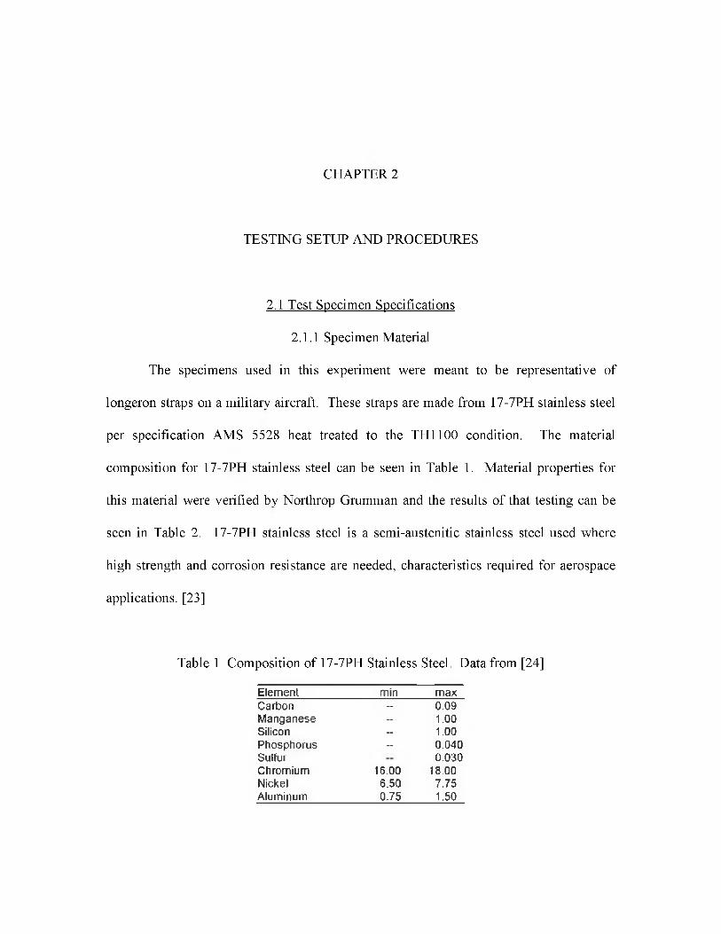
composition for 17-7PH stainless steel can be seen in Table 1. Material properties for
this material were verified by Northrop Grumman and the results of that testing can be
seen in Table 2. 17-7PH stainless steel is a semi-austenitic stainless steel used where
high strength and corrosion resistance are needed, characteristics required for aerospace
applications. [23]
Table 1 Composition of 17-7PH Stainless Steel. Data from [24]
Element min maxCarbon — 0.09Manganese — 1.00Silicon — 1.00Phosphorus — 0.040Sulfur 0.030Chromium 16.00 18.00Nickel 6.50 7.75Aluminum 0.75 1.50
17
Table 2 Material Properties of 17-7PH TH1100 Stainless Steel. Data from [25]
Properties Tensile Strength (ksi) Yield Strength (ksi) % ElongationAvg. 168.9 156.8 12.5
2.1.2 Test Specimen Fabrication
These particular test specimens were simplified for ease o f testing and to meet
several of the recommendations of ASTM E 647, a standard for testing methods to
determine fatigue crack growth rates. The test specimens, on average, measured 16
inches in length, 4 inches wide and 0.125 inches thick with a 0.157 inch center hole.
Located along the centerline o f the hole and 90 degrees to the load path was a notch that
served as a crack starter. GT270KB003 is the drawing for the test specimens and is
shown in Fig. 3. The certification sheets detailing the manufacturing and testing of the
specimen material can be seen in Appendix A. The specimens were provided by
Northrop Grumman.
The specimens were all manufactured from sheets of the same heat treatment lot
with the grains running in the longitudinal direction of the specimens. Making all the
specimens in this manner reduces variability in the testing. After the test specimens were
heat treated and fabricated, they were shot peened on both ends to reduce the risk o f
fatigue cracks growing near the fatigue machine grips. The final step in fabricating the
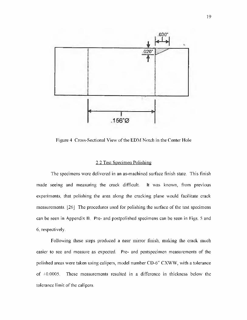
test specimens was to machine a notch in the bore perpendicular to the load path. This
was done using an electrical discharge machining (EDM) process. See Fig. 4 for a cross
sectional view of the machined notch. In total, 33 test specimens were delivered, 15 for
the test and 6 spares with the remaining 12 to be used for another program.
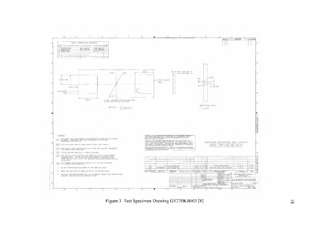
Figure 3 Test Specimen Drawing GT270KB003 [8] 18
19
030“
_ * H-H.020”
T
- 156”0
Figure 4 Cross-Sectional View of the EDM Notch in the Center Hole
2.2 Test Specimen Polishing
The specimens were delivered in an as-machined surface finish state. This finish
made seeing and measuring the crack difficult. It was known, from previous
experiments, that polishing the area along the cracking plane would facilitate crack
measurements. [26] The procedures used for polishing the surface of the test specimens
can be seen in Appendix B. Pre- and postpolished specimens can be seen in Figs. 5 and
6, respectively.
Following these steps produced a near mirror finish, making the crack much
easier to see and measure as expected. Pre- and postspecimen measurements of the
polished areas were taken using calipers, model number CD-6” CXWW, with a tolerance
of ±0.0005. These measurements resulted in a difference in thickness below the
tolerance limit o f the calipers.

20
« p
Figure 5 As-received Test Specimen
Figure 6 Polished Test Specimen
2.3 Test Equipment
During the fatigue testing for this study, the primary test system experienced a
malfunction. The result was that two different laboratories were used to conduct the
testing. One of the labs used to perform the testing is located at Hill AFB, UT in the
Science and Engineering Laboratory. The other lab used to conduct the testing is located
at SwRI in San Antonio, TX. The following sections give information about the
equipment used at Hill AFB lab to give the reader an idea of what was used during
testing. Details of the equipment used at SwRI can be seen in Appendix C. All tests
were conducted in lab air conditions.
2.3.1 Fatigue Machine and Equipment Specifications
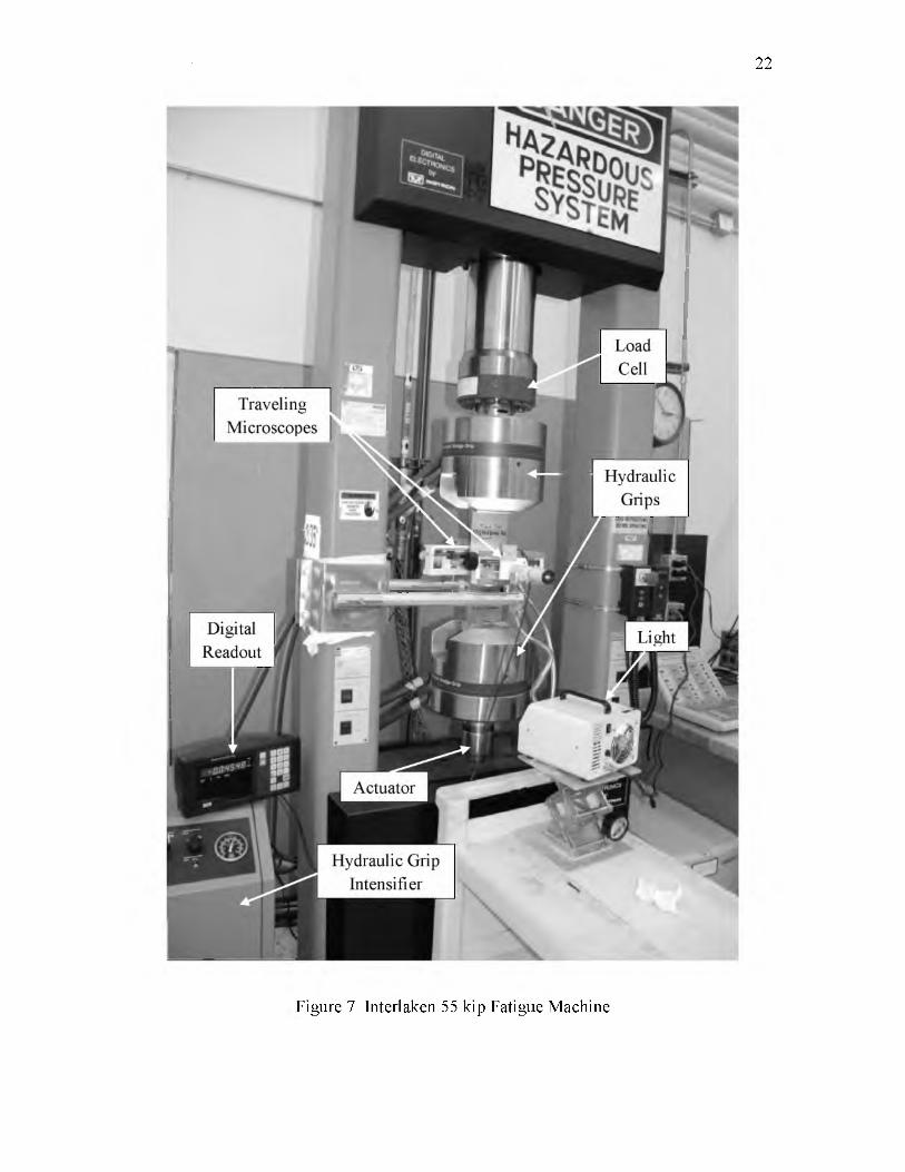
2.3.1.1 Interlaken Series 3300 55 kip Fatigue Machine
Interlaken was the original manufacturer o f the load frame used to conduct the
testing. The actuator on this machine has a 55 kip capacity and can be seen in Fig. 7.
The actuator is located below the specimen, has a ± 3 inch range and is equipped with a
positioning sensor. Above the specimen is the crosshead to which the Interface 50 kip
load cell, model 1032AF-50K-B, is attached. The load cell provides the feedback to the
controller indicating how much load is being applied to the specimen. Every year, the
fatigue machine and load cell must be calibrated to ensure the accuracy o f the
experiments performed. The calibration for these items was performed by Instron
Corporation on 4/15/13 for the fatigue machine and 4/16/13 for the load cell in
accordance with ASTM E4. The calibration certifications can be seen in Appendix D.
The testing done for this experiment was done within the year calibration timeframe. The
21
22
Figure 7 Interlaken 55 kip Fatigue Machine

alignment o f the grips, which is necessary to prevent unexpected loading, met
specification ASTM E1012 requirements.
2.3.1.2 MTS Hydraulic Wedge Grips
Hydraulic wedge grips, model 647, were used during this experiment in lieu o f
other gripping techniques. Using hydraulic grips simplifies the specimen installation
process and reduces variability with mechanical grips. This is due to the fact that
techniques require bolts to clamp onto the specimen, which require holes to be drilled
creating stress concentration areas. These specific grips have a 55 kip capacity with a
grip area that is 2.5 inches long by 4 inches wide. The MTS hydraulic wedge grips can
be seen in the middle o f Fig. 7.
2.3.1.3 MTS Hydraulic Over Hydraulic Intensifier
This particular model of hydraulic grips requires a hydraulic intensifier to
increase line pressure from 3,000 psi to a maximum of 10,000 psi depending on the
maximum load to be applied, static or fatigue. Based on this testing, the pressure was set
at 5,400 psi in order to maintain consistent gripping throughout the tests while not
providing too much clamp pressure, thus reducing the chance of a grip failure.
2.3.1.4 Instron 8800 Fast Track Controller and Software
An Instron 8800 series controller was used with different Instron software
packages. The Bluehill 2 software was used for tuning, balancing and constant amplitude
23
loading. Tuning and balancing o f the fatigue machine was necessary for every sample to
ensure the accuracy of the data being collected.
As part of the Bluehill 2 software package, the constant amplitude model, called
WaveMatrix, was used during the precracking phase of this experiment. This program
allows one to select the wave shape, frequency and amplitude at which the test will be
conducted. The only other piece of information needed to conduct the test is the mean
stress, which is the value established by the user in the setpoint window of the Bluehill 2
module. The details of how the precracking was performed will be explained later.
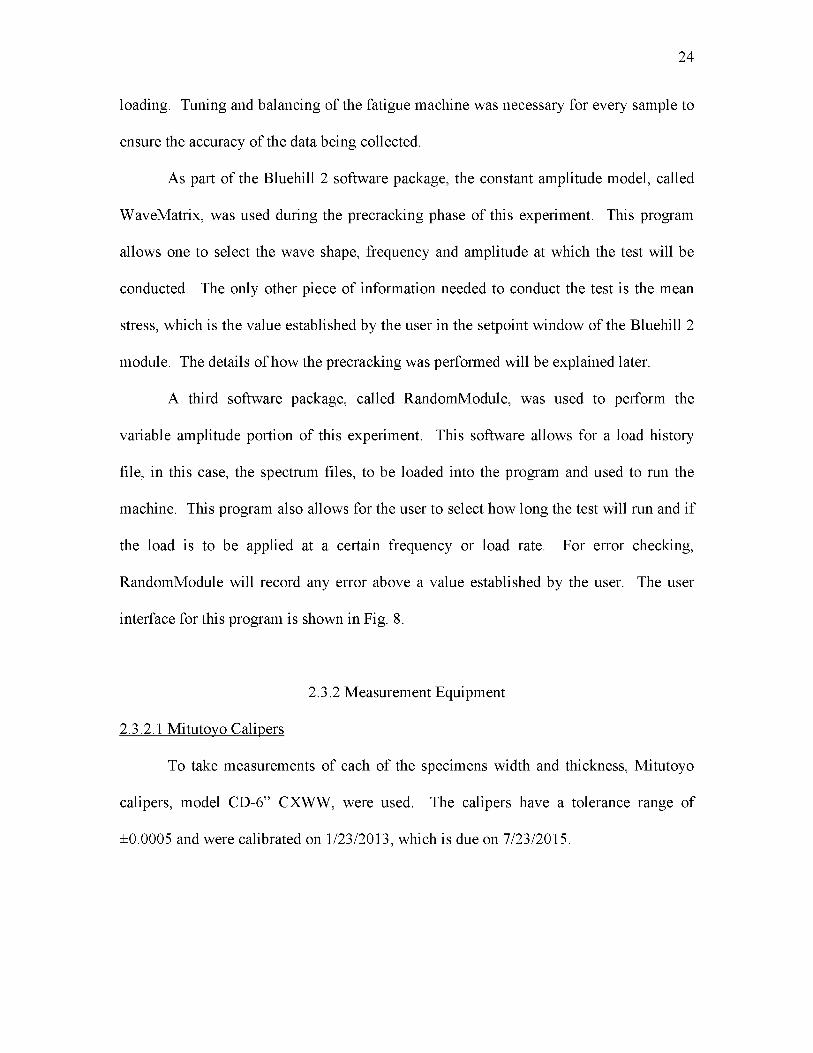
A third software package, called RandomModule, was used to perform the
variable amplitude portion o f this experiment. This software allows for a load history
file, in this case, the spectrum files, to be loaded into the program and used to run the
machine. This program also allows for the user to select how long the test will run and i f
the load is to be applied at a certain frequency or load rate. For error checking,
RandomModule will record any error above a value established by the user. The user
interface for this program is shown in Fig. 8.
2.3.2 Measurement Equipment
2.3.2.1 Mitutoyo Calipers
To take measurements o f each o f the specimens width and thickness, Mitutoyo
calipers, model CD-6” CXWW, were used. The calipers have a tolerance range o f
±0.0005 and were calibrated on 1/23/2013, which is due on 7/23/2015.
24
25
Figure 8 Random Module Interface
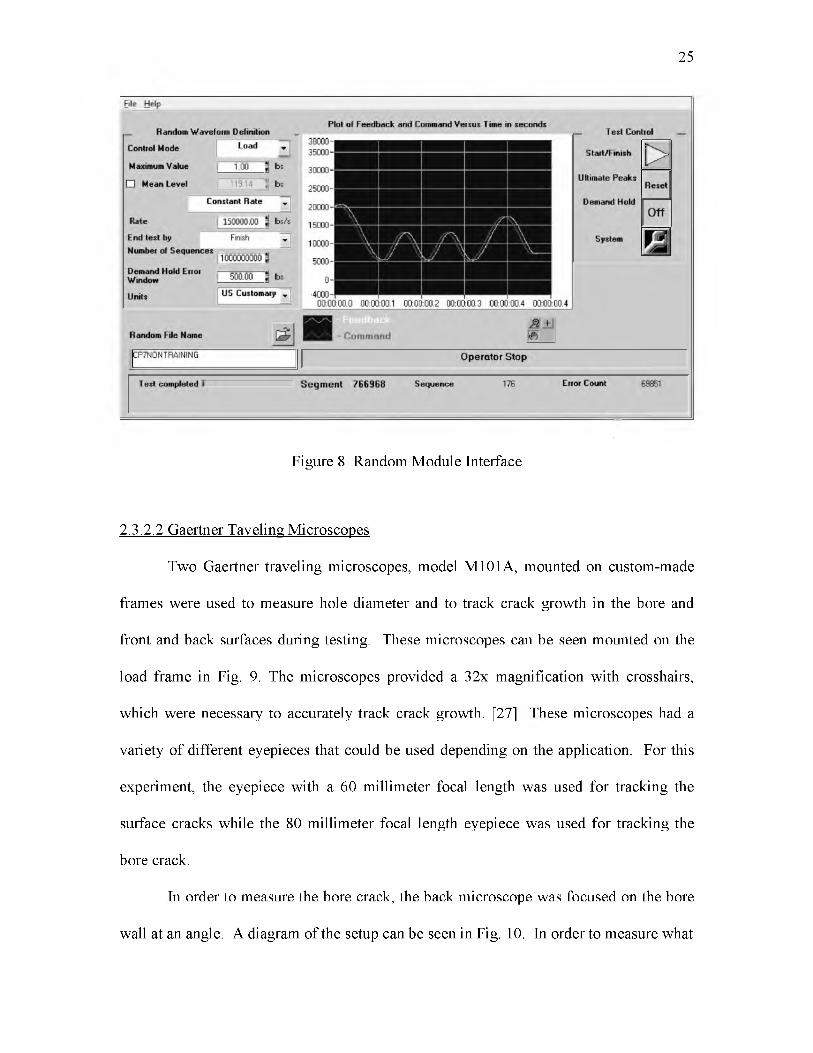
2.3.2.2 Gaertner Taveling Microscopes
Two Gaertner traveling microscopes, model M101A, mounted on custom-made
frames were used to measure hole diameter and to track crack growth in the bore and
front and back surfaces during testing. These microscopes can be seen mounted on the
load frame in Fig. 9. The microscopes provided a 32x magnification with crosshairs,
which were necessary to accurately track crack growth. [27] These microscopes had a
variety of different eyepieces that could be used depending on the application. For this
experiment, the eyepiece with a 60 millimeter focal length was used for tracking the
surface cracks while the 80 millimeter focal length eyepiece was used for tracking the
bore crack.
In order to measure the bore crack, the back microscope was focused on the bore
wall at an angle. A diagram of the setup can be seen in Fig. 10. In order to measure what
26
Figure 9 Gaertner Microscopes, Front and Back, Used to Take Measurements
the crack length was in the bore, the angle at which the traveling microscope was placed
needed to be known. Calculating the angle was accomplished by using simple
trigonometric concepts of right triangles. If the thickness of the specimen is known and
the apparent thickness of the specimen, through the microscope, can be measured, then
one can calculate the angle of the microscope using the following formula.

27
Microscope Direction of Motion
Microscope MicroscopePosition 1 Position 2
Hole
Unknown Angle 9
Figure 10 Illustration of Microscope Setup for Bore Measurements [26]
0 = sin - iV A ctual th ickness )
Once the angle of the microscope is determined, the crack length in the bore can be
calculated by simply rearranging the same formula. The only difference at this point is
that the measured crack length is now the variable for crack length as shown in the
following formula.
M easured crack leng thCrack L eng th =
sin(0)

The measurements from the microscopes were displayed on Fagor Automation
digital readouts. The tolerance range on the Fagor readouts is ±0.00002, which exceeds
the requirements of ±0.004 required by ASTM E647. One of the readouts can be seen
mounted on the hydraulic intensifier in Fig. 7.
2.3.2.3 AmScope Lamp
To increase the visibility of the crack, an AmScope lamp, model HL150-AY, was
used to illuminate the specimen. This lamp incorporates two snake lights, which could be
put in any position necessary to illuminate the crack. Images of the lamp can be seen in
Figs. 7 and 9.
2.4 Reaming and Bore Polishing
2.4.1 Reaming
After the precracking was performed on each of the specimens, the center hole
was reamed from a 0.157” hole to a 0.250” hole, which is representative of a fastener
hole. The procedure used for reaming the bore can be seen in Appendix B. The reaming
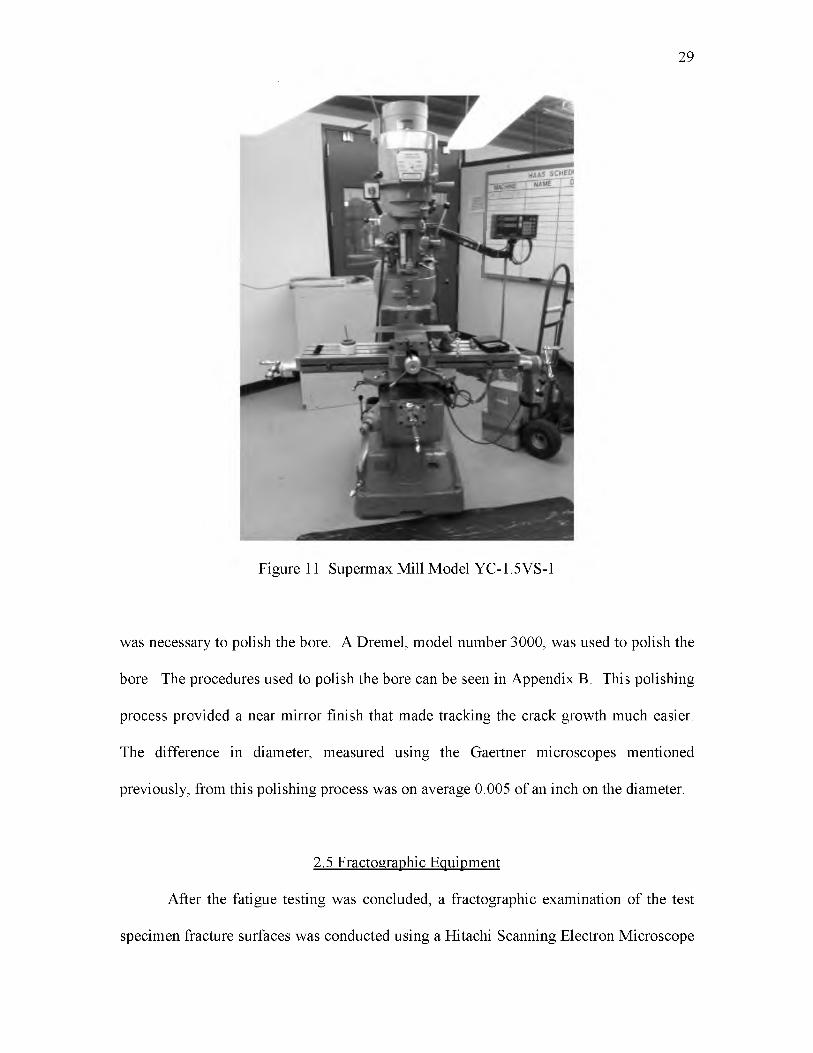
operation was performed on a Supermax Mill, model YC-1.5VS-1 and seen in Fig. 11, is
manufactured by the Jih Fong Machinery Co. LTD. The dial indicator used to find the
center of the bore is accurate to within 0.001 of an inch.
2.4.2 Bore Polishing
After the reaming was performed, the bore surface had machining marks, which
made it difficult to view the crack. To obtain better visibility of the crack in the bore, it
28
29
Figure 11 Supermax Mill Model YC-1.5VS-1
was necessary to polish the bore. A Dremel, model number 3000, was used to polish the
bore. The procedures used to polish the bore can be seen in Appendix B. This polishing
process provided a near mirror finish that made tracking the crack growth much easier.
The difference in diameter, measured using the Gaertner microscopes mentioned
previously, from this polishing process was on average 0.005 of an inch on the diameter.
2.5 Fractographic Equipment
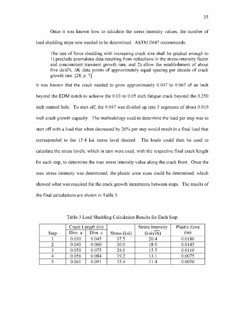
After the fatigue testing was concluded, a fractographic examination of the test
specimen fracture surfaces was conducted using a Hitachi Scanning Electron Microscope
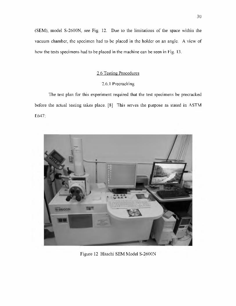
(SEM), model S-2600N, see Fig. 12. Due to the limitations of the space within the
vacuum chamber, the specimen had to be placed in the holder on an angle. A view of
how the tests specimens had to be placed in the machine can be seen in Fig. 13.
2.6 Testing Procedures
2.6.1 Precracking
The test plan for this experiment required that the test specimens be precracked
before the actual testing takes place. [8] This serves the purpose as stated in ASTM
E647:
30
Figure 12 Hitachi SEM Model S-2600N

31
Figure 13 Position of Fatigue Specimen Once Inside the SEM
to provide a sharpened fatigue crack of adequate size and straightness which ensures that 1) the effect of the machined starter notch is removed from the specimen K-calibration, and 2) the effects on subsequent crack growth rate data caused by changing crack front shape or pre-crack load history are eliminated. [28, p. 6]
As mentioned previously, each specimen started off with a 0.157” hole with a 0.020” by
0.030” triangular-shaped EDM corner notch placed perpendicular to the load path. The
EDM notch serves as a stress concentrator to get the crack started.
The test plan also specified that a constant amplitude cyclic load be applied to the
specimens that would result in precracks 0.030 to 0.050 of an inch in length beyond the
final ream sized hole. [8] These precracks were representative of flaws in the material
that are assumed to be present according to the Damage Tolerant philosophy. [6] The
size of the precrack was chosen because 0.030” to 0.050” is the NDI detectable limit. [6]
The Constant amplitude loading was applied at 15.4 ksi and a stress ratio of 0.05. [8] The
15.4 ksi stress, which is 70% of the max stress in the test, was chosen because ASTM
E647 requires that any precracking performed end with a max stress intensity that is
lower than the initial stress intensity o f the test. [28] A complication that arises from this
ASTM E647 requirement is that it was intended for constant amplitude loading and
mentions nothing for variable amplitude loading, which is what was used during actual
testing. It was determined that as long as the final precracking stress intensity was less
than the initial max stress intensity created by the highest load in the spectrum, the intent
of E647 requirement would be met.
2.6.1.1 Load Shedding
Soon after the precracking on the first sample was initiated, it became apparent
that something needed to be done to speed up the process. Initially, the precracking ran
for several hours at the 15.4 ksi stress level with no detectable crack progression. ASTM
E647 specifies a load shedding technique that can be used to speed up the precracking
process. Load shedding is a process where one runs the sample at a high load to get the
crack started from the notch. The load is then progressively decreased over a number o f
steps until the final step is at the desired stress level. A graph that illustrates the load
shedding concept is shown in Fig. 14.
One of the load shedding requirements from ASTM E647 is that each step must
be run long enough to get through the plastic zone of the previous load shedding step.
[28] Another requirement is that there can be no more than a 20% drop difference
32

33
Figure 14 Plot Demonstrating the Load Shedding Concept [28]
between the final load max of one step and the beginning load max of the next step. The
requirements are to reduce, as much as possible, any transient effects that occur from the
plastic zones from one step to the next. [28] To determine the crack size increments for
each step, E647 suggested using the following formula, which is the formula for
calculating plastic zone sizes. [28]
A a= ©3 \ (K'r
°YS
2

34
Here, Aa is the crack size increment, K'max is the terminal value of Kmax from the
previous step. The difficulty that arises from using this formula is determining the
experiment, particularly the EDM notches, differs from that typically used in the E647
test. The middle tension specimens in E647 have a hole in the center, just like this
experiment, but with two, through thickness notches on opposite sides of the hole
perpendicular to the load path. The specimens used in this experiment had only one
corner notch, which requires a different formula to determine the K'max value.
The formulas used to determine the K'max value were obtained from the
Handbook of Stress Intensity Factors. [29] The primary function is the following
equation, which was derived from finite element results. [29] A step-by-step process of
how this function is used is shown in Appendix E. [29]
K is the stress intensity at a point along the curve at angle 0 , which is in radians. [29] St
is the tension stress, a is the crack length in the bore, c is the crack length on the surface,
t is the specimen thickness, b is the width of the specimen and r is the hole radius. [29]
Q is expressed in the following equation. [29]
where a and c are the same as the previous function. It was assumed that the aspect ratio,
a /c , remained a constant 0.667.
correct K'max value. This is due to the fact that geometry of the specimens used in themax
35
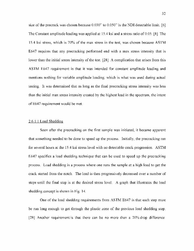
Once it was known how to calculate the stress intensity values, the number o f
load shedding steps now needed to be determined. ASTM E647 recommends:
The rate of force shedding with increasing crack size shall be gradual enough to 1) preclude anomalous data resulting from reductions in the stress-intensity factor and concomitant transient growth rate, and 2) allow the establishment o f about five da/dN, AK data points of approximately equal spacing per decade of crack growth rate. [28, p. 7]
It was known that the crack needed to grow approximately 0.047 to 0.067 of an inch
beyond the EDM notch to achieve the 0.03 to 0.05 inch fatigue crack beyond the 0.250
inch reamed hole. To start off, the 0.047 was divided up into 5 segments of about 0.010
inch crack growth capacity. The methodology used to determine the load per step was to
start o ff with a load that when decreased by 20% per step would result in a final load that
corresponded to the 15.4 ksi stress level desired. The loads could then be used to
calculate the stress levels, which in turn were used, with the respective final crack length
for each step, to determine the max stress intensity value along the crack front. Once the
max stress intensity was determined, the plastic zone sizes could be determined, which
showed what was required for the crack growth increments between steps. The results of
the final calculations are shown in Table 3.
Table 3 Load Shedding Calculation Results for Each Step
StepCrack Length (in)
Stress (ksi)Stress Intensity
(ksiVm)Plastic Zone
(in)Dim. a Dim. c1 0.030 0.045 37.5 20.4 0.01802 0.040 0.060 30.0 18.0 0.01453 0.050 0.075 24.0 15.5 0.01104 0.056 0.084 19.2 13.1 0.00755 0.061 0.091 15.4 11.4 0.0050

2.6.2 Fatigue Testing
To compare the two spectra developed for this research, five different
combinations of the spectra were tested. These different combinations were given the
following nomenclature: A baseline, A plus B_1, A plus B_2, A plus B_3 and B baseline
tests. For each combination, three specimens were used to establish a level of confidence
in the results. The baseline tests, A and B showed how each spectrum performed
individually. The mixed spectra tests were set up to run the A spectrum first then
transition to the B spectrum when the bore crack length reached a predetermined range.
The differences between the mixed spectra tests were that the transitions from A to B
occurred at different crack lengths. This was done because no two aircraft have
experienced the exact same usage; hence, a range of crack size applicability had to be
considered in the testing. Thus, the B_1 to B_3 tests were meant to show a progression
of effective flight hours (EFH) spent under A loading condition. B_1 tests represent the
least amount of time an aircraft spent under A loading conditions while B_3 tests
represented the most. The attributes for each spectrum are shown in Table 4.
Before actual testing began, the test run order was randomized. This was done to
reduce any abnormalities that may occur while testing from skewing the test data. For
instance if all of the A baseline tests were done sequentially while some error had
occurred in the machine, then all of the data for those specimens would be affected. But
36
Table 4 Test Spectra Attributes. Data from [8]
SpectrumGmax(psi)
axma)
o(
L Gmin(psi)
Loadmin(lb)
Blocksize(Hours)
Endpoints per Block
A 21,953 10,977 197 99 240 16,731B 21,953 10,977 266 133 1,000 4,371
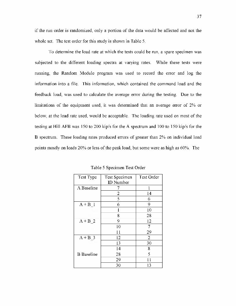
if the run order is randomized, only a portion of the data would be affected and not the
whole set. The test order for this study is shown in Table 5.
To determine the load rate at which the tests could be run, a spare specimen was
subjected to the different loading spectra at varying rates. While these tests were
running, the Random Module program was used to record the error and log the
information into a file. This information, which contained the command load and the
feedback load, was used to calculate the average error during the testing. Due to the
limitations of the equipment used, it was determined that an average error of 2% or
below, at the load rate used, would be acceptable. The loading rate used on most of the
testing at Hill AFB was 150 to 200 kip/s for the A spectrum and 100 to 150 kip/s for the
B spectrum. These loading rates produced errors of greater than 2% on individual load
points mostly on loads 20% or less of the peak load, but some were as high as 60%. The
37
Table 5 Specimen Test Order
Test Type Test Specimen ID Number
Test Order
A Baseline 7 12 145 6
A + B 1 6 91 108 28
A + B 2 9 1210 711 29
A + B 3 12 213 3014 8
B Baseline 28 529 1130 13

max load variation producing the error was 135 lb. The equipment used at Hill AFB
made managing the error any better than what was observed difficult. SwRI was able to
keep all points below 2% error while running at 100 kip/s. Therefore, it is recommended
that the load rate be reduced to better manage the error.
2.7 AFGROW Procedures
As has been stated, AFGROW is a program used to model crack growth behavior
subject to fatigue. Essentially, how this program works is it uses the inputs provided by
the user, i.e., geometry of the sample, material used, loading conditions etc., and
calculates how much the crack will grow on each load cycle. [30] Starting with an initial
flaw size, the program calculates the stress intensity on the crack front and uses that
information to determine how much the crack will grow on that cycle. This process is
repeated cycle per cycle until certain failure or termination criteria are met. The analysis
for this study was conducted using procedures, seen in Appendix F, which were based on
a set of guidelines prepared by the USAF. [31] Fig. 15 is an image of the AFGROW
interface.
As was mentioned earlier, past research showed that Yield Zone and Crack
Closure crack growth retardation models provided good fits to steel type materials tested
under similar conditions. However, soon after starting the modeling process, it was
discovered that better fits to the data could be obtained when no retardation models were
utilized. Further discussion on this topic can be seen in section 4.3.
38
39
Figure 15 AFGROW Interface
2.8 Data Collection and Test Matrix
Excel spreadsheets were used to collect the data during fatigue testing. These
data sheets identified the specimen and what type of test was performed. Concerning the
specimens themselves, the following measurements were recorded: specimen thickness,
specimen width, EDM notch length, pre- and postream center bore diameter and
postream corner crack surface and bore lengths. Other items of interest that were
recorded on the data sheets were testing dates, load conditions, load rates and comments.
An example of a crack growth data sheet can be seen in Fig. 16.
Concerning the frequency on which measurements should be recorded during the
test, the researchers took into consideration a guideline in ASTM E647. This
specification recommends that measurements be recorded on a minimum of 0.004 of an
inch crack growth. [28] Having said that, the same specification also states that the,
0.004 of an inch, measurement could be adjusted depending on the circumstances. [28]

40
GT270KB003-13-5 Fatigue Crack Growth Data SheetWidth: 4.004 in. Thick: 0.125 in. Area: 0.501 in
Pre-crack InformationPre-crack Date: 6/4/13 Hole Dia.: 0.157 in.
Loading Condition: Constant Amplitude R=0.05 Surface EDM: 0.0298 in.
Pre-crack Tuning DataTuning Step Frequency (Hz) Tuning Cycles Max Stress (ksi)
1 13 1977 37.52 15 1923 243 18 2940 15.4
Pre-crack Run DataCycles Stress (ksi) Frequency (Hz) Crack Length (in.)
0 0 0 0.108332759 37.5 13 0.123354099 30 13 0.139792092 24 15 0.1529128284 19.2 15 0.1620173327 15.4 18 0.1687
Experiment InformationExp. Date: 2/11/14 Loading Condition: Variable AmplitudeExp. Type: Spec. A Loading Rate: 400 to 500 kip/s Hole Dia.: 0.253 in.Max Stress (Sp. A): 21.953 ksi Surface Crack: 0.046 in. Bore Crack: 0.082 in.
Experiment Run Data
Spectrum EFHCrac c Length (in.)
CommentsFront Bore BackA 0 0.046 0.082 500 kip/s
4497.77 0.048 0.08225347.35 0.069 0.09845425.05 0.090 0.116 Reduced to
400 kip/s due to limit
trip
66581.12 0.120 0.125 0.07384059.44 0.153 0.109107210.63 0.193 0.163129839.13 0.244 0.221152402.17 0.305 0.284
Figure 16 Example of a Crack Growth Data Sheet

Thus, it was anticipated that measurements would be recorded in these small increments
during the initial stages of the test, then increase to larger increments as the tests
proceeded. The test matrix used for this research is shown in Table 6.
Table 6 Fatigue Testing Matrix
41
No. of Specimens
Tested IdentificationSpectrum and
Sequence Test Sequence
3 Baseline A A onlyBaseline, testing from initial crack to at least 100,000 EFH with this
spectrum
3 A + B_1 A + BSpectrum A testing until initial
crack grows to a = 0.090 to 0.095”, then switch to spectrum B
3 A + B_2 A + BSpectrum A testing until initial
crack grows to a = 0.105 to 0.110”, then switch to spectrum B
3 A + B_3 A + BSpectrum A testing until initial crack grows through thickness,
then switch to spectrum B
3 Baseline B B onlyBaseline, testing from initial crack to at least 100,000 EFH with this
spectrum

CHAPTER 3
RESULTS
3.1 Accelerated Fatigue Tests
The results shown in this chapter are based on data gathered from testing
conducted at both Hill AFB and SwRI. It is important to note that both Hill AFB and
SwRI conducted at least one of each type of test. It was not originally planned to perform
fatigue tests at two locations, but it helped to determine if any error occurred due to the
equipment being used. Each of the five variations of tests used three test specimens. The
data sheets for all of the fatigue testing conducted can be seen in Appendix G.
Additionally, curves not displayed in the section can be seen in Appendix H
3.1.1 Spectrum A Baseline
Baseline data for spectrum A were developed for comparison purposes with
spectrum B and analytical data. Whenever possible, it is a good idea to validate
analytical data with testing results. Specimens designated as GT270-2, -5 and -7 were
used to conduct these tests. The average bore and front surface cracks for these
specimens were 0.074 and 0.044 of an inch, respectively. Fig. 17 plots the crack lengths
vs. EFH of the fatigue testing conducted to establish the baseline for spectrum A. The
plot shows that all three tests agree very well until about 200,000 EFH, at which point
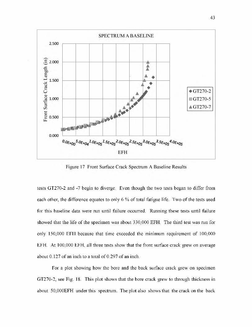
43
tests GT270-2 and -7 begin to diverge. Even though the two tests began to differ from
each other, the difference equates to only 6 % of total fatigue life. Two of the tests used
for this baseline data were run until failure occurred. Running these tests until failure
showed that the life of the specimen was about 330,000 EFH. The third test was run for
only 150,000 EFH because that time exceeded the minimum requirement of 100,000
EFH. At 100,000 EFH, all three tests show that the front surface crack grew on average
about 0.127 of an inch to a total of 0.297 of an inch.
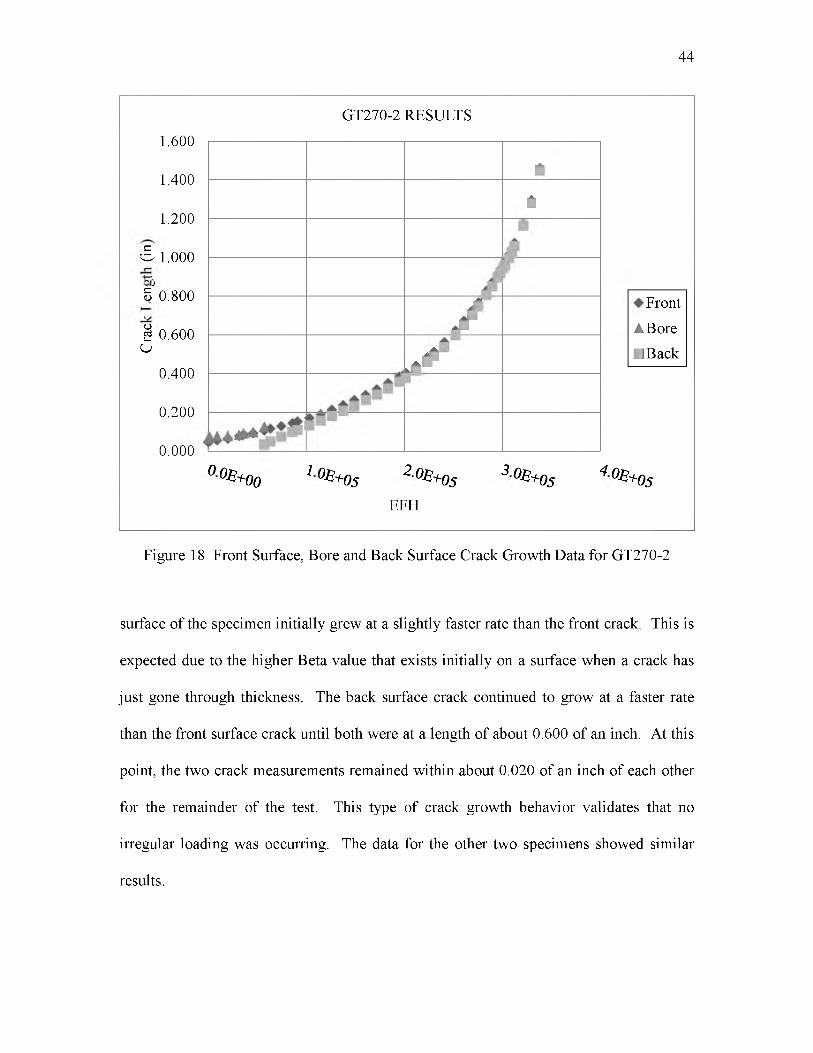
For a plot showing how the bore and the back surface crack grew on specimen
GT270-2, see Fig. 18. This plot shows that the bore crack grew to through thickness in
about 50,000EFH under this spectrum. The plot also shows that the crack on the back
44
GT270-2 RESULTS
1.600
1.400
1.200
£ 1.000 h htg
8 0.800 L
§ 0.600 o
0.400
0.200
0.000
i
i
/s
Front
A Bore
■ Back
° ° E + 0 0 l 0E+05 2 °E + 0 s 3 °E +05 4 °E + 0s
EFH
Figure 18 Front Surface, Bore and Back Surface Crack Growth Data for GT270-2
surface of the specimen initially grew at a slightly faster rate than the front crack. This is
expected due to the higher Beta value that exists initially on a surface when a crack has
just gone through thickness. The back surface crack continued to grow at a faster rate
than the front surface crack until both were at a length of about 0.600 of an inch. At this
point, the two crack measurements remained within about 0.020 of an inch of each other
for the remainder of the test. This type of crack growth behavior validates that no
irregular loading was occurring. The data for the other two specimens showed similar
results.
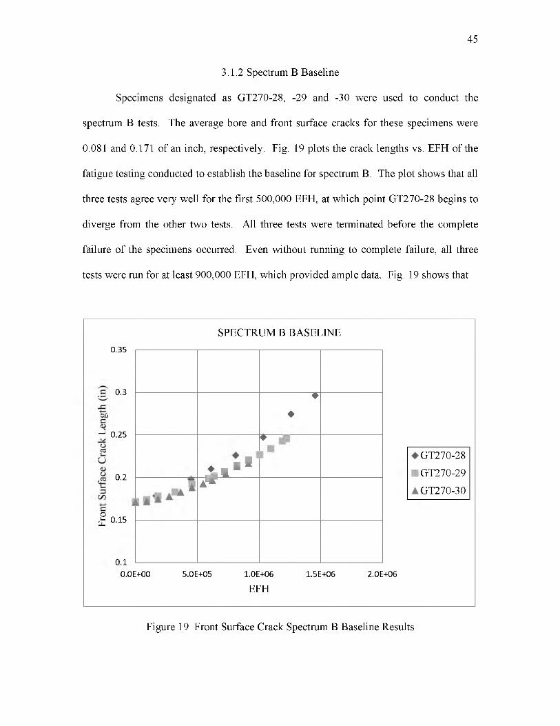
3.1.2 Spectrum B Baseline
Specimens designated as GT270-28, -29 and -30 were used to conduct the
spectrum B tests. The average bore and front surface cracks for these specimens were
0.081 and 0.171 of an inch, respectively. Fig. 19 plots the crack lengths vs. EFH of the
fatigue testing conducted to establish the baseline for spectrum B. The plot shows that all
three tests agree very well for the first 500,000 EFH, at which point GT270-28 begins to
diverge from the other two tests. All three tests were terminated before the complete
failure of the specimens occurred. Even without running to complete failure, all three
tests were run for at least 900,000 EFH, which provided ample data. Fig. 19 shows that
45
0.35
0.3htgne
^ 0.25kcarCeeac 0.2fr
>! °-15
n 1
SPECTRUM B BASELINE
♦
♦
♦ i - B
♦GT270-28
GT270-29
GT270-30A *
0.0E+00 5.0E+05 1.0E+06 1.5E+06 2.0E+06EFH
Figure 19 Front Surface Crack Spectrum B Baseline Results
even when the testing had ran for 450,000 EFH, the front surface crack had only grown
on average 0.021 of an inch to a total of 0.192 of an inch.
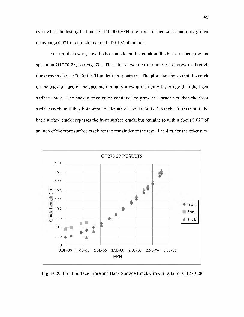
For a plot showing how the bore crack and the crack on the back surface grew on
specimen GT270-28, see Fig. 20. This plot shows that the bore crack grew to through
thickness in about 500,000 EFH under this spectrum. The plot also shows that the crack
on the back surface of the specimen initially grew at a slightly faster rate than the front
surface crack. The back surface crack continued to grow at a faster rate than the front
surface crack until they both grew to a length of about 0.300 of an inch. At this point, the
back surface crack surpasses the front surface crack, but remains to within about 0.020 of
an inch of the front surface crack for the remainder of the test. The data for the other two
46
GT270-28 RESULTS0.45
0.4
0.35
S 0.3
0.25n eL 0.2k
s °.15
0.1
0.05
00.0E+00 5.0E+05 1.0E+06 1.5E+06 2.0E+06 2.5E+06 3.0E+06
EFH
A
ii►
$♦
*A
4▼
■ ■A .
X1
II ■♦▲
♦ A♦ ▼ A
Front
Bore
A Back
Figure 20 Front Surface, Bore and Back Surface Crack Growth Data for GT270-28
specimens showed similar results except that the back surface cracks never exceed the
length measurements of the front surface cracks. The other difference on this specimen
was that the bore to back surface crack transition took place at about 614,000 EFH while
the others took on average about 686,000 EFH to make the same transition.
3.1.3 Combinations of Spectra A and B
Combination tests using both spectra were developed to directly determine how
17-7PH would behave during the transition from spectrum A to B. As was stated earlier,
the bore cracks were allowed to grow to three different ranges of length under spectrum
A before transitioning to spectrum B. This was done to represent the range in life of the
actual fleet of aircraft under spectrum A before the transition occurred to spectrum B. It
also allows investigators to determine if the crack growth behavior changes significantly
between the different transition points. Note that since these tests were conducted for
varying amounts of EFH, some of the plots were created with shortened data sets for
visualization purposes.
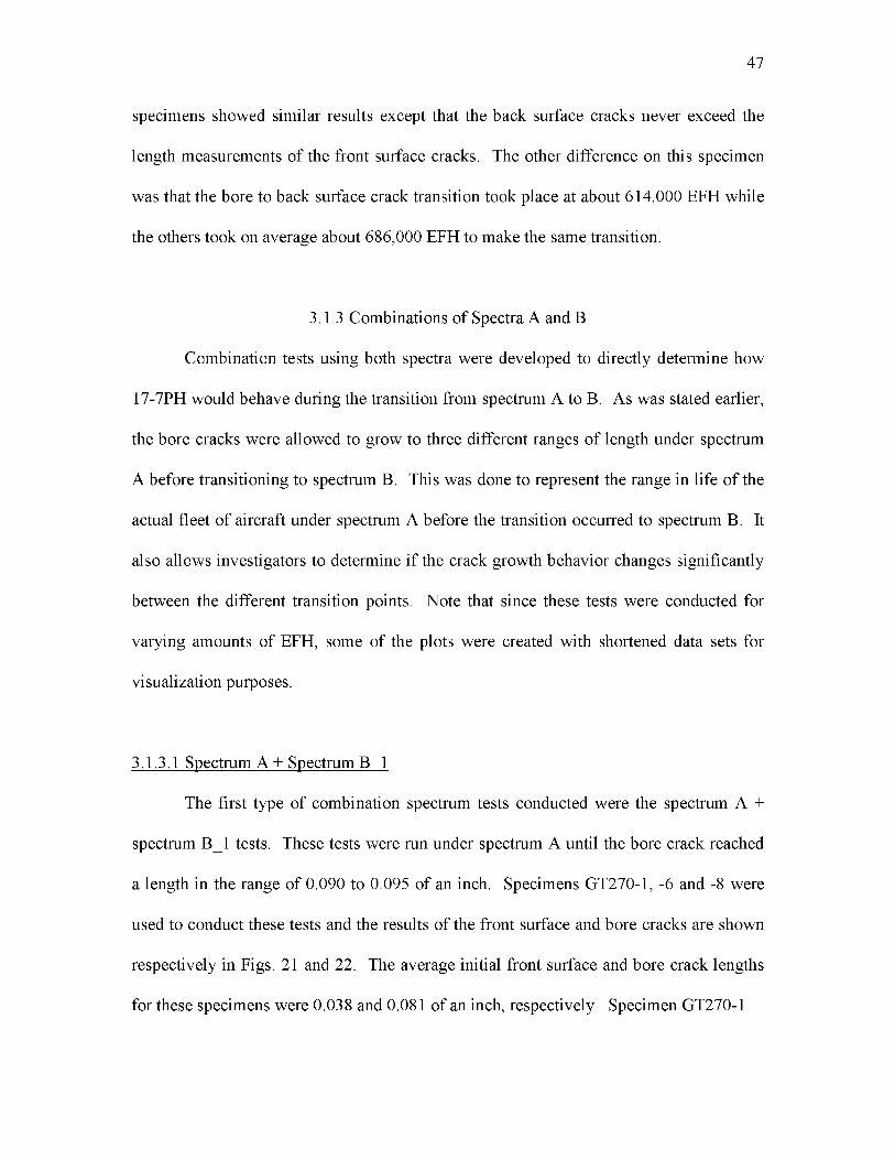
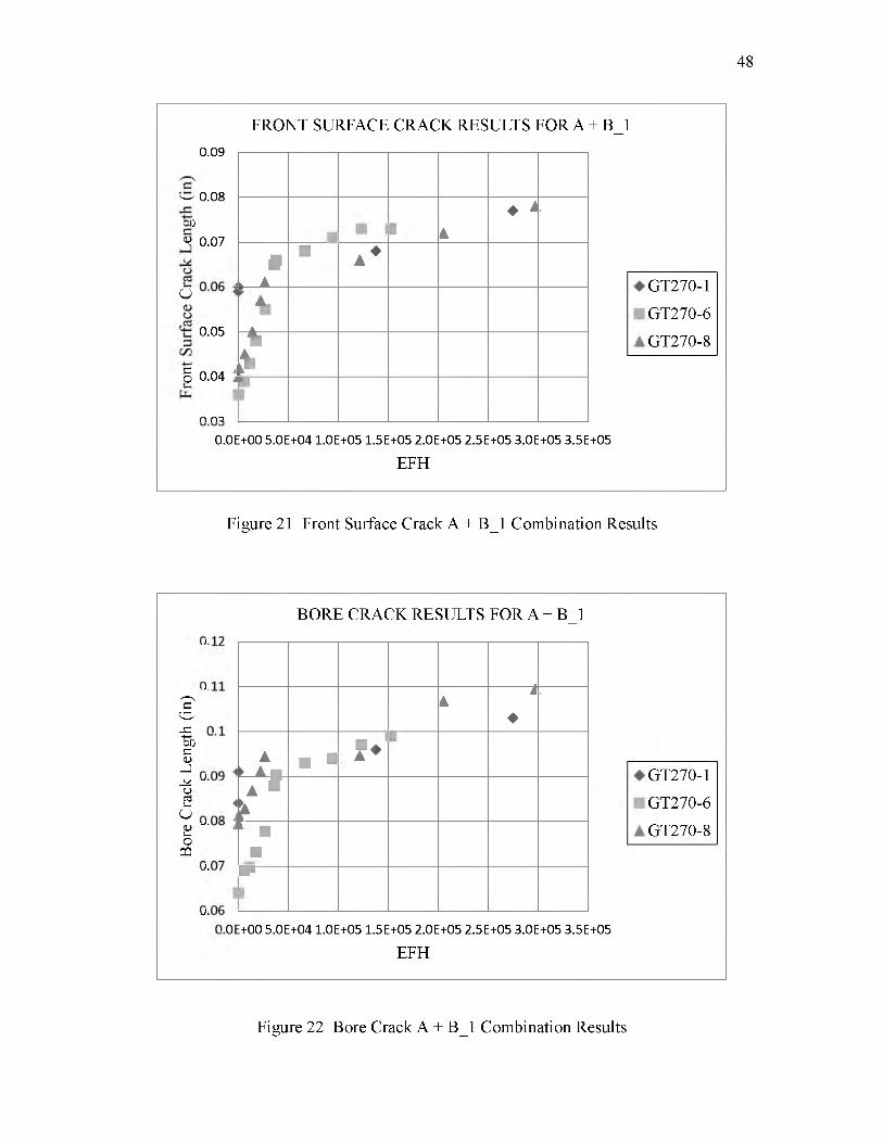
3.1.3.1 Spectrum A + Spectrum B 1
The first type of combination spectrum tests conducted were the spectrum A +
spectrum B_1 tests. These tests were run under spectrum A until the bore crack reached
a length in the range of 0.090 to 0.095 of an inch. Specimens GT270-1, -6 and -8 were
used to conduct these tests and the results of the front surface and bore cracks are shown
respectively in Figs. 21 and 22. The average initial front surface and bore crack lengths
for these specimens were 0.038 and 0.081 of an inch, respectively. Specimen GT270-1
47
48
0.09n)
W 0.08 h htng
v 0.07kcar
FRONT SURFACE CRACK RESULTS FOR A + B_1
1 4♦ ^ i
i t A
m A *GT270-1
GT270-6
GT270-8
oeca
0.05uSt
§ 0.04 rFn nQ
At i
t
0.0E+00 5.0E+04 1.0E+05 1.5E+05 2.0E+05 2.5E+05 3.0E+05 3.5E+05EFH
Figure 21 Front Surface Crack A + B_1 Combination Results
Bore
Crac
k Le
ngth
(in
)0.
0. 0.
0. 0
0. 0.
00
0 0
0 .
1 1
. O
BORE CRACK RESULTS FOR A + B_1
4A
♦
L
A ► A ■ ■ V
1
GT270-1
GT270-6
GT270-8
A 1jk
■■
W
+00 5.0E+04 1.0E+05 1.5E+05 2.0E+05 2.5E+05 3.0E+05 3.5E+05EFH
Figure 22 Bore Crack A + B_1 Combination Results
actually had larger initial crack sizes due to reasons that will be explained in section
4.1.2.1. The plots are the crack lengths vs. EFH of the fatigue testing conducted for the
spectrum A to spectrum B_1 transition. These plots show that all three tests agreed very
well as far as crack growth is concerned, with the exception of the initial measurements
of GT270-1. All three tests were terminated prior to specimen failure but only after the
minimum 100,000 EFH requirement had been met. For specimens GT270-6 and -8, the
transition to spectrum B occurred at about 37,000 and 26,000 EFH, respectively. Once
the transition to spectrum B was made, the crack growth essentially stalled for the
remainder of the test. All three tests showed that during the spectrum B portion, the
crack grew only 0.006 of an inch on average for 100,000 EFH.
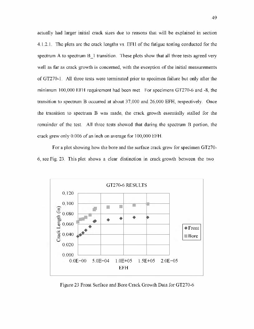
For a plot showing how the bore and the surface crack grew for specimen GT270-
6, see Fig. 23. This plot shows a clear distinction in crack growth between the two
49
0.120
) 0.100 n)i
^ 0.080 h tg
8 0.060 LH 0.040 r
C 0.020
n nnn
GT270-6 RESULTS
m ■ ■■
. ♦ ♦ ♦ ►
Front
Bore
0.0E+00 5.0E+04 1.0E+05 1.5E+05 2.0E+05EFH
Figure 23 Front Surface and Bore Crack Growth Data for GT270-6
different spectra. One can see from the plot of either crack that they grew under
spectrum A for about 0.025 of an inch in the 37,000 EFH period before transitioning to
spectrum B. After the transition to spectrum B was made, the front surface and bore
cracks grew approximately 0.007 and 0.009 of an inch, respectively, for 100,000 EFH.
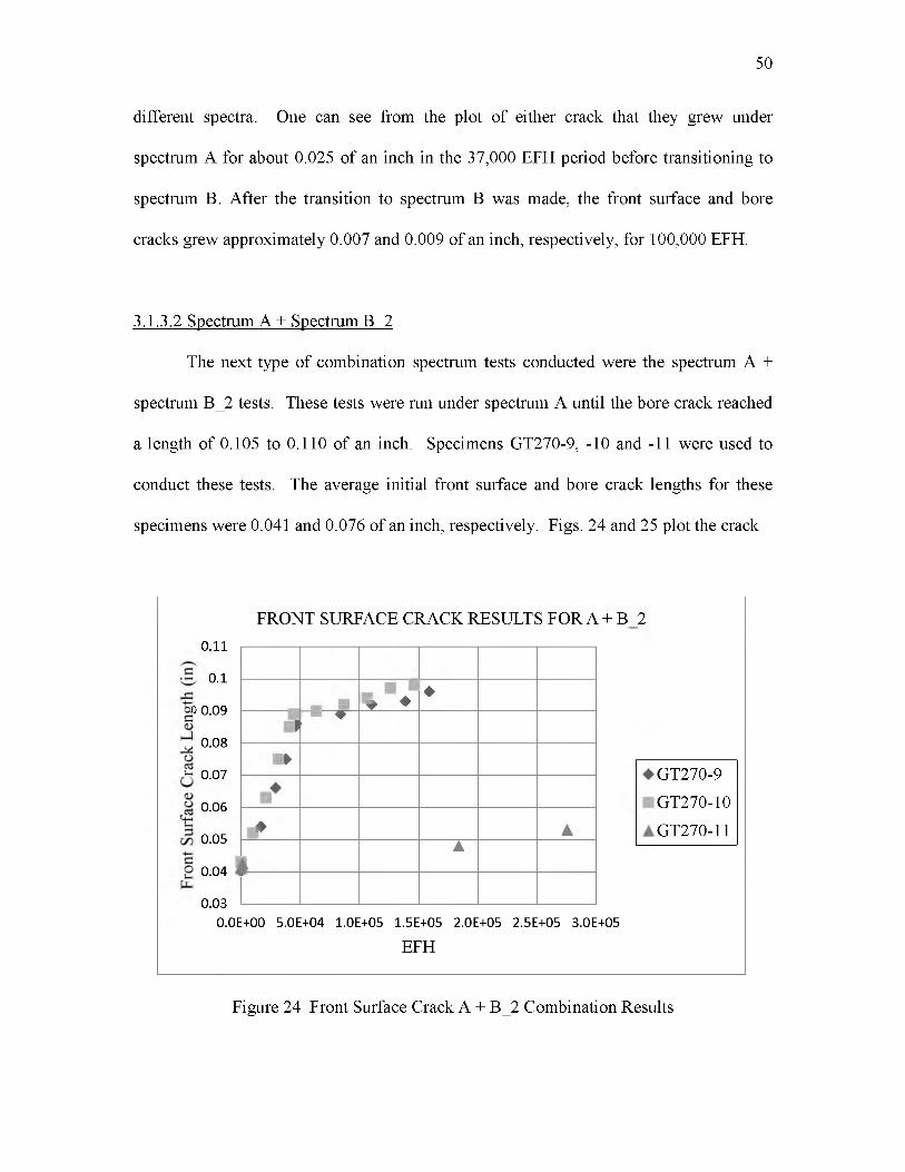
3.1.3.2 Spectrum A + Spectrum B 2
The next type of combination spectrum tests conducted were the spectrum A +
spectrum B_2 tests. These tests were run under spectrum A until the bore crack reached
a length of 0.105 to 0.110 of an inch. Specimens GT270-9, -10 and -11 were used to
conduct these tests. The average initial front surface and bore crack lengths for these
specimens were 0.041 and 0.076 of an inch, respectively. Figs. 24 and 25 plot the crack
50
FRONT SURFACE CRACK RESULTS FOR A + B 2
htgneeLkcarCecafruStnorF
0.11
0.1
0.09
0.08
0.07
0.06
0.05
0.04
0.03
* ♦♦
» ♦
►
♦ ▲▲
GT270-9
GT270-10
GT270-11
0.0E+00 5.0E+04 1.0E+05 1.5E+05 2.0E+05 2.5E+05 3.0E+05EFH
Figure 24 Front Surface Crack A + B_2 Combination Results

51
0.13
0.12n)i( 0.11
£ g en 0.1 eL kca0.09r
' i £ 0.08oB0 07 a
BORE CRACK RESULTS FOR A + B_2
♦■
■
<
♦ A A
1 ♦L GT270-9
GT270-10
GT270-11L 4 i m
*
0.060.0E
►
+00 5.0E+04 1.0E+05 1.5E+05 2.0E+05 2.5E+05 3.0E+05 EFH
Figure 25 Bore Crack A + B_2 Combination Results
lengths vs. EFH of the fatigue testing conducted for the spectrum A to spectrum B_2
transition. These plots show that the results agree well with each other except for the
results from specimen GT270-11. See section 4.1.2.1 for more details on specimen
GT270-11. All three tests were terminated prior to specimen failure after meeting the
minimum EFH requirement. For specimens GT270-9 and -10, the transition to spectrum
B occurred at about 47,000 and 44,000 EFH, respectively. As was seen in the spectrum
A + spectrum B_1 tests, the transition to spectrum B also caused the crack growth to
stall. All three tests showed that during the spectrum B portion of the test the crack grew
only 0.008 of an inch on average for 100,000 EFH.
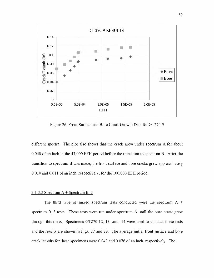
A plot showing how the bore and the surface crack grew for specimen GT270-9
see Fig. 26. This plot also shows the clear distinction in crack growth between the two
52
0.14
0.12
:? 0.1
^ 0.08 n
3 1 ~ °.°6kcar
GT270-9 RESULTS
■ ■■ ■ ■
■. ■ ♦ ♦
♦♦ ♦
♦♦
I
Front
Bore♦
0.02
00.0E+00 5.0E+04 1.0E+05 1.5E+05 2.0E+05
EFH
Figure 26 Front Surface and Bore Crack Growth Data for GT270-9
different spectra. The plot also shows that the crack grew under spectrum A for about
0.040 of an inch in the 47,000 EFH period before the transition to spectrum B. After the
transition to spectrum B was made, the front surface and bore cracks grew approximately
0.010 and 0.011 of an inch, respectively, for the 100,000 EFH period.
3.1.3.3 Spectrum A + Spectrum B 3
The third type of mixed spectrum tests conducted were the spectrum A +
spectrum B_3 tests. These tests were run under spectrum A until the bore crack grew
through thickness. Specimens GT270-12, 13- and -14 were used to conduct these tests
and the results are shown in Figs. 27 and 28. The average initial front surface and bore
crack lengths for these specimens were 0.043 and 0.076 of an inch, respectively. The

53
FRONT SURFACE CRACK RESULTS FOR A + B 3
htgneeLkcarCecafruStnorF
0.11
0.1
0.09
0.08
0.07
0.06
0.05
0.04
0.03
■■
Jf ■
□l i lAA A
I►
▲
T
GT270-12
■ GT270-13
GT270-14
0.0E+00 5.0E+04 1.0E+05 1.5E+05 2.0E+05 2.5E+05 3.0E+05EFH
Figure 27 Front Surface Crack A + B_3 Combination Results
BORE CRACK RESULTS FOR A + B 3
hhtgneLkcarC
oPQ
0.13
0.12
0.11
0.1
0.09
* 0.08
0.07
0.06
♦ *
A
<<
►
♦♦ ■
▲jk
♦
r
0.0E+00 1.0E+04 2.0E+04 3.0E+04 4.0E+04 5.0E+04 6.0E+04EFH
GT270-12
GT270-13 ■ GT270-14
Figure 28 Bore Crack A + B_3 Combination Results

plot shows that all three tests agreed very well with respect to crack growth throughout
both spectra. These tests were also terminated prior to specimen failure after meeting the
minimum EFH requirement. The transition to spectrum B was made when GT270-12, -
13 and -14 reached approximately 37,000, 48,000 and 40,000 EFH, respectively. As was
seen in the other two types of combination spectra tests, the transition to spectrum B also
caused the crack growth to stall. All three tests showed that during the spectrum B
portion of the test the crack grew about 0.008 of an inch on average for 100,000 EFH.
A plot showing how the bore and the surface cracks grew for specimen GT270-13
see Fig. 29. This plot shows that the cracks grew under spectrum A for about 0.040
inches in the 47,000 EFH period before the transition to spectrum B. After the transition
to spectrum B was made, the front surface and back surface cracks grew approximately
0.010 and 0.040 of an inch, respectively, for the 100,000 EFH period.
54
0.14
0.12
n)i( 0.1 h0.08 I n e
^ 0.06kcar0.04C0.02
n
GT270-13 RESULTS
■
4 ► ♦ ♦ ♦
w♦ Front
Bore
Back
♦► ▲ ▲
▲,
ik
0.0E+00 5.0E+04 1.0E+05 1.5E+05 2.0E+05 2.5E+05EFH
Figure 29 Front Surface, Bore and Back Surface Crack Growth Data for GT270-13
3.2 Fractography Examinations
As was mentioned previously, in Chapter 1, the purpose of the fractographic
examination was to verify initial flaw sizes and transition crack lengths, but primarily to
make note of any distinct features the spectra created on the crack surfaces. This was
accomplished using the Hitachi SEM at the University of Utah. This section will go over
general observations of the images for each type of test combination performed. A more
detailed discussion of fracture surface features will be given in Chapter 4. It is important
to remember that each test specimen was precracked to a predetermined length before the
spectra were applied. Note that the specimens are angled in the images due to the
limitations of space in the SEM used. For additional images of fracture surfaces see
Appendix I. The process followed for using the SEM can be reviewed in Appendix B.
3.2.1 Spectrum A Baseline Fractography
For the spectrum A baseline tests, the specimens first precracked then tested to
completion under spectrum A. Fig. 30 shows the widest view that could be obtained for
the fracture surface of specimen GT270-7. The precrack surface can be seen propagating
from the upper right corner on the fracture surface. Also notice how each of the precrack
load shedding steps can be seen in the precrack area. The figure also confirms the testing
data of the precrack front surface crack length to be approximately 0.040 of an inch.
The next figure, Fig. 31, is a close up of the transition from the constant amplitude
precrack fracture surface to the variable amplitude Spectrum A surface. There appear to
be no real distinct fracture surface features between the precrack and Spectrum A other
55

14-Feb-14 AF-0 WD14.0mm 15.0kV x50 1mm
Figure 31 400x View of the Precrack to Spectrum A Transition on GT270-7
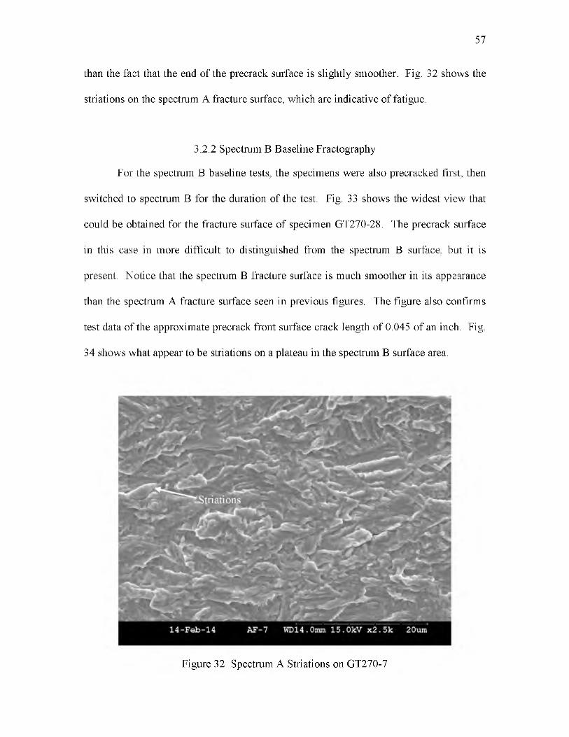
than the fact that the end of the precrack surface is slightly smoother. Fig. 32 shows the
striations on the spectrum A fracture surface, which are indicative of fatigue.
3.2.2 Spectrum B Baseline Fractography
For the spectrum B baseline tests, the specimens were also precracked first, then
switched to spectrum B for the duration of the test. Fig. 33 shows the widest view that
could be obtained for the fracture surface of specimen GT270-28. The precrack surface
in this case in more difficult to distinguished from the spectrum B surface, but it is
present. Notice that the spectrum B fracture surface is much smoother in its appearance
than the spectrum A fracture surface seen in previous figures. The figure also confirms
test data of the approximate precrack front surface crack length of 0.045 of an inch. Fig.
34 shows what appear to be striations on a plateau in the spectrum B surface area.
57
Figure 32 Spectrum A Striations on GT270-7
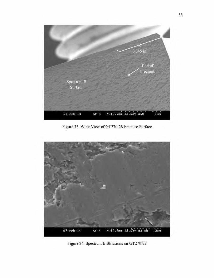
58
0.045 in
End of Precrack
Spectrum B Surface
07-Feb-14 AF-3 WD12.7mm 15!okV°x4o" ° ° lmm
Figure 33 Wide View of GT270-28 Fracture Surface
07-Feb-14 AF-4 WD12.8mm 15.0kV x3.0k lOum
Figure 34 Spectrum B Striations on GT270-28
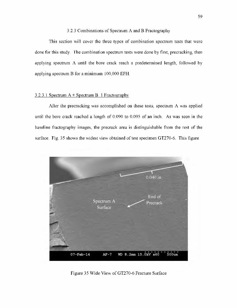
3.2.3 Combinations of Spectrum A and B Fractography
This section will cover the three types of combination spectrum tests that were
done for this study. The combination spectrum tests were done by first, precracking, then
applying spectrum A until the bore crack reach a predetermined length, followed by
applying spectrum B for a minimum 100,000 EFH.
3.2.3.1 Spectrum A + Spectrum B 1 Fractography
After the precracking was accomplished on these tests, spectrum A was applied
until the bore crack reached a length of 0.090 to 0.095 of an inch. As was seen in the
baseline fractography images, the precrack area is distinguishable from the rest of the
surface. Fig. 35 shows the widest view obtained of test specimen GT270-6. This figure
59
Figure 35 Wide View of GT270-6 Fracture Surface
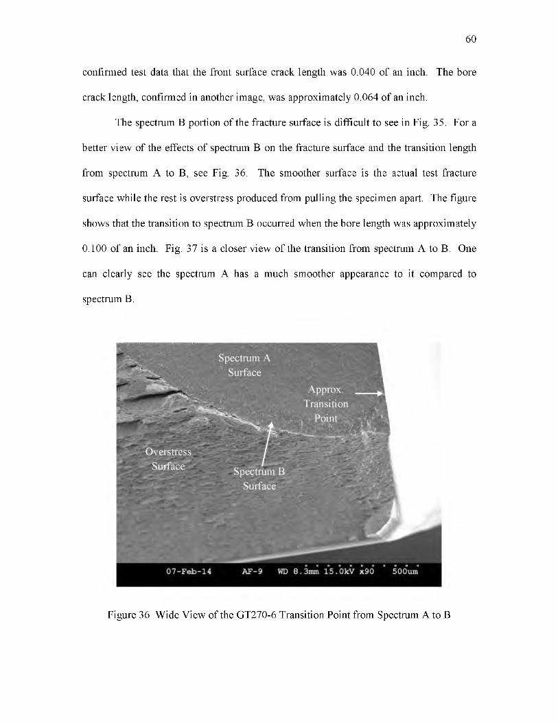
confirmed test data that the front surface crack length was 0.040 of an inch. The bore
crack length, confirmed in another image, was approximately 0.064 of an inch.
The spectrum B portion of the fracture surface is difficult to see in Fig. 35. For a
better view of the effects of spectrum B on the fracture surface and the transition length
from spectrum A to B, see Fig. 36. The smoother surface is the actual test fracture
surface while the rest is overstress produced from pulling the specimen apart. The figure
shows that the transition to spectrum B occurred when the bore length was approximately
0.100 of an inch. Fig. 37 is a closer view of the transition from spectrum A to B. One
can clearly see the spectrum A has a much smoother appearance to it compared to
spectrum B.
60
Figure 36 Wide View of the GT270-6 Transition Point from Spectrum A to B
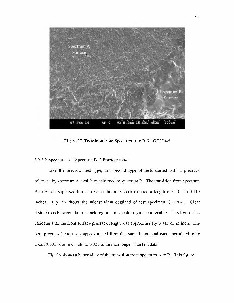
61
Figure 37 Transition from Spectrum A to B for GT270-6
3.2.3.2 Spectrum A + Spectrum B 2 Fractography
Like the previous test type, this second type of tests started with a precrack
followed by spectrum A, which transitioned to spectrum B. The transition from spectrum
A to B was supposed to occur when the bore crack reached a length of 0.105 to 0.110
inches. Fig. 38 shows the widest view obtained of test specimen GT270-9. Clear
distinctions between the precrack region and spectra regions are visible. This figure also
validates that the front surface precrack length was approximately 0.042 of an inch. The
bore precrack length was approximated from this same image and was determined to be
about 0.090 of an inch, about 0.020 of an inch longer than test data.
Fig. 39 shows a better view of the transition from spectrum A to B. This figure

62
07-Feb-14 AF-9 WD11.3mm 15.0kV x40 lmm
Figure 38 Wide View of GT270-9 Fracture Surface
Figure 39 Wide View of the GT270-9 Transition from Spectrum A to B
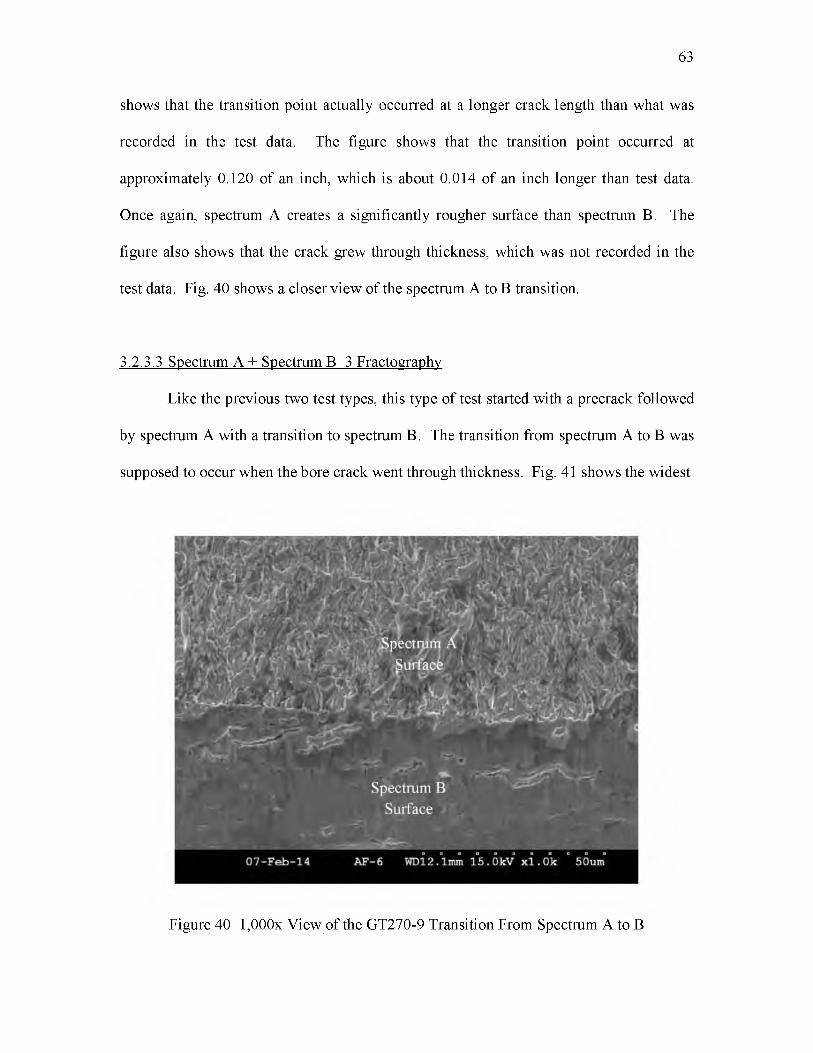
shows that the transition point actually occurred at a longer crack length than what was
recorded in the test data. The figure shows that the transition point occurred at
approximately 0.120 of an inch, which is about 0.014 of an inch longer than test data.
Once again, spectrum A creates a significantly rougher surface than spectrum B. The
figure also shows that the crack grew through thickness, which was not recorded in the
test data. Fig. 40 shows a closer view of the spectrum A to B transition.
3.2.3.3 Spectrum A + Spectrum B 3 Fractography
Like the previous two test types, this type of test started with a precrack followed
by spectrum A with a transition to spectrum B. The transition from spectrum A to B was
supposed to occur when the bore crack went through thickness. Fig. 41 shows the widest
63
Figure 40 1,000x View of the GT270-9 Transition From Spectrum A to B
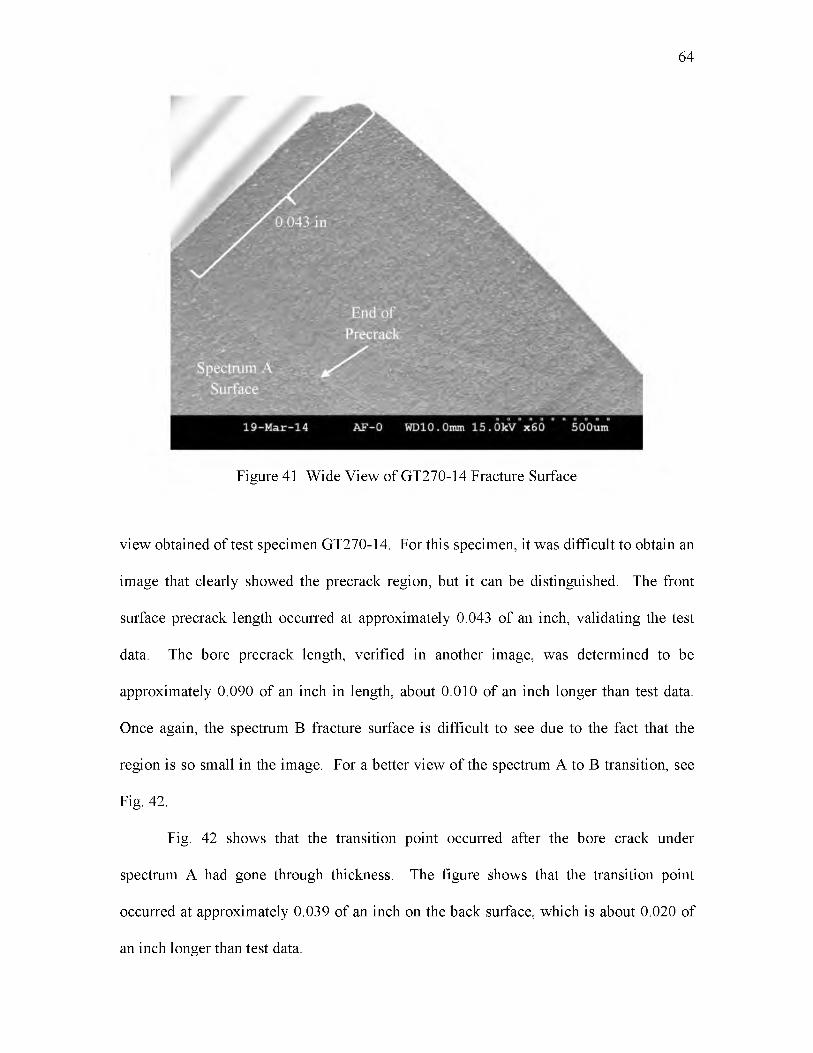
64
Figure 41 Wide View of GT270-14 Fracture Surface
view obtained of test specimen GT270-14. For this specimen, it was difficult to obtain an
image that clearly showed the precrack region, but it can be distinguished. The front
surface precrack length occurred at approximately 0.043 of an inch, validating the test
data. The bore precrack length, verified in another image, was determined to be
approximately 0.090 of an inch in length, about 0.010 of an inch longer than test data.
Once again, the spectrum B fracture surface is difficult to see due to the fact that the
region is so small in the image. For a better view of the spectrum A to B transition, see
Fig. 42.
Fig. 42 shows that the transition point occurred after the bore crack under
spectrum A had gone through thickness. The figure shows that the transition point
occurred at approximately 0.039 of an inch on the back surface, which is about 0.020 of
an inch longer than test data.

65
Figure 42 Wide View of the GT270-14 Transition from Spectrum A to B
3.3 AFGROW Simulations
This section shows the results of the AFGROW models developed to simulate the
test data gathered for each type of test. The 17-7PH data in the NASGRO material
database were used for most of these simulations. The TH1050 heat treatment condition
was used for the simulations because the specific heat treatment condition of the test
specimens was not available in the NASGRO database. No retardation models were used
in the development of these models. Note that all the simulations were done in such a
manner as to make them agree well with the test data and produce conservative results.
All initial crack lengths used in the simulations were approximations to the actual initial
crack lengths of the respective tests.
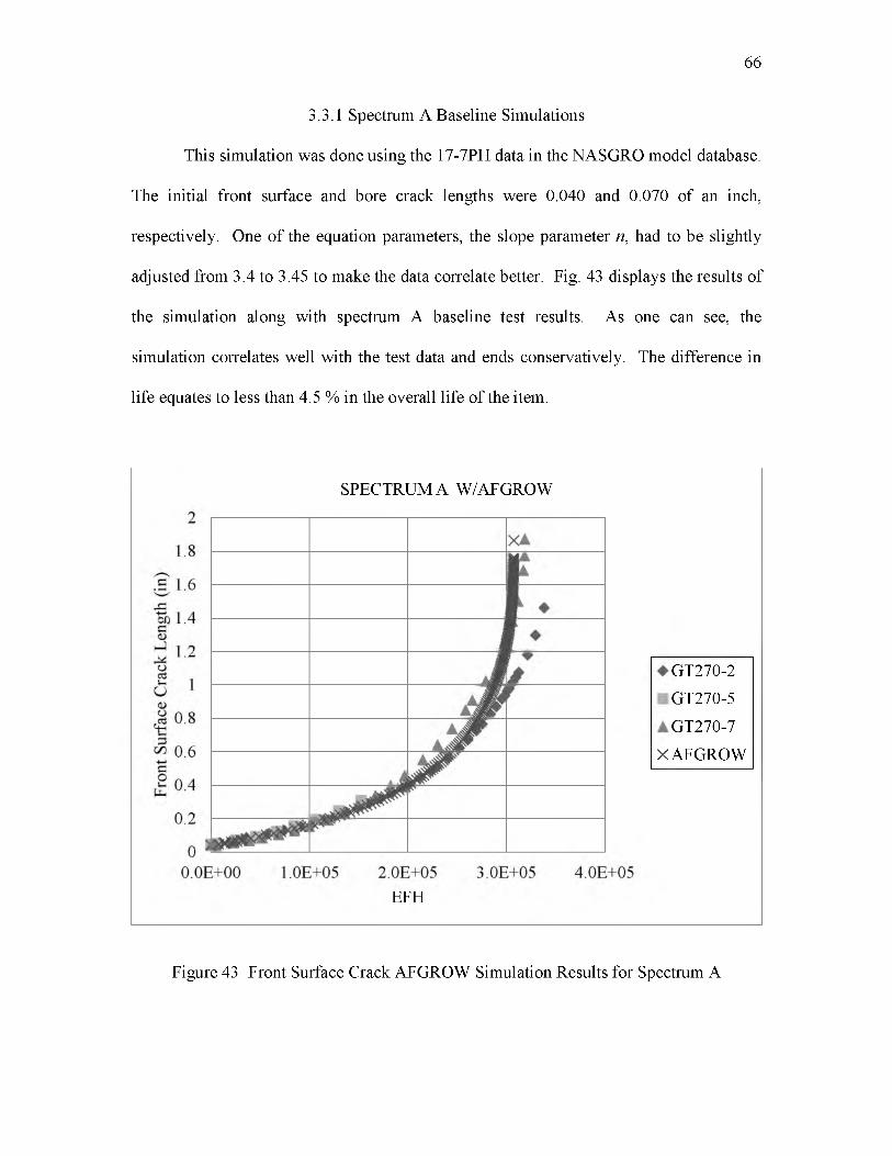
3.3.1 Spectrum A Baseline Simulations
This simulation was done using the 17-7PH data in the NASGRO model database.
The initial front surface and bore crack lengths were 0.040 and 0.070 of an inch,
respectively. One of the equation parameters, the slope parameter n, had to be slightly
adjusted from 3.4 to 3.45 to make the data correlate better. Fig. 43 displays the results of
the simulation along with spectrum A baseline test results. As one can see, the
simulation correlates well with the test data and ends conservatively. The difference in
life equates to less than 4.5 % in the overall life of the item.
66
SPECTRUM A W/AFGROW
EFH
GT270-2
GT270-5
GT270-7
X AFGROW
Figure 43 Front Surface Crack AFGROW Simulation Results for Spectrum A
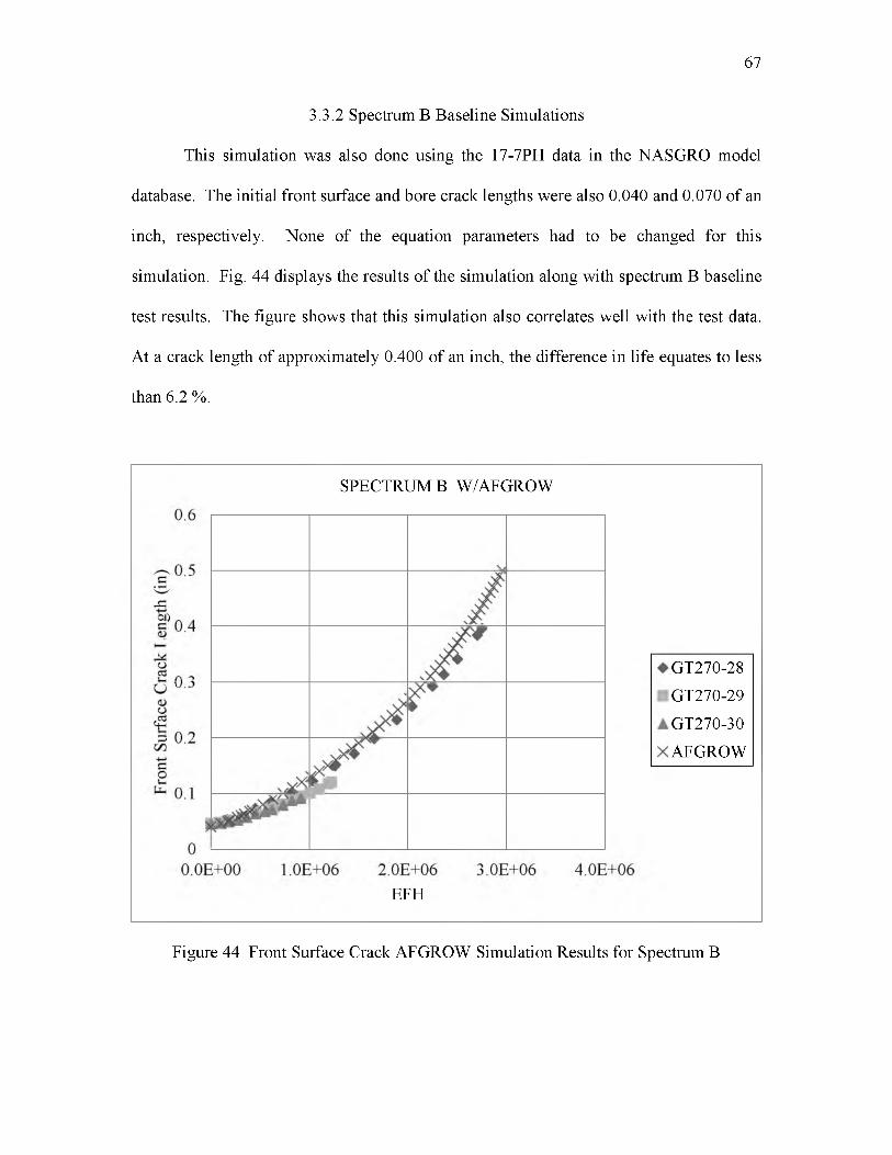
3.3.2 Spectrum B Baseline Simulations
This simulation was also done using the 17-7PH data in the NASGRO model
database. The initial front surface and bore crack lengths were also 0.040 and 0.070 of an
inch, respectively. None of the equation parameters had to be changed for this
simulation. Fig. 44 displays the results of the simulation along with spectrum B baseline
test results. The figure shows that this simulation also correlates well with the test data.
At a crack length of approximately 0.400 of an inch, the difference in life equates to less
than 6.2 %.
67
SPECTRUM B W/AFGROW
htgneLkcarCecafruStnorF
EFH
GT270-28
GT270-29
GT270-30
AFGROW
Figure 44 Front Surface Crack AFGROW Simulation Results for Spectrum B

3.3.3 Spectrum Combination Simulations
In this section, simulations for the front surface crack were developed. To match
the data for each type of combination, test two simulations were developed, one for the
spectrum A portion of the curve and the other for the spectrum B portion. Both the
spectrum A and B portions of the crack used the NASGRO database. In these
simulations, it was not necessary to change any of the NASGRO equation parameters.
For greater detail on how these simulations were developed, see section 4.3.1.
3.3.3.1 Spectrum A + Spectrum B 1 Simulation
The initial front surface and bore crack lengths used for this simulation were
0.040 and 0.070 of an inch, respectively. The transition to spectrum B occurred when the
front surface and bore crack lengths reached approximately 0.064 and 0.090 of an inch,
respectively. Fig. 45 displays the results of the simulation along with spectrum A + B_1
test results. This figure shows that the simulation correlated well with the test data.
3.3.3.2 Spectrum A + Spectrum B 2 Simulation
The initial front surface and bore crack lengths used for this simulation were
0.050 and 0.070 inches, respectively. The initial front surface crack length slightly
differs from that recorded for these specimens, but it was changed to better match the test
data. The transition to spectrum B occurred when the spectrum A portion of the
simulation reached a front surface and bore crack lengths of 0.088 and 0.110 of an inch,
respectively. Fig. 46 displays the results of the simulation along with spectrum A + B_2
test results. This figure also shows that the simulation correlated well with the test data.
68

69
0.09
^ 0.08
^ 0.07 a rCce 0.06acfr
^ 0.05 n
^ 0.04 1
n m
FRONT SURFACE A + B_1 W/AFGROW
A
♦ a ^ A
A |
■
1
t * ■
GT270-6
■ GT270-8
A AFGROW?wmi
;>►
0.0E+00 1.0E+05 2.0E+05 3.0E+05 4.0E+05EFH
Figure 45 Front Surface Crack Simulation Results for the A + B_1 Combination
FRONT SURFACE A + B 2 W/AFGROW
0.11
S 0.1
^ 0.09 n e^ 0.08 k
5 0.07
J 0.06 f ruS 0.05 t n
£ 0.04
0.030.0E+00 5.0E+04 1.0E+05 1.5E+05 2.0E+05
EFH
♦■
t 1+
4A
♦
/A
/mM*i i
w
GT270-9
■ GT270-10
A AFGROW
Figure 46 Front Surface Crack Simulation Results for the A + B_2 Combination

3.3.3.3 Spectrum A + Spectrum B 3 Simulation
The initial front surface and bore crack lengths used for this simulation were
0.050 and 0.070 of an inch, respectively. The initial front surface crack length again is
slightly different from that recorded for these specimens for the same reasoning as was
explained in the previous section. The transition to spectrum B occurred when the
spectrum A portion of the simulation reached a front surface and bore crack lengths of
0.080 and 0.102 of an inch, respectively. Fig. 47 displays the results of the simulation
along with spectrum A + B_3 test results. This simulation also correlated well with the
test data.
70
FRONT SURFACE A + B 3 W/AFGROW
0.11
0.1
^ 0.09 htg n
j 0.08
5 0.07 ec0.06ur
Se 0.05 o r F
0.04
0.030.0E+00 1.0E+05 2.0E+05 3.0E+05 4.0E+05 5.0E+05
EFH
♦
■
>v■
' ♦
■■
v
x x♦ A
x A A
2 AA
GT270-12
■ GT270-13
GT270-14
X AFGROW
Figure 47 Front Surface Crack Simulation Results for the A + B_3 Combination

CHAPTER 4
DISCUSSION
4.1 Observations of Spectra
This study was done to compare two spectra that were observed to occur at
different times in a fleet of aircraft. Data for spectrum A were gathered primarily during
the 1990s while data for spectrum B have been gathered from the early 2000s to the
present. Until testing is done on representative test specimens to compare the two
spectra, it is impossible to quantify how different the behaviors will be. It should be
noted that controlling the error on spectrum B was more difficult. The result was that
testing under spectrum B had to be run at slower speeds to minimize the error. Testing
actual coupons and developing analytical models from the data shows that the material in
the desired location on the aircraft, in this case 17-7PH, is predictable. For a similar
study using 2024-T351 aluminum, see reference [10]. The information obtained from
both the testing and analysis can then be utilized in the development of best maintenance
practices for the given loading condition.
4.1.1 Spectra Baseline
Baseline comparisons are essential for understanding what is occurring with the
different spectra. This section will go into more detail about each of the spectra

attributes. That will be followed by a more in-depth discussion about the test results.
The result will provide a better understanding about the basic and quantifiable differences
between the spectra.
4.1.1.1 Spectra Attributes
Based on the spectra attributes, which was seen in Table 4, one can deduce that
spectrum A was a more aggressive loading scenario than spectrum B. Spectrum A had
16,731 damage producing load points in a 240 EFH period. [8] In contrast to that,
spectrum B had only 4,371 damage producing load points in a 1000 EFH period. [8]
That means that spectrum A produces roughly four times the amount of load events in a
quarter of the time than that of spectrum B.
As far as the loads are concerned, the max and min loads for spectrum A are
10,977 lb and 99 lb, respectively. For spectrum B, the loads are 10,977 lb for the max
load and 133 lb for the min load. When the max load is applied to the test specimens,
with an average cross-sectional area of 0.500 in , it produces a max stress of 21.954 ksi, a
small fraction of the material capability in terms of yield strength. What does that mean
when applied to the actual aircraft? This next section will show a side-by-side
comparison of the test results.
4.1.1.2 Spectra Baseline Test Results Comparison
Fig. 48 is a plot directly comparing the front surface crack lengths results of the
baseline tests. The average initial front surface crack length for all of these specimens
was 0.046 of an inch. Since none of the spectrum B baseline tests were run to complete
72
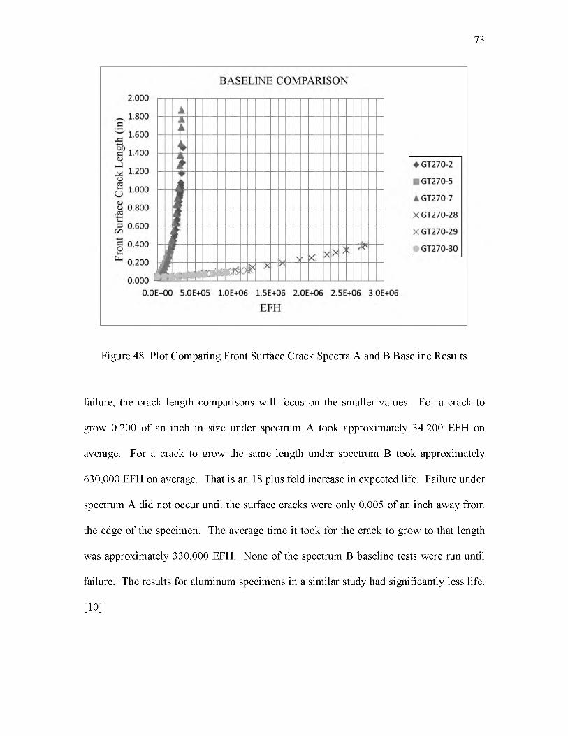
73
Figure 48 Plot Comparing Front Surface Crack Spectra A and B Baseline Results
failure, the crack length comparisons will focus on the smaller values. For a crack to
grow 0.200 of an inch in size under spectrum A took approximately 34,200 EFH on
average. For a crack to grow the same length under spectrum B took approximately
630,000 EFH on average. That is an 18 plus fold increase in expected life. Failure under
spectrum A did not occur until the surface cracks were only 0.005 of an inch away from
the edge of the specimen. The average time it took for the crack to grow to that length
was approximately 330,000 EFH. None of the spectrum B baseline tests were run until
failure. The results for aluminum specimens in a similar study had significantly less life.
[10]
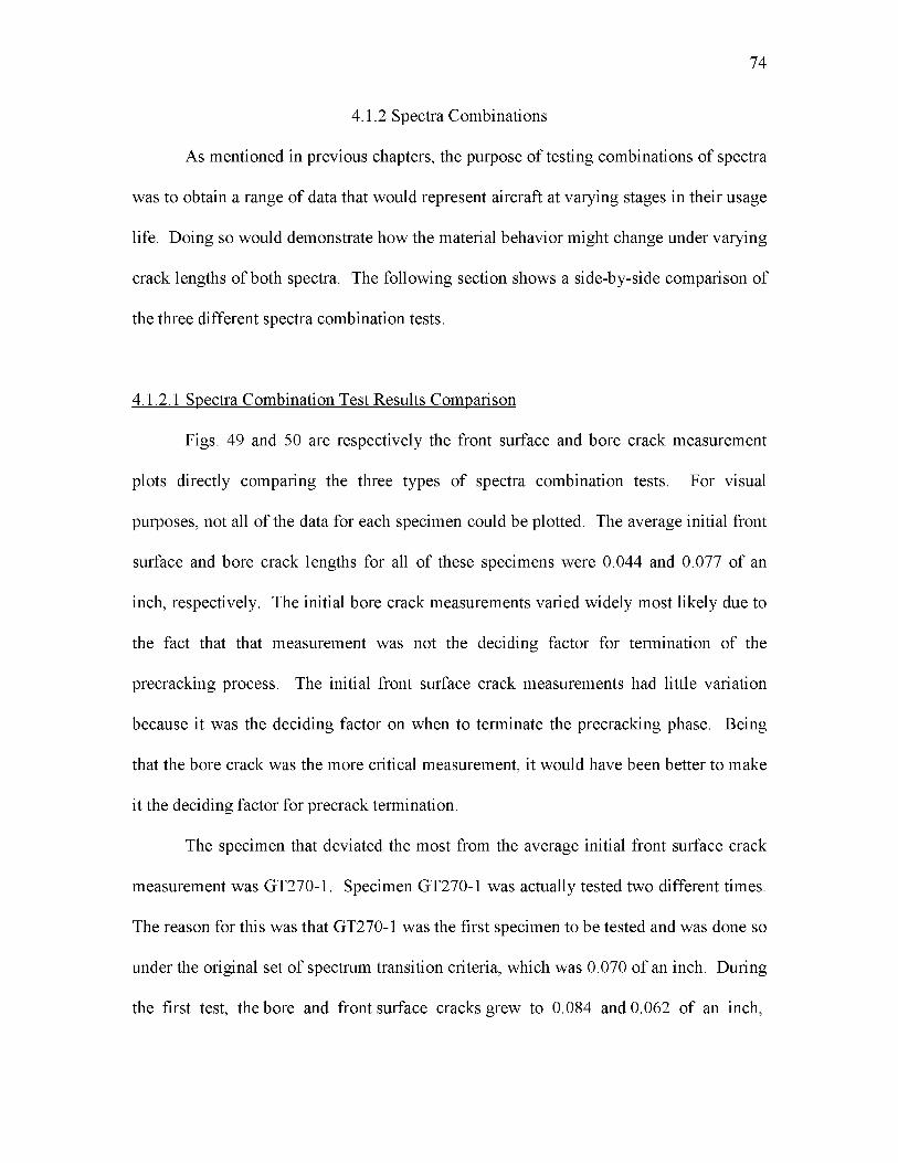
74
4.1.2 Spectra Combinations
As mentioned in previous chapters, the purpose of testing combinations of spectra
was to obtain a range of data that would represent aircraft at varying stages in their usage
life. Doing so would demonstrate how the material behavior might change under varying
crack lengths of both spectra. The following section shows a side-by-side comparison of
the three different spectra combination tests.
4.1.2.1 Spectra Combination Test Results Comparison
Figs. 49 and 50 are respectively the front surface and bore crack measurement
plots directly comparing the three types of spectra combination tests. For visual
purposes, not all of the data for each specimen could be plotted. The average initial front
surface and bore crack lengths for all of these specimens were 0.044 and 0.077 of an
inch, respectively. The initial bore crack measurements varied widely most likely due to
the fact that that measurement was not the deciding factor for termination of the
precracking process. The initial front surface crack measurements had little variation
because it was the deciding factor on when to terminate the precracking phase. Being
that the bore crack was the more critical measurement, it would have been better to make
it the deciding factor for precrack termination.
The specimen that deviated the most from the average initial front surface crack
measurement was GT270-1. Specimen GT270-1 was actually tested two different times.
The reason for this was that GT270-1 was the first specimen to be tested and was done so
under the original set of spectrum transition criteria, which was 0.070 of an inch. During
the first test, the bore and front surface cracks grew to 0.084 and 0.062 of an inch,
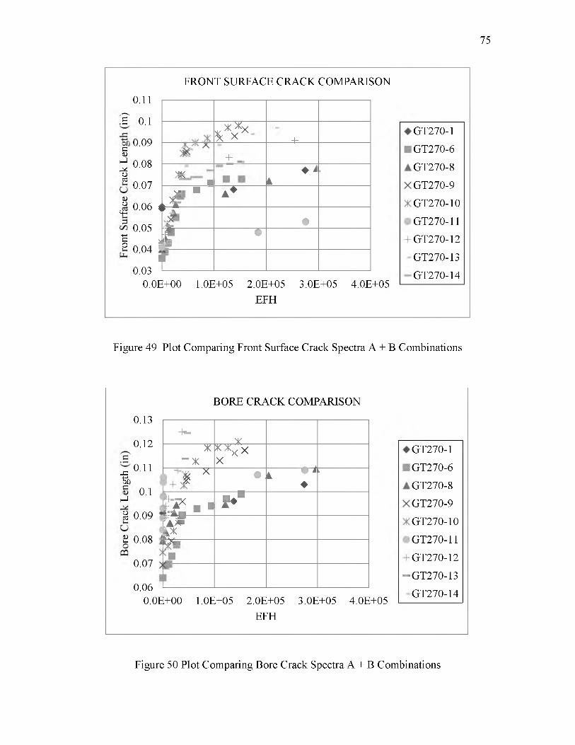
75
FRONT SURFACE CRACK COMPARISON
0.11
? 0.1
0.09
0.08
0.07
0.06
0.05
0.04
0.03
c(Uh-lMocS
C(Uo4-H
3S- Mco
F
^ x - ++ _
\M/ ■ ♦ ik■X*'
-----<
A *
u *•
Jf •
f
0.0E+00 1.0E+05 2.0E+05 3.0E+05 4.0E+05EFH
GT270-1
GT270-6
GT270-8
GT270-9
GT270-10
GT270-11
GT270-12
-GT270-13
GT270-14
Figure 49 Plot Comparing Front Surface Crack Spectra A + B Combinations
BORE CRACK COMPARISON
0.13
0.12
M 011 1&
en 0.1h-I
k£ 0.09 r
C£ 0.08 o
B0.07
0.06
-1— XX“X **>?xX% x • k 9 * ♦
i
jjg -« f "£
U
0.0E+00 1.0E+05 2.0E+05 3.0E+05 4.0E+05EFH
GT270-1
GT270-6
GT270-8
GT270-9
GT270-10
GT270-11
GT270-12
— GT270-13
GT270-14
Figure 50 Plot Comparing Bore Crack Spectra A + B Combinations
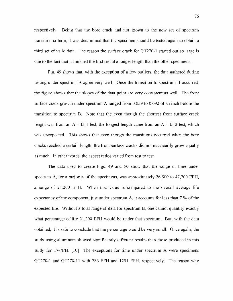
respectively. Being that the bore crack had not grown to the new set of spectrum
transition criteria, it was determined that the specimen should be tested again to obtain a
third set of valid data. The reason the surface crack for GT270-1 started out so large is
due to the fact that it finished the first test at a longer length than the other specimens.
Fig. 49 shows that, with the exception of a few outliers, the data gathered during
testing under spectrum A agree very well. Once the transition to spectrum B occurred,
the figure shows that the slopes of the data point are very consistent as well. The front
surface crack growth under spectrum A ranged from 0.059 to 0.092 of an inch before the
transition to spectrum B. Note that the even though the shortest front surface crack
length was from an A + B_1 test, the longest length came from an A + B_2 test, which
was unexpected. This shows that even though the transitions occurred when the bore
cracks reached a certain length, the front surface cracks did not necessarily grow equally
as much. In other words, the aspect ratios varied from test to test.
The data used to create Figs. 49 and 50 show that the range of time under
spectrum A, for a majority of the specimens, was approximately 26,500 to 47,700 EFH,
a range of 21,200 EFH. When that value is compared to the overall average life
expectancy of the component, just under spectrum A, it accounts for less than 7 % of the
expected life. Without a total range of data for spectrum B, one cannot quantify exactly
what percentage of life 21,200 EFH would be under that spectrum. But, with the data
obtained, it is safe to conclude that the percentage would be very small. Once again, the
study using aluminum showed significantly different results than those produced in this
study for 17-7PH. [10] The exceptions for time under spectrum A were specimens
GT270-1 and GT270-11 with 286 EFH and 1291 EFH, respectively. The reason why
76

Specimen GT270-1 spent so little time under spectrum A can be attributed to what was
discussed in the previous paragraph. The testing for specimen GT270-11 was conducted
at SwRI and they did not mention any anomalies that occurred during testing. Therefore,
it is unclear why that particular specimen’s test results deviated from the other test data.
Due to the uncertainty of the results from these two specimens, the data were not used in
further analyses.
Fig. 50 shows that even though the initial bore crack lengths varied significantly,
the transition crack lengths were as specified for each type of test. The range of initial
bore crack lengths was 0.064 to 0.084 of an inch. Once again, it is important to
remember that those are initial values, which highlights the variations that occurred
during precracking.
4.2 Observations from Fractographic Examinations
The main observation that came from the fractography images of the baseline
specimen was how different the appearances were between the two spectra. Spectrum A,
as was seen most of the fractography images, had a consistently rougher appearance.
Even though striations could be seen on both spectrum A and B fracture surfaces, they
were much easier to see on spectrum A fracture surfaces.
In contrast to spectrum A, fracture surfaces produced by spectrum B had a
significantly smoother appearance. Another interesting phenomenon that was observed
initially in some of the spectrum B fracture surface was the appearance of cracks that
formed in the L-T plane of the specimens; see Figs. 51 and 52. These cracks were seen
preferentially in the middle range of the thickness. As was stated in Chapter 2 these
77
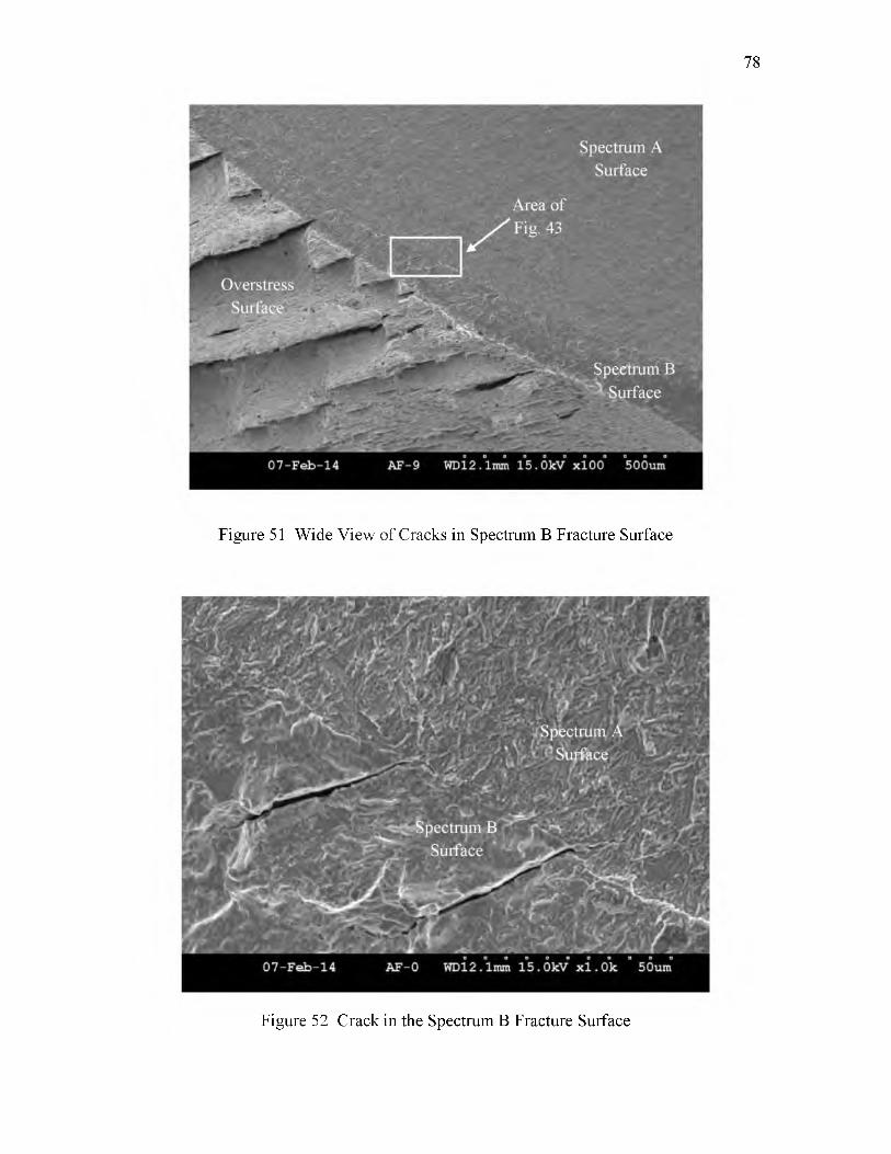
78
Figure 51 Wide View of Cracks in Spectrum B Fracture Surface
Figure 52 Crack in the Spectrum B Fracture Surface
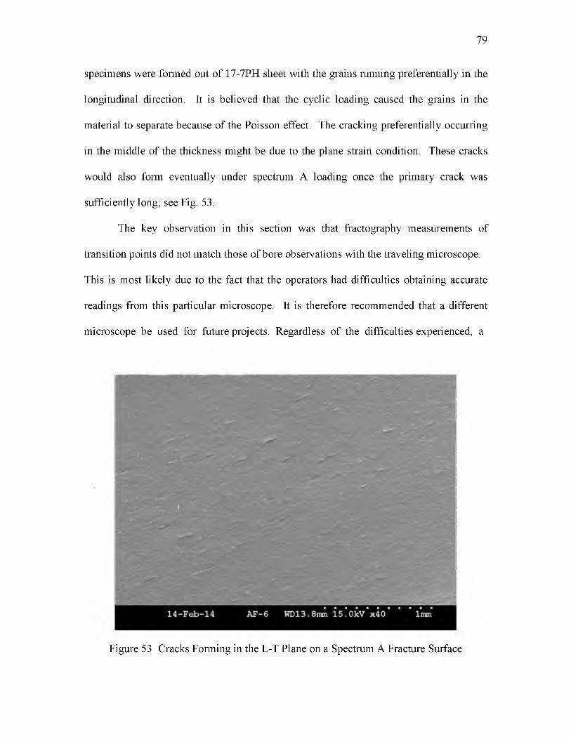
specimens were formed out of 17-7PH sheet with the grains running preferentially in the
longitudinal direction. It is believed that the cyclic loading caused the grains in the
material to separate because of the Poisson effect. The cracking preferentially occurring
in the middle of the thickness might be due to the plane strain condition. These cracks
would also form eventually under spectrum A loading once the primary crack was
sufficiently long; see Fig. 53.
The key observation in this section was that fractography measurements of
transition points did not match those of bore observations with the traveling microscope.
This is most likely due to the fact that the operators had difficulties obtaining accurate
readings from this particular microscope. It is therefore recommended that a different
microscope be used for future projects. Regardless of the difficulties experienced, a
79
Figure 53 Cracks Forming in the L-T Plane on a Spectrum A Fracture Surface
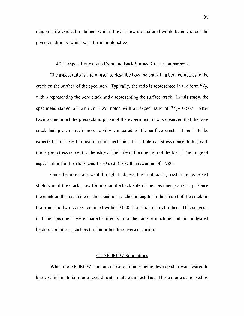
range of life was still obtained, which showed how the material would behave under the
given conditions, which was the main objective.
4.2.1 Aspect Ratios with Front and Back Surface Crack Comparisons
The aspect ratio is a term used to describe how the crack in a bore compares to the
crack on the surface of the specimen. Typically, the ratio is represented in the form a/ c,
with a representing the bore crack and c representing the surface crack. In this study, the
specimens started off with an EDM notch with an aspect ratio of a/ c= 0.667. After
having conducted the precracking phase of the experiment, it was observed that the bore
crack had grown much more rapidly compared to the surface crack. This is to be
expected as it is well known in solid mechanics that a hole is a stress concentrator, with
the largest stress tangent to the edge of the hole in the direction of the load. The range of
aspect ratios for this study was 1.370 to 2.018 with an average of 1.789.
Once the bore crack went through thickness, the front crack growth rate decreased
slightly until the crack, now forming on the back side of the specimen, caught up. Once
the crack on the back side of the specimen reached a length similar to that of the crack on
the front, the two cracks remained within 0.020 of an inch of each other. This suggests
that the specimens were loaded correctly into the fatigue machine and no undesired
loading conditions, such as torsion or bending, were occurring.
4.3 AFGROW Simulations
When the AFGROW simulations were initially being developed, it was desired to
know which material model would best simulate the test data. These models are used by
80
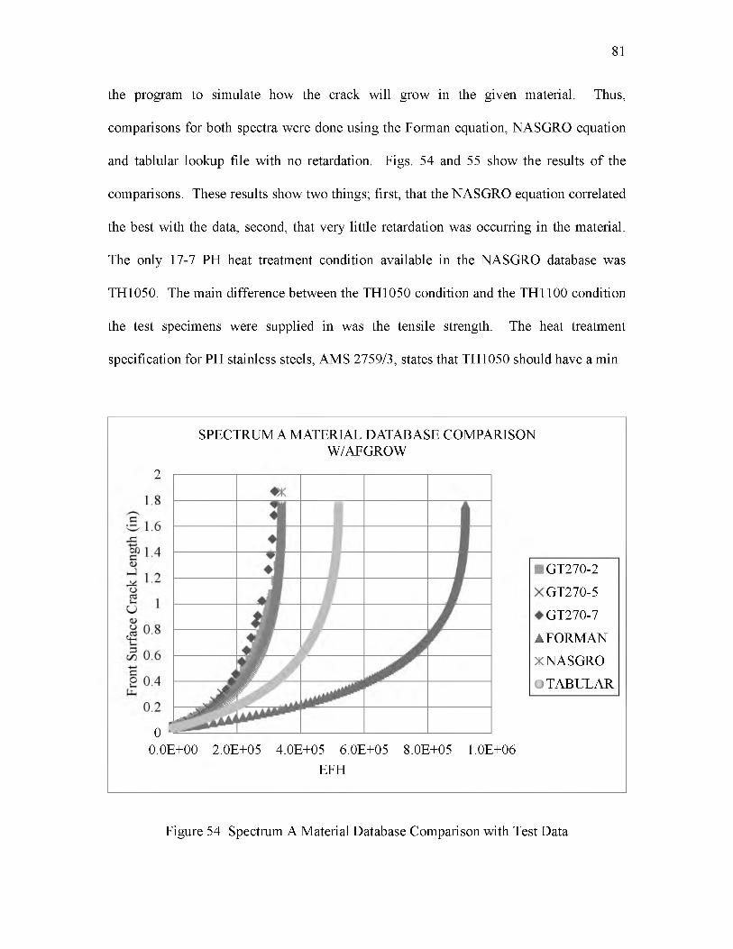
81
the program to simulate how the crack will grow in the given material. Thus,
comparisons for both spectra were done using the Forman equation, NASGRO equation
and tablular lookup file with no retardation. Figs. 54 and 55 show the results of the
comparisons. These results show two things; first, that the NASGRO equation correlated
the best with the data, second, that very little retardation was occurring in the material.
The only 17-7 PH heat treatment condition available in the NASGRO database was
TH1050. The main difference between the TH1050 condition and the TH1100 condition
the test specimens were supplied in was the tensile strength. The heat treatment
specification for PH stainless steels, AMS 2759/3, states that TH1050 should have a min
SPECTRUM A MATERIAL DATABASE COMPARISON W/AFGROW
2
00.0E+00 2.0E+05 4.0E+05 6.0E+05 8.0E+05 1.0E+06
EFH
GT270-2
GT270-5
GT270-7
A FORMAN
X NASGRO
•TA B U LA R
Figure 54 Spectrum A Material Database Comparison with Test Data

82
0.6
0.5
0.4c
ouOo
GO
GO£ 0
SPECTRUM B MATERIAL DATABASE COMPARISON W/AFGROW
•
xxX xX "yX
<XX
y ^ X xA
00.0E+00 2.0E+06 4.0E+06 6.0E+06
EFH8.0E+06 1.0E+07
GT270-28
GT270-29
GT270-30
X FORMAN
X NASGRO
•TA B U LA R
Figure 55 Spectrum B Material Database Comparison with Test Data
tensile strength of 180 ksi. [32] The average test specimen tensile strength was
approximately 170 ksi, making the difference between the two conditions 10 ksi. Though
the heat treatment condition in the NASGRO database differed from that of the actual test
specimens, the predictions agreed very well with the test data.
The NASGRO equation uses material properties and a mathematical model to
predict crack growth for a given material. The following is the NASGRO equation used
in AFGROW. [30]
83
= c \ t 1 - ^ . l ” ( l — STf )̂/■i - A l " ( 1(H ? H r
AKr ' v Ah
( l — Kmax\ Q
Kcrit'
where ^ a/^ N is the crack growth rate; C, n, p, and q are empirically derived parameters,
f is the ratio of Kopover Kmax and R is the stress ratio. As mentioned previously, n was
slightly increased from 3.4 to 3.45 because increasing the slope made the prediction
conservative and conforms better to test data. See the AFGROW Users Guide for further
details. [30]
The fact that very little retardation is occurring during testing is evident from the
simulations. Most materials will experience some retardation when an overload occurs in
the loading sequence. The degree o f retardation will vary depending on the material
being used and the degree o f the overload. The degree o f retardation observed in this
study appears to be very little. For this reason, in order to obtain the best fit to the test
data, no retardation models were used.
4.3.1 Spectra Combination Simulations
To match the data for each type o f combination test, two simulations were
developed, one for the spectrum A portion of the curve and the other for the spectrum B
portion. This was done by running the spectrum A portion o f the simulation until the
transition point matched that of the test data. The spectrum B portion of the test was then
simulated using the new front surface and bore crack lengths produced from the spectrum
A portion of the simulation. The results of the two simulations were then combined in an
Excel spreadsheet. Note that the aspect ratios o f these simulations did not necessarily
match that of the test data. These efforts focused on representing the front surface crack.

In these simulations, it was not necessary to change any of the NASGRO equation
parameters. The main difference between the two portions of the crack simulation was
that, to better match the spectrum A portion of the curve, the aspect ratios were not forced
to remain constant, which was not done for the spectrum B portion.
84

CHAPTER 5
CONCLUSIONS AND RECOMMENDATIONS
5.1 Conclusions
The main objective of this study was to better understand the sensitivity of 17
7PH to the different spectra. The crack growth curves, fractographic examinations and
AFGROW simulations provided the information necessary for users of this aircraft to
better maintain the integrity of the structure. The following sections detail the
conclusions obtained from each of those analyses performed. Now that a better
understanding of the differences between the two spectra has been obtained, engineers
can make alterations, based on the damage tolerant design philosophy, to maintenance
practices, repair procedures and inspection intervals. This study showed that while the
aircraft are under spectrum B type conditions, the component, in the location studied, will
last for hundreds of thousands of effective flight hours. The alterations in procedures will
reduce costs by eliminating unnecessary maintenance hours and inspections while
maintaining the integrity of the aircraft.
5.1.1 Crack Growth Curve Conclusions
The main takeaway from the crack growth curves is the degree to which the two
spectra differ. Before this study was conducted, the differences in crack growth behavior
between spectra A and B were suspected but unvalidated. It is now known that usage,
under spectrum B type conditions, is much more benign than that of spectrum A. Again,
for a crack to grow 0.200 of an inch under spectrum B takes 18 times as long as spectrum
A. The combination tests showed that once the transition to spectrum B occurred, it
dominated in all cases. Thus, no matter what stage in life the aircraft may be in, if the
usage for that aircraft is spectrum B type conditions, the respective component’s integrity
will not be compromised before inspections can occur.
5.1.2 Fractographic Examination Conclusions
The fractographic examinations showed some distinct feature differences between
the two spectra and the material itself. Spectrum A produced a fracture surface that had a
significantly rougher appearance than that of spectrum B. Another key feature that was
distinct for this material was the secondary cracks that formed in the fracture surface,
preferentially in the middle thickness section. These cracks were predominately observed
in the spectrum B fracture surface, but could be seen in the spectrum A fracture surface if
the primary crack was sufficiently long. These examinations also showed that the bore
crack measurements taken during the testing were not accurate, being off as much as
0.020 of an inch. Even though these inaccuracies occurred, the main objective of
obtaining a range of life was achieved, the results of which were discussed in the
previous section. The last observation obtained from the examinations has to do with the
aspect ratios. The fatigue tests provided a wide range of aspect ratios, which complicated
crack growth simulations.
86
5.1.3 AFGROW Simulation Conclusions
Simulations of crack growth for the 5 different types of tests were obtained. The
NASGRO database, for 17-7PH, produced the best results of the different material
databases. Initial simulations indicate that very little retardation of the crack growth
occurred during testing. For the spectrum A baseline simulation, the n parameter had to
be slightly adjusted from 3.4 to 3.45 to obtain a better fit. As far as the combination tests
were concerned, the aspect ratios, for the spectrum A portion of the simulation, were not
forced to remain constant to, once again, obtain a better fit. Also, the initial front surface
crack size had to be slightly increased to 0.050 of an inch from 0.040 of an inch for the A
+ B_2 and A + B_3 simulations. Doing so was necessary to better approximate the test
data.
5.2 Recommendations
The recommendations have been separated into the three following sections: test
practices, potential future studies and current aircraft.
5.2.1 Test Practices
When preparing to perform a fatigue test, it is recommended that the operators
take time to better understand and inspect the major components of the machine. During
this study, the fatigue machine failed due to a hydraulic pump failure. If the pump had
been inspected prior to testing, the deficiency may have been caught early and
unnecessary delays would not have occurred. This was also true for the microscope that
gave inaccurate measurements. Though those performing the testing had difficulty with
the microscopes it was not known, until the fractographic examinations, that the
87
measurements were inaccurate. Also, knowing the limitations of the machine will reduce
the amount of error that can occur. In some instances, during this study, the loading rate
was increased to accelerate the testing. Though the error remained within acceptable
limits, it would have been better to continue with the reduced loading rate to better
maintain the error
5.2.2 Potential Future Studies
It is recommended that fatigue-prone systems, like aircraft, be continually
monitored for failures. Loading conditions need to be observed, especially if usage has
changed from that for which the system has been previously tested. Significant changes
in usage should then be fatigue tested, as was done in this study, to determine the
sensitivity of the materials in question to the changes in usage. From the data obtained,
engineers can develop better models, based on the damage tolerant design philosophy,
which empower them to make better determinations on how maintenance practices can be
applied. As mentioned earlier, these types of studies can save time and money for the
user by developing the more efficient maintenance practices while maintaining the
integrity of the system and prolonging its life.
5.2.3 Current Aircraft
Though the specific aircraft for this study was not mentioned, in order to
generalize the study, it is recommended that the maintenance practices be adjusted
appropriately based on the information given here in. It is now known that, while usage
of the aircraft are spectrum B type conditions, the respective area on the aircraft will last
88

significantly longer than when usage conditions more closely resemble that of spectrum
A. Depending on the relationship between the normal usage and the alternative usage,
this may provide economical relief to the operator while maintaining flight safety.
89

APPENDIX A
TEST SPECIMEN FABRICATION PROCEDURES AND MATERIAL
CERTIFICATION SHEETS
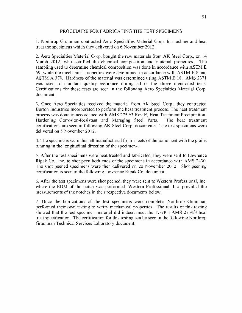
91
PROCEDURE FOR FABRICATING THE TEST SPECIMENS
1. Northrop Grumman contracted Aero Specialties Material Corp. to machine and heat treat the specimens which they delivered on 6 November 2012.
2. Aero Specialties Material Corp. bought the raw materials from AK Steel Corp., on 14 March 2012, who certified the chemical composition and material properties. The sampling used to determine chemical composition was done in accordance with ASTM E 59, while the mechanical properties were determined in accordance with ASTM E 8 and ASTM A 370. Hardness of the material was determined using ASTM E 18. AMS 2371 was used to maintain quality assurance during all of the above mentioned tests. Certifications for these tests are seen in the following Aero Specialties Material Corp. document.
3. Once Aero Specialties received the material from AK Steel Corp., they contracted Burton Industries Incorporated to perform the heat treatment process. The heat treatment process was done in accordance with AMS 2759/3 Rev E, Heat Treatment Precipitation- Hardening Corrosion-Resistant and Maraging Steel Parts. The heat treatment certifications are seen in following AK Steel Corp. documents. The test specimens were delivered on 5 November 2012.
4. The specimens were then all manufactured from sheets of the same heat with the grains running in the longitudinal direction of the specimens.
5. After the test specimens were heat treated and fabricated, they were sent to Lawrence Ripak Co., Inc. to shot peen both ends of the specimens in accordance with AMS 2430. The shot peened specimens were then delivered on 20 November 2012. Shot peening certification is seen in the following Lawrence Ripak Co. document.
6. After the test specimens were shot peened, they were sent to Western Professional, Inc. where the EDM of the notch was performed. Western Professional, Inc. provided the measurements of the notches in their respective documents below.
7. Once the fabrications of the test specimens were complete, Northrop Grumman performed their own testing to verify mechanical properties. The results of this testing showed that the test specimen material did indeed meet the 17-7PH AMS 2759/3 heat treat specification. The certification for this testing can be seen in the following Northrop Grumman Technical Services Laboratory document.

92
N o rth ro p G rum m an C orpora tion Technical Services925 South Oyster Bay Road -M/S UG3-26Bethpagc, New York 11714Tel: 516-575-3073; Fax: 516-575-9909
To: Michael BehringFrom: Robert Fidnarick / Ken Grube
Subject:Coupon Drawing GT270KB003-13, Coupons 1-33
Enclosures:1) Drawing GT270KB0032) Aero Specialties Material Corp Packing Slip with Material and Heat Treatment Certification for 17-7PH 150-170 ksi3) Technical Service Laboratory Material Property Report4) Lawrence Ripak Co. Inc Shot Peen Certification5) Western Professional EDM notch data sheet with Memo for Coupon 36) Technical Service Laboratory Coupon Measurements

93
Bill To:
NORTHROP GRUMMAN 925 SO. OYSTER BAY ROAD M/S U03-26 BETHPAGE.NY 11714
Ship to:
NORTHROP GRUMMAN TECH SVC. 925 SOUTH OYSTER BAY ROAD ATT: KEVIN COOK BETHPAGE.NY 11714
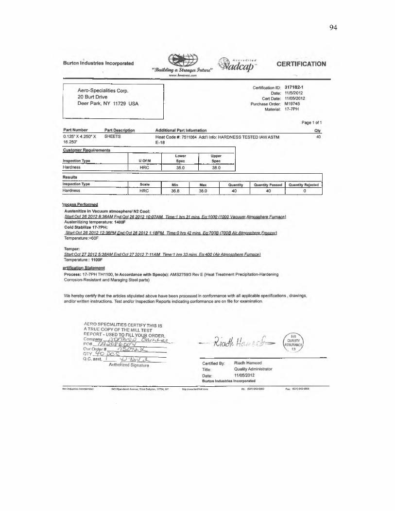
94
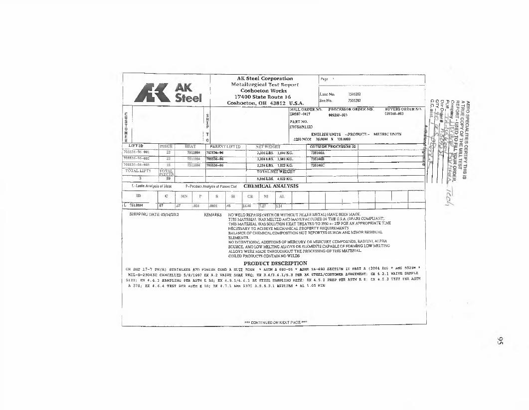
x c Steel
L IF T ID
7 0 5 536-06-001
705536 -0 6 -0 0 2
705536 -0 6 -0 0 3
T O T A L L IF T S T O T A L.PIECES.
AK S tee l C orpora tion M etallu rg ical Test R eport
C oshocton W orks 17400 S ta te R oute 16
C oshocton , OH 43812 U.S.A.
Page !
Load No.
S rn N o.
7503282
7503282
M IL L O R D ER NO. '230987-0417
PA R T NO. 1707SAN112D
PRO CESSO R O R D E R NO.
009260-003
BUYERS ORD ER NO. 009260-003
E N G LISH UNITS - :P R O I)U C T :- M E T R IC UNITS .1250 NOM 36,0000 X 120.0000
ODO"OO^j>> 0 ^ 2 3 ? ] h m“■USI ^
U r-̂ cn "O —
Rho o c
PA R E N T LIF T ID
705536-06
N E T W EIG H T
3,306 LBS. 1,500 K G .
3,306 LBS. 1,500 K G .
2,254 LBS. 1,022 KG.
TO TA L N ET W E IG H T
8,866 LBS. 4.022K G .
O U T SID E PRO CESSO R ID
L- Ladle Analysis of H eat P-Produci Analysis of Parent Coil CHEMICAL ANALYSIS
L 7513084 .07 67 .45 16.68 7.27 1.14
SHIPPING DATE: 03/14/2012 REMARKS NO W ELD REPAIRS (W ITH OR W ITH O U T FILLER METAL) HAVE BEEN MADE.THIS MATERIAL WAS MELTED AND MANUFACTURED IN T H E U.S-A. (DFARS COMPLIANT).THIS MATERIAL WAS SOLUTION H EA T TREATED TO 1950 + - 25F FOR AN APPROPRIATE TIME NECESSARY TO ACHIEVE MECHANICAL PROPERTY REQUIREMENTS.BALANCE O F CHEMICAL COMPOSITION N O T REPORTED IS IRON AND MINOR RESIDUAL ELEMENTS.NO INTENTIONAL ADDITIONS OF MERCURY OR MERCURY COMPOUNDS, RADIUM, ALPHA SOURCE. AND LOW MELTING ALLOYS OR ELEMENTS CAPABLE OF FORMING LOW MELTING ALLOYS W ERE MADE THROUGHOUT T H E PROCESSING O F THIS MATERIAL COILED PRODUCTS CONTAIN NO WELDS
PRODUCT DESCRIPTIONCR SHT 1 7 - 7 P H (R ) ST A IN L ESS #2D F IN IS H COND A S L IT EDGE * ASTM A 6 9 3 - 0 6 * ASME S A -6 9 3 SECTION I I PART A (2 0 0 4 £D ) * AMS 55 2 8 H *
M I L - S - 2 5 0 4 3 C CANCELLED 5 / 9 / 1 9 9 7 EX 3 . 2 WAIVE SOAK REQ; EX 3 . 6 / 3 . 6 . 1 / 5 . 3 PER AK STEEL/CUSTOMER AGREEMENT; EX 4 . 3 . 1 WAIVE SAMPLE S I Z E ; EX 4 . 4 . 1 SAMPLING PER ASTM E 5 9 ; EX 4 . 5 . 1 / 4 . 6 . 1 AK STEEL SAMPLING METH; EX 4 . 5 , 2 PREP PER ASTM E 8 ; EX 4 . 5 . 3 TEST PER ASTM
A 3 7 0 ; EX 4 . 6 . 4 TEST PER ASTM E 1 8 ; EX 4 . 7 . 1 AMS 2 3 7 1 3 . 3 . 5 . 3 .1 A PPL IES * AL 1 . 0 5 MIN
* CONTINUED ON NEXT PAGE *
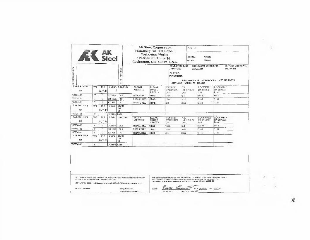
JEC Stee3
AK Steel C orporation M eta llu rg ical Test R epo rt
C oshocton W orks 17400 S ta te R oute 16
C oshocton , OH 43812 U.S.A.
Page 2
L oad No.
S rti No.
7503282
7503282
P R O C E SSO R O R D E R N O .
009260-003
BUYERS ORD ER NO. 009250-003
M IL L ORD ER NO- 230987-0417
P A R T NO.1707SAN112D
ENG LISH UNITS -.P R O D U C T :- M E T R IC UNITS .1250 NOM 36.0000 X 120.0000
P A R E N T L IF T
ID
P O S D IR
(L, T , D)
C O N D % ELO N G ELO N GM E T H O D
ELONGGAU GELENG TH
TEN SILESTREN G TH(KSI)
Y.S..2% O FFSE T (Ksr>
R O C K W ELLHARDN ESSTail
R O C K W E L LH ARDN ESSF ro n t
705536-06 T T C O N D A 36.6 M EA SU R ED 2 Inch 121.5 45.0 B W 88 BW 87705536-06 T T TH 1050 9.0 M EA SU R ED 2 In c h 199.6 191.0 C 45 C 44705536-06 T T RFI 950 7.7 M EA SU R ED 2 Inch 232 195.9 C 51 C 50
P A R E N T L IF T
ID
P O S D IR
(L, T, D)
COND BEND180IT
705536-06 T C O N D A PASSP A R E N T L IF T
ID
P O S DIR
a , t , d )
C O N D ■ % ELON G ELO N GM E T H O D
ELONGGAUGELEN G TH
TEN SIL ESTREN G TH(K SI)
Y ,s,.1% O FFSET (KSI)
RO C K W ELLHARDN ESSTail
R O C K W E L LH ARDN ESSF ro n t
705536-06 F T C O N D A 35.6 M EA SU RED 2 Inch 123.6 4 53 BW 88 BW 87
7 05 5 3 6 -0 6 F T TH 1050 10.4 M EA SU R ED 2 Inch 198.4 186.4 C 45 C 44
7 0 5 5 3 6 -0 6 F T R H 950 7.1 M E A SU R E D 2 Inch 231 203.0 C 51 C 50P A R E N T L IF T
ID
PO S DIR
(L, T, D)
C OND BEND180IT
7 05536-06 F C O N D A PASS
THE CKEVJCAL ANALYSE AND PHYSICAL OR MECHANICAL TSSTS ABOVE ARE'CORK EOTAS CO!\'TAlh4EE IN THE RECORDS OF THE OOaBSMA'TJCW.
ALL TESTING IS DON2. IM ACCCRQANOi WfTH AS-T.V- STANDARDS UNLESS OTHERWISE NOTED
AK S r j;i C jiporKicr:
Ffcgratn te rian i L.M43SB l . l t
THE CCBTIFO TliSTRSFCR? K*iS BEEN DELIVERED TO A CONSIGNEE OF ifivTEHlAL PURCHASED FROM AX Slxd C w p« jdca TO AVC& THE FQSSHUlY-dP ITS MISUSE CM DELIVERY OF THE R3P03T TO A T rfR O m T y IT MUST BE SECSRTiFEO BV’ AMD UNDER THE NAME OFSUCKCOMStGNEE
53IC FAHHtCIMT
CATE C3v’ .S/2Q32 7SME 553^ AM
APPLICATION aSK31NE=P-
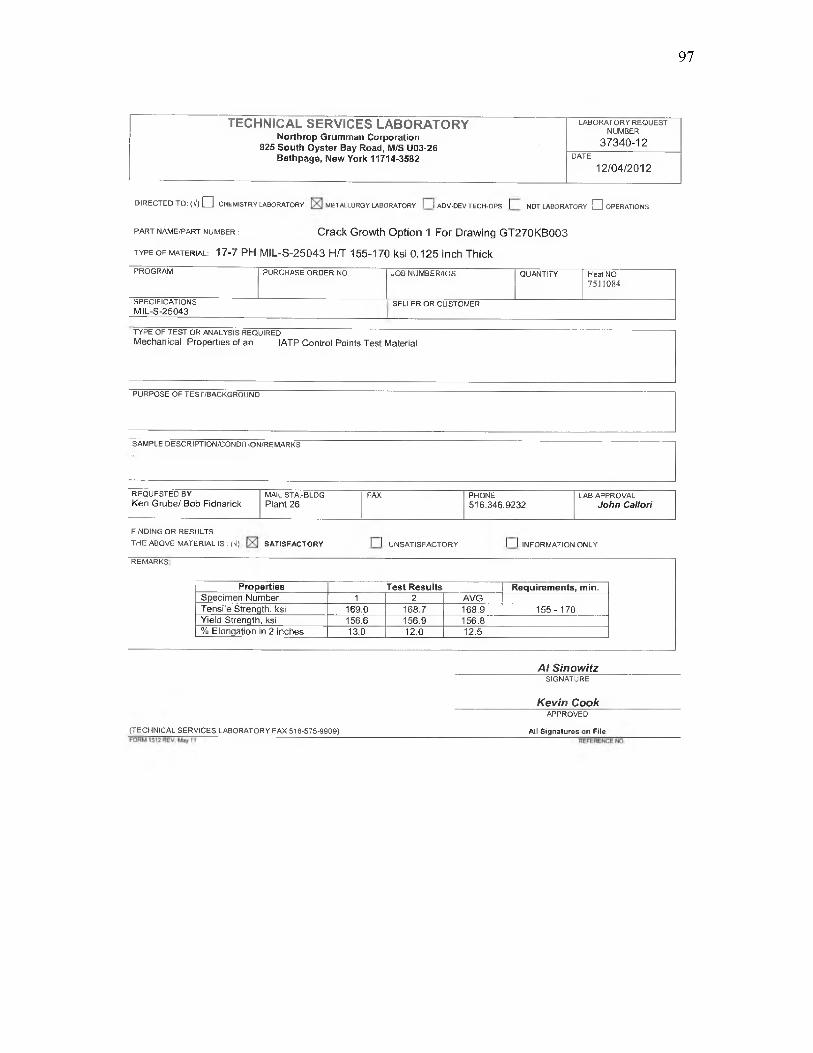
97
TECHNICAL SERVICES LABORATORYNorthrop Grumman Corporation
925 South Oyster Bay Road, M/S U03-26 Bethpage, New York 11714-3582
DIRECTED TO: { V ) 0 CHEMISTRY LABORATORY METALLURGY LABORATORY I ! ADV-DEV TECH-OPS I I NOT LABORATORY C H OPERATIONS
p a r t n a m e /p a r t n u m b e r : Crack Growth Option 1 For Drawing GT270KB003
t y p e o f m a t e r ia l : 17-7 PH MIL-S-25043 H/T 155-170 ksi 0.125 inch ThickPROGRAM PURCHASE ORDER NO. JOS NUMBER/IOS QUANTITY Heat NO.
7511084
SPECIFICATIONS SELLER OR CUSTOMERMIL-S-25043
TYPE OF TEST OR ANALYSIS REQUIREDMechanical Properties of an IATP Control Points Test Material
PURPOSE OF TEST/BACKGROUND
SAMPLE DESCRIPTION/CONDITtON/REMARKS
REQUESTED BYKen Grube/ Bob Fidnarick
MAIL STA.-BLDG Plant 26
FAX PHONE516.346.9232
LAB APPROVALJohn Callori
FINDING OR RESULTS THE ABOVE MATERIAL IS : (V) SA TISFA CTO RY 1 1 UNSATISFACTORY I I INFORMATION ONLY
REMARKS
Properties Test Results Requirements, min.Specimen Number 1 2 AVGTensile Strength, ksi 169.0 168.7 168.9 155 - 170Yield Strenqth, ksi 156.6 156.9 156.8% Elongation in 2 inches 13.0 12.0 12.5
_____ Al Sinowitz" SIGNATURE
Kevin CookAPPROVED
(TECHNICAL SERVICES LABORATORY FAX 516-575-9S09) All Signalures on File
LABORATORY REQUEST NUMBER
37340-12DATE
12/04/2012
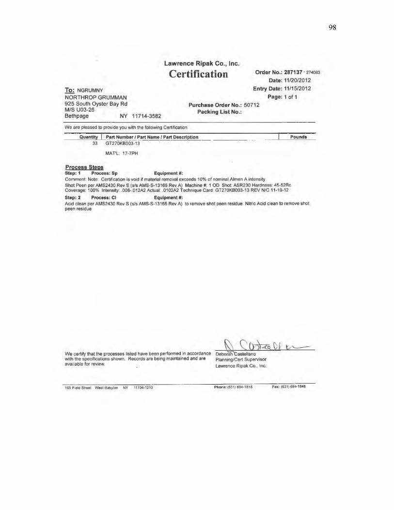
98

AA/\ WESTERN PROFESSIONAL, INC. 3460 BRADY CT. NE SALEM, OR 97301
PHONE (503)585-6263 FAX (503)585-6577w s m t u i \J\J\J
WWW. WESTPHOUB. DOM
www.westprolab.com
ULTRASONICS / PHASED ARRAY/EDM RESEARCH & DEVELOPEMENT
CUSTOMER: NORTHRUP GRUMMAN IT
P.O. 7500109433
S/N: PLATES 1 THRU 33
SIZE: 16" X 4" X , 125"
HEAT #: UNKNOWN
MATERIAL: 17-7 PH
DWG#: GT270KB003 DATE: 11-30-12
PLATE# DEPTH LENGTH WIDTH TYPE18 .0253” .0374" .0041” CORNER NOTCH19 .0206” .0305” .0037” CORNER NOTCH20 .0200” .0298” .0037” CORNER NOTCH21 .0209” .0308” .0038” CORNER NOTCH22 .0209” .0293” .0038” CORNER NOTCH23 .0207” .0328” .0039” CORNER NOTCH24 .0222” .0347" .0036” CORNER NOTCH25 .0213” .0313” .0041” CORNER NOTCH26 .0211” .0316” .0039” CORNER NOTCH27 .0205” .0308" .0039" CORNER NOTCH28 .0206" .0313” .0038" CORNER NOTCH29 .0202” .0313” .0037” CORNER NOTCH30 .0208” .0311” .0043” CORNER NOTCH31 .0219” .0330" .0041” CORNER NOTCH32 .0203” .0290” .0043” CORNER NOTCH33 .0217” .0333" .0043” CORNER NOTCH
PLATE# DEPTH LENGTH WIDTH TYPE1 .0201” .0297” .0044” CORNER NOTCH2 .0209” .0317” .0043” CORNER NOTCH
*3 .0217” .0313” .0040" CORNER NOTCH4 .0217” .0342” .0041” CORNER NOTCH5 .0201” .0307" ,0044” CORNER NOTCH6 .0202” .0285” .0044” CORNER NOTCH7 .0206” .0304” .0041" CORNER NOTCH8 .0215” .0303" .0041” CORNER NOTCH9 .0202” .0295” .0043” CORNER NOTCH10 .0215" .0314” .0043" CORNER NOTCH11 .0209" .0296” .0039” CORNER NOTCH12 .0208” .0309” .0039” CORNER NOTCH13 .0205" .0304" .0040” CORNER NOTCH14 .0209” .0321" .0039” CORNER NOTCH15 .0224" .0331” .0041” CORNER NOTCH16 ,0220” .0331” .0041" CORNER NOTCH17 .0206” .0304” .0037" CORNER NOTCH
* SEE ATTACHED NOTE
NOTE: SEE ATTACHED CUSTOMER DRAWING FOR NOTCH REQUIREMENTS AND LOCATION.
ALL DIMENSIONS ARE MEASURED WITH DIMENSIONAL EQUIPMENT WHICH IS FABRICATED BY: S. CHAMBERLAINCERTIFIED AND TRACEABLE TO NIST (#708) #5084918 AND NIST (#783183)#5830553. NUCLEAR REGULATORY COMMISSION RULES AND REGULATIONS 10CFR PART 21 APPLIES TO THIS ORDER, ALL NOTCHES MANUFACTURED PER APPROVED BYWESTPRO PROCEDURE WQC-IV.
NORTHRUP GRUMMAN IT PO# 7500109433 TEST SPECIMENS PAGE 1 OF 1
'O
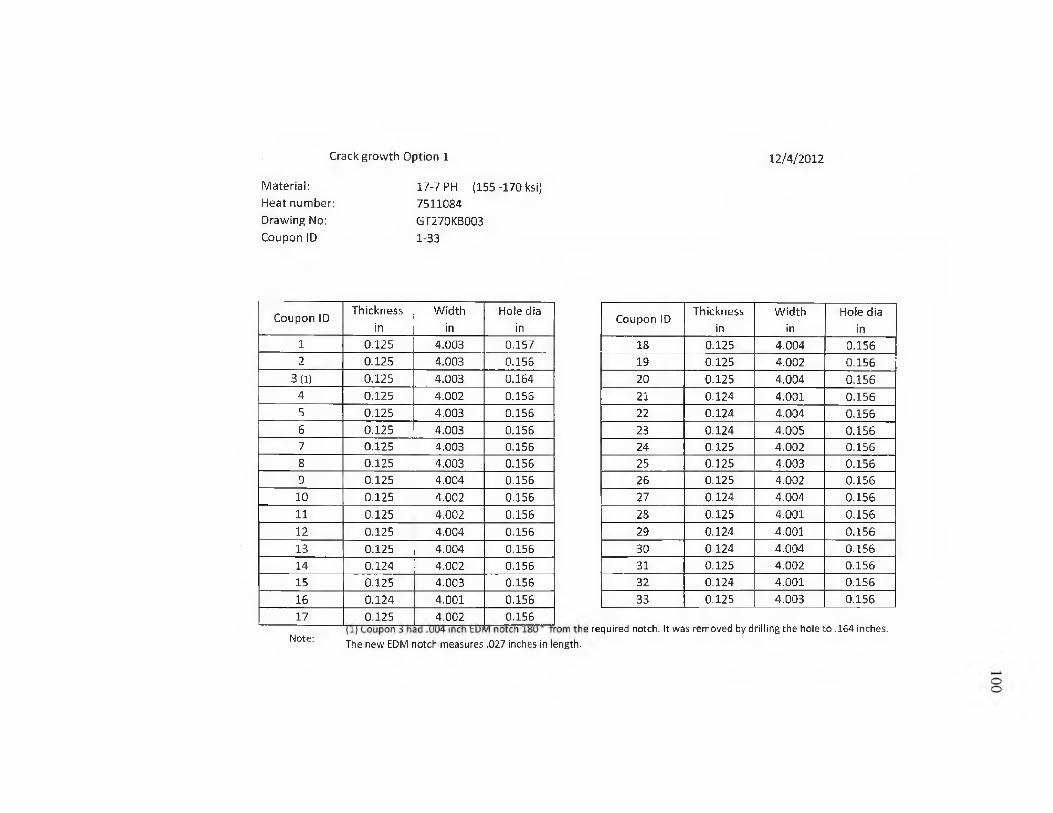
Crack growth Option 1 12/4/2012
Material: 17-7 PH (155-170 ksi)Heat number: 7511084Drawing No: GT270KB003Coupon ID 1-33
Coupon IDThickness
inWidth
inHole dia
in1 0.125 4.003 0.1572 0.125 4.003 0.156
3(1) 0.125 4.003 0.1644 0.125 4.002 0.1565 0.125 4.003 0.1566 0.125 4,003 0.1567 0.125 4,003 0.156S 0.125 4,003 0.1569 0.125 4.004 0.15610 0.125 4.002 0.15611 0.125 4.002 0.15612 0.125 4.004 0.15613 0.125 4.004 0.15614 0.124 4.002 0.15615 0.125 4.003 0.15616 0.124 4.001 0.15617 0.125 4.002 0.156
Coupon IDThickness
inWidth
inHole dia
in18 0.125 4.004 0.15619 0.125 4.002 0.15620 0.125 4.004 0.15621 0.124 4.001 0.15622 0.124 4.004 0,15623 0.124 4.005 0.15624 0.125 4.002 0.15625 0.125 4.003 0.15626 0.125 4.002 0.15627 0.124 4.004 0.15628 0.125 4.001 0.15629 0.124 4.001 0.15630 0.124 4.004 0.15631 0.125 4.002 0.15632 0.124 4.001 0.15633 0.125 4.003 0.156
Note:? required notch. It was removed by drilling the hole to .164 inches.
The new EDM notch measures .027 inches in length.

APPENDIX B
POLISHING, REAMING AND SEM PROCEDURES

102
PROCEDURE FOR POLISHING SURFACE OF TEST SPECIMENS
1. A progression of 500, 800 and 1200 grit sandpaper was used to remove the mill finish.
2. A Struers Tanspol-2 polisher was then used with a progression of polishing paste of 3 micron and 1 micron to polish the surface from the 1200 grit sand paper.
PROCEDURE FOR REAMING THE BORE OF THE TEST SPECIMENS
1. Find the center of the hole using a hole dial indicator mounted in the spindle of the mill.
2. Using a 15/64” drill bit, drill out the bore starting on the opposite side of where the precrack is located. This will help prevent the bit from catching on the crack. [26] The spindle, in high gear, was set at a speed of 700 rpm.
3. Using a 12 straight flute 0.25” reamer, slowly ream out the bore also starting on the side opposite the precrack. The spindle, in low gear, was set at 80 rpm.
PROCEDURE FOR POLISHING THE BORE OF THE TEST SPECIMENS
1. Use a 84922 silicon carbide sanding stone to remove reaming marks
2. Use a 462 rubber polishing cone point to remove the defects created by the sanding stone.
3. Apply 3 micron polishing paste to a polishing cloth wrapped around a 402 rotary tool mandrel.
PROCEDURE FOR USING THE SEM
1. Turn on the chiller to the SEM and wait for it to reach a temperature of 68°F.
2. Turn on power to the SEM.
3. Place the specimen in the vibrating cleaner containing a lacquer solution for 10 minutes.
4. Replace the lacquer solution with one of alcohol for another 10 minutes.
5. Release the vacuum from the observation chamber.
6. Using rubber gloves, place the cleaned specimen into the holding mount, close the chamber and turn on the vacuum pump.

103
7. Once the vacuum indicator signals that conditions are sufficient, the electron beam is turned on.
8. Adjust the focus, contrast and brightness until the image is clear. Initially keep a working distance of 15 to 20 mm to obtain a wide view of the surface.
9. Pick a desired location on the surface and magnify the image to 3,000X to 4,000X and focus the image. This will help produce higher quality pictures at smaller magnifications.
10. Once the image is focused, zoom back out to obtain the widest view desired.
11. Progressively take pictures by incrementally increasing the magnification until the desired amount of detail is obtained.
12. Once the examinations are complete, turn off the electron beam and the pump to release the vacuum from the observation chamber.
13. Using rubber gloves, open the observation chamber and remove the specimen.
14. Close the observation chamber and turn on the pump once more. This will help prevent contaminants from entering the chamber.
15. Once the observation chamber has sufficient vacuum applied, the power may then be turned off to both the SEM and chiller.

APPENDIX C
SOUTHWEST RESEARCH INSTITUTE EQUIPMENT
INFORMATION
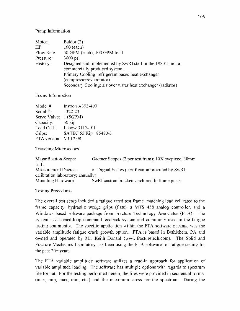
105
Pump Information
Motor: Baldor (2)HP: 100 (each)Flow Rate: 50 GPM (each), 100 GPM total Pressure: 3000 psiHistory: Designed and implemented by SwRI staff in the 1980’s; not a
commercially produced system.Primary Cooling: refrigerant based heat exchanger (compressor/evaporator).Secondary Cooling: air over water heat exchanger (radiator)
Frame Information
Model #: Serial #: Servo Valve: Capacity: Load Cell: Grips:
Instron A393-499 1322-231 (5GPM)50 kipLebow 3117-101 SATEC 55 Kip 185480-3
FTA version: V3.12.08
Traveling Microscopes
Magnification Scope: Gaetner Scopes (2 per test fram); 10X eyepiece, 38mmEFLMeasurement Device: 6” Digital Scales (certification provided by SwRIcalibration laboratory; annually)Mounting Hardware: SwRI custom brackets anchored to frame posts
Testing Procedures
The overall test setup included a fatigue rated test frame, matching load cell rated to the frame capacity, hydraulic wedge grips (flats), a MTS 458 analog controller, and a Windows based software package from Fracture Technology Associates (FTA). The system is a closed-loop command-feedback system and commonly used in the fatigue testing community. The specific application within the FTA software package was the variable amplitude fatigue crack growth option. FTA is based in Bethlehem, PA and owned and operated by Mr. Keith Donald (www.fracturetech.com). The Solid and Fracture Mechanics Laboratory has been using the FTA software for fatigue testing for the past 20+ years.
The FTA variable amplitude software utilizes a read-in approach for application of variable amplitude loading. The software has multiple options with regards to spectrum file format. For the testing performed herein, the files were provided in sequential format (max, min, max, min, etc.) and the maximum stress for the spectrum. During the

106
software read-in, it is determined whether or not the spectrum is an acceptable form and a simple summary of the spectrum is provided (number of points, maximum value within the spectrum, etc). During the test setup, the maximum load corresponding to the maximum stress is inputted and from there all of the spectrum file endpoints are scaled accordingly.
The FTA software is adaptive and learns during the first spectrum pass. A matrix is established for the particular spectrum content and loading parameters for the current test. The matrix contains information regarding the command signal needed for the multitude of loading segments within the spectrum file. During the first pass of the spectrum the matrix is populated with parameters associated with the command parameters and are used during subsequent passes as the test progress. In addition, the matrix is updated as specimen compliance changes thus requiring command parameter changes.
The backbone of variable amplitude testing is how well the system can achieve the target load level during each cycle; for spectra that have rather aggressive and deviating content, this becomes extremely important. The FTA system monitors the target and feedback values during the course of a test as a way to monitor and assess the performance. An absolute voltage level is entered as a parameter into the system as an acceptable threshold. Any difference between the target and feedback that is greater than this value and the event is archived in a file correlate to that test. It is important to note that this approach is an absolute difference (voltage) and not a relative difference (%). During the setup of a test and establishing the control parameters, the threshold value can be set to 0 volts such that every event is logged and can be post-test assessed to establish a history of error for a multiple spectrum passes. Furthermore, this history can be the basis for whether or not the current parameters are acceptable in terms of system performance and the frame is able to maintain under a certain acceptable amount of target/feedback error.
The FTA software controls test rate by utilizing both load rate and frequency as controlling parameters. The overall rate is bounded by these two parameters by inputting upper limits for both in terms of volts/time (loading rate) and frequency (cyclic rate). The system operates within these two bounds and depending the current cyclic content of the spectrum, is typically governed by one or the other. For example, during extreme events in a spectrum, the frequency limit may not be achievable and thus the loading rate becomes the controlling parameter during application of those events. Similarly, during low excursion events in a spectrum, the system may be easily able to handle a higher loading rate but is bound by an upper limit frequency. As previously mentioned, these two rate parameters are established during pretest exercises and are dependent on: the test frame, the spectrum content, coupon material, coupon geometry, load frame compliance, and acceptable error between target and feedback. During the testing of the 17-7PH SS, the frame was evaluated based on the above considerations when establishing the loading
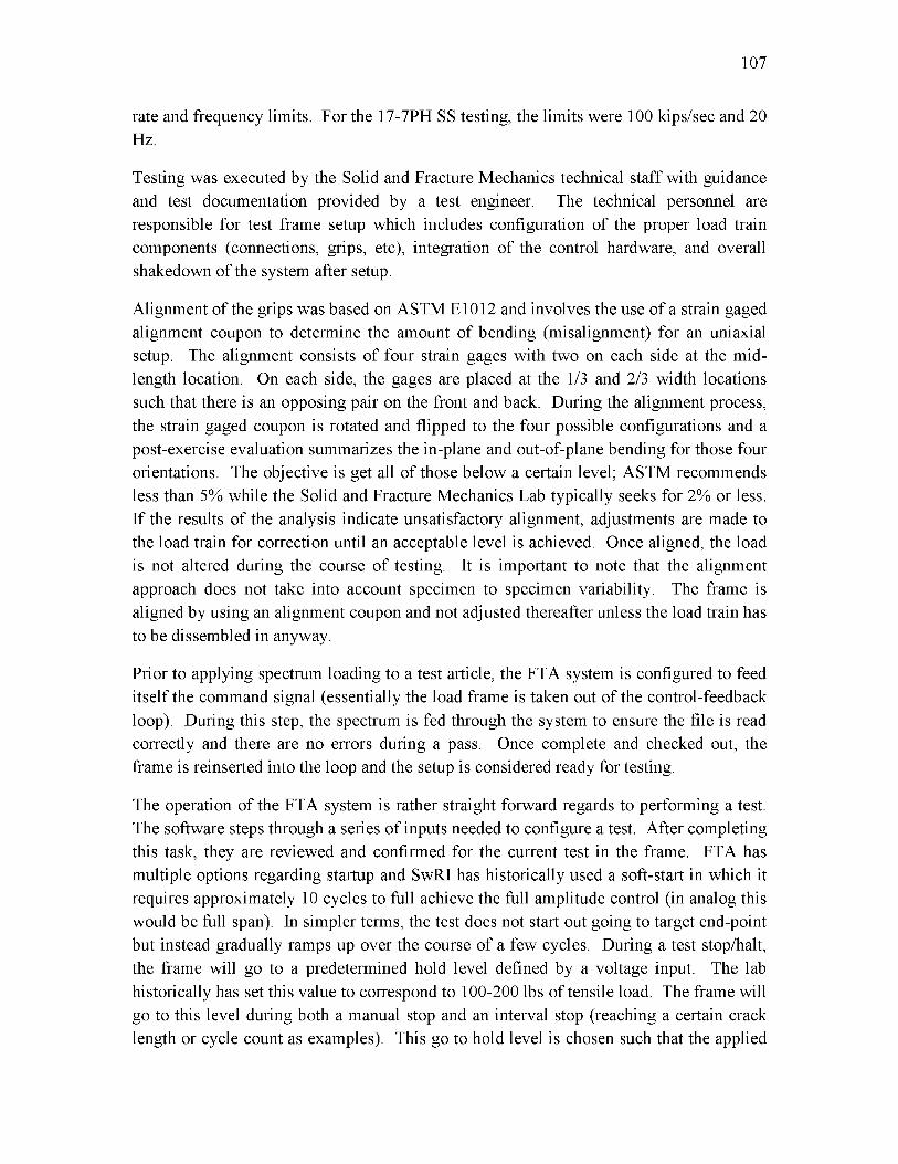
107
rate and frequency limits. For the 17-7PH SS testing, the limits were 100 kips/sec and 20 Hz.
Testing was executed by the Solid and Fracture Mechanics technical staff with guidance and test documentation provided by a test engineer. The technical personnel are responsible for test frame setup which includes configuration of the proper load train components (connections, grips, etc), integration of the control hardware, and overall shakedown of the system after setup.
Alignment of the grips was based on ASTM E1012 and involves the use of a strain gaged alignment coupon to determine the amount of bending (misalignment) for an uniaxial setup. The alignment consists of four strain gages with two on each side at the midlength location. On each side, the gages are placed at the 1/3 and 2/3 width locations such that there is an opposing pair on the front and back. During the alignment process, the strain gaged coupon is rotated and flipped to the four possible configurations and a post-exercise evaluation summarizes the in-plane and out-of-plane bending for those four orientations. The objective is get all of those below a certain level; ASTM recommends less than 5% while the Solid and Fracture Mechanics Lab typically seeks for 2% or less. If the results of the analysis indicate unsatisfactory alignment, adjustments are made to the load train for correction until an acceptable level is achieved. Once aligned, the load is not altered during the course o f testing. It is important to note that the alignment approach does not take into account specimen to specimen variability. The frame is aligned by using an alignment coupon and not adjusted thereafter unless the load train has to be dissembled in anyway.
Prior to applying spectrum loading to a test article, the FTA system is configured to feed itself the command signal (essentially the load frame is taken out of the control-feedback loop). During this step, the spectrum is fed through the system to ensure the file is read correctly and there are no errors during a pass. Once complete and checked out, the frame is reinserted into the loop and the setup is considered ready for testing.
The operation of the FTA system is rather straight forward regards to performing a test. The software steps through a series of inputs needed to configure a test. After completing this task, they are reviewed and confirmed for the current test in the frame. FTA has multiple options regarding startup and SwRI has historically used a soft-start in which it requires approximately 10 cycles to full achieve the full amplitude control (in analog this would be full span). In simpler terms, the test does not start out going to target end-point but instead gradually ramps up over the course of a few cycles. During a test stop/halt, the frame will go to a predetermined hold level defined by a voltage input. The lab historically has set this value to correspond to 100-200 lbs of tensile load. The frame will go to this level during both a manual stop and an interval stop (reaching a certain crack length or cycle count as examples). This go to hold level is chosen such that the applied
108
load during the hold has no potential to induce load history effects into the test history. During the course of these testing, technicians were responsible for crack length measurements which happened multiple times a day during the work week. During the weekends, on occasion there was a technician available to monitor the test and maintain cycling. However, during a non-active weekend, the specimen would hold at the input level until a technician addressed the frame.
Both surface (c) and bore (a) measurements were made during the test effort. Traveling microscopes were used to monitor and measure crack lengths. Surface measurements were rather straightforward with the scope and travel setup orthogonal and perpendicular to the face of the coupon. Bore measurements, however, were accomplished by angling the scope into the bore and making the required geometric corrections to account for the non-orthogonal measurement by the angled view.
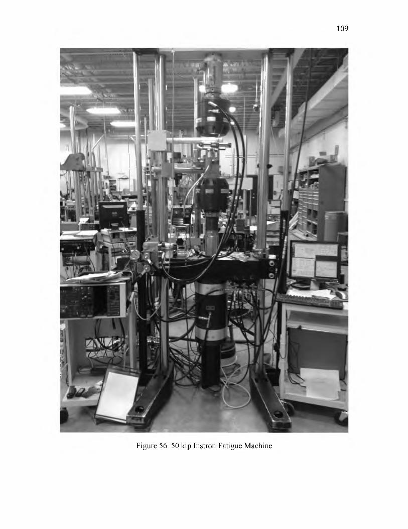
109
Figure 56 50 kip Instron Fatigue Machine
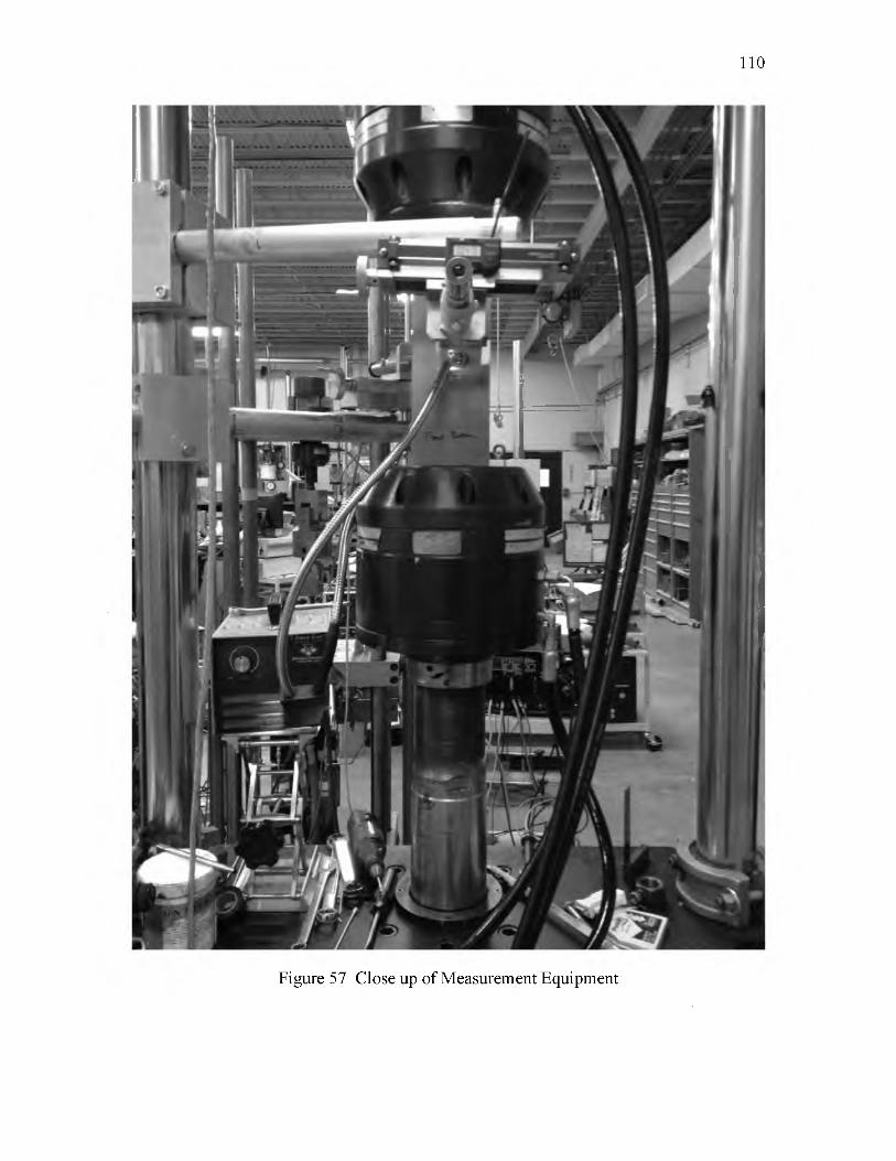
110
Figure 57 Close up of Measurement Equipment

APPENDIX D
FATIGUE MACHINE AND LOAD CELL CALIBRATION
CERTIFICATIONS
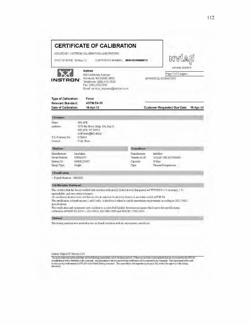
112
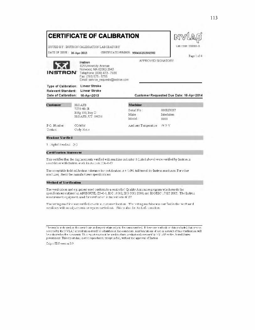
113
P.O. Number: CO 8616 Ambient Temperature : 79.3 °FC ontact: Cody Hone
Readout Verified
1. Digital Readout (in)
Certification Statement
This certifies that the displacements verified with machine indicator 1 (listed above) were verified by Instron in accordance with Instron work instruction ICA-8-G7.
The acceptable field calibration tolerance for certification is ± 1.0% full travel for Instron machines. For other machines, check the manufacturers specifications.
M ethod of Verification
The verification and equipment used conform to a controlled Quality Assurance program which meets the specifications outlined in ANSI/NCSL Z540-1, ISO 10012, ISO 9001:2008, andlSO/lEC 17025:2005. The Instron measurement equipment used for verification is traceable to NIST.
The testing machine was verified on-site at customer location. The testing machine was verified in the 'As Found1 condition with no adjustments or repairs carried out. This is also the 'As Left' condition.
The results indicated on this certificate and report relate only to the items venfied. If there are methods or data included that are not covered by the NVLAP accreditation it will be identified in the comments. Any limitations of use as a result of this verification will be indicated in the comments. This report must not be used to claim product endorsement by NVLAP or the United States government. This report shall not be reproduced, except in full, without the approval of Instron.
CalproSDS version 3.9
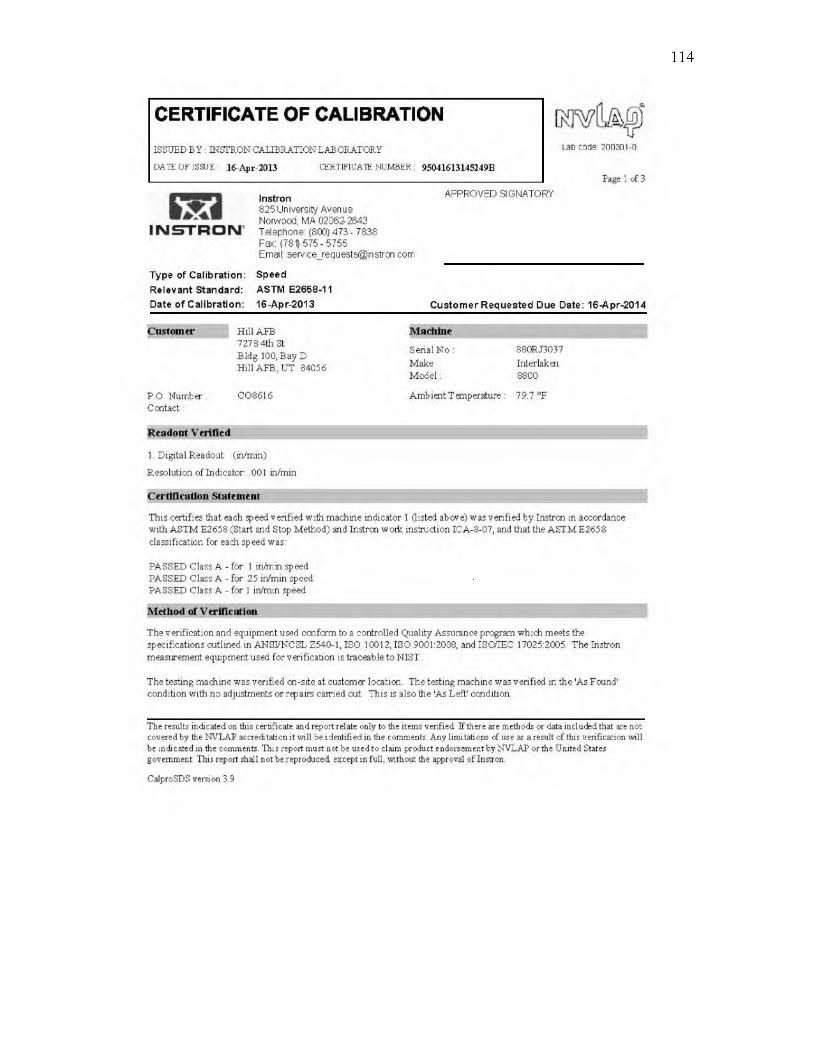
114

APPENDIX E
EXAMPLE OF PRECRACK CALCULATIONS

116
DIMENSIONS REQUIRED FOR CALCULATIONS
Crack Length in Hole (a) = 0.0510 in,Crack Length on Surface (c) = 0.0765 in,
Thickness (t)= 0.1250 in, Hole Diameter (d) = 0.1570 in, Hole Radius (r) = 0.0785 in,
Specimen Width (W) = 4.003 in, b = w/2 = 2.002 in
PRELIMINARY STEP CALCULATIONS
a/ c = 0.667, Q = 1 + 1.464 ( a/ c1'6S) = 1-750, a/ t = 0.408, r/ t = 0.628
CONSTANTS AND APPLIED STRESS
for tension loads ^ = 0.85, for single crack n = 1, S t = 15.4 ksi, bending correction factor Hch = 0 since there are no bending stresses
MAIN EQUATIONS FOR CALCULATING THE STRESS INTENSITY IN A SINGLECORNER CRACK OF A HOLE
1/4 a c \ j /4 ac\K°ne crack = + 2 f r ) / W + tr ) KtW0 CraCkS
^two cracks = (St + HchSb) J ^ F ch (~c , f , \ , \ , \ \ , $ )
for 0.2 < a/ c < 2, a/ t < 1,0.5 < r/ t < 2 ,(r + c )/^ < 0.5, and 0 < 0 < n / 2
Fch = Mi + M2 Q + M3 Q ] g 1g2gsg4f<pfw
for a/ c < 1 : M1 = 1.13 - 0 .09(a/ c), M2 = -0 .5 4 + 0 .89 /(0 .2 + a/ c),
M3 = 0.5 - 1 /(0 .6 5 + a/ c) + 14(1 - a/ c) 24,
g i = 1 + [0.1 + 0 .35(a/ t) 2] ( 1 - sin 0 )2,
1 + 0.3581 + 1.425A2 - 1.578A3 + 2.156A4 9 2 = 1 + 0.1322 ,

117
where A = 1 /(1 + c/r cos(u0)),
g 3 = (1 + 0 .0 4 a/ c)[1 + 0.1(1 - c o s 0 )2][O.85 + .15(a/ c) 1/4],
g 4 = 1 - 0 .7 (1 - a/ t ) (a /c - 0 .2)(1 - a /c) , = [(a /c)2 (cos0 )2 + (s in 0 )2] 1/4
/w = j sec @ secn ( 2 r + nc) a
4(6 — c) + 2nc^ t
1/2
These equations were input into an Excel spread to calculate the max stress intensities. Knowing the applied stress with the stress intensities the plastic zone sizes could then be calculated. The following is a printout of the spreadsheet used for the calculations.
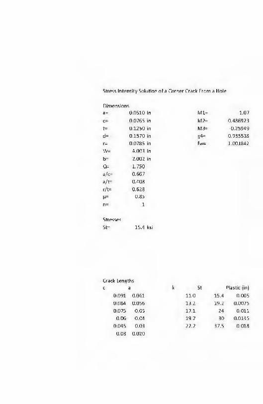
Stress Intensity Solution of a Corner Crack From a Hole
Dimensionsa= 0.0510 in Ml= 1,07
0.0765 in M2= 0.486923t= 0.1250 in M3= -0.25949d= 0.1570 in g4= 0.935538r= 0.0785 in fvj- 1.001842W= 4.003 inb= 2.002 inQ= 1.750a/c= 0.667a/t= 0.408r/t= 0.628H= 0.85n= 1
Stresses5t= 15.4 ksi
Crack Lengthsc a k St Plastic (in)
0.091 0.061 11.0 15.4 0.0050.084 0.056 13.2 19.2 0.00750.075 0.05 17,1 24 0.011
0.06 0.04 19.7 30 0.01450.045 0.03 22.2 37.5 0.018
0.03 0.020
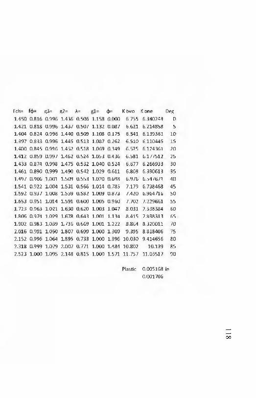
Fch= f<t>= Si= g2= A= 4>= K two K one Deg1.450 0.816 0.996 1.436 0.506 1.158 0.000 6.755 6.340244 01.421 0.818 0.996 1.437 0.507 1.132 0.087 6.621 6.214858 51.404 0.824 0.996 1.440 0.509 1.108 0.175 6.541 6.139361 101.397 0.833 0.996 1.445 0.513 1.087 0.262 6.510 6.110445 151.400 0.845 0.996 1.452 0.518 1.069 0.349 6.525 6.124361 201.412 0.859 0.997 1.462 0.524 1.053 0.436 6.581 6.177512 251.433 0.874 0.998 1.475 0.532 1.040 0.524 6.677 6.266933 301.461 0.890 0.999 1.490 0.542 1.029 0.611 6.808 6.390613 351.497 0.906 1.001 1.509 0.553 1,020 0.698 6.976 6.547671 401.541 0.922 1,004 1.531 0.566 1.014 0.785 7.179 6.738468 451.592 0.937 1.008 1.559 0.582 1.009 0.873 7.420 6.964716 501.653 0.951 1.014 1.591 0.600 1.005 0.960 7.702 7.229661 551.723 0.963 1.021 1.630 0.620 1.003 1.047 8.031 7.538384 601.806 0.974 1.029 1.678 0.643 1.001 1.134 8.415 7.898313 651.902 0.983 1.039 1.736 0.669 1,001 1,222 8.864 8.320011 702.016 0,991 1.050 1.807 0.699 1,000 1,309 9.395 8,818406 752.152 0.996 1.064 1.895 0.733 1.000 1,396 10.030 9.414656 802.318 0.999 1.079 2.007 0.771 1.000 1.484 10.802 10,139 852.523 1.000 1.095 2.148 0.815 1.000 1.571 11.757 11.03517 90
Plastic 0.005168 in 0.001706
118

APPENDIX F
PROCEDURES FOR AFGROW ANALYSIS

120
STEP BY STEP PROCESS TO USE AFGROW BASED ON THE GUIDELINES PREPARED BY THE UNITED STATES AIR FORCE [31]
1. Create Title: Brief description of model.
2. Select Material: This analysis used a file containing material properties and parameters for the Forman equation to simulate the 17-7PH in the AFGROW program. The information in the file is a general guide and some material properties may need to be adjusted based on manufacturing thicknesses or other factors. Reference the Metallic Materials Properties Development and Standardization (MMPDS) to verify correct material properties.
3. Create Model: From a selection of “Classic Models”, choose the appropriate geometric model. For this analysis, the “Single Corner Crack at Hole” model was chosen.a. Enter problem geometric factors including: thickness, width, hole diameter, initial
flaw size (IFS), offset, etc.i. Check: keep A/C constant
ii. Uncheck: Oblique through crackiii. IFS: Unless otherwise specified, the initial flaw size should be the same in
both the “A” and “C” directions. For this analysis an average of the precrack sizes, for each type of test conducted, were used.
b. Select Load Type: Ratio of tension or bearing stress to reference stress must be input for each load case (tension stress fraction = 1.0 if bearing stress is zero). The test for this analysis was purely tensile.
4. Open Spectrum File: For this analysis the A and B spectrum files, specifically created to be used in AFGROW, were utilized. AFGROW require that the files be normalized with the greatest value given a value of 1.0 and all other loads be represented as a fraction of the highest load.a. Stress Multiplication Factor (SMF): Enter the max stress of the spectrum. Since
the values in the spectrum files are representative of loads the SMF had to include a conversion factor to make the values in the spectrum files convert to stresses.
5. Select a Retardation Model: For this analysis several retardation models were attempted to obtain the best fit to the test data.
6. Predict Function Preferences: Used for establishing various analysis criteria and outputs.a. Select Growth Increments: Cycle by Cycle Beta and Spectrum calculation. Use a
Max Growth Increment of 0.25%b. Enter Output Intervals: Specify crack growth increments. Increment = 0.01”
i. Enter Number of Hours per Pass: Conversion factor for calculating effective flight hours (EFH) from segment count.
c. Select Output Options: Typically the user will select the data file and plot file options for crack growth data.

121
d. Select Propagation Limits: Unless otherwise specified use the Kmax and the Net Section Section Yield failure criteria.
i. If using Forman, as was done for this analysis, select User-Defined Kmax and enter an appropriate value for the material.
e. Enter Transition to Through Crack: Use default unless otherwise specified.
7. Select Stress State: Use default unless otherwise specified.
8. Select Beta Criteria: Use AFGROW standard solution betas for standard geometries.
9. At this point the user is ready to run the analysis.

APPENDIX G
CRACK GROWTH DATA SHEETS

123
GT270KB003-13-1 Fatigue Crack Growth Data SheetWidth: 4.003 in. Thick: 0.125 in. Area: 0.500 in
Pre-crack InformationPre-crack Date: 5/31/13 Hole Dia.: 0.156 in.
Loading Condition: Constant Amplitude R=0.05 Surface EDM: 0.0295 in.
Pre-crack Tuning DataTuning Step Frequency (Hz) Tuning Cycles Max Stress (ksi)
1 13 1057 37.52 13 420 303 15 550 244 20 1000 15.45 18 1279 15.4
Pre-crack Run DataCycles Stress (ksi) Frequency (Hz) Crack Length (in.)
0 0 0 0.10759800 37.5 13 0.1093
26564 37.5 13 0.111847564 30 13 0.121884580 24 15 0.1353118698 19.2 15 0.1407274222 15.4 18 0.1551
Experiment InformationExp. Date: SwRI 01/14 Loading Condition: Variable AmplitudeExp. Type: Spec. A & B1 Loading Rate: 100 kip/s Hole Dia.: 0.256 in.Max Stress (Sp. A&B): 21.953 ksi Surface Crack: 0.059 in. Bore Crack: 0.084 in.
Experiment Run Data
Spectrum EFHCrac k Length (in.)
CommentsFront Bore BackA 0 0.059 0.084
286.89 0.060 0.091B 0 0.060 0.091
137299.80 0.068 0.096274599.50 0.077 0.103411899.30 0.085 0.118456292.90 0.088 0.125 0.020503432.50 0.090 0.032549199.10 0.093 0.042
Continued on the next page
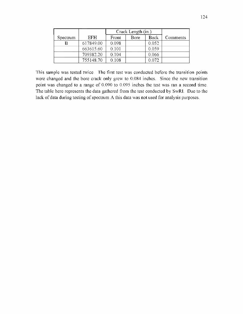
124
Spectrum EFHCrac k Length (in.)
CommentsFront Bore BackB 617849.00 0.098 0.052
663615.60 0.101 0.059709382.20 0.104 0.066755148.70 0.108 0.072
This sample was tested twice. The first test was conducted before the transition points were changed and the bore crack only grew to 0.084 inches. Since the new transition point was changed to a range of 0.090 to 0.095 inches the test was ran a second time. The table here represents the data gathered from the test conducted by SwRI. Due to the lack of data during testing of spectrum A this data was not used for analysis purposes.
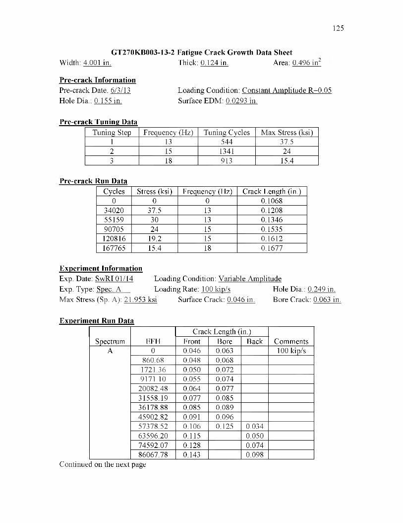
125
GT270KB003-13-2 Fatigue Crack Growth Data SheetWidth: 4.001 in. Thick: 0.124 in. Area: 0.496 in
Pre-crack InformationPre-crack Date: 6/3/13 Hole Dia.: 0.155 in.
Loading Condition: Constant Amplitude R=0.05 Surface EDM: 0.0293 in.
Pre-crack Tuning DataTuning Step Frequency (Hz) Tuning Cycles Max Stress (ksi)
1 13 544 37.52 15 1341 243 18 913 15.4
Pre-crack Run DataCycles Stress (ksi) Frequency (Hz) Crack Length (in.)
0 0 0 0.106834020 37.5 13 0.120855159 30 13 0.134690705 24 15 0.1535120816 19.2 15 0.1612167765 15.4 18 0.1677
Experiment InformationExp. Date: SwRI 01/14 Loading Condition: Variable AmplitudeExp. Type: Spec. A Loading Rate: 100 kip/s Hole Dia.: 0.249 in.Max Stress (Sp. A): 21.953 ksi Surface Crack: 0.046 in. Bore Crack: 0.063 in.
Experiment Run Data
Spectrum EFHCrac c Length (in.)
CommentsFront Bore BackA 0 0.046 0.063 100 kip/s
860.68 0.048 0.0681721.36 0.050 0.0729171.10 0.055 0.074
20082.48 0.064 0.07731558.19 0.077 0.08536178.88 0.085 0.08945902.82 0.091 0.09657378.52 0.106 0.125 0.03463596.20 0.115 0.05074592.07 0.128 0.07486067.78 0.143 0.098
Continued on the next page
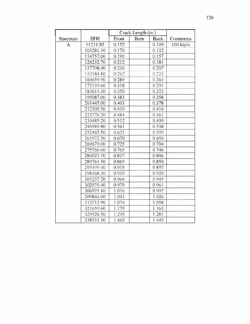
126
Crac k Length (in.)Spectrum EFH Front Bore Back Comments
A 91231.85 0.152 0.109 100 kip/s103281.30 0.170 0.132114757.00 0.190 0.157126232.70 0.212 0.181137708.40 0.236 0.207149184.10 0.262 0.233160659.90 0.289 0.263172135.60 0.318 0.291183611.30 0.350 0.323195087.00 0.383 0.358201445.00 0.403 0.378212300.50 0.439 0.416223776.20 0.484 0.461230485.20 0.512 0.490240989.80 0.561 0.538252465.50 0.621 0.599261072.30 0.670 0.650269679.00 0.725 0.704275766.60 0.765 0.746284023.70 0.827 0.806289761.50 0.869 0.850295499.40 0.915 0.897298368.30 0.939 0.920301237.20 0.964 0.945302970.40 0.979 0.961306975.10 1.016 0.997309844.00 1.043 1.026312712.90 1.074 1.058321659.60 1.179 1.163329926.50 1.295 1.281338533.30 1.460 1.449
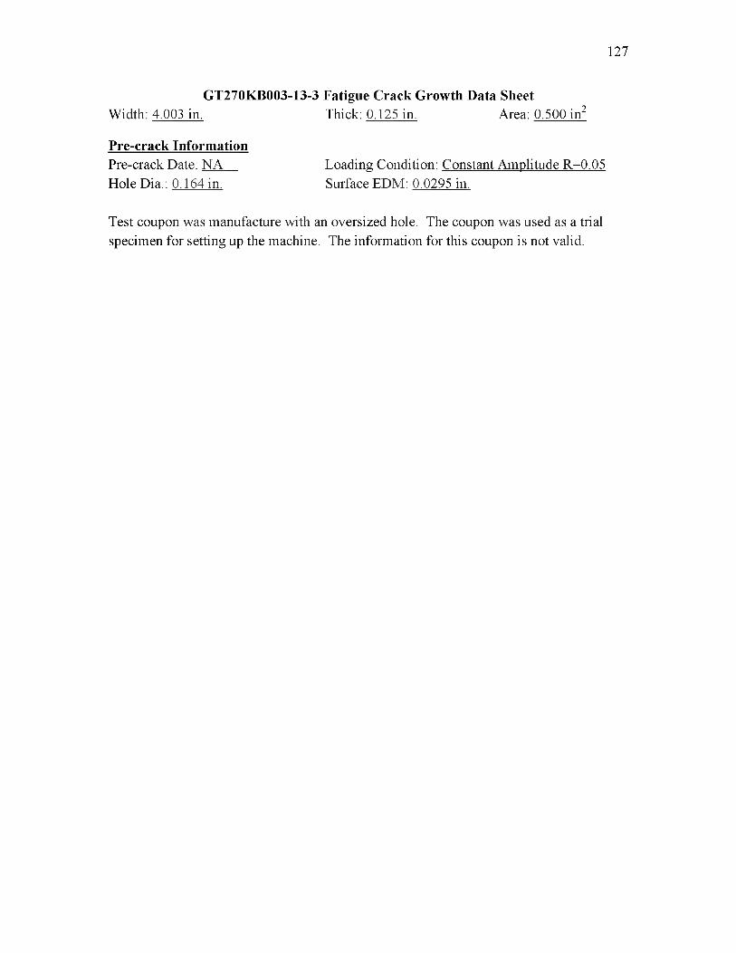
127
GT270KB003-13-3 Fatigue Crack Growth Data SheetWidth: 4.003 in. Thick: 0.125 in. Area: 0.500 in2
Pre-crack InformationPre-crack Date: NA Loading Condition: Constant Amplitude R=0.05Hole Dia.: 0.164 in. Surface EDM: 0.0295 in.
Test coupon was manufacture with an oversized hole. The coupon was used as a trial specimen for setting up the machine. The information for this coupon is not valid.
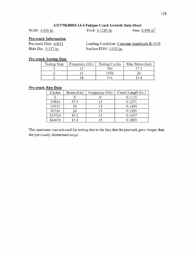
128
GT270KB003-13-4 Fatigue Crack Growth Data SheetWidth: 4.001 in. Thick: 0.1245 in. Area: 0.498 in2
Pre-crack InformationPre-crack Date: 6/4/13 Loading Condition: Constant Amplitude R=0.05Hole Dia.: 0.157 in. Surface EDM: 0.033 in.
Pre-crack Tuning DataTuning Step Frequency (Hz) Tuning Cycles Max Stress (ksi)
1 13 986 37.52 15 1556 243 18 NA 15.4
Pre-crack Run DataCycles Stress (ksi) Frequency (Hz) Crack Length (in.)
0 0 0 0.111533814 37.5 13 0.127153933 30 13 0.143090716 24 13 0.1565125924 19.2 15 0.1657164676 15.4 15 0.1803
This specimen was not used for testing due to the fact that the precrack grew longer than the previously determined range.
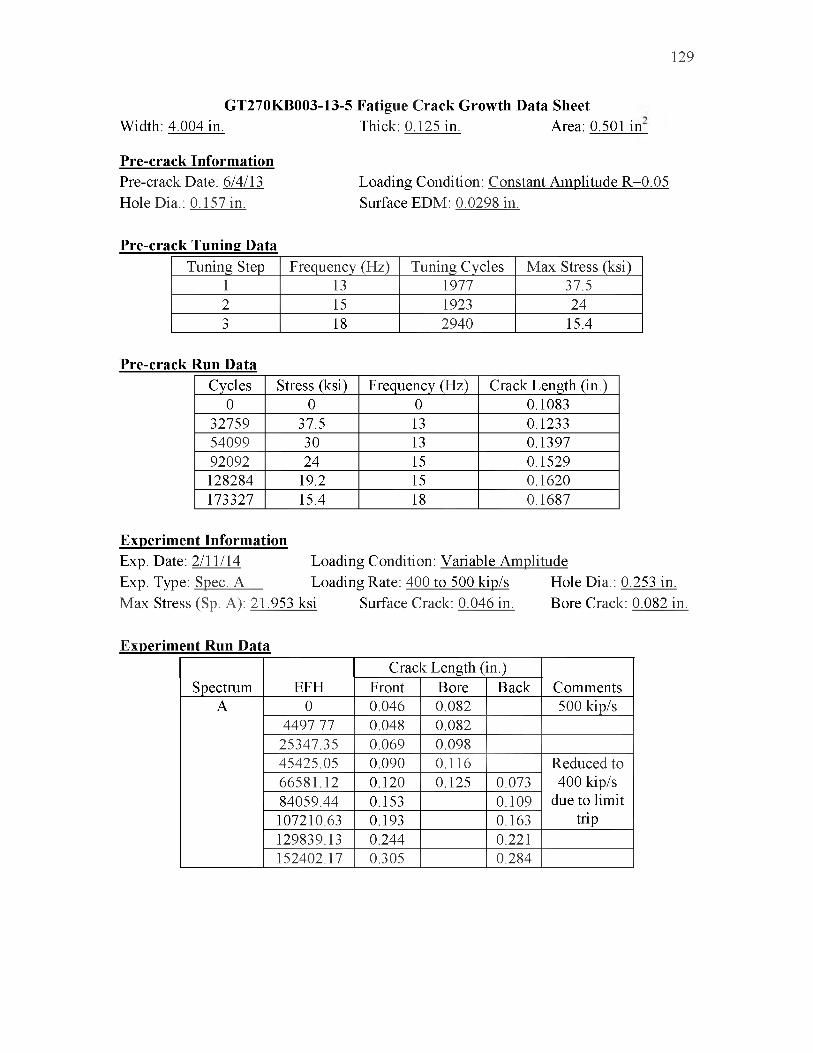
129
GT270KB003-13-5 Fatigue Crack Growth Data SheetWidth: 4.004 in. Thick: 0.125 in. Area: 0.501 in
Pre-crack InformationPre-crack Date: 6/4/13 Hole Dia.: 0.157 in.
Loading Condition: Constant Amplitude R=0.05 Surface EDM: 0.0298 in.
Pre-crack Tuning DataTuning Step Frequency (Hz) Tuning Cycles Max Stress (ksi)
1 13 1977 37.52 15 1923 243 18 2940 15.4
Pre-crack Run DataCycles Stress (ksi) Frequency (Hz) Crack Length (in.)
0 0 0 0.108332759 37.5 13 0.123354099 30 13 0.139792092 24 15 0.1529128284 19.2 15 0.1620173327 15.4 18 0.1687
Experiment InformationExp. Date: 2/11/14 Loading Condition: Variable AmplitudeExp. Type: Spec. A Loading Rate: 400 to 500 kip/s Hole Dia.: 0.253 in.Max Stress (Sp. A): 21.953 ksi Surface Crack: 0.046 in. Bore Crack: 0.082 in.
Experiment Run Data
Spectrum EFHCrac c Length (in.)
CommentsFront Bore BackA 0 0.046 0.082 500 kip/s
4497.77 0.048 0.08225347.35 0.069 0.09845425.05 0.090 0.116 Reduced to
400 kip/s due to limit
trip
66581.12 0.120 0.125 0.07384059.44 0.153 0.109107210.63 0.193 0.163129839.13 0.244 0.221152402.17 0.305 0.284

130
GT270KB003-13-6 Fatigue Crack Growth Data SheetWidth: 4.003 in. Thick: 0.125 in. Area: 0.500 in
Pre-crack InformationPre-crack Date: 6/5/13 Hole Dia.: 0.157 in.
Loading Condition: Constant Amplitude R=0.05 Surface EDM: 0.0298 in.
Pre-crack Tuning DataTuning Step Frequency (Hz) Tuning Cycles Max Stress (ksi)
1 13 1116 37.52 15 1722 243 18 2452 15.4
Pre-crack Run DataCycles Stress (ksi) Frequency (Hz) Crack Length (in.)
0 0 0 0.108330533 37.5 13 0.124149551 30 13 0.137582597 24 15 0.1521122787 19.2 15 0.1625168845 15.4 18 0.1681
Experiment InformationExp. Date: 9/6/13 Loading Condition: Variable AmplitudeExp. Type: Spec. A&B1 Loading Rate: 100 to 150kip/s Hole Dia.: 0.256 in.Max Stress (Sp. A&B): 21.953 ksi Surface Crack: 0.036 in. Bore Crack: 0.064 in.
Experiment Run Data
Spectrum EFHCrac c Length (in.)
CommentsFront Bore BackA 0 0.036 0.064 150 kip/s
5697.86 0.039 0.06911386.16 0.043 0.07017492.24 0.048 0.07326767.95 0.055 0.07835850.07 0.065 0.08837998.09 0.066 0.090
B 0 0.066 0.090 100 kip/s124387 0.068 0.093246174 0.071 0.094371934 0.073 0.097501119 0.073 0.099
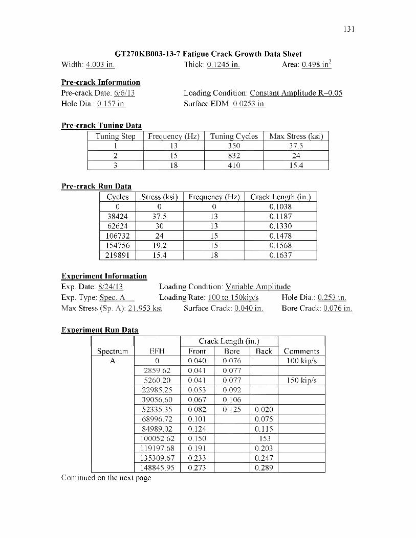
131
GT270KB003-13-7 Fatigue Crack Growth Data SheetWidth: 4.003 in. Thick: 0.1245 in. Area: 0.498 in2
Pre-crack InformationPre-crack Date: 6/6/13 Hole Dia.: 0.157 in.
Loading Condition: Constant Amplitude R=0.05 Surface EDM: 0.0253 in.
Pre-crack Tuning DataTuning Step Frequency (Hz) Tuning Cycles Max Stress (ksi)
1 13 350 37.52 15 832 243 18 410 15.4
Pre-crack Run DataCycles Stress (ksi) Frequency (Hz) Crack Length (in.)
0 0 0 0.103838424 37.5 13 0.118762624 30 13 0.1330106732 24 15 0.1478154756 19.2 15 0.1568219891 15.4 18 0.1637
Experiment InformationExp. Date: 8/24/13 Loading Condition: Variable AmplitudeExp. Type: Spec. A Loading Rate: 100 to 150kip/s Hole Dia.: 0.253 in.Max Stress (Sp. A): 21.953 ksi Surface Crack: 0.040 in. Bore Crack: 0.076 in.
Experiment Run DataCrack Length (in.)
Spectrum EFH Front Bore Back CommentsA 0 0.040 0.076 100 kip/s
2859.62 0.041 0.0775260.20 0.041 0.077 150 kip/s
22985.25 0.053 0.09239056.60 0.067 0.10652335.35 0.082 0.125 0.02068996.72 0.101 0.07584989.02 0.124 0.115100052.62 0.150 .153119197.68 0.191 0.203135309.67 0.233 0.247148845.95 0.273 0.289
Continued on the next page
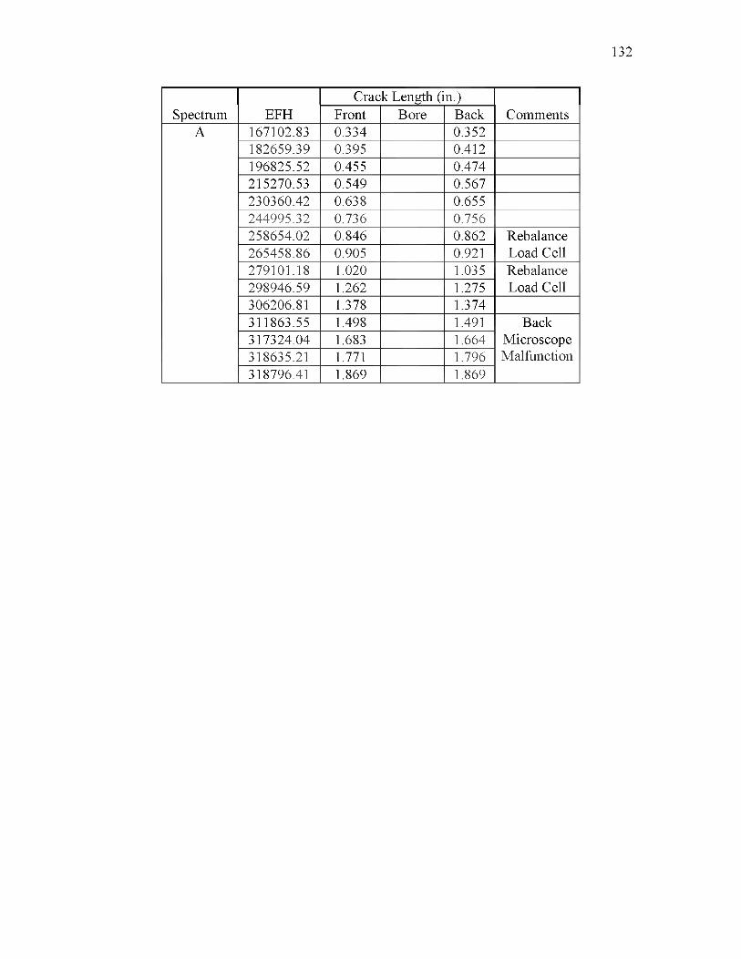
132
Crack Length (in.)Spectrum EFH Front Bore Back Comments
A 167102.83 0.334 0.352182659.39 0.395 0.412196825.52 0.455 0.474215270.53 0.549 0.567230360.42 0.638 0.655244995.32 0.736 0.756258654.02 0.846 0.862 Rebalance265458.86 0.905 0.921 Load Cell279101.18 1.020 1.035 Rebalance298946.59 1.262 1.275 Load Cell306206.81 1.378 1.374311863.55 1.498 1.491 Back317324.04 1.683 1.664 Microscope318635.21 1.771 1.796 Malfunction318796.41 1.869 1.869
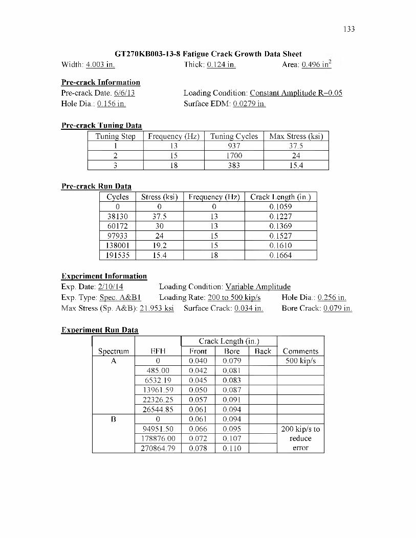
133
GT270KB003-13-8 Fatigue Crack Growth Data SheetWidth: 4.003 in. Thick: 0.124 in. Area: 0.496 in
Pre-crack InformationPre-crack Date: 6/6/13 Hole Dia.: 0.156 in.
Loading Condition: Constant Amplitude R=0.05 Surface EDM: 0.0279 in.
Pre-crack Tuning DataTuning Step Frequency (Hz) Tuning Cycles Max Stress (ksi)
1 13 937 37.52 15 1700 243 18 383 15.4
Pre-crack Run DataCycles Stress (ksi) Frequency (Hz) Crack Length (in.)
0 0 0 0.105938130 37.5 13 0.122760172 30 13 0.136997933 24 15 0.1527138001 19.2 15 0.1610191535 15.4 18 0.1664
Experiment InformationExp. Date: 2/10/14 Loading Condition: Variable AmplitudeExp. Type: Spec. A&B1 Loading Rate: 200 to 500 kip/s Hole Dia.: 0.256 in.Max Stress (Sp. A&B): 21.953 ksi Surface Crack: 0.034 in. Bore Crack: 0.079 in.
Experiment Run Data
Spectrum EFHCrac c Length (in.)
CommentsFront Bore BackA 0 0.040 0.079 500 kip/s
485.00 0.042 0.0816532.19 0.045 0.08313961.59 0.050 0.08722326.25 0.057 0.09126544.85 0.061 0.094
B 0 0.061 0.09494951.50 0.066 0.095 200 kip/s to
reduce error
178876.00 0.072 0.107270864.79 0.078 0.110

134
GT270KB003-13-9 Fatigue Crack Growth Data SheetWidth: 4.004 in. Thick: 0.1245 in. Area: 0.498 in
Pre-crack InformationPre-crack Date: 6/11/13 Hole Dia.: 0.157 in.
Loading Condition: Constant Amplitude R=0.05 Surface EDM: 0.0275 in.
Pre-crack Tuning DataTuning Step Frequency (Hz) Tuning Cycles Max Stress (ksi)
1 13 688 37.52 15 1924 243 18 223 15.4
Pre-crack Run DataCycles Stress (ksi) Frequency (Hz) Crack Length (in.)
0 0 0 0.106034752 37.5 13 0.122257045 30 13 0.135994318 24 15 0.1507136224 19.2 15 0.1603201320 15.4 18 0.1679
Experiment InformationExp. Date: 9/14/13 Loading Condition: Variable AmplitudeExp. Type: Spec. A&B2 Loading Rate: 100 kip/s Hole Dia.: 0.255 in.Max Stress (Sp. A&B): 21.953 ksi Surface Crack: 0.041 in. Bore Crack: 0.069 in.
Experiment Run Data
Spectrum EFHCrac c Length (in.)
CommentsFront Bore BackA 0 0.040 0.069
16995.52 0.054 0.07929381.79 0.066 0.08738063.86 0.075 0.09645886.61 0.085 0.10547109.23 0.086 0.106
B 0 0.086 0.10637267.90 0.089 0.10963537.18 0.092 0.11392216.88 0.093 0.116112156.03 0.096 0.117
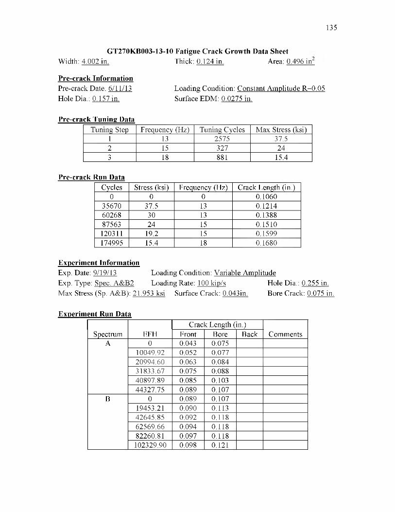
135
GT270KB003-13-10 Fatigue Crack Growth Data SheetWidth: 4.002 in. Thick: 0.124 in. Area: 0.496 in
Pre-crack InformationPre-crack Date: 6/11/13 Hole Dia.: 0.157 in.
Loading Condition: Constant Amplitude R=0.05 Surface EDM: 0.0275 in.
Pre-crack Tuning DataTuning Step Frequency (Hz) Tuning Cycles Max Stress (ksi)
1 13 2575 37.52 15 327 243 18 881 15.4
Pre-crack Run DataCycles Stress (ksi) Frequency (Hz) Crack Length (in.)
0 0 0 0.106035670 37.5 13 0.121460268 30 13 0.138887563 24 15 0.1510120311 19.2 15 0.1599174995 15.4 18 0.1680
Experiment InformationExp. Date: 9/19/13 Loading Condition: Variable AmplitudeExp. Type: Spec. A&B2 Loading Rate: 100 kip/s Hole Dia.: 0.255 in.Max Stress (Sp. A&B): 21.953 ksi Surface Crack: 0.043in. Bore Crack: 0.075 in.
Experiment Run Data
Spectrum EFHCrac c Length (in.)
CommentsFront Bore BackA 0 0.043 0.075
10049.92 0.052 0.07720994.60 0.063 0.08431833.67 0.075 0.08840897.89 0.085 0.10344327.75 0.089 0.107
B 0 0.089 0.10719453.21 0.090 0.11342645.85 0.092 0.11862569.66 0.094 0.11882260.81 0.097 0.118102329.90 0.098 0.121
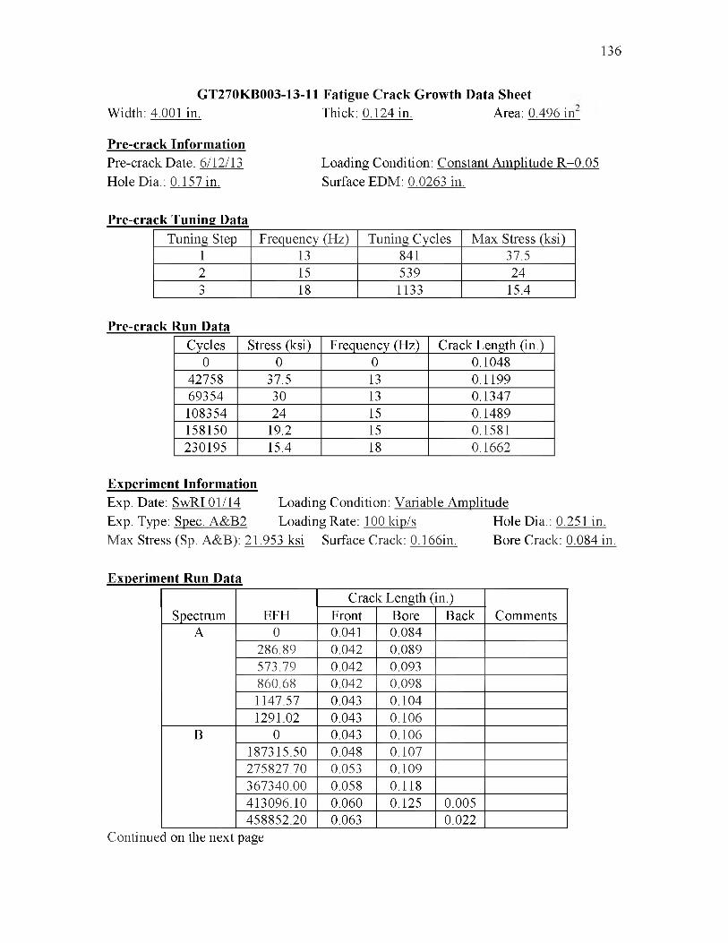
136
GT270KB003-13-11 Fatigue Crack Growth Data SheetWidth: 4.001 in. Thick: 0.124 in. Area: 0.496 in
Pre-crack InformationPre-crack Date: 6/12/13 Hole Dia.: 0.157 in.
Loading Condition: Constant Amplitude R=0.05 Surface EDM: 0.0263 in.
Pre-crack Tuning DataTuning Step Frequency (Hz) Tuning Cycles Max Stress (ksi)
1 13 841 37.52 15 539 243 18 1133 15.4
Pre-crack Run DataCycles Stress (ksi) Frequency (Hz) Crack Length (in.)
0 0 0 0.104842758 37.5 13 0.119969354 30 13 0.1347108354 24 15 0.1489158150 19.2 15 0.1581230195 15.4 18 0.1662
Experiment InformationExp. Date: SwRI 01/14 Loading Condition: Variable AmplitudeExp. Type: Spec. A&B2 Loading Rate: 100 kip/s Hole Dia.: 0.251 in.Max Stress (Sp. A&B): 21.953 ksi Surface Crack: 0.166in. Bore Crack: 0.084 in.
Experiment Run Data
Spectrum EFHCrac c Length (in.)
CommentsFront Bore BackA 0 0.041 0.084
286.89 0.042 0.089573.79 0.042 0.093860.68 0.042 0.0981147.57 0.043 0.1041291.02 0.043 0.106
B 0 0.043 0.106187315.50 0.048 0.107275827.70 0.053 0.109367340.00 0.058 0.118413096.10 0.060 0.125 0.005458852.20 0.063 0.022
Continued on the next page
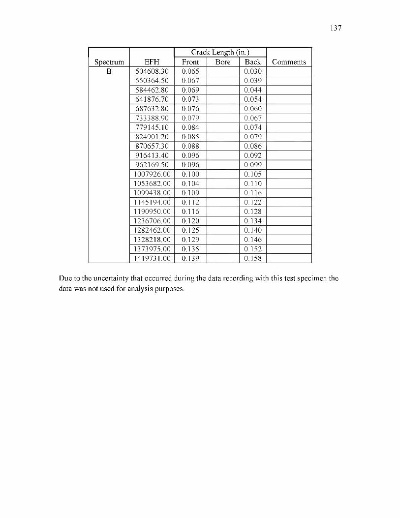
137
Crac k Length (in.)Spectrum EFH Front Bore Back Comments
B 504608.30 0.065 0.030550364.50 0.067 0.039584462.80 0.069 0.044641876.70 0.073 0.054687632.80 0.076 0.060733388.90 0.079 0.067779145.10 0.084 0.074824901.20 0.085 0.079870657.30 0.088 0.086916413.40 0.096 0.092962169.50 0.096 0.0991007926.00 0.100 0.1051053682.00 0.104 0.1101099438.00 0.109 0.1161145194.00 0.112 0.1221190950.00 0.116 0.1281236706.00 0.120 0.1341282462.00 0.125 0.1401328218.00 0.129 0.1461373975.00 0.135 0.1521419731.00 0.139 0.158
Due to the uncertainty that occurred during the data recording with this test specimen the data was not used for analysis purposes.

138
GT270KB003-13-12 Fatigue Crack Growth Data SheetWidth: 4.003 in. Thick: 0.125 in. Area: 0.500 in
Pre-crack InformationPre-crack Date: 6/14/13 Hole Dia.: 0.157 in.
Loading Condition: Constant Amplitude R=0.05 Surface EDM: 0.0263 in.
Pre-crack Tuning DataTuning Step Frequency (Hz) Tuning Cycles Max Stress (ksi)
1 13 1933 37.52 15 575 243 18 853 15.4
Pre-crack Run DataCycles Stress (ksi) Frequency (Hz) Crack Length (in.)
0 0 0 0.104833275 37.5 13 0.122853135 30 13 0.136380881 24 15 0.1494109655 19.2 15 0.1586154643 15.4 18 0.1644
Experiment InformationExp. Date: SwRI 01/14 Loading Condition: Variable AmplitudeExp. Type: Spec. A&B3 Loading Rate: 100 kip/s Hole Dia.: 0.253 in.Max Stress (Sp. A&B): 21.953 ksi Surface Crack: 0.043in. Bore Crack: 0.079 in.
Experiment Run Data
Spectrum EFHCrac c Length (in.)
CommentsFront Bore BackA 0 0.043 0.079
2868.93 0.043 0.0895737.85 0.047 0.09411475.70 0.048 0.09720082.48 0.057 0.10328689.26 0.065 0.10937296.04 0.075 0.125
B 0 0.075 0.12591512.24 0.083 0.012
217561.66 0.091 0.041411805.08 0.104 0.072594829.56 0.122 0.097
Continued onto next page
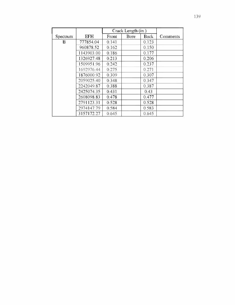
139
Crac k Length (in.)Spectrum EFH Front Bore Back Comments
B 777854.04 0.141 0.123960878.52 0.162 0.1501143903.00 0.186 0.1771326927.48 0.213 0.2061509951.96 0.242 0.2371692976.44 0.275 0.2711876000.92 0.309 0.3072059025.40 0.348 0.3472242049.87 0.388 0.3872425074.35 0.431 0.432608098.83 0.478 0.4772791123.31 0.528 0.5282974147.79 0.584 0.5833157172.27 0.645 0.645

140
GT270KB003-13-13 Fatigue Crack Growth Data SheetWidth: 4.003 in. Thick: 0.1245 in. Area: 0.498 in
Pre-crack InformationPre-crack Date: 6/17/13 Hole Dia.: 0.157 in.
Loading Condition: Constant Amplitude R=0.05 Surface EDM: 0.0275 in.
Pre-crack Tuning DataTuning Step Frequency (Hz) Tuning Cycles Max Stress (ksi)
1 13 1299 37.52 15 495 243 18 1686 15.4
Pre-crack Run DataCycles Stress (ksi) Frequency (Hz) Crack Length (in.)
0 0 0 0.106043161 37.5 13 0.123763551 30 13 0.1359100966 24 15 0.1513141206 19.2 15 0.1602197463 15.4 18 0.1671
Experiment InformationExp. Date: 2/17/14 Loading Condition: Variable AmplitudeExp. Type: Spec. A&B3 Loading Rate: 100 kip/s Hole Dia.: 0.252 in.Max Stress (Sp. A&B): 21.953 ksi Surface Crack: 0.042in. Bore Crack: 0.080 in.
Experiment Run Data
Spectrum EFHCrac c Length (in.)
CommentsFront Bore BackA 0 0.042 0.080
16794.60 0.055 0.09230331.40 0.065 0.09743958.80 0.078 0.11447717.70 0.083 0.124
B 0. 0.083 0.124 0.0034710.40 0.085 0.01659157.70 0.087 0.028123226.30 0.093 0.044169943.60 0.096 0.048
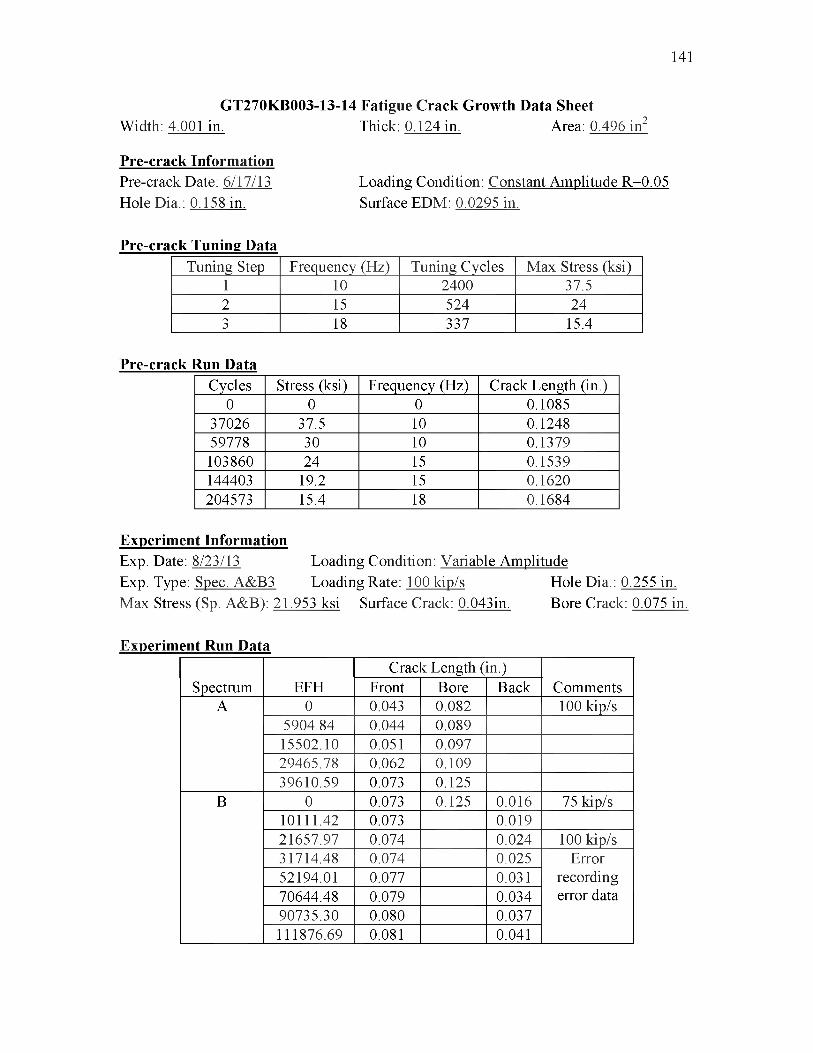
141
GT270KB003-13-14 Fatigue Crack Growth Data SheetWidth: 4.001 in. Thick: 0.124 in. Area: 0.496 in2
Pre-crack InformationPre-crack Date: 6/17/13 Hole Dia.: 0.158 in.
Loading Condition: Constant Amplitude R=0.05 Surface EDM: 0.0295 in.
Pre-crack Tuning DataTuning Step Frequency (Hz) Tuning Cycles Max Stress (ksi)
1 10 2400 37.52 15 524 243 18 337 15.4
Pre-crack Run DataCycles Stress (ksi) Frequency (Hz) Crack Length (in.)
0 0 0 0.108537026 37.5 10 0.124859778 30 10 0.1379103860 24 15 0.1539144403 19.2 15 0.1620204573 15.4 18 0.1684
Experiment InformationExp. Date: 8/23/13 Loading Condition: Variable AmplitudeExp. Type: Spec. A&B3 Loading Rate: 100 kip/s Hole Dia.: 0.255 in.Max Stress (Sp. A&B): 21.953 ksi Surface Crack: 0.043in. Bore Crack: 0.075 in.
Experiment Run Data
Spectrum EFHCrac c Length (in.)
CommentsFront Bore BackA 0 0.043 0.082 100 kip/s
5904.84 0.044 0.08915502.10 0.051 0.09729465.78 0.062 0.10939610.59 0.073 0.125
B 0 0.073 0.125 0.016 75 kip/s10111.42 0.073 0.01921657.97 0.074 0.024 100 kip/s31714.48 0.074 0.025 Error
recording error data
52194.01 0.077 0.03170644.48 0.079 0.03490735.30 0.080 0.037111876.69 0.081 0.041

GT270KB003-13-15 to 26 Fatigue Crack Growth Data Sheets
These test specimens were reserved for another test and are not included in this report.
142
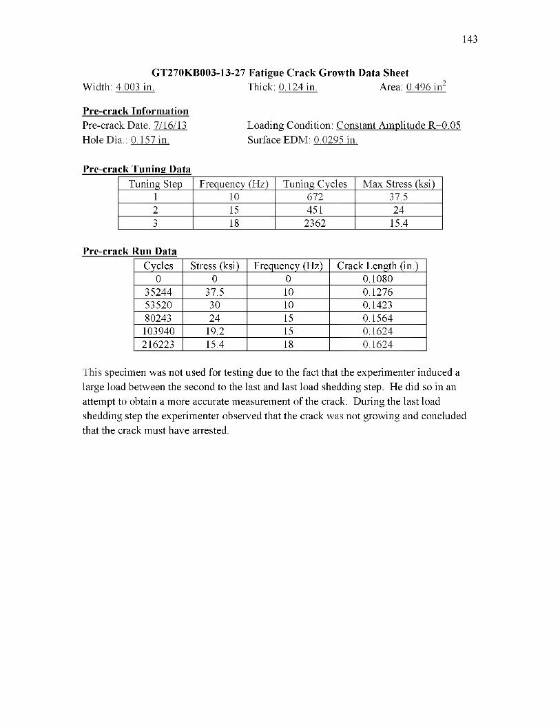
143
GT270KB003-13-27 Fatigue Crack Growth Data SheetWidth: 4.003 in. Thick: 0.124 in. Area: 0.496 in2
Pre-crack InformationPre-crack Date: 7/16/13 Loading Condition: Constant Amplitude R=0.05Hole Dia.: 0.157 in. Surface EDM: 0.0295 in.
Pre-crack Tuning DataTuning Step Frequency (Hz) Tuning Cycles Max Stress (ksi)
1 10 672 37.52 15 451 243 18 2362 15.4
Pre-crack Run DataCycles Stress (ksi) Frequency (Hz) Crack Length (in.)
0 0 0 0.108035244 37.5 10 0.127653520 30 10 0.142380243 24 15 0.1564103940 19.2 15 0.1624216223 15.4 18 0.1624
This specimen was not used for testing due to the fact that the experimenter induced a large load between the second to the last and last load shedding step. He did so in an attempt to obtain a more accurate measurement of the crack. During the last load shedding step the experimenter observed that the crack was not growing and concluded that the crack must have arrested.
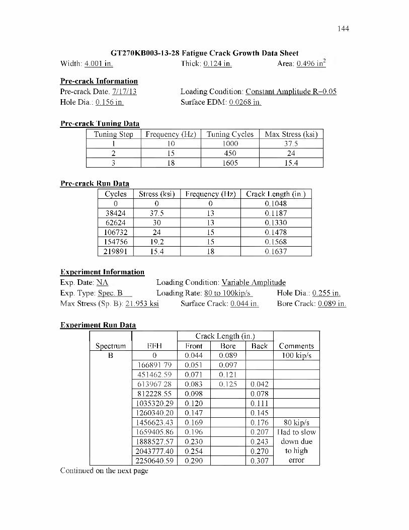
144
GT270KB003-13-28 Fatigue Crack Growth Data SheetWidth: 4.001 in. Thick: 0.124 in. Area: 0.496 in
Pre-crack InformationPre-crack Date: 7/17/13 Hole Dia.: 0.156 in.
Loading Condition: Constant Amplitude R=0.05 Surface EDM: 0.0268 in.
Pre-crack Tuning DataTuning Step Frequency (Hz) Tuning Cycles Max Stress (ksi)
1 10 1000 37.52 15 450 243 18 1605 15.4
Pre-crack Run DataCycles Stress (ksi) Frequency (Hz) Crack Length (in.)
0 0 0 0.104838424 37.5 13 0.118762624 30 13 0.1330106732 24 15 0.1478154756 19.2 15 0.1568219891 15.4 18 0.1637
Experiment InformationExp. Date: NA Loading Condition: Variable AmplitudeExp. Type: Spec. B Loading Rate: 80 to 100kip/s Hole Dia.: 0.255 in.Max Stress (Sp. B): 21.953 ksi Surface Crack: 0.044 in. Bore Crack: 0.089 in.
Experiment Run DataCrack Length (in.)
Spectrum EFH Front Bore Back CommentsB 0 0.044 0.089 100 kip/s
166891.79 0.051 0.097451462.59 0.071 0.121613967.28 0.083 0.125 0.042812228.55 0.098 0.0781035320.29 0.120 0.1111260340.20 0.147 0.1451456623.43 0.169 0.176 80 kip/s1659405.86 0.196 0.207 Had to slow1888527.57 0.230 0.243 down due2043777.40 0.254 0.270 to high2250640.59 0.290 0.307 error
Continued on the next page

145
Spectrum EFHCrack Length (in.)
CommentsFront Bore BackB 2366726.38 0.311 0.327
2504731.41 0.339 0.3562707055.36 0.382 0.4002755073.67 0.395 0.411
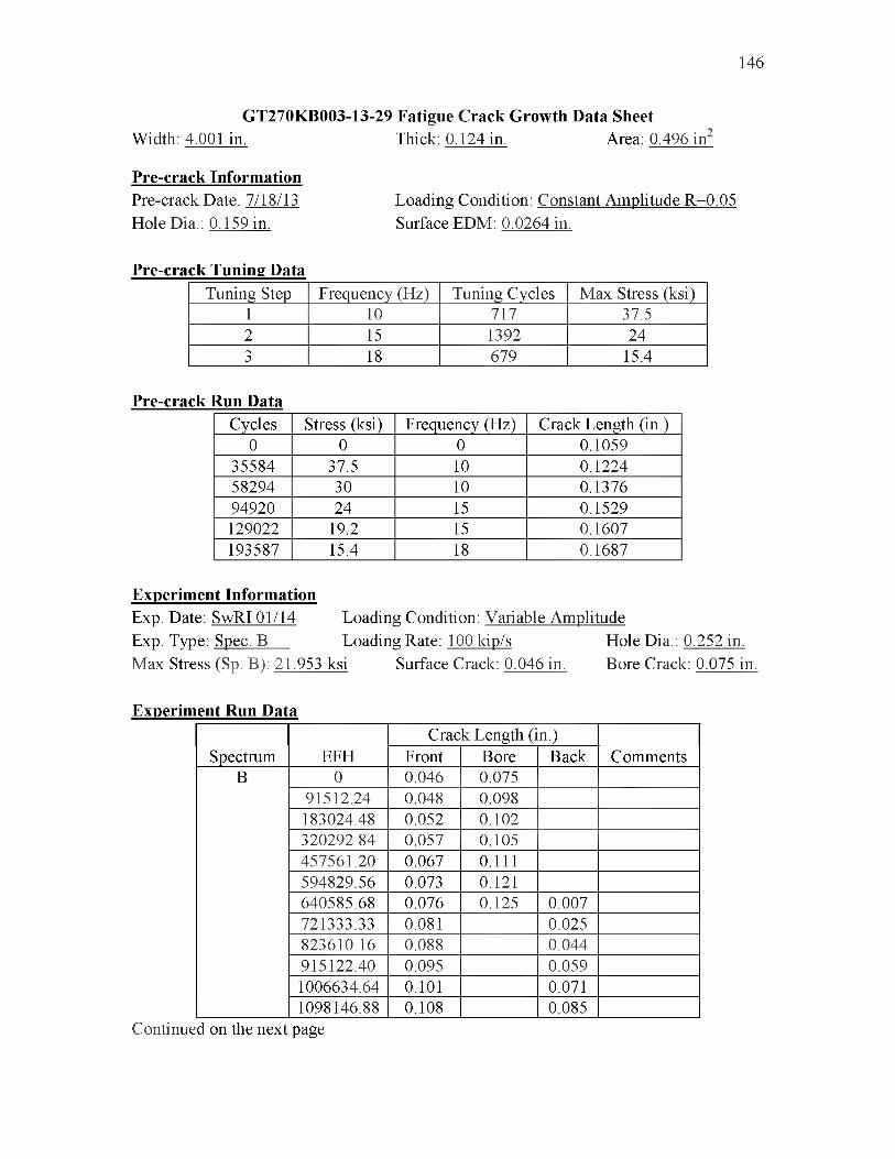
146
GT270KB003-13-29 Fatigue Crack Growth Data SheetWidth: 4.001 in. Thick: 0.124 in. Area: 0.496 in
Pre-crack InformationPre-crack Date: 7/18/13 Hole Dia.: 0.159 in.
Loading Condition: Constant Amplitude R=0.05 Surface EDM: 0.0264 in.
Pre-crack Tuning DataTuning Step Frequency (Hz) Tuning Cycles Max Stress (ksi)
1 10 717 37.52 15 1392 243 18 679 15.4
Pre-crack Run DataCycles Stress (ksi) Frequency (Hz) Crack Length (in.)
0 0 0 0.105935584 37.5 10 0.122458294 30 10 0.137694920 24 15 0.1529129022 19.2 15 0.1607193587 15.4 18 0.1687
Experiment InformationExp. Date: SwRI 01/14 Loading Condition: Variable AmplitudeExp. Type: Spec. B Loading Rate: 100 kip/s Hole Dia.: 0.252 in.Max Stress (Sp. B): 21.953 ksi Surface Crack: 0.046 in. Bore Crack: 0.075 in.
Experiment Run DataCrack Length (in.)
Spectrum EFH Front Bore Back CommentsB 0 0.046 0.075
91512.24 0.048 0.098183024.48 0.052 0.102320292.84 0.057 0.105457561.20 0.067 0.111594829.56 0.073 0.121640585.68 0.076 0.125 0.007721333.33 0.081 0.025823610.16 0.088 0.044915122.40 0.095 0.0591006634.64 0.101 0.0711098146.88 0.108 0.085
Continued on the next page

147
Spectrum EFHCrack Length (in.)
CommentsFront Bore BackB 1189659.12 0.117 0.098
1223881.49 0.120 0.103
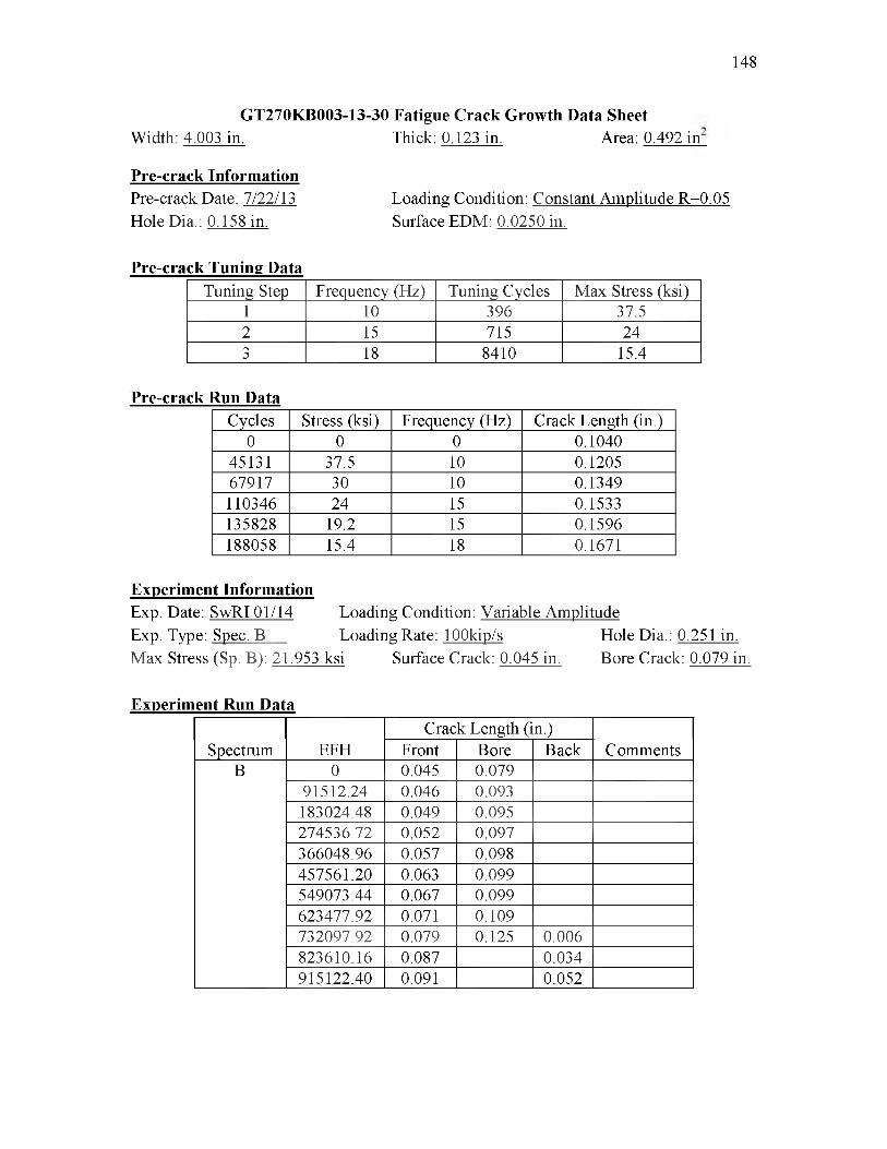
148
GT270KB003-13-30 Fatigue Crack Growth Data SheetWidth: 4.003 in. Thick: 0.123 in. Area: 0.492 in
Pre-crack InformationPre-crack Date: 7/22/13 Hole Dia.: 0.158 in.
Loading Condition: Constant Amplitude R=0.05 Surface EDM: 0.0250 in.
Pre-crack Tuning DataTuning Step Frequency (Hz) Tuning Cycles Max Stress (ksi)
1 10 396 37.52 15 715 243 18 8410 15.4
Pre-crack Run DataCycles Stress (ksi) Frequency (Hz) Crack Length (in.)
0 0 0 0.104045131 37.5 10 0.120567917 30 10 0.1349110346 24 15 0.1533135828 19.2 15 0.1596188058 15.4 18 0.1671
Experiment InformationExp. Date: SwRI 01/14 Loading Condition: Variable AmplitudeExp. Type: Spec. B Loading Rate: 100kip/s Hole Dia.: 0.251 in.Max Stress (Sp. B): 21.953 ksi Surface Crack: 0.045 in. Bore Crack: 0.079 in.
Experiment Run DataCrack Length (in.)
Spectrum EFH Front Bore Back CommentsB 0 0.045 0.079
91512.24 0.046 0.093183024.48 0.049 0.095274536.72 0.052 0.097366048.96 0.057 0.098457561.20 0.063 0.099549073.44 0.067 0.099623477.92 0.071 0.109732097.92 0.079 0.125 0.006823610.16 0.087 0.034915122.40 0.091 0.052

APPENDIX H
ADDITIONAL CRACK GROWTH CURVES
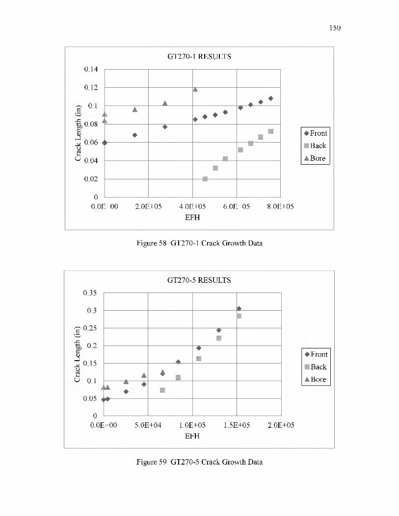
150
0.14
0.12
^ 0.1wt 0.08 8^ n da
GT270-1 RESULTS
A
A
♦ ♦ ♦AL
i ♦ ♦ ♦ ♦
♦♦ ■
■ Front
Back
Bore
^ 0.00 c ar
^ 0.04
0.02
00.0E
►
■
■■
■■
.+00 2.0E+05 4.0E+05 0.0E+05 8.0E+05EFH
Figure 58 GT270-1 Crack Growth Data
0.35
0.3
1 °.25
H 0.2ngeL
^ 0.15kcaarC 0.1
j0.05
A
GT270-5 RESULTS
♦■
♦■
♦■ Front
Back
BoreA ♦ .A ▲■
0.0E+00 5.0E+04 1.0E+05 1.5E+05 2.0E+05EFH
Figure 59 GT270-5 Crack Growth Data
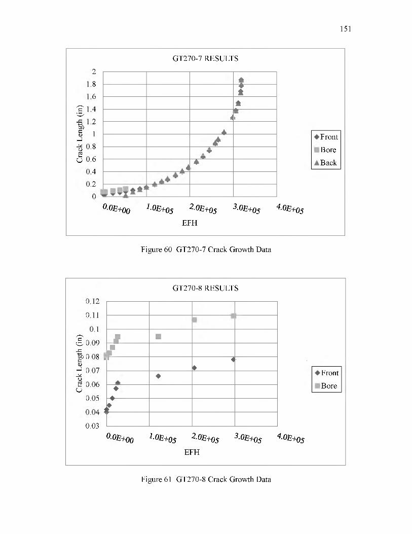
151
Crac
k Le
ngth
(in
)0.
0. 0.
0. 1.
1. 1.
1.0
2 4
6 8
1 2
4 6
8 2
GT270-7 RESULTS
♦t
±
iA ..................t
4,
*Front
Bore
Backv v
a 4*
' -
°OE+oo 1-OE+os ^-OE+os ^-OE+osEFH
4-OE+os
Figure 60 GT270-7 Crack Growth Data
Crac
k Le
ngth
(in
)0.
0. 0.
0. 0.
0 0.
0. 0
0 0
0 0
. 1
1i
Ui
(^
sI
OO
\O
hh
K)
h*.
n—1
GT270-8 RESULTS
1
| ■■
Pr «»
•
♦ Front
Bore♦▲▼
f
0.03
t
°°E+00 l °E+0s 2-OE+o5 3-OE+o5EFH
^■0E+0s
Figure 61 GT270-8 Crack Growth Data
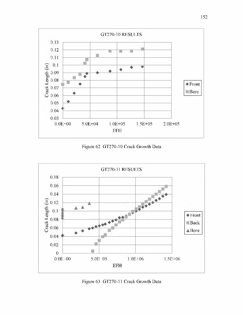
152
Crac
k Le
ngth
(in
)0.
0. 0.
0. 0.
0. 0
0. 0.
0. 0
0 0
0 0
0 .
1 1
10
4^
Ui
O'\
^1
00
VO
^^
K>
U>
-A. M
GT270-10 RESULTS
_ _ ■■■
■ ■
■■
* ♦ ♦ ♦ •
♦♦▼
i " ♦ Front
Bore♦
♦►
0.0E+00 5.0E+04 1.0E+05 1.5E+05 2.0E+05EFH
Figure 62 GT270-10 Crack Growth Data
GT270-11 RESULTS
0.18
0.16
0.14
3^ 0.12
hgt 0.1 e
J 0.08 kc
J 0.06
0.04
0.02
▲« A A
V
^ ♦ V» ♦♦
♦1■
■1
■00.0E+00
Front
Back
A Bore
5.0E+05 1.0E+06 1.5E+06EFH
Figure 63 GT270-11 Crack Growth Data
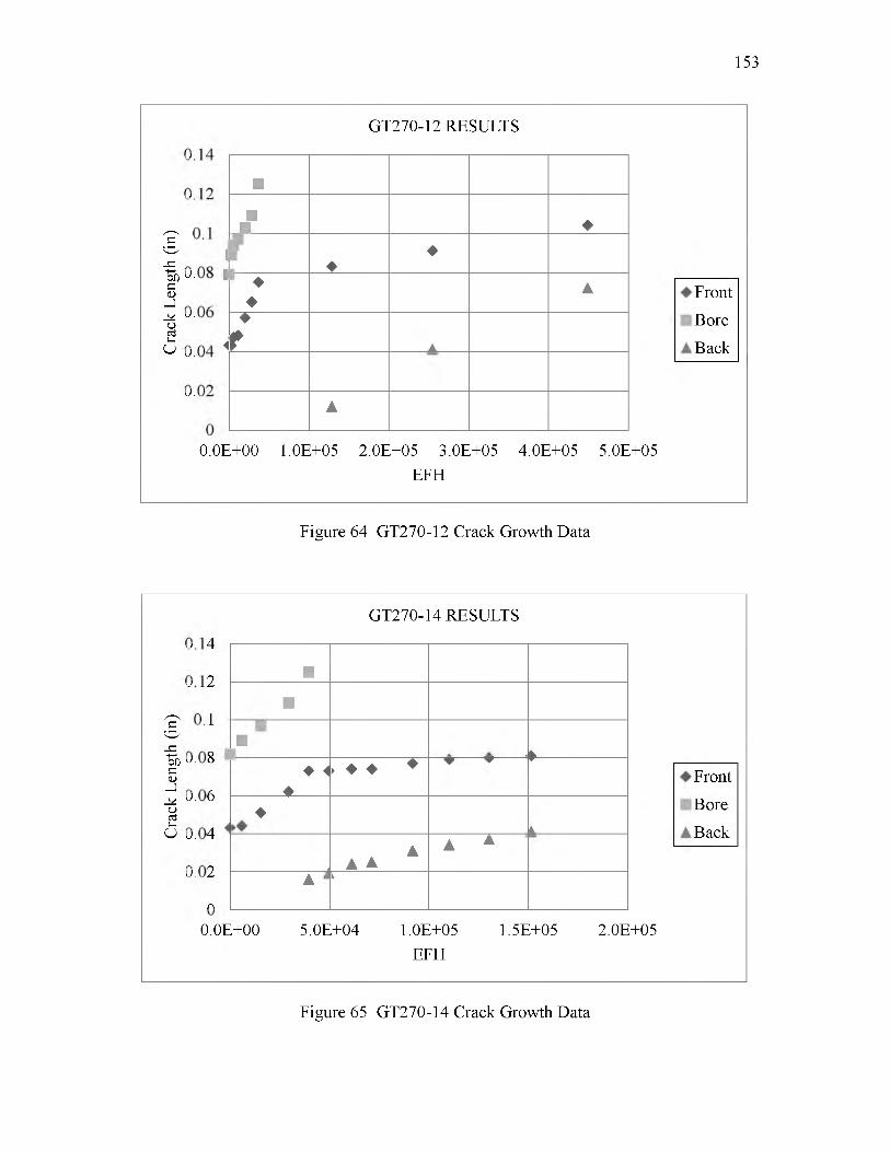
153
Crac
k Le
ngth
(in
)0.
0. 0.
0. 0
0. 0.
0 0
0 0
. 1
1
▲ ™
---
GT270-12 RESULTS
■
■■ ♦
♦♦
♦♦
▲ Front
Bore
Back
♦
t ▲
A
0.0E+00 1.0E+05 2.0E+05 3.0E+05 4.0E+05 5.0E+05EFH
Figure 64 GT270-12 Crack Growth Data
Crac
k Le
ngth
(in
)0.
0. 0.
0. 0
0. 0.
0 0
0 0
. 1
1 d
K)
-(
^o
no
o^
K)
4^
GT270-14 RESULTS
■
■
■t
♦ 4♦
> ♦ ♦ ♦ ▼ ▼Front
Bore
Back♦
kA
A AA *
A k
0.0E+00 5.0E+04 1.0E+05 1.5E+05 2.0E+05EFH
Figure 65 GT270-14 Crack Growth Data
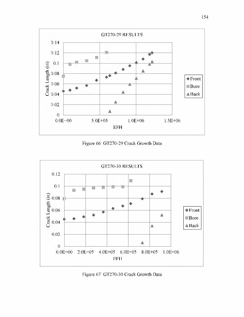
154
Crac
k Le
ngth
(in
)0.
0. 0.
0. 0
0. 0.
0 0
0 0
. 1
1^
K)
4^
0\
oo
^K
)4
^
GT270-29 RESULTS
▲. . " <
♦A
♦♦
T AA
1♦ ♦ ♦ . Front
Bore
Back
A
A
A
A
0.0E+00 5.0E+05 1.0E+06 1.5E+06EFH
Figure 66 GT270-29 Crack Growth Data
0.12
0.1
£ 0.08 | h htg
§ 0.06 L ko
£ 0.04 C
0.02
n
GT270-30 RESULTS
■
■ ■ ■ ■♦ ♦
1
♦ ♦
♦♦
Front
Bore
Back► ♦ ♦
♦ ♦ A
A
A
0.0E+00 2.0E+05 4.0E+05 6.0E+05 8.0E+05 1.0E+06EFH
Figure 67 GT270-30 Crack Growth Data
APPENDIX I
ADDITIONAL SEM IMAGES OF TEST SPECIMEN FRACTURE
SURFACES
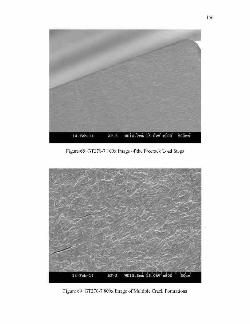
150
Figure 08 GT270-7 100x Image of the Precrack Load Steps
Figure 09 GT270-7 800x Image of Multiple Crack Formations

157
Figure 70 GT270-7 40x Image of Secondary Cracks Near End of Fatigue Crack
Figure 71 GT270-28 2,000x Precrack Surface Image
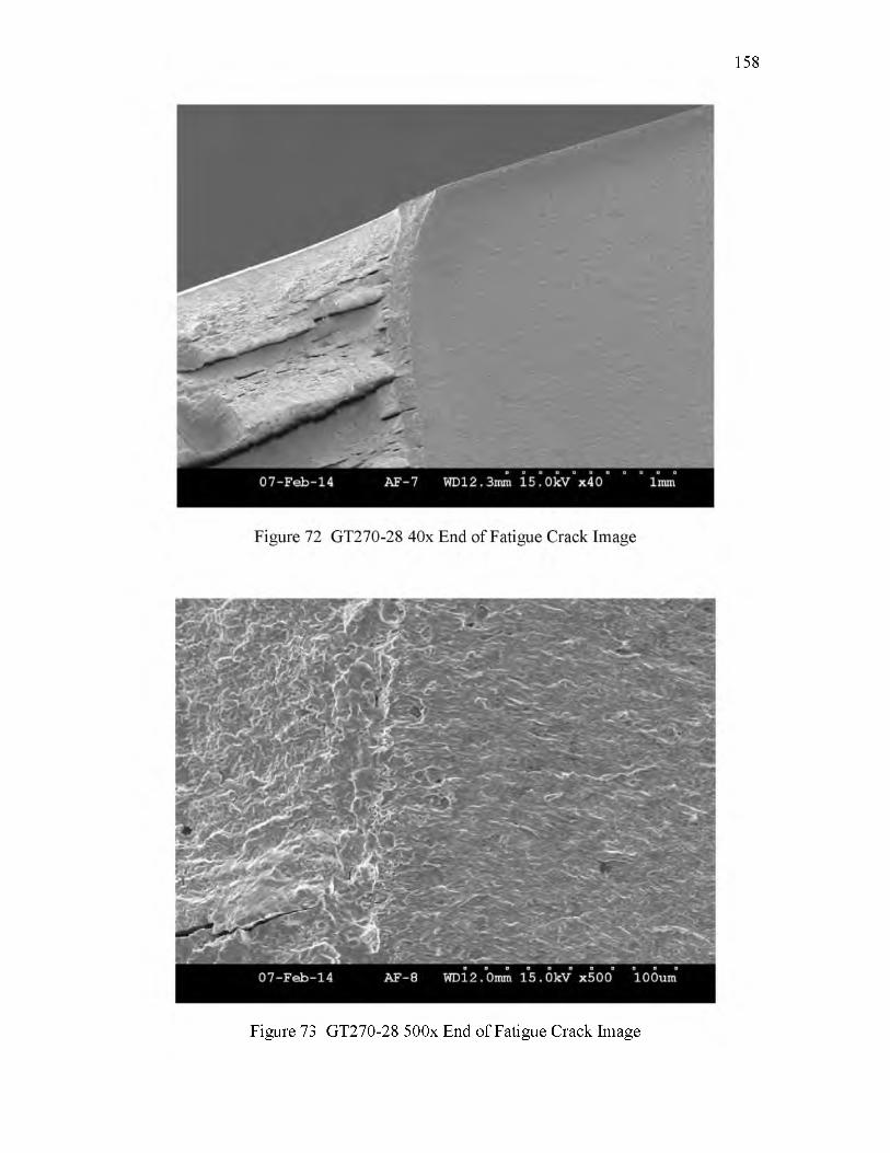
158
Figure 73 GT270-28 500x End of Fatigue Crack Image
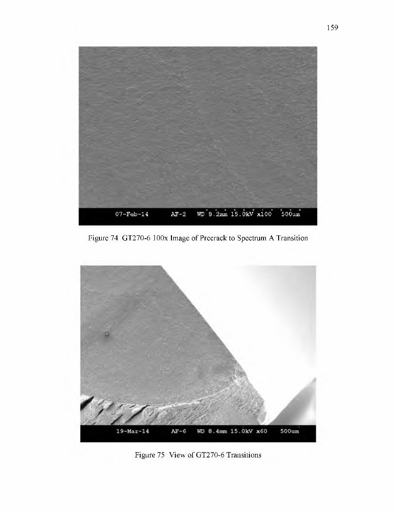
159
07-Feb-14 AF-2 WD" 8 .°2nun 15. OkV xi00° 5o6um
Figure 74 GT270-6 100x Image of Precrack to Spectrum A Transition
Figure 75 View of GT270-6 Transitions
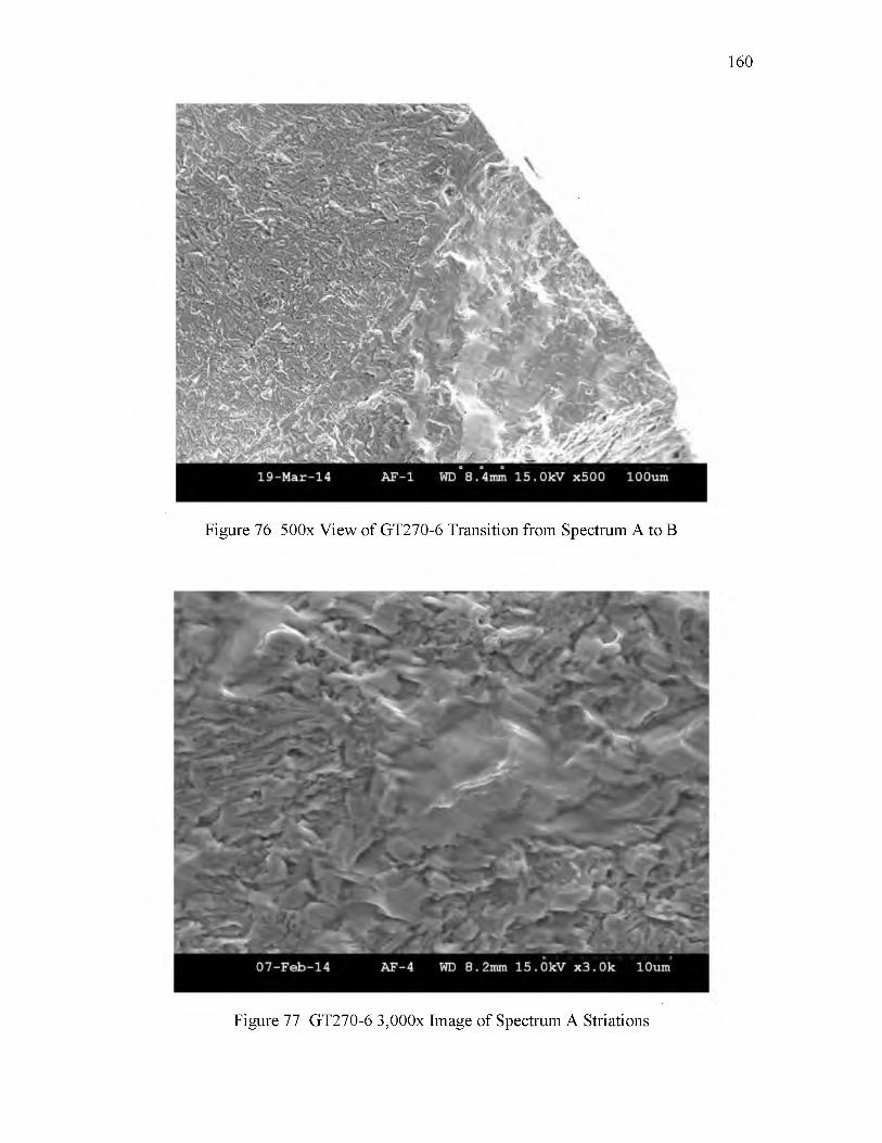
160
Figure 76 500x View of GT270-6 Transition from Spectrum A to B
Figure 77 GT270-6 3,000x Image of Spectrum A Striations
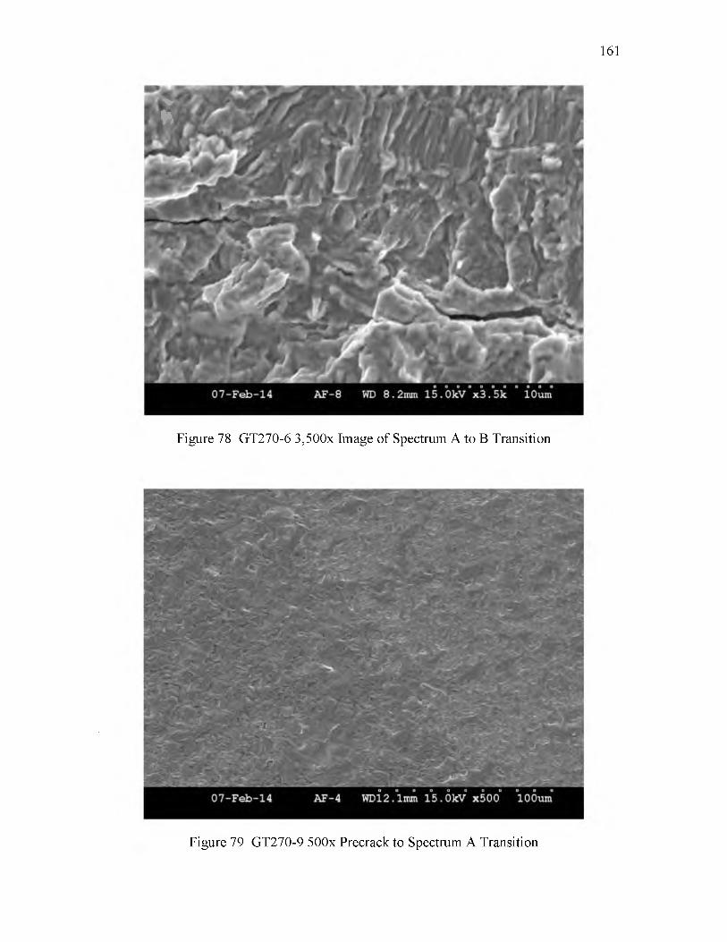
*4
161
Figure 78 GT270-6 3,500x Image of Spectrum A to B Transition
Figure 79 GT270-9 500x Precrack to Spectrum A Transition
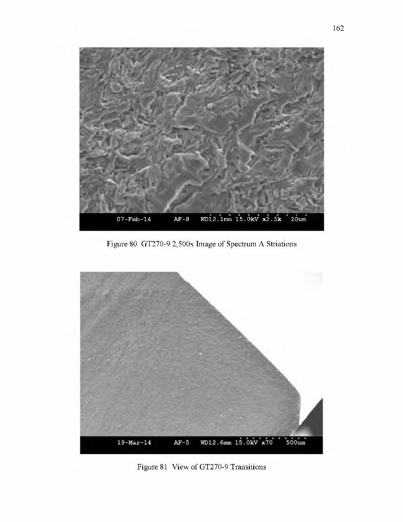
162
rL
/ r V V * f A *IHHiiHHWBK: y07-Feb-14 AF-8 Wd {2.1mm 15.OkV x2.5k 20um
Figure 80 GT270-9 2,500x Image of Spectrum A Striations
Figure 81 View of GT270-9 Transitions
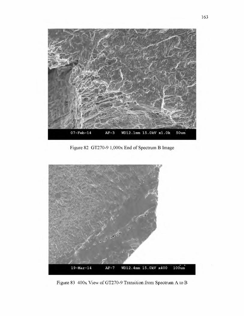
163
Figure 83 400x View of GT270-9 Transition from Spectrum A to B
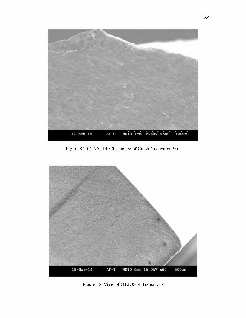
104
Figure 84 GT270-14 500x Image of Crack Nucleation Site
Figure 85 View of GT270-14 Transitions
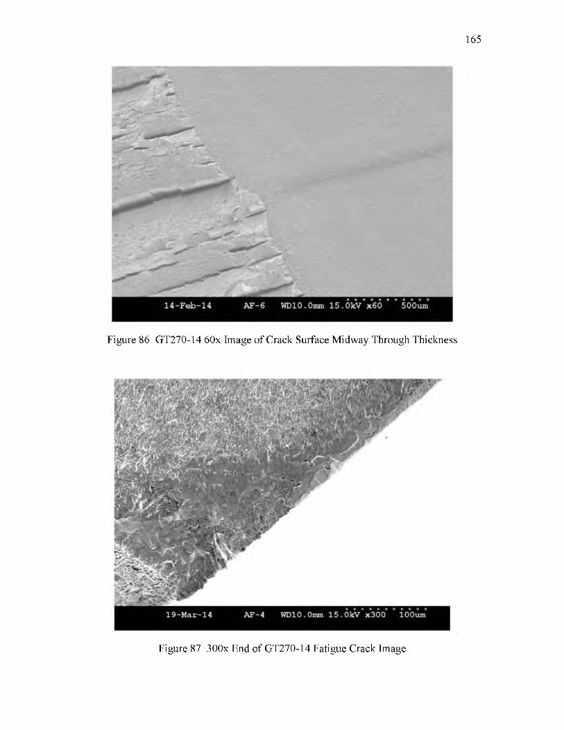
165
Figure 86 GT270-14 60x Image of Crack Surface Midway Through Thickness
Figure 87 300x End of GT270-14 Fatigue Crack Image
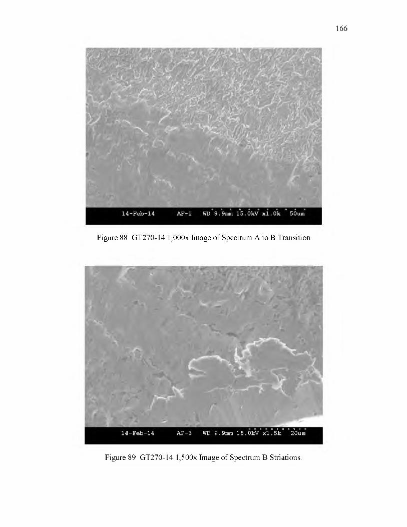
166
Figure 88 GT270-14 1,000x Image of Spectrum A to B Transition
14-Feb-14 AF-3 WD 9.9mm 15. OkV°xl !5°k° °2°0um
Figure 89 GT270-14 1,500x Image of Spectrum B Striations.

REFERENCES
[1] Boeing, "Commercial Airplanes Jet Prices," Boeing, 2014. [Online]. Available: http://www.boeing.com/boeing/commercial/prices. [Accessed 22 February 2014].
[2] United States Air Force, "F-16 Fighting Falcon Fact Sheet," United States Air Force, 15 October 2007. [Online]. Available:http://www.af.mil/AboutUs/FactSheets/Display/tabid/224/Article/104505/f-16-fighting- falcon.aspx. [Accessed 22 February 2014].
[3] Federation of American Scientists, "A-10/0A-10 Thunderbolt II," Federation of American Scientists, 2013. [Online]. Available:http://www.fas.org/programs/ssp/man/uswpns/air/attack/a10.html. [Accessed 11 November 2013].
[4] United States Air Force, "B-52 Stratofortress FactSheet," United States Air Force, 20 September 2005. [Online]. Available:http://www.af.mil/AboutUs/FactSheets/Display/tabid/224/Article/104465/b-52- stratofortress.aspx. [Accessed 11 November 2013].
[5] American Society for Testing Materials, "ASTM E1823 Standard Terminology Relating to Fatigue and Fracture Testing," 1 February 2013. [Online]. Available: http://specs4.ihserc.com/Document/Document/ViewDoc?docid=ZFRBDFAAAAAAAAAA. [Accessed 20 March 2014].
[6] H. A. Wood and R. M. Engle, USAF Damage Tolerant Design Handbook: Guidelines for the Analysis and Design of Damage Tolerant Aircraft, Wright-Patterson Air Force Base, OH: United States Air Force, 1979.
[7] Department of Defense, "MIL-STD-1530 Standard Practice Aircraft Structural Integrity Program (ASIP)," 1 November 2005. [Online]. Available:http://specs4.ihserc.com/Document/Document/ViewDoc?docid=ZLQOIBAAAAAAAAAA. [Accessed 20 March 2014].
108
[8] M. Levy, "Test Plan - Fatigue Crack Evaluation of Training vs. Non Training Missions," Northrop Grumman Aerospace Systems, Bethpage, NY, 2013.
[9] J. Mackerelle, Fatigue Crack Evaluation o f Training versus Non-Training Missions Development o f Non-Training Mission Maneuver Spectrum, 2012.
[10] R. Beal, "Spectrum Comparison of an Extended Service Life System using 2024-T351 Aluminum," University of Utah, Salt Lake City, UT, 2014.
[11] J. Kokoris, "Spectrum Usage and Development," Northrop Grumman Aerospace Systems, Bethpage, NY, 2000.
[12] M. Janssen, J. Zuidema and R. Wanhill, Fracture Mechanics 2nd Edition, Delft, The Netherlands: VSSD, 2000.
[13] J. Schijve, "Observations on the Prediction of Gatigue Crack Growth Propagation Under Variable-Amplitude Loading," in Fatigue Crack Growth Under Spectrum Loads, Philidelphia, PA, American Society for Testing and Materials, 1970, pp. 3-23.
[14] P. J. Bernard, T. C. Lindley and C. E. Richards, "Mechanisms of Overload Retardation During Fatigue Crack Propagation," in Fatigue Crack Growth Under Spectrum Loads, Philidelphia, PA, American Society for Testing and Materials, 1970, pp. 78-97.
[15] W. X. Alzos, A. C. Skat and B. M. Hillberry, "Effect of Single Overload/Underload Cycles on Fatigue Crack Propagation," in Fatigue Crack Growth Under Spectrum Loads, Philidelphia, PA, American Society for Testing and Materials, 1970, pp. 27-40.
[10] R. I. Stephens, D. K. Chen and B. W. Hom, "Fatigue Crack Growth with Negative Stress Ratio Following Single Overloads in 2024-T3 and 7075-T0 Aluminum Alloys," in Fatigue Crack Growth Under Spectrum Loads, Philidelphia, PA, American Society for Testing and Materials, 1970, pp. 27-40.
[17] J. Reiman, M. Landy and M. Kaplan, "Effect of Spectrum Type on Fatigue Crack Growth Life," in Fatigue Crack Growth Under Spectrum Loads, Philadelphia, PA, American Society for Testing and Materials, 1970, pp. 187-202.
[18] W. Zhuang, S. Barter and L. Molent, "Flight-by-flight fatigue crack growth life assessment," International Journal o f Fatigue, vol. 29, no. 9, pp. 1047-1057, 2007.
169
[19] S. U. Khan, R. C. Alderliesten, J. Schijve and R. Benedictus, "On the fatigue crack growth prediction under variable amplitude loading," in Computational and experimental analysis of damaged materials, Delft, The Netherlands, Delft University of Technology, 2007, pp. 77105.
[20] S. Kalnaus, F. Fan, Y. Jiang and A. Vasudevan, "An experimental investiation of fatigue crack growth of stainless steel 304L," International Journal o f Fatigue, vol. 31, pp. 840-849, 2009.
[21] L. Smith, "The Generalized Willenborg Shutoff Overload Ratio and Its Sensitivity to Analytical Parameteres and Techniques," Southwest Research Institute, San Antonio, TX, 2006.
[22] J. Willenborg, H. A. Wood and R. M. Engle, "A crack growth retardation model using an effective stress concept," Air Force Flight Dynamics Laboratory, Wright Patterson Air Force Base, OH, 1971.
[23] ASM International, Metal Handbook Desk Edition, Russell Township, OH: ASM International, 1998.
[24] SAE International, "SAE AMS5528 Steel, Corrosions - Resistant, Sheet, Strip, and Plate 17Cr - 7.1 Ni - 1.1 Al Solution Heat treated, Precipitation Hardenable," October 2012. [Online]. Available:http://specs4.ihserc.com/Document/Document/ViewDoc?docid=WRRQAFAAAAAAAAAA. [Accessed 20 March 2014].
[25] Northrop Grumman Corporation, "Mechanical Properties of 17-7 PH Test Material,"Northrop Grumman, Bethpage, New York, 2012.
[26] D. Andrew, "Investigation of Cold Expansion of Short Edge Margin Holes with Pre-existing Cracks in 2024-T351 aluminum Alloy," University of Utah, Salt Lake City, UT, 2011.
[27] Gaertner Scientific Corporation, Packing List, Chicago, IL: Gaertner, 2010.
[28] American Society for Testing and Materials, "ASTM E647 Standard Test Method for Measurement of Fatigue Crack Growth Rates," 15 October 2013. [Online]. Available: http://specs4.ihserc.com/Document/Document/ViewDoc?docid=ONKMHFAAAAAAAAAA. [Accessed 20 March 2014].
[29] G. C. Sih, Handbook of Stress-Intensity Factors, Bethlehem, PA: Institute of Fracture and Solid Mechanics at Lehigh University, 1973.

170
[30] J. Harter, AFGROW Users Guide and Technical Manual, Centerville, OH: LexTech, 2010.
[31] R. Pilarczyk and T. Allred, "Damage Tolerance Analysis Ground Rules," A-10 ASIP Group, Hill AFB, UT, 2010.
[32] SAE International, "AMS 2759/3E Heat Treatment Precipitation-Hardening Corrosion- Resistant and Maraging Steel part," 08 2008. [Online]. Available:http://sape4.ihserc.com/Document/Document/ViewDoc?docid=CTWAHCAAAAAAAAAA. [Accessed 18 04 2014].