Embed Size (px)
Citation preview
Computational Statistics & Data Analysis 52 (2007) 325–334www.elsevier.com/locate/csda
A stochastic approximation view of boosting
C. Andy Tsaoa,∗, Yuan-chin Ivan Changb,c
aDepartment of Applied Mathematics, National Dong Hwa University, TW 97401, TaiwanbInstitute of Statistical Science, Academia Sinica, Taipei, TW 11529, Taiwan
cDepartment of Statistics, National Chengchi University, Taipei, TW 11605, Taiwan
Available online 1 July 2007
Abstract
The boosting as a stochastic approximation algorithm is considered. This new interpretation provides an alternative theoreticalframework for investigation. Following the results of stochastic approximation theory a stochastic approximation boosting algorithm,SABoost, is proposed. By adjusting its step sizes, SABoost will have different kinds of properties. Empirically, it is found thatSABoost with a small step size will have smaller training and testing errors difference, and when the step size becomes large, ittends to overfit (i.e. bias towards training scenarios). This choice of step size can be viewed as a smooth (early) stopping rule. Theperformance of AdaBoost is compared and contrasted.© 2007 Elsevier B.V. All rights reserved.
Keywords: Boosting; Stochastic approximation; Robbins–Monro procedure; Smooth early stopping
1. Introduction
Boosting is one of the successful ensemble classifiers and has attracted much attention recently. Earlier theoreticalresults show that boosting reduces the training error under the weak base hypothesis assumption and upper bounds ofits testing errors can be obtained in some PAC (probably approximately correct) sense, see, for example, Freund andSchapire (1997). Boosting is also recognized as a large margin algorithm, see, for example, Schapire et al. (1998) andBreiman (1999). It has been observed that boosting is relatively resistant to overfitting in many practical applications withless noisy data. These empirical successes motivate theoretical investigations of possible explanations. See, for example,Schapire (1990), Grove and Schuurmans (1998), Freund and Schapire (1997), Friedman et al. (2000), Schapire et al.(1998) and Jiang (2002). The readers are referred to Meir and Rätsch (2003) for a review of more recent advancements.Recent studies provide a much clearer picture of Bayes consistency of boosting. Breiman (2004) shows that populationversion boosting is Bayes consistent and Jiang (2004) shows boosting is process consistent for the sample version.Other asymptotic aspects are also studied, for example Bühlmann andYu (2003) and Zhang andYu (2005). More recentstudies can be found in, for example, Leitenstorfer and Tutz (2007), Merler et al. (2007), Tutz and Binder (2006), Geyand Poggi (2006) and Kim and Koo (2005,2006).
Although there are many modifications and interpretations of the original AdaBoost, many of its features remainunclear. The more we know about its properties, the more we can exploit its power. In this paper, the boosting-like algorithms are viewed as stochastic approximation procedures. Particularly, these algorithms are rendered by
∗ Corresponding author.E-mail addresses: [email protected] (C.A. Tsao), [email protected] (Y.-c.I. Chang).
0167-9473/$ - see front matter © 2007 Elsevier B.V. All rights reserved.doi:10.1016/j.csda.2007.06.020
326 C.A. Tsao, Y.-c.I. Chang / Computational Statistics & Data Analysis 52 (2007) 325–334
the Robbins–Monro (RM) procedure in Robbins and Monro (1951). This stochastic approximation viewpoint is thencontrasted with the interpretation of (Discrete) AdaBoost given in Friedman et al. (2000).
Robbins and Monro (1951) develops and analyzes a recursive procedure for finding the root of a real-value functiong(·) of a real variable �. This function is assumed to be unknown, but noise-corrupted observations could be takenat values of � selected by the experimenter. If the function g(·) were known and continuously differentiable, thenfinding its roots becomes a classical problem in numerical analysis. Various procedures such as Newton’s method havebeen proposed in this case. However, when the observation is noise-corrupted, these procedures might not work well.Many modifications and alternatives have been introduced to account for noise. RM procedure and Kiefer–Wolfowitz(KW) procedure, respectively, proposed in Robbins and Monro (1951) and Kiefer and Wolfowitz (1952) are two ofthe most well-known procedures being proposed under stochastic approximation frameworks. For simplicity, only therendering based on the deterministic RM procedure will be discussed. The relations of boosting-like algorithms to othermodifications of the RM and KW procedures will be reported elsewhere.
Following the convergence theorem of the RM procedure, we propose a stochastic approximation boosting algorithm,SABoost. By adjusting the step size of SABoost, it will have different properties. Empirically, if a large step size ischosen, the training errors of SABoost will decrease quickly and tend to overfit. On the other hand, when a small stepsize is chosen, the training errors decrease slowly, and the phenomena of overfitting becomes negligible. In addition,the SABoost with small step size is more stable than AdaBoost in the sense that no drastic change of training and testingerrors presents during boosting iterations.
The rest of this paper is organized as follows. In order to redescribe AdaBoost using a stochastic approxima-tion procedure, we will first review AdaBoost and the RM procedure in Sections 2 and 3, respectively. The conver-gence theorem of the RM procedure is stated in Section 3. Empirical results of some benchmark and the synthesizeddata sets are shown in Section 4. Concluding remarks, discussion and some possible future studies are given inSection 5.
2. FHT’s interpretation
Boosting (refer Freund and Schapire, 1997; Schapire, 1990, for more details) is a learning procedure that startswith a weak base learner and assigns the misclassified data higher weights in each iteration. Then it takes a weightedmajority vote to predict labels of examples with given feature variables. The process is then repeated T iterations. ThisT is known as the boosting time and can be configured by users for early stopping. Although many variations and mod-ifications of boosting have been proposed over the years, here we will mainly focus on the Discrete AdaBoost for easyexposition.
To fix notations, let us consider a supervised learning problem with binary responses where training data (xi, yi)n1,
testing data (x′j , y′j )m1 and yi, y
′j= ∈ Y= {±1} are given. Here x’s and x′’s are “input” or “explanatory” variables and
y’s and y′’s are output or response variables. It is desired to find a good machine or classifier F based on the informationof training data such that F can predict y′ for each x′ as correctly as possible. Usually the performance of F is measuredthrough its training error (TE) and testing/generalization error (GE) defined as
TE= 1
n
∑i
1[yi �=F(xi )] and GE= 1
m
∑j
1[y′j �=F(x′j )].
Note that it is often assumed that X and Y arised from some (unknown) joint distribution. Rigorously, testing errorshould be EY,X1[Y �=F(X)] rather than GE we defined above. However, the sampling analog GE can be considered as anestimate of EY,X1[Y �=F(X)]. For large m, GE is a satisfactory estimator in the sense of (statistical) consistency.
Now, the Discrete AdaBoost algorithm:
Discrete AdaBoost.
(1) Start with weights Dt(i)= 1/n, i = 1 to n.(2) Repeat for t = 1 to T
• Obtain ht (x) from weak learner h using weighted training data with respect to Dt .• Compute �t = EDt 1[y �=ht (x)], �t = log 1−�t
�t.
C.A. Tsao, Y.-c.I. Chang / Computational Statistics & Data Analysis 52 (2007) 325–334 327
• Update i = 1 to n,
Dt+1(i)= 1
Zt
Dt(i) exp[�t1[yi �=ht (xi )]],where Zt is the normalizer.
(3) Output the classifier F(x)= sgn[∑Tt=1�t ht (x)].
Friedman et al. (2000) (FHT) show that
Remark 1. The Discrete AdaBoost (population version) builds an additive logistic regression model via Newton-likeupdates for minimizing E(e−YF(X)).
This is an insightful and powerful observation. Immediately, it motivates construction of new boosting-like algorithmsand provides a statistical framework for further theoretical investigations.
Specifically, let Y ∈ {±1} denote the labels and X be the domain of feature variables. Suppose F is a real-valuedfunction mapping X to R. Then in binary classification problems, our goal is to predict Y by the sign of estimatedF based on a set of labeled examples. Friedman et al. (2000) render AdaBoost as a Newton update minimizing anapproximate risk J (F ) ≡ EX,Y [e−YF(X)] ≈ EX,Y 1[YF(X)<0] and obtain the update formula
F(x)← F(x)+ 1
2log
(1− err
err
)f (x), (1)
w(x, y)← w(x, y) exp
[log
(1− err
err
)1[y �=f (x)]
], (2)
where f (x)= sgn(Ew(Y |x)) and err= Ew[1[Yf (x)<0]|x].Alternatively,
Ft+1(x)= Ft(x)+ �t f (x), (3)
where �t = 12 log( 1−�t
�t), wt(x, y)= exp(−yF t (x)), Ewt g(x, Y ) denotes EY |x[wt(x, Y )g(x, Y )]/(EY |xwt (x, Y )) and
�t = Ewt 1[yf (x)<0].Note that this interpretation is based on minimization of an (approximated) conditional risk where X is given.
Furthermore, it is in nature a population-version theory in the sense that X andY are considered as random vector/variable.And when X is conditioned, the optimization problem is essentially a problem of sample size 1. This conditional riskapproach greatly simplifies the theoretical analysis.
3. Stochastic approximation
Minimization of conditional risk is hardly a new task for statisticians. Specifically, now the objective is to find F∗such that
F∗(x)= arg minF(x)
�(F (x)) (4)
where �(F (x))= EY |xL(Y, F (x)). Under some regularity conditions, this F∗ is also a solution to
�(F (x)) ≡ �′(F (x))= EY |xL
′(Y, F (x))= 0 (5)
where L′(Y, F )= �L(Y, F )/�F . This problem has long been studied from a stochastic approximation viewpoint. See
Lai (2003) for a review on stochastic approximation. We consider here the most well-known RM procedure and restatethe RM deterministic (RM-D) algorithm given in Duflo (1997) in our current context and notations. The readers arereferred to Duflo (1997) and Robbins and Monro (1951) for their original formulation.
RM-D Algorithm.
• Choose F0 arbitrarily.
328 C.A. Tsao, Y.-c.I. Chang / Computational Statistics & Data Analysis 52 (2007) 325–334
• Iterate t = 0, 1, . . . ,
gt+1(x)= �(Ft (x)),
Ft+1(x)= Ft(x)− �t (gt+1 + �t+1), �t , �t+1 �0.
Note that in usual boosting-like algorithms, there is no �t terms, that is, �t = 0. However, as we will see immediatelyin the coming proposition, with suitable regularization, such �’s can be introduced without affecting the convergence.
Although Friedman et al. (2000) provide a good interpretation of boosting, their Result 1 leaves us no guidance abouthow to check the convergence of Newton updates. In contrast, the convergence of stochastic approximation algorithmshave been established under various conditions. The following proposition is an adaption of the convergence theoremof the RM-D algorithm; for example, see Sections 1.2 and 1.4 in Duflo (1997). Here we restate Proposition 1.2.3 inDuflo (1997) in our notations. Note that the dependency of x is notationally suppressed.
Proposition 2 (RM-D convergence). If � is a monotonic continuous real function such that �(F∗)= 0 and for all F
�(F ) (F − F∗) > 0,
|�(F )|�K(1+ |F |) for some K .
Suppose {�t }, {�t } are two sequences of real numbers and �t �0. Define
Ft+1 = Ft − �t (�(Ft )+ �t+1). (6)
If �t decreases to 0 such that∑
t
�t =∞;∑
t
�t�t <∞, (7)
then Ft converges to F∗ for any initial F0.
Sequences �t and �t control the speed of approximation of the stochastic approximation algorithm. In particular, �t
controls the “step size” of stochastic approximation. The common choice for �t is �/t and �t = 0, with some � > 0.When the exponential criterion is employed, that is L(Y, F )= e−YF , and then L′(Y, F )=−Y e−YF , the algorithms
can be further simplified and render forms similar to the original AdaBoost.
RM-D Algorithm with Exponential Criterion.
• Choose F0 arbitrarily.• Iterate t = 0, 1, . . . ,
gt+1(x)= − EY |xY exp(−YF t (x))
Ft+1(x)= Ft(x)− �t gt+1(x)
= Ft(x)+ �t (EY |xwt (x, Y ))Ewt (Yt+1|x), �t �0 (8)
where wt(x, y)= exp(−yF t (x)) and again
Ewt g(x, Y )= EY |x[wt(x, Y )g(x, Y )]EY |xwt (x, Y )
.
The original form (6) suggests our approach is closely related to Friedman (2001,2002) since the gradient of theconditional risk is employed in updating iteration. However, Friedman (2001,2002) are of the sample-version theories.Both account for the finite sample in choosing the optimal parameters in the classifier F. Furthermore, the form ofthe possible classifiers are explicitly given as the addition of some simple functions (base learners). Our approachis a population-version theory. Our formulation is more related to Friedman et al. (2000). This approach does notspecify the explicit form of the classifiers and therefore not directly allows optimization of the parameters. Althoughthis population approach simplifies the notations and analytical derivation, it provides no clear guideline as how to use
C.A. Tsao, Y.-c.I. Chang / Computational Statistics & Data Analysis 52 (2007) 325–334 329
the data and how to utilize the base learners. Nonetheless, our results suggest stochastic approximation can serve as analternative framework for investigating boosting-like algorithms.
The iterative algorithms (8) and (3) bear formal similarity. Under the conditions of Proposition 2 the convergenceof (8) can be established. On the hand, the convergence of the population-version Discrete AdaBoost (3) is less clear.It should be noted that the population-version results do not imply the corresponding algorithms will have the sameconvergence when working with finite sample data.
It follows from Proposition 2 that we can manipulate sequences {�t }, {�t } such that the boosting procedures will havedifferent kinds of properties. These properties will be illustrated with some bench mark data sets and synthesized data inthe next section. In contrast with the original AdaBoost, we call this procedure SABoost. SABoost is similar to DiscreteAdaBoost except that the “step size” �t is replaced by st = �tEY |xwt (x, Y ) where �t = �/t for some � > 0. This choiceof �t is also supported by a widely stated sufficient condition for convergence of a stochastic approximation procedure
∞∑t=1
�t =∞;∞∑t=1
�2t <∞ (9)
under quite general settings. See, for example, Duflo (1997). With choices of � and thus the step size, SABoost canhave quite different performances.
4. Empirical results
4.1. Bench mark data sets
For evaluating the performances of SABoost, we conduct experiments with both synthesized and some bench markdata sets. Here we first compare the performances of SABoost with Discrete AdaBoost with decision stumps (DS) asbase learners for both procedures. Different step sizes are used in SABoost. In our experiments, we set �t = 0, �t = �/t
and � > 0 is a positive real number and choose �=0.5, 1, and 1.5. All experiments are done on PC’s running Window XPsystem. The statistical programming language R is used for all experiments. (cf. Verzani, 2005, and www.r-project.orgfor the details of language R.)
In order to prevent the slow convergence rate of SABoost due to the small step size �, we propose a hybrid procedurecombining SABoost and AdaBoost together in the following way: (1) Let T be the pre-chosen total iteration numberand conduct the original Discrete AdaBoost procedure in the first [ ∗ T ] ( ∈ (0, 1)) iterations, where [A], A ∈ R,denotes the largest integer less than A. (2) Switch to SABoost for the rest T − [ ∗ T ] of iterations. It will be calledHybrid SABoost here. In all our experiments, we set = 0.25. Specifically
SABoost. (1) Start with weights Dt(i)= 1/n, i = 1 to n and Ct = 1.
(2) Repeat for t = 1 to T
• Obtain ht (x) from weak learner h using weighted training data with respect to Dt .• Compute �t = EDt 1[y �=ht (x)], st = sgn(0.5− �t )�t ∗ Ct .
• Update i = 1 to n,
Dt+1(i)= 1
Zt
Dt(i) exp[st1[yi �=ht (xi )]],
where Zt is the normalizer.• Update Ct =
( 1n
∑ni=1 exp[−yi ∗ Ft(xi)]
)−1
(3) Output the classifier F(x)= sgn[∑Tt=1stht (x)].
Hybrid-SABoost. (1) Start with weights Dt(i)= 1/n, i = 1 to n and Ct = 1.
(2) Repeat for t = 1 to [ ∗ T ]• Obtain ht (x) from weak learner h using weighted training data with respect to Dt .• Compute �t = EDt 1[y �=ht (x)], st = log 1−�t
�t.
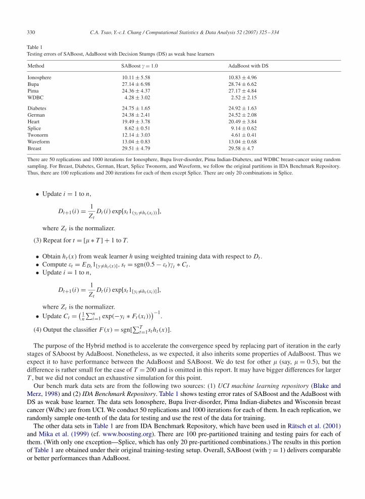
330 C.A. Tsao, Y.-c.I. Chang / Computational Statistics & Data Analysis 52 (2007) 325–334
Table 1Testing errors of SABoost, AdaBoost with Decision Stumps (DS) as weak base learners
Method SABoost �= 1.0 AdaBoost with DS
Ionosphere 10.11± 5.58 10.83± 4.96Bupa 27.14± 6.98 28.74± 6.62Pima 24.36± 4.37 27.17± 4.84WDBC 4.28± 3.02 2.52± 2.15
Diabetes 24.75± 1.65 24.92± 1.63German 24.38± 2.41 24.52± 2.08Heart 19.49± 3.78 20.49± 3.84Splice 8.62± 0.51 9.14± 0.62Twonorm 12.14± 3.03 4.61± 0.41Waveform 13.04± 0.83 13.04± 0.68Breast 29.51± 4.79 29.58± 4.7
There are 50 replications and 1000 iterations for Ionosphere, Bupa liver-disorder, Pima Indian-Diabetes, and WDBC breast-cancer using randomsampling. For Breast, Diabetes, German, Heart, Splice Twonorm, and Waveform, we follow the original partitions in IDA Benchmark Repository.Thus, there are 100 replications and 200 iterations for each of them except Splice. There are only 20 combinations in Splice.
• Update i = 1 to n,
Dt+1(i)= 1
Zt
Dt(i) exp[st1(yi �=ht (xi ))],
where Zt is the normalizer.
(3) Repeat for t = [ ∗ T ] + 1 to T.
• Obtain ht (x) from weak learner h using weighted training data with respect to Dt .• Compute �t = EDt 1[y �=ht (x)], st = sgn(0.5− �t )�t ∗ Ct .
• Update i = 1 to n,
Dt+1(i)= 1
Zt
Dt(i) exp[st1[yi �=ht (xi )]],
where Zt is the normalizer.• Update Ct =
( 1n
∑ni=1 exp(−yi ∗ Ft(xi))
)−1.
(4) Output the classifier F(x)= sgn[∑Tt=1stht (x)].
The purpose of the Hybrid method is to accelerate the convergence speed by replacing part of iteration in the earlystages of SAboost by AdaBoost. Nonetheless, as we expected, it also inherits some properties of AdaBoost. Thus weexpect it to have performance between the AdaBoost and SABoost. We do test for other (say, = 0.5), but thedifference is rather small for the case of T = 200 and is omitted in this report. It may have bigger differences for largerT , but we did not conduct an exhaustive simulation for this point.
Our bench mark data sets are from the following two sources: (1) UCI machine learning repository (Blake andMerz, 1998) and (2) IDA Benchmark Repository. Table 1 shows testing error rates of SABoost and the AdaBoost withDS as weak base learner. The data sets Ionosphere, Bupa liver-disorder, Pima Indian-diabetes and Wisconsin breastcancer (Wdbc) are from UCI. We conduct 50 replications and 1000 iterations for each of them. In each replication, werandomly sample one-tenth of the data for testing and use the rest of the data for training.
The other data sets in Table 1 are from IDA Benchmark Repository, which have been used in Rätsch et al. (2001)and Mika et al. (1999) (cf. www.boosting.org). There are 100 pre-partitioned training and testing pairs for each ofthem. (With only one exception—Splice, which has only 20 pre-partitioned combinations.) The results in this portionof Table 1 are obtained under their original training-testing setup. Overall, SABoost (with �= 1) delivers comparableor better performances than AdaBoost.
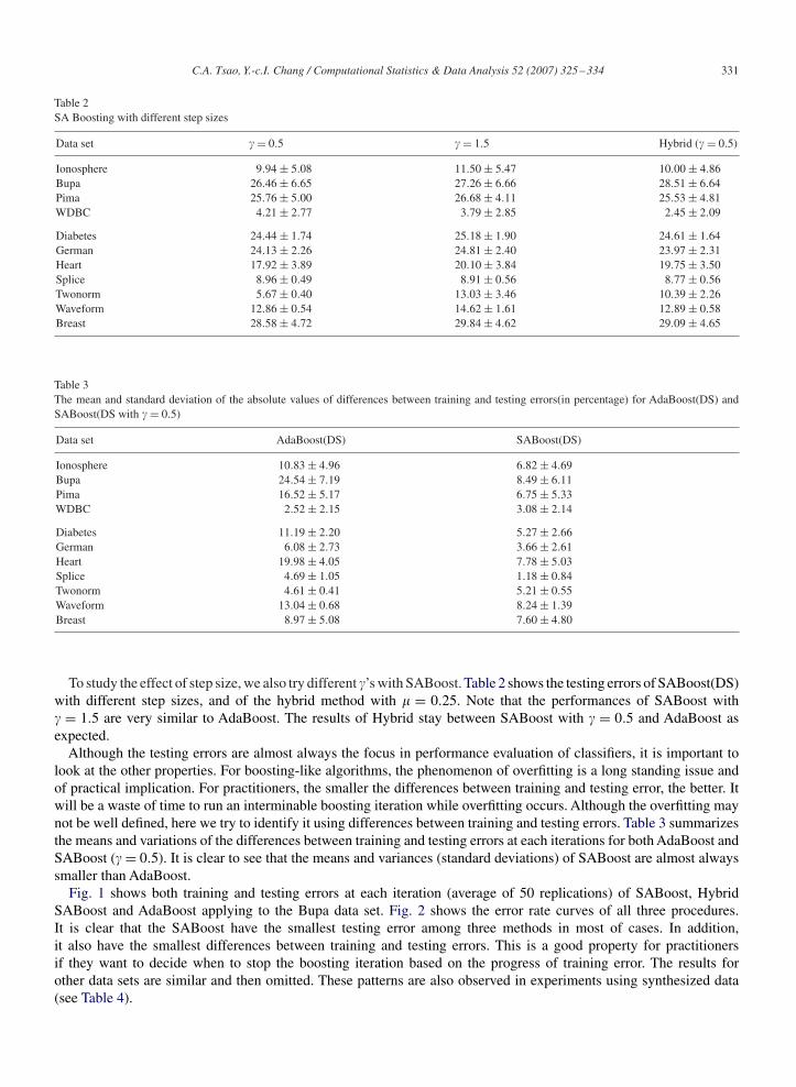
C.A. Tsao, Y.-c.I. Chang / Computational Statistics & Data Analysis 52 (2007) 325–334 331
Table 2SA Boosting with different step sizes
Data set �= 0.5 �= 1.5 Hybrid (�= 0.5)
Ionosphere 9.94± 5.08 11.50± 5.47 10.00± 4.86Bupa 26.46± 6.65 27.26± 6.66 28.51± 6.64Pima 25.76± 5.00 26.68± 4.11 25.53± 4.81WDBC 4.21± 2.77 3.79± 2.85 2.45± 2.09
Diabetes 24.44± 1.74 25.18± 1.90 24.61± 1.64German 24.13± 2.26 24.81± 2.40 23.97± 2.31Heart 17.92± 3.89 20.10± 3.84 19.75± 3.50Splice 8.96± 0.49 8.91± 0.56 8.77± 0.56Twonorm 5.67± 0.40 13.03± 3.46 10.39± 2.26Waveform 12.86± 0.54 14.62± 1.61 12.89± 0.58Breast 28.58± 4.72 29.84± 4.62 29.09± 4.65
Table 3The mean and standard deviation of the absolute values of differences between training and testing errors(in percentage) for AdaBoost(DS) andSABoost(DS with �= 0.5)
Data set AdaBoost(DS) SABoost(DS)
Ionosphere 10.83± 4.96 6.82± 4.69Bupa 24.54± 7.19 8.49± 6.11Pima 16.52± 5.17 6.75± 5.33WDBC 2.52± 2.15 3.08± 2.14
Diabetes 11.19± 2.20 5.27± 2.66German 6.08± 2.73 3.66± 2.61Heart 19.98± 4.05 7.78± 5.03Splice 4.69± 1.05 1.18± 0.84Twonorm 4.61± 0.41 5.21± 0.55Waveform 13.04± 0.68 8.24± 1.39Breast 8.97± 5.08 7.60± 4.80
To study the effect of step size, we also try different �’s with SABoost. Table 2 shows the testing errors of SABoost(DS)with different step sizes, and of the hybrid method with = 0.25. Note that the performances of SABoost with� = 1.5 are very similar to AdaBoost. The results of Hybrid stay between SABoost with � = 0.5 and AdaBoost asexpected.
Although the testing errors are almost always the focus in performance evaluation of classifiers, it is important tolook at the other properties. For boosting-like algorithms, the phenomenon of overfitting is a long standing issue andof practical implication. For practitioners, the smaller the differences between training and testing error, the better. Itwill be a waste of time to run an interminable boosting iteration while overfitting occurs. Although the overfitting maynot be well defined, here we try to identify it using differences between training and testing errors. Table 3 summarizesthe means and variations of the differences between training and testing errors at each iterations for both AdaBoost andSABoost (�= 0.5). It is clear to see that the means and variances (standard deviations) of SABoost are almost alwayssmaller than AdaBoost.
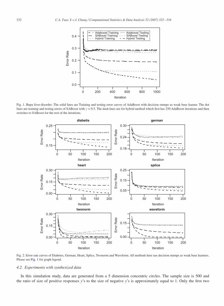
Fig. 1 shows both training and testing errors at each iteration (average of 50 replications) of SABoost, HybridSABoost and AdaBoost applying to the Bupa data set. Fig. 2 shows the error rate curves of all three procedures.It is clear that the SABoost have the smallest testing error among three methods in most of cases. In addition,it also have the smallest differences between training and testing errors. This is a good property for practitionersif they want to decide when to stop the boosting iteration based on the progress of training error. The results forother data sets are similar and then omitted. These patterns are also observed in experiments using synthesized data(see Table 4).
332 C.A. Tsao, Y.-c.I. Chang / Computational Statistics & Data Analysis 52 (2007) 325–334
Iteration
Err
or
Rate
0 200 400 600 800 1000
Adaboost TrainingSABoost TrainingHybrid Training
Adaboost TestingSABoost TestingHybrid Testing
0.4
0.3
0.2
0.1
0.0
Fig. 1. Bupa liver-disorder: The solid lines are Training and testing error curves of AdaBoost with decision stumps as weak base learner. The dotlines are training and testing errors of SABoost with �= 0.5. The dash lines are for hybrid method which first has 250 AdaBoost iterations and thenswitches to SABoost for the rest of the iterations.
diabetis
Err
or
Ra
te
germanE
rro
r R
ate
Err
or
Ra
teE
rro
r R
ate
0.18
0.24
0.30
heart
Iteration
Err
or
Ra
te
0 100 150 20050
Iteration
0 100 150 20050
Iteration
0 100 150 20050
Iteration
0 100 150 20050
Iteration
0 100 150 20050
Iteration
0 100 150 20050
0.00
0.15
0.30
0.00
0.15
0.30
splice
0.05
0.15
0.25
twonorm
Err
or
Ra
te
waveform
0.00
0.15
0.25
0.15
Fig. 2. Error rate curves of Diabetes, German, Heart, Splice, Twonorm and Waveform. All methods here use decision stumps as weak base learners.Please see Fig. 1 for graph legend.
4.2. Experiments with synthesized data
In this simulation study, data are generated from a 5 dimension concentric circles. The sample size is 500 andthe ratio of size of positive responses y’s to the size of negative y’s is approximately equal to 1. Only the first two
C.A. Tsao, Y.-c.I. Chang / Computational Statistics & Data Analysis 52 (2007) 325–334 333
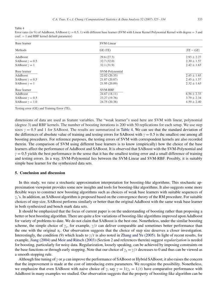
Table 4Error rates (in %) of AdaBoost, SABoost (�= 0.5, 1) with different base learner (SVM with Linear Kernel Polynomial Kernel with degree = 3 andcoef. = 1 and RBF kernel default parameter)
Base learner SVM-Linear
Methods GE (TE) |TE− GE|AdaBoost 29.6 (27.3) 2.93± 2.27SABoost �= 0.5 32.7 (32.0) 2.30± 1.57SABoost �= 1 32.1 (31.9) 2.42± 1.63
Base learner SVM-PolynomialAdaBoost 22.02 (20.35) 2.45± 1.65SABoost �= 0.5 21.87 (20.87) 2.45± 1.57SABoost �= 1 21.95 (20.89) 2.32± 1.63
Base learner SVM-RBFAdaBoost 24.67 (18.11) 6.56± 2.33SABoost �= 0.5 23.27 (19.76) 3.79± 2.34SABoost �= 1.0 24.75 (20.38) 4.59± 2.40
Testing error (GE) and Training Error (TE).
dimensions of data are used as feature variables. The “weak learner”s used here are SVM with linear, polynomial(degree 3) and RBF kernels. The number of boosting iterations is 200 with 50 replications for each setup. We use stepsizes � = 0.5 and 1 for SABoost. The results are summarized in Table 4. We can see that the standard deviation ofthe differences of absolute value of training and testing errors for SABoost with �= 0.5 is the smallest one among allboosting procedures. For reference purposes, the testing errors of SVM with correspondent kernels are also recordedtherein. The comparison of SVM using different base learners is to know (empirically) how the choice of the baselearners affect the performance of AdaBoost and SABoost. It is observed that SABoost with the SVM-Polynomial and�= 0.5 yields the best performance in the sense that it has the smallest testing error and a small difference of trainingand testing errors. In a way, SVM-Polynomial lies between the SVM-Linear and SVM-RBF. Possibly, it is suitablysimple base learner for the synthesized data sets.
5. Conclusion and discussion
In this study, we raise a stochastic approximation interpretation for boosting-like algorithms. This stochastic ap-proximation viewpoint provides some new insights and tools for boosting-like algorithms. It also suggests some moreflexible ways to construct new boosting algorithms such as choices of weak base learners with suitable sequences of�t ’s. In addition, an SABoost algorithm is proposed based on the convergence theory of the RM procedure. For suitablechoices of step size, SABoost performs similarly or better than the original AdaBoost with the same weak base learnerin both synthesized and bench mark data sets.
It should be emphasized that the focus of current paper is on the understanding of boosting rather than proposing abetter or best boosting algorithm. There are quite a few variations of boosting-like algorithms improved upon AdaBoostfor variety of problems to date. We do not claim that SABoost is the best one. Nonetheless, under the similar boostingscheme, the simple choice of �t , for example, �/t can deliver comparable and sometimes better performance thanthe one with the original �t . Our observation suggests that the choice of step size deserves a closer investigation.Interestingly, the condition (9) which leads to �/t is also noted in Zhang and Yu (2005). In light of recent results, forexample, Jiang (2004) and Meir and Rätsch (2003) (Section 2 and references therein) suggest regularization is neededfor boosting, particularly for noisy data. Regularization, loosely speaking, can be achieved by imposing constraints onthe base functions or through early stopping. Note that our choice of �t = �/t decreases to 0 and thus can be viewed asa smooth stopping rule.
Although fine tuning of � or can improve the performance of SABoost or Hybrid SABoost, it also raises the concernthat the improvement is made at the cost of introducing extra parameters. We recognize the possibility. Nonetheless,we emphasize that even SABoost with naive choice of �, say � = 1(�t = 1/t) have comparative performance withAdaBoost in many examples we studied. Our observation suggests that the property of boosting-like algorithm can be
334 C.A. Tsao, Y.-c.I. Chang / Computational Statistics & Data Analysis 52 (2007) 325–334
investigated under a simpler, data-independent �t contrasting to the original �t . Our experiments with Hybrid SABoostreveal that the step sizes in early stage of boosting can greatly affect the performances of boosting. Therefore, theboosting iterations should be understood at least from two parts: the early iterations which determines large part ofthe reduction of TE and GE; the latter iterations should be suitably regularized or early stopped preventing overfitting.Two ensuing questions are under current investigation.
1. How to choose a good �t for SABoost for a given base learner (with some distribution information of the data)?2. What base learners will produce �t in AdaBoost which are essentially equivalent to �t in SABoost (in terms of the
convergence rate of step size)?In addition, the stochastic versions and the KW parallels will be investigated in another paper.
Acknowledgments
The research is supported by NSC-95-2118-M-259-002-MY2, Taiwan. We would also like to thank Lin, Sung-Chiangfor his assistance in numerical computation and simulation.
References
Blake, C., Merz, C., 1998. UCI repository of machine learning databases.Breiman, L., 1999. Predicting games and arcing algorithms. Neural Comput. 11, 1493–1518.Breiman, L., 2004. Population theory for boosting ensembles. Ann. Statist. 32, 1–11.Bühlmann, P., Yu, B., 2003. Boosting with the l2-loss: regression and classification J. Amer. Statist. Assoc. 98 324–339.Duflo, M., 1997. Random iterative models. Series in Applications of Mathematics. Springer, New York.Freund, Y., Schapire, R., 1997. A decision-theoretic generalization of on-line learning and an application to boosting. J. of Comput. System Sci. 55,
119–139.Friedman, J., 2001. Greedy function approximation: a gradient boosting machine. Ann. Statist. 29, 1189–1232.Friedman, J., 2002. Stochastic gradient boosting. Comput. Statist. Data Anal. 38, 367–378.Friedman, J., Hastie, T., Tibishirani, R., 2000. Additive logistic regression: a statistical view of boosting (with discussion). Ann. of Statist. 28,
337–407.Gey, S., Poggi, J.-M., 2006. Boosting and instability for regression trees Comput. Statist. Data Anal. 50, 533–550.Grove, A., Schuurmans, D., 1998. Boosting in the limit: maximizing the margin of learned ensembles. in: Proceedings of the Fifteenth National
Conference on Artificial Intelligence. Madison, Wisconsin.Jiang, W., 2002. On weak base hypotheses and their implications for boosting regression and classification. Ann. Statist. 30, 51–73.Jiang, W., 2004. Process consistency for AdaBoost. Ann. Statist. 32, 13–29.Kiefer, J., Wolfowitz, J., 1952. Stochastic estimation of the maximum of a regression function. Ann. Math. Statist. 23, 462–466.Kim, Y., Koo, J.-Y., 2005. Inverse boosting for monotone regression functions. Comput. Statist. Data Anal. 49, 757–770.Kim, Y., Koo, J.-Y., 2006. Erratum to “Inverse boosting for monotone regression functions” Comput. Statist. Data Anal. 50, 583(Comput. Statist.
Data Anal. 49 (2005) 757–770).Lai, T.Z., 2003. Stochastic approximation: invited paper. Ann. Statist. 31, 391–406.Leitenstorfer, F., Tutz, G., 2007. Knot selection by boosting techniques. Comput. Statist. Data Anal. 51, 4605–4621.Meir, R., Rätsch, G., 2003.An introduction to boosting and leveraging. In: Mendelson, S., Smola,A. (Eds.),Advanced Lectures on Machine Learning.
Springer, New York, pp. 118–183.Merler, S., Caprile, B., Furlanello, C., 2007. Parallelizing AdaBoost by weights dynamics. Comput. Statist. Data Anal. 51, 2487–2498.Mika, S., Rätsch, G., Weston, J., Schölkopf, B., Müller, K.-R., 1999. Fisher discriminant analysis with kernels. Neural Networks for Signal Processing,
vol. IX. IEEE, New York, pp. 41–48.Rätsch, G., Onoda, T., Müller, K.-R., 2001. Soft margins for AdaBoost. Machine Learning, 42, 287–320. Also NeuroCOLT Technical Report
NC-TR-1998-021.Robbins, H., Monro, S., 1951. A stochastic approximation method. Ann. Math. Statist. 22, 400–407.Schapire, R., 1990. The strength of weak learnability. Mach. Learning 5, 197–227.Schapire, R., Freund, Y., Bartlett, P., Lee, W., 1998. Boosting the margin: a new explanation for the effectiveness of voting methods. Ann. Statist.
26, 1651–1686.Tutz, G., Binder, H., 2006. Boosting ridge regression. Computational Statistics and Data Analysis. Corrected Proof, Available online 22 December
2006, in press.Verzani, J., 2005. Using R for Introductory Statistics. Chapman & Hall, CRC Press, London, Boca Raton, FL. ISBN 1-584-88450-9.Zhang, T., Yu, B., 2005. Boosting with early stopping: convergence and consistency. Ann. Statist. 33, 1538–1579.


![Stochastic Successive Convex Approximation for …arXiv:1908.11015v1 [cs.IT] 29 Aug 2019 Stochastic Successive Convex Approximation for General Stochastic Optimization Problems with](https://img.pdfslide.us/doc/110x75/5f41e34ca12ac52e26340b0b/stochastic-successive-convex-approximation-for-arxiv190811015v1-csit-29-aug.jpg)


