Embed Size (px)
Citation preview
24
A Stepwise Auto-Profiling Method for Performance
Optimization of Streaming Applications
XUNYUN LIU, University of Melbourne, Australia
AMIR VAHID DASTJERDI, PwC Australia, Australia
RODRIGO N. CALHEIROS, Western Sydney University, Australia
CHENHAO QU and RAJKUMAR BUYA, University of Melbourne, Australia
Data stream management systems (DSMSs) are scalable, highly available, and fault-tolerant systems that
aggregate and analyze real-time data in motion. To continuously perform analytics on the fly within the
stream, state-of-the-art DSMSs host streaming applications as a set of interconnected operators, with each
operator encapsulating the semantic of a specific operation. For parallel execution on a particular platform,
these operators need to be appropriately replicated in multiple instances that split and process the workload
simultaneously. Because the way operators are partitioned affects the resulting performance of streaming
applications, it is essential for DSMSs to have a method to compare different operators and make holistic
replication decisions to avoid performance bottlenecks and resource wastage. To this end, we propose a step-
wise profiling approach to optimize application performance on a given execution platform. It automatically
scales distributed computations over streams based on application features and processing power of pro-
visioned resources and builds the relationship between provisioned resources and application performance
metrics to evaluate the efficiency of the resulting configuration. Experimental results confirm that the pro-
posed approach successfully fulfills its goals with minimal profiling overhead.
CCS Concepts: • Information systems → Data streams; Stream management; Database performance
evaluation; • Social and professional topics → Quality assurance; • Software and its engineering →
Software performance;
Additional Key Words and Phrases: Stream processing, data stream management systems, performance
optimization, resource management
ACM Reference format:
Xunyun Liu, Amir Vahid Dastjerdi, Rodrigo N. Calheiros, Chenhao Qu, and Rajkumar Buyya. 2017. A Stepwise
Auto-Profiling Method for Performance Optimization of Streaming Applications. ACM Trans. Auton. Adapt.
Syst. 12, 4, Article 24 (November 2017), 33 pages.
https://doi.org/10.1145/3132618
1 INTRODUCTION
Stream processing—a paradigm that supports leveraging data in motion for analytics—is rapidlyemerging due to continuous generation of data and the need for their timely processing. Usu-ally, stream processing is realized by a data stream management system (DSMS), a platform that
Authors’ addresses: X. Liu, C. Qu, and R. Buyya, Cloud Computing and Distributed Systems (CLOUDS) Lab, School of Com-
puting and Information Systems, The University of Melbourne, Australia; emails: {xunyunl, cqu}@student.unimelb.edu.au,
[email protected]; A. V. Dastjerdi, 2 Riverside Quay, Southbank VIC 3006; email: [email protected]; R. N.
Calheiros, Locked Bag 1797 Penrith NSW 2751 Australia; email: [email protected].
Permission to make digital or hard copies of all or part of this work for personal or classroom use is granted without fee
provided that copies are not made or distributed for profit or commercial advantage and that copies bear this notice and the
full citation on the first page. Copyrights for components of this work owned by others than the ACM must be honored.
Abstracting with credit is permitted. To copy otherwise, or republish, to post on servers or to redistribute to lists, requires
prior specific permission and/or a fee. Request permissions from [email protected].
© 2017 ACM 1556-4665/2017/11-ART24 $15.00
https://doi.org/10.1145/3132618
ACM Transactions on Autonomous and Adaptive Systems, Vol. 12, No. 4, Article 24. Publication date: November 2017.
24:2 X. Liu et al.
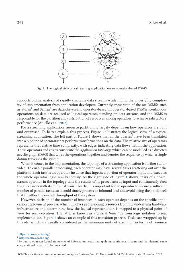
Fig. 1. The logical view of a streaming application on an operator-based DSMS.
supports online analysis of rapidly changing data streams while hiding the underlying complex-ity of implementation from application developers. Currently, most state-of-the-art DSMSs suchas Storm1 and Samza2 are data-driven and operator-based. In operator-based DSMSs, continuousoperations on data are realized as logical operators standing on data streams, and the DSMS isresponsible for the partition and distribution of resources among operators to achieve satisfactoryperformance (Aniello et al. 2013).
For a streaming application, resource partitioning largely depends on how operators are builtand organised. To better explain this process, Figure 1 illustrates the logical view of a typicalstreaming application. The left part of Figure 1 shows that all the queries3 have been translatedinto a pipeline of operators that perform transformations on the data. The relative size of operatorsrepresents the relative time complexity, with edges indicating data flows within the application.These operators and edges constitute the application topology, which can be modelled as a directedacyclic graph (DAG) that wires the operations together and denotes the sequence by which a singledatum traverses the system.
When it comes to the implementation, the topology of a streaming application is further subdi-vided. To enable parallel processing, each operator may have several tasks scattering out over theplatform. Each task is an operator instance that ingests a portion of operator input and executesthe whole operator logic simultaneously. As the right side of Figure 1 shows, tasks of a down-stream operator in the topology take the results of its precedents as input and continuously feedthe successors with its output stream. Clearly, it is important for an operator to secure a sufficientnumber of parallel tasks, so it could timely process its inbound load and avoid being the bottleneckthat throttles the overall throughput of the system.
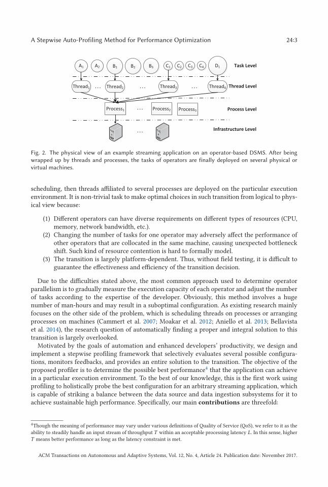
However, decision of the number of instances in each operator depends on the specific appli-cation deployment process, which involves provisioning resources from the underlying hardwareinfrastructure and determining how the logical representation is mapped to a physical point ofview for real execution. The latter is known as a critical transition from logic notation to realimplementation. Figure 2 shows an example of this transition process. Tasks are wrapped up bythreads, which are usually considered as the minimum units of execution in terms of resource
1https://storm.apache.org/.2 http://samza.apache.org.3By query, we mean formal statements of information needs that apply on continuous streams and that demand some
computational capacity to be processed.
ACM Transactions on Autonomous and Adaptive Systems, Vol. 12, No. 4, Article 24. Publication date: November 2017.
A Stepwise Auto-Profiling Method for Performance Optimization 24:3
Fig. 2. The physical view of an example streaming application on an operator-based DSMS. After being
wrapped up by threads and processes, the tasks of operators are finally deployed on several physical or
virtual machines.
scheduling, then threads affiliated to several processes are deployed on the particular executionenvironment. It is non-trivial task to make optimal choices in such transition from logical to phys-ical view because:
(1) Different operators can have diverse requirements on different types of resources (CPU,memory, network bandwidth, etc.).
(2) Changing the number of tasks for one operator may adversely affect the performance ofother operators that are collocated in the same machine, causing unexpected bottleneckshift. Such kind of resource contention is hard to formally model.
(3) The transition is largely platform-dependent. Thus, without field testing, it is difficult toguarantee the effectiveness and efficiency of the transition decision.
Due to the difficulties stated above, the most common approach used to determine operatorparallelism is to gradually measure the execution capacity of each operator and adjust the numberof tasks according to the expertise of the developer. Obviously, this method involves a hugenumber of man-hours and may result in a suboptimal configuration. As existing research mainlyfocuses on the other side of the problem, which is scheduling threads on processes or arrangingprocesses on machines (Cammert et al. 2007; Moakar et al. 2012; Aniello et al. 2013; Bellavistaet al. 2014), the research question of automatically finding a proper and integral solution to thistransition is largely overlooked.
Motivated by the goals of automation and enhanced developers’ productivity, we design andimplement a stepwise profiling framework that selectively evaluates several possible configura-tions, monitors feedbacks, and provides an entire solution to the transition. The objective of theproposed profiler is to determine the possible best performance4 that the application can achievein a particular execution environment. To the best of our knowledge, this is the first work usingprofiling to holistically probe the best configuration for an arbitrary streaming application, whichis capable of striking a balance between the data source and data ingestion subsystems for it toachieve sustainable high performance. Specifically, our main contributions are threefold:
4Though the meaning of performance may vary under various definitions of Quality of Service (QoS), we refer to it as the
ability to steadily handle an input stream of throughput T within an acceptable processing latency L. In this sense, higher
T means better performance as long as the latency constraint is met.
ACM Transactions on Autonomous and Adaptive Systems, Vol. 12, No. 4, Article 24. Publication date: November 2017.
24:4 X. Liu et al.
—Our profiling system automatically scales up the streaming application on a given platform.Such processing parallelization is achieved by profiling of both application features andprocessing power of provisioned resources. Therefore, developers are no longer required toprovide parallel settings beforehand.
—The profiling strategy is designed as a feedback control loop that allows for self-adaptivity,scalability, and general applicability to a wide range of streaming applications, which isdemonstrated in our experiments.
—Based on the result of profiling, the relationship between resource provisioning and per-formance metrics of application is built, enabling further evaluation of the efficiencies ofcandidate topologies that are implemented for the same streaming application.
2 MOTIVATION
The development cycle of a streaming application on an operator-based DSMS typically consists oftwo phases. The first phase consists in the logic development, where all the continuous queries orother data operations are implemented as logical operators working on data streams. The secondphase consists in the application deployment, which mainly comprises a transition from logicalto physical view. In this phase, the parallelism setting for each operator is determined and thedecision on how tasks of operators are wrapped up and mapped to underlying resources is made,which are collectively referred to as a parallel configuration. Our primary motivation is to automatethe transition and ensure that, in the resulting configuration, resources are properly partitionedamong operators to enable better performance.
As mentioned above, optimization of the application deployment is a nontrivial process. Hereare three fundamental prerequisites that a streaming application should meet before it comes intoservice.
Application scaling: Scaling up5 is a critical process for a streaming application to use dis-tributed resources. As scaling is both resource specific and topology dependent, there is no uni-versal model able to provide a general solution. Therefore, the transition in the second phase has tobe designed and performed by developers according to their own experiences, which causes addi-tional development burden and may not yield efficient resource utilization. It becomes even moreproblematic when the underlying resource structure is configurable. State-of-the-art DSMSs areintegrating elasticity into their implementation to enable resource consumptions customizationwith regard to fluctuating workloads. They support (1) dynamic resizing, for example, DSMS canbe scaled out by adding new machines, and (2) adjustable operator parallelization, which allowsstateful and stateless operators to choose their number of tasks to suit different sizes of executionenvironment. However, applications running on an elastic DSMS do not have the ability to adapttheir configuration to infrastructure changes, meaning that they are unable to automatically takeadvantage of newly added compute resources when the DSMS is scaled out, and may face severeresource contention due to excessive parallelization when the DSMS is scaled in. Our work fillsin this gap by automating the scaling-up process once the underlying system is updated, whichcomplements efforts toward making DSMS scalable and elastic (Schneider et al. 2009, 2012; CastroFernandez et al. 2013; Gedik et al. 2014).
Besides, it is also desirable to quantitatively evaluate how efficient the transition is and au-tomatically probe whether there is still room for improvements. However, due to the labor-intensive task of manual deployment, it is a common practice for developers to stop scaling up the
5Scaling up refers to further parallelizing the execution of logical operators to improve the resource utilization of a stream-
ing application, whereas scaling out/in stands for adding or removing machines.
ACM Transactions on Autonomous and Adaptive Systems, Vol. 12, No. 4, Article 24. Publication date: November 2017.
A Stepwise Auto-Profiling Method for Performance Optimization 24:5
application when a transition that meets the requirement of performance is found. Nevertheless,it may result in suboptimal resource utilization.
DAGs comparison: The topology of a streaming application is organised as a directed acyclicgraph (DAG) of logical operators. However, the conversion of queries and operations on datastreams into operators, which is performed in the first phase, can be conducted in multiple ways,resulting in different topologies that are logically equivalent. It means that, although differenttypes of DAGs are formed by operators, they take the same input stream and all produce correctanswers. It is difficult but still necessary to determine which one is better with respect to theirperformances in a particular platform.
Resource requirement analysis: It is essential to know how many resources are needed tomeet time constraints to handle the inbound stream. The answer depends on the volume of theinput stream and the application resource needs per input data element. In the context of streamprocessing, the input stream may vary significantly in volume and speed and so does the amountof resource needed per element. Usually, application developers do not have control over the inputdata (Hummer et al. 2013), but tracking the latter could help them to guarantee real-time responsewith minimal resource consumption when the workload varies. Based on this, a rule-based auto-scaling approach could be proposed.
In this article, we choose application profiling as an empirical and adaptive approach to fulfillthe above targets. Compared to analytical models based on abstract modelling, profiling excels as itprovides more reliable results via real experiments. Furthermore, by taking advantage of profiling,our method is generic enough to support different execution environments, including variationsin characteristics of underlying resources, load balancing of DSMS, and the type of streamingapplication running on it. Besides, a recalibration mechanism has been introduced to ensure thatthe decision on parallel configuration is up-to-date. Therefore, possible changes to application andDSMS, as well as data-dependent variation affecting the execution time of data elements, will notcompromise the accuracy of profiled knowledge.
3 STEPWISE PROFILING OVERVIEW
The profiling process works by selectively evaluating several possible configurations and finallychoosing the one that shows the most promising performance potential, that is, the one capableof processing more data streams per unit time while meeting the latency requirement.
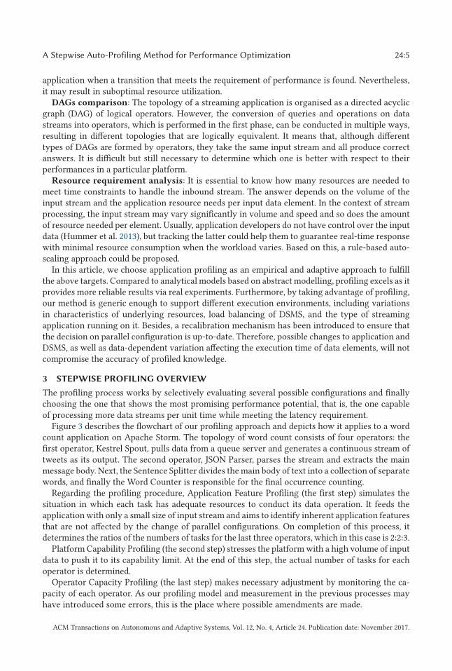
Figure 3 describes the flowchart of our profiling approach and depicts how it applies to a wordcount application on Apache Storm. The topology of word count consists of four operators: thefirst operator, Kestrel Spout, pulls data from a queue server and generates a continuous stream oftweets as its output. The second operator, JSON Parser, parses the stream and extracts the mainmessage body. Next, the Sentence Splitter divides the main body of text into a collection of separatewords, and finally the Word Counter is responsible for the final occurrence counting.
Regarding the profiling procedure, Application Feature Profiling (the first step) simulates thesituation in which each task has adequate resources to conduct its data operation. It feeds theapplication with only a small size of input stream and aims to identify inherent application featuresthat are not affected by the change of parallel configurations. On completion of this process, itdetermines the ratios of the numbers of tasks for the last three operators, which in this case is 2:2:3.
Platform Capability Profiling (the second step) stresses the platform with a high volume of inputdata to push it to its capability limit. At the end of this step, the actual number of tasks for eachoperator is determined.
Operator Capacity Profiling (the last step) makes necessary adjustment by monitoring the ca-pacity of each operator. As our profiling model and measurement in the previous processes mayhave introduced some errors, this is the place where possible amendments are made.
ACM Transactions on Autonomous and Adaptive Systems, Vol. 12, No. 4, Article 24. Publication date: November 2017.
24:6 X. Liu et al.
Fig. 3. Flowchart of stepwise profiling and a working demonstration on a word count application.
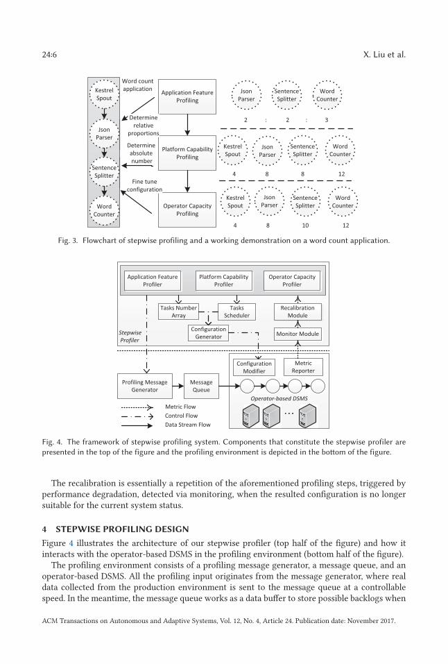
Fig. 4. The framework of stepwise profiling system. Components that constitute the stepwise profiler are
presented in the top of the figure and the profiling environment is depicted in the bottom of the figure.
The recalibration is essentially a repetition of the aforementioned profiling steps, triggered byperformance degradation, detected via monitoring, when the resulted configuration is no longersuitable for the current system status.
4 STEPWISE PROFILING DESIGN
Figure 4 illustrates the architecture of our stepwise profiler (top half of the figure) and how itinteracts with the operator-based DSMS in the profiling environment (bottom half of the figure).
The profiling environment consists of a profiling message generator, a message queue, and anoperator-based DSMS. All the profiling input originates from the message generator, where realdata collected from the production environment is sent to the message queue at a controllablespeed. In the meantime, the message queue works as a data buffer to store possible backlogs when
ACM Transactions on Autonomous and Adaptive Systems, Vol. 12, No. 4, Article 24. Publication date: November 2017.
A Stepwise Auto-Profiling Method for Performance Optimization 24:7
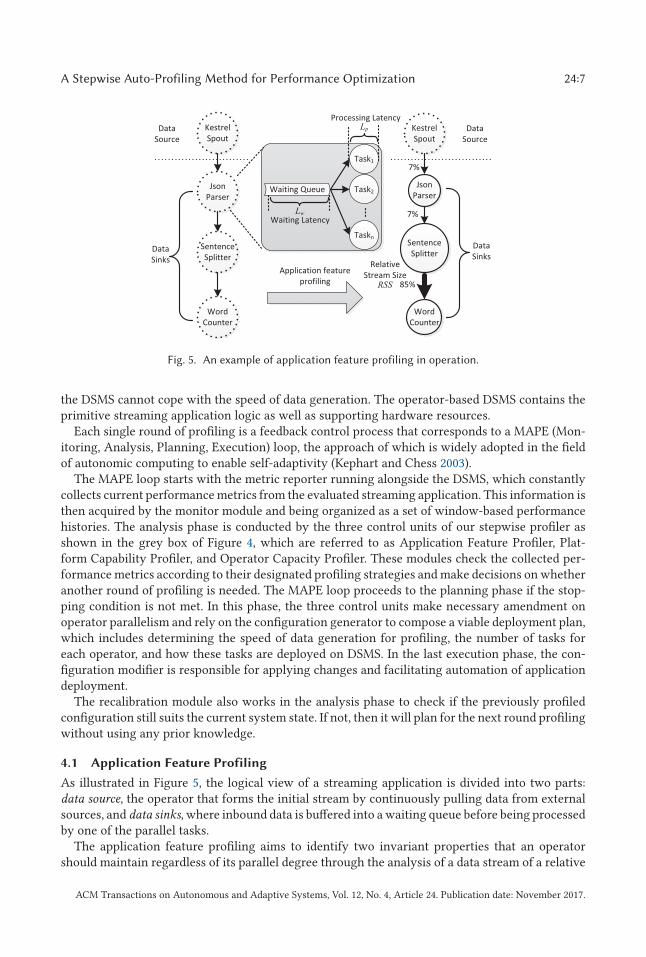
Fig. 5. An example of application feature profiling in operation.
the DSMS cannot cope with the speed of data generation. The operator-based DSMS contains theprimitive streaming application logic as well as supporting hardware resources.
Each single round of profiling is a feedback control process that corresponds to a MAPE (Mon-itoring, Analysis, Planning, Execution) loop, the approach of which is widely adopted in the fieldof autonomic computing to enable self-adaptivity (Kephart and Chess 2003).
The MAPE loop starts with the metric reporter running alongside the DSMS, which constantlycollects current performance metrics from the evaluated streaming application. This information isthen acquired by the monitor module and being organized as a set of window-based performancehistories. The analysis phase is conducted by the three control units of our stepwise profiler asshown in the grey box of Figure 4, which are referred to as Application Feature Profiler, Plat-form Capability Profiler, and Operator Capacity Profiler. These modules check the collected per-formance metrics according to their designated profiling strategies and make decisions on whetheranother round of profiling is needed. The MAPE loop proceeds to the planning phase if the stop-ping condition is not met. In this phase, the three control units make necessary amendment onoperator parallelism and rely on the configuration generator to compose a viable deployment plan,which includes determining the speed of data generation for profiling, the number of tasks foreach operator, and how these tasks are deployed on DSMS. In the last execution phase, the con-figuration modifier is responsible for applying changes and facilitating automation of applicationdeployment.
The recalibration module also works in the analysis phase to check if the previously profiledconfiguration still suits the current system state. If not, then it will plan for the next round profilingwithout using any prior knowledge.
4.1 Application Feature Profiling
As illustrated in Figure 5, the logical view of a streaming application is divided into two parts:data source, the operator that forms the initial stream by continuously pulling data from externalsources, and data sinks, where inbound data is buffered into a waiting queue before being processedby one of the parallel tasks.
The application feature profiling aims to identify two invariant properties that an operatorshould maintain regardless of its parallel degree through the analysis of a data stream of a relative
ACM Transactions on Autonomous and Adaptive Systems, Vol. 12, No. 4, Article 24. Publication date: November 2017.
24:8 X. Liu et al.
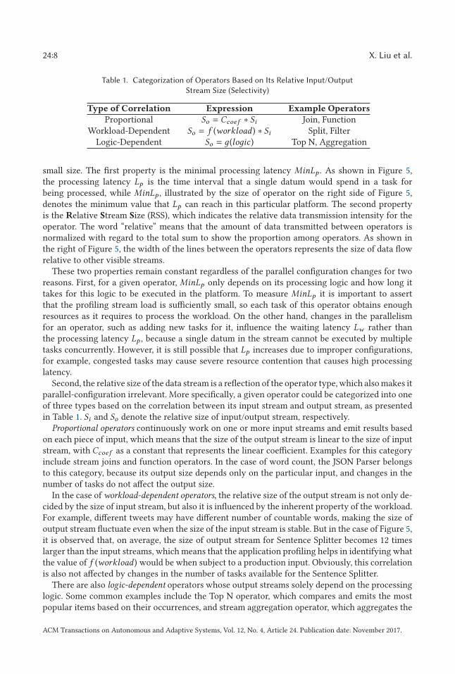
Table 1. Categorization of Operators Based on Its Relative Input/Output
Stream Size (Selectivity)
Type of Correlation Expression Example Operators
Proportional So = Ccoef ∗ Si Join, FunctionWorkload-Dependent So = f (workload ) ∗ Si Split, Filter
Logic-Dependent So = д(loдic ) Top N, Aggregation
small size. The first property is the minimal processing latency MinLp . As shown in Figure 5,the processing latency Lp is the time interval that a single datum would spend in a task forbeing processed, while MinLp , illustrated by the size of operator on the right side of Figure 5,denotes the minimum value that Lp can reach in this particular platform. The second propertyis the Relative Stream Size (RSS), which indicates the relative data transmission intensity for theoperator. The word “relative” means that the amount of data transmitted between operators isnormalized with regard to the total sum to show the proportion among operators. As shown inthe right of Figure 5, the width of the lines between the operators represents the size of data flowrelative to other visible streams.
These two properties remain constant regardless of the parallel configuration changes for tworeasons. First, for a given operator, MinLp only depends on its processing logic and how long ittakes for this logic to be executed in the platform. To measure MinLp it is important to assertthat the profiling stream load is sufficiently small, so each task of this operator obtains enoughresources as it requires to process the workload. On the other hand, changes in the parallelismfor an operator, such as adding new tasks for it, influence the waiting latency Lw rather thanthe processing latency Lp , because a single datum in the stream cannot be executed by multipletasks concurrently. However, it is still possible that Lp increases due to improper configurations,for example, congested tasks may cause severe resource contention that causes high processinglatency.
Second, the relative size of the data stream is a reflection of the operator type, which also makes itparallel-configuration irrelevant. More specifically, a given operator could be categorized into oneof three types based on the correlation between its input stream and output stream, as presentedin Table 1. Si and So denote the relative size of input/output stream, respectively.
Proportional operators continuously work on one or more input streams and emit results basedon each piece of input, which means that the size of the output stream is linear to the size of inputstream, with Ccoef as a constant that represents the linear coefficient. Examples for this categoryinclude stream joins and function operators. In the case of word count, the JSON Parser belongsto this category, because its output size depends only on the particular input, and changes in thenumber of tasks do not affect the output size.
In the case of workload-dependent operators, the relative size of the output stream is not only de-cided by the size of input stream, but also it is influenced by the inherent property of the workload.For example, different tweets may have different number of countable words, making the size ofoutput stream fluctuate even when the size of the input stream is stable. But in the case of Figure 5,it is observed that, on average, the size of output stream for Sentence Splitter becomes 12 timeslarger than the input streams, which means that the application profiling helps in identifying whatthe value of f (workload ) would be when subject to a production input. Obviously, this correlationis also not affected by changes in the number of tasks available for the Sentence Splitter.
There are also logic-dependent operators whose output streams solely depend on the processinglogic. Some common examples include the Top N operator, which compares and emits the mostpopular items based on their occurrences, and stream aggregation operator, which aggregates the
ACM Transactions on Autonomous and Adaptive Systems, Vol. 12, No. 4, Article 24. Publication date: November 2017.
A Stepwise Auto-Profiling Method for Performance Optimization 24:9
input stream or regularly performs batch operations. The Word Counter operator in Figure 5 isused for aggregation and thus is an example of a logic-dependent operator.
Whenever an operator becomes a bottleneck, the DSMS has to throttle the upstream and down-stream operators to maintain the system stability. This leads to the observation that the streamingapplication can be well-approximated with an intuitive queueing network of data flow, which runson a computational system of unknown capability where contention affects all tasks in the sameway. The latter assumption may not always hold true during the runtime, but it is reasonable forus to depict the relative parallelism requirement for each operator.
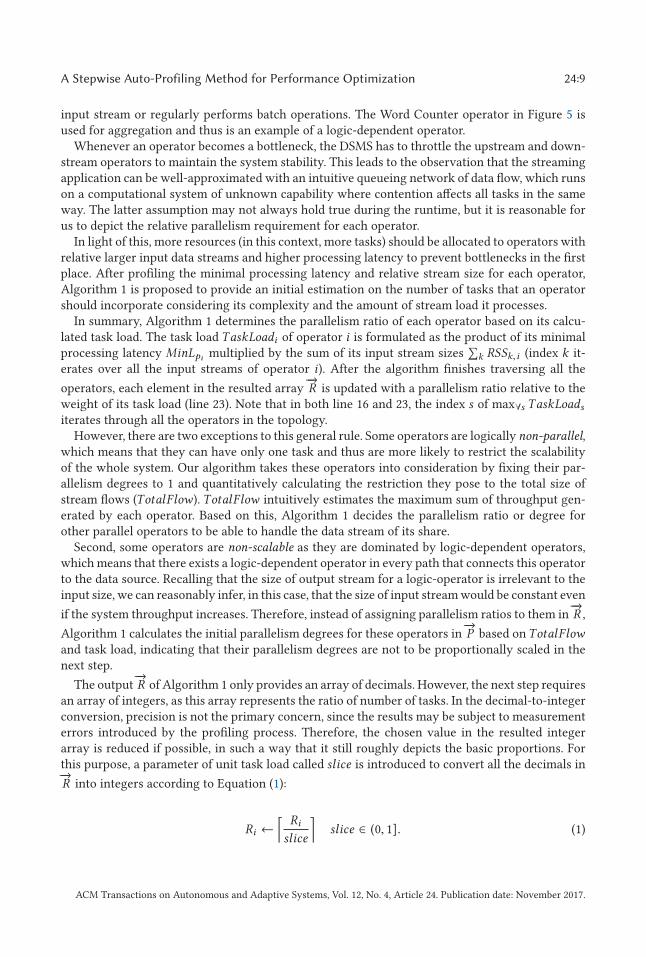
In light of this, more resources (in this context, more tasks) should be allocated to operators withrelative larger input data streams and higher processing latency to prevent bottlenecks in the firstplace. After profiling the minimal processing latency and relative stream size for each operator,Algorithm 1 is proposed to provide an initial estimation on the number of tasks that an operatorshould incorporate considering its complexity and the amount of stream load it processes.
In summary, Algorithm 1 determines the parallelism ratio of each operator based on its calcu-lated task load. The task load TaskLoadi of operator i is formulated as the product of its minimalprocessing latency MinLpi
multiplied by the sum of its input stream sizes∑
k RSSk,i (index k it-erates over all the input streams of operator i). After the algorithm finishes traversing all the
operators, each element in the resulted array−→R is updated with a parallelism ratio relative to the
weight of its task load (line 23). Note that in both line 16 and 23, the index s of max∀s TaskLoads
iterates through all the operators in the topology.However, there are two exceptions to this general rule. Some operators are logically non-parallel,
which means that they can have only one task and thus are more likely to restrict the scalabilityof the whole system. Our algorithm takes these operators into consideration by fixing their par-allelism degrees to 1 and quantitatively calculating the restriction they pose to the total size ofstream flows (TotalFlow). TotalFlow intuitively estimates the maximum sum of throughput gen-erated by each operator. Based on this, Algorithm 1 decides the parallelism ratio or degree forother parallel operators to be able to handle the data stream of its share.
Second, some operators are non-scalable as they are dominated by logic-dependent operators,which means that there exists a logic-dependent operator in every path that connects this operatorto the data source. Recalling that the size of output stream for a logic-operator is irrelevant to theinput size, we can reasonably infer, in this case, that the size of input stream would be constant even
if the system throughput increases. Therefore, instead of assigning parallelism ratios to them in−→R ,
Algorithm 1 calculates the initial parallelism degrees for these operators in−→P based onTotalFlow
and task load, indicating that their parallelism degrees are not to be proportionally scaled in thenext step.
The output−→R of Algorithm 1 only provides an array of decimals. However, the next step requires
an array of integers, as this array represents the ratio of number of tasks. In the decimal-to-integerconversion, precision is not the primary concern, since the results may be subject to measurementerrors introduced by the profiling process. Therefore, the chosen value in the resulted integerarray is reduced if possible, in such a way that it still roughly depicts the basic proportions. Forthis purpose, a parameter of unit task load called slice is introduced to convert all the decimals in−→R into integers according to Equation (1):
Ri ←⌈ Ri
slice
⌉slice ∈ (0, 1]. (1)
ACM Transactions on Autonomous and Adaptive Systems, Vol. 12, No. 4, Article 24. Publication date: November 2017.
24:10 X. Liu et al.
ALGORITHM 1: Calculate the Relative Ratio or Number of Tasks for Each Operator.
Input: MinLpi : minimum processing latency of operator iInput: RSSi, j : relative stream size between consecutive operators i and j
Output:−→R : parallelism ratio array of parallel operators, in which Ri corresponds to operator i
Output:−→P : parallelism degree array of non-parallel and non-scalable operators, in which Pj
corresponds to operator j
1 Initialize each element of−→R to 1;
2 TotalFlow ← ∞;
3 Identify all the operators that are dominated by logic-dependent operator, label them as Non-Scalable;
4 foreach Operator i do
5 if i is Non-Parallel then
6 Pi ← 1 ;
7 TotalFlow ← min(TotalFlow, 1MinLpi
∗∑k
RSSk,i);
8 end
9 else
/* Calculate TaskLoad for parallel operator i */
10 TaskLoadi ← MinLpi ∗∑
kRSSk,i ;
11 end
12 end
13 foreach Parallel Operator i do
14 if i is Non-Scalable then
15 if TotalFlow = ∞ then
16 Pi ← � T askLoadi
min∀s
T askLoads;
17 end
18 else
19 Pi ← �TaskLoadi ∗TotalFlow;20 end
21 end
22 else
23 Ri ← T askLoadi
max∀s
T askLoads;
24 end
25 end
26 return−→R ,−→P ;
The value of slice should be tailored to the specific streaming application. Our rule of thumb isto try small values (0.1, 0.2, etc.) and select the one that minimizes the profiling effort in the nextstep. Section 6.4 will shed more light on the parameter selection with real experiments.
It is also worth mentioning that in line 3, we omit the process of identifying dominance rela-tionship for the sake of simplicity. Actually, there are some breadth-first searches starting fromeach logic-dependent operator to examine which operators are affected logic-dependent succes-sors. In summary, the algorithm sequentially evaluates the operator located at the head of queuewith regard to the status of its predecessors (each operator maintains a HashSet of all its status-undetermined predecessors for quick location and removal). If an operator has all its predecessorsmarked as either logic-dependent or already dominated, that is, its HashSet of status-undetermined
ACM Transactions on Autonomous and Adaptive Systems, Vol. 12, No. 4, Article 24. Publication date: November 2017.
A Stepwise Auto-Profiling Method for Performance Optimization 24:11
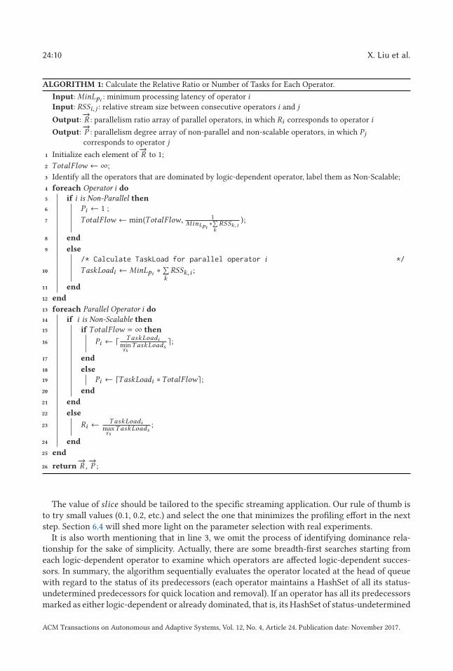
Fig. 6. An example of platform capability profiling in operation.
predecessors is emptied while this operator dequeues, then it then should be identified as domi-nated and its successors are added to the tail of queue for further evaluation.
Algorithm 1 also has a computational complexity of O (n) with the worst case being O (n ∗(d−avд + 2)), in which n is the number of operators and d−avд is the average vertex in-degree in thetopology graph. The most time-consuming step lies in line 3 as each operator in the topology maybe repeatedly visited, at most, its in-degree times to determine whether it has been dominated bylogic-dependent operators or not. Besides line 3, the algorithm body traverses the topology graphonly twice and all the required input can be collected with simply one round of profiling.
4.2 Platform Capability Profiling
Unlike the previous step, which requires only a small data stream to probe application features,the platform capability profiling requires the message generator to produce a continuous datastream that is large enough to stress the streaming application. Given sufficient profiling data, theconfiguration of the application is changed through a trial-and-error process to determine the realcapability of DSMS as well as its underlying infrastructure. The resulting configuration reveals areasonable choice of resource partition in this platform where it is capable of handling a relativelylarge stream without violating the latency constraint.6
As shown in Figure 6, each configuration trial is first evaluated in terms of system performancevariation. Specifically, changes in throughput and latency are collected and reported to the monitormodule, which can be used to identify if the new configuration improves the resource utilization.Configuration changes that have a negative impact on the system performance are discarded inthis phase.
Based on the result of performance evaluation, the profiler applies changes to the configura-tion according to Algorithm 2 and generates a new one for the next round of profiling. The newconfiguration not only targets throughput improvement, but also aims at maintaining the balancebetween data source and data sinks. If it failed to do so, then an overly powerful data source may
6Different applications may have different preferences with regard to their desirable performance. Though the final decision
is left up to the application developer, as a default the profiler favours better throughput on the condition that the system
still meets the pre-defined latency requirement.
ACM Transactions on Autonomous and Adaptive Systems, Vol. 12, No. 4, Article 24. Publication date: November 2017.
24:12 X. Liu et al.
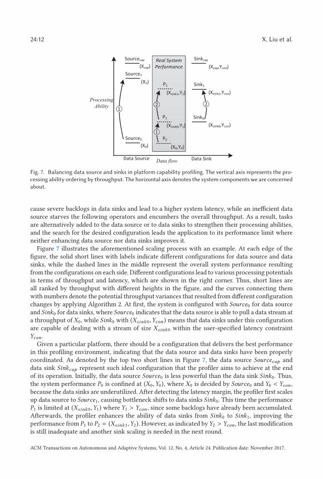
Fig. 7. Balancing data source and sinks in platform capability profiling. The vertical axis represents the pro-
cessing ability ordering by throughput. The horizontal axis denotes the system components we are concerned
about.
cause severe backlogs in data sinks and lead to a higher system latency, while an inefficient datasource starves the following operators and encumbers the overall throughput. As a result, tasksare alternatively added to the data source or to data sinks to strengthen their processing abilities,and the search for the desired configuration leads the application to its performance limit whereneither enhancing data source nor data sinks improves it.
Figure 7 illustrates the aforementioned scaling process with an example. At each edge of thefigure, the solid short lines with labels indicate different configurations for data source and datasinks, while the dashed lines in the middle represent the overall system performance resultingfrom the configurations on each side. Different configurations lead to various processing potentialsin terms of throughput and latency, which are shown in the right corner. Thus, short lines areall ranked by throughput with different heights in the figure, and the curves connecting themwith numbers denote the potential throughput variances that resulted from different configurationchanges by applying Algorithm 2. At first, the system is configured with Source0 for data sourceand Sink0 for data sinks, where Source0 indicates that the data source is able to pull a data stream ata throughput of X0, while Sink0 with (Xsink0,Ycon ) means that data sinks under this configurationare capable of dealing with a stream of size Xsink0 within the user-specified latency constraintYcon .
Given a particular platform, there should be a configuration that delivers the best performancein this profiling environment, indicating that the data source and data sinks have been properlycoordinated. As denoted by the top two short lines in Figure 7, the data source Sourcecap anddata sink Sinkcap represent such ideal configuration that the profiler aims to achieve at the endof its operation. Initially, the data source Source0 is less powerful than the data sink Sink0. Thus,the system performance P0 is confined at (X0,Y0), where X0 is decided by Source0 and Y0 < Ycon ,because the data sinks are underutilized. After detecting the latency margin, the profiler first scalesup data source to Source1, causing bottleneck shifts to data sinks Sink0. This time the performanceP1 is limited at (Xsink0,Y1) where Y1 > Ycon , since some backlogs have already been accumulated.Afterwards, the profiler enhances the ability of data sinks from Sink0 to Sink1, improving theperformance from P1 to P2 = (Xsink1,Y2). However, as indicated byY2 > Ycon , the last modificationis still inadequate and another sink scaling is needed in the next round.
ACM Transactions on Autonomous and Adaptive Systems, Vol. 12, No. 4, Article 24. Publication date: November 2017.
A Stepwise Auto-Profiling Method for Performance Optimization 24:13
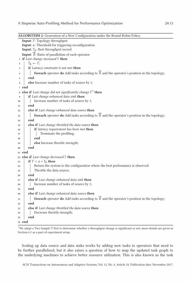
ALGORITHM 2: Generation of a New Configuration under the Round-Robin Policy.
Input: T : Topology throughput
Input: α : Threshold for triggering reconfiguration
Input: Tb : Best throughput record
Input:−→R : Ratio of parallelism of each operator
1 if Last change increased T then
2 Tb ← T ;
3 if Latency constraint is not met then
4 foreach operator do Add tasks according to−→R and the operator’s position in the topology;
5 end
6 else Increase number of tasks of source by 1;
7 end
8 else if Last change did not significantly change T † then
9 if Last change enhanced data sink then
10 Increase number of tasks of source by 1;
11 end
12 else if Last change enhanced data source then
13 foreach operator do Add tasks according to−→R and the operator’s position in the topology;
14 end
15 else if Last change throttled the data source then
16 if latency requirement has been met then
17 Terminate the profiling;
18 end
19 else Increase throttle strength;
20 end
21 end
22 else if Last change decreased T then
23 if T < α ∗Tb then
24 Return the system to the configuration where the best performance is observed;
25 Throttle the data source;
26 end
27 else if Last change enhanced data sink then
28 Increase number of tasks of source by 1;
29 end
30 else if Last change enhanced data source then
31 foreach operator do Add tasks according to−→R and the operator’s position in the topology;
32 end
33 else if Last change throttled the data source then
34 Decrease throttle strength;
35 end
36 end
†We adopt a Two Sample T-Test to determine whether a throughput change is significant or not; more details are given in
Section 6.1 as a part of experiment setup.
Scaling up data source and data sinks works by adding new tasks to operators that need tobe further parallelized, but it also raises a question of how to map the updated task graph tothe underlying machines to achieve better resource utilization. This is also known as the task
ACM Transactions on Autonomous and Adaptive Systems, Vol. 12, No. 4, Article 24. Publication date: November 2017.
24:14 X. Liu et al.
placement and scheduling problem. There are several policies available to decide the distributionof tasks across the platform, and certain applications may require a particular policy to suit a veryspecific need (e.g., assigning a particular task to a particular machine due to licence restrictions).We therefore design the platform capability profiler to enable scheduling policies to be pluggedin so it can be used in conjunction with various scheduling heuristics with different optimizationtargets, such as minimizing inter-node communication (Aniello et al. 2013; Xu et al. 2014), reducingthe average tuple processing time (Li et al. 2015), and being resource-aware to ensure the capabilityof each task to handle its task load (Peng et al. 2015). Since the focus of this work does not lie in taskplacement and scheduling, we introduce our profiling approach in tandem with the widely adoptedround-robin policy7 and apply it in a platform with homogeneous computational resources for easeof presentation. The round-robin policy is particularly suitable for homogeneous platforms as tasksare evenly distributed among available machines to enable fault-tolerance and load-balancing.
Algorithm 2 shows the interplay between performance evaluation and configuration generationcarried out by the profiler under the round-robin policy. Scaling data sources is a relatively light-weight operation: it only requires the number of tasks for the data source to be increased by 1, sothe application has one extra task pulling data from the message queue and thus increasing theinput rate. However, decision about increasing the parallelism for a data sink operator dependson the type of operator and its position in the topology. For example, an operator should keep itsnumber of tasks unchanged if it is a non-parallel operator, or if it is non-scalable dominated bylogic-dependent operators as its input stream tends to be steady during the profiling process. As
for other types of operators,−→R indicates the extent of enhancement for each operator.
Nevertheless, not every scaling effort, especially those applied for data sinks, can guaranteeimprovements. The reason why scaling data sinks is even more difficult than scaling data sourcesis that it has to exhaust current resources for additional computation and coordination. Therefore,to meet the latency constraint, our profiler performs a third operation on configuration, source
throttle, which limits the size of input stream by controlling the amount of data that is allowed tosojourn in the system.
The complexity of computation required for configuration generation is constant. However,the profiling process that evaluates the effectiveness of a new configuration is relatively time-consuming, since performance measurement must wait until the application is stabilized. To ex-amine the number of profiling rounds required in the worst case, we regard Algorithm 2 as asearch algorithm that explores a vectored value space, with each dimension confined by the actualparallelism degrees that can be seen in the ideal configuration. Given the fact that every three
consecutive profiling efforts can increase the total number of used tasks at least by ‖−→R ‖1 throughdata sink enhancement (except for consecutive source throttles, which is rare), and that assigningexcessive parallelism degree to an operator would harm the application performance, it is intu-
itive to deduce a conservative estimate that in the worst case there will be no more than 3 ∗ nMaxp
‖−→R ‖1rounds of profiling. In the expression, n is the number of operators in the topology, and Maxp
represents the maximal parallelism degree among all the operators. However, Maxp is unknownbefore the actual profiling, but it can be approximated in practice by the number of threads ableto run simultaneously in this particular platform (by multiplying the number of available cores bythe number of thread(s) per core).
7http://grokbase.com/t/gg/storm-user/132fh5qyve/recommendations-for-setting-num-isolated-machines-num-workers-
parallelism-hint.
ACM Transactions on Autonomous and Adaptive Systems, Vol. 12, No. 4, Article 24. Publication date: November 2017.
A Stepwise Auto-Profiling Method for Performance Optimization 24:15
4.3 Operator Capacity Profiling
The previous step of profiling divided the streaming application into two parts (data sources andsinks), of which the parallel configurations of operators are collectively adjusted based on the over-all performance of the system. Such coarse modifications may not be accurate enough to achievethe targeted configuration. Therefore, in the third step, profiling is carried out at operator levelthrough the individual evaluation of performance of each operator. The goal of this step is toachieve finer granularity of performance tuning.
Operator capacity, which is formally defined in Equation (2), is used to quantitatively evaluatethe degree of utilization of operators in data sinks. In the equation,Operator_latency is the averagetime that a single datum would spend in this operator over a specific time period. The length ofsuch time period is calledWindow_size and the amount of data processed in this period is denotedby Executed_load . Thus, capacity represents the percentage of the time in the observation timewindow that the operator spent executing inputs. The closer to 1 this value is, the more likely theoperator is the bottleneck in our topology:
Capacity =Operator_latency ∗ Executed_load
W indow_size. (2)
This step utilizes the same profiling environment used in the previous step. However, besidesoverall performance metrics such as throughput and latency, the profiler in this stage also collectsthe capacity information from each operator for fine-grained evaluation. The profiling strategyalso resembles the previous one: the performance evaluation phase sheds light on the system sta-tus and the possible bottleneck, and the previous configuration change is revoked if it causes per-formance degradation. However, this process differs from the previous step in that it has only oneoperation, which is increasing the number of tasks by 1 for the operator that has the highest capac-ity and has not been enhanced nor revoked. If there is no performance improvement obtained fromenhancing the operator with the highest capacity, then the operator that has the second-highestcapacity is tested in the next round and so on.
There are two stopping conditions for the profiling. The first is when there are consecutiverevocations observed, indicating that recent scaling-up efforts on candidate operators have failed.The second condition is when all the measured operator latencies approach the minimal processinglatency MinLp by a factor k . We evaluate the effect of diverse values of k in the performance ofthe profiling later in Section 6.4.
4.4 Recalibration Mechanism
The application of the above three profiling steps yields a specific parallel configuration that buildsa relation between provisioned resources and performance metrics. However, such relation is per-ceived to be volatile, since the performance under the same configuration may vary and the re-sulting configuration may need to be promptly modified due to the live changes that happen tothe streaming application or platform. This section therefore discusses the recalibration mecha-nism, which repeats the profiling process when necessary to keep the configuration and operatorprofiling up-to-date with minimal adjustment cost.
In general, recalibration is triggered by any three types of changes: (i) resizing of DSMS, whichleads to a new platform to be profiled after the infrastructure layer is dynamically scaled; (ii)re-deployment of the application, resulting from the alteration of application topology and themanipulation of some critical parameters that would greatly affect the application behaviour; and(iii) data-dependent variation, an uncontrollable factor related to the characteristic of workload,causing performance to vary even if the configuration remains unchanged.
ACM Transactions on Autonomous and Adaptive Systems, Vol. 12, No. 4, Article 24. Publication date: November 2017.
24:16 X. Liu et al.
For the first two causes, the recalibration decision is straightforward. If the platform or applica-tion turn into a state that has not been previously profiled, then all the profiling steps are repeated.However, the process is more challenging when it comes to dealing with data-dependent variation,as all the changes are independent of the platform and application. We can safely assume that alldata elements within the same stream are of the same type, but the time and space complexity ofexecution may vary along with the changing element size or the density of information contained.The Sentence Splitter, in the word count topology, is a typical example to show the effect of data-dependent variation: its process latency and relative size of output stream depend on the averagelength of incoming tweets.
To deal with such variation, the recalibration mechanism requires a monitoring system to over-see the degradation of performance during runtime. It continuously monitors the length of themessage queue, which indicates the capability of application to handle a certain level of through-put that previously demonstrated in the profiling phase, and the system latency, which examinesif the user-specified latency constraint is still satisfied. To reduce the frequency of adjustment,we adopt a threshold-based method that postpones any recalibration action until the monitoredvalues have exceeded the predefined threshold for a specific period of time.
5 SYSTEM IMPLEMENTATION
The architecture of the stepwise profiling system, as shown in Figure 4, consists of two mainparts—the profiling environment and the stepwise profiler.
The setup of the profiling environment has been briefly introduced in Section 4. More specifi-cally, the Profiling Message Generator8 is a Java program that reads the workload file on demandto emit a particular size of profiling stream. The Message Queue connecting the streaming appli-cation to the Profiling Message Generator is built with Twitter Kestrel,9 a distributed queueingsystem that enables controllable message buffering. Developers could make use of the Thrift in-terface provided by Kestrel to retrieve the length of message queue and determine whether thestreaming application has been overwhelmed by the profiling data.
As a specific DSMS was needed to enable the implementation and evaluation of the prototype,Apache Storm was chosen. This is because it is an open source software (and thus has all thesource code available and detailed on-line documentation), and provides a built-in metric systemand external configuration reader that facilitate the implementation of the stepwise profiler.
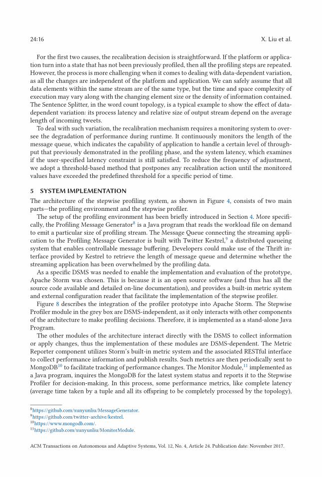
Figure 8 describes the integration of the profiler prototype into Apache Storm. The StepwiseProfiler module in the grey box are DSMS-independent, as it only interacts with other componentsof the architecture to make profiling decisions. Therefore, it is implemented as a stand-alone JavaProgram.
The other modules of the architecture interact directly with the DSMS to collect informationor apply changes, thus the implementation of these modules are DSMS-dependent. The MetricReporter component utilizes Storm’s built-in metric system and the associated RESTful interfaceto collect performance information and publish results. Such metrics are then periodically sent toMongoDB10 to facilitate tracking of performance changes. The Monitor Module,11 implemented asa Java program, inquires the MongoDB for the latest system status and reports it to the StepwiseProfiler for decision-making. In this process, some performance metrics, like complete latency(average time taken by a tuple and all its offspring to be completely processed by the topology),
8https://github.com/xunyunliu/MessageGenerator.9https://github.com/twitter-archive/kestrel.10https://www.mongodb.com/.11https://github.com/xunyunliu/MonitorModule.
ACM Transactions on Autonomous and Adaptive Systems, Vol. 12, No. 4, Article 24. Publication date: November 2017.
A Stepwise Auto-Profiling Method for Performance Optimization 24:17
Fig. 8. The integration of the profiler prototype into Apache Storm.
number of data emitted, and operator capacity can be directly used in the stepwise profiler. Somemetrics, however, require certain post-processing in the Monitor Module. For example, there is nodefault definition for throughput among the built-in metrics. Thus, to avoid ambiguity, the MonitorModule calculates the overall throughput of a streaming application based on the observed numberof acknowledgments or emitted data per unit of time, depending on whether the application adoptsreliable message processing or not.
We also utilize some useful features of Storm in the process of generating and applying newconfigurations. Specifically, Storm not only supports reading parallelism setting of operators froman external configuration file, but also provides a command line tool (Storm API) to manage thetopology with additional operational parameters. The stepwise profiler thus makes use of the Con-figuration Modifier component, which is implemented as a script file, to pack up all the profilingdecisions in a deployment configuration file, and then invokes the command line tool to submitthe application with the updated deployment scheme for the next round of profiling. The round-robin scheduler guarantees that tasks are evenly distributed across Worker Nodes and that load isequally distributed among machines.
Another aspect relating to implementation is the management of operator states during thescaling-up process. We do not address dynamic stream rerouting and live state migration, sincethe Configuration Modifier relies on the rebalance command to apply any deployment changes.This command, as a built-in Storm functionality, essentially pauses the application during theredeployment and then restarts it from scratch with the new configuration, following the so-calledPause and Resume protocol (Heinze et al. 2014a). As our current prototype treats stateful operatorsthe same way as stateless operators in terms of scaling, the management of operator states is nottransparently handled by the profiling framework. Therefore, it is required that stateful operatorspreserve their states at the application level when the rebalance command is triggered, and theseoperators should also be initialized with the previous states when the application is restarted.However, there are some advanced mechanisms proposed in the literature that enable application-agnostic state management and interruption-free operator scaling, which is discussed inSection 7.
6 PERFORMANCE EVALUATION
We have conducted three different sets of experiments to validate the effectiveness of ourprototype.
ACM Transactions on Autonomous and Adaptive Systems, Vol. 12, No. 4, Article 24. Publication date: November 2017.
24:18 X. Liu et al.
Fig. 9. Structure of the synthetic Micro-benchmark topologies.
(1) The first experiment presented in Section 6.2 evaluates whether the stepwise profilingeffectively applies to a variety of streaming applications and if it fulfills the other goalsdiscussed in Section 2.
(2) The second one in Section 6.3 assesses the scalability of our prototype and showcases itsruntime overhead under relative large test cases.
(3) The last experiment in Section 6.4 investigates the effect of different parameters on theprofiler performance, based on which we suggest default preferences.
6.1 Experiment Setup
The experiment environment is set up on a private cloud running OpenStack. The environmentconsists of three IBM X3500 M4 machines, and each machine is equipped with 2× Intel XeonE5-2620 Processor (6 [email protected]), 64GB RAM and 2.1TB HDD. The virtual cluster deployedon the physical environment is composed of a control machine, a ZooKeeper node, and severalprocessing nodes. The first two nodes are “m1.large” (4 VCPU and 8GB RAM), while the rest of theprocessing nodes are “m1.medium” (2 VCPU and 4GB RAM per machine). The control machinehost the Stepwise Profiler, Profiling Message Generator, and the Message Queue components ofthe architecture to avoid possible interference to the profiling result.
6.1.1 Test Applications. We adapt six streaming topologies as our evaluation applications.12
These include three synthetic topologies (collectively referred to as Micro-benchmark) and threereal-world streaming applications: Word Count (WC), Synthetic Word Count (SWC), and Twit-ter Sentiment Analysis (TSA). All applications are configured with acknowledgments enabled totrack the complete latency, and they process the same type of workload to calculate compara-ble throughput. The profiling stream used for performance test is recursively generated from asingle workload file, which contains 159,620 tweets in JSON format collected from 24/03/2014 to14/04/2014. In addition, these applications are carefully tuned to avoid out-of-memory crash andother failures due to insufficient resource allocation, so the only potential consequence of improperconfiguration is suboptimal performance, rather than abrupt termination of the application.
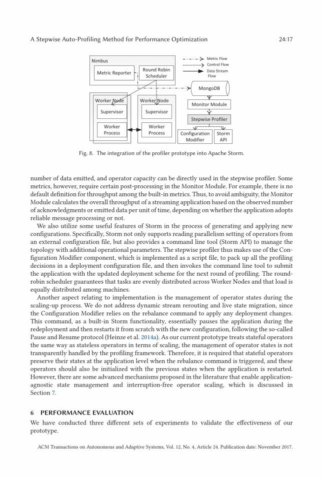
Micro-benchmark: the micro-benchmark topology is synthetically designed to evaluate how thestepwise profiler generalises to different topology structures. As shown in Figure 9, it covers threecommon structure patterns: Linear, Diamond, and Star, where an operator has (1) one-input-one-output, (2) multiple-outputs or multiple-inputs, and (3) multiple-inputs-multiple-outputs,respectively.
In addition, the execute method of each operator is implemented in three different patterns toreflect diverse time-space complexities. Some operators are (1) CPU bound, as they invoke a random
12In the following section, we use application and topology interchangeably to refer to the streaming logic developed on
Apache Storm.
ACM Transactions on Autonomous and Adaptive Systems, Vol. 12, No. 4, Article 24. Publication date: November 2017.
A Stepwise Auto-Profiling Method for Performance Optimization 24:19
Fig. 10. Structure of the Twitter Sentiment Analysis (TSA) topology.
number generation method Math.random() 10, 000 times for each tuple received. Some are (2) I/O
bound with only a JSON parse operation applied on the incoming tuple, so they spend more timeon waiting for I/O operations rather than actually processing the current data. The rest of theoperators are (3) Sojourn time-bond, which sleep for 5ms upon any tuple receipt. These operatorsare introduced to mimic the cases where an external service is requested to complete the tupletransaction. Consequently, they demand almost no CPU and memory usages on the executionplatform, but still consume a substantial sojourn time for each incoming tuple to be processed.
All these operators have a function implemented to read the operator selectivity13 from the ex-ternal configuration file. Higher selectivity can be specified to produce saturated network usages,so I/O bound operators could be overwhelmed by large internal streams.
Word Count and Synthetic Word Count: the Word Count topology is illustrated in Figure 3. TheSynthetic Word Count topology adds a Waiting operator (a bolt14 in Storm’s terminology) betweenthe Kestrel Spout and the JSON Parser, where each incoming tuple is kept for 1ms before beingsent to the next operator. Therefore, WC and SWC are actually two different implementations forthe same streaming application.
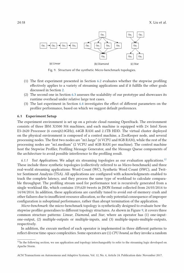
Twitter Sentiment Analysis: we adapted this topology from a mature open-source project hostedon Github15 with the structure shown in Figure 10. It has 11 bolts constituting a tree-style topologythat has 8 stages in depth. The processing logic of this application is straightforward: once a newtweet is pulled into the system through Kestrel Spout (Op1), it is first stored by a file writer (Op2)and examined by a language detector (Op3) to identify which language it uses. If it is writtenin English, then there is a sentiment analysis bolt (Op4) that splits the sentence and calculatesthe sentimental score for the whole content using AFINN,16 which contains a list of words withtheir pre-computed sentiment valence from minus five (negative) to plus five (positive). There arealso several bolts to count the average sentiment result (Op5, Op6) and to rank the most frequenthashtags occurring over a specific time window (Op7 ∼ Op11).
6.1.2 Evaluation Methodology. We use throughput and complete latency to quantitatively eval-uate the performance of streaming applications. Higher monitored throughput indicates higherperformance potential, as long as the complete latency satisfies the desired target. In other words,if a streaming application has demonstrated throughput T in the profiling environment, we canconfidently assume that it has ability to process any throughput T ′ < T without violating the la-tency constraint, unless the profiling knowledge needs to be recalibrated. Therefore, to probe themaximum sustainable throughput, the profiling environment feeds the applications with large in-puts, until the performance hits its highest stable point before recording it as the observed value.
The measurement of performance metrics first requires the test application to be deployed onthe execution platform. Apart from complying with the generated configuration, we also set thenumber of workers to one per machine and the number of tasks to be the same as the number of
13The selectivity is defined as the ratio between the number of output tuples produced and the number of tuples consumed
by this operator.14Operators in Storm are called spouts—if they are data sources—or bolts otherwise.15https://github.com/kantega/storm-twitter-workshop.16http://www2.imm.dtu.dk/pubdb/views/publication_details.php?id=6010.
ACM Transactions on Autonomous and Adaptive Systems, Vol. 12, No. 4, Article 24. Publication date: November 2017.
24:20 X. Liu et al.
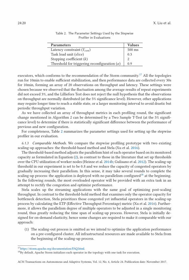
Table 2. The Parameter Settings Used by the Stepwise
Profiler in Evaluations
Parameters Values
Latency constraint (Ycon ) 500 msTask load unit (slice) 0.3Stopping coefficient (k) 2Threshold for triggering reconfiguration (α ) 0.9
executors, which conforms to the recommendation of the Storm community.17 All the topologiesrun for 10min to enable sufficient stabilization, and then performance data are collected every 30sfor 10min, forming an array of 20 observations on throughput and latency. These settings werechosen because we observed that the fluctuation among the average results of repeat experimentsdid not exceed 3%, and the Lilliefors Test does not reject the null hypothesis that the observationson throughput are normally distributed (at the 5% significance level). However, other applicationsmay require longer time to reach a stable state, or a larger monitoring interval to avoid drastic butperiodic throughput variation.
As we have collected an array of throughput metrics in each profiling round, the significantchange mentioned in Algorithm 2 can be determined by a Two Sample T-Test (at the 5% signifi-cance level) to determine if there is statistically significant difference between the performance ofprevious and new configuration.
For completeness, Table 2 summarizes the parameter settings used for setting up the stepwiseprofiler in our evaluation.
6.1.3 Comparable Methods. We compare the stepwise profiling prototype with two existingscaling-up approaches: the threshold-based method and Stela (Xu et al. 2016).
The threshold-based method adjusts the parallelism hint of each operator based on its monitoredcapacity as formulated in Equation (2), in contrast to those in the literature that set up thresholdsover the CPU utilization of worker nodes (Heinze et al. 2014b; Gulisano et al. 2012). The scaling-upthreshold in our experiment is set to be 0.8 and we reduce the capacity of congested operators bygradually increasing their parallelism. In this sense, it may take several rounds to complete thescaling-up process: the application is deployed with no parallelism configured18 at the beginning.In the following rounds, the most overloaded operator will be provided with an extra task in anattempt to rectify the congestion and optimize performance.
Stela scales up the streaming applications with the same goal of optimizing post-scalingthroughput. In contrast to the threshold-hold method that examines only the operator capacity forbottleneck detection, Stela prioritizes those congested yet influential operators in the scaling-upprocess by calculating the ETP (Effective Throughput Percentage) metric (Xu et al. 2016). Further-more, it allows the parallelism degree of multiple operators to be adjusted in a single monitoringround, thus greatly reducing the time span of scaling-up process. However, Stela is initially de-signed for on-demand elasticity, hence some changes are required to make it comparable with ourapproach:
(1) The scaling-out process is omitted as we intend to optimize the application performanceon a pre-configured cluster. All infrastructural resources are made available to Stela fromthe beginning of the scaling-up process.
17https://storm.apache.org/documentation/FAQ.html.18By default, Apache Storm initializes each operator in the topology with one task for execution.
ACM Transactions on Autonomous and Adaptive Systems, Vol. 12, No. 4, Article 24. Publication date: November 2017.
A Stepwise Auto-Profiling Method for Performance Optimization 24:21
(2) A single monitoring round of Stela corresponds to an on-demand scaling request in itsoriginal form, which may involve multiple scaling-up iterations. During each iteration,Stela calculates the ETP for all operators and assigns a new task to the operator with thehighest ETP. Before proceeding to the next iteration, the table of ETP is updated withprojected values that estimate the consequence of scaling, such as the projected input rateand the processing rate of the targeted operator.
(3) Since the estimation of ETP is prone to error propagation, we limit the maximum numberof scaling-up attempts in a monitoring round tom, which is the number of worker nodesavailable at the infrastructure level. In this way, the efficacy of the scaling algorithm isassured as the table of ETP is revised with monitored data everym iterations; and the riskof over-scaling is controlled, since each machine will be assigned with no more than onenew task in a single monitoring round.
6.2 Applicability Evaluation
In the applicability experiment, all the topologies are executed in six worker nodes. We configuredthe micro-benchmark topologies with different resource complexities to examine how applicationdiversity affects the performance optimization process. Specifically, the Linear topology incorpo-rates only CPU-bound operators so the whole application is bound by available CPU resources;while the Star topology consists of only I/O bound operators, causing its performance to be boundby communication capability.19 The Diamond topology, on the other hand, is a hybrid streamingapplication that includes all sorts of operators (1 CPU bound, 1 I/O bound, and 2 Sojourn time-bound) in the intermediate tier, making its bottleneck more difficult to identify and resolve in thescaling-up process.
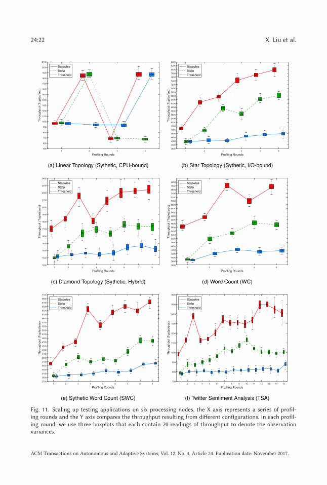
The results in Figure 11 show that the stepwise profiler successfully scales up the targetedtopologies. In particular, the Linear topology reaches its maximum throughput at 1876 with theparallelism set as (1, 2, 2, 2),20 which is 95.7% higher than its initial throughput performanceyielded by (1, 1, 1, 1). It took four rounds for the scaling-up process to converge: the stepwiseprofiler tried the configuration of (1, 3, 3, 3) at round 3, but it then rejected such configurationchange due to the observed performance degradation. Note that the operator capacity profiling isentirely omitted in this scaling-up process, as the measured operator latencies have all fallen intothe vicinity of the monitored MinLp by a factor of 2.
Being I/O intensive in nature, the Star topology requires much higher parallelism settings toenable satisfactory performance, which consequently leads to a longer scaling-up process. In ourevaluation, the scaling-up process took six rounds to finish, with the parallelism finally set as(3, 3, 48, 24, 24) delivering 64% higher throughput than the first round. Thanks to the homogeneityof operator implementation, there is no need to fine tune the operator capacities as the stoppingcondition on latency has been met.
The Diamond topology, in contrast, spent three rounds in the third step to further scale up theI/O bound operator (Op3). During the process of platform capability profiling, stepwise profilersuccessfully determines the right parallelism for CPU-bound and Sojourn time-bound operators;however, it underestimates the number of tasks for Op3 and causes it to be the throughput bottle-neck. The reason of insufficient scaling is that Equation (1) made a conservative decimal conversionby using slice of 0.3, which prevents Op3 from scaling more than four times faster than the otheroperators. We will shed more light on the effect of parameter selection in Section 6.4.
19For I/O bound topologies (e.g., Star), we set Ycon to 100 ms to reflect stricter timeliness requirement.20From left to right, each number corresponds to the number of tasks of each operator in the Linear Topology.
ACM Transactions on Autonomous and Adaptive Systems, Vol. 12, No. 4, Article 24. Publication date: November 2017.
24:22 X. Liu et al.
Fig. 11. Scaling up testing applications on six processing nodes, the X axis represents a series of profil-
ing rounds and the Y axis compares the throughput resulting from different configurations. In each profil-
ing round, we use three boxplots that each contain 20 readings of throughput to denote the observation
variances.
ACM Transactions on Autonomous and Adaptive Systems, Vol. 12, No. 4, Article 24. Publication date: November 2017.
A Stepwise Auto-Profiling Method for Performance Optimization 24:23
In addition, by interpreting the scaling-up process of real-world streaming applications, we con-clude that our method is consistently better than the other two scaling approaches in the followingthree aspects. First, stepwise profiling exploits the inherent feature of a streaming application andthus has a more reasonable starting point of profiling comparing to the other two baseline meth-ods, which by contrast determine the initial configuration only based on the topology structure.Figure 11 illustrates that the application feature profiling for WC, SWC, and TSA improves theperformance by 45%, 21.1%, and 25% at the beginning, respectively.
Second, as platform capability profiling collectively adjusts the parallelism hints for a set ofoperators, it significantly enhances the performance gains obtained from the first few profilingrounds. On average, the relative performance improvement observed from the first four roundsin our method is 2.48 times as large as that of Stela, and 11.63 times compared to that of thethreshold-based method. Besides, despite having the ability to tune multiple parallelism hints ina single round, Stela’s estimation-based algorithm could lead to incorrect scaling decision, forexample, it added new tasks to logic-dependent operators and caused performance degradation atround 10 in Figure 11(f). To make things worse, there is no reversal mechanism to rollback thewrong move.
Finally, the stopping condition introduced in Section 4.3 greatly limited the number of profilingrounds. Specifically, stepwise profiling stops trying new configuration in TSA, because there aresuccessive revocations that show increasing parallelism hint no longer benefits the performance.In WC and SWC, the profiler execution terminates when the latencies for each bolt dropped into arange of (0, 2∗MinLp], which indicates that the application has been sufficiently scaled up. In theend, our approach is 34.1%, 40.1%, 31.9% better than the best alternative in terms of the throughputresulted from the final configuration, respectively.
With the performance information profiled, the quality of different topology implementationsin terms of their performance potentials can be easily observed. In this case, SWC is consistentlyworse than WC as the former implementation only reaches 86.8% throughput of the latter and ittakes more effort (9 rounds vs. 5 rounds) to probe a reasonable configuration.
6.3 Scalability Evaluation
We explore the scalability of our stepwise profiling prototype in two dimensions. The firstdimension is topology complexity, which examines how the increasing number of operators inthe topology affects the scaling-up process. The other dimension is platform size, which checksif the prototype is able to deliver a reasonably higher post-scaling performance using moreresources. Meanwhile, we also compare stepwise profiling with Stela in terms of the minimalresources needed to reach a specific performance target.
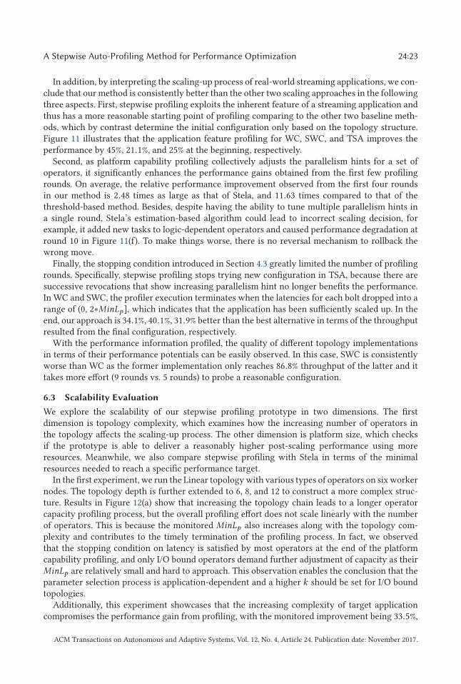
In the first experiment, we run the Linear topology with various types of operators on six workernodes. The topology depth is further extended to 6, 8, and 12 to construct a more complex struc-ture. Results in Figure 12(a) show that increasing the topology chain leads to a longer operatorcapacity profiling process, but the overall profiling effort does not scale linearly with the numberof operators. This is because the monitored MinLp also increases along with the topology com-plexity and contributes to the timely termination of the profiling process. In fact, we observedthat the stopping condition on latency is satisfied by most operators at the end of the platformcapability profiling, and only I/O bound operators demand further adjustment of capacity as theirMinLp are relatively small and hard to approach. This observation enables the conclusion that theparameter selection process is application-dependent and a higher k should be set for I/O boundtopologies.
Additionally, this experiment showcases that the increasing complexity of target applicationcompromises the performance gain from profiling, with the monitored improvement being 33.5%,
ACM Transactions on Autonomous and Adaptive Systems, Vol. 12, No. 4, Article 24. Publication date: November 2017.
24:24 X. Liu et al.
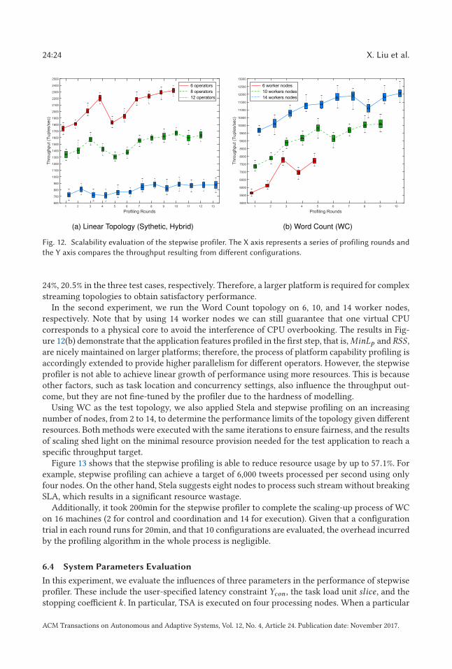
Fig. 12. Scalability evaluation of the stepwise profiler. The X axis represents a series of profiling rounds and
the Y axis compares the throughput resulting from different configurations.
24%, 20.5% in the three test cases, respectively. Therefore, a larger platform is required for complexstreaming topologies to obtain satisfactory performance.
In the second experiment, we run the Word Count topology on 6, 10, and 14 worker nodes,respectively. Note that by using 14 worker nodes we can still guarantee that one virtual CPUcorresponds to a physical core to avoid the interference of CPU overbooking. The results in Fig-ure 12(b) demonstrate that the application features profiled in the first step, that is,MinLp and RSS ,are nicely maintained on larger platforms; therefore, the process of platform capability profiling isaccordingly extended to provide higher parallelism for different operators. However, the stepwiseprofiler is not able to achieve linear growth of performance using more resources. This is becauseother factors, such as task location and concurrency settings, also influence the throughput out-come, but they are not fine-tuned by the profiler due to the hardness of modelling.
Using WC as the test topology, we also applied Stela and stepwise profiling on an increasingnumber of nodes, from 2 to 14, to determine the performance limits of the topology given differentresources. Both methods were executed with the same iterations to ensure fairness, and the resultsof scaling shed light on the minimal resource provision needed for the test application to reach aspecific throughput target.
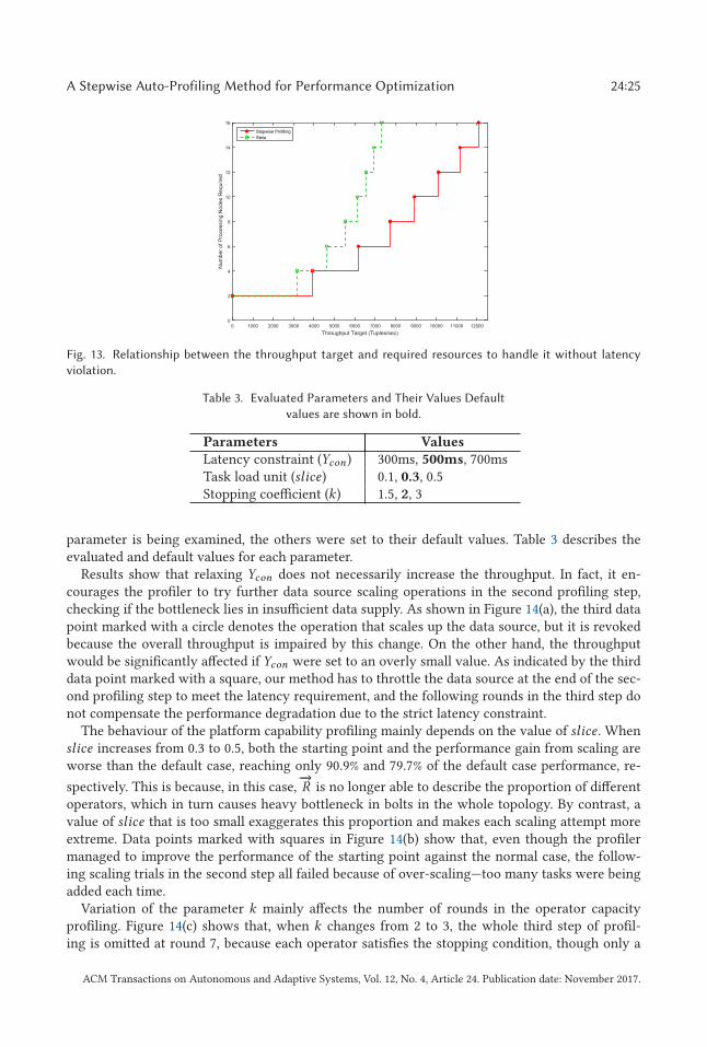
Figure 13 shows that the stepwise profiling is able to reduce resource usage by up to 57.1%. Forexample, stepwise profiling can achieve a target of 6,000 tweets processed per second using onlyfour nodes. On the other hand, Stela suggests eight nodes to process such stream without breakingSLA, which results in a significant resource wastage.
Additionally, it took 200min for the stepwise profiler to complete the scaling-up process of WCon 16 machines (2 for control and coordination and 14 for execution). Given that a configurationtrial in each round runs for 20min, and that 10 configurations are evaluated, the overhead incurredby the profiling algorithm in the whole process is negligible.
6.4 System Parameters Evaluation
In this experiment, we evaluate the influences of three parameters in the performance of stepwiseprofiler. These include the user-specified latency constraint Ycon , the task load unit slice , and thestopping coefficient k . In particular, TSA is executed on four processing nodes. When a particular
ACM Transactions on Autonomous and Adaptive Systems, Vol. 12, No. 4, Article 24. Publication date: November 2017.
A Stepwise Auto-Profiling Method for Performance Optimization 24:25
Fig. 13. Relationship between the throughput target and required resources to handle it without latency
violation.
Table 3. Evaluated Parameters and Their Values Default
values are shown in bold.
Parameters Values
Latency constraint (Ycon ) 300ms, 500ms, 700msTask load unit (slice) 0.1, 0.3, 0.5Stopping coefficient (k) 1.5, 2, 3
parameter is being examined, the others were set to their default values. Table 3 describes theevaluated and default values for each parameter.
Results show that relaxing Ycon does not necessarily increase the throughput. In fact, it en-courages the profiler to try further data source scaling operations in the second profiling step,checking if the bottleneck lies in insufficient data supply. As shown in Figure 14(a), the third datapoint marked with a circle denotes the operation that scales up the data source, but it is revokedbecause the overall throughput is impaired by this change. On the other hand, the throughputwould be significantly affected if Ycon were set to an overly small value. As indicated by the thirddata point marked with a square, our method has to throttle the data source at the end of the sec-ond profiling step to meet the latency requirement, and the following rounds in the third step donot compensate the performance degradation due to the strict latency constraint.
The behaviour of the platform capability profiling mainly depends on the value of slice . Whenslice increases from 0.3 to 0.5, both the starting point and the performance gain from scaling areworse than the default case, reaching only 90.9% and 79.7% of the default case performance, re-
spectively. This is because, in this case,−→R is no longer able to describe the proportion of different
operators, which in turn causes heavy bottleneck in bolts in the whole topology. By contrast, avalue of slice that is too small exaggerates this proportion and makes each scaling attempt moreextreme. Data points marked with squares in Figure 14(b) show that, even though the profilermanaged to improve the performance of the starting point against the normal case, the follow-ing scaling trials in the second step all failed because of over-scaling—too many tasks were beingadded each time.
Variation of the parameter k mainly affects the number of rounds in the operator capacityprofiling. Figure 14(c) shows that, when k changes from 2 to 3, the whole third step of profil-ing is omitted at round 7, because each operator satisfies the stopping condition, though only a
ACM Transactions on Autonomous and Adaptive Systems, Vol. 12, No. 4, Article 24. Publication date: November 2017.
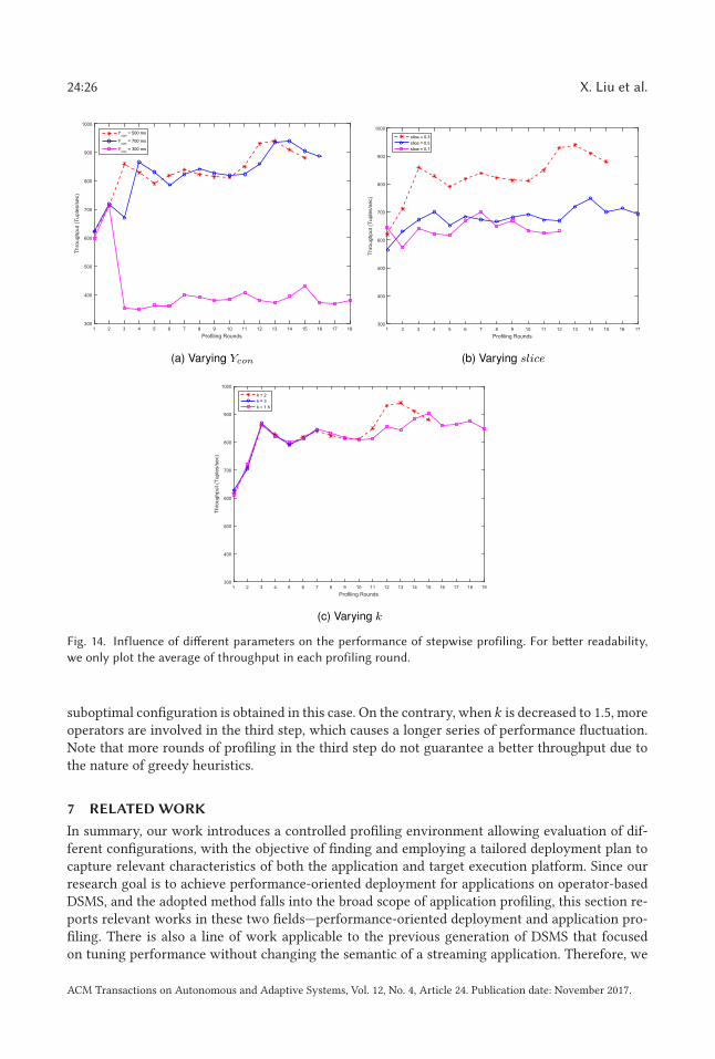
24:26 X. Liu et al.
Fig. 14. Influence of different parameters on the performance of stepwise profiling. For better readability,
we only plot the average of throughput in each profiling round.
suboptimal configuration is obtained in this case. On the contrary, when k is decreased to 1.5, moreoperators are involved in the third step, which causes a longer series of performance fluctuation.Note that more rounds of profiling in the third step do not guarantee a better throughput due tothe nature of greedy heuristics.
7 RELATED WORK
In summary, our work introduces a controlled profiling environment allowing evaluation of dif-ferent configurations, with the objective of finding and employing a tailored deployment plan tocapture relevant characteristics of both the application and target execution platform. Since ourresearch goal is to achieve performance-oriented deployment for applications on operator-basedDSMS, and the adopted method falls into the broad scope of application profiling, this section re-ports relevant works in these two fields—performance-oriented deployment and application pro-filing. There is also a line of work applicable to the previous generation of DSMS that focusedon tuning performance without changing the semantic of a streaming application. Therefore, we
ACM Transactions on Autonomous and Adaptive Systems, Vol. 12, No. 4, Article 24. Publication date: November 2017.
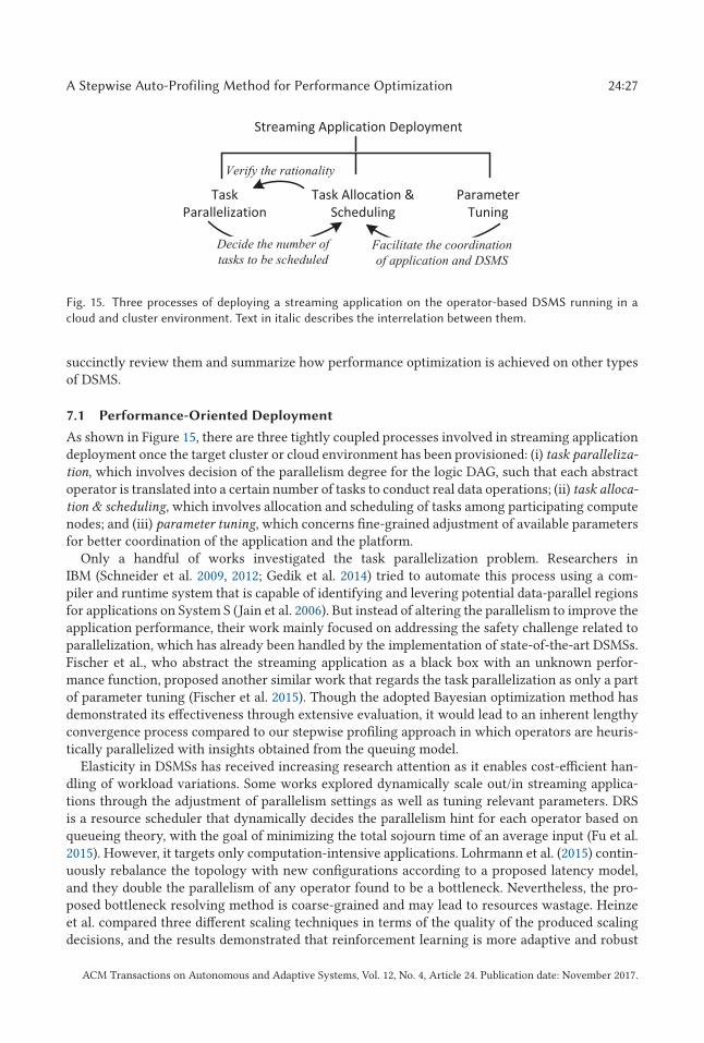
A Stepwise Auto-Profiling Method for Performance Optimization 24:27
Fig. 15. Three processes of deploying a streaming application on the operator-based DSMS running in a
cloud and cluster environment. Text in italic describes the interrelation between them.
succinctly review them and summarize how performance optimization is achieved on other typesof DSMS.
7.1 Performance-Oriented Deployment
As shown in Figure 15, there are three tightly coupled processes involved in streaming applicationdeployment once the target cluster or cloud environment has been provisioned: (i) task paralleliza-
tion, which involves decision of the parallelism degree for the logic DAG, such that each abstractoperator is translated into a certain number of tasks to conduct real data operations; (ii) task alloca-
tion & scheduling, which involves allocation and scheduling of tasks among participating computenodes; and (iii) parameter tuning, which concerns fine-grained adjustment of available parametersfor better coordination of the application and the platform.
Only a handful of works investigated the task parallelization problem. Researchers inIBM (Schneider et al. 2009, 2012; Gedik et al. 2014) tried to automate this process using a com-piler and runtime system that is capable of identifying and levering potential data-parallel regionsfor applications on System S (Jain et al. 2006). But instead of altering the parallelism to improve theapplication performance, their work mainly focused on addressing the safety challenge related toparallelization, which has already been handled by the implementation of state-of-the-art DSMSs.Fischer et al., who abstract the streaming application as a black box with an unknown perfor-mance function, proposed another similar work that regards the task parallelization as only a partof parameter tuning (Fischer et al. 2015). Though the adopted Bayesian optimization method hasdemonstrated its effectiveness through extensive evaluation, it would lead to an inherent lengthyconvergence process compared to our stepwise profiling approach in which operators are heuris-tically parallelized with insights obtained from the queuing model.
Elasticity in DSMSs has received increasing research attention as it enables cost-efficient han-dling of workload variations. Some works explored dynamically scale out/in streaming applica-tions through the adjustment of parallelism settings as well as tuning relevant parameters. DRSis a resource scheduler that dynamically decides the parallelism hint for each operator based onqueueing theory, with the goal of minimizing the total sojourn time of an average input (Fu et al.2015). However, it targets only computation-intensive applications. Lohrmann et al. (2015) contin-uously rebalance the topology with new configurations according to a proposed latency model,and they double the parallelism of any operator found to be a bottleneck. Nevertheless, the pro-posed bottleneck resolving method is coarse-grained and may lead to resources wastage. Heinzeet al. compared three different scaling techniques in terms of the quality of the produced scalingdecisions, and the results demonstrated that reinforcement learning is more adaptive and robust
ACM Transactions on Autonomous and Adaptive Systems, Vol. 12, No. 4, Article 24. Publication date: November 2017.
24:28 X. Liu et al.
than the threshold-based alternatives (Heinze et al. 2014b). Hidalgo et al. combined the threshold-based method with the Markov chain model to dynamically change the operator parallelism, sothe short-term and mid-term workload variations can be handled with reactive and predictiveapproaches, respectively (Hidalgo et al. 2017). Besides, realizing elasticity for stateful operators re-quires non-trivial efforts to handle issues such as stream rerouting and state migration. While theadopted pause-and-resume strategy is commonly seen in the literature (Castro Fernandez et al.2013; Cardellini et al. 2016; Madsen et al. 2016), there are also advanced protocols for operatormovement and state management that allow for interruption-free elasticity (Wu and Tan 2015;Matteis and Mencagli 2017; Ravindra et al. 2017). In future work, these techniques can be inte-grated in our prototype to improve its responsiveness against workload burst. As for parametertuning, Das et al. (2014) proposed a control algorithm to automatically determine the most suit-able batch for a given state, while online parameter optimization has been investigated by Heinzeet al. to deal with the situation where the application needs to be dynamically scaled as a reactionto workload changes (Heinze et al. 2015). Our target is different to all those above as we try todetermine the configuration for any streaming application given the platform that maximizes thethroughput under latency constraint.
In contrast, the task allocation and scheduling problem has received much more attention fromthe research community. Aniello et al. pioneered this area with two scheduling algorithms onApache Storm: the off-line version makes all the scheduling decisions through a static analysisof the logic DAG, while the on-line version regularly collects runtime information to sort all thecommunicating pairs of tasks, with an attempt to sequentially co-locate them in the same node toreduce communication cost (Aniello et al. 2013). Inspired by this idea, many works extended theon-line algorithm by adding some other aspects into consideration, such as scheduling overhead,resource awareness, and energy efficiency. Chatzistergiou et al. proposed a linear time task allo-cation algorithm to adaptively reconfigure task locations in the presence of environment changes,resulting in a significant improvement from the existing quadratic time solutions (Chatzistergiouand Viglas 2014). Fischer et al. presented an application agnostic algorithm that supports schedul-ing of large-scale task graphs with regard to the communication pattern, the problem of minimiz-ing inter-node messages is thus translated into a graph-partitioning problem, which can be solvedby the use of METIS algorithm (Fischer and Bernstein 2015).
On the other hand, there are also some articles that explored the area of resource aware sched-uling and put an emphasis on worker node consolidation. The algorithm used in T-Storm (Xuet al. 2014) tries to minimize both inter-node and inter-process traffic while avoiding overloadingthe dwindled worker nodes. Similarly, Peng et al. (2015) considered the task scheduling as a varia-tion of the Knapsack problem with several hard/soft resource constraints, so it can be solved by theapplication of linear programming given that the user has provided the resource demand and avail-ability information. Apart from the common target of reducing communication cost, Re-Stream,an energy-efficient resource scheduling mechanism by Sun et al., proposed the minimization ofenergy consumption as long as the response latency meets SLA requirements. This is achieved byan analytic model that depicts the relationship among energy consumption, response time, andthe resource utilization (Sun et al. 2014, 2015). Our work can be used along with these methodsabove as none of them address the issue of task parallelization.
Besides cluster and cloud environments that are the target of our approach, the problem of de-ploying streaming application on multi-core systems and distributed networks has also been dis-cussed by several works. Hormati et al. (2009) proposed a framework that dynamically adapts ap-plications to the changing characteristics of the multi-core resources to maximize the throughput,using a hybrid approach of static compilation and dynamic configurations adjustments. Similarly,Suleman et al. (2010) introduced a framework to tune the parallelism for each stage in a processing
ACM Transactions on Autonomous and Adaptive Systems, Vol. 12, No. 4, Article 24. Publication date: November 2017.
A Stepwise Auto-Profiling Method for Performance Optimization 24:29
pipeline using a hill-climbing algorithm that can both save time and reduce the number of usedcores. As for network deployment, Cardellini et al. (2015) extended Apache Storm with a self-adaptive distributed scheduling mechanism, which allows execution of streaming applications ona geographically distributed environment with a certain level of QoS guarantee.
7.2 Application Profiling
Application profiling is a technique that actively extracts and evaluates the characteristics of appli-cations, for example, the space or time complexity, to facilitate the use of computing resources. Theprofiled data sets can be either low-level usage traces of CPU, memory, and network bandwidth, orhigh level metrics that are part of application SLA, such as throughput, latency, and fault-toleranceability (Weingartner et al. 2015). To make sure that the application profile would accurately reflectresource needs, the profiling process is normally conducted in a dedicated profiling environmentfollowing the MAPE-K autonomic loop (Monitor, Analyze, Plan, Execute-Knowledge) (Kephartand Chess 2003), which enables controllable organization of input data and eliminates variationfactors that would affect the result collection and analysis.
Most of the state-of-the-art programming IDEs, such as Microsoft Visual Studio and Eclipse,provide tools to aid in determining bottlenecks in the code that affect the overall performanceof a program. However, the research community has gone way beyond code-level performanceprofiling. Urgaonkar et al. (2002) investigated the overbooking problem by the use of applicationprofiling, which helps to deliver an accurate estimate of resource needs for application compo-nents co-located on shared hosts. Do et al. (2011) achieved better virtual machine placement witha performance prediction model derived from the application profile. To obtain higher profilingaccuracy, they identify background load, which is the interference of other applications into con-sideration. Shen et al. (2015) used profiling to automate the detection of performance bottleneckfor web applications with a large set of input parameters. Similar to our work, the proposed pro-filing method is able to heuristically search the best configuration that maximizes the objectiveperformance function. Qian et al. (2011) developed a tool that profiles the cross-layer interactionwithin mobile applications, aiming to better reveal the performance and energy bottlenecks hiddenin the inefficient resource usages. Still, our work is different to them in that we adopt the profil-ing method to guide the deployment process of streaming application, while the above-mentionedmodels mostly target batch-oriented (MapReduce) or interactive-oriented (web and mobile) appli-cations and thus cannot be directly applied in streaming applications.
It is also worth mentioning that we have carefully designed the stepwise profiler to avoid DSMSlock-in. Besides Apache Storm, there are many operator-based DSMSs that support general pur-pose stream processing, including Microsoft TimeStream (Qian et al. 2013), Apache Samza, ApacheFlink (Lohrmann et al. 2014), and Twitter Heron (Kulkarni et al. 2015). None of them has a built-infeature to automatically decide the parallel configuration for a particular application, and thus allof them can benefit from the proposed profiler.
7.3 Other Performance Optimization Techniques
It has been more than a decade since the first generation DSMSs, including Aurora (Abadi et al.2003), Niagara (Chen et al. 2000), and Telegraph (Chandrasekaran et al. 2003), were introduced tofacilitate the development and deployment of streaming applications. Along with the increasingadoption of DSMS, various optimization techniques have been developed to improve the perfor-mance of applications without changing their topology or semantics.
Operator placement optimization, for example, is a process of assigning operators to specifichosts and cores to reach a trade-off between communication cost and resource contention. Thoughit is still a kind of adjustment in application layout rather than spreading and scheduling tasks (as
ACM Transactions on Autonomous and Adaptive Systems, Vol. 12, No. 4, Article 24. Publication date: November 2017.
24:30 X. Liu et al.
discussed in Section 7.1), operator placement in previous generation DSMS regards each operatoras an indivisible entity that can only appear in one place at a time. In this context, Gordon et al.designed a software-programmable substrate capable of generating custom communication code toreduce message hops when placing operator on multi-core systems (Gordon et al. 2002). Auerbachet al. proposed a placement mechanism to guarantee that operators compiled for an FPGA willalways be placed on hosts with FPGAs (Auerbach et al. 2010). In addition to resource matching,Wolf et al. (2008) considered other constraints during the placement process, such as licensing andsecurity requirement.
Load balancing is another commonly used optimization technique to evenly distribute work-load across available resources. This requires either a balanced operator placement plan or aruntime mechanism to dynamically assign stream tuples to operators. As examples of these twoapproaches, Xing et al. migrated conflicting operators that experience load spikes at the sametime to separate locations to avoid resource contention and thus improving load balance (Xinget al. 2005), while Amini et al. (2006) discussed the use of back-pressure in System S to compensateskews found in runtime.
However, these optimization techniques are no longer applicable to state-of-the-art streamingapplications built on top of operator-based DSMS, as the implementation of DSMS has greatlyevolved towards scalability and robustness, causing operator placement and load balancing to relyheavily on the parallelization and scheduling of tasks that constitute the operator.
8 CONCLUSIONS AND FUTURE WORK
We proposed a streaming application profiler that consists of three steps, namely (i) applicationfeature profiling, which aims to identify the complexity and task load for each operator; (ii) plat-form capability profiling, which endeavours to scale up the application with the knowledge learnedfrom the previous step; and (iii) operator capacity profiling, which makes necessary amendmentson fine-grained level to further improve performance of the application. Our profiler can be usedto scale up streaming application, build the relationship between the underlying resources andthe performance metrics, and further evaluate the choice of resource provision. An evaluation ofa profiler prototype applied to three real-world applications showed that our approach is able toautomatically improve the throughput up to 40.1% compared to Stela, a state-of-the-art alternativescaling approach.
As for future work, we plan to devise auto-scaling policies on top of the profiling results, whichenables dynamic adjustment of provisioned resources according to real-time performance require-ments of a variety of workloads. Since responsiveness is a critical criterion for realizing runtime-adaptation, the envisioned auto-scaling policies should be built on top of interruption-free scalingmechanisms such as dynamic stream rerouting and live state migration. Deploying the streamingapplications on the cloud and exploiting the use of VM with different configurations are also on ourfuture plan. A distinct advantage of using cloud resources is that it supports resource customiza-tion. Therefore, there is a great potential in performance optimization to place different operatorson tailored cloud instances that fit their special needs, such as hosting computation-intensive op-erators on fast CPU nodes and placing operators with intensive intercommunication in the samevirtual node to minimize communication overhead. We would also like to leverage different cloudpricing models (On-Demand, Reserved, Spot) with the aim of minimizing the monetary cost ofstream processing, making cloud a preferable platform for deployment of streaming applications.
REFERENCES
Daniel J. Abadi, Don Carney, Ugur Çetintemel, Mitch Cherniack, Christian Convey, Sangdon Lee, Michael Stonebraker,
Nesime Tatbul, and Stan Zdonik. 2003. Aurora: A new model and architecture for data stream management. VLDB
J. 12, 2 (Aug. 2003), 120–139.
ACM Transactions on Autonomous and Adaptive Systems, Vol. 12, No. 4, Article 24. Publication date: November 2017.
A Stepwise Auto-Profiling Method for Performance Optimization 24:31
Lisa Amini, Navendu Jain, Anshul Sehgal, Jeremy Silber, and Olivier Verscheure. 2006. Adaptive control of extreme-scale
stream processing systems. In Proceedings of the 26th IEEE International Conference on Distributed Computing Systems
(ICDCS’06). IEEE Computer Society, 71–77.
Leonardo Aniello, Roberto Baldoni, and Leonardo Querzoni. 2013. Adaptive online scheduling in storm. In Proceedings of
the 7th ACM International Conference on Distributed Event-Based Systems (DEBS’13). ACM, 207–218.
Joshua Auerbach, David F. Bacon, Perry Cheng, and Rodric Rabbah. 2010. Lime: A java-compatible and synthesizable
language for heterogeneous architectures. In Proceedings of the ACM International Conference on Object-Oriented Pro-
gramming Systems Languages and Applications (OOPSLA’10). ACM, 89–108.
Paolo Bellavista, Antonio Corradi, Andrea Reale, and Nicola Ticca. 2014. Priority-based resource scheduling in distributed
stream processing systems for big data applications. In Proceedings of the 2014 IEEE/ACM 7th International Conference
on Utility and Cloud Computing (UCC’14). IEEE, 363–370.
Michael Cammert, Christoph Heinz, Jurgen Kramer, Bernhard Seeger, Sonny Vaupel, and Udo Wolske. 2007. Flexible multi-
threaded scheduling for continuous queries over data streams. In Proceedings of the 23rd IEEE International Conference
on Data Engineering Workshop (ICDE’07). IEEE, 624–633.
Valeria Cardellini, Vincenzo Grassi, Francesco Lo Presti, and Matteo Nardelli. 2015. Distributed QoS-aware scheduling
in storm. In Proceedings of the 9th ACM International Conference on Distributed Event-Based Systems (DEBS’15). ACM,
344–347.
Valeria Cardellini, Matteo Nardelli, and Dario Luzi. 2016. Elastic stateful stream processing in storm. In Proceedings of the
2016 International Conference on High Performance Computing Simulation (HPCS’16). IEEE, 583–590.
Raul Castro Fernandez, Matteo Migliavacca, Evangelia Kalyvianaki, and Peter Pietzuch. 2013. Integrating scale out and fault
tolerance in stream processing using operator state management. In Proceedings of the 2013 ACM SIGMOD International
Conference on Management of Data (SIGMOD’13). ACM, 725–736.
Sirish Chandrasekaran, Owen Cooper, Amol Deshpande, Michael J. Franklin, Joseph M. Hellerstein, Wei Hong, Sailesh
Krishnamurthy, Samuel R. Madden, Fred Reiss, and Mehul A. Shah. 2003. TelegraphCQ: Continuous dataflow process-
ing. In Proceedings of the 2003 ACM SIGMOD International Conference on Management of Data (SIGMOD’03). ACM,
668–668.
Andreas Chatzistergiou and Stratis D. Viglas. 2014. Fast heuristics for near-optimal task allocation in data stream processing
over clusters. In Proceedings of the 23rd ACM International Conference on Conference on Information and Knowledge
Management (CIKM’14). ACM, 1579–1588.
Jianjun Chen, David J. DeWitt, Feng Tian, and Yuan Wang. 2000. NiagaraCQ: A scalable continuous query system for inter-
net databases. In Proceedings of the 2000 ACM SIGMOD International Conference on Management of Data (SIGMOD’00).
ACM, 379–390.
Tathagata Das, Yuan Zhong, Ion Stoica, and Scott Shenker. 2014. Adaptive stream processing using dynamic batch sizing.
In Proceedings of the ACM Symposium on Cloud Computing (SOCC’14). ACM, 1–13.
Anh Vu Do, Junliang Chen, Chen Wang, Young Choon Lee, A. Y. Zomaya, and Bing Bing Zhou. 2011. Profiling applica-
tions for virtual machine placement in clouds. In Proceedings of the IEEE International Conference on Cloud Computing
(CLOUD’11). IEEE, 660–667.
Lorenz Fischer and Abraham Bernstein. 2015. Workload scheduling in distributed stream processors using graph partition-
ing. In Proceedings of the 2015 IEEE International Conference on Big Data (BigData’15). IEEE Computer Society, 124–133.
Lorenz Fischer, Shen Gao, and Abraham Bernstein. 2015. Machines tuning machines: Configuring distributed stream pro-
cessors with Bayesian Optimization. In Proceedings of the 2015 IEEE International Conference on Cluster Computing
(CLUSTER’15). IEEE, 22–31.
Tom Z. J. Fu, Jianbing Ding, Richard T. B. Ma, Marianne Winslett, Yin Yang, and Zhenjie Zhang. 2015. DRS: Dynamic
resource scheduling for real-time analytics over fast streams. In Proceedings of the IEEE 35th International Conference on
Distributed Computing Systems (ICDCS’15). IEEE, 411–420.
Bugra Gedik, Scott Schneider, Martin Hirzel, and Kun-Lung Wu. 2014. Elastic scaling for data stream processing. IEEE
Trans. Parallel Distrib. Syst. 25, 6 (June 2014), 1447–1463.
Michael I. Gordon, William Thies, Michal Karczmarek, Jasper Lin, Ali S. Meli, Andrew A. Lamb, Chris Leger, Jeremy Wong,
Henry Hoffmann, David Maze, and Saman Amarasinghe. 2002. A stream compiler for communication-exposed archi-
tectures. In Proceedings of the 10th International Conference on Architectural Support for Programming Languages and
Operating Systems (ASPLOS’02). ACM, 291–303.
Vincenzo Gulisano, Ricardo Jimenez-Peris, Marta Patino-Martinez, Claudio Soriente, and Patrick Valduriez. 2012. Stream-
Cloud: An elastic and scalable data streaming system. IEEE Transactions on Parallel and Distributed Systems 23, 12 (Dec.
2012), 2351–2365.
Thomas Heinze, Leonardo Aniello, Leonardo Querzoni, and Zbigniew Jerzak. 2014a. Cloud-based data stream process-
ing. In Proceedings of the 8th ACM International Conference on Distributed Event-Based Systems (DEBS’14). ACM, 238–
245.
ACM Transactions on Autonomous and Adaptive Systems, Vol. 12, No. 4, Article 24. Publication date: November 2017.
24:32 X. Liu et al.
Thomas Heinze, Valerio Pappalardo, Zbigniew Jerzak, and Christof Fetzer. 2014b. Auto-scaling techniques for elastic data
stream processing. In Proceedings of the 8th ACM International Conference on Distributed Event-Based Systems (DEBS’14).
ACM, 318–321.
Thomas Heinze, Lars Roediger, Andreas Meister, Yuanzhen Ji, Zbigniew Jerzak, and Christof Fetzer. 2015. Online parameter
optimization for elastic data stream processing. In Proceedings of the 6th ACM Symposium on Cloud Computing (SoCC’15).
ACM, 276–287.
Nicolas Hidalgo, Daniel Wladdimiro, and Erika Rosas. 2017. Self-adaptive processing graph with operator fission for elastic
stream processing. Journal of Systems and Software 127 (2017), 205–216.
Amir H. Hormati, Yoonseo Choi, Manjunath Kudlur, Rodric Rabbah, Trevor Mudge, and Scott Mahlke. 2009. Flextream:
Adaptive compilation of streaming applications for heterogeneous architectures. In Proceedings of the 18th International
Conference on Parallel Architectures and Compilation Techniques (PACT’09). ACM, 214–223.
Waldemar Hummer, Benjamin Satzger, and Schahram Dustdar. 2013. Elastic stream processing in the cloud. Wiley Interdisc.
Rev.: Data Min. Knowl. Discov. 3, 5 (Sept. 2013), 333–345.
Navendu Jain, Lisa Amini, Henrique Andrade, Richard King, Yoonho Park, Philippe Selo, and Chitra Venkatramani. 2006.
Design, implementation, and evaluation of the linear road benchmark on the stream processing core. In Proceedings of
the ACM SIGMOD International Conference on Management of Data (SIGMOD’06). ACM, 431–442.
Jeffrey O. Kephart and David M. Chess. 2003. The vision of autonomic computing. Computer 36, 1 (Jan. 2003), 41–50.
Sanjeev Kulkarni, Nikunj Bhagat, Maosong Fu, Vikas Kedigehalli, Christopher Kellogg, Sailesh Mittal, Jignesh M. Patel,
Karthik Ramasamy, and Siddarth Taneja. 2015. Twitter heron: Stream processing at scale. In Proceedings of the ACM
SIGMOD International Conference on Management of Data (SIGMOD’15). ACM, 239–250.
Teng Li, Jian Tang, and Jielong Xu. 2015. A predictive scheduling framework for fast and distributed stream data processing.
In Proceedings of the 2015 IEEE International Conference on Big Data (BigData’15). IEEE Computer Society, 333–338.
Bjn Lohrmann, Peter Janacik, and Odej Kao. 2015. Elastic stream processing with latency guarantees. In Proceedings of the
2015 IEEE 35th International Conference on Distributed Computing Systems (ICDCS’15). IEEE, 399–410.
Bjrn Lohrmann, Daniel Warneke, and Odej Kao. 2014. Nephele streaming: Stream processing under QoS constraints at
scale. Cluster Comput. 17, 1 (2014), 61–78.
Kasper Grud Skat Madsen, Yongluan Zhou, and Li Su. 2016. Enorm: Efficient window-based computation in large-scale
distributed stream processing systems. In Proceedings of the 10th ACM International Conference on Distributed and Event-
based Systems (DEBS’16). ACM, 37–48.
Tiziano De Matteis and Gabriele Mencagli. 2017. Proactive elasticity and energy awareness in data stream processing.
Journal of Systems and Software 127 (2017), 302–319.
Lory Al Moakar, Alexandros Labrinidis, and Panos K. Chrysanthis. 2012. Adaptive class-based scheduling of continuous
queries. In Proceeding of the 28th IEEE International Conference on Data Engineering Workshop (ICDE’12). IEEE, 289–294.
Boyang Peng, Mohammad Hosseini, Zhihao Hong, Reza Farivar, and Roy Campbell. 2015. R-Storm: Resource-aware sched-
uling in Storm. In Proceedings of the 16th Annual Middleware Conference (Middleware’15). ACM, 149–161.
Feng Qian, Zhaoguang Wang, Alexandre Gerber, Zhuoqing Mao, Subhabrata Sen, and Oliver Spatscheck. 2011. Profiling
resource usage for mobile applications: A cross-layer approach. In Proceedings of the 9th International Conference on
Mobile Systems, Applications, and Services (MobiSys’11). ACM, 321–334.
Zhengping Qian, Yong He, Chunzhi Su, Zhuojie Wu, Hongyu Zhu, Taizhi Zhang, Lidong Zhou, Yuan Yu, and Zheng Zhang.
2013. TimeStream: Reliable stream computation in the cloud. In Proceedings of the European Conference on Computer
Systems (EuroSys’13). ACM, 1–14.
Sajith Ravindra, Miyuru Dayarathna, and Sanath Jayasena. 2017. Latency aware elastic switching-based stream processing
over compressed data streams. In Proceedings of the 8th ACM/SPEC on International Conference on Performance Engi-
neering (ICPE’17). ACM, 91–102.
Scott Schneider, Henrique Andrade, Bugra Gedik, Alain Biem, and Kun-Lung Wu. 2009. Elastic scaling of data parallel
operators in stream processing. In Proceedings of the IEEE International Symposium on Parallel Distributed Processing
(IPDPS’09). IEEE, 1–12.
Scott Schneider, Martin Hirzel, Bugra Gedik, and Kun-Lung Wu. 2012. Auto-parallelizing stateful distributed streaming
applications. In Proceedings of the 21st International Conference on Parallel Architectures and Compilation Techniques
(PACT’12). ACM, 53–64.
Du Shen, Qi Luo, Denys Poshyvanyk, and Mark Grechanik. 2015. Automating performance bottleneck detection using
search-based application profiling. In Proceedings of the 2015 International Symposium on Software Testing and Analysis
(ISSTA’15). ACM, 270–281.
Muhammad Aater Suleman, Moinuddin K. Qureshi, Khubaib, and Yale N. Patt. 2010. Feedback-directed pipeline parallelism.
In Proceedings of the 19th International Conference on Parallel Architectures and Compilation Techniques (PACT’10). ACM,
147–156.
ACM Transactions on Autonomous and Adaptive Systems, Vol. 12, No. 4, Article 24. Publication date: November 2017.

A Stepwise Auto-Profiling Method for Performance Optimization 24:33
Dawei Sun, Ge Fu, Xinran Liu, and Hong Zhang. 2014. Optimizing data stream graph for big data stream computing in
cloud datacenter environments. Int. J. Adv. Comput. Technol. 6, 5 (2014), 53–65.
Dawei Sun, Guangyan Zhang, Songlin Yang, Weimin Zheng, Samee U. Khan, and Keqin Li. 2015. Re-Stream: Real-time and
energy-efficient resource scheduling in big data stream computing environments. Info. Sci. 319 (Oct. 2015), 92–112.
Bhuvan Urgaonkar, Prashant Shenoy, and Timothy Roscoe. 2002. Resource overbooking and application profiling in shared
hosting platforms. SIGOPS Oper. Syst. Rev. 36, SI (Dec. 2002), 239–254.
Rafael Weingartner, Gabriel Beims Brascher, and Carlos Becker Westphall. 2015. Cloud resource management: A survey
on forecasting and profiling models. J. Netw. Comput. Appl. 47 (2015), 99–106.
Joel Wolf, Nikhil Bansal, Kirsten Hildrum, Sujay Parekh, Deepak Rajan, Rohit Wagle, Kun-Lung Wu, and Lisa Fleischer.
2008. SODA: An optimizing scheduler for large-scale stream-based distributed computer systems. In Proceedings of the
9th ACM/IFIP/USENIX International Conference on Middleware (Middleware’08). Springer-Verlag, 306–325.
Yingjun Wu and Kian-Lee Tan. 2015. ChronoStream: Elastic stateful stream computation in the cloud. In Proceedings of the
2015 IEEE 31st International Conference on Data Engineering. IEEE, 723–734.
Ying Xing, Stan Zdonik, and Jeong-Hyon Hwang. 2005. Dynamic load distribution in the borealis stream processor. In
Proceedings of the 21st International Conference on Data Engineering (ICDE’05). IEEE Computer Society, 791–802.
Jielong Xu, Zhenhua Chen, Jian Tang, and Sen Su. 2014. T-Storm: Traffic-aware online scheduling in storm. In Proceedings
of the 2014 IEEE 34th International Conference on Distributed Computing Systems (ICDCS’14). IEEE Computer Society,
535–544.
Le Xu, Boyang Peng, and Indranil Gupta. 2016. Stela: Enabling stream processing systems to scale-in and scale-out on-
demand. In Proceedings of the 2016 IEEE International Conference on Cloud Engineering (IC2E’16). IEEE, 22–31.
Received November 2016; revised May 2017; accepted July 2017
ACM Transactions on Autonomous and Adaptive Systems, Vol. 12, No. 4, Article 24. Publication date: November 2017.