A Statistical Approach to Map Matching Using Road Network

A statistical approach to map matching using road network geometry,topology and vehicular motion constraints

Oliver Pink, Britta Hummel

Institut fur Mess- und Regelungstechnik

Universitat Karlsruhe (TH), 76128 Karlsruhe, Germany

{pink,hummel}@mrt.uka.de

Abstract— This paper presents a method for reliable match-ing of position and orientation measurements from a standardGPS receiver to a digital map. By incorporating road networktopology in the matching process using a hidden Markov model,an optimum position and orientation history can be computedfrom a sequence of GPS measurements.

Increased robustness is achieved by introducing constraintsfor vehicular motion in an extended Kalman filter and byreconstructing the original road network from the digital mapusing cubic spline interpolation. The proposed method deliversrobust matching results for standard inner-city scenarios andgives a reliable estimate of the optimal position history evenfor severely disturbed GPS measurements.

I. INTRODUCTION

Recent years have shown a tremendous increase in demand

of mobile geographic information systems. Starting from

built-in and hand-held navigation systems, a large number

of applications in intelligent transportation systems like fleet

management, road traffic management or electronic toll col-

lection has evolved.

An essential task for these applications is the assign-

ment of a vehicle position measurement to a position in

a digital map, the so-called map matching. Many of these

applications, do not only require a reliable estimate of the

current vehicle position, but also an estimate of the driven

path. Considering the correct charging of road tolls, posterior

knowledge of the driven path is essential, while a false

intermediate position estimate is tolerable.

Previous work on map matching has focused especially on

fast and reliable estimation of the current vehicle position in a

digital map. An overview on earlier work can be found in [1].

More recent work on map matching has focused especially

on robustness and reconstruction of the vehicle path [9], [2].

In our previous work, we have already presented a method

for robust, GPS only map matching [6] that has already

shown promising results in determining the vehicle position

history. In this paper, we will present an improved method

that allows for robust estimation of the vehicle position

history over long periods of time and even with severely

disturbed GPS measurements.

The remainder of this paper will be organized as follows.

In section II, the objective of this paper is formulated and

our system setup will be introduced. In section III, filtering

of the raw GPS measurements in an extended Kalman filter

is described. Reconstruction of the road geometry from the

digital map is explained in section IV and the representation

of road topology in a hidden Markov model is presented in

section V. The map matching process itself is explained in

section VI and experimental results are given in section VII.

Section VIII gives a summary and concludes the paper.

II. PRELIMINARIES

Our approach will be described in two steps: First a

generic map matching problem will be formulated, and sec-

ond a suitable statistical representation of the measurement

uncertainties will be derived.

The generic problem can be described as finding the

optimal vehicle path on a road network for a given set of

vehicle position and orientation measurements with known

uncertainties of both the map and the position and orientation

estimates. This part will be described as a standard Bayesian

classification task that is independent of the particular sensor

platform chosen. Sensor characteristics are incorporated in

a representation of measurement uncertainties. The sensor

setup we will use only consists of a standard GPS receiver

and an industry-standard digital map. We chose this setup

because it is the smallest possible set of sensors that is used

in practice, e.g. for portable navigation devices. The main

idea is that using additional sensors or sensors with a higher

precision will very likely yield better map matching results.

The GPS receiver delivers one measurement for vehicle

position and orientation per second. While there is no un-

certainty of the vehicle orientation available, the horizontal

dilution of precision (HDOP) can be used as a coarse esti-

mate for the position uncertainties. However, the orientation

uncertainty can be modeled as inversely proportional to

vehicle speed.

The digital representation of the road network is compliant

to the GDF standard [7]. Road network topology is described

by nodes and edges, where every edge represents one road

segment and a node represents connections between those

road elements. Additional properties may restrict certain

driving maneuvers for both nodes and edges, such as one-

way road elements or right-turn only at intersections.

Road network geometry is represented by the geographic

positions of the nodes and by additional shape points that

may be assigned to an edge. Shape points are usually placed

to keep the lateral deviation under a certain threshold, but

the exact placement is vendor-specific. However, both nodes

and shape points are assumed to lie exactly on the center

line of the road.

Proceedings of the 11th International IEEEConference on Intelligent Transportation SystemsBeijing, China, October 12-15, 2008

1-4244-2112-1/08/$20.00 ©2008 IEEE 862

Authorized licensed use limited to: Universitatsbibliothek Karlsruhe. Downloaded on July 2, 2009 at 03:49 from IEEE Xplore. Restrictions apply.

First published in:

EVA-STAR (Elektronisches Volltextarchiv – Scientific Articles Repository) http://digbib.ubka.uni-karlsruhe.de/volltexte/1000011968

III. VEHICLE STATE ESTIMATION

The vehicle state x that will be needed for the map match-

ing algorithm consists of a 2-dimensional position estimate

[x, y]T , a heading angle estimate ϕ and the corresponding

uncertainties, i.e. the 3 × 3 covariance matrix Σx.

Instead of directly using the measurements from the GPS

receiver as state estimates, we will use a simple constant

velocity and constant yaw rate model in an extended Kalman

filter for state estimation. The continuous-time system model

is determined according to figure 1:⎡⎢⎢⎢⎢⎣

xyϕvη

⎤⎥⎥⎥⎥⎦ =

⎡⎢⎢⎢⎢⎣

−v · sin(ϕ)v · cos(ϕ)

η00

⎤⎥⎥⎥⎥⎦ , (1)

where x and y are the vehicle position, ϕ is the vehicle

heading and v is the vehicle speed. The yaw rate is denoted

η to avoid confusion with the state variable ϕ.

The corresponding discrete-time approximation with sam-

pling time T is⎡⎢⎢⎢⎢⎣

xk+1

yk+1

ϕk+1

vk+1

ηk+1

⎤⎥⎥⎥⎥⎦ =

⎡⎢⎢⎢⎢⎣

xk − vk · T · sin(ϕk)yk + vk · T · cos(ϕk)

ϕk + ηk · Tvk

ηk

⎤⎥⎥⎥⎥⎦ . (2)

A detailed description of the extended Kalman filter can

be found in literature, e.g. in [10].

The first three elements of the Kalman Filter state vector

are the desired vehicle state x for the map matching process.

The corresponding upper left 3×3 sub-matrix of the Kalman

filter state covariance matrix is the desired covariance matrix

for map matching Σx.

The use of a vehicle model with very low dynamics

is mainly justified by the lack of highly dynamic sensor

data in our system. However, the system model may be

easily extended to account for different sensor characteristics

and application specific needs, e.g. dead reckoning using

odometry for built-in systems.

ϕ (0)v

x(0)

v

ϕ t

y

x

x(t)

.

.

ϕ (t)

Fig. 1. Vehicular motion for constant velocity and yaw rate.

IV. ROAD NETWORK GEOMETRY

Reconstruction of the road network from a given set of

shape points is commonly done by linear interpolation of the

shape points. Subsequent matching of the vehicle position

to the interpolated road network typically yields position

residuals in the range of a few meters. Heading residuals,

however, can easily reach 45◦ during intersection traversal.This may lead to ambiguities or even false matchings in

some situations. Figure 2(a) shows an example of such an

ambiguous situation, where three positions in the map have

the same distance and orientation difference to the assumed

vehicle position. The ambiguity can easily be resolved by

using higher-order interpolation as shown in figure 2(b).

?

(a) Single position estimate.

?

?

?

(b) Sequence of position estimates.

Fig. 2. Example of an ambiguous map matching situation. The red arrowdenotes the vehicle position and heading estimate, the green arrows denotepossible map matching results. Left image: linear interpolation, right image:cubic interpolation.

As figure 2(b) shows, the occurrence of such ambiguities

has a direct impact on matching robustness. In case of linear

interpolation, the given sequence of GPS positions results

in two vehicle paths with the same probability. Higher-order

interpolation would lead to a single matching result.Unfortunately, current digital maps do not give any in-

formation about road curvature. Instead, we will exploit the

knowledge that, according to e.g. the german road construc-

tion guidelines [4]), roads are typically built with smooth

curvature change. Furthermore, we know that our road will

run exactly through its starting node p0, the n given shape

points pk, k = 1..n and its ending node pn+1.

863


Instead of linearly interpolating adjacent shape points,

we will therefore use a cubic spline polynomial for every

pair of adjacent shape points. Furthermore, we will require

smooth curvature at all transitions between interpolation

polynomials.

A nice way to assure that the interpolating polynomials run

exactly through the given shape points is to use the Hermite

formulation of the spline polynomial, where two of the four

control points are just the desired starting and ending points

(see e.g. [11] for a detailed explanation). For a given set of

n shape points si, i = 1, ..., n, we get n − 1 interpolation

polynomials

pi(λ) =(2λ3 − 3λ2 + 1

) · si(0)+

(−2λ3 + 3λ2) · si(1)

+(λ3 − 2λ2 + λ

) · s′i(0)+

(λ3 − λ2

) · s′i(1) ,

(3)

where λ ∈ [0, 1].Requiring C2 continuity delivers a system of 2n − 2

equations for the unknown 2n tangent vectors s′i(0) and

s′i(1), i = 1, ..., n. Together with the natural spline condition

s′′0(0) = 0 and s′′(n−1)(1) = 0, we get a tridiagonal system of

linear equations that can be solved for the unknown tangents.

An implementation of this solution can be found e.g. in [8].

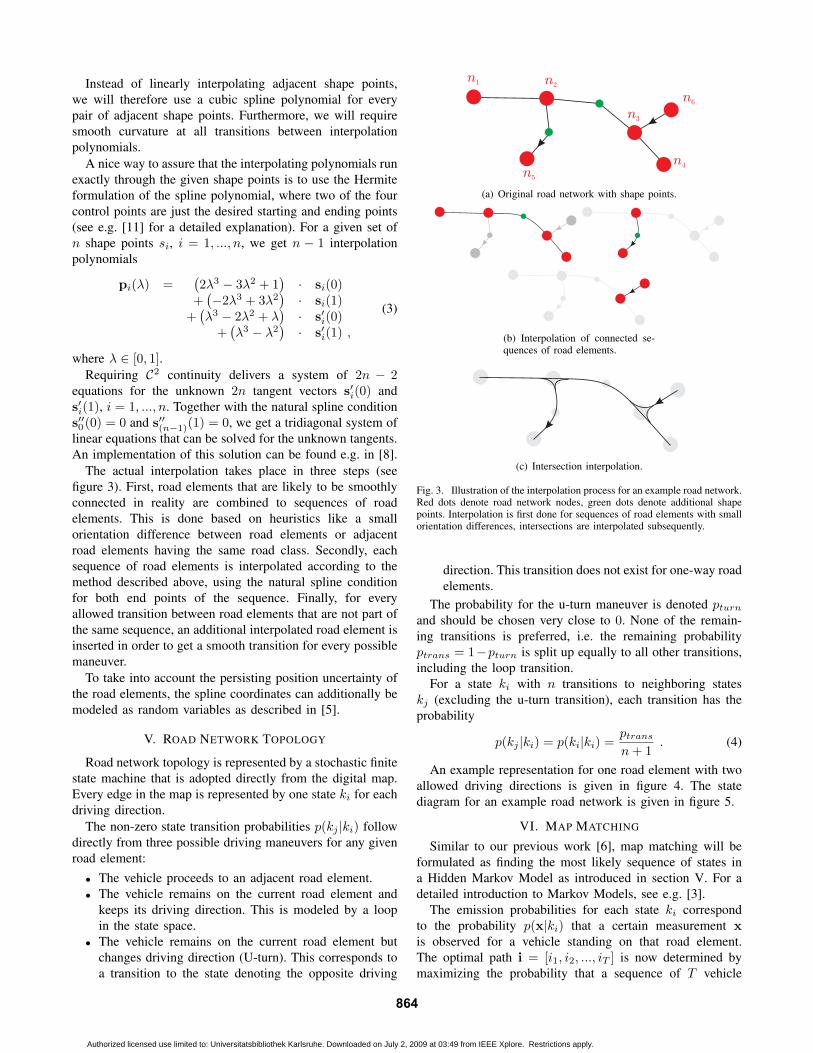
The actual interpolation takes place in three steps (see

figure 3). First, road elements that are likely to be smoothly

connected in reality are combined to sequences of road

elements. This is done based on heuristics like a small

orientation difference between road elements or adjacent

road elements having the same road class. Secondly, each

sequence of road elements is interpolated according to the

method described above, using the natural spline condition

for both end points of the sequence. Finally, for every

allowed transition between road elements that are not part of

the same sequence, an additional interpolated road element is

inserted in order to get a smooth transition for every possible

maneuver.

To take into account the persisting position uncertainty of

the road elements, the spline coordinates can additionally be

modeled as random variables as described in [5].

V. ROAD NETWORK TOPOLOGY

Road network topology is represented by a stochastic finite

state machine that is adopted directly from the digital map.

Every edge in the map is represented by one state ki for each

driving direction.

The non-zero state transition probabilities p(kj |ki) follow

directly from three possible driving maneuvers for any given

road element:

• The vehicle proceeds to an adjacent road element.

• The vehicle remains on the current road element and

keeps its driving direction. This is modeled by a loop

in the state space.

• The vehicle remains on the current road element but

changes driving direction (U-turn). This corresponds to

a transition to the state denoting the opposite driving

n1 n

2

n3

n4

n5

n6

(a) Original road network with shape points.

(b) Interpolation of connected se-quences of road elements.

(c) Intersection interpolation.

Fig. 3. Illustration of the interpolation process for an example road network.Red dots denote road network nodes, green dots denote additional shapepoints. Interpolation is first done for sequences of road elements with smallorientation differences, intersections are interpolated subsequently.

direction. This transition does not exist for one-way road

elements.

The probability for the u-turn maneuver is denoted pturn

and should be chosen very close to 0. None of the remain-

ing transitions is preferred, i.e. the remaining probability

ptrans = 1−pturn is split up equally to all other transitions,

including the loop transition.

For a state ki with n transitions to neighboring states

kj (excluding the u-turn transition), each transition has the

probability

p(kj |ki) = p(ki|ki) =ptrans

n + 1. (4)

An example representation for one road element with two

allowed driving directions is given in figure 4. The state

diagram for an example road network is given in figure 5.

VI. MAP MATCHING

Similar to our previous work [6], map matching will be

formulated as finding the most likely sequence of states in

a Hidden Markov Model as introduced in section V. For a

detailed introduction to Markov Models, see e.g. [3].

The emission probabilities for each state ki correspond

to the probability p(x|ki) that a certain measurement xis observed for a vehicle standing on that road element.

The optimal path i = [i1, i2, ..., iT ] is now determined by

maximizing the probability that a sequence of T vehicle

864


5

10

00 5 10

' = {22,5º

x m[ ]

ym[

]

5

10

00 5 10

' = 0º

x m[ ]

ym[

]

5

10

00 5 10

' = 22,5º

x m[ ]

ym[

]

5

10

00 5 10

' = 45º

x m[ ]

ym[

]

5

10

00 5 10

' = 67,5º

x m[ ]

ym[

]

5

10

00 5 10

' = 90º

x m[ ]

ym[

]

5

10

00 5 10

' = 112,5º

x m[ ]

ym[

]

(a) Linear interpolation

5

10

00 5 10

' = {22,5º

x m[ ]

ym[

]

5

10

00 5 10

' = 0º

x m[ ]

ym[

]

5

10

00 5 10

' = 22,5º

x m[ ]

ym[

]

5

10

00 5 10

' = 45º

x m[ ]

ym[

]

5

10

00 5 10

' = 67,5º

x m[ ]

ym[

]

5

10

00 5 10

' = 90º

x m[ ]

ym[

]

5

10

00 5 10

' = 112,5º

x m[ ]

ym[

]

(b) Cubic interpolation

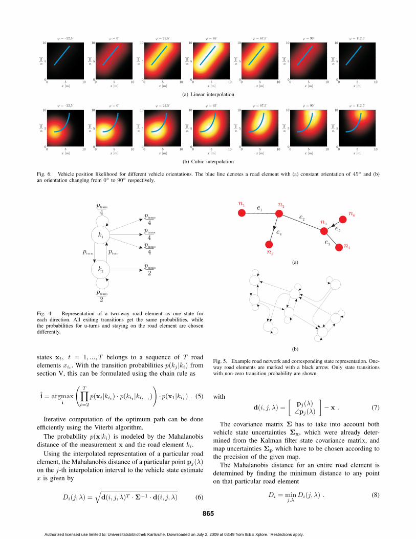
Fig. 6. Vehicle position likelihood for different vehicle orientations. The blue line denotes a road element with (a) constant orientation of 45◦ and (b)an orientation changing from 0◦ to 90◦ respectively.

k1

k2

pturn

pturn

ptrans

4

ptrans

4

ptrans

4

ptrans

2

ptrans

2

ptrans

4

Fig. 4. Representation of a two-way road element as one state foreach direction. All exiting transitions get the same probabilities, whilethe probabilities for u-turns and staying on the road element are chosendifferently.

states xt, t = 1, ..., T belongs to a sequence of T road

elements xit. With the transition probabilities p(kj |ki) from

section V, this can be formulated using the chain rule as

i = argmaxi

(T∏

t=2

p(xt|kit) · p(kit |kit−1)

)· p(x1|ki1) . (5)

Iterative computation of the optimum path can be done

efficiently using the Viterbi algorithm.

The probability p(x|ki) is modeled by the Mahalanobis

distance of the measurement x and the road element ki.

Using the interpolated representation of a particular road

element, the Mahalanobis distance of a particular point pj(λ)on the j-th interpolation interval to the vehicle state estimate

x is given by

Di(j, λ) =√

d(i, j, λ)T · Σ−1 · d(i, j, λ) (6)

e1

e2

e4

e5

e3

n1 n

2

n3

n4

n5

n6

(a)

(b)

Fig. 5. Example road network and corresponding state representation. One-way road elements are marked with a black arrow. Only state transitionswith non-zero transition probability are shown.

with

d(i, j, λ) =[

pj(λ)∠pj(λ)

]− x . (7)

The covariance matrix Σ has to take into account both

vehicle state uncertainties Σx, which were already deter-

mined from the Kalman filter state covariance matrix, and

map uncertainties Σp which have to be chosen according to

the precision of the given map.

The Mahalanobis distance for an entire road element is

determined by finding the minimum distance to any point

on that particular road element

Di = minj,λ

Di(j, λ) . (8)

865


(a) (b)

(c) (d)

Fig. 7. Map matching results for typical inner-city scenes. The sequence of GPS positions is shown in red, the current map matched position is shownin green. The blue road elements denote the optimum path.

Figure 6 illustrates the resulting position measurement

likelihood in comparison to the likelihood for linearly inter-

polated road elements as used in [6]. While the likelihoods

for linear interpolation have no distinct maxima and decrease

rapidly for increasing orientation difference, cubic interpola-

tion delivers distinct maxima over a wide range of vehicle

orientations.

VII. EXPERIMENTAL RESULTS

The proposed map matching was tested in the inner city

of Karlsruhe, Germany.

During the test run, several assignments of the vehicle

position to the wrong road element due to GPS deviations

or map errors occurred. However, the model compensated

these single outliers and returned a correct estimation of the

vehicle path history for the entire test run of more than one

hour duration.

Figure 7 shows some example results from the test run.

The GPS positions are shown in red, the optimum path

estimate is shown in blue. The map matched position for

the current time instant is shown in green.

The lateral offset in figure 7(a) is possibly caused by an

offset GPS measurement. Figures 7(b) to 7(d) show errors

due to imprecise map digitization. Errors like these are very

typical for inner-city situations and led to position offsets of

up to 40m for a short period of time. In all cases, the map

matching returns the correct path.

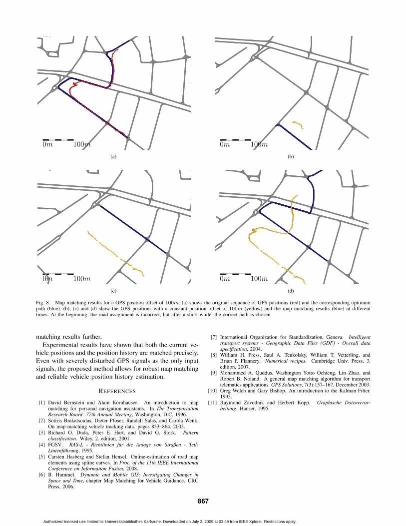
In order to evaluate the robustness of the map matching

algorithm, the original GPS sequence was manually shifted

by 100m to a random direction. The original GPS positions

are shown in figure 8(a). The map matching results are

shown in figure 8(b) to 8(d) together with the corresponding

shifted GPS measurements. At the beginning (figure 8(b)),

the positions are matched to a wrong road with the same

heading, but as soon as more GPS measurements have

supported the correct vehicle path, the correct path is chosen

(figure 8(c)). As figure 8(d) shows, the entire matched vehicle

path matches the original GPS positions very well.

VIII. CONCLUSION

We presented a robust map matching method that uses

a standard GPS receiver and an industry-standard digital

map as only input data. Increased robustness compared to

other methods was achieved by exploiting vehicular motion

constraints in an extended Kalman filter and by interpolating

the given road network using cubic splines. Representation

of the road network topology in a hidden Markov model

allows for reliable estimation of the vehicle position history

and increases robustness further.

The proposed system was designed and tested with the

smallest possible set of sensors in order to make it usable

for a wide range of applications. The map matching allows

for easy integration of further sensor information or using

higher precision map data which is likely to improve map

866


(a) (b)

(c) (d)

Fig. 8. Map matching results for a GPS position offset of 100m. (a) shows the original sequence of GPS positions (red) and the corresponding optimumpath (blue). (b), (c) and (d) show the GPS positions with a constant position offset of 100m (yellow) and the map matching results (blue) at differenttimes. At the beginning, the road assignment is incorrect, but after a short while, the correct path is chosen.

matching results further.

Experimental results have shown that both the current ve-

hicle positions and the position history are matched precisely.

Even with severely disturbed GPS signals as the only input

signals, the proposed method allows for robust map matching

and reliable vehicle position history estimation.

REFERENCES

[1] David Bernstein and Alain Kornhauser. An introduction to mapmatching for personal navigation assistants. In The TransportationResearch Board 77th Annual Meeting, Washington, D.C, 1996.

[2] Sotiris Brakatsoulas, Dieter Pfoser, Randall Salas, and Carola Wenk.On map-matching vehicle tracking data. pages 853–864, 2005.

[3] Richard O. Duda, Peter E. Hart, and David G. Stork. Patternclassification. Wiley, 2. edition, 2001.

[4] FGSV. RAS-L - Richtlinien fur die Anlage von Straßen - Teil:Linienfuhrung, 1995.

[5] Carsten Hasberg and Stefan Hensel. Online-estimation of road mapelements using spline curves. In Proc. of the 11th IEEE InternationalConference on Information Fusion, 2008.

[6] B. Hummel. Dynamic and Mobile GIS: Investigating Changes inSpace and Time, chapter Map Matching for Vehicle Guidance. CRCPress, 2006.

[7] International Organization for Standardization, Geneva. Intelligenttransport systems - Geographic Data Files (GDF) - Overall dataspecification, 2004.

[8] William H. Press, Saul A. Teukolsky, William T. Vetterling, andBrian P. Flannery. Numerical recipes. Cambridge Univ. Press, 3.edition, 2007.

[9] Mohammed A. Quddus, Washington Yotto Ochieng, Lin Zhao, andRobert B. Noland. A general map matching algorithm for transporttelematics applications. GPS Solutions, 7(3):157–167, December 2003.

[10] Greg Welch and Gary Bishop. An introduction to the Kalman Filter.1995.

[11] Raymond Zavodnik and Herbert Kopp. Graphische Datenverar-beitung. Hanser, 1995.

867


Documents

A Statistical Approach to Map Matching Using Road Network