A Statistical Approach to Gas Distribution Modelling with MobileRobots – The Kernel DM+V Algorithm

Achim J. Lilienthal, Matteo Reggente, Marco Trincavelli, Jose Luis Blanco and Javier Gonzalez

Abstract— Gas distribution modelling constitutes an idealapplication area for mobile robots, which – as intelligent mobilegas sensors – offer several advantages compared to stationarysensor networks. In this paper we propose the Kernel DM+Valgorithm to learn a statistical 2-d gas distribution model froma sequence of localized gas sensor measurements. The algorithmdoes not make strong assumptions about the sensing locationsand can thus be applied on a mobile robot that is not primarilyused for gas distribution monitoring, and also in the caseof stationary measurements. Kernel DM+V treats distributionmodelling as a density estimation problem. In contrast to mostprevious approaches, it models the variance in addition to thedistribution mean. Estimating the predictive variance entailsa significant improvement for gas distribution modelling sinceit allows to evaluate the model quality in terms of the datalikelihood. This offers a solution to the problem of groundtruth evaluation, which has always been a critical issue for gasdistribution modelling. Estimating the predictive variance alsoprovides the means to learn meta parameters and to suggestnew measurement locations based on the current model. Wederive the Kernel DM+V algorithm and present a methodfor learning the hyper-parameters. Based on real world datacollected with a mobile robot we demonstrate the consistencyof the obtained maps and present a quantitative comparison,in terms of the data likelihood of unseen samples, with analternative approach that estimates the predictive variance.

I. INTRODUCTION

Gas distribution modelling constitutes an ideal applicationarea for mobile robotics. Acting as intelligent mobile gas sen-sors, gas-sensitive robots offer several advantages comparedto stationary sensor networks. For stationary sensor networksit is a problem that the optimal sensor locations can vary withthe environmental conditions. Mobile sensors can providea distribution model with adaptive (and higher) resolution.Mobile robots that carry the sensors offer the requiredaccurate localization and computational resources to createthe distribution model on-line. Thus also the possibility todecide based on the current model which locations to observenext. Compared to human operators, mobile robots have theadvantage to carry out the required repetetive measurementprocedure without suffering from fatigue.

Gas distribution modelling with mobile robots at smallerscales has important applications in industry, science, andevery-day life. Mobile robots equipped with gas sensors aredeployed, for example, for pollution monitoring in public

Achim J. Lilienthal, Matteo Reggente and Marco Trincavelli arewith the AASS Research Centre, Dept. of Technology, OrebroUniversity, S-70182 Orebro, Sweden, achim@lilienthals.de,matteo.reggente@oru.se, mti@aass.oru.se

Jose Luis Blanco and Javier Gonzalez are with the Dept. of SystemEngineering and Automation, University of Malaga, 29071 Malaga, Spain,{jlblanco|jgonzalez}@ctima.uma.es

0 1000 2000 3000 4000 50000

0.2

0.4

0.6

0.8

1

time (s)

norm

aliz

ed s

enso

r re

spon

se

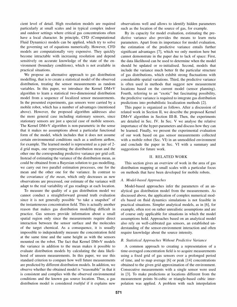
Fig. 1. Normalised raw response readings from an example trial. Corre-sponding gas distribution models are shown in Fig. 5.

areas [1], or can be used for surveillance of industrial facili-ties producing harmful gases and inspection of contaminatedareas within rescue missions.

Gas distribution modelling is the task of deriving a truthfulrepresentation of the observed gas distribution from a set ofspatially and temporally distributed measurements of relevantvariables, foremost gas concentration, but also wind andtemperature, for example. In this paper we consider the casewhere only gas sensor measurements are available.

Building gas distribution models is a very challengingtask. One main reason is that in many realistic scenarios gasis dispersed by turbulent advection. Turbulent flow createspackets of gas that follow chaotic trajectories [15]. Thisresults in a concentration field that consists of fluctuating,intermittent patches of high concentration. Fig. 1 illustratesgas concentration measurements recorded with a mobilerobot along a corridor containing a single gas source. It isimportant to note that the “noise” is dominated by the largefluctuations of the instantaneous gas distribution and not byelectronic noise of the gas sensors.

While an exact description of turbulent flow remainsan intractable problem, it is possible to describe turbulentgas distribution on average under certain assumptions [5].We therefore aim at a modelling approach that representsthe time-averaged distribution and the expected fluctuationswithout making strong assumptions about the environmentalconditions. With respect to stationary and particularly mo-bile sensing applications we further want to avoid explicitassumptions about the sensing locations so that the algorithmcan be applied on a mobile robot that is not primarily usedfor gas distribution monitoring, for example.

Many gas distribution models were developed for at-mospheric dispersion [12]. RIMPUFF, for example, is aGaussian puff model used to calculate the dispersion ofairborne materials at the mesoscale under the condition ofa moderate topography [17]. Such models cannot captureall the relevant aspects of gas propagation with a suffi-

The 2009 IEEE/RSJ International Conference onIntelligent Robots and SystemsOctober 11-15, 2009 St. Louis, USA

978-1-4244-3804-4/09/$25.00 ©2009 IEEE 570

cient level of detail. High resolution models are requiredparticularly at small scales and in typical complex indoorand outdoor settings where critical gas concentrations oftenhave a local character. In principle, CFD (ComputationalFluid Dynamics) models can be applied, which try to solvethe governing set of equations numerically. However, CFDmodels are computationally very expensive. They quicklybecome intractable with increasing resolution and dependsensitively on accurate knowledge of the state of the en-vironment (boundary conditions), which is not available inpractical situations.

We propose an alternative approach to gas distributionmodelling, that is to create a statistical model of the observeddistribution, treating the sensor measurements as randomvariables. In this paper, we introduce the Kernel DM+Valgorithm to learn a statistical two-dimensional distributionmodel from a sequence of localized sensor measurements.In the presented experiments, gas sensors were carried by amobile robot, which has a number of advantages (mentionedabove). However, the proposed algorithm addresses alsothe more general case including stationary sensors, sincestationary sensors are just a special case of mobile sensors.The Kernel DM+V algorithm is non-parametric in the sensethat it makes no assumptions about a particular functionalform of the model, which includes that it does not assumecertain environmental conditions such as a uniform airflow,for example. The learned model is represented as a pair of 2-d grid maps, one representing the distribution mean and theother one the corresponding predictive variance per grid cell.Instead of estimating the variance of the distribution mean, ascould be obtained from a Bayesian solution to gas modelling,we carry out two parallel estimation processes, one for themean and the other one for the variance. In contrast tothe covariance of the mean, which only decreases as newobservations are processed, our estimate of the variance willadapt to the real variability of gas readings at each location.

To measure the quality of a gas distribution model wecannot conduct a straightforward ground truth evaluationsince it is not generally possible “to take a snapshot” ofthe instanteneous concentration field. This is actually anotherreason that makes gas distribution modelling difficult inpractice. Gas sensors provide information about a smallspatial region only since the measurements require directinteraction between the sensor surface and the moleculesof the target chemical. As a consequence, it is usuallyimpossible to independently measure the concentration fieldat the same time and the same height as with the sensorsmounted on the robot. The fact that Kernel DM+V modelsthe variance in addition to the mean makes it possible toevaluate distribution models by calculating the data likeli-hood of unseen measurements. In this paper, we use thisstandard criterion to compare how well future measurementsare predicted by different distribution models. In addition, weobserve whether the obtained model is “reasonable” in that itis consistent and complies with the observed environmentalconditions and the known gas source location. Thus, a gasdistribution model is considered truthful if it explains new

observations well and allows to identify hidden parameterssuch as the location of the source of gas, for example.

By its capacity for model evaluation, estimating the pre-dictive variance also provides the means to learn metaparameters. Apart from its importance for model evaluation,the estimation of the predictive variance entails furthersignificant advantages [7], which we only mention here butcannot demonstrate in the paper due to lack of space: First,the data likelihood can be used to determine when the modelshould be updated or re-initialised. Second, models thatinclude the variance much better fit the particular structureof gas distributions, which exhibit strong fluctuations withconsiderable spatial variations. Third, the predictive varianceis often used in methods that suggest new measurementlocations based on the current model (sensor planning).Fourth, referring to an “exotic” but fascinating possibility,the predictive variance is required to integrate gas distributionpredictions into probabilistic localization methods [2].

This paper is organized as follows. After a discussion ofrelated work in Section II, we describe the proposed KernelDM+V algorithm in Section III-B. Then, the experimentsare detailed in Sec. IV. In Sec. V we analyse the relativeimportance of the hyper-parameters and discuss how they canbe learned. Finally, we present the experimental evaluationof our work based on gas sensor measurements collectedwith a mobile robot (Sec. VI) in an unmodified environmentand conclude the paper in Sec. VI with a summary andsuggestions for future work.

II. RELATED WORK

This section gives an overview of work in the area of gasdistribution mapping at small scales with a particular focuson methods that have been developed for mobile robots.

A. Model-based Approaches

Model-based approaches infer the parameters of an an-alytical gas distribution model from the measurements. Asdiscussed above, the application of complex numerical mod-els based on fluid dynamics simulations is not feasible inpractical situations. Simpler analytical models, as in [6], forexample, often rest on rather unrealistic assumptions and areof course only applicable for situations in which the modelassumptions hold. Approaches based on an analytical modelalso rely on well-calibrated gas sensors, an established un-derstanding of the sensor-environment interaction and oftenrequire knowledge about the source intensity.

B. Statistical Approaches Without Predictive Variance

A common approach to creating a representation of atime-averaged concentration field is to acquire measurementsusing a fixed grid of gas sensors over a prolonged periodof time, and to map average [6] or peak [14] concentrationsobtained to the given grid approximation of the environment.Consecutive measurements with a single sensor were usedin [3]. To make predictions at locations different from themeasurement points bi-cubic or triangle-based cubic inter-polation was applied. A problem with such interpolation

571

methods is that there is no means of “averaging out” in-stantaneous response fluctuations. Response values that weremeasured very close to each other appear independently inthe gas distribution map and thus the representation tendsto get more and more jagged while new measurements areadded. This can be seen in the top right of Fig. 5, wherean example of a gas distribution map resulting from usingtrilinear interpolation is shown. This map has to be comparedto the maps in the middle row in the same figure, which showequivalent distribution mean maps obtained with the KernelDM+V algorithm.

Histogram methods reflect the spatial correlation of con-centration measurements to some degree by the quantizationinto histogram bins. The 2-d histogram proposed in [4]accumulates the number of “odor hits” received in an areaassigned to the histogram bins. Odor hits are counted when-ever the response of a gas sensor exceeds a defined threshold.Disadvantages of this method include the dependency on binsize and selected threshold, that a perfectly even coverage ofthe inspected area is required, and that only binary measure-ments are used and so useful information is discarded.

Kernel extrapolation distribution mapping (“Kernel DM”)can be seen as an extension of histogram methods. Theconcentration field is represented in the form of a gridmap. Spatial integration is carried out by convolving sensorreadings and modelling the information content of the pointmeasurements with a Gaussian kernel [8].

C. Statistical Approaches With Predictive Variance

All the methods discussed so far model the average or thepeak gas concentration but not the concentration fluctuations.The Kernel DM+V algorithm proposed in this paper alsomodels the observed distribution variance per grid cell.

Another method that predicts the mean concentration andthe corresponding variance uses Gaussian process mixture(GPM) models [16]. It treats gas distribution modelling as aregression problem. Two components of the GPM representthe rather smooth “background signal” and areas of highconcentration. The components of the mixture model anda gating function, that decides to which component a datapoint belongs, are learned using Expectation Maximization(EM). In contrast to the Kernel DM+V approach, the modelis represented directly using the training data. Because itrequires the inversion of matrices that grow with the numberof training samples n, the computational complexity of learn-ing the GPM is O(n3). This is addressed in [16] by adaptivesub-sampling of the observations to obtain a sparse trainingset. The sparsification of the training data is integrated intothe EM-based learning procedure. Similarly to the KernelDM+V approach, the dependancy between nearby locationsis modelled in the GPM approach by a radially symmetric,squared exponential covariance function.

III. KERNEL DM+V

In this section, we introduce the basic ideas of the KernelDM+V algorithm and develop the underlying equations in astep-by-step manner.

A. Preliminary Remarks and Assumptions

The general gas distribution modelling problem addressedhere is to learn a predictive model of a measurement z atthe query location x

p(z|x,x1:n, z1:n), (1)

given a set of measurements z1:n taken at locations x1:n. Allthe approaches reported in Sec. II and also the Kernel DM+Vmethod proposed in this paper, are used to learn a two dimen-sional spatial model that represents time-constant structuresin the gas distribution. While the statistical approaches arenot generally restricted to represent a 2-d distribution, theassumption that the model is learned from measurements,which are generated by a time-constant random process, willnot generally be valid. However, this assumption is oftenmade in indoor environments [18] and suggestions how tohandle this issue are given in Section VIII. The sample indexi ∈ [1, n] in Eq. (1) corresponds to a time ti when themeasurement was performed. Due to the assumption thatthe samples are generated by an underlying time-constantrandom process the measurement time does not have tobe considered explicitly. The sample index i is only usedto identify individual samples. Please note that in orderto avoid calibration issues, which occur because the metaloxide gas sensors used in our experiments rarely reach theequilibrium state when exposed to the quickly fluctuatinggas distribution, we model the sensor response r directly. Inorder to compensate for drift issues and individual variationsbetween different gas sensors, “raw” response values Ri arenormalised to r ∈ [0, 1] as

ri =Ri − min({Ri})

max({Ri}) − min({Ri}) . (2)

A further assumption we make is that the response is causedby a single target gas, i.e. we do not consider problemsrelated to interferents or simultaneous mapping of multipleodours. In principle the proposed method can be extendedto the case of multiple odour sources as described in [11].In this paper, we also assume perfect knowledge about theposition xi of a sensor at the time of the measurement. Toaccount for the uncertainty about the sensor position, themethod in [10] can be used.

B. The Kernel DM+V Algorithm

Inspired by the Parzen window method [13], KernelDM+V treats distribution modelling as a density estimationproblem. As a non-parametric estimation approach, it makesno assumptions about the particular functional form of themodelled gas distribution. Gas sensor measurements areinterpreted as noisy samples from the distribution we wishto estimate given the set of samples z1:n = r1:n. In contrastto the estimation of probability density functions we do notsample from the gas distribution directly when creating thegas distribution map. It is therefore necessary to make theassumption that the trajectory of the sensors roughly coversthe available space. A perfectly even coverage, however, isnot necessary.

572

Kernel DM+V uses a uni-variate Gaussian weightingfunction N to represent the importance of measurement ri

obtained at location xi to model the gas distribution at gridcell k. First, two temporary grid maps are computed: Ω(k)

by integrating importance weights and R(k) by integratingweighted readings as

Ω(k) =∑n

i=1 N (|xi − x(k)|, σ),

R(k) =∑n

i=1 N (|xi − x(k)|, σ) · ri.(3)

Here, x(k) denotes the center of cell k and the kernel width σis a parameter of the algorithm. The integrated weights Ω(k)

are used for normalisation of the weighted readings R(k),thus even coverage is not necessary. The integrated weightsΩ(k) also provide a confidence measure for the estimate atcell k. A high value means that the estimate is based ona large number of readings recorded close to the center ofthe respective grid cell. A low value, on the other hand,means that few readings nearby the cell center are availableand that therefore a prediction has to be made using sensorreadings taken at a rather large distance. We formalize thisby introducing a confidence map α(k) computed as

α(k) = 1 − e−(Ω(k))2/σ2Ω . (4)

Confidence values α(k) are normalized to the interval [0, 1).The confidence map α(k) depends on the trajectory of thesensors, the size of grid cells c, the width of the kernel σand the scaling parameter σΩ. This map is used to computethe mean concentration estimate r(k) as

r(k) = α(k) R(k)

Ω(k)+ {1 − α(k)}r0 (5)

where r0 represents an estimate of the mean concentrationfor cells for which we do not have sufficient informationfrom nearby readings, indicated by a low value of α(k). Weset r0 to be the average over all sensor readings.

As it was mentioned above, we want to estimate the realvariability of gas readings at each location instead of thecovariance of the mean and therefore carry out a parallelestimation process. Similarly to the distribution mean map,Eq. (5), the variance map v(k) is computed from variancecontributions integrated in a further temporary map V (k)

V (k) =∑n

i=1 N (|xi − x(k)|, σ)(ri − r(k(i)))2,

v(k) = α(k) V (k)

Ω(k) + {1 − α(k)}v0

(6)

where k(i) is the cell closest to the measurement point xi,and thus r(k(i)) is the mean prediction of the model for cellk. The estimate v0 of the distribution variance in regions farfrom measurement points is computed as the average overall variance contributions.

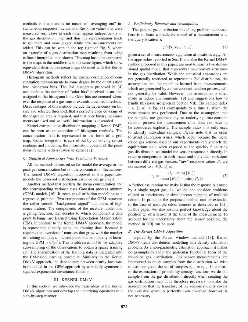
Fig. 2 shows an example of a weight map Ω(k) (top row)and the corresponding confidence map α(k) (bottom row).For narrow kernels, and large values of σΩ (left column)one can see the trajectory of the gas sensor carried by therobot, indicating that the predictions from extrapolation willonly be considered trustworthy close to actual measurement

Fig. 2. Weight map Ω(k) (top row) and the corresponding confidencemap α(k) (bottom row) obtained using the parameters σ = 0.10 m, σΩ =5.0 · N (0, 0.10) ≈ 20.0 (left column) and σ = 0.50 m, σΩ = 1.0 ·N (0, 0.50) ≈ 0.8 (right column) on a grid with cell size c = 0.05 m.

locations. For wider kernels or smaller values of σΩ (rightcolumn) the area for which predictions based on extrapola-tion are made is larger.

The complexity of computing the maps in Eq. (3) isgenerally O[n · (D

c )2] where n is the number of trainingsamples, D is the dimension of the environment and c is thecell size. In practice, we do not have to evaluate the Gaussianweighting function N for all cells and limit the region forwhich the weights are computed to a circle of radius 4σaround the measurement location. Therefore the effectivecomputational complexity is O[n · (σ

c )2]. The complexity ofcomputing the maps α(k), r(k), and v(k) in Eqs. 4, 5, and 6 isO[(D

c )2] and computing V (k) in 6 requires one pass throughthe data (O[n]), thus the overall complexity is O[n · (σ

c )2].

IV. EXPERIMENTS

We carried out gas distribution mapping experiments inwhich a robot followed a predefined sweeping trajectorycovering the area of interest. Measurements were recorded ata frequency of 1 Hz. Along its path, the robot was stopped ata pre-defined set of grid points to carry out measurements onthe spot for 10 s (outdoors) and 30 s (indoors). In this way wecan investigate how the proposed algorithm deals with thecase of a moving sensor (by using only the measurementstaken between the stops) or a situation similar to that ofa stationary sensor network (using only the measurementsfrom the stopped robot). The spacing between the grid pointswas set to values between 0.5 m to 2.0 m depending on theavailable space. The sweeping motion was performed twicein opposite directions and the robot was driven at a maximumspeed of 5 cm/s in between the stops. The gas source was asmall cup filled with ethanol.

Apart from a SICK laser range scanner used for posecorrection, the robot was equipped with an electronic noseand an anemometer (not used to compute gas distributionmaps). The electronic nose comprises six Figaro gas sensors(2×TGS 2600, TGS 2602, TGS 2611, TGS 2620, TGS 4161)

573

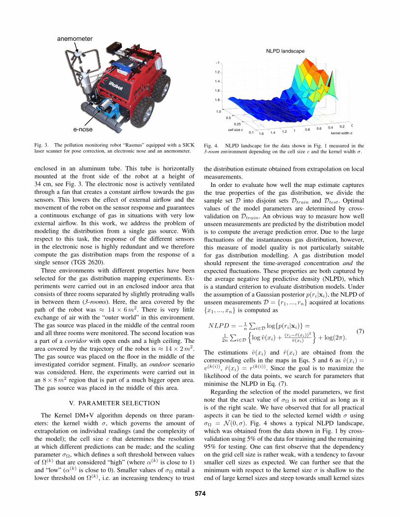
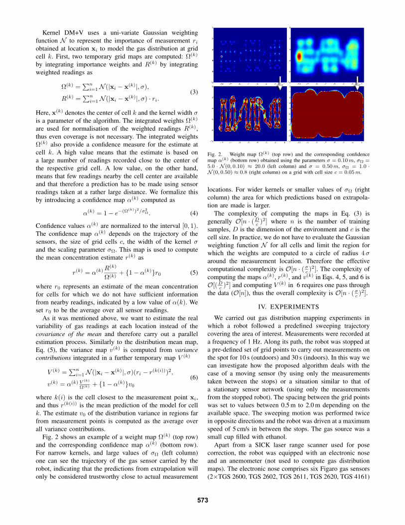
Fig. 3. The pollution monitoring robot “Rasmus” equipped with a SICKlaser scanner for pose correction, an electronic nose and an anemometer.

enclosed in an aluminum tube. This tube is horizontallymounted at the front side of the robot at a height of34 cm, see Fig. 3. The electronic nose is actively ventilatedthrough a fan that creates a constant airflow towards the gassensors. This lowers the effect of external airflow and themovement of the robot on the sensor response and guaranteesa continuous exchange of gas in situations with very lowexternal airflow. In this work, we address the problem ofmodeling the distribution from a single gas source. Withrespect to this task, the response of the different sensorsin the electronic nose is highly redundant and we thereforecompute the gas distribution maps from the response of asingle sensor (TGS 2620).

Three environments with different properties have beenselected for the gas distribution mapping experiments. Ex-periments were carried out in an enclosed indoor area thatconsists of three rooms separated by slightly protruding wallsin between them (3-rooms). Here, the area covered by thepath of the robot was ≈ 14 × 6m2. There is very littleexchange of air with the “outer world” in this environment.The gas source was placed in the middle of the central roomand all three rooms were monitored. The second location wasa part of a corridor with open ends and a high ceiling. Thearea covered by the trajectory of the robot is ≈ 14 × 2m2.The gas source was placed on the floor in the middle of theinvestigated corridor segment. Finally, an outdoor scenariowas considered. Here, the experiments were carried out inan 8× 8m2 region that is part of a much bigger open area.The gas source was placed in the middle of this area.

V. PARAMETER SELECTION

The Kernel DM+V algorithm depends on three param-eters: the kernel width σ, which governs the amount ofextrapolation on individual readings (and the complexity ofthe model); the cell size c that determines the resolutionat which different predictions can be made; and the scalingparameter σΩ, which defines a soft threshold between valuesof Ω(k) that are considered “high” (where α(k) is close to 1)and “low” (α(k) is close to 0). Smaller values of σΩ entail alower threshold on Ω(k), i.e. an increasing tendency to trust

0.1

0.25

0.5

1.0

00.20.40.60.811.21.41.6

1.8

1.6

1.4

1.2

−1

kernel width σ

NLPD landscape

cell size c

Fig. 4. NLPD landscape for the data shown in Fig. 1 measured in the3-room environment depending on the cell size c and the kernel width σ.

the distribution estimate obtained from extrapolation on localmeasurements.

In order to evaluate how well the map estimate capturesthe true properties of the gas distribution, we divide thesample set D into disjoint sets Dtrain and Dtest. Optimalvalues of the model parameters are determined by cross-validation on Dtrain. An obvious way to measure how wellunseen measurements are predicted by the distribution modelis to compute the average prediction error. Due to the largefluctuations of the instantaneous gas distribution, however,this measure of model quality is not particularly suitablefor gas distribution modelling. A gas distribution modelshould represent the time-averaged concentration and theexpected fluctuations. These properties are both captured bythe average negative log predictive density (NLPD), whichis a standard criterion to evaluate distribution models. Underthe assumption of a Gaussian posterior p(ri|xi), the NLPD ofunseen measurements D = {r1, ..., rn} acquired at locations{x1, ..., xn} is computed as

NLPD = − 1n

∑i∈D log{p(ri|xi)} =

12n

∑i∈D

{log v(xi) + (ri−r(xi))

2

v(xi)

}+ log(2π).

(7)

The estimations v(xi) and r(xi) are obtained from thecorresponding cells in the maps in Eqs. 5 and 6 as v(xi) =v(k(i)), r(xi) = r(k(i)). Since the goal is to maximize thelikelihood of the data points, we search for parameters thatminimise the NLPD in Eq. (7).

Regarding the selection of the model parameters, we firstnote that the exact value of σΩ is not critical as long as itis of the right scale. We have observed that for all practicalaspects it can be tied to the selected kernel width σ usingσΩ = N (0, σ). Fig. 4 shows a typical NLPD landscape,which was obtained from the data shown in Fig. 1 by cross-validation using 5% of the data for training and the remaining95% for testing. One can first observe that the dependencyon the grid cell size is rather weak, with a tendency to favoursmaller cell sizes as expected. We can further see that theminimum with respect to the kernel size σ is shallow to theend of large kernel sizes and steep towards small kernel sizes

574

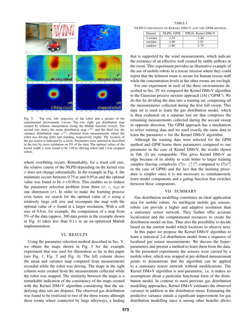
Fig. 5. Top row, left: trajectory of the robot and a picture of theexperimental environment 3-room. Top row, right: gas distribution mapcreated by trilinear interpolation (using the Matlab function trisurf). Thesecond row shows the mean distribution map r(k) and the third row thevariance distribution map v(k), obtained from measurements where therobot was driving (left) and standing, respectively (right). The location ofthe gas source is indicated by a circle. Parameters were selected as describedin the text by cross-validation on 5% of the data. The optimal values of thekernel width σ were found to be 1.05 m (driving robot) and 1.0 m (stoppedrobot).

where overfitting occurs. Remarkably, for a fixed cell size,the relative course of the NLPD depending on the kernel sizeσ does not change substantially. In the example in Fig. 4, theminimum occurs between 0.75 m and 0.95 m and the optimalvalue was found to be σ = 0.90 m. This enables us to reducethe parameter selection problem from three (σ, c, σΩ) toone dimension (σ). In order to make the learning processeven faster, we search for the optimal value of σ using arelatively large cell size and recompute the map with theoptimal value of σ found at a larger resolution. With a cellsize of 0.8 m, for example, the computation of a map from5% of the data (approx. 300 data points in the example shownin Fig. 4) takes less than 0.1 s in an un-optimized Matlabimplementation.

VI. RESULTS

Using the parameter selection method described in Sec. V,we obtain the maps shown in Fig. 5 for the exampleexperiment that was used for illustration so far in this paper(see Fig. 1, Fig. 2 and Fig. 4). The left column showsthe mean and variance map computed from measurementsrecorded while the robot was driving. The maps in the rightcolumn were created from the measurements collected whilethe robot was stopped. The similarity between the maps is aremarkable indication of the consistency of the maps createdwith the Kernel DM+V algorithm considering that the un-derlying data sets are disjunct. The observed gas distributionwas found to be restricted to two of the three rooms althoughthese rooms where connected by large alleyways, a finding

TABLE I

NLPD COMPARISON OF KERNEL DM+V AND THE GPM METHOD.

Dataset NLPD, GPM NPLD, Kernel DM+V

3-rooms -1.54 -1.44corridor -1.60 -1.81outdoor -1.80 -1.75

that is supported by the wind measurements, which indicatethe existence of an effective wall created by stable airflows inthe room. This experiment provides an illustrative example ofthe use of mobile robots in a rescue mission where they couldreport that the leftmost room is secure for human rescue staffwhile the concentration levels in the other rooms are too high.

For one experiment in each of the three environments de-scribed in Sec. IV we compared the Kernel DM+V algorithmto the Gaussian process mixture approach [16] (“GPM”). Wedo this by dividing the data into a training set, comprising allthe measurements collected during the first full sweep. Thisdata set is used to learn the gas distribution model, whichis then evaluated on a separate test set that comprises theremaining measurements collected during the second sweepin opposite direction. The GPM approach has a mechanismto select training data and we used exactly the same data tolearn the parameter σ for the Kernel DM+V algorithm.

Although the training data were selected for the GPMmethod and GPM learns three parameters compared to oneparameter in the case of Kernel DM+V, the results shownin Tab. (I) are comparable. This gives Kernel DM+V anedge because of its ability to scale better to larger trainingsamples (having complexity O[n · (σ

c )2] compared to O[n3]in the case of GPM) and the fact that the learning proce-dure is simpler since it is not necessary to simultaneouslylearn model components and a gating function that switchesbetween these components.

VII. SUMMARY

Gas distribution modelling constitutes an ideal applicationarea for mobile robots. As intelligent mobile gas sensors,robots can provide a higher and adaptive resolution thana stationary sensor network. They further offer accuratelocalization and the computational resources to create thedistribution model on-line. Thus also the possibility to decidebased on the current model which locations to observe next.

In this paper we propose the Kernel DM+V algorithm tolearn a statistical 2-d distribution model from a sequence oflocalized gas sensor measurements. We discuss the hyper-parameters and present a method to learn them from the data.In the presented experiments the sensors were carried by amobile robot, which was stopped at pre-defined measurementpoints to demonstrate that the algorithm can be appliedto a stationary sensor network without modifications. TheKernel DM+V algorithm is non-parametric, i.e. it makes noassumptions about a particular functional form of the distri-bution model. In contrast to most previous gas distributionmodelling approaches, Kernel DM+V estimates the observedvariance in addition to the distribution mean. Estimating thepredictive variance entails a significant improvement for gasdistribution modelling since it among other benefits allows

575

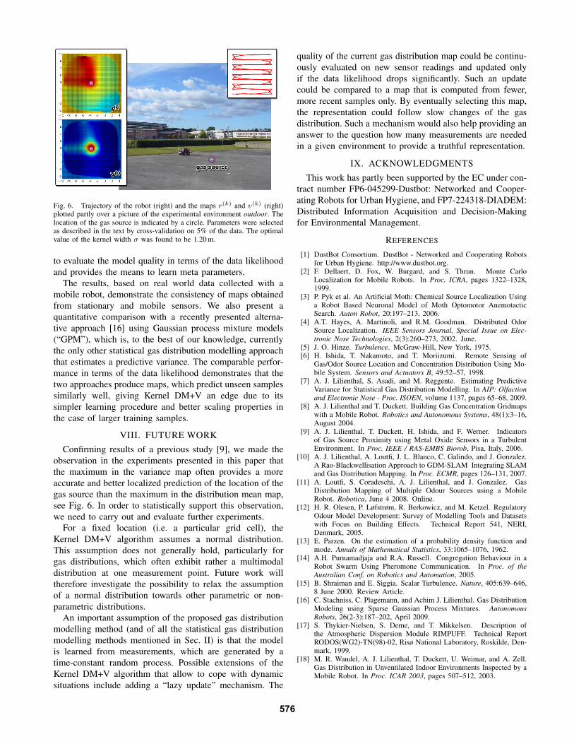
Fig. 6. Trajectory of the robot (right) and the maps r(k) and v(k) (right)plotted partly over a picture of the experimental environment outdoor. Thelocation of the gas source is indicated by a circle. Parameters were selectedas described in the text by cross-validation on 5% of the data. The optimalvalue of the kernel width σ was found to be 1.20 m.

to evaluate the model quality in terms of the data likelihoodand provides the means to learn meta parameters.

The results, based on real world data collected with amobile robot, demonstrate the consistency of maps obtainedfrom stationary and mobile sensors. We also present aquantitative comparison with a recently presented alterna-tive approach [16] using Gaussian process mixture models(“GPM”), which is, to the best of our knowledge, currentlythe only other statistical gas distribution modelling approachthat estimates a predictive variance. The comparable perfor-mance in terms of the data likelihood demonstrates that thetwo approaches produce maps, which predict unseen samplessimilarly well, giving Kernel DM+V an edge due to itssimpler learning procedure and better scaling properties inthe case of larger training samples.

VIII. FUTURE WORK

Confirming results of a previous study [9], we made theobservation in the experiments presented in this paper thatthe maximum in the variance map often provides a moreaccurate and better localized prediction of the location of thegas source than the maximum in the distribution mean map,see Fig. 6. In order to statistically support this observation,we need to carry out and evaluate further experiments.

For a fixed location (i.e. a particular grid cell), theKernel DM+V algorithm assumes a normal distribution.This assumption does not generally hold, particularly forgas distributions, which often exhibit rather a multimodaldistribution at one measurement point. Future work willtherefore investigate the possibility to relax the assumptionof a normal distribution towards other parametric or non-parametric distributions.

An important assumption of the proposed gas distributionmodelling method (and of all the statistical gas distributionmodelling methods mentioned in Sec. II) is that the modelis learned from measurements, which are generated by atime-constant random process. Possible extensions of theKernel DM+V algorithm that allow to cope with dynamicsituations include adding a “lazy update” mechanism. The

quality of the current gas distribution map could be continu-ously evaluated on new sensor readings and updated onlyif the data likelihood drops significantly. Such an updatecould be compared to a map that is computed from fewer,more recent samples only. By eventually selecting this map,the representation could follow slow changes of the gasdistribution. Such a mechanism would also help providing ananswer to the question how many measurements are neededin a given environment to provide a truthful representation.

IX. ACKNOWLEDGMENTS

This work has partly been supported by the EC under con-tract number FP6-045299-Dustbot: Networked and Cooper-ating Robots for Urban Hygiene, and FP7-224318-DIADEM:Distributed Information Acquisition and Decision-Makingfor Environmental Management.

REFERENCES

[1] DustBot Consortium. DustBot - Networked and Cooperating Robotsfor Urban Hygiene. http://www.dustbot.org.

[2] F. Dellaert, D. Fox, W. Burgard, and S. Thrun. Monte CarloLocalization for Mobile Robots. In Proc. ICRA, pages 1322–1328,1999.

[3] P. Pyk et al. An Artificial Moth: Chemical Source Localization Usinga Robot Based Neuronal Model of Moth Optomotor AnemotacticSearch. Auton Robot, 20:197–213, 2006.

[4] A.T. Hayes, A. Martinoli, and R.M. Goodman. Distributed OdorSource Localization. IEEE Sensors Journal, Special Issue on Elec-tronic Nose Technologies, 2(3):260–273, 2002. June.

[5] J. O. Hinze. Turbulence. McGraw-Hill, New York, 1975.[6] H. Ishida, T. Nakamoto, and T. Moriizumi. Remote Sensing of

Gas/Odor Source Location and Concentration Distribution Using Mo-bile System. Sensors and Actuators B, 49:52–57, 1998.

[7] A. J. Lilienthal, S. Asadi, and M. Reggente. Estimating PredictiveVariance for Statistical Gas Distribution Modelling. In AIP: Olfactionand Electronic Nose - Proc. ISOEN, volume 1137, pages 65–68, 2009.

[8] A. J. Lilienthal and T. Duckett. Building Gas Concentration Gridmapswith a Mobile Robot. Robotics and Autonomous Systems, 48(1):3–16,August 2004.

[9] A. J. Lilienthal, T. Duckett, H. Ishida, and F. Werner. Indicatorsof Gas Source Proximity using Metal Oxide Sensors in a TurbulentEnvironment. In Proc. IEEE / RAS-EMBS Biorob, Pisa, Italy, 2006.

[10] A. J. Lilienthal, A. Loutfi, J. L. Blanco, C. Galindo, and J. Gonzalez.A Rao-Blackwellisation Approach to GDM-SLAM Integrating SLAMand Gas Distribution Mapping. In Proc. ECMR, pages 126–131, 2007.

[11] A. Loutfi, S. Coradeschi, A. J. Lilienthal, and J. Gonzalez. GasDistribution Mapping of Multiple Odour Sources using a MobileRobot. Robotica, June 4 2008. Online.

[12] H. R. Olesen, P. Løfstrøm, R. Berkowicz, and M. Ketzel. RegulatoryOdour Model Development: Survey of Modelling Tools and Datasetswith Focus on Building Effects. Technical Report 541, NERI,Denmark, 2005.

[13] E. Parzen. On the estimation of a probability density function andmode. Annals of Mathematical Statistics, 33:1065–1076, 1962.

[14] A.H. Purnamadjaja and R.A. Russell. Congregation Behaviour in aRobot Swarm Using Pheromone Communication. In Proc. of theAustralian Conf. on Robotics and Automation, 2005.

[15] B. Shraiman and E. Siggia. Scalar Turbulence. Nature, 405:639–646,8 June 2000. Review Article.

[16] C. Stachniss, C. Plagemann, and Achim J. Lilienthal. Gas DistributionModeling using Sparse Gaussian Process Mixtures. AutonomousRobots, 26(2-3):187–202, April 2009.

[17] S. Thykier-Nielsen, S. Deme, and T. Mikkelsen. Description ofthe Atmospheric Dispersion Module RIMPUFF. Technical ReportRODOS(WG2)-TN(98)-02, Risø National Laboratory, Roskilde, Den-mark, 1999.

[18] M. R. Wandel, A. J. Lilienthal, T. Duckett, U. Weimar, and A. Zell.Gas Distribution in Unventilated Indoor Environments Inspected by aMobile Robot. In Proc. ICAR 2003, pages 507–512, 2003.

576