A statistical 3-D pattern processing method for computer-aided detection of polyps in CT colonography

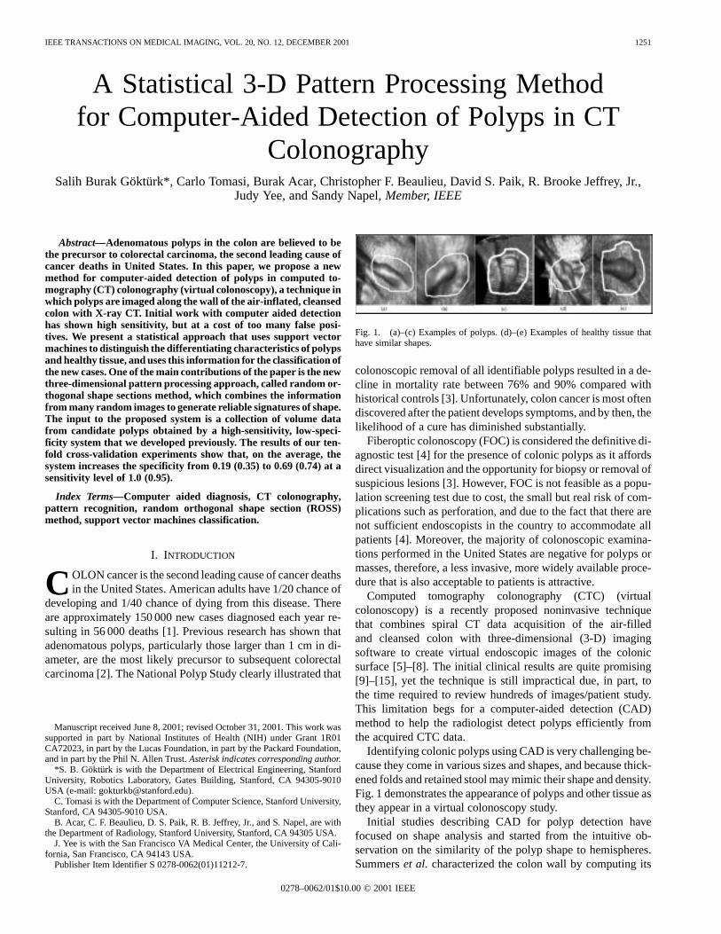
IEEE TRANSACTIONS ON MEDICAL IMAGING, VOL. 20, NO. 12, DECEMBER 2001 1251

A Statistical 3-D Pattern Processing Methodfor Computer-Aided Detection of Polyps in CT

ColonographySalih Burak Göktürk*, Carlo Tomasi, Burak Acar, Christopher F. Beaulieu, David S. Paik, R. Brooke Jeffrey, Jr.,

Judy Yee, and Sandy Napel, Member, IEEE

Abstract—Adenomatous polyps in the colon are believed to bethe precursor to colorectal carcinoma, the second leading cause ofcancer deaths in United States. In this paper, we propose a newmethod for computer-aided detection of polyps in computed to-mography (CT) colonography (virtual colonoscopy), a technique inwhich polyps are imaged along the wall of the air-inflated, cleansedcolon with X-ray CT. Initial work with computer aided detectionhas shown high sensitivity, but at a cost of too many false posi-tives. We present a statistical approach that uses support vectormachines to distinguish the differentiating characteristics of polypsand healthy tissue, and uses this information for the classification ofthe new cases. One of the main contributions of the paper is the newthree-dimensional pattern processing approach, called random or-thogonal shape sections method, which combines the informationfrom many random images to generate reliable signatures of shape.The input to the proposed system is a collection of volume datafrom candidate polyps obtained by a high-sensitivity, low-speci-ficity system that we developed previously. The results of our ten-fold cross-validation experiments show that, on the average, thesystem increases the specificity from 0.19 (0.35) to 0.69 (0.74) at asensitivity level of 1.0 (0.95).

Index Terms—Computer aided diagnosis, CT colonography,pattern recognition, random orthogonal shape section (ROSS)method, support vector machines classification.

I. INTRODUCTION

COLON cancer is the second leading cause of cancer deathsin the United States. American adults have 1/20 chance of

developing and 1/40 chance of dying from this disease. Thereare approximately 150 000 new cases diagnosed each year re-sulting in 56 000 deaths [1]. Previous research has shown thatadenomatous polyps, particularly those larger than 1 cm in di-ameter, are the most likely precursor to subsequent colorectalcarcinoma [2]. The National Polyp Study clearly illustrated that

Manuscript received June 8, 2001; revised October 31, 2001. This work wassupported in part by National Institutes of Health (NIH) under Grant 1R01CA72023, in part by the Lucas Foundation, in part by the Packard Foundation,and in part by the Phil N. Allen Trust.Asterisk indicates corresponding author.

*S. B. Göktürk is with the Department of Electrical Engineering, StanfordUniversity, Robotics Laboratory, Gates Building, Stanford, CA 94305-9010USA (e-mail: [email protected]).

C. Tomasi is with the Department of Computer Science, Stanford University,Stanford, CA 94305-9010 USA.

B. Acar, C. F. Beaulieu, D. S. Paik, R. B. Jeffrey, Jr., and S. Napel, are withthe Department of Radiology, Stanford University, Stanford, CA 94305 USA.

J. Yee is with the San Francisco VA Medical Center, the University of Cali-fornia, San Francisco, CA 94143 USA.

Publisher Item Identifier S 0278-0062(01)11212-7.

Fig. 1. (a)–(c) Examples of polyps. (d)–(e) Examples of healthy tissue thathave similar shapes.

colonoscopic removal of all identifiable polyps resulted in a de-cline in mortality rate between 76% and 90% compared withhistorical controls [3]. Unfortunately, colon cancer is most oftendiscovered after the patient develops symptoms, and by then, thelikelihood of a cure has diminished substantially.

Fiberoptic colonoscopy (FOC) is considered the definitive di-agnostic test [4] for the presence of colonic polyps as it affordsdirect visualization and the opportunity for biopsy or removal ofsuspicious lesions [3]. However, FOC is not feasible as a popu-lation screening test due to cost, the small but real risk of com-plications such as perforation, and due to the fact that there arenot sufficient endoscopists in the country to accommodate allpatients [4]. Moreover, the majority of colonoscopic examina-tions performed in the United States are negative for polyps ormasses, therefore, a less invasive, more widely available proce-dure that is also acceptable to patients is attractive.

Computed tomography colonography (CTC) (virtualcolonoscopy) is a recently proposed noninvasive techniquethat combines spiral CT data acquisition of the air-filledand cleansed colon with three-dimensional (3-D) imagingsoftware to create virtual endoscopic images of the colonicsurface [5]–[8]. The initial clinical results are quite promising[9]–[15], yet the technique is still impractical due, in part, tothe time required to review hundreds of images/patient study.This limitation begs for a computer-aided detection (CAD)method to help the radiologist detect polyps efficiently fromthe acquired CTC data.

Identifying colonic polyps using CAD is very challenging be-cause they come in various sizes and shapes, and because thick-ened folds and retained stool may mimic their shape and density.Fig. 1 demonstrates the appearance of polyps and other tissue asthey appear in a virtual colonoscopy study.

Initial studies describing CAD for polyp detection havefocused on shape analysis and started from the intuitive ob-servation on the similarity of the polyp shape to hemispheres.Summerset al. characterized the colon wall by computing its

0278–0062/01$10.00 © 2001 IEEE

1252 IEEE TRANSACTIONS ON MEDICAL IMAGING, VOL. 20, NO. 12, DECEMBER 2001

minimum, maximum, mean, and Gaussian curvatures [16].Following discrimination of polypoid shapes by their principalminimum and maximum curvatures, more restrictive criteriasuch as sphericity measures are applied in order to eliminatenonspherical shapes. In [17], Yoshidaet al. use topologicalshape of vicinity of each voxel, in addition with a measurefor the shape curvedness to distinguish polyps from healthytissue. Gokturk and Tomasi designed a method based on theobservation that the bounding surfaces of polyps are usuallynot exact spheres, but are often complex surfaces composed ofsmall, approximately spherical patches [18]. In this method, asphere is fit locally to the isodensity surface passing throughevery CT voxel in the wall region. Groups of voxels that origi-nate densely populated nearby sphere centers are considered aspolyp candidates. Obviously, the clusters of the sphere centersare more dense when the underlying shape is a sphere or ahemisphere. In [19] and [20], Paiket al. introduced a methodbased on the concept that normals to the colon surface willintersect with neighboring normals depending on the localcurvature features of the colon. Their work uses the observationthat polyps have 3-D shape features that change rapidly inmany directions, so that normals to the surface tend to intersectin a concentrated area. By contrast, haustral folds change theirshape rapidly when sampled transversely, resulting in conver-gence of normals, but change shape very slowly when sampledlongitudinally. As a result, the method detects the polyps bygiving the shapes a score based on the number of intersectingnormal vectors. This score is higher in hemispherical polypscompared with folds.

While these methods have demonstrated promising sensi-tivity, they can be considered more as polyp candidate detectorsthan polyp detectors because of their large number of falsepositive detections. These methods have observed that polypshave spherical shapes, and provided different measures ofsphericity. However, polyps span a large variety of shapes, andfitting spheres alone is not an accurate measure. This paperpresents a statistical method to differentiate between polypsand normal tissue. Our new 3-D pattern processing method,called random orthogonal shape section (ROSS) methodgenerates shape-signatures for small candidate volumes, whichmight be obtained by one of the above mentioned methods,and then feeds these signatures to a support vector machines(SVM) classifier for the final diagnosis of the volume. By usingstatistical learning, the different characteristics of polyps andnormal tissue are automatically extracted from the data.

The paper is organized as follows: Section II describes ourproposed technique, explaining both the pattern processing andthe SVM classifier, and our evaluation methods. Section IIIpresents our results, followed by discussion in Section IV andconclusions in Section V.

II. M ETHODS

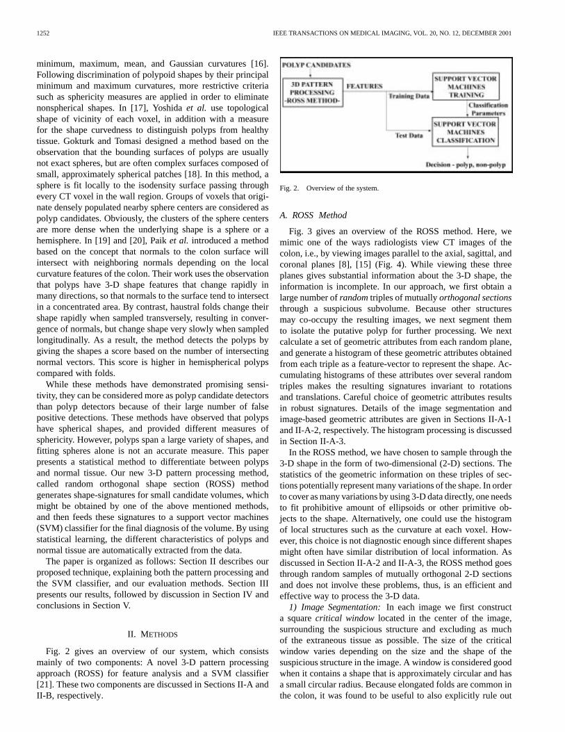
Fig. 2 gives an overview of our system, which consistsmainly of two components: A novel 3-D pattern processingapproach (ROSS) for feature analysis and a SVM classifier[21]. These two components are discussed in Sections II-A andII-B, respectively.

Fig. 2. Overview of the system.

A. ROSS Method

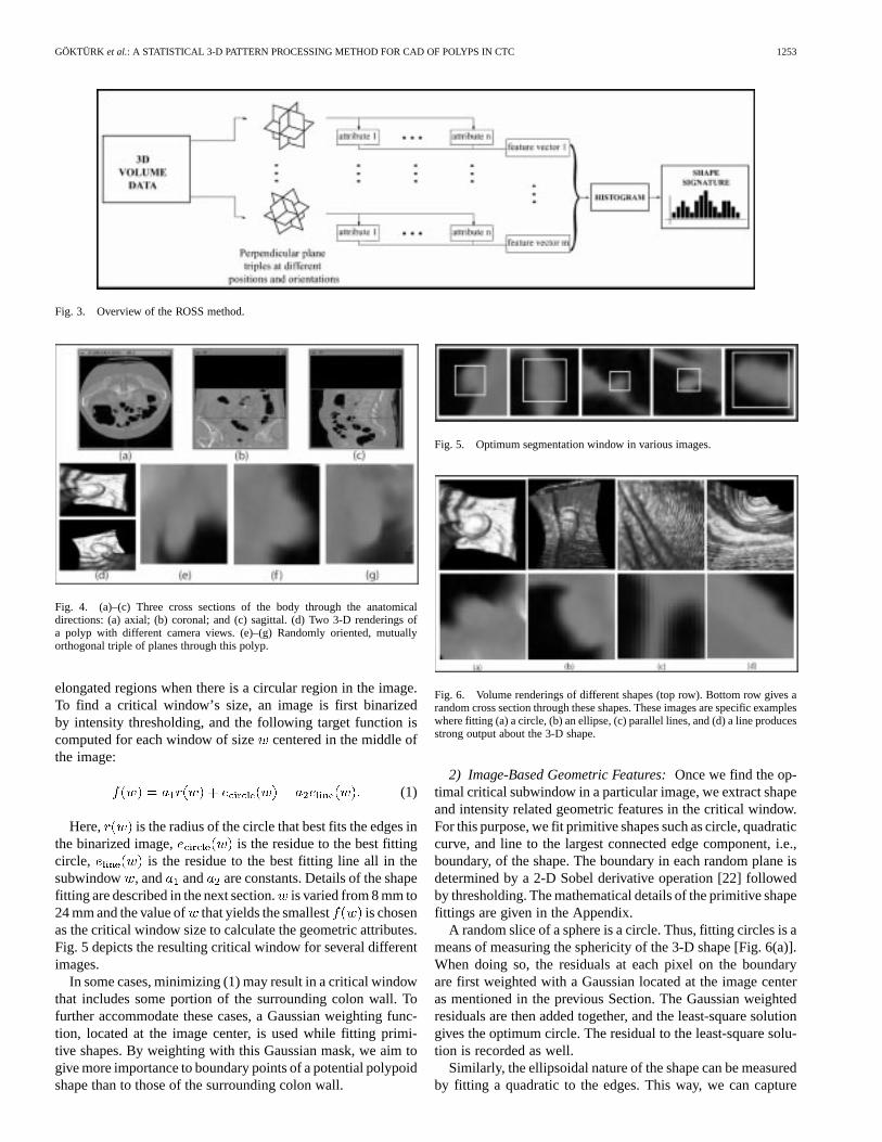
Fig. 3 gives an overview of the ROSS method. Here, wemimic one of the ways radiologists view CT images of thecolon, i.e., by viewing images parallel to the axial, sagittal, andcoronal planes [8], [15] (Fig. 4). While viewing these threeplanes gives substantial information about the 3-D shape, theinformation is incomplete. In our approach, we first obtain alarge number ofrandomtriples of mutuallyorthogonal sectionsthrough a suspicious subvolume. Because other structuresmay co-occupy the resulting images, we next segment themto isolate the putative polyp for further processing. We nextcalculate a set of geometric attributes from each random plane,and generate a histogram of these geometric attributes obtainedfrom each triple as a feature-vector to represent the shape. Ac-cumulating histograms of these attributes over several randomtriples makes the resulting signatures invariant to rotationsand translations. Careful choice of geometric attributes resultsin robust signatures. Details of the image segmentation andimage-based geometric attributes are given in Sections II-A-1and II-A-2, respectively. The histogram processing is discussedin Section II-A-3.

In the ROSS method, we have chosen to sample through the3-D shape in the form of two-dimensional (2-D) sections. Thestatistics of the geometric information on these triples of sec-tions potentially represent many variations of the shape. In orderto cover as many variations by using 3-D data directly, one needsto fit prohibitive amount of ellipsoids or other primitive ob-jects to the shape. Alternatively, one could use the histogramof local structures such as the curvature at each voxel. How-ever, this choice is not diagnostic enough since different shapesmight often have similar distribution of local information. Asdiscussed in Section II-A-2 and II-A-3, the ROSS method goesthrough random samples of mutually orthogonal 2-D sectionsand does not involve these problems, thus, is an efficient andeffective way to process the 3-D data.

1) Image Segmentation:In each image we first constructa squarecritical window located in the center of the image,surrounding the suspicious structure and excluding as muchof the extraneous tissue as possible. The size of the criticalwindow varies depending on the size and the shape of thesuspicious structure in the image. A window is considered goodwhen it contains a shape that is approximately circular and hasa small circular radius. Because elongated folds are common inthe colon, it was found to be useful to also explicitly rule out

GÖKTÜRK et al.: A STATISTICAL 3-D PATTERN PROCESSING METHOD FOR CAD OF POLYPS IN CTC 1253

Fig. 3. Overview of the ROSS method.

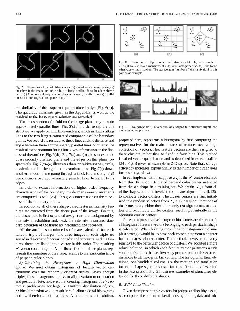
Fig. 4. (a)–(c) Three cross sections of the body through the anatomicaldirections: (a) axial; (b) coronal; and (c) sagittal. (d) Two 3-D renderings ofa polyp with different camera views. (e)–(g) Randomly oriented, mutuallyorthogonal triple of planes through this polyp.

elongated regions when there is a circular region in the image.To find a critical window’s size, an image is first binarizedby intensity thresholding, and the following target function iscomputed for each window of size centered in the middle ofthe image:

(1)

Here, is the radius of the circle that best fits the edges inthe binarized image, is the residue to the best fittingcircle, is the residue to the best fitting line all in thesubwindow , and and are constants. Details of the shapefitting are described in the next section.is varied from 8 mm to24 mm and the value of that yields the smallest is chosenas the critical window size to calculate the geometric attributes.Fig. 5 depicts the resulting critical window for several differentimages.

In some cases, minimizing (1) may result in a critical windowthat includes some portion of the surrounding colon wall. Tofurther accommodate these cases, a Gaussian weighting func-tion, located at the image center, is used while fitting primi-tive shapes. By weighting with this Gaussian mask, we aim togive more importance to boundary points of a potential polypoidshape than to those of the surrounding colon wall.

Fig. 5. Optimum segmentation window in various images.

Fig. 6. Volume renderings of different shapes (top row). Bottom row gives arandom cross section through these shapes. These images are specific exampleswhere fitting (a) a circle, (b) an ellipse, (c) parallel lines, and (d) a line producesstrong output about the 3-D shape.

2) Image-Based Geometric Features:Once we find the op-timal critical subwindow in a particular image, we extract shapeand intensity related geometric features in the critical window.For this purpose, we fit primitive shapes such as circle, quadraticcurve, and line to the largest connected edge component, i.e.,boundary, of the shape. The boundary in each random plane isdetermined by a 2-D Sobel derivative operation [22] followedby thresholding. The mathematical details of the primitive shapefittings are given in the Appendix.

A random slice of a sphere is a circle. Thus, fitting circles is ameans of measuring the sphericity of the 3-D shape [Fig. 6(a)].When doing so, the residuals at each pixel on the boundaryare first weighted with a Gaussian located at the image centeras mentioned in the previous Section. The Gaussian weightedresiduals are then added together, and the least-square solutiongives the optimum circle. The residual to the least-square solu-tion is recorded as well.

Similarly, the ellipsoidal nature of the shape can be measuredby fitting a quadratic to the edges. This way, we can capture


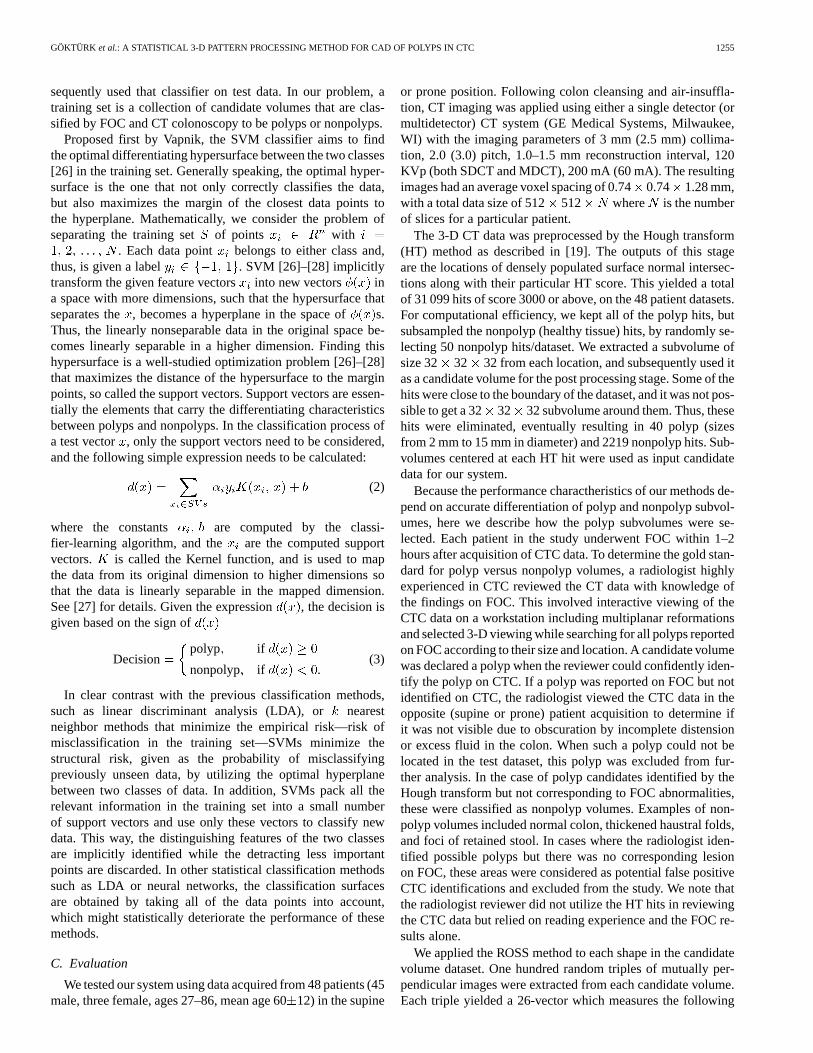
Fig. 7. Illustration of the primitive shapes: (a) a randomly oriented plane; (b)the edges in the image; (c)–(e) circle, quadratic, and line fit to the edges shownin (b). (f) Another randomly oriented plane with nearly parallel lines (g) parallellines fit to the edges of the plane in (f).

the similarity of the shape to a pedunculated polyp [Fig. 6(b)].The quadratic invariants given in the Appendix, as well as theresidual to the least-square solution are recorded.

The cross section of a fold on the image plane may containapproximately parallel lines [Fig. 6(c)]. In order to capture thisstructure, we apply parallel lines analysis, which includes fittinglines to the two largest connected components of the boundarypoints. We record the residual to these lines and the distance andangle between these approximately parallel lines. Similarly, theresidual to the optimum fitting line gives information on the flat-ness of the surface [Fig. 6(d)]. Fig. 7(a) and (b) gives an exampleof a randomly oriented plane and the edges on this plane, re-spectively. Fig. 7(c)–(e) illustrates three primitive shapes, circle,quadratic and line being fit to this random plane. Fig. 7(f) showsanother random plane going through a thick fold and Fig. 7(g)demonstrates two approximately parallel lines being fit to itsedges.

In order to extract information on higher order frequencycharacteristics of the boundary, third-order moment invariantsare computed as well [23]. This gives information on the curvi-ness of the boundary points.

In addition to all of these shape-based features, intensity fea-tures are extracted from the tissue part of the image. For this,the tissue part is first separated away from the background byintensity thresholding and, next, the intensity mean and stan-dard deviation of the tissue are calculated and recorded.

All the attributes mentioned so far are calculated for eachrandom triple of images. The three images in each triple aresorted in the order of increasing radius of curvature, and the fea-tures above are listed into a vector in this order. The resulting

-vector containing the attributes from the three planes rep-resents the signature of the shape, relative to that particular tripleof perpendicular planes.

3) Obtaining the Histograms in High DimensionalSpace: We next obtain histograms of feature vector dis-tributions over the randomly oriented triples. Given enoughtriples, these histograms are essentially invariant to orientationand position. Note, however, that creating histograms of-vec-tors is problematic for large . Uniform distribution of, say,

bins/dimension would result in -dimensional histogramsand is, therefore, not tractable. A more efficient solution,

Fig. 8. Illustration of high dimensional histogram bins by an example in2-D. (a) Data in two dimensions. (b) Uniform histogram bins. (c) Bins foundwhen clustering is applied. The storage gain (number of bins) is fivefold in thisparticular example.

Fig. 9. Two polyps (left), a very similarly shaped fold structure (right), andtheir signatures (center).

proposed here, represents a histogram by first computing therepresentatives for the main clusters of features over a largecollection of vectors. New feature vectors are then assigned tothese clusters, rather than to fixed uniform bins. This methodis called vector quantization and is described in more detail in[24]. Fig. 8 gives an example in 2-D space. Note that, storageefficiency increases exponentially as the number of dimensionsincrease beyond two.

In our implementation, suppose is the -vector obtainedfrom the th random triple of perpendicular planes extractedfrom the th shape in a training set. We obtain s from allof the shapes, and then invoke the-means algorithm [24], [25]to compute vector clusters. The cluster centers are first initial-ized to a random selection from s. Subsequent iterations ofthe -means algorithm then alternately reassign vectors to clus-ters and recompute cluster centers, resulting eventually in theoptimum cluster centers.

Once the representative histogram bin centers are determined,a histogram of feature vectors belonging to each particular shapeis calculated. When forming these feature histograms, the sim-plest strategy would be to have each vector increment a counterfor the nearest cluster center. This method, however, is overlysensitive to the particular choice of clusters. We adopted a morerobust solution, in which each feature vector partitions a unitvote into fractions that are inversely proportional to the vector’sdistances to all histogram bin centers. The histograms, thus, ob-tained, one/candidate volume, are the rotation and translationinvariant shape signatures used for classification as describedin the next section. Fig. 9 illustrates examples of signatures ob-tained for three different shapes.

B. SVM Classification

Given the representative vectors for polyps and healthy tissue,we computed the optimum classifier using training data and sub-


sequently used that classifier on test data. In our problem, atraining set is a collection of candidate volumes that are clas-sified by FOC and CT colonoscopy to be polyps or nonpolyps.

Proposed first by Vapnik, the SVM classifier aims to findthe optimal differentiating hypersurface between the two classes[26] in the training set. Generally speaking, the optimal hyper-surface is the one that not only correctly classifies the data,but also maximizes the margin of the closest data points tothe hyperplane. Mathematically, we consider the problem ofseparating the training set of points with

. Each data point belongs to either class and,thus, is given a label . SVM [26]–[28] implicitlytransform the given feature vectorsinto new vectors ina space with more dimensions, such that the hypersurface thatseparates the, becomes a hyperplane in the space of s.Thus, the linearly nonseparable data in the original space be-comes linearly separable in a higher dimension. Finding thishypersurface is a well-studied optimization problem [26]–[28]that maximizes the distance of the hypersurface to the marginpoints, so called the support vectors. Support vectors are essen-tially the elements that carry the differentiating characteristicsbetween polyps and nonpolyps. In the classification process ofa test vector , only the support vectors need to be considered,and the following simple expression needs to be calculated:

(2)

where the constants are computed by the classi-fier-learning algorithm, and the are the computed supportvectors. is called the Kernel function, and is used to mapthe data from its original dimension to higher dimensions sothat the data is linearly separable in the mapped dimension.See [27] for details. Given the expression , the decision isgiven based on the sign of

Decisionpolyp if

nonpolyp if .(3)

In clear contrast with the previous classification methods,such as linear discriminant analysis (LDA), or nearestneighbor methods that minimize the empirical risk—risk ofmisclassification in the training set—SVMs minimize thestructural risk, given as the probability of misclassifyingpreviously unseen data, by utilizing the optimal hyperplanebetween two classes of data. In addition, SVMs pack all therelevant information in the training set into a small numberof support vectors and use only these vectors to classify newdata. This way, the distinguishing features of the two classesare implicitly identified while the detracting less importantpoints are discarded. In other statistical classification methodssuch as LDA or neural networks, the classification surfacesare obtained by taking all of the data points into account,which might statistically deteriorate the performance of thesemethods.

C. Evaluation

We tested our system using data acquired from 48 patients (45male, three female, ages 27–86, mean age 6012) in the supine

or prone position. Following colon cleansing and air-insuffla-tion, CT imaging was applied using either a single detector (ormultidetector) CT system (GE Medical Systems, Milwaukee,WI) with the imaging parameters of 3 mm (2.5 mm) collima-tion, 2.0 (3.0) pitch, 1.0–1.5 mm reconstruction interval, 120KVp (both SDCT and MDCT), 200 mA (60 mA). The resultingimages had an average voxel spacing of 0.740.74 1.28 mm,with a total data size of 512 512 where is the numberof slices for a particular patient.

The 3-D CT data was preprocessed by the Hough transform(HT) method as described in [19]. The outputs of this stageare the locations of densely populated surface normal intersec-tions along with their particular HT score. This yielded a totalof 31 099 hits of score 3000 or above, on the 48 patient datasets.For computational efficiency, we kept all of the polyp hits, butsubsampled the nonpolyp (healthy tissue) hits, by randomly se-lecting 50 nonpolyp hits/dataset. We extracted a subvolume ofsize 32 32 32 from each location, and subsequently used itas a candidate volume for the post processing stage. Some of thehits were close to the boundary of the dataset, and it was not pos-sible to get a 32 32 32 subvolume around them. Thus, thesehits were eliminated, eventually resulting in 40 polyp (sizesfrom 2 mm to 15 mm in diameter) and 2219 nonpolyp hits. Sub-volumes centered at each HT hit were used as input candidatedata for our system.

Because the performance charactheristics of our methods de-pend on accurate differentiation of polyp and nonpolyp subvol-umes, here we describe how the polyp subvolumes were se-lected. Each patient in the study underwent FOC within 1–2hours after acquisition of CTC data. To determine the gold stan-dard for polyp versus nonpolyp volumes, a radiologist highlyexperienced in CTC reviewed the CT data with knowledge ofthe findings on FOC. This involved interactive viewing of theCTC data on a workstation including multiplanar reformationsand selected 3-D viewing while searching for all polyps reportedon FOC according to their size and location. A candidate volumewas declared a polyp when the reviewer could confidently iden-tify the polyp on CTC. If a polyp was reported on FOC but notidentified on CTC, the radiologist viewed the CTC data in theopposite (supine or prone) patient acquisition to determine ifit was not visible due to obscuration by incomplete distensionor excess fluid in the colon. When such a polyp could not belocated in the test dataset, this polyp was excluded from fur-ther analysis. In the case of polyp candidates identified by theHough transform but not corresponding to FOC abnormalities,these were classified as nonpolyp volumes. Examples of non-polyp volumes included normal colon, thickened haustral folds,and foci of retained stool. In cases where the radiologist iden-tified possible polyps but there was no corresponding lesionon FOC, these areas were considered as potential false positiveCTC identifications and excluded from the study. We note thatthe radiologist reviewer did not utilize the HT hits in reviewingthe CTC data but relied on reading experience and the FOC re-sults alone.

We applied the ROSS method to each shape in the candidatevolume dataset. One hundred random triples of mutually per-pendicular images were extracted from each candidate volume.Each triple yielded a 26-vector which measures the following


features on the random planes: Best-fit circle’s radius, residueto the best-fit circle, line and quadratic curve, quadratic shape in-variants, moment invariants, angle, and distance between nearlyparallel lines (if there are such pair of lines in the image), andtotal residue to line fit in the pair of parallel lines. The distri-bution of information belonging to the 26-vector of 100 triplesis estimated by high dimensional histograms as described inSection II-A-3. The -means algorithm is executed to obtain45-vector centers which are then used as histogram bin centers.Therefore, the high dimensional histograms obtained by vectorquantization resulted in a 45-dimensional vector to representeach particular candidate volume. These vectors were used bythe SVM classification algorithm with exponential radial basisfunctions as kernel functions [29].

We conducted a tenfold cross-validation experiment to eval-uate our system. First, we randomly divided the candidate vol-umes into ten uniformly distributed sets of ten polyps (withrepetitions, average overlap between sets is 1.8 polyps, max-imum overlap is four polyps) and 221 or 222 nonpolyps (healthytissue, without repetitions). In each of these ten experiments,one set was used as the test set, and the remaining 30 polypsand 1997 (1998) nonpolyps as training set. In our analysis, wewill refer to sensitivity as the fraction of detected polyps, andto specificity as the fraction of detected normal tissue volumesamong the nonpolyp locations.

To examine the tradeoff between the sensitivity and speci-ficity more quantitatively, we substituted zero-crossing sign in(3), with a level crossing (SVM threshold,). As the level isdecreased, more true polyps are detected, but at a cost of morefalse positives. In this way, for any input collection of polypsand nonpolyps, we can obtain a receiver operating characteristic(ROC) curve [sensitivity versus (1-specificity) curve]. Similarly,the HT method uses a threshold,, that denotes the minimumscore necessary to declare a candidate volume to be a polyp.Thus, by varying , one can also construct an ROC curve.

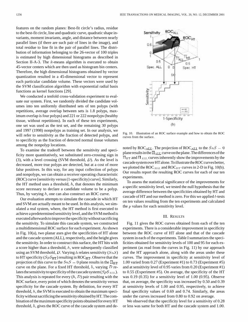
Our evaluation attempts to simulate the cascade in which HTand SVM are actually meant to be used. In this analysis, we sim-ulated a real system, where, the HT method is first executed toachieve a predeterminedsensitivity level, and the SVMmethod isexecutedafterwardsto improvethespecificitywithoutsacrificingthe sensitivity. To simulate this cascade system, we constructeda multidimensional ROC surface for each experiment. As shownin Fig. 10(a), two planar axes give the specificities of HT aloneand the cascade system (ALL), respectively, and the height givesthe sensitivity. In order to construct this surface, the HT hits witha score higher than a threshold,, were subsequently classifiedusing an SVM threshold, . Varying relates sensitivity ( )to HT specificity ( ) resulting in ROC . Observe that theprojection of this curve to the plane results in thecurve on the plane. For a fixed HT threshold,, varying re-latesthesensitivitytospecificityofthecascadesystem( ).This analysis is repeated for every (, ) pair resulting with theROC surface, every point of which denotes the sensitivity versusspecificity for the cascade system. By definition, for every HTthreshold, , the SVM is executed to obtain the maximum speci-ficitywithoutsacrificingthesensitivityobtainedbyHT.Thecom-binationof themaximumspecificitypointsobtainedforeveryHTthreshold, , gives the ROC curve of the cascade system and de-

Fig. 10. Illustration of an ROC surface example and how to obtain the ROCcurves from the surface.

noted by ROC . The projection of ROC to theplaneresults inthe curveontheplane.Thedifferencesofthe

and curves inherently show the improvements by thecascadesystemoverHTalone.ToillustratetheROCcurvesbetter,we plotted the ROC and ROC curves in 2-D in Fig. 10(b).Our results report the resulting ROC curves for each of our tenexperiments.

To assess the statistical significance of the improvements fora specific sensitivity level, we tested the null hypothesis that theaverage difference between the specificities obtained by HT andcascade of HT and our method is zero. For this we applied-testson ten values resulting from the ten experiments and calculatedthe values for each sensitivity level.

III. RESULTS

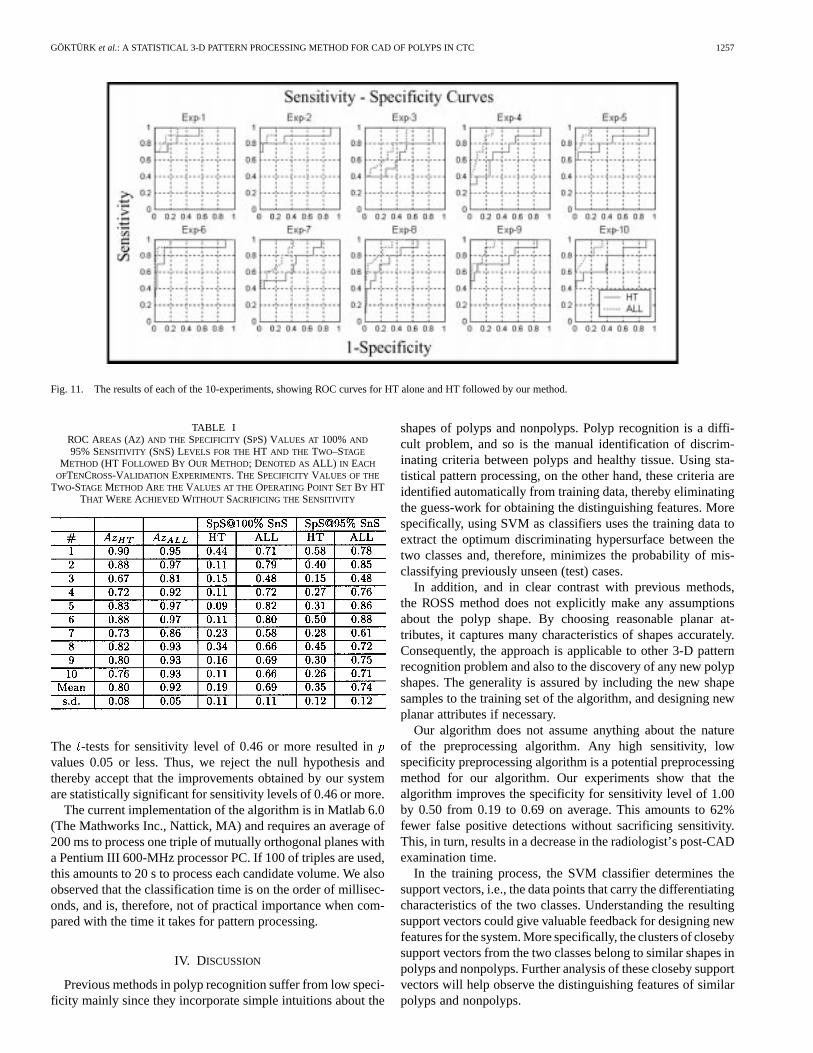
Fig. 11 gives the ROC curves obtained from each of the tenexperiments. There is a considerable improvement in specificitybetween the ROC curve of HT alone and that of the cascadesystem in each of the experiments. Table I summarizes the speci-ficities obtained for sensitivity levels of 100 and 95 for each ex-periment (as read from the curves in Fig. 11) by our approachand the HT approach alone, along with the areas under thesecurves. The improvement in specificity at sensitivity level of1.00 varied from 0.27 (Experiment #1) to 0.73 (Experiment #5)and at sensitivity level of 0.95 varies from 0.20 (Experiment #1)to 0.55 (Experiment #5). On average, the specificity of the HTwas 0.19 (0.35) for a sensitivity level of 1.00 (0.95). Observethat, on average, the specificity was increased by 0.50 and 0.39at sensitivity levels of 1.00 and 0.95, respectively, to achievefinal specificity values of 0.69 and 0.74. Similarly, the areasunder the curves increased from 0.80 to 0.92 on average.

We observed that the specificity level for a sensitivity of 0.28or less was same for both HT and the cascade system and 1.00.


Fig. 11. The results of each of the 10-experiments, showing ROC curves for HT alone and HT followed by our method.

TABLE IROC AREAS (AZ) AND THE SPECIFICITY (SPS) VALUES AT 100%AND

95% SENSITIVITY (SNS) LEVELS FOR THEHT AND THE TWO–STAGE

METHOD (HT FOLLOWED BY OUR METHOD; DENOTED ASALL) IN EACH

OFTENCROSS-VALIDATION EXPERIMENTS. THE SPECIFICITY VALUES OF THE

TWO-STAGE METHOD ARE THEVALUES AT THE OPERATINGPOINT SET BY HTTHAT WERE ACHIEVED WITHOUT SACRIFICING THE SENSITIVITY

The -tests for sensitivity level of 0.46 or more resulted invalues 0.05 or less. Thus, we reject the null hypothesis andthereby accept that the improvements obtained by our systemare statistically significant for sensitivity levels of 0.46 or more.

The current implementation of the algorithm is in Matlab 6.0(The Mathworks Inc., Nattick, MA) and requires an average of200 ms to process one triple of mutually orthogonal planes witha Pentium III 600-MHz processor PC. If 100 of triples are used,this amounts to 20 s to process each candidate volume. We alsoobserved that the classification time is on the order of millisec-onds, and is, therefore, not of practical importance when com-pared with the time it takes for pattern processing.

IV. DISCUSSION

Previous methods in polyp recognition suffer from low speci-ficity mainly since they incorporate simple intuitions about the

shapes of polyps and nonpolyps. Polyp recognition is a diffi-cult problem, and so is the manual identification of discrim-inating criteria between polyps and healthy tissue. Using sta-tistical pattern processing, on the other hand, these criteria areidentified automatically from training data, thereby eliminatingthe guess-work for obtaining the distinguishing features. Morespecifically, using SVM as classifiers uses the training data toextract the optimum discriminating hypersurface between thetwo classes and, therefore, minimizes the probability of mis-classifying previously unseen (test) cases.

In addition, and in clear contrast with previous methods,the ROSS method does not explicitly make any assumptionsabout the polyp shape. By choosing reasonable planar at-tributes, it captures many characteristics of shapes accurately.Consequently, the approach is applicable to other 3-D patternrecognition problem and also to the discovery of any new polypshapes. The generality is assured by including the new shapesamples to the training set of the algorithm, and designing newplanar attributes if necessary.

Our algorithm does not assume anything about the natureof the preprocessing algorithm. Any high sensitivity, lowspecificity preprocessing algorithm is a potential preprocessingmethod for our algorithm. Our experiments show that thealgorithm improves the specificity for sensitivity level of 1.00by 0.50 from 0.19 to 0.69 on average. This amounts to 62%fewer false positive detections without sacrificing sensitivity.This, in turn, results in a decrease in the radiologist’s post-CADexamination time.

In the training process, the SVM classifier determines thesupport vectors, i.e., the data points that carry the differentiatingcharacteristics of the two classes. Understanding the resultingsupport vectors could give valuable feedback for designing newfeatures for the system. More specifically, the clusters of closebysupport vectors from the two classes belong to similar shapes inpolyps and nonpolyps. Further analysis of these closeby supportvectors will help observe the distinguishing features of similarpolyps and nonpolyps.


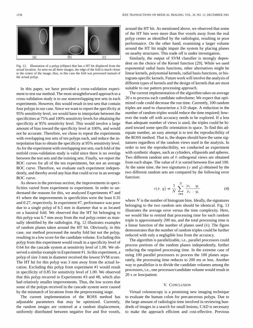
Fig. 12. Illustration of a polyp (ellipse) that has a HT hit displaced from theactual location. As seen on all three images, the edge of the fold is much closerto the center of the image; thus, in this case the fold was processed instead ofthe actual polyp.

In this paper, we have provided a cross-validation experi-ment to test our method. The most straightforward approach to across-validation study is to use nonoverlapping test sets in eachexperiments. However, this would result in test sets that containfour polyps in our case. Since we want to report the specificity at95% sensitivity level, we would have to interpolate between thespecificities at 75% and 100% sensitivity levels for obtaining thespecificity at 95% sensitivity level. This would involve a largeamount of bias toward the specificity level at 100%, and wouldnot be accurate. Therefore, we chose to repeat the experimentswith overlapping test sets of ten polyps each, and reduce the in-terpolation bias to obtain the specificity at 95% sensitivity level.As for the experiment with overlapping test sets, each fold of thetenfold cross-validation study is valid since there is no overlapbetween the test sets and the training sets. Finally, we report theROC curves for all of the ten experiments, but not an averageROC curve. Therefore, we evaluate each experiment indepen-dently, and thereby avoid any bias that could occur in an averageROC curve.

As shown in the previous section, the improvements in speci-ficities varied from experiment to experiment. In order to un-derstand the reasons for this, we analyzed Experiments #7 and#1 where the improvements in specificities were the least 0.35and 0.27, respectively. In experiment #7, performance was poordue to a single polyp of 6.5 mm in diameter that w as locatedon a haustral fold. We observed that the HT hit belonging tothis polyp was 6.7 mm away from the real polyp center as man-ually identified by the radiologist. Fig. 12 illustrates examplesof random planes taken around the HT hit. Obviously, in thiscase, our method processed the nearby fold but not the polyp,resulting in a low score for the candidate volume. Excluding thispolyp from this experiment would result in a specificity level of0.64 for the cascade system at sensitivity level of 1.00. We ob-served a similar example in Experiment #1. In this experiment, apolyp of size 3 mm in diameter received the lowest SVM score.The HT hit for this polyp was 3 mm away from the actual lo-cation. Excluding this polyp from experiment #1 would resultin specificity of 0.85 for sensitivity level of 1.00. We observedthat this polyp recurred in Experiments #3 and #8, which alsohad relatively smaller improvements. Thus, the low scores thatsome of the polyps received in the cascade system were causedby the mismatch of locations from the preprocessing stage.

The current implementation of the ROSS method hasadjustable parameters that may be optimized. Currently,the random images are centered at a random displacement,uniformly distributed between negative five and five voxels,

around the HT hit. As mentioned above, we observed that someof the HT hits were more than five voxels away from the realpolyp center as identified by the radiologist, resulting in poorperformance. On the other hand, examining a larger volumearound the HT hit might impair the system by placing planeson nearby structures. This trade off is under investigation.

Similarly, the output of SVM classifier is strongly depen-dent on the choice of the Kernel function [29]. While we usedexponential radial basis functions, other alternatives might belinear kernels, polynomial kernels, radial basis functions, or his-togram-specific kernels. Future work will involve the analysis ofdifferent types of kernels and the design of kernels that are mostsuitable to our pattern processing approach.

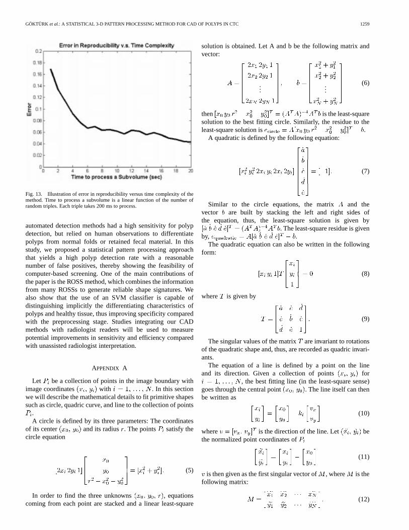
The current implementation of the algorithm takes on average20 s to process each candidate subvolume; We expect that opti-mized code could decrease the run time. Currently, 100 randomtriples are used to characterize a 3-D shape. A reduction in thenumber of random triples would reduce the time required; how-ever the trade off with accuracy needs to be explored. If a lessthan adequate number of views is used, the triples could be bi-ased toward some specific orientation in space. To find this ad-equate number, an easy attempt is to test the reproducibility ofthe ROSS method. That is, the shapes should have the same sig-natures regardless of the random views used in the analysis. Inorder to test the reproducibility, we conducted an experimentwith synthetic shapes, such as cylinders, ellipsoids and spheres.Two different random sets of orthogonal views are obtainedfrom each shape. The value ofis varied between five and 100.At the same time, the two signatures (and ) obtained by thetwo different random sets are compared by the following errorfunction:

(4)

where is the number of histogram bins. Ideally, the signaturesbelonging to the two random sets should be identical. Fig. 13illustrates the average error versus the time complexity. Here,we would like to remind that processing time for each randomtriple is approximately 200 ms, and the total processing time isa linear function of the number of planes used (). The figuredemonstrates that the number of random triples could be furtherreduced with only a negligible loss from the accuracy.

The algorithm is parallelizable, i.e., parallel processors couldprocess portions of the random planes independently, furtherreducing the required processing time. In the extreme case ofusing 100 parallel processors to process the 100 planes sepa-rately, the processing time reduces to 200 ms or less. Anotherway to parallelize is to divide the candidate volumes among theprocessors, i.e., one processor/candidate volume would result in20 s or less/patient.

V. CONCLUSION

Virtual colonoscopy is a promising new imaging techniqueto evaluate the human colon for precancerous polyps. Due tothe large amount of radiologist time involved in reviewing hun-dreds of images in a search for small lesions, CAD is necessaryto make the approach efficient and cost-effective. Previous


Fig. 13. Illustration of error in reproducibility versus time complexity of themethod. Time to process a subvolume is a linear function of the number ofrandom triples. Each triple takes 200 ms to process.

automated detection methods had a high sensitivity for polypdetection, but relied on human observations to differentiatepolyps from normal folds or retained fecal material. In thisstudy, we proposed a statistical pattern processing approachthat yields a high polyp detection rate with a reasonablenumber of false positives, thereby showing the feasibility ofcomputer-based screening. One of the main contributions ofthe paper is the ROSS method, which combines the informationfrom many ROSSs to generate reliable shape signatures. Wealso show that the use of an SVM classifier is capable ofdistinguishing implicitly the differentiating characteristics ofpolyps and healthy tissue, thus improving specificity comparedwith the preprocessing stage. Studies integrating our CADmethods with radiologist readers will be used to measurepotential improvements in sensitivity and efficiency comparedwith unassisted radiologist interpretation.

APPENDIX A

Let be a collection of points in the image boundary withimage coordinates with . In this sectionwe will describe the mathematical details to fit primitive shapessuch as circle, quadric curve, and line to the collection of points

.A circle is defined by its three parameters: The coordinates

of its center and its radius . The points satisfy thecircle equation

(5)

In order to find the three unknowns , equationscoming from each point are stacked and a linear least-square

solution is obtained. Let A and b be the following matrix andvector:

......

(6)

then is the least-squaresolution to the best fitting circle. Similarly, the residue to theleast-square solution is .

A quadratic is defined by the following equation:

(7)

Similar to the circle equations, the matrix and thevector are built by stacking the left and right sides ofthe equation, thus, the least-square solution is given by

. The least-square residue is givenby, .

The quadratic equation can also be written in the followingform:

(8)

where is given by

(9)

The singular values of the matrix are invariant to rotationsof the quadratic shape and, thus, are recorded as quadric invari-ants.

The equation of a line is defined by a point on the lineand its direction. Given a collection of points for

, the best fitting line (in the least-square sense)goes through the central point . The line itself can thenbe written as

(10)

where is the direction of the line. Let bethe normalized point coordinates of

(11)

is then given as the first singular vector of, where is thefollowing matrix:

(12)


Given and the best fitting line equation is complete.For any point , the error to this line is given as

(13)

REFERENCES

[1] P. J. Wingo, “Cancer statistics,”Ca Cancer J. Clin., vol. 45, pp. 8–30,1995.

[2] R. F. Thoeni and I. Laufer, “Polyps and cancer,” inTextbook of Gastroin-testinal Radiology. Philadelphia, PA: Saunders, 1994, p. 1160.

[3] S. J. Winawer, A. G. Zauber, M. N. Ho, M. J. O’Brien, L. S. Gottlieb,S. S. Sternberg, and J. D. Waye, “Prevention of colorectal cancer bycolonoscopy polypectomy,”N. Eng. J. Med., vol. 329, pp. 1977–1981,1993.

[4] D. M. Eddy, “Screening for colorectal cancer,”Ann. Intern. Med., vol.113, pp. 373–384, 1990.

[5] C. G. Coin, F. C. Wollett, J. T. Coin, M. Rowland, R. K. Deramos, and R.Dandrea, “Computerized radiology of the colon: A potential screeningtechnique,”Comput. Radiol., vol. 7, no. 4, pp. 215–221, 1983.

[6] A. S. Chaoui, M. A. Blake, M. A. Barish, and H. M. Fenlon, “Virtualcolonoscopy and colorectal cancer screening,”Abdom. Imag., vol. 25,no. 2, pp. 361–367, 2000.

[7] C. D. Johnson and A. H. Dachman, “CT colonography: The next colonscreening examination?,”Radiology, vol. 216, no. 2, pp. 331–341, 2000.

[8] D. J. Vining, “Virtual colonoscopy,”Gastrointest. Endosc. Clin. N.Amer., vol. 7, no. 2, pp. 285–291, 1997.

[9] A. K. Hara, C. D. Johnson, J. E. Reed, D. A. Ahlquist, H. Nelson, R.L. Ehman, C. H. McCollough, and D. M. Ilstrup, “Detection of col-orectal polyps by computed tomographic colography: Feasibility of anovel technique,”Gastroenterology, vol. 110, no. 1, pp. 284–290, 1996.

[10] M. Macari, A. Milano, M. Lavelle, P. Berman, and A. J. Megibow,“Comparison of time-efficient CT colonography with twoand three-di-mensional colonic evaluation for detecting colorectal polyps,”Amer. J.Roentgenol., vol. 174, no. 6, pp. 1543–1549, 2000.

[11] A. K. Hara, C. D. Johnson, J. E. Reed, D. A. Ahlquist, H. Nelson, R. L.MacCarty, W. S. Harmsen, and D. M. Ilstrup, “Detection of colorectalpolyps with CT colography: Initial assessment of sensitivity and speci-ficity,” Radiology, vol. 205, no. 1, pp. 59–65, 1997.

[12] D. K. Rex, D. Vining, and K. K. Kopecky, “An initial experience withscreening for colon polyps using spiral CT with and without CT colog-raphy,”Gastrointest. Endosc., vol. 50, no. 3, pp. 309–313, 1999.

[13] American Society for Gastrointestinal Endoscopy ASGE, “Technologystatus evaluation: Virtual colonoscopy: November 1997,”Gastrointest.Endosc., vol. 48, no. 6, pp. 708–710, 1998.

[14] A. H. Dachman, J. K. Kimiyoshi, C. M. Boyle, Y. Samara, K. R.Hoffmann, D. T. Rubin, and I. Hanan, “CT colonography with three-di-mensional problem solving for detection of colonic polyps,”Amer. J.Roentgenol., vol. 171, no. 4, pp. 989–995, 1998.

[15] C. F. Beaulieu, Jr., R. B. Jeffrey, C. Karadi, D. S. Paik, and S. Napel,“Display modes for CT colonography—Part II: Blinded comparison ofaxial CT and virtual endoscopic and panoramic endoscopic volume-ren-dered studies,”Radiology, vol. 212, no. 1, pp. 203–212, 1999.

[16] R. M. Summers, C. F. Beaulieu, L. M. Pusanik, J. D. Malley, R. B.Jeffrey, D. I. Glazer, and S. Napel, “Automated polyp detector forCT colonography: Feasibility study,”Radiology, vol. 216, no. 1, pp.284–290, 2000.

[17] H. Yoshida, Y. Masutani, P. M. MacEneaney, K. Doi, Y. Kim, and A. H.Dachman, “Detection of colonic polyps in CT colonography based ongeometric features,”Radiology, vol. 217, no. P, p. 582, 2000.

[18] S. B. Göktürk and C. Tomasi, “A graph method for the conservativedetection of polyps in the colon,” inProc. 2nd Int. Symp. VirtualColonoscopy, Boston, MA, 2000.

[19] D. S. Paik, C. F. Beaulieu, R. B. Jeffrey, J. Yee, A. M. Steinauer-Gebauer,and S Napel, “Computer aided detection of polyps in CT colonography:Free response roc evaluation of performance,”Radiology, vol. 217, no.SS, p. 370, 2000.

[20] D. S. Paik, C. F. Beaulieu, R. B. Jeffrey, C. Karadi, and S. Napel, “Detec-tion of polyps in CT colonography: A comparison of a computer aideddetection algorithm to 3-D visualization methods,” inRadiological So-ciety of North America 85th Scientific Sessions. Chicago, IL: Radio-logical Soc. N. Amer., 1999, p. 428.

[21] S. B. Göktürk, C. Tomasi, B. Acar, D. S. Paik, C. F. Beaulieu, andS. Napel, “A learning method for automated polyp detection,” inProc. Medical Image Computing and Computer-Assisted Intervention(MICCAI’01), Utrecht, The Netherlands, pp. 85–93.

[22] R. C. Gonzalez and R. E. Woods,Digital Image Processing. Reading,MA: Addison-Wesley, 1993.

[23] M. K. Hu, “Visual pattern recognition by moment invariants,”IRE Trans.Inform. Theory, vol. IT-8, pp. 179–187, 1962.

[24] R. M. Gray, Entropy and Information Theory. Berlin, Germany:Springer-Verlag, 1990.

[25] J. A. Hartigan and M. A. Wong, “A k-means clustering algorithm,”Appl.Statist., pp. 100–108, 1979.

[26] V. N. Vapnik, The Nature of Statistical Learning Theory. New York:Springer, 1995.

[27] B. Schölkopf,Support Vector Learning. Munich, Germany: R. Olden-bourg Verlag, 1997.

[28] K. Veropoulos, C. Campbell, and N. Cristianini, “Controlling the sensi-tivity of support vector machines,” presented at the Int. Joint Conf. AI(IJCAI’99), Stockholm, Sweden.

[29] C. Campbell. Kernel methods: A survey of current techniques. [Online].Available: http://citeseer.nj.nec.com/campbell00kernel.html.

Documents

A statistical 3-D pattern processing method for computer-aided detection of polyps in CT colonography