A State-Space Mixed Membership Blockmodel for Dynamic ...epxing/papers/2010/xing_fu_song_aoas09.pdf · A STATE-SPACE MIXED MEMBERSHIP BLOCKMODEL ... illustrated this model on the

Submitted to the Annals of Applied Statistics

arXiv: stat.ML/0901.0135

A STATE-SPACE MIXED MEMBERSHIP BLOCKMODEL

FOR DYNAMIC NETWORK TOMOGRAPHY

By Eric P. Xing ∗, Wenjie Fu, and Le Song

School of Computer Science, Carnegie Mellon University

In a dynamic social or biological environment, the interactionsbetween the actors can undergo large and systematic changes. Inthis paper, we propose a model-based approach to analyze what wewill refer to as the dynamic tomography of such time-evolving net-works. Our approach offers an intuitive but powerful tool to inferthe semantic underpinnings of each actor, such as its social rolesor biological functions, underlying the observed network topologies.Our model builds on earlier work on a mixed membership stochasticblockmodel for static networks, and the state-space model for track-ing object trajectory. It overcomes a major limitation of many currentnetwork inference techniques, which assume that each actor plays aunique and invariant role that accounts for all its interactions withother actors; instead, our method models the role of each actor as atime-evolving mixed membership vector that allows actors to behavedifferently over time and carry out different roles/functions when in-teracting with different peers, which is closer to reality. We presentan efficient algorithm for approximate inference and learning usingour model; and we applied our model to analyze a social networkbetween monks (i.e., the Sampson’s network), a dynamic email com-munication network between the Enron employees, and a rewiringgene interaction network of fruit fly collected during its full life cycle.In all cases, our model reveals interesting patterns of the dynamicroles of the actors.

1. Introduction. Networks are a fundamental form of representationof complex systems. In many problems arising in biology, social sciences andvarious other fields, it is often necessary to analyze populations of entitiessuch as molecules or individuals, also known as “actors” in some networkliterature, interconnected by a set of relationships such as regulatory inter-actions, friendships, and communications. Studying networks of these kindscan reveal a wide range of information, such as how molecules/individualsorganize themselves into groups; which molecules are the key regulator orwhich individuals are in positions of power; and how the patterns of biolog-ical regulations or social interactions are likely to evolve over time.

∗To whom corresponds should be addressed.Keywords and phrases: Dynamic Networks, Network Tomography, Mixed Membership

Stochastic Blockmodels, State Space Models

1

http://www.imstat.org/aoas/

http://arxiv.org/abs/stat.ML/0901.0135

2 XING, FU, AND SONG.

In this paper, we investigate an intriguing statistical inference problemof interpreting the dynamic behavior of temporally evolving networks basedon a concept known as network tomography. Borrowed from the vocabularyof magnetic resonance imaging, the term “network tomography” was firstintroduced by Vardi (1996) to refer to the study of a network’s internal char-acteristics using information derived from the observed network. In mostreal-world complex systems such as a social network or a gene regulationnetwork, the measurable attributes and relationships of vertices (or nodes)in a network are often functions of latent temporal processes of events whichcan fluctuate, evolve, emerge and terminate stochastically. Here we definenetwork tomography more specifically as the latent semantic underpinningsof entities in both static and dynamic networks. For example, it can standfor the latent class labels, social roles, or biological functions undertaken bythe nodal entities, or the measures on the affinity, compatibility, and coop-erativity between nodal states that determine the edge probability. Our goalis to develop a statistical model and algorithms with which such informationcan be inferred from dynamically evolving networks via posterior inference.

We will concern ourselves with three specific real world time-evolvingnetworks in our empirical analysis: 1) the well-known Sampson’s undirectedsocial networks (Sampson, 1969) of 18 monks over 3 time episodes, whichare recorded during an interesting timeframe that preludes a major conflictfollowed by a mass departure of the monks, and therefore an interestingexample case to infer nodal causes behind dramatic social changes; 2) thetime series of email-communication networks of ENRON employees beforeand during the collapse of the company, which may have recorded interest-ing and perhaps sociologically illuminating behavioral patterns and trendsunder various business operation conditions; and 3) the sequence of geneinteraction networks estimated at 22 time points during the life span ofDrosophila melanogaster, a fruit fly commonly used as a lab model to studythe mechanisms of animal embryo development, which captures transientregulatory events as the animal aging.

Inference of network tomography is fundamental for understanding theorganization and function of complex relational structures in natural, socio-cultural, and technological systems such as the ones mentioned above. In asocial system such as a company employee network, network tomography cancapture the latent social roles of individuals; inferring such roles based onthe social interactions among individuals is fundamental for understandingthe importance of members in a network, for interpreting the social struc-ture of various communities in a network, and for modeling the behavioral,sociological, and even epidemiological processes mediated by the vertices in

DYNAMIC NETWORK TOMOGRAPHY 3

a network. In systems biology, network tomography often translates to latentbiochemical or genetic functions of interacting molecules such as proteins,mRNAs, or metabolites in a regulatory circuity; elucidating such functionsbased on the topology of molecular networks can advance our understandingof the mechanisms of how a complex biological system regulates itself andreacts to stimuli. More broadly, network tomography can lead to importantinsights to the robustness of network structures and their vulnerabilities;the cause and consequence of information diffusion; and the mechanism ofhierarchy and organization formation. By appropriately modeling networktomography, a network analyzer can also simulate and reason about the gen-erative mechanisms of networks, and discover changing roles among actorsin networks, which will be relevant for activity and anomaly detection.

There has been a variety of successes in network analysis based on var-ious formalisms. For example, researchers have found trends in a wide va-riety of large-scale networks, including scale-free and small-world proper-ties (Barabasi and Albert, 1999; Kleinberg, 2000). Other successes includethe formal characterization of otherwise intuitive notions, such as “group-ness” which can be formally characterized in the networks perspective usingmeasures of structural cohesiveness and embeddedness (Moody and White,2003), detecting outbreaks (Leskovec et al., 2007), and characterizing macro-scopic properties of various large social and information networks (Leskovec et al.,2008). Additionally, there has been progress in statistical modeling of socialnetworks, traditionally focusing on descriptive models such as the expo-nential random graph models, and more recently moving toward variouslatent space models that estimate an embedding of the network in a la-tent semantic space, as we review shortly in Section 2. A major limitationof most current methods for network modeling and inference (Hoff et al.,2002; Li and McCallum, 2006; Handcock et al., 2007) is that, they assumeeach actor, such as a social individual or a biological molecule in a network,undertakes a single and invariant role (or functionality, class label, etc., de-pending on the domain of interest), when interacting with other actors. Inmany realistic social and biological scenarios, every actor can play multipleroles (or under multiple influences) and the specific role being played depen-dents on whom the actor is interacting with; and the roles undertaken by anactor can change over time. For example, during a developmental process oran immune response in a biological system, there may exist multiple under-lying “themes” that determine the functionalities of each molecule and theirrelationships to each other, and such themes are dynamical and stochastic.As a result, the molecular networks at each time point are context-dependentand can undergo systematic rewiring, rather than being i.i.d. samples from a


single underlying distribution, as assumed in most current biological networkstudies. We are interested in understanding the mechanisms that drive thetemporal rewiring of biological networks during various cellular and physio-logical processes, and similar phenomena in time-varying social networks.

In this paper, we propose a new Bayesian approach for network tomo-graphic inference that will capture the multi-facet, context-specific, andtemporal nature of an actor’s role in large, heterogeneous, and evolvingdynamic networks. The proposed method will build on a modified version ofthe mixed membership stochastic blockmodel (MMSB) (Airoldi et al., 2008),which enables network links to be realized by role-specific local connectionmechanisms; each link is underlined by a separately chosen latent functionalcause, and each vertex can have fractional involvement in multiple functionsor roles which are captured by a mixed membership vector. Thereby the pro-posed model supports analyzing patterns of interactions between actors viastatistically inferring an “embedding” of a network in a latent “tomographic-space” via the mixed membership vectors. For example, the characteristics ofgroup profiles of actors revealed by the mixed membership vectors can offerimportant and intuitive community structures in the networks in question.

Modeling embedding of networks in latent state space offers an intu-itive but powerful approach to infer the semantic underpinnings of eachactor, such as its biological or social roles or other entity functions, un-derlying the observed network topologies. Via such a model, one can mapevery actor in a network to a position in a low-dimensional simplex, wherethe roles/functions of the actors are reflected in the role- or functional-coordinates of the actors in the latent space and the relationships amongactors are reflected in their Euclidian distances. We can naturally capturethe dynamics of role evolution of actors in such a tomographic-space, andother latent dynamic processes driving the network evolution by furthermoreapplying a state-space model (SSM) popular in object tracking over the po-sitions of the tomographic-embeddings of all actors, where a logistic-normal

mixed membership stochastic blockmodel is employed as the emission modelto define time-specific condition likelihood of the observed networks overtime. The resulting model shall be formally known as a state space mixed

membership stochastic blockmodel, but for simplicity in this paper we willrefer to it as a dynamic MMSB (or in short, dMMSB); and we will showthat this model allows one to infer the trajectory of the roles of each actorbased on the posterior distribution of its role-vector.

Given network data, the dMMSB can be learned based on maximum like-lihood principle using a variational EM algorithm (Ghahramani and Beal,2001; Xing et al., 2003; Ahmed and Xing, 2007), the resulting network pa-


rameters reveal not only mixed membership information of each actor overtime, but also other interesting regularities in the network topology. We willillustrated this model on the well-known Sampson’s monk social network,and then apply it to the time series of email network from Enron, and thesequence of time-varying genetic interaction networks estimated from theDrosophila genome-wise microarray time series, and we will present somepreviously unnoticed dynamic behaviors of network actors in these data.

The remaining part of the paper is organized as follows. In Section 2, webriefly review some related work. In Section 3 we present the dMMSB modelin detail. A Laplace variational EM algorithm for approximate inferenceunder dMMSB will be described in Section 4. In Section 5 we present casestudies on the monks network, the Enron network, and the Drosophila genenetwork using dMMSB, along with some simulation based validation of themodel. Some discussions will be given in Section 6. Algebraic details of thederivations of the inference algorithm are provided in the appendix.

2. Related work. There is a vast and growing body of literature onmodel-based statistical analysis of network data, traditionally focusing ondescriptive models such as the exponential random graph models (ERGMs)(Frank and Strauss, 1986; Wasserman and Pattison, 1996), and more re-cently moving toward more generative types of models such as those thatmodel the network structure as being caused by the actors’ positions in alatent “social space” (Hoff et al., 2002). Among these models, some variantsof the ERGMs, such as the stochastic block models (Holland et al., 1983;Fienberg et al., 1985; Wasserman and Pattison, 1996; Snijders, 2002), clus-ter network vertices based on their structural equivalency (Lorrain and White,1971). The latent space models (LSM) instead project nodes onto a latentspace, where their similarities can be visualized and explored (Hoff et al.,2002; Hoff, 2003; Handcock et al., 2007). The mixed membership stochas-tic blcokmodel proposed in Airoldi et al. (2005, 2008) integrates ideas fromthese models, but went further by allowing each node to belong to multi-ple blocks (i.e., groups) with fractional membership. Variants of the mixedmembership model have appeared in population genetics (Pritchard et al.,2000), text modeling (Blei et al., 2003a), analysis of multiple disability mea-sures (Erosheva and Fienberg, 2005), etc. In most of these cases, mixedmembership models are used as a latent-space projection method to projecthigh-dimensional attribute data into a lower-dimensional “aspect-space”, asa normalized mixed membership vector, which reflects the weight of eachlatent aspect (e.g., roles, functions, topics, etc.) associated with an ob-ject (Erosheva et al., 2004). The mixed membership vectors often serve as


a surrogate of the original data for subsequent analysis such as classifi-cation (Blei et al., 2003b). The MMSB model developed earlier has beenapplied for role identification in Sampson’s 18-monk social network and func-tional prediction in a protein-protein interaction network (PPI) (Airoldi et al.,2005, 2008). It uses the aforementioned mixed membership vector to definean actor-specific multinomial distribution, from which specific actor rolescan be sampled when interacting with other actors. For each monk, it yieldsa multi-class social-identity prediction which captures the fact that his in-teractions with different other monks may be under different social contexts.For each protein, it yield a multi-class functional prediction which capturesthe fact that its interactions with different proteins may be under differentfunctional contexts.

We intend to use the state space model (SSM) popular in object trackingand trajectory modeling for inferring underlying functional changes in net-work entities, and sensing emergence and termination of “function themes”underlying network sequences. This scheme has been adopted in a num-ber of recent work on extracting evolving topical themes in text docu-ments (Blei and Lafferty, 2006b; Wang and McCallum, 2006) or author em-beddings (Sarkar and Moore, 2005) based on author, text, and referencenetwork of archived publications.

3. Modeling Dynamic Network Tomography. Consider a tempo-ral series of networks {G(1), . . . , G(T )} over a vertex set V , where G(t) ≡{V,E(t)} represents the network observed at time t. In this paper, we as-sume that N = |V | is invariant over time; thus E(t) ≡ {e(t)

i,j}Ni,j=1 denote the

set of (possibly transient) links at time t between a fixed set of N vertices.To model both the multi-class nature of every vertex in a network, and

the latent semantic characteristics of the vertex-classes and their relation-ships to inter-vertices interactions, we assume that at any time point, everyvertex vi ∈ V in the network, such as a social actor or a biological molecule,can undertake multiple roles or functions realized from a predefined latenttomographic space according to a time-varying distribution Pt(·); and theweights (i.e., proportion of “contribution”) of the involved roles/functionscan be represented by a normalized vector ~π(t)

i of fixed dimension K. We referto each role, function, or other domain-specific semantics underlying the ver-tices as a membership of a latent class. Earlier stochastic blockmodel of net-works restricted each vertex to belong to a single and invariant membership.In this paper, we assume that each vertex can have mixed memberships, thatis, it can undertake multiple roles/functions within a single network wheninteracting with various network neighbors with different roles/functions,


and the vector of proportions of the mixed-memberships, ~π(t)

i , can evolveover time. Furthermore, we assume that the links between vertices are in-stantiated stochastically according to a compatibility function over the rolesundertaken by the vertex-pair in question, and we define the compatibil-ity coefficients between all possible pair of roles using a time-evolving role-compatibility matrix B(t) ≡ {β(t)

k,l}.

3.1. Static Mixed Membership Stochastic Blockmodel. Under a basic MMSBmodel, as first proposed in Airoldi et al. (2005), network links can be real-ized by a role-specific local interaction mechanisms: the link between eachpair of actors, say (i, j), is instantiated according to the latent role specifi-cally undertaken by actor i when it is to interact with j, and also the latentrole of j when it is to interact with i. More specifically, suppose that eachdifferent role-pair, say roles k and l, between actors has a unique probabil-ity distribution P (·|βk,l) of having a link between actor pairs with that rolecombination, then a basic mixed membership stochastic blockmodel positsthe following generative scheme for a static network:

1. For each vertex i, draw the mixed-membership vector: ~πi ∼ P (·|θ)

2. For each possible interacting vertex j of vertex i, draw the link indicator ei,j ∈ {0, 1}as follows:

• draw latent roles ~zi→j ∼ Multinomial(·|~πi, 1), ~zj←i ∼ Multinomial(·|~πj , 1),where ~zi→j denotes the role of actor i when it is to interact with j, and ~zj←i

denotes the role of actor j when it is approached by i. Here ~zi→j and ~zj←i

are unit indictor vectors in which one element is one and the rest are zero; itrepresents the k-th role if and only if the k-th element of the vector is one,for example, zi→j,k = 1 or zj←i,k = 1.

• and draw ei,j | (zi→j,k = 1, zj←i,l = 1) ∼ Bernoulli(·|βk,l).

Specifically, the generative model above defines a conditional probabilitydistribution of the relations E = {ei,j} among vertices in a way that re-flects naturally interpretable latent semantics (e.g., roles, functions, clusteridentities) of the vertices. The link ei,j represents a binary actor-to-actorrelationship. For example, the existence of a link could mean that a packagehas been sent from one person to another, or one has a positive impressionon another, or one gene is regulated by another. Each vertex vi is associatedwith a set of latent membership labels {~zi→·, ~zi←·} (if the links are undi-rected, as in a PPI, then we can ignore the asymmetry of ”→” and ”←”).Thus the semantic underpinning of each interaction between vertices is cap-tured by a pair of instantiated memberships unique to this interaction; andthe nature and strength of the interaction is controlled by the compatibilityfunction determined by this pair of memberships instantiation. For example,if actors A and C are of role X while actors B and D are of role Y , we may


expect that the relationship from A to B is likely to be the same as relation-ship from C to D, because both of them are from a role-X actor to a role-Yactor. In this sense, a role is like a class label in a classification task. How-ever, under an MMSB model, an actor can have different role instantiationswhen interacting with different neighbors in the same network.

The role-compatibility matrix B ≡ {βk,l} decides the affinity betweenroles. In some cases, the diagonal elements of the matrix may dominateover other elements, which means actors of the same role are more likelyto connect to each other. In the case where we need to model differentialpreference among different roles, richer block patterns can be encoded in therole-compatibility matrix. The flexibility of the choices of the B matrix giverise to strong expressivity of the model to deal with complex relational pat-terns. If necessary, a prior distribution over elements in B can be introduced,which can offer desirable smoothing or regularization effects.

Crucial to our goal of role-prediction and role-evolution modeling for net-work data, is the so called mixed membership vector ~πi, also referred toas “role vector”, of the mixed-membership coefficients in the above gener-ative model, which represents the overall role spectrum of each actor andsuccinctly captures the probabilities of an actor involving in different roleswhen this actor interacts with another actor. Much of the expressiveness ofthe mixed-membership models lies in the choice of the prior distribution forthe mixed-membership coefficients ~πi, and the prior for the interaction coef-ficients {βk,l}. For example, in Airoldi et al. (2005, 2008), a simple Dirichletprior was employed because it is conjugate to the multinomial distributionover every latent membership label {~zi→·, ~zi←·} defined by the relevant ~πi.In this paper, to capture non-trivial correlations among the weights (i.e., theindividual elements within ~πi) of all latent roles of a vertex, and to allow oneto introduce dynamics to the roles of each actor when modeling temporalprocesses such as a cell cycle, we employ a logistic-normal distribution overa simplex (Aitchison and Shen, 1980; Aitchison, 1986; Ahmed and Xing,2007). The resulting model is referred to as a logistic-normal MMSB, orsimply LNMMSB.

Under a logistic normal prior, assuming a centered logistic transforma-tion, the first sampling step for ~πi ≡ [πi,1, . . . , πi,K ] in the canonical mixedmembership generative model above can be broken down into two sub-steps:first draw ~γi according to:

(1) ~γi ∼ Normal(~µ,Σ);


then map it to the simplex via the following logistic transformation:

πi,k = exp{γi,k − C(~γi)}, ∀k = 1, . . . ,K(2)

where C(~γi) = log(

K∑

k=1

exp{γi,k})

.(3)

Here C(~γi) is a normalization constant (i.e., the log partition function).Due to the normalizability constrain of the multinomial parameters, ~πi onlyhas K − 1 degree of freedom. Thus we only need to draw the first K − 1components of ~γi from a (K − 1)-dimensional multivariate Gaussian, andleave γi,K = 0. For simplicity, we omit this technicality in the forth cominggeneral description and operation of our model.

Under a dynamic network tomography model, the prior distributions ofrole weights of every vertex Pt(·), and the role-compatibility matrix B,can both evolve over time. Conditioning on the observed network sequence{G(1), . . . , G(T )}, our goal is to infer the trajectories of role vectors ~π(t)

i in thelatent social space or biological function space. In the following, we presenta generative model built on elements from the classical state-space modelfor linear dynamic systems and the static logistic normal MMSB describedabove for random graphs for this purpose.

3.2. Dynamic Logistic-Normal Mixed Membership Stochastic Blockmodel.

We propose to capture the dynamics of network evolution at the level ofboth the prior distributions of the mixed membership vectors of vertices, andthe compatibility functions governing role-to-role relationships. In this waywe capture the dynamic behavior of the generative system of both verticesand relations. Our basic model structure is based on the well-known state-space model, which defines a linear dynamic transformation of the mixedmembership priors over adjacent time points:

(4) ~µ(t) = A~µ(t−1) + ~w(t), for t ≥ 1

where ~µ(t) represents the mean parameter of the prior distribution of thetransformed mixed membership vectors of all vertices at time t, and ~w(t) ∼N (0,Φ) represents normal transition noise for the mixed membership prior,and the transition matrix A shapes the trajectory of temporal transfor-mation the prior. The LNMMSB model defined above now functions as anemission model within the SSM that defines the conditional likelihood ofthe network at each time point. Note that the linear system on ~µ(t) can leadto a bursty dynamics for latent admixing vector π(t)

i through the LNMMSBemission model. Starting from this basic structure, we propose to develop


a dynamical model for tracking underlying functional changes in networkentities and sensing emergence and termination of “function themes”.

Given a sequence of network topologies over the same set of nodes, here isan outline of the generative process under such a model (a graphical modelrepresentation of this model is illustrated in Figure 1):

• State-Space Model for Mixed Membership Prior:

– ~µ(1) ∼ Normal(ν,Φ),sample the mean of the mixed membershipprior at time 1.

For t = 1, . . . , T :

– ~µ(t) = Normal(A~µ(t−1),Φ),sample the means of the mixed member-ship priors over time.

• State-Space Model for Role-Compatibility Matrix:

For k = 1, . . . ,K and k′ = 1, . . . ,K,

– η(1)

k,k′∼ Normal(ι, ψ),

sample the compatibility coefficient be-tween role k and k′ at time 1.

For t = 1, . . . , T :

– η(t)

k,k′∼ Normal(bη(t−1)

k,k′, ψ),

sample compatibility coefficients over sub-sequent time points.

– β(t)

k,k′=

exp(η(t)

k,k′)

exp(η(t)

k,k′)+1

,compute compatibility probabilities via lo-gistic transformation.

• Logistic-Normal Mixture Membership Model for Networks

For each node n = 1, . . . , N , at each time point t = 1, . . . , T :

– ~π(t)

i ∼ LogisticNormal(

~µ(t),Σ(t)) sample a k dimensional mixed mem-

bership vector;

For each pair of nodes (i, j) ∈ [1, N ] × [1, N ]:

– ~z(t)

i→j ∼ Multinomial(

~π(t)

i , 1) sample membership indicator for

the donor

– ~z(t)

j←i ∼ Multinomial(

~π(t)

j , 1) sample membership indicator for

the acceptor

– e(t)

i,j ∼ Bernoulli(

~z(t) ′

i→j B(t)~z

(t)j←i

)

sample the links between nodes.

Specifically, we assume that the mixed membership vector ~π for each actorfollows a time-specific logistic normal prior LN (~µ(t),Σ(t)), whose mean ~µ(t)

is evolving over time according to a linear Gaussian model. For simplicity,we assume that the Σ(t) which captures time-specific topic correlations isindependent across time.

It is noteworthy that unlike a standard SSM of which the latent statewould emit a single output (i.e., an observation or a measurement) at eachtime point, the dMMSB model outlined above generates N emissions each


Fig 1. A graphical model representation of the dynamic logistic-normal mixed membershipstochastic blockmodel. The part enclosed by the dotted lines is a logistic-normal MMSB.

time, one corresponding to the (pre-transformed) mixed-membership vector~γ(t)

i of each vertex. To directly apply the Kalman filter and Rauch-Tung-Striebel smoother for posterior inference and parameter estimation underdMMSB, we introduce an intermediate random variable ~Y (t) = 1

N

∑

i ~γ(t)

i ; it

is easy to see that ~Y (t) follows a standard SSM re-parameterized from theoriginal dMMSB:

~Y (t) ∼ Normal(

~µ(t),Σ(t)

N

)

, t = 1, . . . , T.(5)

In principle, we can use the above membership evolution model to capturenot only membership correlation within and between vertices at a specifictime (as did in Blei and Lafferty (2006a)), but also dynamic coupling (i.e.,co-evolution) of membership proportions via covariance matrix Φ. In thesimplest scenario, when A = I and Φ = σI, this model reduces to randomwalk in the membership-mixing space. Since in most realistic temporal seriesof networks, both the role-compatibility functions between vertices, and thesemantic representations of membership-mixing are unlikely to be invariantover time, we expect that even a random walk mixed-membership evolutionmodel can provide a better fit of the data than a static model that ignoresthe time stamps of all networks.


4. Variational Inference. Due to difficulties in marginalization overthe super-exponential state space of latent variables ~z and ~π, even the ba-sic MMSB model based on a Dirichlet prior over the role vectors ~π is in-tractable (Airoldi et al., 2005, 2008). With the additional difficulty in in-tegration of ~π under a logistic normal prior where a closed-form solutionis unavailable, exact posterior inference of the latent variables of interest,and direct EM estimation of the model parameters is infeasible. In this sec-tion, we present a Laplace variational approximation scheme based on thegeneralized means field (GMF) theorem (Xing et al., 2003) to infer the la-tent variables and estimate the model parameters. This scheme requiresone additional approximating step on top of the variational approxima-tion developed in (Airoldi et al., 2008), but we will show empirically inSection 5.1.1 that this step does not introduce much additional error. TheGMF approach is modular, that is, we can approximate the joint posterior

p(

{~z(t), ~π(t), ~µ(t), B(t)}Tt=1|Θ, {G(t)}T

t=1

)

where Θ denotes the model parame-

ters, by a factored approximate distribution:

(6) q(

{~z(t), ~π(t), ~µ(t), B(t)}T

t=1

)

= q1

(

{~z(t), ~π(t)}T

t=1

)

q2

(

{~µ(t)}T

t=1

)

q3

(

{B(t)}T

t=1

)

,

where q1() can be shown to be the marginal distribution of {~z(t), ~π(t)}Tt=1 un-

der a reparameterized LNMMSB, and q2() and q3() are SSMs over {~µ(t)}Tt=1

and {B(t)}Tt=1, respectively, with emissions related to expectation of {~z(t), ~π(t)}T

t=1

under q1(). This can be shown by minimizing the Kulback Leibler divergencebetween q() and p() over arbitrary choices of q1(), q2() and q3(), as provenin (Xing et al., 2003). The computation of the variational parameters of eachof these approximate marginals leads to a coupling of all the marginals, asapparent in the descriptions in the subsequent subsections. But once thevariational parameters are solved, inference on any latent variable of inter-est under the joint distribution p(), which is intractable, can be approxi-mated by a much simpler inference on the same variable in one of the qi()marginals that contains the variables of interest. Bellow we briefly outlinesolutions to each of these marginals of subset of variables, which exactlycorrespond to the three building blocks of the dMMSB model outlined inSection 3.2. (Since µ(t) and B(t) both follow a standard SSM, for simplicity,we only show the solution to q2() over µ(t), and treat B(t) as an unknowninvariant constant to be estimated.)

4.1. Variational approximation to logistic-normal MMSB. For a staticMMSB, the inference problem is to estimate the role-vectors given modelparameters and observations. That is, model parameters ~µ, Σ and B areassumed to be known besides the observed variables E, and we want to


compute estimates of the role vectors ~γ· along with role indicators ~z·→· and~z·←·. (Under dMMSB, ~µ is in fact unknown, but we will discuss shortly howto estimate it outside of the MMSB inference detailed bellow.)

Under the LNMMSB, ignoring time and vertex indices, the marginal pos-terior of latent variables ~γ (the pre-transformed ~π) and ~z is:

p(~γ·, ~z·→·, ~z·←· | ~µ,Σ, B,E) ∝∏

i

p(~γi | ~µ,Σ)×(7)

∏

i,j

p(~zi→j , ~zj←i | ~γi, ~γj)p(eij | ~zi→j, ~zj←i, B)

Marginalization over all but one hidden variables to predict, say ~γi, isintractable under the above model. Based on the GMF theory, we ap-proximate p(~γ·, ~z·→·, ~z·←· | ~µ,Σ, B,E) with a product of simpler marginalsq() = qγ()qz(), each on a cluster of latent variable subset, i.e., {~γi} and{~zi→j , ~zj←i}. Xing et al. (2003) proved that under GMF approximation, theoptimal solution, q(), of each marginal over the cluster of variables is iso-morphic to the true conditional distribution of the cluster given its expected

Markov Blanket. That is,

qγ(~γi) = p(~γi | ~µ,Σ, 〈~zi→·〉qz , 〈~zi←·〉qz)(8)

qz(~zi→j , ~zj←i) = p(~zi→j , ~zj←i | eij , B, 〈~γi〉qγ , 〈~γj〉qγ )(9)

These equations define a fixed point for qγ and qz. The optimal marginaldistribution of the variables in one cluster is updated when we fix themarginal of all the other variables, in turn. The update continues until thechange is neglectable.

The update formula for cluster marginal of (~zi→j , ~zj←i) is straightforward.It follows a multinomial distribution with K ×K possible outcomes 1 :

qz(~zi→j, ~zj←i) ∝ p(~zi→j | 〈~γi〉qγ ) p(~zj←i | 〈~γj〉qγ ) p(eij | ~zi→j , ~zj←i, B)(10)

∼ Multinomial(~δij)

where δij(u,v) ≡1C

exp(〈γi,u〉qγ + 〈γj,v〉qγ ) βeiju,v (1 − βu,v)

1−eij , and C is thenormalization function to keep

∑

(u,v) δij(u,v) = 1. Furthermore, the expec-tation of z’s according to the multinomial distribution are

〈zi→j,u〉qz=

∑

v δij(u,v)∑

u,v δij(u,v)=∑

v

δij(u,v), 〈zj←i,v〉qz=

∑

u δij(u,v)∑

u,v δij(u,v)=∑

u

δij(u,v).

(11)

1The K ×K components are flatted into a one-dimension vector.


The update formula for ~γi can be derived similarly but some further ap-proximation is applied. First,

qγ(~γi) ∝ p(~γi | ~µ,Σ) p(〈~zi→·〉qz , 〈~zi←·〉qz | ~γi)(12)

= N (~γi; ~µ,Σ) exp(〈~mi〉qz

T ~γi − (2N − 2) C(~γi))

where mik =∑

j 6=i(zi→j,k + zi←j,k), 〈mik〉qz =∑N

j 6=i(〈zi→j,k〉qz + 〈zi←j,k〉qz),

and C(~γi) = log(∑K

k=1 exp{γi,k}). The presence of the normalization con-stant C(~γi) makes qγ un-integrable in closed-form. Therefore we apply aLaplace approximation to C(~γi) based on a second-order Taylor expansionaround γi (Ahmed and Xing, 2007), such that qγ(~γi) becomes a reparam-eterized multivariate normal distribution N (γi, Σi) (see Appendix A.1 fordetails). In order to get a good approximation, the point of expansion, γi,should be set as close to the query point as possible. Therefore, we set itto be the γi obtained from the previous iteration, i.e. γr+1

i = γri where r

denotes the iteration number.The inference algorithm iterates between Eq. 10 and Eq. 12 until conver-

gence when the relative change of log-likelihood is less than 10−6 in absolutevalue. The procedure is repeated multiple times with random initializationfor γi. The result having the best likelihood is picked as the solution.

4.2. Parameter Estimation for Logistic-Normal MMSB. The model pa-rameters ~µ, Σ and B have to be estimated from data E ≡ {eij}. In thesimplest case, where time evolution of ~µ and B is ignored, these can be donevia a straightforward EM-style procedure.

In the E step, we use the inference algorithm from Section 4.1 to com-pute the posterior distribution and expectation the latent variables by fix-ing the current parameters. In the M step, we re-estimate the parame-ters by maximizing the log-likelihood of the data using the posteriors ob-tained from the E-step. Under a LNMMSB, exact computation of the log-likelihood is intractable, hence we use an approximation method known asvariational EM. We obtain the following update formulas for variationalEM (Ghahramani and Beal, 2001): (See Appendix A.2 for an illustration ofthe derivation of the update for B.)

βk,l =

∑

i,j eijδij(k,l)∑

i,j δij(k,l), µ =

1

N

∑

i

γi, Σ =1

N

∑

i

Σi + Cov(γ1:N )(13)

The procedure for the learning can be summarized below:


Learning for Logistic-Normal MMSB:1. initialize B ∼ U [0, 1], ~µ ∼ N (0, I), Σ = 10I2. while not converged (Outer Loop)

2.1. Initialize q(~γi)2.2. while not converged and #iteration ≤ threshold (Inner Loop)

2.2.1. update q(~zi→j , ~zj←i) ∼ Multinomial(~δij)

2.2.2. update q(~γi) ∼ N (γi, Σi)2.2.3. update B

2.3. update ~µ, Σ

The convergence criterion is the same as in inference. It is worth notingthat the update of role-compatibility matrix B is in the inner loop, whichmeans that it is updated as frequently as mixed membership vectors ~γi. Thismakes sense because the role-compatibility matrix and mixed membershipvectors are closely coupled.

4.3. Variational approximation to dMMSB. When ~µ is time-evolving asin dMMSB, two aspects in the algorithms described in Sections 4.1 and 4.2need to be treated differently. First, unlike in Eq. (13), estimation of ~µ(t)

now must be done under an SSM, with {γ(t)

i } as the emissions at everytime point. Second, according to the GMF theorem, the µ appeared in allequations in Section 4.1 must now be replaced by the posterior mean of ~µ(t)

under this SSM. Bellow we first summarize the algorithm for dMMSB, fol-lowed by details of the update steps based on the Kalman Filter (KF) andthe Rauch-Tung-Striebel (RTS) smoother algorithms.

Inference for dMMSB:1. initialize all ~µ(t)

2. while not converged2.1. for each t

2.1.1. call the inference algorithm for MMSB on network E(t) in §4.1(by passing to it all current estimate of ~µ(t)),

and return the GMF approximation γ(t)i , Σ

(t)i

2.1.2. update the observations, ~Y (t) =∑

i γ(t)i /N

2.2. RTS smoother update ~µ(t) = µt|T based on {~Y (t)}T

t=1

Given all model parameters and all the emissions (the current estimate ofthe mixed membership vectors {γ(t)

i } of all vertices returned by the logisticnormal MMSB at each time point), posterior inference of the hidden states~µ(t) can be solved according to the following KF and RTS procedure. The


major update steps in the Kalman Filter are:

µt+1|t = Aµt|t = µt|t

Pt+1|t = APt|tAT + Φ = Pt|t + Φ

Kt+1 = Pt+1|t(Pt+1|t + Σt+1/N)−1

µt+1|t+1 = µt+1|t + Kt+1(~Yt+1 − µt+1|t)(14)

Pt+1|t+1 = Pt+1|t −Kt+1Pt+1|t(15)

where µt|s ≡ E (~µ(t) | ~Y1, . . . , ~Ys) and Pt|s ≡ Var(µ(t) | Y1, . . . , Ys). And themajor update steps in the Rauch-Tung-Striebel smoother are:

Lt = Pt|tAT P−1

t+1|t = Pt|tP−1t+1|t

µt|T = µt|t + Lt(µt+1|T − µt+1|t)(16)

Pt|T = Pt|t + Lt(Pt+1|T − Pt+1|t)LTt(17)

4.4. Parameter Estimation for dMMSB. We again use the variationalEM algorithm. The E-step uses the dMMSB inference algorithm in Sec-tion 4.3 for compute sufficient statistics µt|T ,∀t, and the logistic normalMMSB inference algorithm in Section 4.2 for computing all sufficient statis-

tics δ(t)ij(k,l). In the M-step, model parameters are updated by maximizing

the log-likelihood obtained from the E-step. From this on, we simplify thelinear transition model posed on matrix B and assume that it is constant.We derive the following updates for the model parameters B, ν,Φ,Σ(t) (SeeAppendix A.3 for some details):

βk,l =

∑

t

∑

i,j e(t)ij δ

(t)ij(k,l)

∑

t

∑

i,j δ(t)ij,(k,l)

(18)

Φ =1

T − 1

(

T−1∑

t=1

(µt+1|T − µt|T )(µt+1|T − µt|T )T +T−1∑

t=1

LtPt+1|T LTt

)

(19)

Σ(t) =1

N

(

∑

i

(µt|T − γ(t)i )(µt|T − γ

(t)i )T +

∑

i

Σ(t)i

)

(20)

ν = µ1|T(21)

The algorithm can be summarized below:


Learning for dMMSB:1. initialize B ∼ U [0, 1], ν ∼ N (0, I), ~µ(t) = ν, Φ = 10I, Σ(t) = 10I2. while not converged

2.1. Initialize all q(~γ(t)i )

2.2. while not converged2.2.1. foreach t

2.2.1.1. update q(~zi→j , ~zj←i) ∼ Multinomial(~δij)

2.2.1.2. update q(~γi) ∼ N (γi, Σi)2.1.2. update B

2.3. RTS smoother update, ~µ(t) = µt|T based on {~Y (t)}T

t=1

2.4. update ν, Φ, Σ(t)

Notice that in the above algorithm, the variational cluster marginalsq(~zi→j , ~zj←i), q(~γi), and q(~µ(1), . . . , ~µ(T )) each dependents on variational pa-rameters defined by other cluster marginals. Thus overall the algorithm isessentially a fixed-point iteration that will converge to a local optimum. Weuse multiple random restarts to obtain a near global optimum.

5. Experiments. In this section we validate the inference algorithmspresented in Section 4 on synthetic networks and demonstrate the advan-tages of the dMMSB model on the well-known Sampson’s monk network.Then we apply dMMSB to two large-scale real world datasets.

5.1. Synthetic networks. We first evaluate the logistic normal MMSB de-scribed in Section 3.1 in comparison with the earlier Dirichlet MMSB pro-posed by Airoldi et al. (2008), and then with the dMMSB model describedin Section 3.2. We investigate their differences in three major aspects: (i) Isthe Laplace variational inference algorithm adequate for accurately estimatethe mixed membership vectors? (ii) For a static network, does LNMMSBprovides a better fit to the data when different roles are correlated? And(iii) for dynamic networks, does dMMSB provides a better fit to the data?

5.1.1. Inference accuracy. We generated three sets of synthetic networkseach of which has 100 individuals and 3 roles, using 3 different sets role-vector priors and role-compatibility matrices, to mimic different real-lifesituations. Figure 2 shows the estimation errors with LNMMSB under thethree senarios. The results from the Dirichlet MMSB is very close to that ofLNMMSB and therefore not shown here.

For synthetic network I, most actors have a single role and the role-compatibility matrix is diagonal which means that actors connect mostly


I. 1

2

3 II. 1

2

3 III.1

2

3

true est. true est. true est.1 0 00 1 00 0 1

1 0 00 1 00 0 1

1 0.3 00.3 1 00.0 0 1

1 0.34 00.25 1 00 0 1

0.45 0 0.050 0.50 00 0 0.40

0.52 0 00 0.52 00 0 0.39

Fig 2. Results of inference and learning with LNMMSB on representative synthetic net-works from scenario I to III. In the top row, the figure in each cell displays the estimatedrole-vectors. They are projected onto a simplex along with the ground truth: a circle rep-resents the position of a ground truth; a cross represents an estimated position; and, eachtruth-estimation pair is linked by a grey line. Note that we used to different colors to de-note actors from different groups. In the bottom row, we display the the true and estimatedrole-compatibility matrices. For all three cases, the estimated role-compatibility matricesare close to the true matrices we used to generate the synthetic networks.

with other actors of the same role. It can be seen that the mixed member-ship vectors are well recovered. Most of the actors in the simplex are closeto a corner, which indicates that they have a dominating role. Some actorsare not close to a corner but close to an edge, which means that they havestrong memberships for two roles. The remaining actors lying near the centerof the simplex have mixed memberships for all three roles. In general, thedifficulty of recovering the mixed membership vector increases as an actorpossesses more roles.

In synthetic network II, the true mixed membership vector is qualitativelysimilar to synthetic network I, but the role-compatibility matrix contains off-diagonal entries. At a result, an actor in network II is more likely to connectwith actors of a different role than network I. In this more difficult case,our model still accurately estimates the role-compatibility matrix and themixed membership vectors.

In synthetic network III, we present a very difficult case where many ac-tors undertake noticeable mixed roles, and the within-role affinity is veryweak. Though a few actors near the center of the simplex endure obviousdiscrepancy between the truth and the estimation, less than 10 percent ac-tors have a more than 20 percent errors in their role vectors. Furthermore,we can see the group structure is still clearly retained.

Note that LNMMSB and Dirichlet MMSB employs different variationalschemes to approximate the posterior of the mixed membership vectors, and


Dirichlet Log−Normal

0.085

0.09

0.095

0.1

Avg

. L−

1 D

ista

nce

Dirichlet Log−Normal0.1

0.12

0.14

Avg

. L−

1 D

ista

nce

Dirichlet Log−Normal0.18

0.2

0.22

Avg

. L−

1 D

ista

nce


0.055

0.06

0.065

Avg

. L−

2 D

ista

nce


0.07

0.08

0.09

Avg

. L−

2 D

ista

nce


0.12

0.13

0.14

0.15

Avg

. L−

2 D

ista

nce

Network I Network II Network III

Fig 3. The average distance in (top) L-1 and (bottom) L-2 between the ground truth andthe estimation of the mixed membership vectors in networks that share parameter settingsas simulation network I, II and III (from left to right).

Table 1

Dirichlet vs. Logistic Normal Prior for MMSB

Prior Avg. ℓ2 distance Log-likelihood

Dirichlet 0.091 -5755.8

Logistic Normal 0.092 -5691.7

the two models possess different modeling power to accommodate correla-tions between different memberships. The combined effect could lead to adifference in their accuracy of estimating the mixed membership vectors ofevery vertex, although in practice we found such difference hardly notice-able in the simplexial display given in Figure 2. To provide a quantitativecomparison between the LNMMSB and the Dirichlet MMSB, we computethe average distance between the ground truth and the estimated mixedmembership vectors in the aforementioned three settings. We used both theℓ1 and the ℓ2 distance as the metrics in our comparison, and the results areshown in Figure 4, each type of network is instantiated ten times to producethe error bar. We can see that the LNMMSB performs slightly better fornetwork I and II (though no significant difference is observed).

5.1.2. Goodness of fit of LNMMSB. To evaluate the fitness of the modelto the data, we compute the log-likelihood of fitting a type-II syntheticnetwork generated in previous experiment, achieved by the model in ques-tion at convergence of parameter estimation via the variational EM. Sinceno simple form of the log-likelihood can be derived for both methods, thelog-likelihoods were obtained via importance sampling. The results for LN-MMSB and Dirichlet MMSB are listed in Table 1, showing that the goodness


1

2

3

Fig 4. Left: the true mixed membership vectors (circle) and the estimates by dMMSB(cross) at time point 6 visualized in a 2-simplex; each truth-estimate pair is linked by agrey line. Middle: the learned role compatibility matrix, whose non-zero entries are shownby arcs with values; values outside the brackets are the truths and the values inside thebrackets are estimates. Right: Average ℓ2 errors of mixed membership vectors for MMSBand dMMSB.

of fit of the two models are comparable, with LNMMSB slightly dominatingover Dirichlet MMSB. As a parallel evidence, the ℓ2 norm distances betweenthe inferred mixed membership vectors and the ground truth are also shown.

5.1.3. Goodness of fit of dMMSB. To assess the fitness of the dMMSB,we generate dynamic networks consisting of 10 time points. The numberof actors remains 100 and the number of roles remains 3. Furthermore, wegenerate the networks in such a way that networks between adjacent timepoints show certain degree of similarity. As an illustration, the true rolecompatibility matrix and the mixed membership vectors at time point 6 aredisplayed in Figure 4.

In Figure 4(right), we compare dMMSB to an LNMMSB learning a staticnetwork for each time point separately. We measure the performance interms of the average ℓ2 distance between the estimates of the mixed mem-bership vectors and their true values. It can be seen that the error of dMMSBis lower than the error of MMSB in most cases and about 10 percent loweron average. This suggests that dMMSB can indeed integrate informationacross temporal domain and better models the networks. More settings ofmodel parameters have been tested on both LNMMSB and dMMSB; theyconfirm that dMMSB is more effective in modeling dynamic networks.

5.2. Sampson’s monk network: emerging crisis in a cloister. Now we il-lustrate the dMMSB model on a small-scale pedagogical example, the Samp-son network. Sampson (1969) recorded the social interactions among a groupof monks while being a resident in a monastery. He collected a lot of socio-metric rankings on relations such as liking, esteem, praise, etc. Toward theend of his study, a major conflict outbroke followed up by a mass depar-


Young Turks

Outcasts

Loyal Oppositions

1

1 Romul

2

2 Bonaven

3

3 Ambrose

4

4 Berth

5

5 Peter

6

6 Louis

7

7 Victor

8

8 Winf

9

9 John

10

10 Greg

11

11 Hugh

12

12 Boni

13

13 Mark

14

14 Albert

15

15 Amand

16

16 Basil

17

17 Elias

18

18 Simp

Fig 5. Posterior mixed membership vectors of the monks projected in a 2-simplex by Log-Normal MMSB with 3 roles. Numbered points can be mapped to monks’ names using thelegend on the right. Colors identify the composition of mixed membership role-vectors.

0.5707 0.0083 0.0000

0.0000 0.6471 0.0000

0.0000 0.0000 0.5502

1 2 3 4 5 220

230

240

250

260

270

280

290

300

K

BIC

(a) (b)

Fig 6. (a) The estimated role-compatibility matrix of the monk liking networks by Log-Normal MMSB with 3 roles. (b) The Bayesian Information Criterion scores of the learningresult of the monk liking network with 1 to 5 roles. The lower the better.

ture of the members. The unique timing of the study makes the data moreinteresting in the attempt to look for omens of the separation.

We analyze the networks of liking relationship at three time points. Theycontain 18 members (only junior monks). The networks are directed ratherthan undirected, because one can like another while not vice versa.

We start with a static analysis on the network of time point 3, whichis the latest record before the crisis. Several researchers have also studiedthe static network, including Breiger et al. (1975), White et al. (1976) andAiroldi et al. (2008).

The network is fitted by our model with 1 to 5 roles. The proper numberof roles is selected by Bayesian Information Criterion (BIC). Figure 6(b)gives the BIC scores. It suggests that the model with 3 roles is the best.

Figure 5 shows the posterior estimation of mixed membership vectorsof the monks in the monk liking networks by LNMMSB with three roles. Itclearly suggests three groups, each of which is close to one vertex of the trian-


Fig 7. The role-vectors learned in the dynamic network of liking relationship betweenmembers in Sampson Monastery. Each color represents a role.

gle. Using Sampson’s labels, the three groups correspond to the Young Turks(monks numbered 1, 2, 7, 12, 14, 15, 16), the Loyal Opposition (4, 5, 6, 9, 11)+ Waverers (8, 10), and the Outcasts (3, 17, 18) + Waverer (13). The resultis consistent with all previous works except for a controversial person, Mark(13). He is known as an interstitial member of the monastery. Breiger et al.(1975) placed him with the Loyal Opposition, whereas White et al. (1976)and Airoldi et al. (2008) placed him among the Outcasts.

Figure 6(a) demonstrates the estimated role-compatibility matrix. It ap-pears that the inter-group relation of liking is strong, while the intra-grouprelation is absent. Together with the fact that most of the individuals havean almost pure role, it suggests that an explicit boundary exists betweenthe groups leaving the later separation no surprise.

The trajectories of the varying role-vectors over time inferred by dMMSBwith three roles are illustrated in Figure 7. Several big changes in mixedmembership vectors happened from time 1 to time 2, and some minor fluc-tuation occurred between time 2 and time 3. Overall, most persons werestable in the dominant role. If we only look at time 3 which is the one westudied earlier in the static network analysis, the results of mixed mem-bership and grouping of the two models are mostly consistent. Therefore,according to the discussion in the static network analysis, the three rolesin the dynamic model can be roughly interpreted as Young Turks, LoyalOpposition, and Outcasts.

One of the persons whose dominant role changed is Ambrose (3). He laterbecame an Outcast. However, at time 1, he was connected with both Romul(1) and Bonaven (2) in the Young Turks besides his connection with Elias(17), an Outcast. It supports our result viewing him mainly as a Young Turk


at the time. The other two persons are Peter (5) and Hugh (11). They wereclose to some Outcasts at time 1 but flipped to Loyal Opposition at time2 where they finally belonged to. It suggests that the Outcast group whosemember finally got expelled had not been noticeably formed until after thesebig changes happened between time 1 and time 2.

From time 2 to time 3, it can be observed that the mixed membershipvectors were purifying, for instances, in monks numbered 1, 3-10, 12, 15-17. Bonaven (2) and Albert (14) were the exceptions, but they did notchange the general trend. The purifying process indicated that the membersof different groups were more and more isolated, which finally led to theoutbreak of a major conflict.

5.3. Analysis of Enron email networks. Now we study the Enron emailcommunication networks. The email data was processed by Shetty and Adibi(2004). We further extract email senders and recipients in order to buildemail networks. We have processed the data such that numerous email aliasesare properly corresponded to actual persons.

There are 151 persons in the dataset. We used emails from 2001, and builtan email network for each month, so the dynamic network has 12 time points.We learn a dMMSB of 5 latent roles. The composition and trajectory of rolesof each recorded company employee and the role compatibility matrix aredepicted in Figure 8.

It is observed that the first role (blue) stands for inactivity, i.e., the con-dition that a vertex not interacting with any peers; this is a necessary roleto account for the intrinsic sparsity of the network. The other roles are ac-tive. Actors with Role 2 (cyan), likely representing lower-level employees,only send email to persons of the same role, therefore they form a clique. Sois Role 4 (orange), which leads to another clique. Persons #6, 9, 48, 67, etcmainly assume this role, and they communicate with many others in thesame role. They appear to be normal employees according to available in-formation and the underlying meaning of the clique is yet to be discovered.

Role 5 (red) is within the functional composition of many people. Personsin Role 5 sends emails to persons with either Role 5 or Role 3 (green).They form a large clique, where Role 3 corresponds to receivers and Role5 to both senders and receivers. Role 3 might reflect a certain aspect ofsenior management role that routinely receive reports/instructions, whileRole 5 might correspond to an executive role that likes to issue orders to themanagers and communicate among themselves, or other level of positionsthat behave somewhat similarly but possibly with opposite purpose, e.g.,reporting to managers rather than dominating over them.


1 2 3 4 5 6 7 8 9 10 11 12

13 14 15 16 17 18 19 20 21 22 23 24

25 26 27 28 29 30 31 32 33 34 35 36

37 38 39 40 41 42 43 44 45 46 47 48

49 50 51 52 53 54 55 56 57 58 59 60

61 62 63 64 65 66 67 68 69 70 71 72

73 74 75 76 77 78 79 80 81 82 83 84

85 86 87 88 89 90 91 92 93 94 95 96

97 98 99 100 101 102 103 104 105 106 107 108

109 110 111 112 113 114 115 116 117 118 119 120

121 122 123 124 125 126 127 128 129 130 131 132

133 134 135 136 137 138 139 140 141 142 143 144

145 146 147 148 149 150 151

Fig 8. Temporal changes of the mixed membership vectors for each actor; and the visual-ization for role compatibility matrix.

Of special interest are individuals that are frequently dominated by mul-tiple active roles (especially those falling into separate cliques), because theyhave strong connection with different groups and may serve important posi-tions in the company. By scanning Figure 8, actor #65 and #107 fit best tothis category. According to external sources, Mark Haedicke (#65) was theManaging Director of the Legal Department, and Louise Kitchen (#107) wasthe President of Enron Online, which supports the finding by our method.

We also zoom into Kenneth Lay (#127), the Chairman and CEO of Enronat the time. His role vector in August is abnormally dominated by Role 3,which stands for a receiver. It is exactly the time when Enron’s financial flawswere first publicly disclosed by an analyst, which might lead to a massiveincrease in enquiry emails from the internal employees.

With respect to systematic changes in temporal space, the role vectorsof most actors are smooth over time. However, a few people experiences alarge increase in the weight of the inactivity role in December (i.e., persons


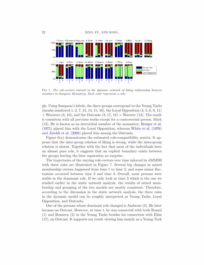
#6, 13, 36, 67, 76). This is the time when Enron filed for bankruptcy.We can also visualize the mixed membership vectors of the network en-

tities and track the trajectory of the mixed membership vector for an indi-vidual as shown in Figure 9. They can help us understand the network as awhole and how each individual evolve in their roles. Based on these exam-ples, we believe dMMSB can provide a useful visual portal for exploring thestories behind Enron.

Apr 2001 #65 Mark Haedicke

4

2

5

3

4

2

5

3

12

3

4

5

6 78

9

1011

12

Fig 9. Left: visualization of mixed membership vectors of network actors in 3-simplexat one time point. Each vertex of the tetrahedron corresponds to a role marked by itsID. A mixed membership vector is represented by a cross whose location and color are theweighted average of its active roles and whose size is proportional to the sum of the weightsfrom the active roles. Right: we track the trajectory of the mixed membership vector foran actor across time. Numbers in italics show time stamps.

5.4. Analysis of Evolving Gene Network as Fruit Fly Aging. In this sec-tion, we study a sequence of gene correlation networks of the fruit flyDrosophila melanogaster estimated at various point of its life cycle. It isknown that over the developmental course of any complex organism, thereexist multiple underlying “themes” that determine the functionalities of eachgene and their relationships to each other, and such themes are dynamicaland stochastic. As a result, the gene regulatory networks at each time pointare context-dependent and can undergo systematic rewiring, rather thanbeing invariant over time. We expect the dMMSB model can capture suchproperties in the time-evolving gene networks of Drosophila melanogaster.

However, experimentally uncovering the topology of gene network at mul-tiple time points as the animal aging is beyond current technology. Herewe used the time-evolving networks of Drosophila Melanogaster reverse-engineered by Kolar et al. (2008) from a genome-wide microarray time seriesof gene expressions using a novel computational algorithm based on ℓ1 regu-larized kernel reweighting regression, which is detailed in a companion paperalso appears in this issue. Altogether, 22 networks at different time pointsacross various developmental stages, namely embryonic stage (1–10 time


point), larval stage (11–13 time point), pupal stage (14–19 time points) andadult stages (20–22 time points), are analyzed. We focused on 588 genesthat are known to be related to developmental process based on their geneontologies.

We plotted the mixed membership vector over 4 roles for each gene asit varies across the developmental cycle (Figure 10). From the time coursesof these mixed membership vectors, we can see that many genes assumevery different roles during different stages of the development. In particu-lar, we see that many genes exhibit sharp transition in terms of their rolesnear the end of embryonic stage. This is consistent with the underlying de-velopmental requirement of Drosophila that the gene interaction networksneed to undergo a drastic reconfiguration to accommodate the new stage oflarval development. Somewhat surprisingly, we found when the number ofroles is set to four, the probability of interacting between different roles isvery small as revealed by the visualization of the role compatibility matrix(Figure 10, lower right). More experiments are needed to examine whetherthis pattern is a true property of the Drosophila gene interactions, or anexperimental artifact (e.g., from accuracy of network reverse engineering; orfrom the smallish number of roles we have chosen to fit the model, whichmight be overly coarse; or from the quality of approximate inference in ahigh-dimensional model).

We selected four genes for further analysis, namely Optix, dorsal (dl),lethal (2) essential for life (l(2)efl) and tolkin (tok). These four genes areamong the highest degree nodes in the network produced by averaging thedynamic networks over time. We want to see how their roles evolve overtime, and therefore we plotted the trajectory of their mixed membershipvector in a 4-d simplex (Figure 11). We can see that the trajectory someof these genes cover a wide area of the 4-d simplex. This is consistent withthe roles of gene Optix and dl as transcriptional factors that participatein many different functions and regulates the expression of a wide range ofother genes. For instance, dl participates in a diverse range of functions suchas anterior/posterior pattern formation, dorsal/ventral axis specification,immune response, gastrulation, heart development; Optix participates innervous system and compound eye development. In contrast, gene tok andl(2)efl are not transcriptional factors and they are currently only knownfor very limited functions: tok is related to axon guidance and wing veinmorphogenesis; l(2)efl related to embryonic and heart development. In ourresults, we found that indeed the role-coorinates of tok are almost invariant,but the trajectory of l(2)efl suggests that it may play more diverse roles thanwhat is current known and deserve further experimental studies.


Fig 10. Changes in mixed membership vectors of all genes, and the visualization for rolecompatibility matrix. The x-axes of each subplot is time, and the y-axes is the weight ofrole-component. Each color stands for a role.


1

2

3

4

Optix

1

2

3

4

dl

1

2

3

4

tok

1

2

3

4

l(2)efl

Fig 11. The trajectories of mixed membership vectors of 4 genes (Optix, dl, tok, l(2)efl).

We further used the mixture membership vectors as features to clustergenes at each time point into 4 clusters (each cluster corresponding to aparticular role-combination pattern), and studied the gene functions in eachrole-combination across time. In other words, we try to provide a func-tional decomposition for each role obtained from the dMMSB model andinvestigate how these roles evolve over time. In particular, we examined 45ontological groups and computed the score enrichment of these biologicalfunctions over random distribution in each role cluster. Figure 12 and Fig-ure 13 demonstrate the results in cluster (i.e., role) 1. The overall patternemerges from our results is that each role consists of genes with a vari-ety of functions, and the functional composition of each role varies acrosstime. However, the distributions over these function groups are very differ-ent for different roles: the most commmon functional groups for genes inrole 1 are related to multicellular organismal development, cuticle develop-ment and pigmentation during development; for the second role, the mostcommon functional groups are gland morphogenisis, heart development, gutdevelopment and ommatidial rotation; for the third role, they are stem cellmaintenance, sensory organ development, central nervous system develop-ment, lymphloid organ development and gland development; for the fourthrole, gastrulation, multicellular organismal development, gut development,stem cell maintenance and regionalization.


Fig 12. Average gene ontology (GO) enrichment score for role 1. The enrichment scorefor a given function is the number of genes labeled as this function. Note that in the plotwe have normalized the score to a range between [0, 1], since we are mainly interested inthe relative count for each GO group. Abbreviations appearing in the figure are: dev. fordevelopment, proc. for process, morph. for morphogenesis, sys. for system.

0 5 10 15 20 25 30 35 40 450

1

0 5 10 15 20 25 30 35 40 450

1

0 5 10 15 20 25 30 35 40 450

1

0 5 10 15 20 25 30 35 40 450

1

0 5 10 15 20 25 30 35 40 450

1

0 5 10 15 20 25 30 35 40 450

1

0 5 10 15 20 25 30 35 40 450

1

0 5 10 15 20 25 30 35 40 450

1

0 5 10 15 20 25 30 35 40 450

1

0 5 10 15 20 25 30 35 40 450

1

0 5 10 15 20 25 30 35 40 450

1

0 5 10 15 20 25 30 35 40 450

1

0 5 10 15 20 25 30 35 40 450

1

0 5 10 15 20 25 30 35 40 450

1

0 5 10 15 20 25 30 35 40 450

1

0 5 10 15 20 25 30 35 40 450

1

0 5 10 15 20 25 30 35 40 450

1

0 5 10 15 20 25 30 35 40 450

1

0 5 10 15 20 25 30 35 40 450

1

0 5 10 15 20 25 30 35 40 450

1

0 5 10 15 20 25 30 35 40 450

1

0 5 10 15 20 25 30 35 40 450

1

Fig 13. Temporal evolution of gene ontology enrichment score for role 1. The time pointsare ordered from left to right, and from top to bottom. The order of the gene ontologygroups are the same as in Figure 12.

6. Discussion. Unlike traditional descriptive methods for studying net-works, which focus on high-level ensemble properties such as degree distri-bution, motif profile, path length, and node clustering, the dynamic mixedmembership stochastic blockmodel proposed in this paper offers an effectiveway for unveiling detailed tomographical information of every actor and rela-tion in a dynamic social or biological network. This methodology has severaldistinctive features in its structure and implementation. First, the social orbiological roles in the dMMSB model are not independent of each other andthey can have their own internal dependency structures; Second, an actorin the network can be fractionally assigned to multiple roles; And third, themixed membership of roles of each actor is allowed to vary temporally. Thesefeatures provides us extra expressive power to better model networks withrich temporal phenomena.

In practice, this increased modelling power also provide better fit to net-works in reality. For instance, the interactions between genes underlying the


developmental course of an organism are centered around multiple themes,such as wing development and muscle development, and these themes aretightly related to each other: without the proper development of musclestructures, the development and functionality of wings can not be fulfiled.As an organism moves along its developmental cycle, the underlying themescan evolve and change drastically. For instance, during embryonic stage ofthe Drosophila, wing development is simply not present and other processessuch as the specification of anterior/posterior axis may be more dominant.Many genes are very versitle in terms of their roles and they differentiallyinteract with different genes depending on the underlying developmentalthemes. Our model is able to capture these various aspects of the dynamicgene interaction networks, and hence leads us a step further in understand-ing the biological processes.

In terms of the algorithm, a key ingredient to glue the three features to-gether is the logistic normal prior for the mixed membership vector. Thisprior is superior to a Dirichlet prior in our context since the off-diagonalentryies of the covariance matrix allow us to code the dependency structurebetween roles, as clearly demonstrated in an earlier work (Ahmed and Xing,2007). Another advantage of the logistic normal prior is that it can be readilycoupled with a state-space model for tracking the evolution of the roles. How-ever, the drawback of the logistic normal prior is that it is not a conjugateprior to the multinomial distribution and therefore additional approxima-tion is needed during learning and inference. For this purpose, we developedan efficient Laplace variantional inference algorithm.

Our algorithm scale quadratically with the number of nodes in the net-work, due to necessity to infer the context-dependent role indicator Z. Itscales quadratically with the number of possible roles, and linearly with thenumber of time steps, which are small comparing to the network size. Theconstant factor typically depends on the stringency of converge test in thevariational EM, and the number of random restarts to alleviate local opti-mum. In our current implementation, we can handle a network with nodes∼ 103 within a day. We have been focusing on developing efficient algo-rithms that enable dynamic tomographic analysis of “meso-level” networks,that is, network with thousands of nodes, rather than “mega” network withmillions of nodes. We feel that this objective is appropriate because formega-networks, such as the bolgsphere and the world wide web, it is theensemble behavior mentioned above that offers more important informationto an investigator who wants to do something with the network, rather thanindividual nodal states. This change of focus with the size of the system canalso be seen in economics and game theory.


There are many dimensions where we can extend our current work. Forinstance, the current model does not explicitly take hubs and cliques of thenetworks into account, and the state-space model does not enforces temporalsmoothness directly over the mixed membership vector but only on its prior.Incorporating these elements will be interesting future research.

APPENDIX A: DERIVATIONS

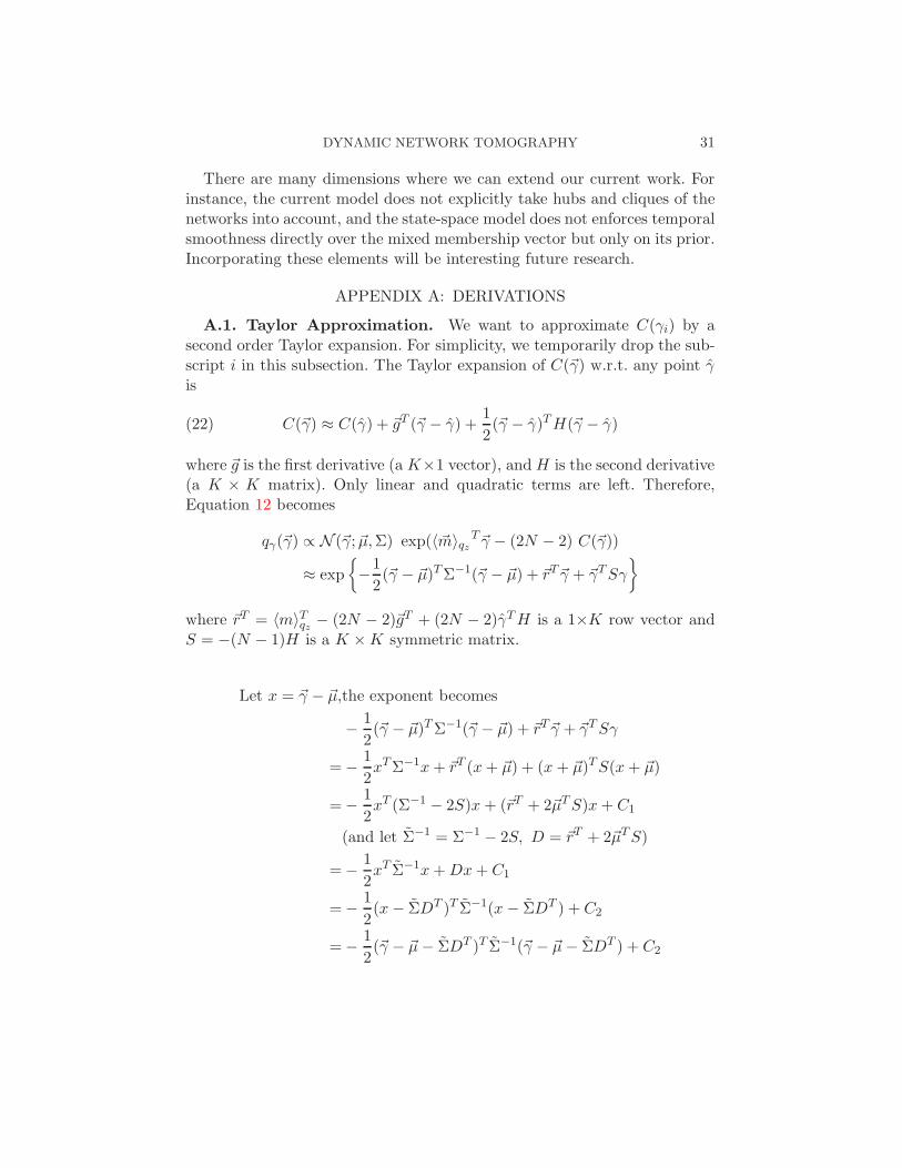
A.1. Taylor Approximation. We want to approximate C(γi) by asecond order Taylor expansion. For simplicity, we temporarily drop the sub-script i in this subsection. The Taylor expansion of C(~γ) w.r.t. any point γis

(22) C(~γ) ≈ C(γ) + ~gT (~γ − γ) +1

2(~γ − γ)T H(~γ − γ)

where ~g is the first derivative (a K×1 vector), and H is the second derivative(a K × K matrix). Only linear and quadratic terms are left. Therefore,Equation 12 becomes

qγ(~γ) ∝ N (~γ; ~µ,Σ) exp(〈~m〉qz

T~γ − (2N − 2) C(~γ))

≈ exp

{

−1

2(~γ − ~µ)T Σ−1(~γ − ~µ) + ~rT~γ + ~γT Sγ

}

where ~rT = 〈m〉Tqz− (2N − 2)~gT + (2N − 2)γT H is a 1×K row vector and

S = −(N − 1)H is a K ×K symmetric matrix.

Let x = ~γ − ~µ,the exponent becomes

−1

2(~γ − ~µ)T Σ−1(~γ − ~µ) + ~rT~γ + ~γT Sγ

=−1

2xT Σ−1x + ~rT (x + ~µ) + (x + ~µ)T S(x + ~µ)

=−1

2xT (Σ−1 − 2S)x + (~rT + 2~µT S)x + C1

(and let Σ−1 = Σ−1 − 2S, D = ~rT + 2~µT S)

=−1

2xT Σ−1x + Dx + C1

=−1

2(x− ΣDT )T Σ−1(x− ΣDT ) + C2

=−1

2(~γ − ~µ− ΣDT )T Σ−1(~γ − ~µ− ΣDT ) + C2


Therefore, Σ = (Σ−1 − 2S)−1 =(

Σ−1 + (2N − 2)H)−1

γ = ~µ + ΣDT = ~µ + Σ(AT + 2S~µ)

= ~µ + Σ(

〈~mi〉qz− (2N − 2)~g + (2N − 2)Hγi − (2N − 2)H~µ

)

where the first and the second derivatives are:

g(γ)k =exp γk

∑

k exp γk

H(γ)kl =I(k = l)∑

k exp γk

−exp γk exp γl

(∑

k exp γk)2

or in short, H = diag(~g)− ~g~gT

A.2. Learning on Logistic-Normal MMSB. The log-likelihood asa function of B can be written as:

l(B) =∑

i,j

log∑

k,l

(

δij,(k,l)βeij

k,l (1− βk,l)(1−eij)

)

+ C0

≥∑

i,j

∑

k,l

δij,(k,l) log(

βeij

k,l (1− βk,l)(1−eij)

)

+ C0

=∑

i,j

∑

k,l

δij,(k,l)

(

eij log βk,l + (1− eij) log(1− βk,l))

+ C0

≡ l∗(B)(23)

∂l∗(B)

∂βk,l

=∑

i,j

∑

k,l

δij,(k,l)

( eij

βk,l

−1− eij

1− βk,l

)

βk,l =

∑

i,j eijδij,(k,l)∑

i,j δij,(k,l)(24)

Jensen’s Inequality is applied in the derivation to get an approximation(more specifically a lower bound) to the log-likelihood which has an analyt-ical solution in finding the maximum point. Setting the derivative to zerogives us an MLE estimator of B based on approximation.


A.3. Learning on dMMSB. Again, we take an approximation of thelog-likelihood, which is more tractable.

l(B) =∑

t

∑

i,j

log∑

k,l

(

δ(t)ij,(k,l)β

e(t)ij

k,l (1− βk,l)(1−e

(t)ij

))

+ C0

≥∑

t

∑

i,j

∑

k,l

δ(t)ij,(k,l) log

(

βe(t)ij

k,l (1− βk,l)(1−e

(t)ij

))

+ C0

=∑

t

∑

i,j

∑

k,l

δ(t)ij,(k,l)

(

e(t)ij log βk,l + (1− e

(t)ij ) log(1− βk,l)

)

+ C0

≡ l∗(B)(25)

The update equation for B is got from maximizing the upper bound of thelog-likelihood.

∂l∗(B)

∂βk,l

=∑

t

∑

i,j

∑

k,l

δ(t)ij,(k,l)

( e(t)ij

βk,l

−1− e

(t)ij

1− βk,l

)

βk,l =

∑

t

∑

i,j e(t)ij δ

(t)ij,(k,l)

∑

t

∑

i,j δ(t)ij,(k,l)

(26)

REFERENCES

A. Ahmed and E. P. Xing. On tight approximate inference of logistic-normal admixturemodel. In Proceedings of the Eleventh International Conference on Artifical Intelligenceand Statistics, 2007.

E. Airoldi, D. Blei, E.P. Xing, and S. Fienberg. A latent mixed membership model forrelational data. In Proceedings of Workshop on Link Discovery: Issues, Approaches andApplications (LinkKDD-2005), The Eleventh ACM SIGKDD International Conferenceon Knowledge Discovery and Data Mining, 2005.

E. M. Airoldi, D. M. Blei, S. E. Fienberg, and E. P. Xing. Mixed membership stochasticblockmodel. Journal of Machine Learning Research, 9:1981–2014, 2008.

J. Aitchison. The statistical analysis of compositional data. Chapman and Hall, New York,NY, USA, 1986.

J. Aitchison and S. M. Shen. Logistic-normal distributions: Some properties and uses.Biometrika, 67(2):261–72, 1980.

A. L. Barabasi and R. Albert. Emergence of scaling in random networks. Science, 286:509–512, 1999.

D. Blei and J. Lafferty. Correlated topic models. In Advances in Neural InformationProcessing Systems 18, 2006a.

D. M. Blei and J. D. Lafferty. Dynamic topic models. In ICML ’06: Proceedings ofthe 23rd international conference on Machine learning, pages 113–120, New York, NY,USA, 2006b. ACM Press. ISBN 1-59593-383-2. .

D. M. Blei, M. I. Jordan, and A. Y. Ng. Hierarchical Bayesian models for applicationsin information retrieval. In J. M. Bernardo, M. J. Bayarri, J. O. Berger, A. P. Dawid,


D. Heckerman, A. F. M. Smith, and M. West, editors, Bayesian Statistics 7, pages25–44. Oxford University Press, 2003a.

D. M. Blei, A. Ng, and M. I. Jordan. Latent Dirichlet allocation. Journal of MachineLearning Research, 3:993–1022, 2003b.

R. Breiger, S. Boorman, and P. Arabie. An algorithm for clustering relational data withapplications to social network analysis and comparison with multidimensional scaling.Journal of Mathematical Psychology, 12:328–383, 1975.

E. Erosheva and S. E. Fienberg. Bayesian mixed membership models for soft clusteringand classification. In C. Weihs and W. Gaul, editors, Classification—The UbiquitousChallenge, pages 11–26. Springer-Verlag, 2005.

E. A. Erosheva, S. E. Fienberg, and J. Lafferty. Mixed-membership models of scientificpublications. Proceedings of the National Academy of Sciences, 97(22):11885–11892,2004.

S. E. Fienberg, M. M. Meyer, and S. Wasserman. Statistical analysis of multiple socio-metric relations. Journal of the American Statistical Association, 80:51–67, 1985.

O. Frank and D. Strauss. Markov graphs. Journal of the American Statistical Association,81:832–842, 1986.

Z. Ghahramani and M.J. Beal. Propagation algorithms for variational Bayesian learning.In Advances in Neural Information Processing Systems 13, 2001.

M. S. Handcock, A. E. Raftery, and J. M. Tantrum. Model-based clustering for socialnetworks. J. R. Statist. Soc. A, 170(2):1–22, 2007.

P. D. Hoff. Bilinear mixed effects models for dyadic data. Technical Report 32, Universityof Washigton, Seattle, 2003.

P. D. Hoff, A. E. Raftery, and M. S. Handcock. Latent space approaches to social networkanalysis. Journal of the American Statistical Association, 97:1090–1098, 2002.

P. Holland, K. B. Laskey, and S. Leinhardt. Stochastic blockmodels: Some first steps.Social Networks, 5:109–137, 1983.

J. Kleinberg. Navigation in a small world. Nature, 845, 2000.M. Kolar, L. Song, A. Ahmed, and E. P. Xing. Estimating time-varying networks. Sub-

mitted to Annals of Applied Statistics, arXiv:0812.5087 [stat.ML], 2008.J. Leskovec, A. Krause, C. Guestrin, C. Faloutsos, J. VanBriesen, and N. Glance. Cost-

effective outbreak detection in networks. In ACM SIGKDD International Conferenceon Knowledge Discovery and Data Mining, 2007.

J. Leskovec, K. Lang, A. Dasgupta, and M. Mahoney. Statistical properties of communitystructure in large social and information networks. In World Wide Web, 2008.

W. Li and A. McCallum. Pachinko allocation: Dag-structured mixture models of topiccorrelations. In ICML ’06: Proceedings of the 23rd international conference on Machinelearning, pages 577–584, New York, NY, USA, 2006. ACM Press. ISBN 1-59593-383-2.URL http://doi.acm.org/10.1145/1143844.1143917.

F. Lorrain and H. C. White. Structural equivalence of individuals in social networks.Journal of Mathematical Sociology, 1:49–80, 1971.

J. Moody and D. R. White. Structural cohesion and embeddedness: A hierarchical conceptof social groups. American Sociological Review, 68:103–127, February 2003.

J. Pritchard, M. Stephens, and P. Donnelly. Inference of population structure using mul-tilocus genotype data. Genetics, 155:945–959, 2000.

S. Sampson. Crisis in a cloister. Unpublished doctoral dissertation, Cornell University.,1969.

P. Sarkar and A. W. Moore. Dynamic social network analysis using latent spacemodels. SIGKDD Explor. Newsl., 7(2):31–40, 2005. ISSN 1931-0145. URLhttp://doi.acm.org/10.1145/1117454.1117459.

http://doi.acm.org/10.1145/1143844.1143917

http://doi.acm.org/10.1145/1117454.1117459


J. Shetty and J. Adibi. The enron email dataset database schema and brief statisticalreport. Technical report, Information Sciences Institute, University of Southern Cali-fornia, 2004.

T. A. B. Snijders. Markov chain monte carlo estimation of exponential random graphmodels. Journal of Social Structure, 2002.

Y. Vardi. Network tomography: Estimating source-destination traffic intensities from linkdata. Journal of the Americian Statistical Association, 91(433):365–377, 1996.

X. Wang and A. McCallum. Topics over time: a non-Markov continuous-time modelof topical trends. In KDD ’06: Proceedings of the 12th ACM SIGKDD internationalconference on Knowledge discovery and data mining, pages 424–433, New York, NY,USA, 2006. ACM Press. ISBN 1-59593-339-5. .

S. Wasserman and P. Pattison. Logit models and logistic regression for social networks:I. an introduction to Markov graphs and p∗. Psychometrika, 61:401–425, 1996.

H. C. White, S. A. Boorman, and R. L. Breiger. Social structure from multiple networks.i. blockmodels of roles and positions. American Journal of Sociology, 81(4):730, 1976.. URL http://www.journals.uchicago.edu/doi/abs/10.1086/226141.

E. P. Xing, M. I. Jordan, and S. Russell. A generalized mean field algorithm for variationalinference in exponential families. In Proceedings of the 19th Annual Conference onUncertainty in AI, 2003.

Address of the authors

5000 Forbes Ave, Wean Hall 4212

Pittsburgh, PA 15213

E-mail: [email protected]@[email protected]

http://www.journals.uchicago.edu/doi/abs/10.1086/226141

mailto:[email protected]



Documents

A State-Space Mixed Membership Blockmodel for Dynamic ...epxing/papers/2010/xing_fu_song_aoas09.pdf · A STATE-SPACE MIXED MEMBERSHIP BLOCKMODEL ... illustrated this model on the