A Standardized PMML Format for Representing Convolutional Neural

Networks with Application to Defect Detection

Max Ferguson1, Yung-Tsun Tina Lee2, Anantha Narayanan3 and Kincho H. Law4

ABSTRACT

Convolutional neural networks are becoming a popular tool for image processing in the

engineering and manufacturing sectors. However, managing the storage and distribution of trained

models is still a difficult task, partially due to the lack of standardized methods for deep neural

network representation. Additionally, the interoperability between different machine learning

frameworks remains poor. This paper seeks to address this issue by proposing a standardized

format for convolutional neural networks, based on the Predictive Model Markup Language

(PMML). A new standardized schema is proposed to represent a range of convolutional neural

networks, including classification, regression and semantic segmentation systems. To demonstrate

the practical application of this standard, a semantic segmentation model, which is trained to detect

casting defects in Xray images, is represented in the proposed PMML format. A high-performance

scoring engine is developed to evaluate images and videos against the PMML model. The utility

of the proposed format and the scoring engine is evaluated by benchmarking the performance of

the defect detection models on a range of different computational platforms.

1-Civil and Environmental Engineering, Stanford University, Y2E2 Building, 473 Via Ortega, Stanford,

CA 94305, USA (Corresponding author); e-mail: maxferg@stanford.edu; https://orcid.org/0000-0003- 4335-5285 2-Systems Integration Division, National Institute of Standards and Technology, 100 Bureau Drive, Gaithersburg,

MD 20899, USA 3- Viterbi School of Engineering, University of Southern California, Los Angeles, CA 90007, USA 4-Civil and Environmental Engineering, Stanford University, Y2E2 Building, 473 Via Ortega, Stanford, CA 94305,

USA

Keywords

Smart Manufacturing, Predictive Model Markup Language, Machine Learning Models, Defect

Detection, Automated Surface Inspection, Convolutional Neural Networks, Standard, Image

Processing

Introduction

Convolutional neural networks (CNNs) are finding numerous real-world applications in

the engineering and manufacturing domains [1]. Recent research has demonstrated that CNNs can

obtain state-of-the-art performance on tasks like casting defect detection [2], anomaly detection in

fibrous materials [3], and classification of waste recycling [4]. In the industry, CNNs are being

used for defect detection [5], weed identification [6], and tracking packages for supply chain

management [7]. However, sharing and deploying trained models still remains a difficult and error-

prone task. In current practice, models are normally saved using a serialization format specific to

the model training framework [8]. While this practice provides a reliable method for saving trained

models, it greatly hinders interoperability between training frameworks and data analysis tools. In

this paper, we seek to address this issue by developing a standardized representation for deep

neural networks, based on the Predictive Model Markup Language (PMML). It is believed that the

proposed format can be useful to the manufacturing industry by:

• Allowing CNN models to be transferred from research laboratories to

manufacturing facilities in a controlled and standardized fashion.

• Enabling legacy PMML software to leverage recent advances in computer vision

technology, through CNN models.

• Providing a reliable way for CNN models to be documented and versioned,

especially in the context of large-scale manufacturing operations.

A standardized representation of a predictive model defines precisely how model inputs

are mapped to model outputs, and often specifies the exact mathematical operations that must be

performed to map an input to an output. The adoption of standardized model representations makes

it easier for a machine learning model to be created, inspected, manipulated and deployed using

different software products. This allows software vendors to develop highly specialized software

products for completing specific tasks on a machine learning model. For example, Tensorflow [8]

can be used to train the model, Netron [9] can be used to test the model, and Google Cloud Platform

[10] can be used to evaluate the model in a production setting.

Many early concerns surrounding CNN-based approaches, such as training stability, large

dataset requirements, and slow training speed have been overcome through algorithmic [11] and

hardware advances [12]. In particular, the discovery of transfer learning has greatly reduced

training dataset requirements, allowing powerful models to be trained with relatively small datasets

[2, 13]. However, both transfer learning and hardware acceleration bring additional complexity to

the model training and deployment process. Transfer learning requires the model to be trained on

at least two datasets, meaning that an intermediate representation for the model is almost essential.

Similarly, with the widespread adoption of hardware acceleration, it is becoming common to train

and evaluate the models on different hardware devices. Again, a reliable representation of the

machine learning model is essential for transferring a machine learning model from one

computational platform to another.

The remainder of the paper is organized as follows: The Background section provides an

introduction to many concepts that are expanded on throughout the paper. The Related Work

section describes related work in the field of standardized neural network models. The PMML for

CNN section describes the proposed extensions to the PMML specification. The Manufacturing

Defect Segmentation section describes how the proposed PMML format is used to represent an

Xray defect detection model. The paper is concluded with a brief discussion and conclusion.

Background

This paper proposes a new standardized format for representing deep neural networks in

PMML. Before the PMML representation is presented, this section introduces many of the topics

that are fundamental to the discussion and motivation of such a standardization.

PMML

PMML is an extensible language that enables the definition and sharing of predictive

models between applications [14]. PMML provides a clean and standardized interface between the

software tools that produce predictive models, such as statistical or data mining systems, and the

consumers of models, such as applications that depend upon embedded analytics [15]. Once a

machine learning model has been trained in an environment like Python, MATLAB, or R, it can

be saved as a PMML file. The PMML file can then be moved to a production environment, such

as an embedded system or a cloud server. A scoring engine in the production environment can

parse the PMML file and use it to generate predictions for new unseen data points.

PMML is based on the Extensible Markup Language (XML). XML is a markup language

that defines a set of rules for encoding documents in a format that is both human-readable and

machine-readable. Simple XML elements contain an opening tag, a closing tag, and some content.

The opening tag begins with a left angle bracket (<), followed by an element name that contains

letters and numbers, and finishes with a right angle bracket (>). Closing tags follow a similar

format, but have a forward slash (/) before the right angle bracket. In PMML, each element either

describes a property of the model or provides metadata about the model. An XML schema

describes the elements and attributes that are permissible in an XML file.

Neural Networks

Feedforward neural networks are the quintessential deep learning models. Neural networks

"learn" to perform tasks by considering examples, generally without being programmed with any

task-specific rules. For example, a neural network could be trained to identify images that contain

manufacturing defects by exposing it to example images that have been manually labeled as

“defective” or “not defective”. Such neural networks are generally trained with little prior

knowledge about manufacturing parts or defects. Instead, neural networks automatically generate

identifying characteristics from the dataset that they are trained on. While neural networks were

loosely inspired by neuroscience, it is best to think of feedforward networks as function

approximation machines that are designed to achieve statistical generalization.

The goal of a feedforward network is to approximate some function 𝑓∗. For example, for a

classifier, 𝑦 = 𝑓∗(𝒙) that maps an input 𝒙 to a category 𝑦, a feedforward network defines a

mapping 𝑦 = 𝑓(𝒙; 𝜽) and learns the value of the parameters 𝜽 that result in the best function

approximation. These models are called feedforward because information flows through the

function being evaluated from 𝒙, through the intermediate computations used to define 𝑓, and

finally to the output 𝑦. There are no feedback connections in which outputs of the model are fed

back into itself. Feedforward neural networks are called networks because they are typically

represented by composing together many different functions. The neural network model is

associated with a directed acyclic graph describing how the functions are composed together [16].

For example, we might have three functions 𝑓1, 𝑓2, and 𝑓3 connected in a chain, to form 𝑓(𝒙) =

𝑓3 (𝑓2(𝑓1(𝒙))). These chain structures are the most commonly used structures of neural networks.

In this case, 𝑓1 is called the first layer of the network, 𝑓2 is called the second layer, and so on. The

overall length of the chain gives the depth. The final layer of a feedforward network is called the

output layer. During neural network training, we drive 𝑓(𝒙) to match 𝑓∗(𝒙). The training data

provides us with noisy, approximate examples of 𝑓∗(𝒙) evaluated at different training points. Each

example 𝒙 is accompanied by a label y ≈ 𝑓∗(𝒙). The training examples specify directly what the

output layer must do at each point 𝒙, and produces a value that is close to 𝑦. The output of the

other layers is not directly specified by the learning algorithm or training data. Instead, the learning

algorithm must decide how to use these layers to best implement an approximation of 𝑓∗(𝒙).

Convolutional Neural Networks

Convolutional neural networks, or CNNs, are a specialized kind of neural network for

processing data that has a known grid-like topology [16]. Although this work focuses on the

application of CNNs to image data, CNNs can operate on a variety of other data types, including

time series and point cloud data. In a CNN, pixels from each image are converted to a featurized

representation through a series of mathematical operations. Input images are represented as an

order 3 tensor 𝐼 ∈ ℝ𝐻×𝑊×𝐷 with height 𝐻, width 𝑊, and depth 𝐷 color channels [17]. This

representation is modified by a number of hidden layers until the desired output is achieved. There

are several layer types which are common to most modern CNNs, including convolution, pooling

and dense layer types. A convolution layer is a function 𝑓𝑖(𝒙𝑖; 𝜽𝑖) that convolves one or more

parameterized kernels with the input tensor, 𝒙𝑖. Suppose the input 𝒙𝒊 is an order 3 tensor with size

𝐻𝑖 × 𝑊𝑖 × 𝐷𝑖. A convolution kernel is also an order 3 tensor with size 𝐻𝑘 × 𝑊𝑘 × 𝐷𝑖, where

𝐻𝑘 × 𝑊𝑘 is the spatial size of the kernel. The kernel is convolved with the input by taking the dot

product of the kernel with the input at each spatial location in the input. By convolving certain

types of kernels with the input image, it is possible to obtain meaningful outputs, such as the image

gradients. In most modern CNN architectures, the first few convolutional layers extract features

like edges and textures in an image. Convolutional layers deeper in the network can extract features

that span a greater spatial area of the image, such as object shapes. Pooling layers are used to

reduce the spatial size of a feature map. Pooling involves applying a pooling operation, much like

a filter, to the feature map. The size of the pooling operation is smaller than the size of the feature

map; it is common to apply a pooling operation with a size of 2×2 pixels and a stride of 2 pixels.

Dense layers apply an affine transformation to the input vector, and in many cases, also apply an

elementwise nonlinear function. They are generally used to learn a mapping between a flattened

convolutional layer feature map and the target output of the CNN.

Dataflow Graphs

Many machine learning software frameworks represent neural networks as dataflow

graphs. In a dataflow graph, the nodes represent units of computation, and the edges represent the

data consumed or produced by a computation. A dataflow graph for a small neural network is

shown in FIG 1. Each layer in the neural network is represented as a node in the dataflow graph.

The graph edges specify the inputs to each layer. Representing a CNN in this form allows the

underlying software framework to optimize the training and execution of the neural network

through increased parallelism and compiler-generated optimizations. One way of creating a

persistent representation of a neural network is to save the dataflow graph in a standardized

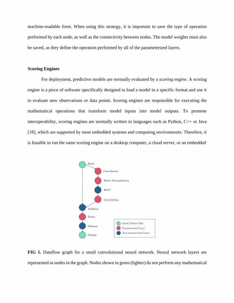
machine-readable form. When using this strategy, it is important to save the type of operation

performed by each node, as well as the connectivity between nodes. The model weights must also

be saved, as they define the operation performed by all of the parameterized layers.

Scoring Engines

For deployment, predictive models are normally evaluated by a scoring engine. A scoring

engine is a piece of software specifically designed to load a model in a specific format and use it

to evaluate new observations or data points. Scoring engines are responsible for executing the

mathematical operations that transform model inputs into model outputs. To promote

interoperability, scoring engines are normally written in languages such as Python, C++ or Java

[18], which are supported by most embedded systems and computing environments. Therefore, it

is feasible to run the same scoring engine on a desktop computer, a cloud server, or an embedded

FIG 1. Dataflow graph for a small convolutional neural network. Neural network layers are

represented as nodes in the graph. Nodes shown in green (lighter) do not perform any mathematical

operations on the input tensor. Nodes shown in red have learnable parameters, whilst nodes shown

in blue (darker) do not have any learnable parameters.

device, without modifying the scoring engine code. With the adoption of more complex models,

such as deep neural networks, it is becoming common-practice to evaluate models on hardware-

accelerated scoring engines. Hardware acceleration generally increases the throughput of the

scoring engine, decreases the model prediction time, and decreases power consumption for large-

scale computational tasks.

Related Works

In current deep learning practice, there are many different formats for storing machine

learning models. The existing neural network representations can be classified as framework-

specific or framework-agnostic. Framework-specific representations, such as the PyTorch model

format [19], are tightly bound to a particular machine learning framework or programming

language. However, these framework-specific formats often lack compatibility with machine

learning frameworks other than the framework for which they were designed. Framework-agnostic

formats like PMML or Open Neural Network Exchange (ONNX) [20] encourage software

interoperability, but tend to be more difficult to design and implement. This section reviews

existing methods and standards for representing neural network models; the purpose is to highlight

the prevalent framework-agnostic and framework-specific representations.

PyTorch

PyTorch is an open source machine learning library for Python that is commonly used for

applications like image processing and natural language processing [19]. It is primarily developed

by Facebook's artificial-intelligence research group. PyTorch models are exported to a binary

format using the Python Pickle protocol. While this approach provides a seamless method of

persisting PyTorch models, it greatly hinders interoperability. In particular, relying on the Pickle

object serialization format makes it difficult to transfer PyTorch models to other computing

environments that do not support the Python runtime. PyTorch allows a neural network graph to

be represented using the JavaScript Object Notation (JSON). The JSON format is supported by

most common programming languages, making it an attractive option for saving a neural network

architecture. However, as PyTorch does not export the model weights to JSON there is currently

no way to fully recover a trained model from the JSON representation.

TensorFlow

TensorFlow is an open source software library for high performance numerical

computation. Its flexible architecture allows easy deployment of computation across a variety of

platforms [8]. TensorFlow provides options for saving model weights alone or saving the dataflow

graph and model weights. The dataflow graph can be exported to a binary file using the Protocol

Buffer format. A separate Application Programming Interface (API) also provides the option to

save the model weights in the Hierarchical Data format (HDF5) binary format. Alternatively, the

entire model can be exported using a custom binary format that is based on HDF5 and Protocol

Buffers. Google has developed tools to allow these models to be evaluated in other programming

languages, such as JavaScript or C++. However, without a clear open source specification for the

model representation, there is still very limited interoperability between TensorFlow and other

predictive modelling tools.

ONNX

The Open Neural Network Exchange (ONNX) format is a community project created by

Facebook and Microsoft [20]. ONNX provides a definition of an extensible computation graph

model, as well as definitions of built-in operators and standard data types. Each computational

dataflow graph is structured as a list of nodes that form an acyclic graph. Nodes have one or more

inputs and one or more outputs. Each node is a call to an operator. The graph also has metadata to

help document its purpose, author, etc. Operators are implemented external to the graph, but the

set of built-in operators are portable across frameworks. Every framework supporting ONNX will

provide implementations of these operators on the applicable data types. ONNX currently supports

a wide range of models, including feedforward neural networks and CNNs. Neural network

architectures for image classification, image segmentation, object detection, and face recognition,

among several others, are supported. There is experimental support for recurrent neural networks

(RNNs). Fundamentally, ONNX supports the representation of neural networks at a lower-level

than the proposed PMML representation to be discussed in this paper. In some cases, this makes

the ONNX standard more suitable than PMML for highly complex neural network architectures

that rely on abnormal mathematical transformations or non-standardized neural network layers.

On the other hand, for the ONNX standard, this added complexity also makes it more difficult to

implement fully-compliant scoring engines or model converters. Therefore, we believe that is

possible for PMML and ONNX to coexist, with PMML being used to represent widely-used model

architectures like residual networks [21], and ONNX being used to represent more complex

research-grade neural network models.

PMML

PMML is a high-level XML-based language designed to represent data-mining and

predictive models [14], such as linear regression models or random forests [14]. PMML does not

control the way that the model is trained, it is purely a standardized way to represent the trained

model. PMML is designed to be human-readable and uses a predefined set of model types and

parameters to describe each model. This contrasts with the approach employed in formats like

Portable Format for Analytics (PFA) [22] and ONNX [20], which represent models as a complex

graph of mathematical operations. PMML 3.0 introduced a standard format for feedforward neural

network models [22]. However, PMML documents conforming to this standard explicitly define

every neural network connection using XML. Representing deep feedforward neural networks in

this manner is impractical as deep neural networks often have between 𝑂(106) to 𝑂(109)

connections [21]. Instead, the work described herein proposes a format that represents each layer

of the neural network using XML, rather than representing every dense connection with XML.

The benefit of this approach is that a deep neural network can be represented in only a few thousand

lines of XML, whilst the standard remains flexible enough to represent most commonly used

architectures. A related work described how PMML can be used to represent CNN classification

models [23]. This paper expands on that work by adding support for many other neural network

architectures, including those used for semantic segmentation, object localization and object

detection.

PMML for Convolutional Neural Networks

PMML supports a large number of model types, including random forest [14], Gaussian

process regression [24], and linear and feedforward neural networks [22]. The main contribution

of this section is a specification for a new PMML element, namely the DeepNetwork element. The

remainder of this section explains how the proposed DeepNetwork element can be used to describe

a CNN model. FIG 2 shows the general structure of a DeepNetwork PMML document, which

includes four basic elements, namely, header, data dictionary, data transformation, and the deep

network model [14]. The XML schema for the DeepNetwork element precisely describes the

DeepNetwork element and related XML elements. The XML schema is made publicly available

on Github [25]. The following briefly describes the PMML structure and the layers that are

intended in the proposed PMML scheme.

PMML STRUCTURE

The Header element provides a general description of the PMML document, including

name, version, timestamp, copyright, and other relevant information for the model-development

environment. The DataDictionary element contains the data fields and their types, as well as the

admissible values for the input data. Data transformation is performed using the optional

TransformationDictionary or LocalTransformations element. These elements describe the

mapping of the data, if necessary, into a form usable by the mining or predictive model. The last

element in the general structure contains the definition and description of the predictive model.

The element is chosen among a list of models defined in the PMML standard. We propose the

DeepNetwork model element as a new element for representing deep neural network models in

PMML.

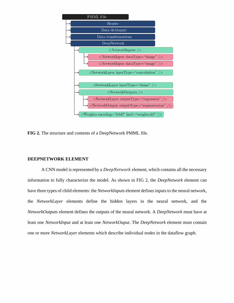
DEEPNETWORK ELEMENT

A CNN model is represented by a DeepNetwork element, which contains all the necessary

information to fully characterize the model. As shown in FIG 2, the DeepNetwork element can

have three types of child elements: the NetworkInputs element defines inputs to the neural network,

the NetworkLayer elements define the hidden layers in the neural network, and the

NetworkOutputs element defines the outputs of the neural network. A DeepNetwork must have at

least one NetworkInput and at least one NetworkOuput. The DeepNetwork element must contain

one or more NetworkLayer elements which describe individual nodes in the dataflow graph.

FIG 2. The structure and contents of a DeepNetwork PMML file.

NEURAL NETWORK LAYERS

In the proposed PMML standard extension, a deep neural network is represented as a

directed acyclic graph. Each node in the graph represents a neural network layer. Graph edges

describe the connections between neural network layers. As shown in FIG 2, the NetworkLayer

element is used to define the node in the proposed DeepNetwork PMML extension. Similarly, the

NetworkInputs element is used to describe the input to the neural network. The layerName attribute

of each NetworkLayer and NetworkInputs elements uniquely identifies each neural network layer.

As shown in FIG 3, it is possible to connect layers by specifying the inputs to each layer.

Specifically, a NetworkLayer can have a child InboundNodes element which defines inputs to the

layer. If the InboundNodes child is not present, then it is assumed that the layer does not have any

inputs.

Most modern neural network architectures are composed from a set of standardized layer

types, in which each performs an operation on the feature representation. In this section, we

FIG 3. Two connected nodes in a neural network graph, represented using the DeepNetwork

PMML format.

introduce PMML definitions for many of these layer types. Convolution layers convolve a

parameterized filter with the feature representation. Pooling layers [16] reduce the spatial

dimension of the feature representation by apply a sliding maximum or average operator across

the representation. Batch normalization [11] layers aim to standardize the mean and variance of

input tensors, to avoid internal covariate shift. Nonlinearity layers, such as rectified linear units

(ReLU), sigmoid, or tanh introduce nonlinearity to the neural network, allowing the neural network

to represent a much larger set of functions [16]. Many of these layers have parameters 𝜽𝑖 that are

learned during the training process. Convolution, batch normalization and fully connected layers

generally have learnable parameters, whilst pooling and nonlinearity layers typically do not have

any learnable parameters. The learnable parameters for a neural network are generally referred to

collectively as model weights. FIG 4 shows a summary of the layers currently defined in the

PMML format.

Convolution Layer

The convolution layer convolves a convolutional kernel with the input tensor [16]. As

shown in FIG 4, the convolution layer is represented using a NetworkLayer element with layerType

set to Conv2D. A NetworkLayer with the Conv2D layer type must contain a ConvolutionalKernel

child element, which describes the properties of the convolutional kernel. The cardinality of the

convolutional tensor must be equal to that of the input tensor. The size of the convolutional kernel

is governed by the parameter KernelSize child element, and the stride is governed by the parameter

KernelStrides. An activation function can be optionally applied to the output of this layer.

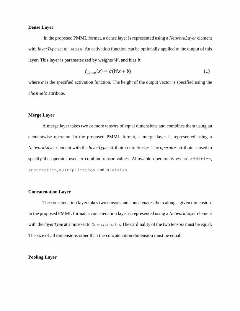
Dense Layer

In the proposed PMML format, a dense layer is represented using a NetworkLayer element

with layerType set to Dense. An activation function can be optionally applied to the output of this

layer. This layer is parameterized by weights 𝑊, and bias 𝑏:

𝑓𝑑𝑒𝑛𝑠𝑒(𝑥) = 𝜎(𝑊𝑥 + 𝑏) (1)

where 𝜎 is the specified activation function. The height of the output vector is specified using the

𝑐ℎ𝑎𝑛𝑛𝑒𝑙𝑠 attribute.

Merge Layer

A merge layer takes two or more tensors of equal dimensions and combines them using an

elementwise operator. In the proposed PMML format, a merge layer is represented using a

NetworkLayer element with the layerType attribute set to Merge. The operator attribute is used to

specify the operator used to combine tensor values. Allowable operator types are addition,

subtraction, multiplication, and division.

Concatenation Layer

The concatenation layer takes two tensors and concatenates them along a given dimension.

In the proposed PMML format, a concatenation layer is represented using a NetworkLayer element

with the layerType attribute set to Concatenate. The cardinality of the two tensors must be equal.

The size of all dimensions other than the concatenation dimension must be equal.

Pooling Layer

Pooling layers apply a pooling operation over a single tensor. In the proposed PMML

format, a max pooling layer is represented using a NetworkLayer element with the layerType

attribute set to MaxPooling2D. An average pooling layer is represented using a NetworkLayer

element with the layerType attribute set to AveragePooling2D. The width of the pooling kernel

is governed by the PoolSize child element, and the stride is governed by the parameter PoolStrides

child element.

Global Pooling Layer

Global pooling layers apply a pooling operation across all spatial dimensions of the input

tensor. In the proposed PMML format, a global max pooling layer is represented using a

NetworkLayer element with the layerType attribute set to GlobalMaxPooling2D. A global

average pooling layer is represented using a NetworkLayer element with the layerType attribute

set to GlobalAveragePooling2D. Both of these global pooling layers return a tensor that has

size (𝑏𝑎𝑡𝑐ℎ_𝑠𝑖𝑧𝑒, 𝑐ℎ𝑎𝑛𝑛𝑒𝑙𝑠).

Depthwise Convolution Layer

The depthwise convolution layer convolves a convolutional filter with the input, keeping

each channel separate. In the regular convolution layer, convolution is performed over multiple

input channels. The depth of the filter is equal to the number of input channels, allowing values

across multiple channels to be combined to form the output. Depthwise convolutions keep each

channel separate - hence the name depthwise. In the proposed PMML format, a depthwise

convolution layer is represented using a NetworkLayer element with the layerType attribute set to

DepthwiseConv2D.

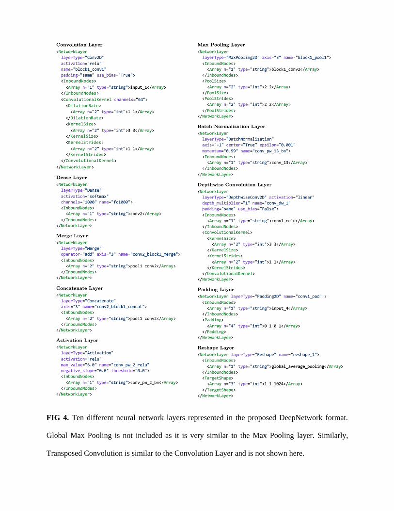
FIG 4. Ten different neural network layers represented in the proposed DeepNetwork format.

Global Max Pooling is not included as it is very similar to the Max Pooling layer. Similarly,

Transposed Convolution is similar to the Convolution Layer and is not shown here.

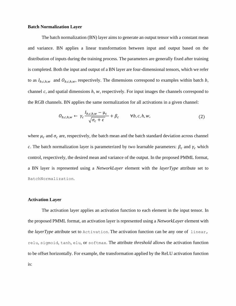
Batch Normalization Layer

The batch normalization (BN) layer aims to generate an output tensor with a constant mean

and variance. BN applies a linear transformation between input and output based on the

distribution of inputs during the training process. The parameters are generally fixed after training

is completed. Both the input and output of a BN layer are four-dimensional tensors, which we refer

to as 𝐼𝑏,𝑐,ℎ,𝑤 and 𝑂𝑏,𝑐,ℎ,𝑤, respectively. The dimensions correspond to examples within batch 𝑏,

channel 𝑐, and spatial dimensions ℎ, 𝑤, respectively. For input images the channels correspond to

the RGB channels. BN applies the same normalization for all activations in a given channel:

𝑂𝑏,𝑐,ℎ,𝑤 ← 𝛾𝑐

𝐼𝑏,𝑐,ℎ,𝑤 − μc

√𝜎𝑐 + 𝜖 + 𝛽𝑐 ∀𝑏, 𝑐, ℎ, 𝑤, (2)

where 𝜇𝑐 and 𝜎𝑐 are, respectively, the batch mean and the batch standard deviation across channel

𝑐. The batch normalization layer is parameterized by two learnable parameters: 𝛽𝑐 and 𝛾𝑐 which

control, respectively, the desired mean and variance of the output. In the proposed PMML format,

a BN layer is represented using a NetworkLayer element with the layerType attribute set to

BatchNormalization.

Activation Layer

The activation layer applies an activation function to each element in the input tensor. In

the proposed PMML format, an activation layer is represented using a NetworkLayer element with

the layerType attribute set to Activation. The activation function can be any one of linear,

relu, sigmoid, tanh, elu, or softmax. The attribute threshold allows the activation function

to be offset horizontally. For example, the transformation applied by the ReLU activation function

is:

𝒙 ← 𝒙 − 𝑡 (3)

𝑓𝑟𝑒𝑙𝑢(𝒙) = min(max(𝑎, 𝑎𝒙) , 𝛾) (4)

where 𝑎 is the value of the negative_slope attribute, 𝑡 is the value of the threshold attribute, and 𝛾

is the value of the max_value attribute. If the max_value attribute is not supplied, then 𝛾 is assumed

to be infinity.

Padding Layer

A padding layer pads the spatial dimensions of a tensor with a constant value, often zero.

This operation is commonly used to increase the size of oddly shaped layers, to allow dimension

reduction in subsequent layers. In the proposed PMML format, a padding layer is represented using

a NetworkLayer element with the layerType attribute set to Padding2D.

Reshape Layer

A reshape layer reshapes the input tensor. The number of values in the input tensor must

equal the number of values in the output tensor. The first dimension is not reshaped as this is

commonly the batch dimension. In the proposed PMML format, a padding layer is represented

using a NetworkLayer element with the layerType attribute set to Reshape. The flatten layer is a

variant of the reshape layer, that flattens the input tensor such that the output size is

(𝑏𝑎𝑡𝑐ℎ_𝑠𝑖𝑧𝑒, 𝑛) where 𝑛 is the number of values in the input tensor. In the proposed PMML

format, a flatten layer is represented using a NetworkLayer element with the layerType attribute

set to Flatten.

Transposed Convolution

Transposed convolutions, also called deconvolutions, arise from the desire to use a

transformation going in the opposite direction of a normal convolution, for example to increase

the spatial dimensions of a tensor. They are commonly used in CNN decoders, which progressively

increase the spatial size of the input tensor. In the PMML CNN format, a transposed convolution

layer is represented using a NetworkLayer element with the layerType attribute set to

TransposedConv2D.

NEURAL NETWORK OUTPUT

CNNs are commonly used for image classification, segmentation, regression, and object

localization. To be widely applicable, the PMML CNN standard should support all of these output

types. The proposed standard should also support multiple outputs types such that it can, for

example, predict the age and gender of a person from an image. The NetworkOutputs element is

used to define the outputs of a deep neural network. Each output is defined using the

NetworkOutput element. Several examples of neural network output definitions are provided in

FIG 5.

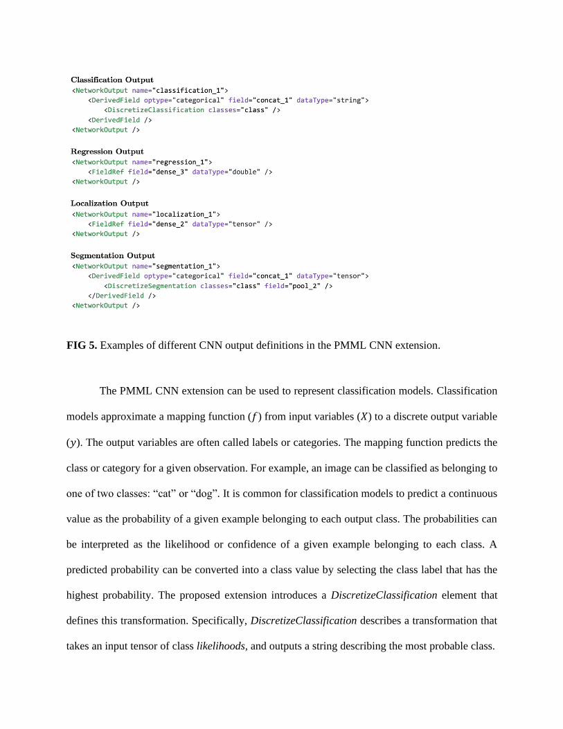
The PMML CNN extension can be used to represent classification models. Classification

models approximate a mapping function (𝑓) from input variables (𝑋) to a discrete output variable

(𝑦). The output variables are often called labels or categories. The mapping function predicts the

class or category for a given observation. For example, an image can be classified as belonging to

one of two classes: “cat” or “dog”. It is common for classification models to predict a continuous

value as the probability of a given example belonging to each output class. The probabilities can

be interpreted as the likelihood or confidence of a given example belonging to each class. A

predicted probability can be converted into a class value by selecting the class label that has the

highest probability. The proposed extension introduces a DiscretizeClassification element that

defines this transformation. Specifically, DiscretizeClassification describes a transformation that

takes an input tensor of class likelihoods, and outputs a string describing the most probable class.

FIG 5. Examples of different CNN output definitions in the PMML CNN extension.

The proposed PMML extension can also be used to represent models which return one or

more continuous values. This type of model is commonly referred to as a regression model.

Formally, regression models approximate a mapping function (𝑓) from input variables (𝑋) to a

continuous output variable (𝑌). A continuous output variable is a real-value, such as an integer or

floating point value, or a tensor of continuous values. These are often quantities, such as amounts

and sizes. The existing FieldRef PMML element is used to define regression models. If a FieldRef

is contained in a NetworkOuput then it returns a copy of any specified tensor in the neural network.

If the FieldRef has a double datatype, then it converts single element tensors to a single double

value.

Deep neural networks are also commonly used for object localization. Object localization

is the problem of predicting the location of an object in an image. A localization model will often

return object coordinates in the form (𝑥1, 𝑦1, 𝑥2, 𝑦2) that describe the corners of the predicted

bounding box. This type of model can be simply represented as regression model that outputs four

continuous variables. Alternatively, this model can be represented as a regression model that

returns a tensor containing four continuous values.

Semantic segmentation is one of the fundamental tasks in computer vision. In semantic

segmentation, the goal is to classify each pixel of the image in a specific category. Formally,

semantic segmentation models approximate a mapping function (𝑓) from an input image (𝐼 ∈

ℝ𝑊×𝐻×𝐶) to a tensor of object classes (𝑌 ∈ ℝ𝑊×𝐻). Most modern neural network architectures

learn a mapping between the input image and a tensor that describes the class likelihood for each

pixel 𝑃 ∈ ℝ𝑊×𝐻×𝑁, where 𝑁 is the number of predefined classes. The final step is to select the

class with the largest likelihood for each pixel. The proposed PMML extension introduces a

DiscretizeSegmentation element that defines this transformation. Specifically,

DiscretizeSegmentation describes a transformation that takes an input tensor 𝑃, and outputs a

tensor containing the most likely pixel classes.

Manufacturing Defect Segmentation

In this section, we show how the proposed PMML format can be used to facilitate transfer

learning in a defect segmentation task. CNNs have been particularly successful for detecting

manufacturing defects using camera or Xray images [1, 2, 26]. The goal of this section is to develop

classifier that can segment each pixel of an Xray image into one of three classes: manufacturing

part, manufacturing defect and background. The background class aims to capture the part of the

image which does not contain any manufacturing parts. In this way, the algorithm can identify the

shape of the scanned part, in addition to identifying any defects in the part. Four pretrained image

segmentation models are converted to the PMML format, allowing them to be easily loaded into

machine learning frameworks such as Keras, TensorFlow or PyTorch. Each model is then

finetuned on the GDXray casting defect dataset. The finetuned models are exported to the proposed

PMML format and made publicly available. Finally, the PMML models are loaded onto a high-

performance TensorFlow scoring engine to demonstrate how the model could be used in a

manufacturing environment.

GDXRAY DATASET

The GDXRay dataset is a collection of annotated Xray images [27]. The Castings series of

this dataset contains 2727 Xray images mainly from automotive parts, including aluminum wheels

and knuckles. The casting defects in each image are labeled with tight fitting bounding-boxes. The

size of the images in the dataset ranges from 256 256 pixels to 768  572 pixels. The GDXray

dataset has been used by many researchers as a standard benchmark for defect detection and

segmentation [23, 28]. In this work, another segmentation label is added to the dataset that

separates manufacturing parts from empty space or unrelated objects in the Xray scan. The new

labels are generated in a semi-automated fashion, using traditional computer vision techniques

including median filtering and k-means clustering. All labels are then manually validated and

edited.

In previous work, we trained CNN models for defect instance segmentation [1], defect

detection [2] and tile-based defect classification [23], all using the GDXray dataset. In defect

detection, the goal is to place a bounding box around each defect in the image. In defect instance

segmentation, the goal is to identify which image pixels belong to each defect. Finally, in tile-

based defect classification, the goal is to simply predict whether a defect exists somewhere in an

image. In a practical sense, defect instance segmentation models are the most useful, as they predict

the exact pixel location of each defect. However, instance segmentation models are notoriously

difficult to train and slow to evaluate, when compared to pixel segmentation models. Therefore,

we choose to train a pixel segmentation model. In the case where defects are not touching, the

pixel segmentation and instance segmentation models will essentially produce the same type of

output. The popular U-Net architecture is chosen for defect segmentation, as it has be successfully

applied to many similar problems in biomedical [29] and engineering applications [30]. The U-

Net architecture consists of an encoder and a decoder. The encoder is a CNN that gradually reduces

the spatial size of the input image whilst increasing the number of channels. It is common practice

to use a portion of a classification model, such as ResNet-50, for the U-Net encoder. The decoder

is a CNN that performs the opposite transformation on the image, gradually increasing the spatial

size whilst reducing the number of channels. The output of the U-Net model is a tensor that

describes the class likelihood for each pixel. The predicted class can be obtained by finding the

maximum score for each pixel.

TRAINING

The U-Net architecture is chosen as the primary architecture for semantic segmentation of

manufacturing defects. Experiments are conducted using the U-Net architecture with four different

backbone networks, namely VGG-16, ResNet-50, MobileNet and DenseNet-121. The GDXray

Castings dataset is divided into training and testing datasets, using the same split as described

previously in an earlier work [2]. Images that do not contain any defects are discarded from the

training set. Image augmentation is used extensively to prevent overfitting. During training, images

are randomly sampled from the training set and padded with black pixels, such that they have a

height and width of 384 pixels or larger. Each image is randomly cropped to a size of 384 384

pixels. The image is then rotated 90 degrees, horizontally flipped, or vertically flipped with a

probability of 0.5. Rotating or flipping an image in GDXray Casting dataset produces an image

that could be recreated using the same test apparatus, validating this augmentation procedure.

Additionally, elastic deformation [31] and brightness transformations are applied to the images.

Elastic deformation changes the apparent shape of the manufactured part, without producing a

unreasonable image. In general, the defects in the GDXray Castings series can easily be hidden

when scaling, distorting or adding noise to the images [1]. Hence, no blurring or random noise is

added to the images, and only a small amount of elastic deformation is applied. The U-Net models

are all trained for 20 Epochs on the GDXray dataset using the Adam optimizer [32], with a batch

size of 16 and an initial learning rate of 0.01.

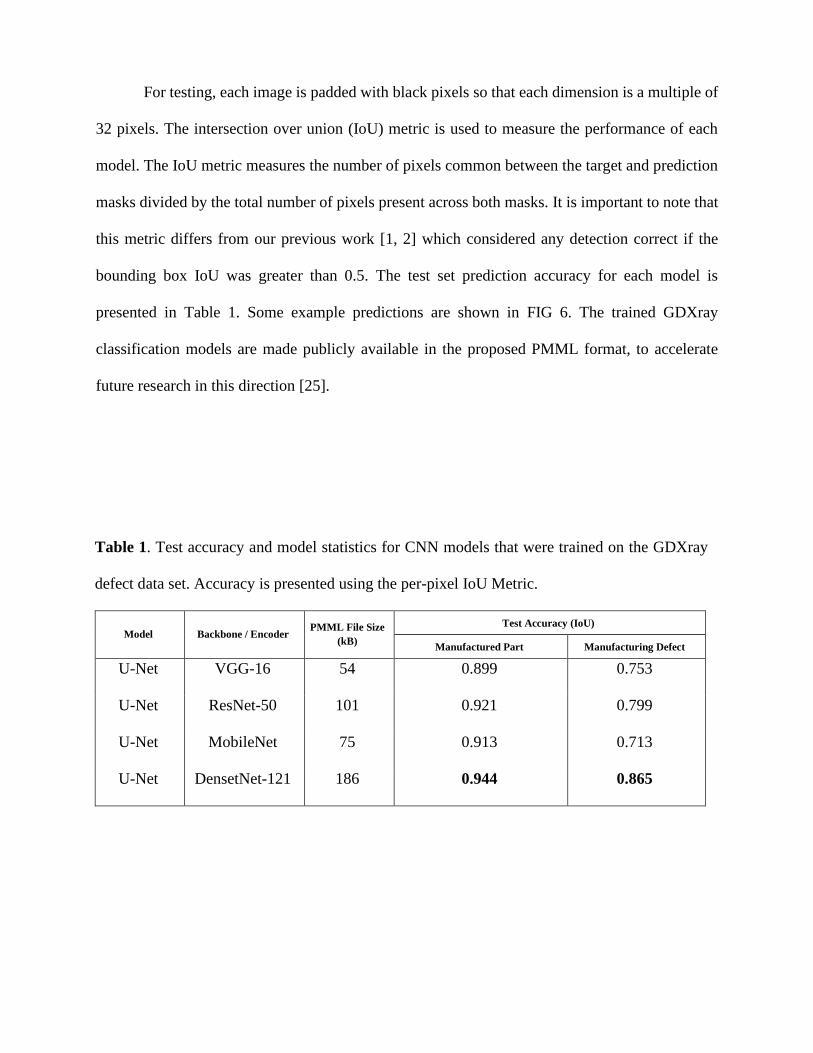
For testing, each image is padded with black pixels so that each dimension is a multiple of

32 pixels. The intersection over union (IoU) metric is used to measure the performance of each

model. The IoU metric measures the number of pixels common between the target and prediction

masks divided by the total number of pixels present across both masks. It is important to note that

this metric differs from our previous work [1, 2] which considered any detection correct if the

bounding box IoU was greater than 0.5. The test set prediction accuracy for each model is

presented in Table 1. Some example predictions are shown in FIG 6. The trained GDXray

classification models are made publicly available in the proposed PMML format, to accelerate

future research in this direction [25].

Table 1. Test accuracy and model statistics for CNN models that were trained on the GDXray

defect data set. Accuracy is presented using the per-pixel IoU Metric.

Model Backbone / Encoder PMML File Size

(kB)

Test Accuracy (IoU)

Manufactured Part Manufacturing Defect

U-Net VGG-16 54 0.899 0.753

U-Net ResNet-50 101 0.921 0.799

U-Net MobileNet 75 0.913 0.713

U-Net DensetNet-121 186 0.944 0.865

The application of transfer learning has been shown to be beneficial on the GDXray dataset

[1]. In transfer learning, a model is first trained on a large dataset, like the ImageNet dataset. The

model is then fine-tuned on a domain-specific task. In many cases, knowledge gained from the

original task can improve the performance on the second task. In this work, transfer learning is

applied as follows: Pretrained models are obtained for the U-Net backbone networks, namely

VGG-16, ResNet-50, MobileNet and DenseNet-121. These models are converted to the PMML

CNN format using a purpose-built model converter [25]. The neural network weights from these

models are then used to initialize the U-Net model weights. After the U-Net models are trained on

the GDXray dataset they are stored using the PMML CNN format.

FIG 6. Comparison of ground truth and predictions using the U-Net segmentation network with

DenseNet-121 Backbone

EFFICIENCY AND PERFORMANCE

Modern CNNs are growing increasingly complex, with recent architectures having

hundreds of layers and millions of parameters. Therefore, storage efficiency, serialization

performance and deserialization performance must be considered when designing a standardized

format for modern neural networks. To evaluate the performance of the proposed format, we

develop a PMML scoring engine with support for deep CNNs and conduct a number of

performance experiments.

There are two main factors when considering the performance of a scoring engine: (1) The

amount of time it takes to load a model from a PMML file into memory, and (2) the amount of

time required to evaluate a new input. We will refer to (1) as the initial load time and (2) as the

evaluation time. The initial load time of modern neural networks tends to be quite large as most

modern CNNs have complicated dataflow graphs and millions of parameters. However, models

are generally kept in memory between subsequent predictions, so initial load time is not a major

influence on the speed at which the scoring engine can process images. The prediction time,

however, is critical to many applications in manufacturing, as it dictates the amount of time

between an observation being made, and a prediction being obtained.

A scoring engine is developed to evaluate image inputs against CNN models in the

proposed PMML format. The scoring engine uses the TensorFlow machine learning framework to

perform the mathematical operations associated with each network layer. In our scoring engine,

the PMML file is parsed using the lxml XML parser [33] and the Python programming language.

The scoring engine is engineered in a way such that the dataflow graph can be evaluated on a

central processing unit (CPU), graphics processing unit (GPU), or tensor processing unit (TPU).

The scoring engine can be used to evaluate batches of one or more images against a PMML model.

The scoring engine can also be used to process a video stream. Processing video streams using

CNNs can be difficult as the video frame rate (typically 30 frames per second) often exceeds the

neural network execution speed. To overcome this, the proposed scoring engine processes batches

of images, in parallel. Video frames are assumed to be streaming from a computer network or

camera device. Each video frame is immediately added to a queue after being decoded. The scoring

engine continuously removes batches of images from the queue and evaluates them against the

CNN model. When using GPU or TPU hardware, a batch of video frames takes a similar amount

of time to process as a single image. Hence, the scoring engine can evaluate individual frames

against most common CNN models at the native framerate.

The performance characteristics of the proposed PMML format are analyzed using the

aforementioned PMML scoring engine. Experiments are conducted using the U-Net architecture

with four backbone networks as mentioned previously. In each case, we use a PMML model

trained on the GDXray defect detection task. The experiments are conducted on three platforms:

A desktop computer with a single NVIDIA 1080 Ti GPU, an identical desktop computer without

a dedicated GPU, and a cloud-based virtual machine with a tensor processing unit (TPU). FIG 7

shows the time required to parse the PMML file and load the dataflow graph into memory on each

of the three platforms. In these experiments, the load time appears to be related to the complexity

of the computational graph, rather than the size of the model weights. For example, the VGG16

U-Net model, which has 31 parameterized layers and 138 million parameters, loads much faster

than the DenseNet121 U-Net model, which has 262 parameterized layers and 10 million

parameters. This was unexpected but not unsurprising, as DenseNet121 has a far more complex

computational graph than simple models like VGG16. FIG 8 shows the time required to parse the

PMML file and build the corresponding computational graph. For each model, the PMML load

time is a small fraction of the total load time, suggesting that little computational overhead is

introduced by storing the model in the PMML format. In a manufacturing context, PMML load

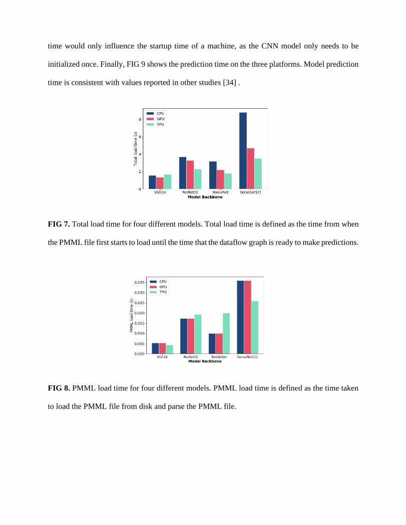
time would only influence the startup time of a machine, as the CNN model only needs to be

initialized once. Finally, FIG 9 shows the prediction time on the three platforms. Model prediction

time is consistent with values reported in other studies [34] .

FIG 7. Total load time for four different models. Total load time is defined as the time from when

the PMML file first starts to load until the time that the dataflow graph is ready to make predictions.

FIG 8. PMML load time for four different models. PMML load time is defined as the time taken

to load the PMML file from disk and parse the PMML file.

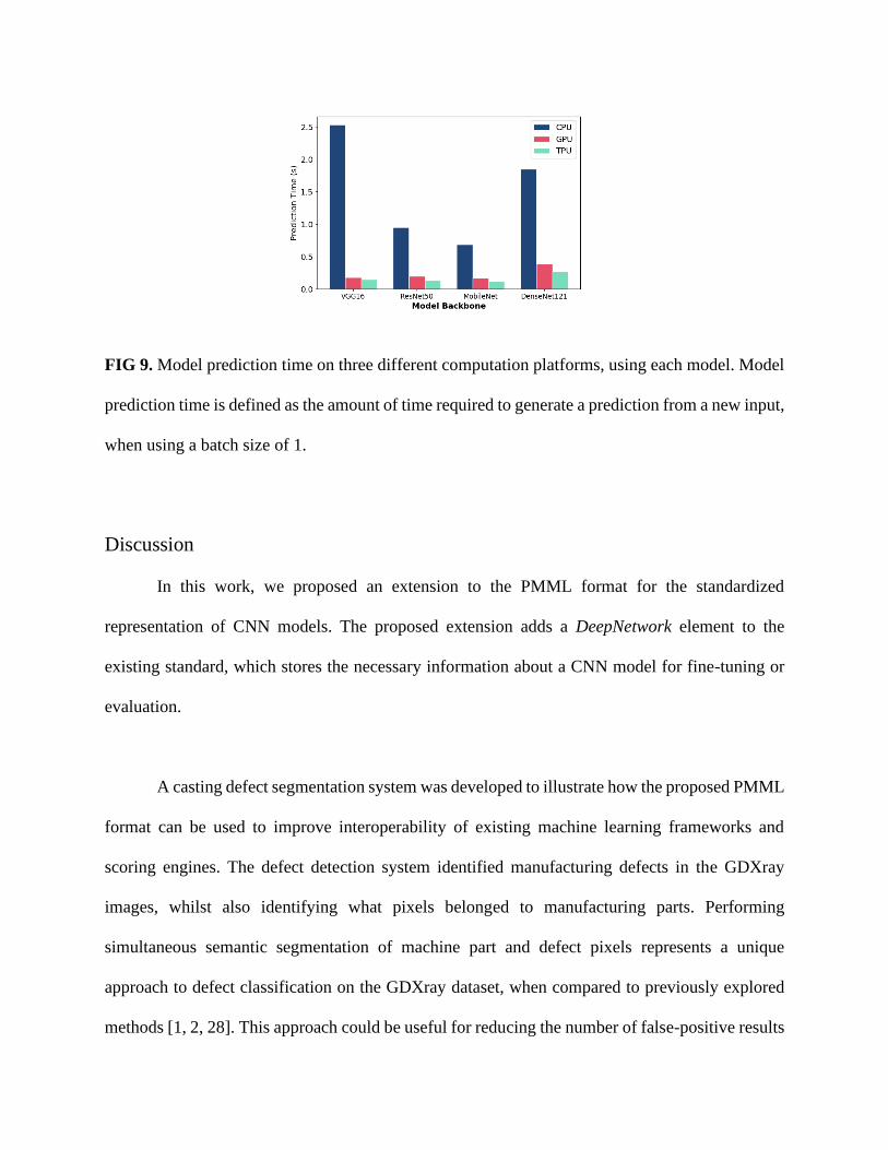
FIG 9. Model prediction time on three different computation platforms, using each model. Model

prediction time is defined as the amount of time required to generate a prediction from a new input,

when using a batch size of 1.

Discussion

In this work, we proposed an extension to the PMML format for the standardized

representation of CNN models. The proposed extension adds a DeepNetwork element to the

existing standard, which stores the necessary information about a CNN model for fine-tuning or

evaluation.

A casting defect segmentation system was developed to illustrate how the proposed PMML

format can be used to improve interoperability of existing machine learning frameworks and

scoring engines. The defect detection system identified manufacturing defects in the GDXray

images, whilst also identifying what pixels belonged to manufacturing parts. Performing

simultaneous semantic segmentation of machine part and defect pixels represents a unique

approach to defect classification on the GDXray dataset, when compared to previously explored

methods [1, 2, 28]. This approach could be useful for reducing the number of false-positive results

encountered when the defect detection system incorrectly finds defects outside the part, as

discussed in [1].

Historically, manufacturing researchers and technicians were concerned that deep learning

systems would require an infeasible amount of data to train. However, by leveraging transfer

learning, it is now possible to train a powerful computer vision system with as little as a thousand

training examples. In this work, the PMML CNN format is used as an intermediate representation

to store pretrained models before they are used to initialize the U-Net model weights. In this way,

PMML CNN reduced overall software complexity, as both the intermediate models and final

models were stored in the same format.

Purpose-built scoring engines will become increasingly important in the smart

manufacturing industry, especially as internet-connected manufacturing machines become more

mainstream. The response time and throughput capacity of these scoring engines are critical to the

adoption of predictive modeling in smart manufacturing. For many real-time applications, the

response time of the scoring machine must be sufficiently low to avoid manufacturing devices

becoming idle whilst waiting for feedback from the scoring engine. A high-performance scoring

engine was created using the proposed PMML format. Due to the declarative nature of the

proposed PMML format, it was possible for the scoring engine to evaluate models on CPU, GPU

or TPU hardware. This level of flexibility could be highly beneficial for manufacturing

applications, where models must be evaluated on embedded systems (CPU evaluation) or with

high-throughput and low latency (TPU evaluation).

Future work could focus on further extending the DeepNetwork element to support

complex CNN models, such as object detection or instance segmentation models. Another

opportunity for future work is to extend PMML to support more deep neural network types,

including Recurrent Neural Networks or Natural Language Models.

Conclusion

In this work, we proposed an extension to the PMML format for the standardized

representation of convolutional neural network models. A semantic segmentation-based casting

defect system was developed to illustrate how PMML CNN can improve the interoperability of

existing machine learning frameworks and scoring engines. Furthermore, a scoring engine was

created for this new standardized schema and used to evaluate the performance characteristics of

the proposed format. The scoring engine and the trained models have all been made publicly

available to accelerate research in the field.

ACKNOWLEDGMENTS

This research is partially supported by the Smart Manufacturing Systems Design and

Analysis Program at the National Institute of Standards and Technology (NIST), Grant Numbers

70NANB18H193 and 70NANB19H097 awarded to Stanford University.

DISCLAIMER

Certain commercial systems are identified in this paper. Such identification does not imply

recommendation or endorsement by NIST; nor does it imply that the products identified are

necessarily the best available for the purpose. Further, any opinions, findings, conclusions, or

recommendations expressed in this material are those of the authors and do not necessarily reflect

the views of NIST or any other supporting U.S. government or corporate organizations.

References

[1] M. Ferguson, R. Ak, Y.-T. T. Lee, and K. H. Law, “Detection and Segmentation of

Manufacturing Defects with Convolutional Neural Networks and Transfer Learning,” Smart

and Sustainable Manufacturing Systems (SSMS), vol. 2, no. 1, pp. 137–164, Oct. 2018,

https://doi.org/10.1520/SSMS20180033.

[2] M. Ferguson, R. Ak, Y.-T. T. Lee, and K. H. Law, “Automatic Localization of Casting Defects

with Convolutional Neural Networks,” International Conference on Big Data (IEEE Big

Data), Boston, USA, 2017, pp. 1726–1735, https://doi.org/10.1109/BigData.2017.8258115.

[3] P. Napoletano, F. Piccoli, and R. Schettini, “Anomaly Detection in Nanofibrous Materials by

CNN-Based Self-Similarity,” Sensors, vol. 18, no. 2, p. 209, 2018,

https://doi.org/10.3390/s18010209.

[4] Y. Chu, C. Huang, X. Xie, B. Tan, S. Kamal, and X. Xiong, “Multilayer Hybrid Deep-Learning

Method for Waste Classification and Recycling,” Computational Intelligence and

Neuroscience, vol. 1, pp. 1–9, 2018, https://doi.org/10.1155/2018/5060857.

[5] A. Memo et al., “Systems and Methods for Inspection and Defect Detection using 3D

Scanning,” US Patent Application US20180322623A1, filed April 08, 2017.

[6] L. K. Redden, J. P. Ostrowski, K. Anderson, and E. W. J. Pell, “Modular Precision Agriculture

System,” US Patent Application US20160255778A1, filed March 6, 2015.

[7] G. Pasqualotto et al., “System and Method for Portable Active 3D Scanning,” US Patent

US10204448B2, filed November 11, 2016. Issued February 12, 2019.

[8] M. Abadi et al., “TensorFlow: A System for Large-Scale Machine Learning,” Symposium on

Operating Systems Design and Implementation (OSDI), Savannah, GA, USA, 2016, vol. 16,

pp. 265–283.

[9] L. Roeder, “Netron,” A Viewer for Neural Network, Deep Learning and Machine Learning

Models., 2017. [Online]. Available: https://github.com/lutzroeder/netron. [Accessed: 17-Jul-

2019].

[10] S. Krishnan and J. L. U. Gonzalez, “Google Compute Engine,” Building Your Next Big Thing

with Google Cloud Platform, Springer, 2015, pp. 53–81.

[11] S. Ioffe and C. Szegedy, “Batch Normalization: Accelerating Deep Network Training by

Reducing Internal Covariate Shift,” International Conference on Machine Learning (ICML),

Lille, France, 2015.

[12] N. P. Jouppi et al., “In-Datacenter Performance Analysis of a Tensor Processing Unit,”

International Symposium on Computer Architecture (ISCA), Toronto, ON, Canada, 2017, pp.

1–12, https://doi.org/10.1145/3079856.3080246.

[13] S. J. Pan and Q. Yang, “A Survey on Transfer Learning,” IEEE Transactions on Knowledge

and Data Engineering (TKDE), vol. 22, no. 10, pp. 1345–1359, 2009,

https://doi.org/10.1186/s40537-016-0043-6.

[14] A. Guazzelli, M. Zeller, W. Lin, and G. Williams, “PMML: An Open Standard for Sharing

Models,” The R Journal, vol. 1, no. 1, pp. 60–65, 2009.

[15] D. Gorea, “Dynamically Integrating Knowledge in Applications. An Online Scoring Engine

Architecture,” International Conference on Development and Application Systems (DAS),

Suceava, Romania, 2008, vol. 3.

[16] I. Goodfellow, Y. Bengio, A. Courville, and Y. Bengio, Deep Learning, vol. 1. MIT press

Cambridge, 2016.

[17] J. Wu, Convolutional Neural Networks. [Online]. Available:

https://cs.nju.edu.cn/wujx/teaching/15_CNN.pdf [Accessed 08/08/2019]., 2017.

[18] J. Chaves, C. Curry, R. L. Grossman, D. Locke, and S. Vejcik, “Augustus: The Design and

Architecture of a PMML-based Scoring Engine,” International Conference on Knowledge

Discovery and Data Mining (KDD), Philadelphia, USA, 2006, pp. 38–46,

https://doi.org/10.1145/1289612.1289616.

[19] N. Ketkar, “Introduction to PyTorch,” Deep Learning with Python, Springer, 2017, pp. 195–

208.

[20] ONNX Project Contributors, “Open Neural Network Exchange (ONNX),” 11-Aug-2019.

[Online]. Available: https://onnx.ai/. [Accessed: 12-Aug-2019].

[21] K. He, X. Zhang, S. Ren, and J. Sun, “Deep Residual Learning for Image Recognition,” IEEE

Conference on Computer Vision and Pattern Recognition (CVPR), Las Vegas, NV, USA,

2016, pp. 770–778.

[22] R. L. Grossman, M. F. Hornick, and G. Meyer, “Data Mining Standards Initiatives,”

Communications of the ACM, vol. 45, no. 8, pp. 59–61, 2002.

[23] M. Ferguson et al., “A Standardized Representation of Convolutional Neural Networks for

Reliable Deployment of Machine Learning Models in the Manufacturing Industry,”

International Design Engineering Technical Conferences and Computers and Information in

Engineering Conference (IDETC/CIE 2019), Anaheim, CA, USA, 2019.

[24] J. Park et al., “Gaussian Process Regression (GPR) Representation Using Predictive Model

Markup Language (PMML),” Smart and Sustainable Manufacturing Systems, vol. 1, no. 1,

p. 121, 2017.

[25] M. Ferguson, “PMML Scoring Engine and Deep Neural Network Models,” 2019. [Online].

Available: https://github.com/maxkferg/python-pmml/. [Accessed: 12-Aug-2019].

[26] R. Ren, T. Hung, and K. C. Tan, “A Generic Deep-learning-based Approach for Automated

Surface Inspection,” IEEE Transactions on Cybernetics, vol. 48, no. 3, pp. 929–940, 2018,

https://doi.org/10.1109/TCYB.2017.2668395.

[27] D. Mery et al., “GDXray: The Database of X-ray Images for Nondestructive Testing,”

Journal of Nondestructive Evaluation, vol. 34, no. 4, p. 42, Nov. 2015,

https://doi.org/10.1007/s10921-015-0315-7.

[28] D. Mery and C. Arteta, “Automatic Defect Recognition in X-ray Testing using Computer

Vision,” IEEE Winter Conference on Applications of Computer Vision (WACV), Santa Rosa,

California, 2017, pp. 1026–1035.

[29] O. Ronneberger, P. Fischer, and T. Brox, “U-Net: Convolutional Networks for Biomedical

Image Segmentation,” International Conference on Medical Image Computing and

Computer-assisted Intervention (MICCAI), Munich, Germany, 2015, pp. 234–241.

[30] J. Ji, L. Wu, Z. Chen, J. Yu, P. Lin, and S. Cheng, “Automated Pixel-Level Surface Crack

Detection Using U-Net,” International Conference on Multi-disciplinary Trends in Artificial

Intelligence (MIWAI), Hanoi, Vietnam, 2018, pp. 69–78.

[31] P. Y. Simard, D. Steinkraus, J. C. Platt, and others, “Best Practices for Convolutional Neural

Networks Applied to Visual Document Analysis,” International Conference on Document

Analysis and Recognition (ICDAR), Edinburgh, UK, 2003, vol. 3, pp. 958–963.

[32] D. P. Kingma and J. Ba, “Adam: A Method for Stochastic Optimization,” presented at the

International Conference on Learning Representations (ICLR), San Diego, CA, USA, 2014.

[33] S. Behnel, M. Faassen, and I. Bicking, lxml: XML and HTML with Python. 2005.

[34] S. Bianco, R. Cadene, L. Celona, and P. Napoletano, “Benchmark Analysis of Representative

Deep Neural Network Architectures,” IEEE Access, vol. 6, pp. 64270–64277, 2018,

http://doi.org/10.1109/access.2018.2877890.

LIST OF FIGURE CAPTIONS

FIG 1. Dataflow graph for a small convolutional neural network. Neural network layers are

represented as nodes in the graph. Nodes shown in green (lighter) do not perform any mathematical

operations on the input tensor. Nodes shown in red have learnable parameters, whilst nodes shown

in blue (darker) do not have any learnable parameters.

FIG 2. The structure and contents of a DeepNetwork PMML file.

FIG 3. Two connected nodes in the neural network graph, represented using the DeepNetwork

PMML format.

FIG 4. Ten different neural network layers represented in the proposed DeepNetwork format.

Global Max Pooling is not included as it is very similar to the Max Pooling layer. Similarly,

Transposed Convolution is similar to the Convolution Layer and is not shown here.

FIG 5. Examples of different CNN output definitions using the PMML CNN extension.

FIG 6. Comparison of ground truth and predictions using the U-Net segmentation network with

DenseNet-121 Backbone.

FIG 7. Total load time for four different models. Total load time is defined as the time from when

the PMML file first starts to load until the time that the dataflow graph is ready to make predictions.

FIG 8. PMML load time for four different models. PMML load time is defined as the time taken

to load the PMML file from disk and parse the PMML file.

FIG 9. Model prediction time on three different computation platforms, using each model. Model

prediction time is defined as the amount of time required to generate a prediction from a new input,

when using a batch size of 1.