A Spiking Neuron Model of Serial-Order RecallFeng-Xuan Choo (fchoo@uwaterloo.ca)

Chris Eliasmith (celiasmith@uwaterloo.ca)Center for Theoretical Neuroscience, University of Waterloo

Waterloo, ON, Canada N2L 3G1

Abstract

Vector symbolic architectures (VSAs) have been used to modelthe human serial-order memory system for decades. Despitetheir success, however, none of these models have yet beenshown to work in a spiking neuron network. In an effort to takethe first step, we present a proof-of-concept VSA-based modelof serial-order memory implemented in a network of spikingneurons and demonstrate its ability to successfully encode anddecode item sequences. This model also provides some insightinto the differences between the cognitive processes of mem-ory encoding and subsequent recall, and establish a firm foun-dation on which more complex VSA-based models of memorycan be developed.Keywords: Serial-order memory; serial-order recall; vectorsymbolic architectures; holographic reduced representation;population coding; LIF neurons; neural engineering frame-work

IntroductionThe human memory system is able to perform a multitudeof tasks, one of which is the ability to remember and recallsequences of serially ordered items. In human serial recallexperiments, subjects are presented items at a fixed interval,typically in the range of two items per second up to one itemevery 4 seconds. After the entire sequence has been presentedthe subjects are then asked to recall the items presented tothem, either in order (serial recall), or in any order the sub-ject desires (free recall). Plotting the recall accuracy of thesubjects, experimenters often obtain a graph with a distinc-tive U-shape. This unique shape arises from what is knownas the primacy and recency effects. The primacy effect refersto the increase in recall accuracy the closer the item is to thestart of the sequence, and the recency effect refers to the sameincrease in recall accuracy as the item gets closer to the endof the sequence.

Many models have been proposed to explain this peculiarbehaviour in the recall accuracy data. Here we will concen-trate on one class of models which employ vector symbolicarchitectures (VSAs) to perform the serial memory and re-call. Using VSAs to perform serial memory tasks would beinsufficient however, if the VSA-based model cannot be im-plemented in spiking neurons, and thus, cannot be used toexplain what the brain is actually doing. In this paper, wethus present a proof-of-concept VSA-based model of serialrecall implemented using spiking neurons.

Vector Symbolic ArchitectureThere are four core features of vector symbolic architectures.First, information is represented by randomly chosen vectorsthat are combined in a symbol-like manner. Second, a super-position operation (here denoted with a +) is used to combine

vectors such that the result is another vector that is similar tothe original input vectors. Third, a binding operation (⊗) isused to combine vectors such that the result is a vector thatis dissimilar to original vectors. Last, an approximate inverseoperation (denoted with ∗, such that A∗ is the approximate in-verse of A) is needed so that previously bound vectors can beunbound.

A⊗B⊗B∗ ≈ A (1)

Just like addition and multiplication, the VSA operations areassociative, commutative, and distributive.

The class of VSA used in this model is the HolographicReduced Representation (HRR) (Plate, 2003). In this repre-sentation, each element of an HRR vector is chosen from anormal distribution with a mean of 0, and a variance of 1/nwhere n is the number of elements there are in the vector. Thestandard addition operator is used to perform the superposi-tion operation, and the circular convolution operation is usedto perform the binding operation. The circular convolution oftwo vectors can be efficiently computed by utilizing the FastFourier Transform (FFT) algorithm:

x⊗y = F −1(F (x)�F (y)), (2)

where F and F −1 are the FFT and inverse FFT operationsrespectively, and � is the element-wise multiplication of thetwo vectors. The circular convolution operation, unlike thestandard convolution operation, does not change the dimen-sionality of the result vector. This makes the HRR extremelysuitable for a neural implementation because it means that thedimensionality of the network remains constant regardless ofthe number of operations performed.

The VSA-based Approach to Serial MemoryThere are multiple ways in which VSAs can be used toencode serially ordered items into a memory trace. TheCADAM model (Liepa, 1977) provides a simple example ofhow a sequence of items can be encoded as a single mem-ory trace. In the CADAM model, the sequence containingthe items A, B, and C would be encoded as in single memorytrace, MABC as follows:

MA = AMAB = A+A⊗B

MABC = A+A⊗B+A⊗B⊗C

The model presented in this paper, however, takes inspira-tion from behavioural data obtained from macaque monkeys.This data suggests that each sequence item is encoded using

2188

ordinal information (Orlov, Yakovlev, Hochstein, & Zohary,2000), rather than being “chained” together as in the CADAMmodel. To achieve this, additional vectors are used to repre-sent the ordinal information of each item. In the subsequentequations, this ordinal vector is represented as Pi, where iindicates the item’s ordinal number in each sequence. Thememory trace MABC would thus be computed like so:

MA = P1⊗A (3)MAB = P1⊗A+P2⊗B (4)

MABC = P1⊗A+P2⊗B+P3⊗B (5)

The encoding strategy presented above does not seem tohave any mechanism by which to explain the primacy or re-cency effects seen in human behavioural data. In order toachieve these effects, additional components are added to themodel. These components are discussed further below.

Neural RepresentationTo implement any of these models, we need to determine howa vector can be represented by a population of spiking neu-rons. In 1986, Georgopoulos et al. demonstrated that in thebrain, 2D movement directions are encoded by a large pop-ulation of neurons, with each neuron being most active forone specific direction – their preferred direction. The activityof each neuron would then indicate the similarity of the in-put vector to each neuron’s preferred direction vector. Sincethe movement direction is essentially a two-dimensional vec-tor, this method of vector representation can be extended tomultiple dimensions as well. For a population of neurons, thecurrent J flowing into neuron i can then be calculated by thefollowing equation.

Ji(x) = αi(φ̃i ·xi)+ Jbiasi (6)

In the above equation, the dot product computes the similaritybetween the input vector x and the neuron’s preferred direc-tion vector φ̃. The neuron gain is denoted by α, while Jbias

denotes a fixed background input current. The current Ji canthen be used as the input to any neuron model G[·] to ob-tain the activity for neuron i. In this model, we use the leakyintegrate-and-fire (LIF) neuron model, characterized as such:

ai(x) = Gi[Ji(x)] =1

τre f − τRC ln(

1− Jth

Ji(x)

) , (7)

where ai(x) is the average firing rate of the neuron i, τre f

is the neuron refractory time constant, τRC is the neuron RCtime constant, and Jth is the neuron threshold firing current.For a time-varying input x(t), the equations remain the same,with the exception that the activity of the neuron is no longeran average firing rate, but rather a spike train:

a(x(t)) = ∑n

δ(t− tn) (8)

Since the spike train represents the neuron’s response to theinput vector x, given the spike trains from all the neurons in

the population, it should be possible to derive decoding vec-tors φ that can be used to estimate the original input. Elia-smith and Anderson (2003) demonstrate that these decodingvectors can be found using the following equation.

φ = Γ−1

ϒ, where

Γi j =Z

ai(x)a j(x) dx ϒi =Z

ai(x)x dx(9)

By weighting the decoding vectors with the post-synaptic cur-rent h(t) generated by each spike, it is then possible to con-struct x̂(t), an estimate of the input vector. Equation (10)demonstrates how this is achieved. The parameters used togenerate the shape of h(t) is determined by the neurophysiol-ogy of the neuron population.

x̂(t) = ∑i,n

δ(t− tin)∗h(t)φi

= ∑i,n

h(t− tin)φi (10)

The encoding and decoding vectors also provides a methodby which the optimal connection weights between two neu-ral populations can be. If for example, the transformationbetween two populations of neurons is a simple scaling oper-ation, where the output of the second group of neurons shouldbe Cx, then the connection weights w between the populationsshould be

wi j = Cα jφ̃ jφi (11)

Extending Equation (7) for linear operations is also straight-forward. Consider three neural populations: one to representthe input x, another to represent the input y, and a third that wewish to have compute the linear combination Cx + Dy. Theactivity of the neurons in final population can be determinedby

ck(Cx+Dy) = Gk

[∑

iwkiai(x)+∑

jwk jb j(y)+ Jbias

k

], (12)

where ai, b j, and ck are the activities of the neurons in thefirst, second and third neural populations respectively. Em-ploying Equation (11), the synaptic connection weights canalso be determined. Letting wki be the connection weightsbetween the first and third population, and wk j be the connec-tion weights between the second and third population, theywork out to be:

wki = αkφ̃kφxi and wk j = αkφ̃kφ

yj (13)

Note that in the equation above, the superscripts serves todisambiguate the decoders, where φx signifies the decodersthat represent x, and likewise for φy. Eliasmith and Anderson(2003) go into greater detail on how to use this general frame-work, known as the Neural Engineering Framework, to derivethe appropriate decoders and connection weights to performarbitrary non-linear operations as well.

2189

The Neural ModelThe neural model implemented in this paper is divided intotwo neural processes. One encodes an item sequence into asingle memory trace, and the other decodes an encoded mem-ory trace to retrieve its constituent items.

Sequence EncoderAnalysis of Equations (3) to (5) show that the memory tracefor an arbitrary sequence of items can be constructed by com-puting the convolution of the last item vector with its ordinalvector, and then adding the result of the convolution to thememory trace of the sequence less the final item. From this,a generic sequence encoding equation can be derived (fromhere on referred to as the basic encoding equation).

Mi = Mi−1 +Pi⊗ Ii (14)

In the equation above, Mi represents the memory trace afterencoding the ith item. Pi and Ii represents the ith item’s ordinalvector and item vector respectively.

As mentioned previously, the encoding equation in its ba-sic form does not account for the primacy and recency effectsseen in human behavioural data. To achieve the primacy ef-fect, rehearsal is simulated by adding an additional weightedcopy of the old memory trace to the memory trace being cal-culated for the current item. In essence, as each item is re-hearsed, a weighted copy of the item is added to the memorytrace to “boost” the item’s representation within the mem-ory trace. In the equation below, the memory trace of therehearsal-based encoding is denoted by Ri and the weight ap-plied to the rehearsed contribution of the old memory traceis denoted by α. In the model implemented for this paper, α

was set to 0.3.

Ri = Ri−1 +Pi⊗ Ii +αRi−1 (15)= (1+α)Ri−1 +Pi⊗ Ii (16)

To achieve the recency effect, an separate memory compo-nent is added to play the role of a sensory input buffer. Theinput buffer encodes items in a similar fashion to Equation(14) with a decay added to the old memory trace. This decaycauses the input buffer to store only the most recently pre-sented items, thus mimicking the basic recall characteristicsof the human working memory system. In the neural imple-mentation of this model, the decay is achieved by tuning theintegrators used in the memory modules to slowly drift to zeroif no additional input is applied to them. Equation (17) illus-trates how this decay can be represented mathematically, withthe memory trace of the input buffer represented by Bi, andthe rate of decay represented by β.

Bi = βBi−1 +Pi⊗ Ii (17)

The final memory trace of the encoded item sequence isthen computed by combining the memory trace from therehearsal component and the memory trace from the inputbuffer component.

Mi = Ri +Bi (18)

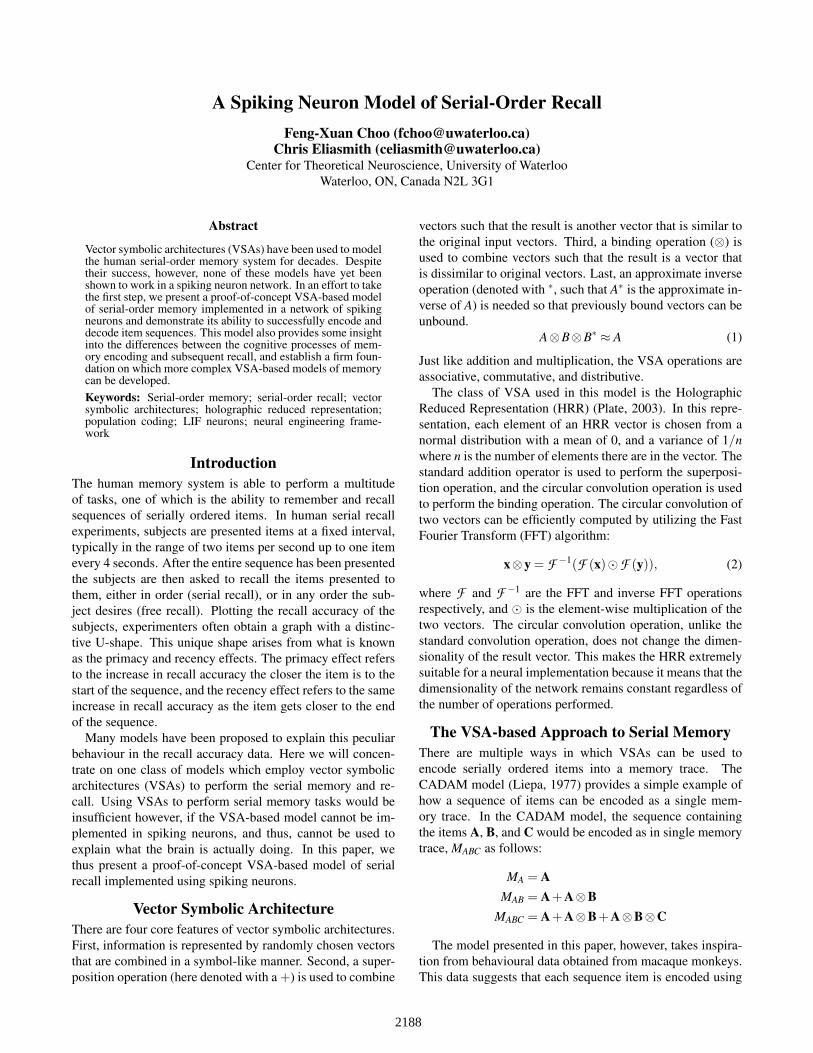
From the above encoding equations, several issues becomeevident. First, two operations need to be implemented – a cir-cular convolution and an addition operation. Second, a mem-ory module is needed to hold the value of Mi−1 while the newmemory trace Mi is computed. With these components, andthe rehearsal and decay mechanisms described above, a highlevel block diagram of the complete encoding network can beconstructed, as shown in Figure 1.

Encoded

Sequence

Vector

Ii

Ri-1 Bi-1

Mi

Memory Module

(with decay)

Memory

Module

+

Pi

+

+

Ri Bi

Rehearsal

Component

Input Buffer

Component

Figure 1: Encoding network functional block diagram.

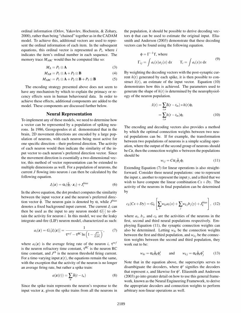
Sequence DecoderThe decoding process is much simpler than the encoding pro-cess. The first step of the decoding process is to convolvethe encoded memory trace with the inverse of the desired or-dinal vector. For example, if the system is trying to decodethe second item in the sequence, the encoded memory tracewould be convolved with the inverse of P2. Next, the resultof this convolution is fed to a cleanup memory module. Thecleanup memory module contains a copy of all the item vec-tors in the original sequence, and when given an input, willdetermine which of the original item vectors best matches theinput vector. An example of this decoding process follows.To simplify the example, only the basic encoding equation isused.

MABC = P1⊗A+P2⊗B+P3⊗BCB = MABC⊗P∗2

= P1⊗A⊗P∗2 +P2⊗B⊗P∗2 +P3⊗B⊗P∗2≈ P1⊗A⊗P∗2 +B+P3⊗B⊗P∗2

IB = cleanup(CB)≈ B

From the example above, we see that convolving the mem-ory trace MABC with the inverse of P2 results in a vector withthe desired item vector B combined with the unwanted vec-tors (P1 ⊗A⊗ P∗2 ) and (P3 ⊗B⊗ P∗2 ). However, since thecleanup memory module only contains the item vectors from

2190

the original sequence and not the superfluous vectors, feedingthe result of the convolution through the cleanup memory iso-lates the item vector B, producing the desired result. Figure 2illustrates the high level block diagram used to implement thedecoding network.

Cleanup

Memory Pi

Menc Recalled

Item

Vector (*)

Figure 2: Decoding network functional block diagram.

Performing the Binding Operation Referring back toEquation (2) we see that the binding operation can be cal-culated using the FFT and IFFT algorithms, so the first stepto implementing the binding operation in neurons is to imple-ment these two operations. The equations that compute theFFT and IFFT algorithms are as follows:

FFT : Xk =N−1

∑n=0

xne−2πiN kn k = 0, ...,N−1

IFFT : xn =1N

N−1

∑k=0

Xke2πiN kn n = 0, ...,N−1

(19)

Taking a closer look at the equations above, we see that theycan be implemented efficiently as a multiplication betweenthe input vector and a matrix containing the FFT (or IFFT)coefficients. From Equation (11), we can then set the synap-tic connection weight matrix as the Fourier transform coef-ficients to calculate the required FFT and IFFT operations.The one caveat to this approach is that the real and imagi-nary components of the Fourier transform have to calculatedseparately and then recombined (with the appropriate signchanges) when the final result is calculated.

With the neural implementation of the Fourier transformssolved, the implementation of the circular convolution bind-ing operation becomes trivial since the only other opera-tion needed is an element-wise multiplication. This can beachieved by utilizing multiple neural populations, each han-dling one element in the element-wise multiplication.

The Memory Module Since the circular convolution andaddition operations are essentially feed-forward neural net-works, the memory module in this model needs to be ableto drive the network with a constant value and store the newvalue at the same time. This is achieved by the use of gatedintegrators. When the integrator is not being gated, it attemptsto match the value of the input signal. When the integrator isgated, it no longer responds to the input value, and outputsthe previously stored value. By placing two gated integratorsin parallel controlled by complementary gating signals, thememory module is able to simultaneously store the new inputvalue while outputting the previously stored value.

Cleanup Memory The cleanup memory network used inthis model is an extension of the cleanup memory presentedin (Stewart, Tang, & Eliasmith, 2009). In essence, the im-plementation of cleanup memory involves creating multipleneural populations, each assigned to one item vector from theoriginal item sequence. The preferred direction vectors φ̃ foreach neuron in one population is predefined to match the itemvector it is meant to clean up. From Equation (6), we see thatthe the similarity (dot product) is calculated to determine theactivity of the neuron. By predefining φ̃, we can then deter-mine the similarity of the decoded item vector to each of theoriginal item vectors, thus determining which of the originalitem vectors best matches the decoded item vector.

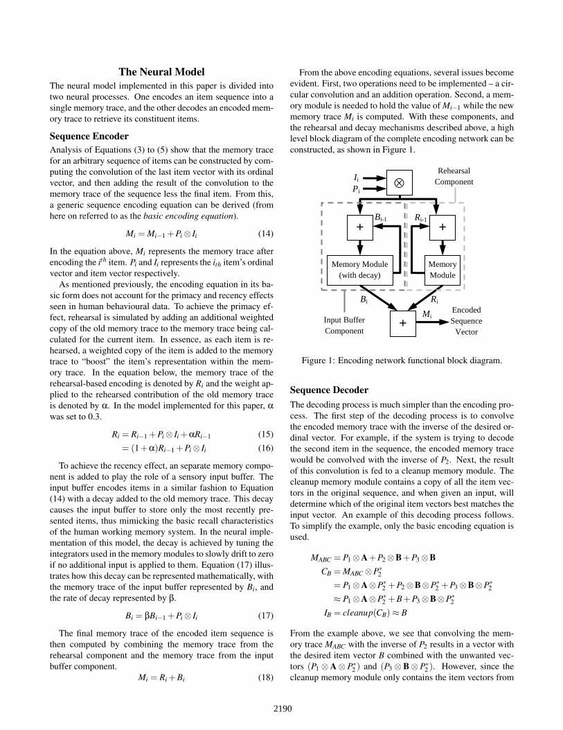
Combining the Encoder and DecoderGetting the spiking neuron model to encode a sequence, andsubsequently decode the memory trace is achieved by chain-ing the encoder and the decoder together. Control signals areused to ensure that the decoding network only commences af-ter the encoder has finished encoding the last item vector. Fig-ure 3 shows the results of the complete network encoding anddecoding a example twenty-dimensional 4-itemed sequence.

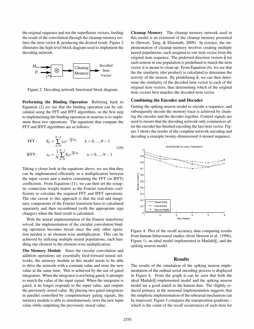
Figure 4: Plot of the recall accuracy data comparing resultsfrom human behavioural studies (from Henson et al. (1996),Figure 1), an ideal model implemented in Matlab R©, and thespiking neuron model.

ResultsThe results of the simulation of the spiking neuron imple-mentation of the ordinal serial encoding process is displayedin Figure 4. From the graph it can be seen that both theideal Matlab R©-implemented model and the spiking neuronmodel are a good match to the human data. The slightly re-duced primacy in the neuronal implementation suggests thatthe simplistic implementation of the rehearsal mechanism canbe improved. Figure 5 compares the transposition gradients –which is the count of the recall occurrences of each item for

2191

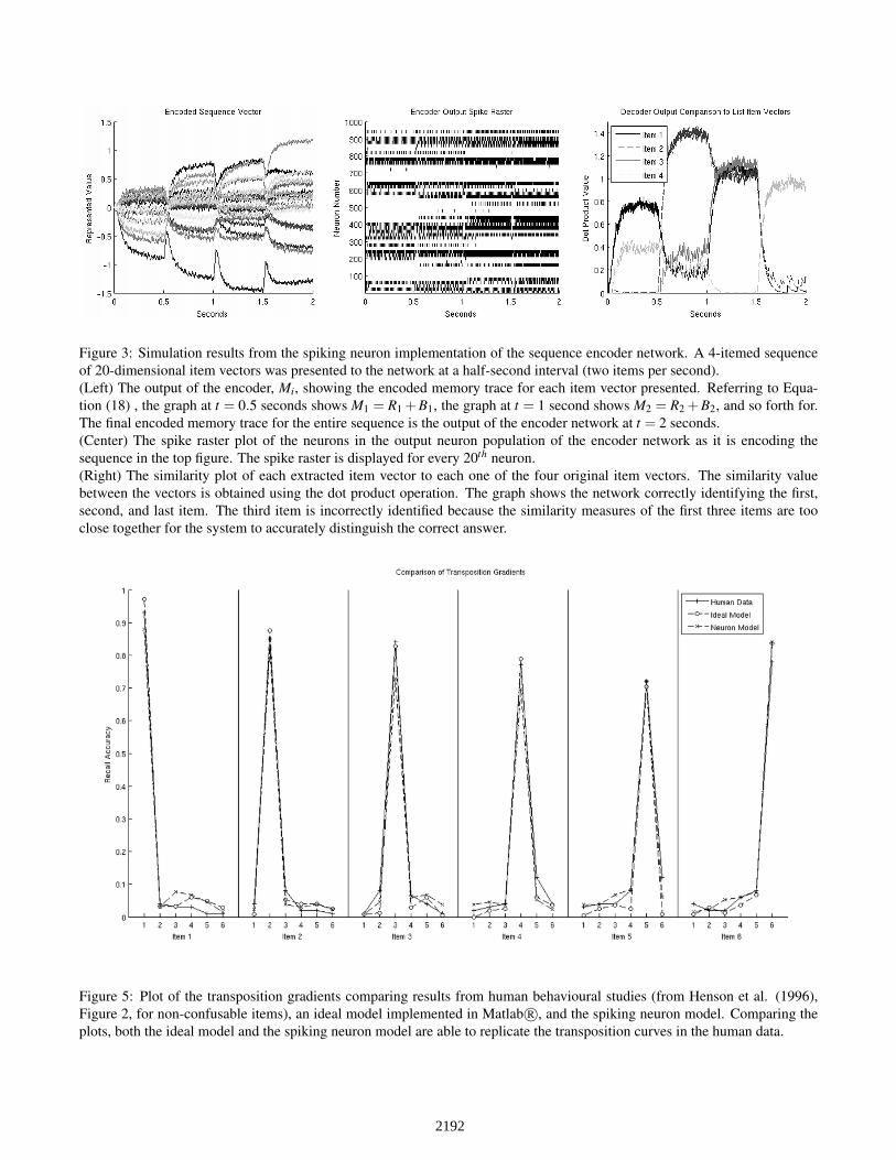
Figure 3: Simulation results from the spiking neuron implementation of the sequence encoder network. A 4-itemed sequenceof 20-dimensional item vectors was presented to the network at a half-second interval (two items per second).(Left) The output of the encoder, Mi, showing the encoded memory trace for each item vector presented. Referring to Equa-tion (18) , the graph at t = 0.5 seconds shows M1 = R1 + B1, the graph at t = 1 second shows M2 = R2 + B2, and so forth for.The final encoded memory trace for the entire sequence is the output of the encoder network at t = 2 seconds.(Center) The spike raster plot of the neurons in the output neuron population of the encoder network as it is encoding thesequence in the top figure. The spike raster is displayed for every 20th neuron.(Right) The similarity plot of each extracted item vector to each one of the four original item vectors. The similarity valuebetween the vectors is obtained using the dot product operation. The graph shows the network correctly identifying the first,second, and last item. The third item is incorrectly identified because the similarity measures of the first three items are tooclose together for the system to accurately distinguish the correct answer.

Figure 5: Plot of the transposition gradients comparing results from human behavioural studies (from Henson et al. (1996),Figure 2, for non-confusable items), an ideal model implemented in Matlab R©, and the spiking neuron model. Comparing theplots, both the ideal model and the spiking neuron model are able to replicate the transposition curves in the human data.

2192

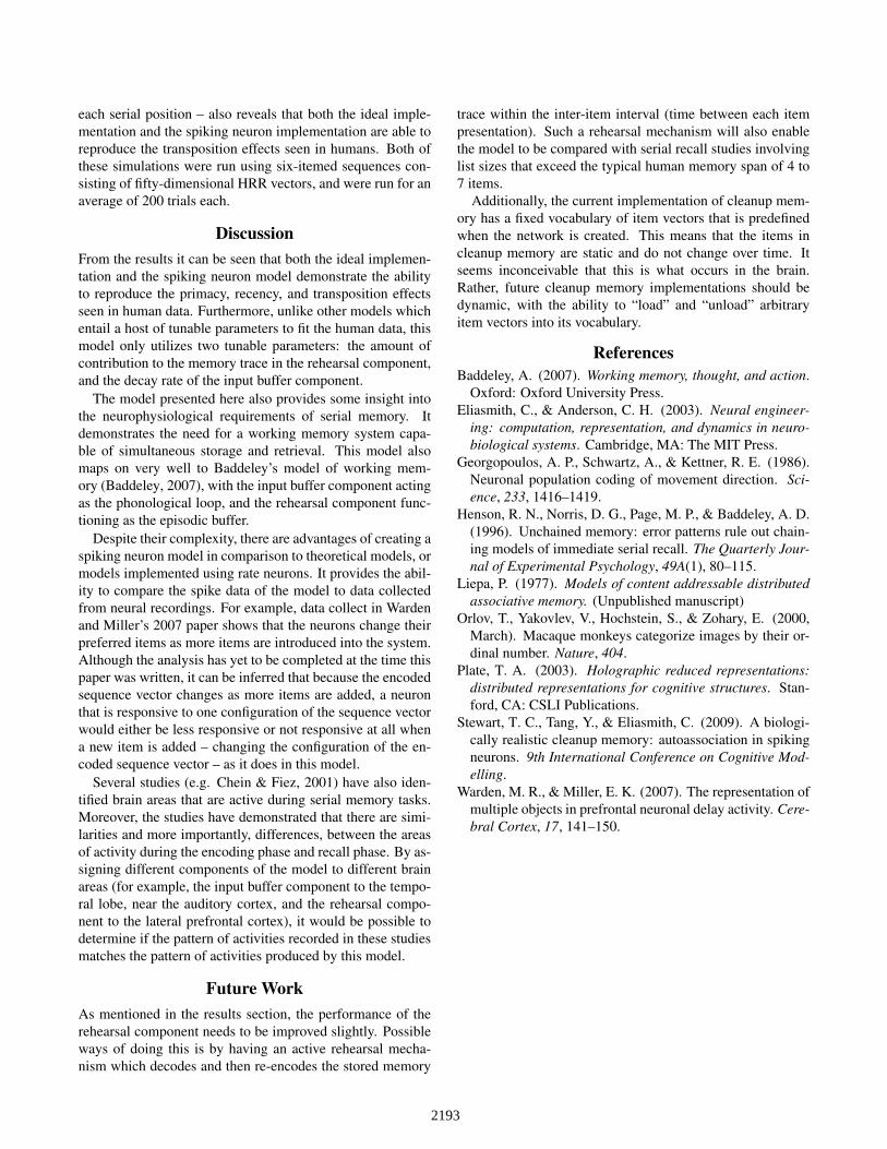
each serial position – also reveals that both the ideal imple-mentation and the spiking neuron implementation are able toreproduce the transposition effects seen in humans. Both ofthese simulations were run using six-itemed sequences con-sisting of fifty-dimensional HRR vectors, and were run for anaverage of 200 trials each.

DiscussionFrom the results it can be seen that both the ideal implemen-tation and the spiking neuron model demonstrate the abilityto reproduce the primacy, recency, and transposition effectsseen in human data. Furthermore, unlike other models whichentail a host of tunable parameters to fit the human data, thismodel only utilizes two tunable parameters: the amount ofcontribution to the memory trace in the rehearsal component,and the decay rate of the input buffer component.

The model presented here also provides some insight intothe neurophysiological requirements of serial memory. Itdemonstrates the need for a working memory system capa-ble of simultaneous storage and retrieval. This model alsomaps on very well to Baddeley’s model of working mem-ory (Baddeley, 2007), with the input buffer component actingas the phonological loop, and the rehearsal component func-tioning as the episodic buffer.

Despite their complexity, there are advantages of creating aspiking neuron model in comparison to theoretical models, ormodels implemented using rate neurons. It provides the abil-ity to compare the spike data of the model to data collectedfrom neural recordings. For example, data collect in Wardenand Miller’s 2007 paper shows that the neurons change theirpreferred items as more items are introduced into the system.Although the analysis has yet to be completed at the time thispaper was written, it can be inferred that because the encodedsequence vector changes as more items are added, a neuronthat is responsive to one configuration of the sequence vectorwould either be less responsive or not responsive at all whena new item is added – changing the configuration of the en-coded sequence vector – as it does in this model.

Several studies (e.g. Chein & Fiez, 2001) have also iden-tified brain areas that are active during serial memory tasks.Moreover, the studies have demonstrated that there are simi-larities and more importantly, differences, between the areasof activity during the encoding phase and recall phase. By as-signing different components of the model to different brainareas (for example, the input buffer component to the tempo-ral lobe, near the auditory cortex, and the rehearsal compo-nent to the lateral prefrontal cortex), it would be possible todetermine if the pattern of activities recorded in these studiesmatches the pattern of activities produced by this model.

Future WorkAs mentioned in the results section, the performance of therehearsal component needs to be improved slightly. Possibleways of doing this is by having an active rehearsal mecha-nism which decodes and then re-encodes the stored memory

trace within the inter-item interval (time between each itempresentation). Such a rehearsal mechanism will also enablethe model to be compared with serial recall studies involvinglist sizes that exceed the typical human memory span of 4 to7 items.

Additionally, the current implementation of cleanup mem-ory has a fixed vocabulary of item vectors that is predefinedwhen the network is created. This means that the items incleanup memory are static and do not change over time. Itseems inconceivable that this is what occurs in the brain.Rather, future cleanup memory implementations should bedynamic, with the ability to “load” and “unload” arbitraryitem vectors into its vocabulary.

ReferencesBaddeley, A. (2007). Working memory, thought, and action.

Oxford: Oxford University Press.Eliasmith, C., & Anderson, C. H. (2003). Neural engineer-

ing: computation, representation, and dynamics in neuro-biological systems. Cambridge, MA: The MIT Press.

Georgopoulos, A. P., Schwartz, A., & Kettner, R. E. (1986).Neuronal population coding of movement direction. Sci-ence, 233, 1416–1419.

Henson, R. N., Norris, D. G., Page, M. P., & Baddeley, A. D.(1996). Unchained memory: error patterns rule out chain-ing models of immediate serial recall. The Quarterly Jour-nal of Experimental Psychology, 49A(1), 80–115.

Liepa, P. (1977). Models of content addressable distributedassociative memory. (Unpublished manuscript)

Orlov, T., Yakovlev, V., Hochstein, S., & Zohary, E. (2000,March). Macaque monkeys categorize images by their or-dinal number. Nature, 404.

Plate, T. A. (2003). Holographic reduced representations:distributed representations for cognitive structures. Stan-ford, CA: CSLI Publications.

Stewart, T. C., Tang, Y., & Eliasmith, C. (2009). A biologi-cally realistic cleanup memory: autoassociation in spikingneurons. 9th International Conference on Cognitive Mod-elling.

Warden, M. R., & Miller, E. K. (2007). The representation ofmultiple objects in prefrontal neuronal delay activity. Cere-bral Cortex, 17, 141–150.

2193