Embed Size (px)
Citation preview
Department of Mechanical Engineering
A Specification for Measuring Domestic Energy Demand
Profiles
Author: Katalin M Svehla
Supervisor: Professor Joe Clarke
A thesis submitted in partial fulfilment for the requirement of degree in
Master of Science in Renewable Energy Systems and the Environment
2011
A Specification for Measuring Domestic Energy Demand Profiles
Page 2 of 120
Copyright Declaration
This thesis is the result of the author‟s original research. It has been composed by the author
and has not been previously submitted for examination which has led to the award of a
degree.
The copyright of this thesis belongs to the author under the terms of the United Kingdom
Copyright Acts as qualified by University of Strathclyde Regulation 3.50. Due
acknowledgement must always be made of the use of any material contained in, or derived
from, this thesis.
Signed: Date: 7 September 2011
Page 3 of 120
Abstract
Demand profiles, which show how energy use varies over time, are being increasingly used to
look at the impacts of changes in energy supply and use. Applications range from investigating
how well intermittent, renewable energy sources can fulfil demand, to evaluating the impacts on
distribution networks and to underpinning strategic decisions about future energy scenarios.
Domestic energy demand fluctuates by the minute and exhibits daily, weekly and seasonal
patterns; however, the only data that are available widely are aggregated and averaged national
statistics, so researchers tend to make their own measurements when they need demand profiles.
These measurements are necessarily limited in the number and types of households, the range of
energy use they cover, and in duration. On the other hand, those measurement programmes that
have covered a wider scope have found that apparently similar households can have very
different consumption patterns due to differing habits and attitudes. It is difficult to compare
results between studies because they typically measure different things, and most cases the
source data are not published for commercial or data privacy reasons.
If future studies were to follow a common standard for measuring domestic load profiles and
pool the source data in a suitably non-personalised way, this could eventually yield better
insights into what drives energy use and how it varies by geography and over time; in the worst
case, higher quality statistical data would be available. A set of requirements for a standard,
comprehensive methodology for collecting demand profile is derived from a systematic review
of the literature as well as further analysis on one good-quality data set that has been made
publicly available. A specification is proposed for the measurements, in which demand is
collected by end use as well as by fuel type, prioritising the biggest energy users and those which
have the potential for demand shifting or fuel substitution – heating, hot water, cooking,
washing. Measurement is at the highest level of resolution needed to give a clear picture of
events and peak loads – 1 minute for electricity and 5 minutes for gas. Around 40 sets of data
are collected per house, together with a survey of the house and household context. Compared to
recent large-scale monitoring programmes in New Zealand and parts of the European Union, this
approach would yield less information on individual appliances, but would give high-resolution,
yearly profiles on all fuels used domestically, and on all major end-uses apart from transport.
Observations were made on the energy use in one household to look how the measurement plan
would be implemented in practice: these indicate that the significant end-use categories would be
covered between 80-100%.

A Specification for Measuring Domestic Energy Demand Profiles
Page 4 of 120
Acknowledgements
I would like to thank the following people who helped me complete this project:
My supervisor, Prof Joe Clarke, for guidance, support, challenges to lazy thinking, and most
especially for suggesting a topic that turned out more interesting than I had thought.
Kevin Spencer of Elexon for providing additional information and answering questions about
collecting and analysing load data.
Ian Richardson of Loughborough University for making his data available in the first place, and
for discussions about practical issues he encountered.
My neighbour, Adam Clark, who was willing to share information about his household energy
use and who let me play with his newly installed smart meter.
My husband Gerry Byrne, who supported me throughout and whose devotion to improving the
energy performance of the various houses we have lived in over the years was the reason for my
becoming interested in the subject in the first place.
A Specification for Measuring Domestic Energy Demand Profiles
Page 5 of 120
Contents
Copyright Declaration .............................................................................................................. 2
Abstract .................................................................................................................................... 3
Acknowledgements .................................................................................................................. 4
1. Introduction ............................................................................................................................ 12
1.1 Objectives ....................................................................................................................... 13
2 Literature review .................................................................................................................... 15
2.1 Operational support ........................................................................................................ 15
2.1.1 Scheduling and despatch ......................................................................................... 15
2.1.2 Settlements .............................................................................................................. 17
2.1.3 Managing energy use .............................................................................................. 18
2.2 Developing and validating energy demand models ........................................................ 18
2.2.1 Household energy consumption models ................................................................. 18
2.2.2 Energy demand simulation ...................................................................................... 21
2.3 Inputs for other modelling .............................................................................................. 24
2.3.1 Supply-demand balance with renewable and distributed generation ...................... 24
2.3.2 Behaviour of electricity distribution networks ........................................................ 28
2.3.3 Decision support for policy changes ....................................................................... 30
2.4 Demand profile measurements ....................................................................................... 31
2.4.1 UK studies ............................................................................................................... 32
2.4.2 Outside the UK ........................................................................................................ 38
2.5 Influence of social attitudes and habits........................................................................... 42
3 Lessons from demand profiling ............................................................................................. 46
3.1 Data availability .............................................................................................................. 46
3.2 Fuel inputs versus energy end use .................................................................................. 47
A Specification for Measuring Domestic Energy Demand Profiles
Page 6 of 120
3.3 What the sample represents ............................................................................................ 48
3.3.1 Size and composition .............................................................................................. 48
3.3.2 Energy consumption ................................................................................................ 49
3.3.3 Other context ........................................................................................................... 50
3.4 Data collection ................................................................................................................ 50
3.4.1 Frequency ................................................................................................................ 50
3.4.2 Duration ................................................................................................................... 51
3.4.3 Immediacy ............................................................................................................... 51
3.4.4 Consistency and accuracy ....................................................................................... 52
3.5 Practical issues ................................................................................................................ 53
3.5.1 Finding volunteers ................................................................................................... 53
3.5.2 Data privacy ............................................................................................................ 53
3.5.3 Access and equipment location ............................................................................... 53
3.5.4 Data transmission and storage ................................................................................. 53
3.5.5 Cost and effort considerations ................................................................................. 54
3.6 Consistency in outcomes ................................................................................................ 54
3.6.1 Energy use ............................................................................................................... 54
3.6.2 Correlations ............................................................................................................. 55
3.6.3 Attitudes and behaviours ......................................................................................... 56
4 Analysis of a high quality data set ......................................................................................... 57
4.1 Background ..................................................................................................................... 57
4.2 Accuracy, immediacy and quality of the data ................................................................ 57
4.3 Data processing approach ............................................................................................... 59
4.4 Comparison with population .......................................................................................... 60
4.5 Further analyses .............................................................................................................. 62
4.5.1 Energy use ............................................................................................................... 62
A Specification for Measuring Domestic Energy Demand Profiles
Page 7 of 120
4.5.2 Individual houses and appliance use ....................................................................... 62
4.5.3 Groups of dwellings ................................................................................................ 67
4.5.4 Effect of measurement resolution ........................................................................... 69
4.5.5 Evidence of trends ................................................................................................... 69
4.6 Conclusions from data analysis ...................................................................................... 73
5 Specification for a standard, comprehensive data set ............................................................ 74
5.1 Measurement plan requirements ..................................................................................... 74
5.2 Data ................................................................................................................................. 75
5.2.1 Fuel use and general context ................................................................................... 75
5.2.2 Space Heating .......................................................................................................... 76
5.2.3 Hot Water ................................................................................................................ 77
5.2.4 Cooking ................................................................................................................... 78
5.2.5 Lighting ................................................................................................................... 79
5.2.6 Cold Appliances ...................................................................................................... 80
5.2.7 Wet appliances ........................................................................................................ 80
5.2.8 Consumer electronics .............................................................................................. 81
5.2.9 Computers and other miscellaneous appliances ...................................................... 82
5.3 Frequency and duration of measurements ...................................................................... 82
5.4 How typical is the sample ............................................................................................... 83
5.5 Data capture and storage ................................................................................................. 83
5.6 Data collection process ................................................................................................... 84
5.6.1 Starting out .............................................................................................................. 84
5.6.2 Running and completing the data collection ........................................................... 86
5.7 Comparison with methodology used elsewhere ............................................................. 87
6 Observations of energy use in one house ............................................................................... 88
6.1 Description...................................................................................................................... 88
A Specification for Measuring Domestic Energy Demand Profiles
Page 8 of 120
6.1.1 House and occupancy .............................................................................................. 88
6.1.2 Instrumentation ........................................................................................................ 88
6.1.3 Observation method ................................................................................................ 89
6.2 Observations on energy use ............................................................................................ 89
6.2.1 Electrical appliances and overall electricity use ..................................................... 89
6.2.2 Gas consumption and secondary heating ................................................................ 92
6.3 The plan as applied to the observation house ................................................................. 94
6.4 Lessons for planning data collection .............................................................................. 94
7 Conclusions ............................................................................................................................ 96
7.1 Recommendations for further work ................................................................................ 97
References ..................................................................................................................................... 98
Appendix 1: Regional variations in domestic energy use - 2008 ................................................ 103
Appendix 2: Summary of data sets reviewed .............................................................................. 105
Appendix 3: Data collection plan ................................................................................................ 110
Appendix 4: Loughborough 1-minute resolution electricity demand data ................................ 116
A Specification for Measuring Domestic Energy Demand Profiles
Page 9 of 120
List of figures
Figure 1-1 UK energy end use 2008 ............................................................................................ 12
Figure 2-1 UK electricity system forecast and actual daily profiles ............................................. 16
Figure 2-2 Domestic electricity profiles for a winter weekday .................................................... 17
Figure 2-3 Annual variation in lighting demand for one half-hour in the day ............................. 19
Figure 2-4 Example simulation of electrical demand profile on one day ..................................... 22
Figure 2-5 Daily heat demand profile used to model CHP system ............................................... 25
Figure 2-6 Hourly measured thermal demand for a UK house ..................................................... 26
Figure 2-7 Annual electricity profiles for 40 houses with CHP system ........................................ 26
Figure 2-8 Impact of load shifting on a domestic electricity profile ............................................. 29
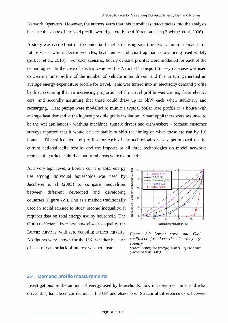
Figure 2-9 Lorenz curve and Gini coefficient for domestic electricity by country ....................... 31
Figure 2-10 Load signatures of washing machines and dishwashers ............................................ 34
Figure 2-11 Average daily lighting profile by season ................................................................... 35
Figure 2-12 Annual consumption by appliance group for 72 houses ........................................... 36
Figure 2-13 Average daily electricity profile per square meter, by house type ............................ 36
Figure 2-14 Correlation of electricity demand with floor area x occupants: Loughborough ....... 37
Figure 2-15 Load duration curve, averaged over 22 houses in Loughborough ........................... 37
Figure 2-16 Range of daily load profiles for clothes drying in 10 identical houses .................... 38
Figure 2-17 Segmentation of users by interest in energy and by income .................................... 44
Figure 3-1 UK Domestic energy use by fuel type and by end use ............................................... 47
Figure 4-1 Typical traces with missing data ................................................................................. 58
Figure 4-2 Annual consumption of the sample Loughborough households ................................. 60
Figure 4-3 Cumulative consumption across sample houses (Lorenz curve) ................................. 61
Figure 4-4 House 6, week 38, 45kWh (autumn 2009) .................................................................. 62
Figure 4-5 House 10, week 9, 79 kWh (winter 2009) ................................................................... 63
Figure 4-6 House 19, week 15, 114 kWh (spring 2008) ............................................................... 63
A Specification for Measuring Domestic Energy Demand Profiles
Page 10 of 120
Figure 4-7 House 17, week 25, 74kWh (summer 2008) ............................................................... 63
Figure 4-8 House 17, week 41, 74 kWh (autumn 2008) ............................................................... 63
Figure 4-9 Summer Tuesday profiles midnight - 4am, House 6 .................................................. 64
Figure 4-10 1-min electricity demand showing characteristic refrigerator cycle ......................... 64
Figure 4-11 Summer Tuesday profiles midnight-4am, House 22 ................................................ 65
Figure 4-12 Summer Tuesday profiles midnight-4am, House 20 ................................................. 65
Figure 4-13 Summer Tuesday profiles midnight-4am, House 9 ................................................... 65
Figure 4-14 8am-midday House 4, Summer Tuesdays .............................................................. 66
Figure 4-15 Evidence of active occupants in the afternoons? ...................................................... 66
Figure 4-16 Summer Tuesday profiles midnight-4 am, House 21 ............................................... 67
Figure 4-17 Summer Tuesday profiles midnight -4am, House 18 ............................................... 67
Figure 4-18 Ordinary tariff users: 1-min resolution average profile ............................................. 67
Figure 4-19 Restricted tariff users: 1-min resolution average profile ......................................... 68
Figure 4-20 All users: 1-min resolution average profile ............................................................... 68
Figure 4-21 Load profile at different resolutions – one house .................................................... 69
Figure 4-22 Load profile at different resolutions – diversified .................................................... 69
Figure 4-23 Individual daily average consumption by week, 2008 .............................................. 70
Figure 4-24 Averaged daily consumption by week, 2008 ............................................................ 70
Figure 4-25 Averaged daily consumption ..................................................................................... 70
Figure 4-26 Ordinary tariff: Comparison with national typical profile ....................................... 71
Figure 4-27 Restricted tariff: Comparison with national typical profile ....................................... 71
Figure 4-28 Electricity consumption per person by household size ............................................ 72
Figure 4-29 Electricity consumption and large appliance ownership .......................................... 72
Figure 6-1 Electricity use in one house by appliance .................................................................... 90
Figure 6-2 Daily electricity consumption ..................................................................................... 91
Figure 6-3 Electricity consumption over 6 days ........................................................................... 91
A Specification for Measuring Domestic Energy Demand Profiles
Page 11 of 120
Figure 6-4 Effect of time averaging data – vacuum cleaner use .................................................. 91
Figure 6-5 Gas usage over 3 days in April ................................................................................... 92
Figure 6-6 Gas demand profile while cooking a meal ................................................................. 92
Figure 6-7 Oil tank gauges in situ, illustrating access challenges ................................................. 93
List of tables
Table 1-1 Growth in UK 1998-2008 ............................................................................................. 13
Table 3-1 Energy use bands based on annual consumption ......................................................... 49
Table 4-1 Number of houses by level of missing data .................................................................. 58
Table 4-2 Distribution of household size compared to national average ...................................... 60
Table 4-3 Distribution of sample houses by Ofgem consumption band ...................................... 61
Table 4-4 Appliance ownership in sample compared to national statistics for 2008 .................... 61
Table 4-5 Ownership of large appliances in top and bottom quartile ........................................... 72
Table 5-1 Instrumentation for full load profile measurement programme .................................... 85
Table 6-1 Electricity end use compared to national statistics ..................................................... 90
Table 6-2 Instrumentation needed and fuel and end use coverage for observation house ............ 94
A Specification for Measuring Domestic Energy Demand Profiles
Page 12 of 120
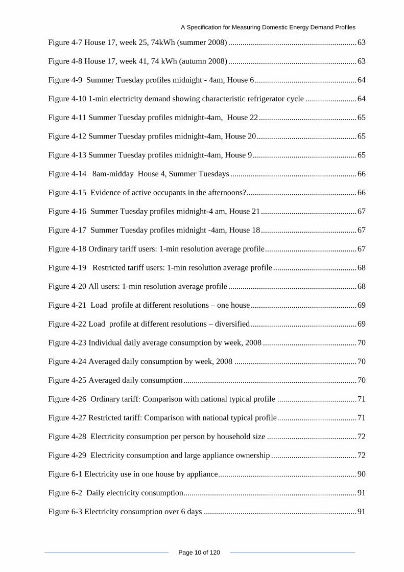
1. Introduction
The world of energy is changing, driven by the need to ensure future security of supply and fears
about the possible impacts of climate change. Intermittent renewable generation from wind, and
eventually waves and tides, is accounting for an increasing proportion of supply, often in
locations far from the centres of demand. Increasing deployment of distributed and micro-
generation is making it more complicated to manage electricity distribution networks. At the
same time, new consumer appliances are offering ever greater possibilities for using more
energy. While new technologies such as heat pumps or electric vehicles may help to reduce
carbon emissions, their spread will cause a large-scale switch from gas or petrol to electricity as
an energy source.
Figure 1-1 UK energy end use 2008 Source: Energy Consumption in the UK - Overall &
Domestic Data Tables (DECC, 2010)
Domestic energy use accounts for 30%
of the UK total; more than half of this is
for space heating (Figure 1-1).
However, there is considerable
geographic variation in fuel type and
usage, especially in Scotland where
large tracts of rural areas have no access
to piped gas and seasonal variations in
daylight are more pronounced.
Appendix 1 illustrates the extent of regional diversity. In Scotland, gas makes up a lower
proportion of all energy use than in the UK as a whole, but the average individual customer uses
more. Glasgow, a city in the central belt, shows similar patterns of fuel usage to central England,
but individual customers consume less gas and electricity – perhaps because of the high
proportion of flats. Argyll & Bute has a limited gas network so much of its heating comes from
other fuels; the high individual gas usage may be related to the fact that it has a low proportion of
people of working age. In Shetland, piped gas is not available at all. By contrast, there is much
less variation between urban and rural areas in central England.
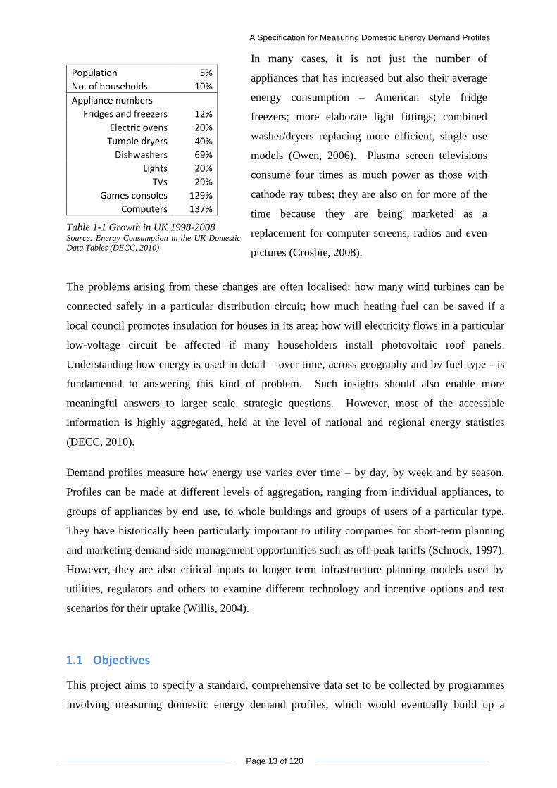
Changes in usage over time have also been quite dramatic. Table 1-1 shows that, over the last 10
years where data is available, the number of electrical appliances has grown faster than either
population or the number of households. This is especially pronounced for consumer electronics
and computers, but also applies to more energy intensive items such as dishwashers and tumble
dryers.
A Specification for Measuring Domestic Energy Demand Profiles
Page 13 of 120
Population 5%
No. of households 10%
Appliance numbers
Fridges and freezers 12%
Electric ovens 20%
Tumble dryers 40%
Dishwashers 69%
Lights 20%
TVs 29%
Games consoles 129%
Computers 137%
Table 1-1 Growth in UK 1998-2008 Source: Energy Consumption in the UK Domestic
Data Tables (DECC, 2010)
In many cases, it is not just the number of
appliances that has increased but also their average
energy consumption – American style fridge
freezers; more elaborate light fittings; combined
washer/dryers replacing more efficient, single use
models (Owen, 2006). Plasma screen televisions
consume four times as much power as those with
cathode ray tubes; they are also on for more of the
time because they are being marketed as a
replacement for computer screens, radios and even
pictures (Crosbie, 2008).
The problems arising from these changes are often localised: how many wind turbines can be
connected safely in a particular distribution circuit; how much heating fuel can be saved if a
local council promotes insulation for houses in its area; how will electricity flows in a particular
low-voltage circuit be affected if many householders install photovoltaic roof panels.
Understanding how energy is used in detail – over time, across geography and by fuel type - is
fundamental to answering this kind of problem. Such insights should also enable more
meaningful answers to larger scale, strategic questions. However, most of the accessible
information is highly aggregated, held at the level of national and regional energy statistics
(DECC, 2010).
Demand profiles measure how energy use varies over time – by day, by week and by season.
Profiles can be made at different levels of aggregation, ranging from individual appliances, to
groups of appliances by end use, to whole buildings and groups of users of a particular type.
They have historically been particularly important to utility companies for short-term planning
and marketing demand-side management opportunities such as off-peak tariffs (Schrock, 1997).
However, they are also critical inputs to longer term infrastructure planning models used by
utilities, regulators and others to examine different technology and incentive options and test
scenarios for their uptake (Willis, 2004).
1.1 Objectives
This project aims to specify a standard, comprehensive data set to be collected by programmes
involving measuring domestic energy demand profiles, which would eventually build up a

A Specification for Measuring Domestic Energy Demand Profiles
Page 14 of 120
consistent picture of how energy use patterns vary over time and across the country. The
methodology began with a literature review to understand the range of uses for energy profiles,
and the experiences of past measurement programmes (Chapter 2). A systematic review was
made of the lessons from published data collection exercises (Chapter 3) and analyses were
made on the one, high-quality data set that was found in the public domain (Chapter 4). A set of
requirements was derived from these, and a standard comprehensive data set to meet the
requirements proposed (Chapter 5). Finally, insights into the practical aspects of such a data
collection exercise were made through observing energy use in one house (Chapter 6).
The scope covers domestic heating, hot water and appliance demand only. Demand profiles for
domestic transport - which could for example be used to model the impacts of charging electric
vehicles at home - have not been considered.
A Specification for Measuring Domestic Energy Demand Profiles
Page 15 of 120
2 Literature review
This section reviews how energy demand profiles are used: for operational support, for
developing and validating energy demand models, and as an input for models that support
decision making on issues ranging from supply-demand balancing and behaviour of networks to
strategic choices about renewable energy technology options. A number of published
measurement programmes are then studied; in particular those made in the UK over the last 10
years, as well as selected examples from elsewhere which illustrate more general lessons on
diversity of behaviours, and experiences with making measurements. The data sets discussed
here are summarised in Appendix 2. Finally, a selection of studies is presented which
investigated how attitudes and behaviours drive energy use.
2.1 Operational support
2.1.1 Scheduling and despatch
Demand forecasting and distribution planning has to be carried out for all fuels, but their varying
characteristics mean that the same activities must be done in different ways and over different
timescales. At the most basic level, a householder who uses solid fuel or oil for heating will
order once or twice a year: since heating oil, coal and wood can be stored safely in the home, it is
not particularly critical that he gets quantities exactly right, or even the timing of the order -
unless of course he has left it until the last minute at the start of a cold snap. Accuracy in volume
and timing becomes more important for transport fuels. Petrol stations typically have storage for
between one day and one week‟s sales, so how demand patterns vary daily, weekly and by
season at each site must be well understood and scheduling is generally centralised (BP, 2009).
In the case of piped gas and electricity, the customer has no storage, and utility companies must
meet demand as it arises. Gas travels through the high-pressure National Transmission System
at around 25 mph (National Grid, 2007) so it is difficult to make effective short-term
interventions if the forecast is wrong. Small fluctuations from forecast volume can be
compensated by varying the line pressure; however, this is costly as it calls for increased use of
compressors (Smith et al, 1996). Demand forecasting is done daily, using measured load shapes
from a small sample of customers for three types of day - weekday, Saturday and
Sunday/holiday; these are combined with long-term statistical correlations between total daily
consumption and weather. This forecasting process is carried out for each of 8 customer
segments across 13 geographical zones. Domestic customers, defined as those who use less than
73 MWh/year, drive most of the weather related variability: on the coldest winter days they
A Specification for Measuring Domestic Energy Demand Profiles
Page 16 of 120
account for 75% of total demand, but less than 25% in the summer (National Grid, 2007). The
average domestic consumption across all gas customers in Great Britain is only 16.9 MWh/year
(DECC, 2010), so it is possible that this one segments contains sub-segments with very different
patterns of use. In countries where gas is less ubiquitously linked to heating, domestic customers
are segmented depending on gas appliances present, and different load shapes are developed for
each segment (Brabec et al, 2009).
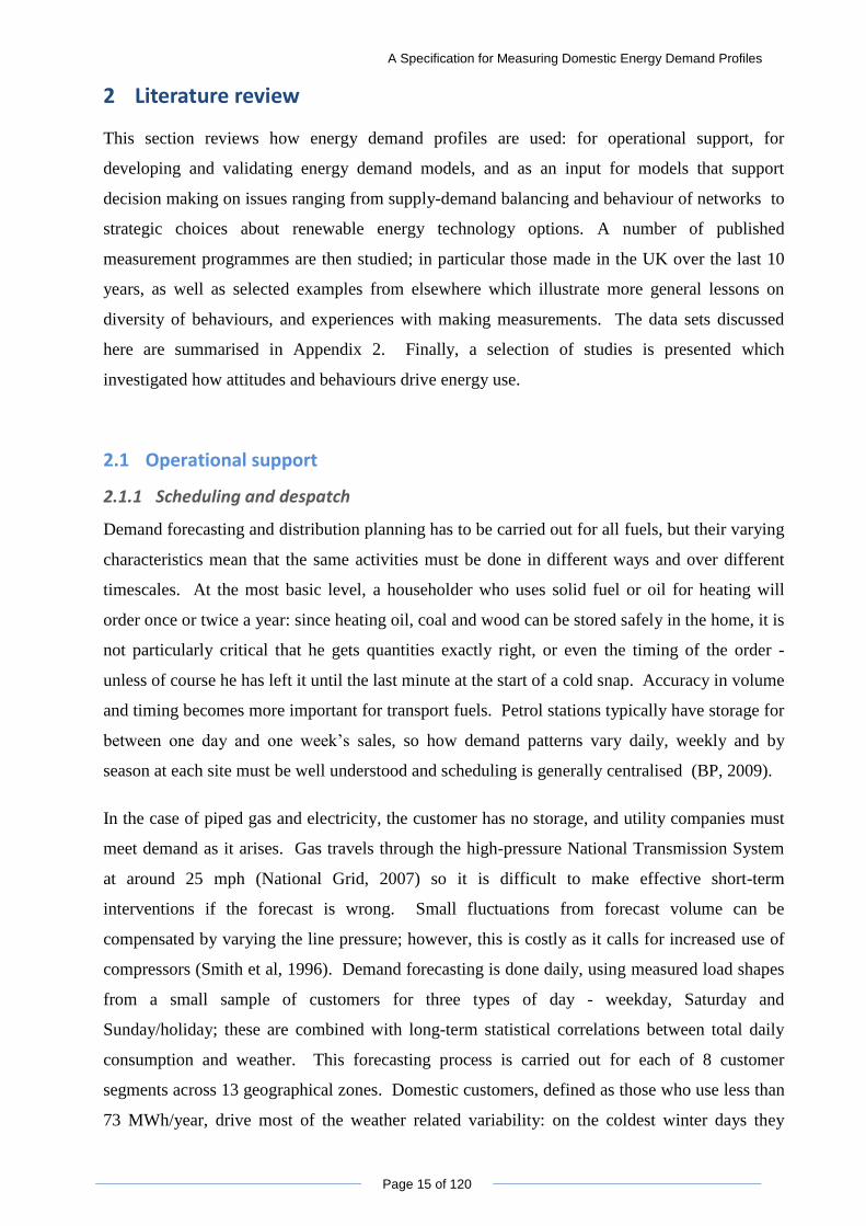
Electricity is particularly sensitive because a momentary mismatch between supply and demand
affects the voltage in the network. Even very short outages can switch off equipment such as
Figure 2-1 UK electricity system forecast and
actual daily profiles Source: New Electricity Trading Arrangements Balancing
Mechanism Reporting
http://www.bmreports.com/bsp/bsp_home.htm, 10 Jun 2011
clocks and computers, and some industrial
applications are affected if the voltage halves
for as little one fifth of a second (Willis,
2004). Supply planning however is done at
much longer intervals. In the UK, electricity
is traded by the half-hour, so the system
operator needs a high-quality forecast of total
demand for each half hour in the year in
order to contract firm and balancing supply
economically (Clark, 2011). Figure 2-1
shows forecast and actual demand profiles
over 3 summer days.
A multitude of mathematical and numerical forecasting methods has been developed for this
purpose, using fuzzy logic, expert systems and neural networks to analyse recent actual overall
daily demand profiles. These are pattern recognition techniques that require minimal inputs –
just day type and temperature - to generate forecasts (Alfares & Nazerruddin, 2002).
Measured half-hourly load profiles are also used for short term distribution planning (Willis,
2004). As part of the national programme to roll out smart meters in small commercial and
domestic customers‟ premises, the Electrical Networks Association recently formulated a
functional specification for smart meters to measure electricity and gas, based on analysing their
envisaged end uses for such data. The highest resolution they specify for electricity is half-
hourly data collection: this would allow monitoring of current flows and voltage levels,
forecasting network loads, and determining demand hidden by microgeneration. For gas
however, they ask for meters to be capable of measuring demand every 6 minutes, for planning
purposes over the winter only (ENA, 2010). It is not altogether clear from the document why
A Specification for Measuring Domestic Energy Demand Profiles
Page 17 of 120
gas would need higher frequency data than electricity.
2.1.2 Settlements
Electricity markets in the UK and elsewhere have been opened up for competition over the last
20 years. Multiple suppliers operate from the same physical infrastructure in any given area, so it
is important to be able to tell who has bought and sold what quantities each half hour. Most sales
are to end customers whose actual usage is metered only at monthly intervals or less, and load
profiling is used to allocate volume, and therefore costs, correctly to suppliers (Bailey, 2000).
Systematic annual collection of half-hourly load profiles from customers in each distribution
region was started in the UK by the Load Research Association in the late 1990s, although
Scotland was included only after 2005. The 29 million non-metered customers are split into 8
different classes: the two domestic classes account for 89% of the number and 69% of the energy
consumed by non-metered customers. Samples are chosen from each class, in each electricity
distribution region, and stratified by high, medium and low users (Elexon, 2011). Half-hourly
consumption is logged over a full year in 2500 premises, with around 10% of these replaced each
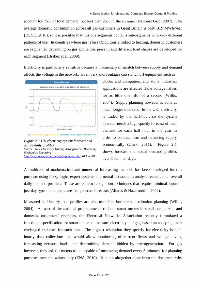
Figure 2-2 Domestic electricity profiles for a winter
weekday Source: Load profiles and their use in electricity settlement (Elexon, 2011)
year for various reasons (K
Spencer, Elexon, personal
communication, 6 April 2011).
For analysis purposes the year is
divided into 5 unequal seasons:
summer is split in two, with a 6-
week „high summer‟ holiday
period. Winter lasts for the entire
period between the October and
March clock changes.
Regression coefficients relating consumption to temperature and day length are calculated for
each half hour in each season, for each day of the week, and for each customer class. A good
estimate of total unmetered volume delivered to the customers of each electricity supplier can
then be built up using the coefficients and their number of customers within each class (Elexon,
2011). Figure 2-2 shows the typical constructed profiles for the two classes of domestic
customers, non-restricted and restricted tariff users.
A Specification for Measuring Domestic Energy Demand Profiles
Page 18 of 120
2.1.3 Managing energy use
Monitoring daily, weekly and annual patterns of energy use can identify opportunities for
reducing consumption. This has mainly been done by facilities managers of commercial and
industrial buildings where energy costs are large. In Leicester, many commercial and public
buildings have half-hourly electricity, gas and water meters connected to a central data gathering
system run by the city council. An analysis of 125 of these over a five year period indicated that
this has led to a significant reduction in heating and in electrical appliances being left on when
the building is unoccupied (Brown et al, 2010). At a smaller scale, one charity halved their gas
consumption after installing an optical character reader which measured their half-hourly usage:
the information allowed them to change the boiler settings to match heating better with
occupancy patterns (Leicester Energy Agency, 2010).
A method of automating benchmarking between commercial buildings was proposed by Ferreira
(2009), who applied a set of coefficients calculated from daily profiles for gas, electricity and
water in 81 different buildings to identify opportunities for saving on utilities in a selection of the
Leicester buildings. The benchmarks included load factors, and other comparisons of mean,
peak and minimum loads in working hours, over the full working day and at weekends
The forthcoming roll-out of smart meters that display half-hourly electricity and gas use presents
the possibility of taking a similar approach at a domestic level. The recently completed Energy
Demand Research Project (EDRP) aimed to understand how effective different forms of
feedback are in reducing or shifting the energy demand of consumers. During the four years that
the programme ran, half-hourly electricity and gas demand was measured in 17000 domestic and
small commercial premises across the UK. It is due to report in the summer of 2011 (Ofgem,
2010).
2.2 Developing and validating energy demand models
Energy demand models range from those which pro-rate based on simple parameters such as
house type, temperature and number of occupants, to ones which aim to simulate the complexity
of real energy flows and human behaviour.
2.2.1 Household energy consumption models
Models for electricity consumption use two approaches. The first is based on measuring actual
load profiles for households, and deriving statistical relationships with possible drivers:
A Specification for Measuring Domestic Energy Demand Profiles
Page 19 of 120
temperature and day length are the main inputs, but floor area and number of occupants are also
commonly used. The second approach builds household level profiles from data on end use,
with some probabilistic overlay to account for different timings in different households.
In Finland, Paatero & Lund (2006) took hourly measured electricity consumption from a set of
702 dwellings – all were apartments in large blocks, which had no electric heating. They
identified and removed daily and weekly cyclical components from the measured profiles, and
compensated for weather. The variation in residual electricity load was considered to represent a
‟social probability factor‟ that any individual household is using any individual appliance at any
one time. The model was then used to estimate the total hourly consumption profile for 10,000
households, assuming that each used an average amount of electricity, and owned an average
number of appliances with average power rating. Although a large number of households were
measured, they were all very similar in type; and a further limitation on the model‟s realism is
the assumption that the „social probability factor‟ is normally distributed and does not vary over
the year.
A similar approach at the end-use level was
taken at de Montfort University in Leicester,
where a 5-minute resolution stochastic
model for lighting was developed from
analysing measured half-hourly lighting
consumption in 100 houses over a full year.
The shape of the average variation was
analysed for each half-hour in the day and
for each season. This shape was very
different over the day – for example, at
Figure 2-3 Annual variation in lighting demand for
one half-hour in the day Source: A simple model of domestic lighting demand (Stokes, Rylatt,
& Lomas, 2004)
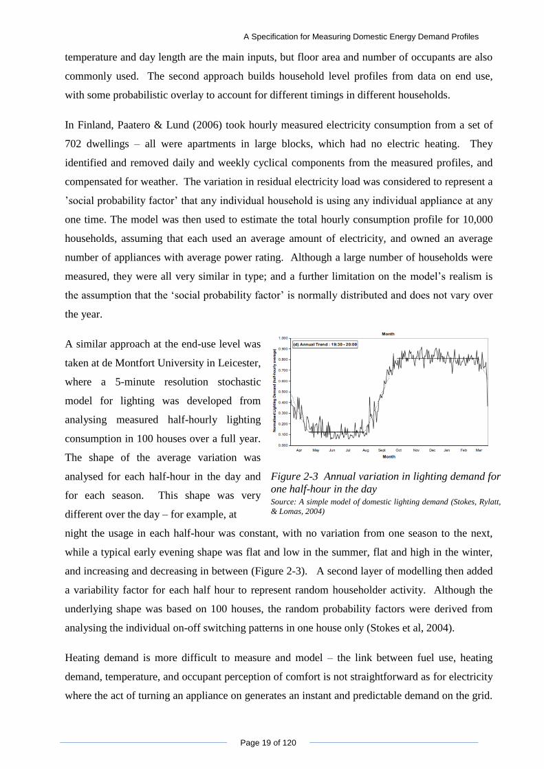
night the usage in each half-hour was constant, with no variation from one season to the next,
while a typical early evening shape was flat and low in the summer, flat and high in the winter,
and increasing and decreasing in between (Figure 2-3). A second layer of modelling then added
a variability factor for each half hour to represent random householder activity. Although the
underlying shape was based on 100 houses, the random probability factors were derived from
analysing the individual on-off switching patterns in one house only (Stokes et al, 2004).
Heating demand is more difficult to measure and model – the link between fuel use, heating
demand, temperature, and occupant perception of comfort is not straightforward as for electricity
where the act of turning an appliance on generates an instant and predictable demand on the grid.
A Specification for Measuring Domestic Energy Demand Profiles
Page 20 of 120
Wind direction, solar gains, and the presence of occupants and appliances which emit heat as a
by-product all affect the internal temperature. The thermal mass of the building and furnishings
can store and release heat, which then alters the time profile of demand on heating fuels. The
BREHOMES energy model has calculated that on average only around half of the useful heat in
housing is supplied directly by heating systems – the rest comes from gains from electric
appliances, water heating losses, and solar and metabolic gains (Shorrock & Utley, 2008).
Yao & Steemers (2005) developed a simplified analytical model to try to predict demand profiles
for all energy used in a typical UK house, based on occupancy patterns and using national
statistics for household size and appliance ownership. Electrical appliance loads, hot water and
heating profiles were modelled for each of five different occupancy patterns. Hot water
consumption was calibrated against measurements of actual quantities of and temperatures of
water used by a three-person family for baths, dish washing and clothes washing; however, no
details were given of the number of data sets or the circumstances these were collected.
Modelled heating demand profiles for three different typical dwellings were used to validate the
heating component of the model rather than measurements; the thermal model used to generate
these had previously been calibrated using a more detailed simulation. Standard, typical
seasonal electricity consumption profiles from the Load Research Association were used to
validate the electricity component.
Hot water demand in South African households was modelled by Lane & Beute (1996), hourly at
community level. Each house was assigned an average-sized hot water cylinder and total daily
demand. The time profile was split into five elements: a high morning load; a high evening load;
a moderate midday load; plus small unpredictable and standby loads which varied only slightly
through the working day. Within each element a normal distribution was assumed for the on-off
timing of an individual household‟s hot water tank. These distributions were based on surveys
on the timing of hot-water using activities in an unstated number of houses, together with 15-
minute measurements of the electricity supply to the hot water cylinder; however, these
measurements lasted only 14 days. The authors calibrated the model against total hot water load
profile measurements from utility companies supplying three different communities in S Africa.
Each community had a similar population, and each exhibited a similar overall demand profile
which agreed well with the model prediction. The size of the peaks was around +/-10% different
to the model, and the timing varied by +/- 1hr.
Heating demand models have also been built using expert systems and neural networks to search
for patterns and correlations within measured data. In Sweden, a neural network model to
A Specification for Measuring Domestic Energy Demand Profiles
Page 21 of 120
estimate daily heating demand was trained using measurements in 8 houses over 2 years; these
were reported to included indoor and outdoor temperatures and energy demand for space and
water heating (Olofsson et al, 1998). Yu et al (2010) developed a decision tree model for
predicting overall energy demand for buildings in Japan; this claimed to have used data from 55
residential buildings to train the model, and a further 12 to calibrate it. Inputs included
measurements of indoor environment at 15 minute intervals and of energy use for each type of
fuel, as well as socio-economic data collected on the households involved, their appliances and
energy related behaviours. In Korea, a Community Energy System design toolkit is being
developed which includes a model to generate the hourly demand profile for electricity, heating,
cooling and hot water in a group of buildings. The input for this was reported to be statistical
correlations metered daily electricity and gas consumption for a large number of buildings,
together with 3-5 minute resolution measurements for a sample of buildings in different cities
(Chung & Park, 2010). None of these papers however gives any detail about the actual
measurements made or what the profiles looked like.
2.2.2 Energy demand simulation
Simulation, as opposed to modelling, attempts to mimic the complexity of the real world, and
generate more realistic results than the simple models described above. However, validating
simulations against measurements is challenging because not only the outputs need to be
compared but also the inputs, and at this level of detail measurement error may be just as
significant as modelling error.
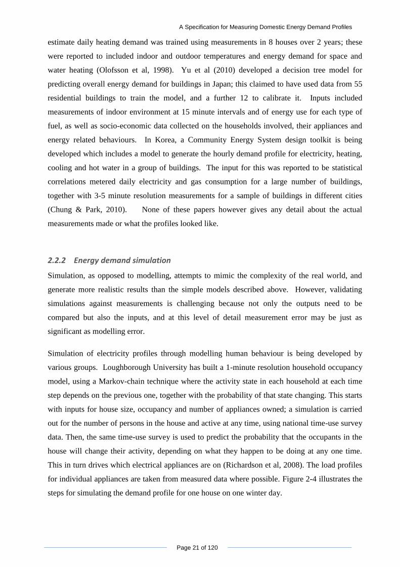
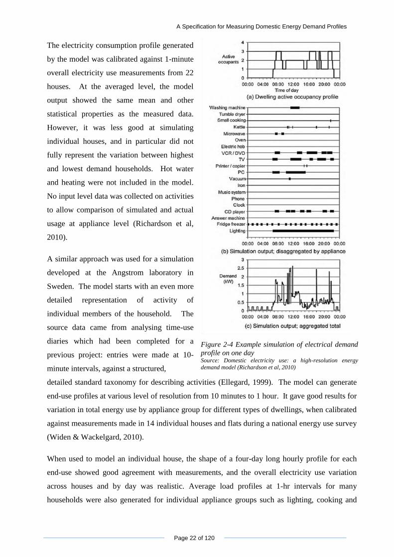
Simulation of electricity profiles through modelling human behaviour is being developed by
various groups. Loughborough University has built a 1-minute resolution household occupancy
model, using a Markov-chain technique where the activity state in each household at each time
step depends on the previous one, together with the probability of that state changing. This starts
with inputs for house size, occupancy and number of appliances owned; a simulation is carried
out for the number of persons in the house and active at any time, using national time-use survey
data. Then, the same time-use survey is used to predict the probability that the occupants in the
house will change their activity, depending on what they happen to be doing at any one time.
This in turn drives which electrical appliances are on (Richardson et al, 2008). The load profiles
for individual appliances are taken from measured data where possible. Figure 2-4 illustrates the
steps for simulating the demand profile for one house on one winter day.
A Specification for Measuring Domestic Energy Demand Profiles
Page 22 of 120
The electricity consumption profile generated
by the model was calibrated against 1-minute
overall electricity use measurements from 22
houses. At the averaged level, the model
output showed the same mean and other
statistical properties as the measured data.
However, it was less good at simulating
individual houses, and in particular did not
fully represent the variation between highest
and lowest demand households. Hot water
and heating were not included in the model.
No input level data was collected on activities
to allow comparison of simulated and actual
usage at appliance level (Richardson et al,
2010).
A similar approach was used for a simulation
developed at the Angstrom laboratory in
Sweden. The model starts with an even more
detailed representation of activity of
individual members of the household. The
source data came from analysing time-use
diaries which had been completed for a
previous project: entries were made at 10-
minute intervals, against a structured,
Figure 2-4 Example simulation of electrical demand
profile on one day Source: Domestic electricity use: a high-resolution energy
demand model (Richardson et al, 2010)
detailed standard taxonomy for describing activities (Ellegard, 1999). The model can generate
end-use profiles at various level of resolution from 10 minutes to 1 hour. It gave good results for
variation in total energy use by appliance group for different types of dwellings, when calibrated
against measurements made in 14 individual houses and flats during a national energy use survey
(Widen & Wackelgard, 2010).
When used to model an individual house, the shape of a four-day long hourly profile for each
end-use showed good agreement with measurements, and the overall electricity use variation
across houses and by day was realistic. Average load profiles at 1-hr intervals for many
households were also generated for individual appliance groups such as lighting, cooking and
A Specification for Measuring Domestic Energy Demand Profiles
Page 23 of 120
computer use and compared well to equivalent measurements in 217 households, although the
modelled peaks were generally higher than the measured. Load profiles for hot water were
compared against 10-min resolution measurements in 10 households over a 9-month period, but
these showed less agreement. The authors speculated that some of the differences could be due
to the fact that the time-use data was collected more than a decade before the energy
consumption profiles and that household appliances and habits may have changed since then
(Widen et al, 2009). This model has used a broader range of data for validation than any other
reviewed, but at a resolution one-tenth as fine as in the Loughborough study.
In the case of heating, where demand profiles are difficult to measure directly, simulations are
often used rather than measurements to validate simpler models. Building simulation programs
model the complex interactions of heat flow, air flow and light, with changes in weather,
occupancy patterns, heating and cooling system settings, in a building of a given location,
geometry and construction detail. ESP-r is a simulation program at the University of Strathclyde
that has been used by others to produce or validate heating demand profiles for their own models
such as Yao & Steemers (2005).
The ESP-r program starts with a detailed model of the building under study: its size, layout and
orientation. The materials that make up the fabric are modelled in detail, with the
thermodynamic properties of each layer in each wall described separately, in addition to the
optical properties of each transparent surface. Casual gains from occupants, lights and other
electrical equipment are modelled as a function of time. Variations in weather induced heating,
cooling, and lighting are modelled using a climate profile consisting of time series data for wind
speed and direction, direct and diffuse solar radiation, and relative humidity. The building is
split into a series of connected discrete volumes. Partial differential equations are set up to
describe conductive, convective and radiative heat flow and mass flow between each pair of
volumes at one point in time; a measured climate profile supplies the changing external
boundary conditions. The simultaneous differential equations are solved numerically for each
time step by a finite difference technique. An air flow network for fluid flow, an electrical
network and a separate HVAC network can also be included, each tied into the building by a
series of nodes at critical locations. This method allows realistic modelling of interactions, such
as changes in convection coefficient with temperature, or the impact of changing external light
levels on the air temperature and hence on energy demand for heating or cooling (Clarke, 2001).
However, electrical demand from appliances is not simulated at the same level of detail.
A history of the validation tests carried out on ESP-r was reported by Strachan et al (2006). In
A Specification for Measuring Domestic Energy Demand Profiles
Page 24 of 120
addition to validating the program itself by code checking and analysis, comparisons were made
with other programs and with measured data from test houses. Early comparisons included two
houses in Livingston, Scotland where air and surface temperatures were measured with 24
sensors per house, and air infiltration was measured with tracer gas; and two houses in Australia.
In each case one out of the two houses agreed better with prediction than the other. Experiments
were carried out in a test environment to calibrate individual parts of the model, such as: a
double glazed window in an insulated wall; a conservatory; a Trombe wall. Under these
controlled circumstances, measured and predicted temperatures agreed to within 0.56C. Another
set of comparisons were carried out against measurements in a house in Lisses, France.
Measured and simulated energy consumption over two winter months agreed to -4% to +26% for
the whole house, but less well in detail for individual floors. This was thought to be because
actual air movements in the hallway moved a greater amount of heat from the ground floor to the
first than in the simulation.
Calibrating such models against real consumption is difficult because the process is detailed and
intrusive in terms of instrumentation required, and may need to be done without people actually
present. However, heating demand is influenced by human behaviour as well as by climate and
thermal properties, which adds even more complexity to a simulation. An example is a module
that has been developed for ESP-r to simulate window opening behaviour. Thermal comfort data
were collected from occupants in 15 office buildings in Oxford and Aberdeen. 890 people were
surveyed one day a month over 6 months about their comfort level, clothing, and use of building
controls including windows. 219 of those surveyed completed a detailed record of these factors,
4 times each day for 3 months; and temperature was logged near their work area and outside.
This data was used to build a model of window-opening behaviour based on the difference
between indoor and outdoor temperature (Rijal et al, 2007).
2.3 Inputs for other modelling
Demand profiles are used as inputs for other types of model; directly measured profiles are used
in some cases but modelled ones are also used. This section describes a number of examples
illustrating different approaches, but is not intended as a literature review on modelling in
general.
2.3.1 Supply-demand balance with renewable and distributed generation
The need to understand heating demand profiles in detail has been accelerated by the
development of CHP systems, as these must be matched to a combined heating and electricity
A Specification for Measuring Domestic Energy Demand Profiles
Page 25 of 120
demand. Veitch & Mahkamov (2009) modelled daily energy demand for a typical semi-
detached house at 1-minute resolution in order to test the performance of a pre-production model
of a micro-CHP system in a laboratory; measurements included the gas consumption, heat
output, and the emissions in the exhaust gases. The simplified modelling approach was very
similar to that of Yao & Steemers (2005); however, additional refinements were made to model
the differences between weekdays and weekends, and seasonality. The model generated a
consistent set of heating, hot water and electricity demand profiles for the test, although the
conditions were limited to one location (SE England), one house with one occupancy pattern,
using one set of appliances. The modelled profile was calibrated only against national statistics
on annual gas and electricity use.
An operational application for using load profiles in a CHP system was tested by Bakker et al
(2008). The controller for the micro CHP system of a single house was set up to record time
series data on production, thermostat settings and weather. It used these measurements to
generate an hourly profile of heat demand for the day ahead, using a neural network to analyse
the previous few days‟ records, by day type. This was tested with data from 4 houses in
Netherlands, where a year‟s worth of 1-minute measurements on hot water tank and µCHP
appliance status had been measured by the Dutch utility company. The controller was able to
predict the shape of the profile quite well in each case, although the magnitude of the predicted
heat demand could be +/-25% different to the measured. The measurement data were not
described in detail.
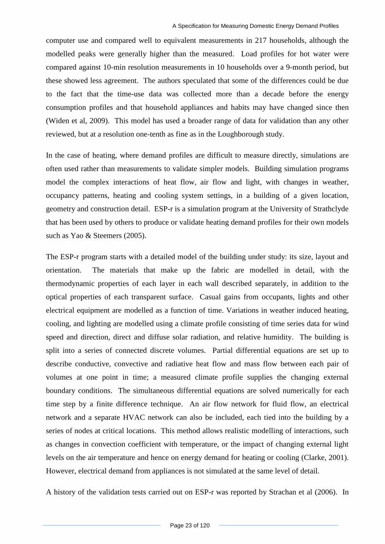
Hawkes & Leach (2005)
investigated the impact of using load
profiles at different time steps on
models to determine the optimised
operation of a CHP system. For
electricity, they reported using 5-
minute demand profiles measured by
BRE on 3 houses. However, they
could not find any equivalent data on
heating demand, so they made one
set of measurements themselves at
Figure 2-5 Daily heat demand profile used to model CHP
system Source: Impacts of temporal precision in optimisation modelling of
micro-Combined Heat and Power (Hawkes & Leach, 2005)
5-min intervals on a winter day and used that for all simulations – see Figure 2-5. Using this
limited data set, the authors concluded that if the time step used is greater than 10 minutes, it
leads to undersized systems and overestimation of CO2 reduction.
A Specification for Measuring Domestic Energy Demand Profiles
Page 26 of 120
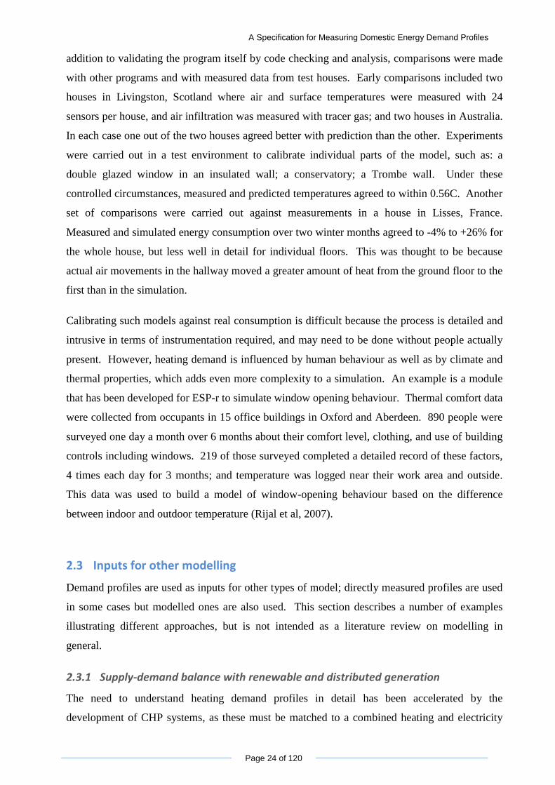
Jenkins et al (2009) used the
measured hourly thermal demand
profiles from one house to estimate
the cost and carbon savings from
using a ground source heat pump to
replace a gas boiler. The data were
reported to have been sourced from
Newborough & Augood (1999),
although the cited reference does
not actually include the data which
is reproduced in Figure 2-6. One
issue they found with the data was
Figure 2-6 Hourly measured thermal demand for a UK
house Source: Modelling the carbon-saving performance of domestic ground-
source heat pumps (Jenkins et al , 2009)
that hot water and heating demand could not be distinguished. They therefore had to assume that
both were supplied at the same water output temperature – although in reality hot water must be
stored at a minimum of 60⁰C in order to guard against Legionella disease, whereas a heat
pump‟s output is between 35-55⁰C; this led to an over-estimate the CO2 savings.
Figure 2-7 Annual electricity profiles for 40 houses with
CHP system Source: Vuillecard et al (2011): small scale impact of gas technologies
on electric load management
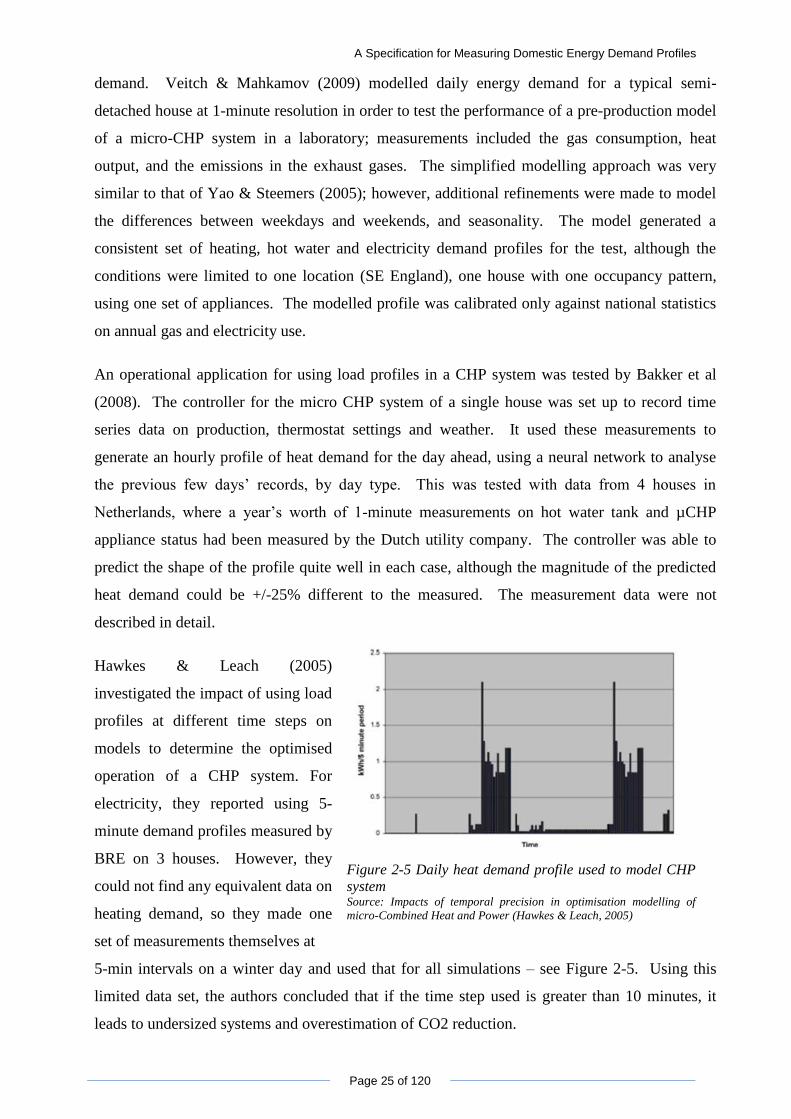
Vuillecard et al (2011) looked at the
impact of domestic micro-CHP systems
on reducing peak electrical load. They
used measurements from 40 houses with
CHP systems in Southeast France,
collecting a year‟s worth of 1-minute
resolution data on: electricity generation,
import and export; gas and hot water
consumption; indoor and outdoor
temperature, as well as hot water tank
temperature. Information was also
collected on house size and year of construction, as well as occupancy patterns, in order to see
how typical of the local population their sample group was. They observed an increase in
electricity demand over the winter, but this was more than counterbalanced by the increased
electricity production from CHP plants in the cold season. Overall, the effect of CHP system
was to redcue peak load for the group by 17%. They also used this data to model the impact of
other technologies on peak load, such as heat pumps and Joule heaters.
A Specification for Measuring Domestic Energy Demand Profiles
Page 27 of 120
Hawkes (2011) showed that timing effects are also important when assessing carbon savings of
demand-side management and microgeneration technologies. He calculated the half-hourly CO2
intensity of the UK generation mix as it varied with demand through the day, and showed that
the actual carbon savings from heat pumps fall dramatically at times when the grid carbon
intensity is high, whereas those from fuel cell CHP systems rises.
Chen & Lee (2010) looked at the fuel savings available from using rejected condenser heat from
air conditioners to preheat domestic hot water in Hong Kong. They constructed daily hot water
demand from measurements of incoming water temperature, shower temperature and flow rate in
36 flats over a 3-month period in the winter, together with information about daily occupancy
and air conditioning use patterns. Using this limited information they calculated potential heat
recovery in different seasons, and estimated that the air-conditioners are able to supply hot water
needs for around two-thirds of the year.
Hong et al (2011) used ESP-r to examine the extent to which thermal storage available in the
fabric of a typical UK detached house could allow an air-source heat pump to be operated
outside peak electrical demand periods without impacting occupant comfort – defined simply as
air temperatures over 18⁰C and water over 40⁰C. They modelled heat flows in a house during
one winter week under four different conditions: with standard and elevated temperature settings
for the heat pump switch, plus the introduction of two different hot water tanks for thermal
buffering. A 1-minute time step was used to model the heat flows, temperatures, and demand on
the heat pump at an appropriate level of resolution.
The integration of solar photvoltaic systems with household energy use was investigated by Firth
et al (2009). They used 5-minute resolution measurements of electricity generated by the PV
system, and electricity imported and exported to the grid, to derive household demand profiles
and analyse what types of household would benefit most from installing such technology. Here
again the time resolution used made a difference to the estimated ability to provide the
household‟s needs from on-site generation: although average demand and average supply from
the PV system could look balanced over half an hour, this could mask large fluctuations with a
high-short term demand on the grid followed by a short period of export (Wright & Firth, 2007).
A tool for modelling renewable energy generation matching with demand over time was
developed at the University of Strathclyde. MERIT can model the generation profiles of various
technologies such as wind, solar and CHP, from a time series climate profile. Auxiliary
technologies such as batteries for storage, or standby generators, can also be added. These can
A Specification for Measuring Domestic Energy Demand Profiles
Page 28 of 120
then be matched to demand profiles for electricity, heating and hot water. Diversified demand for
larger groups of houses and businesses can be built up from individual profiles (Born et al,
2001a). This tool was used to evaluate whether a small island community could become 100%
self-sufficient in energy through a combination of wind and biodiesel from energy crops. The
electricity demand profiles used the Load Research Group‟s standard, average half hourly load
shapes for electricity, scaled to meet typical annual consumption for buildings of that type, and
estimates for heating demand based on occupancy (Born et al, 2001b).
A combination of ESP-r and MERIT was used to develop hybrid renewable energy system
options for a large apartment block in Korea: heating and cooling demand for one vertical block
of apartments was modelled in detail in ESP-r; electricity and hot water demand were reported to
be based on measurements in similar apartments; and a half-hourly demand profile for the whole
block was modelled from combinations of these using an information management tool, EnTrak.
The overall profile was then imported to MERIT, where various combinations of renewable
energy technologies could be assessed to see which gave the closest match (Clarke et al, 2005).
In all these cases the usefulness of the outputs depends on the quality of the input demand
profiles.
2.3.2 Behaviour of electricity distribution networks
Detailed electricity demand profiles are becoming more commonly used for network planning as
this gives possibilities for getting more out of existing distribution systems than current design
practice allows. The basic design parameter for sizing distribution networks is the expected
contribution of each individual consumer to the maximum overall load in the network, called
„After Diversity Maximum Demand‟ (ADMD). As the number of consumers on the network
increases, the contribution of each to the overall peak goes down because each individual
customer‟s peak will occur at a slightly different time. If there are more than around 100 similar
customers, the average load per customer at the peak approaches a constant figure which is
approximates to ADMD (Willis, 2004). The actual value varies by customer area and has to be
established empirically, so utilities use appropriate historical ADMD values for network
planning. 2kW is commonly used in the UK for domestic premises without electric heating
(Central Networks Design Manual, cited by Richardson (2010)).
McQueen et al (2004) argued that the ADMD formulae in use in New Zealand are conservative.
They used measured 1-minute resolution demand data from 21 houses to construct a probabilistic
model that would allow better estimates. The model‟s predicted load distribution compared well
A Specification for Measuring Domestic Energy Demand Profiles
Page 29 of 120
against 10-minute load measurements at one transformer for one month, and the predicted
maximum loading over the whole year was only 2% higher than the measured. However, the
data used to build the simulation was measured over only 2 weeks. Also, the comparison
transformer was from the same geographical area – possibly, although not clear from the paper,
on the same network. A further comparison was made of the predicted and actual 10-year
maximum on each phase of each of 557 transformers in different city, and here there was a
considerable scatter in the outcomes, with predicted phase load if anything slightly lower than
actual on average.
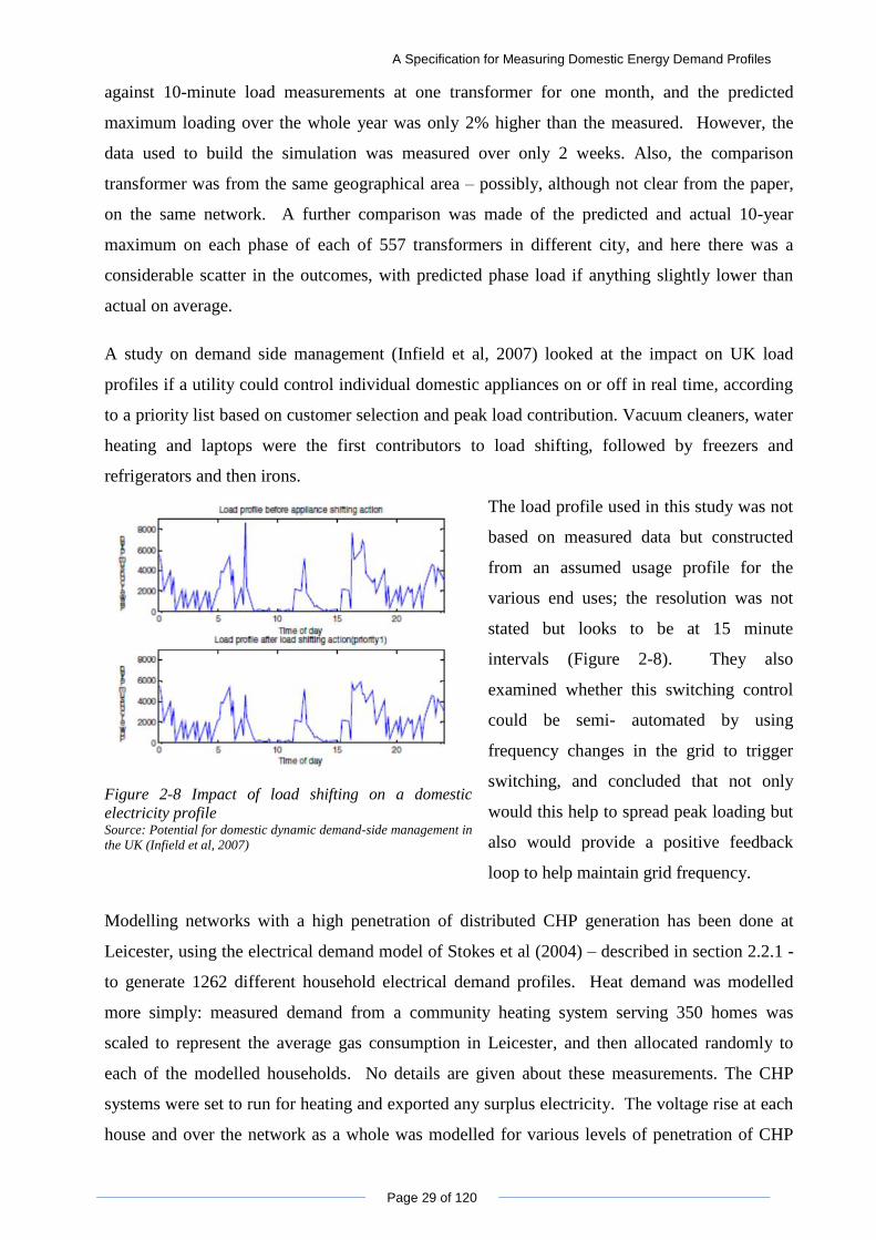
A study on demand side management (Infield et al, 2007) looked at the impact on UK load
profiles if a utility could control individual domestic appliances on or off in real time, according
to a priority list based on customer selection and peak load contribution. Vacuum cleaners, water
heating and laptops were the first contributors to load shifting, followed by freezers and
refrigerators and then irons.
Figure 2-8 Impact of load shifting on a domestic
electricity profile Source: Potential for domestic dynamic demand-side management in
the UK (Infield et al, 2007)
The load profile used in this study was not
based on measured data but constructed
from an assumed usage profile for the
various end uses; the resolution was not
stated but looks to be at 15 minute
intervals (Figure 2-8). They also
examined whether this switching control
could be semi- automated by using
frequency changes in the grid to trigger
switching, and concluded that not only
would this help to spread peak loading but
also would provide a positive feedback
loop to help maintain grid frequency.
Modelling networks with a high penetration of distributed CHP generation has been done at
Leicester, using the electrical demand model of Stokes et al (2004) – described in section 2.2.1 -
to generate 1262 different household electrical demand profiles. Heat demand was modelled
more simply: measured demand from a community heating system serving 350 homes was
scaled to represent the average gas consumption in Leicester, and then allocated randomly to
each of the modelled households. No details are given about these measurements. The CHP
systems were set to run for heating and exported any surplus electricity. The voltage rise at each
house and over the network as a whole was modelled for various levels of penetration of CHP
A Specification for Measuring Domestic Energy Demand Profiles
Page 30 of 120
systems (Thomson & Infield, 2008). A network-level study on the effect of large-scale
deployment of household level PV systems was carried out by Richardson et al (2009). Using
the 1-minute resolution Loughborough model described in section 2.2.2, they simulated
electricity demand profiles for 35,000 households and aggregated them to represent the total for
a network.
A large-scale model of a suburban distribution network with several thousand houses and many
PV, micro-wind and –CHP installations was studied by Burt et al (2008). ESP-r was used to
simulate the net electrical demand profile of 24 individual houses with different occupancy
patterns and types of microgeneration, at 5-minute time steps. These net demand profiles were
then combined, with slight variations in timing and scaling, to represent a diversified aggregated
demand for an entire 11kV circuit with 5 secondary substations. This gives a good model of
overall energy demand including heating, although the electrical appliance model was less
detailed than those used by Thomson & Infield (2008) or Richardson et al (2009).
Sulka & Jenkins (2008) built a simple, integrated model of an estate of houses each equipped
with a Stirling engine CHP system, and linked to the same electric feeder. They investigated the
effect on the overall power flows of various house types and temperature settings. The model
generated hourly demand profiles for each house, using a simplified thermodynamic model of
that house type with a hot water tank in it, together with a separate electrical model based on
random assignments of one of five types of occupancy pattern. Hot water demand was modelled
based on one set of measurements, apparently the same as that used by Yao & Steemers, 2005).
Active network management is being trialled in Orkney, with the aim of allowing a higher
proportion of wind turbines to be connected to the grid provided that some of them can be
switched off if the supply exceeds demand (Currie et al, 2006). However, the economics of
running a plant under such „regulated non-firm generation‟ rules depends critically on how much
down time they may expect. This in turn requires good understanding of the variability of local
demand profiles; the methodology described in the paper requires historical, half-hourly, local
load demand data.
2.3.3 Decision support for policy changes
A University of Edinburgh study on the potential for renewable electricity generation in Scotland
looked at supply and demand projections geographically by Grid Supply Point (GSP). They
approximated geographic variation in using the maximum recorded demand at each GSP
transformer to scale the overall daily profile supplied by each of the two Scottish Transmission
A Specification for Measuring Domestic Energy Demand Profiles
Page 31 of 120
Network Operators. However, the authors warn that this introduces inaccuracies into the analysis
because the shape of the load profile would generally be different at each (Boehme et al, 2006).
A study was carried out on the potential benefits of using smart meters to control demand in a
future world where electric vehicles, heat pumps and smart appliances are being used widely
(Strbac, et al., 2010). For each scenario, hourly demand profiles were modelled for each of the
technologies. In the case of electric vehicles, the National Transport Survey database was used
to create a time profile of the number of vehicle miles driven, and this in turn generated an
average energy expenditure profile for travel. This was turned into an electricity demand profile
by first assuming that an increasing proportion of the travel profile was coming from electric
cars, and secondly assuming that these could draw up to 6kW each when stationary and
recharging. Heat pumps were modelled to mimic a typical boiler load profile in a house with
average heat demand at the highest possible grade insulation. Smart appliances were assumed to
be the wet appliances - washing machines, tumble dryers and dishwashers - because customer
surveys reported that it would be acceptable to shift the timing of when these are run by 1-6
hours. Diversified demand profiles for each of the technologies was superimposed on the
current national daily profile, and the impacts of all three technologies on model networks
representing urban, suburban and rural areas were examined.
At a very high level, a Lorenz curve of total energy
use among individual households was used by
Jacobson et al (2005) to compare inequalities
between different developed and developing
countries (Figure 2-9). This is a method traditionally
used in social science to study income inequality; it
requires data on total energy use by household. The
Gini coefficient describes how close to equality the
Lorenz curve is, with zero denoting perfect equality.
No figures were shown for the UK, whether because
of lack of data or lack of interest was not clear.
Figure 2-9 Lorenz curve and Gini
coefficient for domestic electricity by
country Source: Letting the (energy) Gini out of the bottle
(Jacobson et al, 2005)
2.4 Demand profile measurements
Investigations on the amount of energy used by households, how it varies over time, and what
drives this, have been carried out in the UK and elsewhere. Structural differences exist between
A Specification for Measuring Domestic Energy Demand Profiles
Page 32 of 120
countries, as different climates drive very different heating and cooling needs, and normal
working hours vary from country to country. Fuel use is linked to different end-uses in each
country: in the UK, where piped gas is available, it is used for heating as well as cooking
(DECC, 2010); in parts of East Europe where the standard form of heating is district heating in
apartment blocks (Brabec et al, 2009) or in France where nuclear electricty is cheap
(REMODECE, 2008) this is not always the case. Cultural factors also come into play, such as
the fact that southern Chinese cooking uses very high amounts of gas for stir-frying (Chen &
Lee, 2010). This section therefore looks in detail at a number of UK energy demand
measurement programmes, and at selected examples from outside the UK which illustrate
general lessons on diversity of behaviours, and experiences with making measurements. The
studies are compared in tabular form in Appendix 2.
2.4.1 UK studies
An important study on how overall energy use has changed over time was carried out on a group
of 36 low-energy houses in Milton, Keynes. It compared energy use in 1989-91 when the houses
were newly built, with that 15 years later (Summerfield et al, 2010). In the original programme,
temperature and relative humidity (RH) were measured hourly in the living room and main
bedroom, as well as gas and electricity consumption and weather data. In the follow-up, only
temperature and RH were monitored at that resolution, although gas and electricity meters were
read at weekly or fortnightly intervals. Social surveys of the households were carried out on
both occasions; however, the data from the earlier study had been lost. The authors reported that
the original groupings of low, medium and high users remained the same 15 years later. The
high users had increased their consumption to a much greater extent than the medium and low
energy groups. Heating still used the same amount of energy per unit floor area as in the original
study, but the high users had built extensions which increased their total consumption. Average
indoor temperatures had not changed over the period, although the authors point out that these
were well-built, low-energy houses to begin with (Summerfield et al, 2007). Electricity use had
however gone up, by 72% among the high users, although less significantly in the middle and
low use groups.
Shipworth et al (2010) published the results of a survey on reported and estimated central heating
use in 427 homes across England and Wales. Estimated thermostat setting and heating hours
were derived from temperature sensors installed in the living rooms and bedrooms between July
and February. The readings from these were compared with people‟s reported thermostat
settings and heating hours. The estimated average setting was 21⁰C, but there was some
A Specification for Measuring Domestic Energy Demand Profiles
Page 33 of 120
variation: 44% of households were over 22⁰C while 30% were at 20⁰C or less. They found that
householders consistently under-estimated their thermostat settings, with the mean reported
values around 2⁰C lower than measured, although there was enormous individual variability.
People‟s estimates of the length of time that the central heating systems were run were closer to
that deduced from the sensor measurements. Although the trends were clear, there was some
uncertainty about how significant the size of the difference was, as the sensors were put in place
by the occupants themselves and there was no way of checking whether it was the right location.
Energy and water use in low carbon, affordable housing heated with a biomass district heating
system was monitored over 15 months by Gill et al (2011). The buildings belonged to a housing
association and comprised one-bedroom flats and two-and three-bedroom houses. Electricity
and hot water meters were read „periodically‟ for all the houses; only 4 had detailed, 10-minute
logging of electrical load, water volumes and heat input, as well as temperature and relative
humidity in the kitchen/living area. These houses consumed 43% less energy and 52% less
carbon per unit area than the national average. However, compared to other low-energy houses
they did use 11% more electricity because they had forced rather than natural ventilation.
There was considerable variation in the total energy used per house: the highest consumer had
double the usage per square meter of the lowest. Considering space heating alone, the highest
consumer used more than three times as much energy per square meter as the lowest; this was
because of individual differences in thermostat settings. When two of the houses with detailed
monitoring were compared, a reduction of 1.5⁰C in average internal winter temperature resulted
in around 38% less energy for space heating for the same floor area. Electricity consumption
per person decreased with increasing numbers of occupants, because appliances such as lights
can be shared. As in the Milton Keynes study, the high users of space heating were high users of
hot water and electricity as well. Among the four houses with detailed monitoring, the one with
the highest space heating per unit area also used the highest amount of hot water per person; and
the two higher heating users were also the two which used the most electricity, and showed the
highest peak loads. Hot water usage varied more than two-fold, between 19.0 and 47.1 litres per
person per day. This compares with the average use of 26.4 l per person per day quoted in Yao &
Steemers (2005) – excluding clothes and dish washing - assuming that these new houses had
washing machines and dishwashers with cold water intakes.
Newborough & Augood (1999) measured electricity profiles in 30 houses in an investigation of
the potential to shift the timing of appliances that make a large contribution to peak load.
Average power and power factor were logged at 1-minute intervals for a period between 1-4
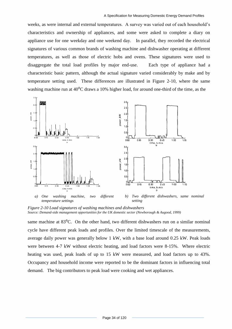
A Specification for Measuring Domestic Energy Demand Profiles
Page 34 of 120
weeks, as were internal and external temperatures. A survey was varied out of each household‟s
characteristics and ownership of appliances, and some were asked to complete a diary on
appliance use for one weekday and one weekend day. In parallel, they recorded the electrical
signatures of various common brands of washing machine and dishwasher operating at different
temperatures, as well as those of electric hobs and ovens. These signatures were used to
disaggregate the total load profiles by major end-use. Each type of appliance had a
characteristic basic pattern, although the actual signature varied considerably by make and by
temperature setting used. These differences are illustrated in Figure 2-10, where the same
washing machine run at 40⁰C draws a 10% higher load, for around one-third of the time, as the
a) One washing machine, two different
temperature settings
b) Two different dishwashers, same nominal
setting
Figure 2-10 Load signatures of washing machines and dishwashers
Source: Demand-side management opportunities for the UK domestic sector (Newborough & Augood, 1999)
same machine at 83⁰C. On the other hand, two different dishwashers run on a similar nominal
cycle have different peak loads and profiles. Over the limited timescale of the measurements,
average daily power was generally below 1 kW, with a base load around 0.25 kW. Peak loads
were between 4-7 kW without electric heating, and load factors were 8-15%. Where electric
heating was used, peak loads of up to 15 kW were measured, and load factors up to 43%.
Occupancy and household income were reported to be the dominant factors in influencing total
demand. The big contributors to peak load were cooking and wet appliances.
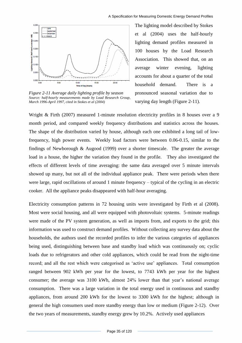
A Specification for Measuring Domestic Energy Demand Profiles
Page 35 of 120
Figure 2-11 Average daily lighting profile by season Source: half-hourly measurements made by Load Research Group,
March 1996-April 1997, cited in Stokes et al (2004)
The lighting model described by Stokes
et al (2004) uses the half-hourly
lighting demand profiles measured in
100 houses by the Load Research
Association. This showed that, on an
average winter evening, lighting
accounts for about a quarter of the total
household demand. There is a
pronounced seasonal variation due to
varying day length (Figure 2-11).
Wright & Firth (2007) measured 1-minute resolution electricity profiles in 8 houses over a 9
month period, and compared weekly frequency distributions and statistics across the houses.
The shape of the distribution varied by house, although each one exhibited a long tail of low-
frequency, high power events. Weekly load factors were between 0.06-0.15, similar to the
findings of Newborough & Augood (1999) over a shorter timescale. The greater the average
load in a house, the higher the variation they found in the profile. They also investigated the
effects of different levels of time averaging: the same data averaged over 5 minute intervals
showed up many, but not all of the individual appliance peak. There were periods when there
were large, rapid oscillations of around 1 minute frequency – typical of the cycling in an electric
cooker. All the appliance peaks disappeared with half-hour averaging.
Electricity consumption patterns in 72 housing units were investigated by Firth et al (2008).
Most were social housing, and all were equipped with photovoltaic systems. 5-minute readings
were made of the PV system generation, as well as imports from, and exports to the grid; this
information was used to construct demand profiles. Without collecting any survey data about the
households, the authors used the recorded profiles to infer the various categories of appliances
being used, distinguishing between base and standby load which was continuously on; cyclic
loads due to refrigerators and other cold appliances, which could be read from the night-time
record; and all the rest which were categorised as „active use‟ appliances. Total consumption
ranged between 902 kWh per year for the lowest, to 7743 kWh per year for the highest
consumer; the average was 3100 kWh, almost 24% lower than that year‟s national average
consumption. There was a large variation in the total energy used in continuous and standby
appliances, from around 200 kWh for the lowest to 3300 kWh for the highest; although in
general the high consumers used more standby energy than low or medium (Figure 2-12). Over
the two years of measurements, standby energy grew by 10.2%. Actively used appliances
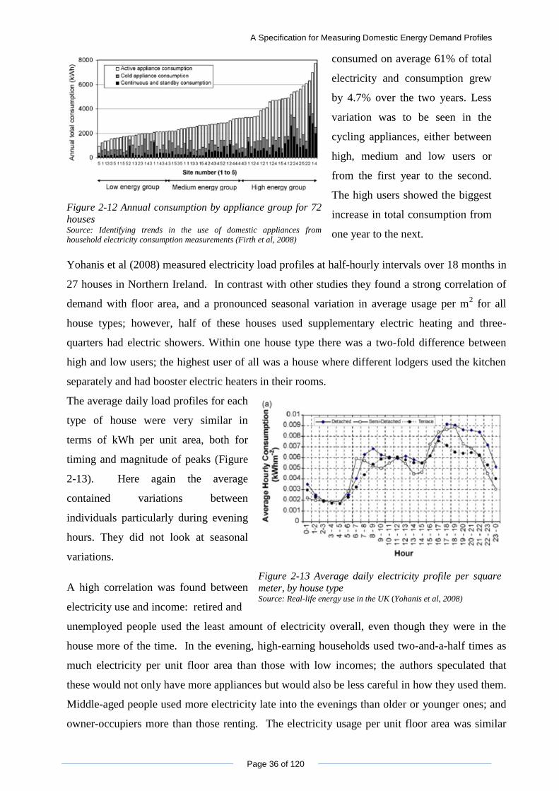
A Specification for Measuring Domestic Energy Demand Profiles
Page 36 of 120
Figure 2-12 Annual consumption by appliance group for 72
houses Source: Identifying trends in the use of domestic appliances from
household electricity consumption measurements (Firth et al, 2008)
consumed on average 61% of total
electricity and consumption grew
by 4.7% over the two years. Less
variation was to be seen in the
cycling appliances, either between
high, medium and low users or
from the first year to the second.
The high users showed the biggest
increase in total consumption from
one year to the next.
Yohanis et al (2008) measured electricity load profiles at half-hourly intervals over 18 months in
27 houses in Northern Ireland. In contrast with other studies they found a strong correlation of
demand with floor area, and a pronounced seasonal variation in average usage per m2 for all
house types; however, half of these houses used supplementary electric heating and three-
quarters had electric showers. Within one house type there was a two-fold difference between
high and low users; the highest user of all was a house where different lodgers used the kitchen
separately and had booster electric heaters in their rooms.
The average daily load profiles for each
type of house were very similar in
terms of kWh per unit area, both for
timing and magnitude of peaks (Figure
2-13). Here again the average
contained variations between
individuals particularly during evening
hours. They did not look at seasonal
variations.
A high correlation was found between
electricity use and income: retired and
Figure 2-13 Average daily electricity profile per square
meter, by house type Source: Real-life energy use in the UK (Yohanis et al, 2008)
unemployed people used the least amount of electricity overall, even though they were in the
house more of the time. In the evening, high-earning households used two-and-a-half times as
much electricity per unit floor area than those with low incomes; the authors speculated that
these would not only have more appliances but would also be less careful in how they used them.
Middle-aged people used more electricity late into the evenings than older or younger ones; and
owner-occupiers more than those renting. The electricity usage per unit floor area was similar
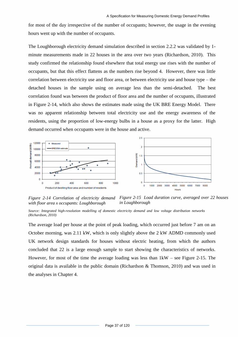
A Specification for Measuring Domestic Energy Demand Profiles
Page 37 of 120
for most of the day irrespective of the number of occupants; however, the usage in the evening
hours went up with the number of occupants.
The Loughborough electricity demand simulation described in section 2.2.2 was validated by 1-
minute measurements made in 22 houses in the area over two years (Richardson, 2010). This
study confirmed the relationship found elsewhere that total energy use rises with the number of
occupants, but that this effect flattens as the numbers rise beyond 4. However, there was little
correlation between electricity use and floor area, or between electricity use and house type – the
detached houses in the sample using on average less than the semi-detached. The best
correlation found was between the product of floor area and the number of occupants, illustrated
in Figure 2-14, which also shows the estimates made using the UK BRE Energy Model. There
was no apparent relationship between total electricity use and the energy awareness of the
residents, using the proportion of low-energy bulbs in a house as a proxy for the latter. High
demand occurred when occupants were in the house and active.
Figure 2-14 Correlation of electricity demand
with floor area x occupants: Loughborough
Figure 2-15 Load duration curve, averaged over 22 houses
in Loughborough
Source: Integrated high-resolution modelling of domestic electricity demand and low voltage distribution networks
(Richardson, 2010)
The average load per house at the point of peak loading, which occurred just before 7 am on an
October morning, was 2.11 kW, which is only slightly above the 2 kW ADMD commonly used
UK network design standards for houses without electric heating, from which the authors
concluded that 22 is a large enough sample to start showing the characteristics of networks.
However, for most of the time the average loading was less than 1kW – see Figure 2-15. The
original data is available in the public domain (Richardson & Thomson, 2010) and was used in
the analyses in Chapter 4.
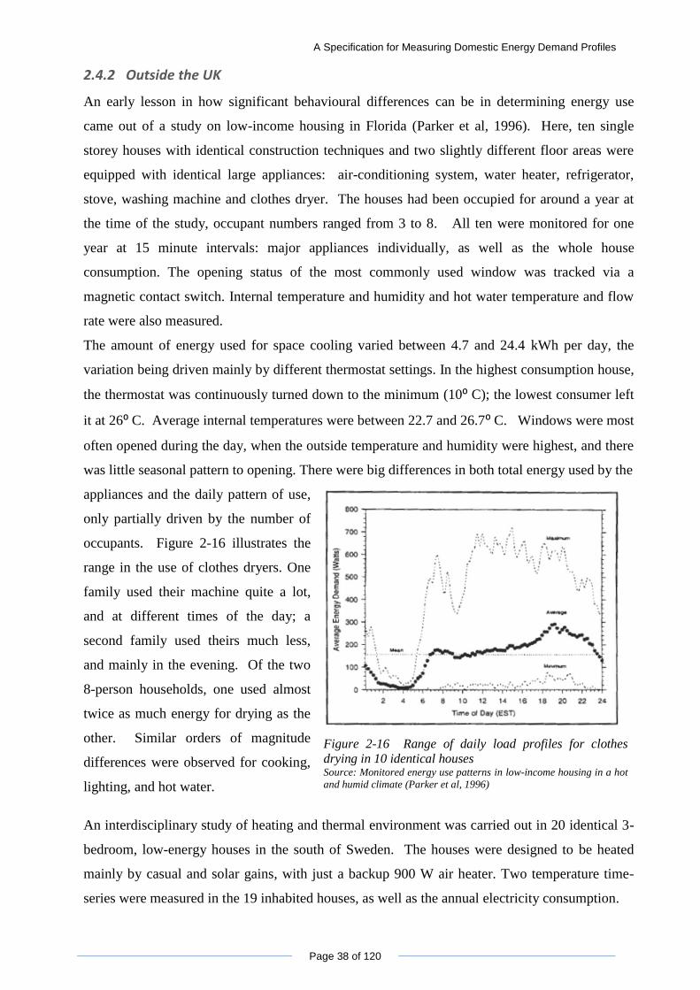
A Specification for Measuring Domestic Energy Demand Profiles
Page 38 of 120
2.4.2 Outside the UK
An early lesson in how significant behavioural differences can be in determining energy use
came out of a study on low-income housing in Florida (Parker et al, 1996). Here, ten single
storey houses with identical construction techniques and two slightly different floor areas were
equipped with identical large appliances: air-conditioning system, water heater, refrigerator,
stove, washing machine and clothes dryer. The houses had been occupied for around a year at
the time of the study, occupant numbers ranged from 3 to 8. All ten were monitored for one
year at 15 minute intervals: major appliances individually, as well as the whole house
consumption. The opening status of the most commonly used window was tracked via a
magnetic contact switch. Internal temperature and humidity and hot water temperature and flow
rate were also measured.
The amount of energy used for space cooling varied between 4.7 and 24.4 kWh per day, the
variation being driven mainly by different thermostat settings. In the highest consumption house,
the thermostat was continuously turned down to the minimum (10⁰ C); the lowest consumer left
it at 26⁰ C. Average internal temperatures were between 22.7 and 26.7⁰ C. Windows were most
often opened during the day, when the outside temperature and humidity were highest, and there
was little seasonal pattern to opening. There were big differences in both total energy used by the
appliances and the daily pattern of use,
only partially driven by the number of
occupants. Figure 2-16 illustrates the
range in the use of clothes dryers. One
family used their machine quite a lot,
and at different times of the day; a
second family used theirs much less,
and mainly in the evening. Of the two
8-person households, one used almost
twice as much energy for drying as the
other. Similar orders of magnitude
differences were observed for cooking,
lighting, and hot water.
Figure 2-16 Range of daily load profiles for clothes
drying in 10 identical houses Source: Monitored energy use patterns in low-income housing in a hot
and humid climate (Parker et al, 1996)
An interdisciplinary study of heating and thermal environment was carried out in 20 identical 3-
bedroom, low-energy houses in the south of Sweden. The houses were designed to be heated
mainly by casual and solar gains, with just a backup 900 W air heater. Two temperature time-
series were measured in the 19 inhabited houses, as well as the annual electricity consumption.
A Specification for Measuring Domestic Energy Demand Profiles
Page 39 of 120
In order to understand the heat transfer and air movement going on in the buildings, a detailed
set of readings was made in the one house which was empty – thermal mannequins were
introduced to simulate the presence of people. Temperatures were measured at 24 different
locations and heights. Air flow measurements were made in 4 locations, and an undisclosed
number of humidity measurements were also made. In addition, a series of semi-structured,
qualitative interviews lasting 1-2 hours was carried out with members of each household. There
was some divergence between measured indoor temperatures and the subjective view of
inhabitants who all found the houses to be colder than comfortable; on further investigation it
was concluded that this was because the air heaters were not in fact functioning as designed, and
were blowing a little air even when switched off (Isaakson & Karlsson, 2006). The published
report focuses on the interviews and contains little detail on the energy use measurements.
Measurements of climate, comfort and energy use in five low-energy, individually designed
houses in Australia were reported by Williamson (2010). Hourly readings of temperature and
relative humidity were made in the living areas and bedrooms. Outdoor temperature, wind
speed and solar radiation were measured, and energy and water consumption were taken from
bills. Interviews were carried out with the architects and with their clients who were in each case
the current occupants. These houses all used significantly less energy than equivalent houses in
that district, although according to the Australian method of assessment, all the buildings fell
below the current standard for energy efficient buildings. In fact, internal conditions fell outside
of the theoretically acceptable comfort limits much of the time. The occupants however said that
they were happy to live with a range of internal conditions that varied with the weather as this
made them feel „more connected to the environment‟.
A wider range of households was covered in a study of 4000 premises in central Finland where
hourly profiles were collected over a year (Räsänen et al, 2010). Here, only limited data was
available about each customer, chiefly the type of house or business, heating, and hot water and
cooking fuel. A two-stage, top-down analysis with neural networks was used to find the most
appropriate groupings whose members exhibited similar daily and seasonal profiles. Odd
combinations of user types emerged in some of the groupings: in one, 70% were households but
another 18% were customers describing themselves as commercial services, and a smaller
number of public sector, industrial and agricultural users. The worst-correlated cluster contained
a large proportion of holiday cottages and rental properties.
A 10-year study of household energy use (HEEP) was completed recently in New Zealand
(Isaacs et al, 2010). In this programme, 397 houses were monitored for a year each, with data
A Specification for Measuring Domestic Energy Demand Profiles
Page 40 of 120
collected at 10 minute intervals. Each type of energy use was measured, including output from
LPG heaters, open fires, and solid fuel burners – a method of estimating the output of the latter
was developed during the course of the survey. Temperatures were measured in living- and
bedrooms. Hot water consumption was measured separately, and over 13,800 individual
electrical appliances were monitored over the course of the study. Each house was surveyed at
the start of the collection programme, and socio-economic data were collected. The final report
gives information on practical experiences with various types of instrumentation and issues faced
in collecting data: for example, one third of the thermostats on hot water cylinders were found to
be inaccurate to more than +/-10⁰C, and one in every 6 refrigerators turned out to be faulty – this
could be seen in the extended on-cycles they measured.
New Zealanders apparently also have only a vague understanding of how they actually use
heating: when asked about how long they heated their houses, responses indicated over a month
less than the measured heating season. The warmest houses were those with solid fuel burners
because it was difficult to control their heat output. The average evening temperature in the
living rooms was 17.9⁰ C in the winter and 23.1⁰ C in summer, implying that New Zealanders
are more willing to live with seasonal variation than their UK or US counterparts. Newly built
houses were warmer than older ones both in summer and winter: various possible reasons were
suggested such as increased insulation, better draught-proofing or higher levels of glazing
relative to floor area, but these did not account for the difference. In the end the authors
suggested that occupant behaviour must be responsible.
The authors were not able to identify correlations with survey data that would explain
differences in energy use. Income level was found to explain less than 2% of the variation in
domestic hot water or appliance use, and not to be correlated at all with heating energy.
Household size drove a quarter of the variation in hot water use, and 9% of other use, but was
not correlated to heating either. A combination of income level, household size and life stage of
the family were found to explain only about a quarter of the variation in overall energy use. The
top 20% of households used 38% of the total hot water.
Baseload power (standby plus cycling appliances) was the equivalent of 112 W continuously for
all houses. Although it formed only 10% of the energy used, baseload had a large impact on the
total network as it contains a significant reactive power component from refrigerator motors and
small transformers – measured power factors were in the range 0.5-0.7. The report provides a
table of average measured standby power and energy use of a long list of common appliances.
A Specification for Measuring Domestic Energy Demand Profiles
Page 41 of 120
A similar, detailed national survey was carried out on 400 houses in Sweden, although covering
electricity consumption only (Zimmermann, 2009). The focus was on understanding end-use, so
in addition to measuring total consumption at 10-minute intervals, up to 15 power meters were
used per house on high-power circuits and individual appliances. Another 16-20 lower power
appliances per house were measured with serial watt meters, and 25 „lamp-meters‟ were used to
record the profiles of lights switching on and off. Internal and external temperatures were also
measured. Results for houses and flats were presented separately and sorted by age group of
inhabitants and the family type (single person, couple, or family with children).
Households of the same age and family type showed a wide variation in energy use, whether
expressed as a total, by unit floor area or by person, although those which had electric heating
showed a smaller range in annual use per unit area. Older people used slightly less electricity
than younger ones. The largest energy users, and those responsible for the highest peak loads,
were couples of working age without children – probably an indicator that disposable income is
more important than age as such. Baseload power averaged 87 W across all the houses and flats,
but around 5% used 0.5 kW or more.
The daily load curves for refrigerators showed about 25% difference between the peak
consumption in the early evenings – when food preparation might be expected to be happening,
with the fridge being opened frequently – and the lowest level in the early morning. A small
seasonal effect was also apparent. Freezers showed much less variability. Washing machine
consumption was reasonably constant at 60-70 kWh/person per year, reducing only for families
of 5 or more. Energy use in clothes drying and in dishwashing did not show such a trend,
although more is used per person in apartments than in houses where there might be more space
for drying indoors or drying clothes outside. There was a strong seasonal effect in cooking, with
40% more energy used in an average midwinter week than in summer. Most of the energy used
in cooking went to the hob and oven. The annual consumption per person reduced slightly with
household size up to 3, but after that it was constant at around 110 kWh per person per year.
There was greater variation in the actual use of energy for lighting than in the installed wattage
of light fittings in houses. 50% more energy was consumed for lighting in the middle of the
winter than in the summer. A smaller seasonal variation was observed for televisions and other
consumer electronics. There was a very large variability in hot water use per person. Air dryers,
water beds and aquaria were found to consume significant energy in some houses.
Data on energy used for lighting in 69 of these Swedish households was analysed further by
Bladh & Krantz (2008). They tested two hypotheses: first that lighting use per person goes down
if there are more people in the house sharing the same lights. This turned out to be true, but the
A Specification for Measuring Domestic Energy Demand Profiles
Page 42 of 120
effect was significant mainly when moving from 1 to 2 persons in the household, but beyond that
the reduction is smaller than the variation in individual households of the same size. The second
hypothesis was that older people are less profligate in their use of lighting than younger ones.
Although the older households did use less energy than the younger age groups, the sample was
not large enough to draw conclusions about whether it was age as such or different generational
expectations that accounted for the difference.
The authors also conducted detailed interviews with 7 of the households, including a ‟lamp-tour‟
of each house, during which the occupants explained how and when each light source was used.
They found very different levels and patterns of usage even between households of the same
size, depending on how much they were home and to some extent on income. However, each
house showed a consistent pattern, especially on weekdays. Most explained their use of lighting
in terms of cosiness and atmosphere rather than utility – lights were left on in dark spaces most
of the day, or were operated with timers to provide a welcoming feeling when coming home. All
the houses had many light fittings that were not used regularly, and in some cases not used at all
- no household used more than a quarter of the total installed wattage of lamps. The authors also
incidentally discovered that even though an average of 25 lamps had been monitored in each
house, the study had failed to pick up some of the most frequently used ones.
A monitoring campaign on electricity use by appliance and end-use was carried out in 12
European countries in 2006-08 (REMODECE, 2008). Measurements were made at 10-minute
intervals in around 100 houses per country, with overall consumption and that of various
appliances monitored, and an extensive survey of households and household behaviours carried
out. Around 2 weeks‟ worth of data was collected at each house, and this was extrapolated to
give annual demand and hourly average daily demand profiles by end use; given the seasonal
variation observed in longer-term studies, this is a limitation in quality. The most interesting
outcome from this programme for the present study lies in the differences seen between
countries in how electricity and appliances are used.
2.5 Influence of social attitudes and habits
Occupants‟ attitudes and habits appear to be very important, causing large variation in energy
use between two apparently similar families living in similar circumstances. This section
reviews lessons from some relevant studies.
A Specification for Measuring Domestic Energy Demand Profiles
Page 43 of 120
In the UK, BRE‟s regular fact file on domestic energy shows how general expectations on
comfort levels have increased over time. Average winter temperature in houses has risen from
around 12⁰C in 1970 to 18⁰C by 2008, because the spread of central heating has allowed the
whole house to be heated evenly. The authors expect that this trend may plateau at 19-20⁰C,
although they warn that German experience with passive houses is that people are now looking
for a mean internal temperature of 22⁰C (Shorrock & Utley, 2008).
Prescriptive temperature and humidity standards in offices have accustomed people working in
closely conditioned buildings to expect little seasonal variation. However, a range of studies
reviewed by Roaf et al (2010) shows that a much wider range of temperatures can feel perfectly
comfortable, provided that changes are gradual and that people are dressed appropriately. An
extreme example quoted is the government sponsored „Cool Biz‟ programme in Japan, where
gradual social conditioning permitted workers to wear loose, informal clothes to work and
therefore allowed public buildings to operate without air-conditioning at temperatures up to 28⁰C
without the people in them feeling uncomfortable.
A government sponsored report describes how changing social patterns have a big impact on
energy use – if teenage children using computers and TVs in their bedrooms, not only are there
more appliances but more rooms have to be heated and lit. If families eat home-cooked meals
together, more energy is used, and in a narrower time period, than if individuals microwave
ready-made meals for themselves at different times. New mobile consumer electronic products
are constantly introduced, and now become widespread within a matter months. Microwaves,
TVs and mobile gadgets use standby power, so more of these appliances results in more baseload
power consumed. Low energy light bulbs are becoming more acceptable to consumers, but
fashions for more, and brighter light fittings can counter the savings (Owen, 2006).
Technology developments appear to offer increasing numbers of ways for people to consume
more energy, but their actual effect depends how quickly appliances become a „must-have‟ item.
Until recently, consumer products were not considered to be a major user of energy; however
when plasma televisions were introduced they were marketed as not only a more stylish product,
but also one that could replace many others such as radios and computer screens. Households
replacing a cathode ray set with plasma are thus using not only four times as much electricity
when watching TV, but forty times as much when listening to the radio; and some even use them
as replacements for pictures (Crosbie, 2008). In an attempt to understand how products could
be designed so as to minimise consumption in use, Tang & Bhamra (2008) recorded interviews
with customers and observations of refrigerators and freezers being used in homes. They
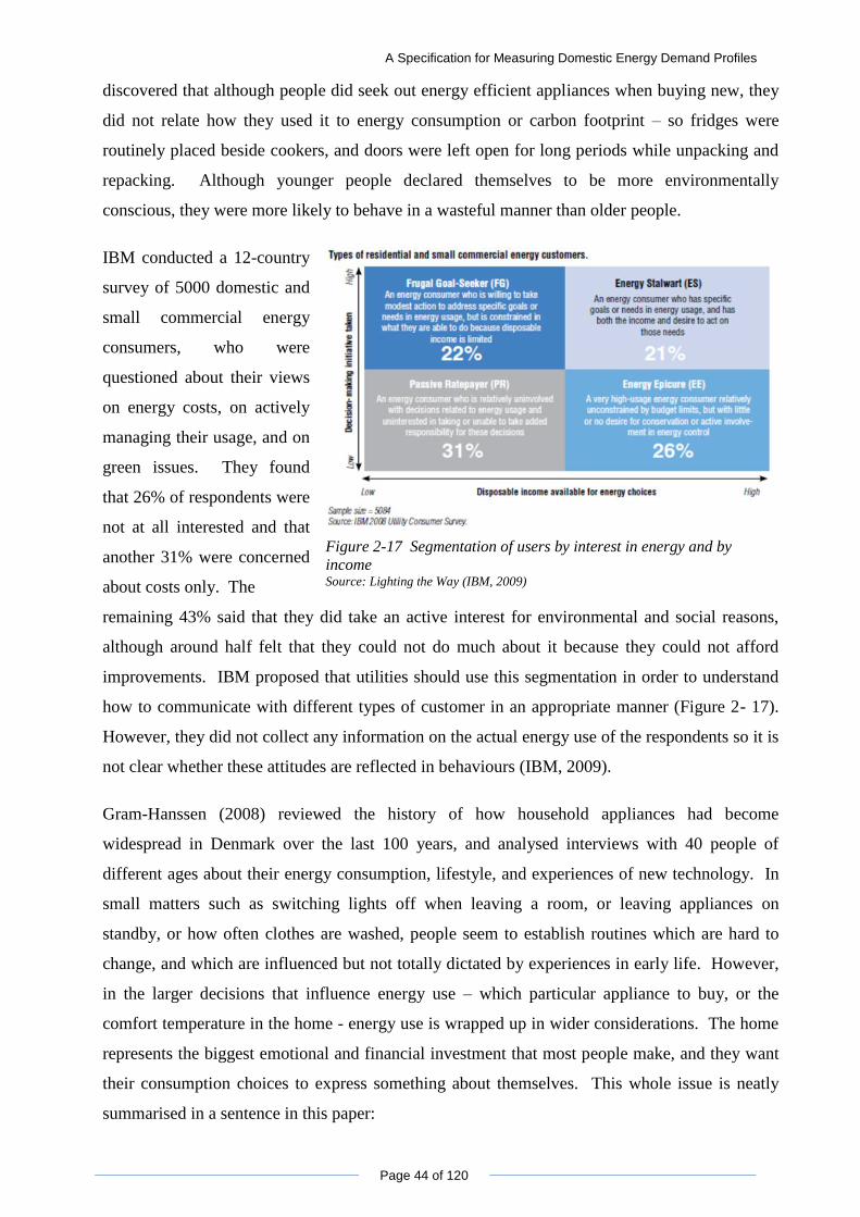
A Specification for Measuring Domestic Energy Demand Profiles
Page 44 of 120
discovered that although people did seek out energy efficient appliances when buying new, they
did not relate how they used it to energy consumption or carbon footprint – so fridges were
routinely placed beside cookers, and doors were left open for long periods while unpacking and
repacking. Although younger people declared themselves to be more environmentally
conscious, they were more likely to behave in a wasteful manner than older people.
IBM conducted a 12-country
survey of 5000 domestic and
small commercial energy
consumers, who were
questioned about their views
on energy costs, on actively
managing their usage, and on
green issues. They found
that 26% of respondents were
not at all interested and that
another 31% were concerned
about costs only. The
Figure 2-17 Segmentation of users by interest in energy and by
income Source: Lighting the Way (IBM, 2009)
remaining 43% said that they did take an active interest for environmental and social reasons,
although around half felt that they could not do much about it because they could not afford
improvements. IBM proposed that utilities should use this segmentation in order to understand
how to communicate with different types of customer in an appropriate manner (Figure 2- 17).
However, they did not collect any information on the actual energy use of the respondents so it is
not clear whether these attitudes are reflected in behaviours (IBM, 2009).
Gram-Hanssen (2008) reviewed the history of how household appliances had become
widespread in Denmark over the last 100 years, and analysed interviews with 40 people of
different ages about their energy consumption, lifestyle, and experiences of new technology. In
small matters such as switching lights off when leaving a room, or leaving appliances on
standby, or how often clothes are washed, people seem to establish routines which are hard to
change, and which are influenced but not totally dictated by experiences in early life. However,
in the larger decisions that influence energy use – which particular appliance to buy, or the
comfort temperature in the home - energy use is wrapped up in wider considerations. The home
represents the biggest emotional and financial investment that most people make, and they want
their consumption choices to express something about themselves. This whole issue is neatly
summarised in a sentence in this paper:

A Specification for Measuring Domestic Energy Demand Profiles
Page 45 of 120
“The answer to the question of whether campaigns to keep low indoor temperatures have influenced the temperature level is that those who prefer to have a lower temperature also use energy consumption as an argument” (Gram-Hanssen, 2008)
A Specification for Measuring Domestic Energy Demand Profiles
Page 46 of 120
3 Lessons from demand profiling
This chapter presents a systematic review of the key lessons from the literature surveyed in
Chapter 2 as regards energy demand profiling. A tabular comparison of the measurement
programmes outlines in Section 2.4 is included in Appendix 2.
3.1 Data availability
Measured data on energy demand profiles is hard to find. In the UK, utility companies keep
their data confidential for commercial and data privacy reasons, and have not always been able
to retrieve it when needed (Boehme et al, 2006). Electricity profiles produced by the Load
Research Association in the late 1990s have been used by others (Yao & Steemers 2005; Born et
al 2001b; Stokes et al 2004). However, only the original national average profiles by customer
class proved easily retrievable by the present author – the source for the detailed lighting data
cited by Stokes et al (2004) for example could no longer be found. Elexon does make its annual
regression coefficients available for purchase, and from these it would be possible to reconstruct
updated, regional average electricity profiles for each year, but the original data is not kept. No
equivalent data is available from National Grid on gas profiles (J Ryder, XOServe, personal
communication, 22 August 2011). The EDRP programme does promise that its half-hourly gas
and electricity data will eventually be made available to researchers, but a request for access to
this is still on the waiting list.
Outside the UK, data from the Swedish Energy Agency measurement programme were made
available to Widen et al (2010) for model calibration, and are said to be accessible to other
researchers, as in the data from the HEEP programme in New Zealand (Isaacs et al, 2010). The
REMODECE (2008) data are accessible via the internet, but only at the level of hourly averaged
profiles for the end uses measured.
In some cases, data collected by one research group has apparently been used by others, but little
information is given: Jenkins et al (2009) cite Newborough & Augood (1999) as the source of
demand profiles they used, although this data were not actually published in the original paper;
Hawkes & Leach (2005) used electricity demand measured by BRE for a different project.
Most commonly, researchers have collected their own data when needed. Because their focus is
on the application, they do not always fully report what was measured and how. Examples are:
the number of hot water tanks monitored by Lane & Beute (1996), the specific CHP data items
measured by Bakker et al (2008), the electricity and hot water measurements in Korean
apartments by Clarke at al (2005), the heating demand profile in Hawkes & Leach (2005).
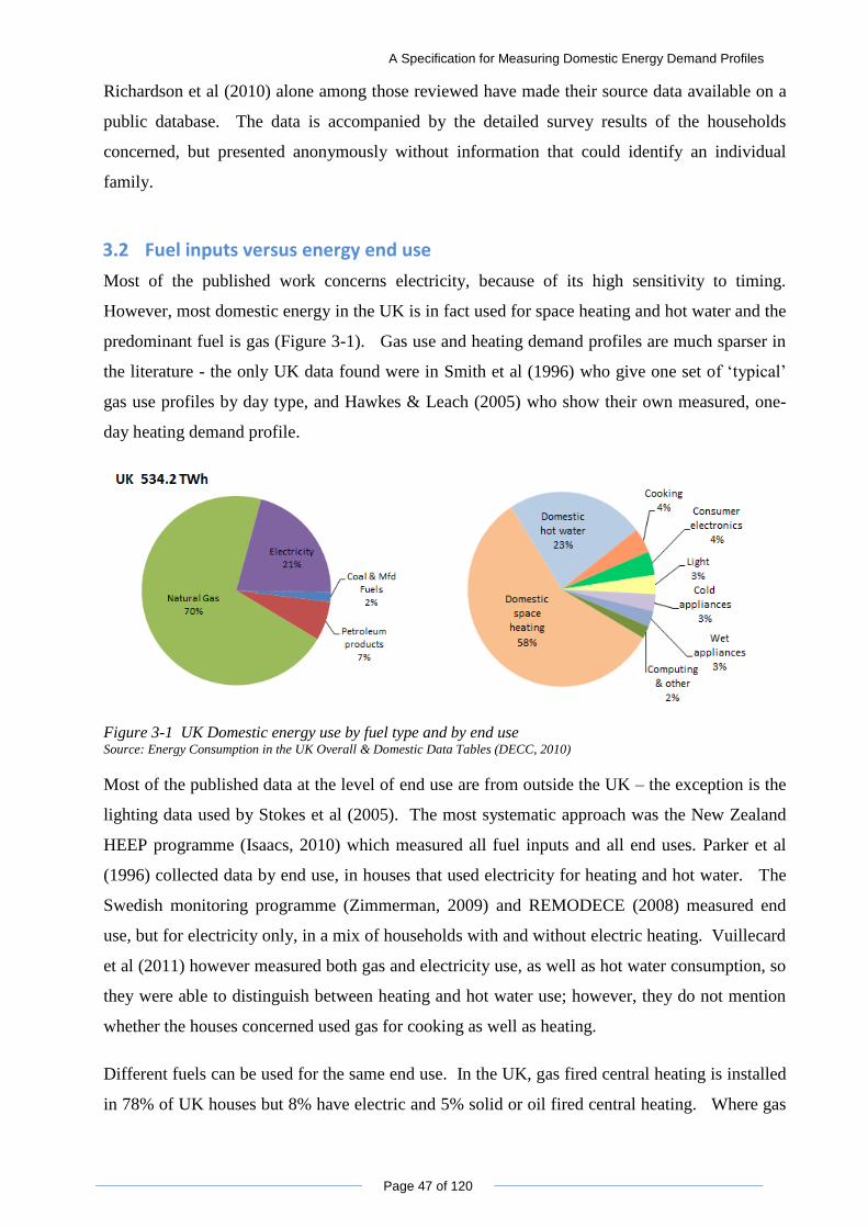
A Specification for Measuring Domestic Energy Demand Profiles
Page 47 of 120
Richardson et al (2010) alone among those reviewed have made their source data available on a
public database. The data is accompanied by the detailed survey results of the households
concerned, but presented anonymously without information that could identify an individual
family.
3.2 Fuel inputs versus energy end use
Most of the published work concerns electricity, because of its high sensitivity to timing.
However, most domestic energy in the UK is in fact used for space heating and hot water and the
predominant fuel is gas (Figure 3-1). Gas use and heating demand profiles are much sparser in
the literature - the only UK data found were in Smith et al (1996) who give one set of „typical‟
gas use profiles by day type, and Hawkes & Leach (2005) who show their own measured, one-
day heating demand profile.
Figure 3-1 UK Domestic energy use by fuel type and by end use Source: Energy Consumption in the UK Overall & Domestic Data Tables (DECC, 2010)
Most of the published data at the level of end use are from outside the UK – the exception is the
lighting data used by Stokes et al (2005). The most systematic approach was the New Zealand
HEEP programme (Isaacs, 2010) which measured all fuel inputs and all end uses. Parker et al
(1996) collected data by end use, in houses that used electricity for heating and hot water. The
Swedish monitoring programme (Zimmerman, 2009) and REMODECE (2008) measured end
use, but for electricity only, in a mix of households with and without electric heating. Vuillecard
et al (2011) however measured both gas and electricity use, as well as hot water consumption, so
they were able to distinguish between heating and hot water use; however, they do not mention
whether the houses concerned used gas for cooking as well as heating.
Different fuels can be used for the same end use. In the UK, gas fired central heating is installed
in 78% of UK houses but 8% have electric and 5% solid or oil fired central heating. Where gas
A Specification for Measuring Domestic Energy Demand Profiles
Page 48 of 120
is available it is often used for cooking as well as fuelling the heating and hot water system; but
electricity accounts for 15% of domestic hot water and around 50% of cooking demand (DECC,
2010). If only fuel inputs are measured, these differences can confuse the interpretation of
differences - an example is in Yohanis et al (2008) where houses with and without electric
heating are analysed as a single sample.
Another set of end-uses that it is important to distinguish separately is those whose timing could
potentially be shifted away from peak load period. Wet appliances are one category (Strbac, et
al., 2010), but hot water storage has also been investigated (Lane & Beute, 1996) and well as
heating (Hong et al, 2011) - electric storage heaters are a familiar technology that could be
brought up to date as a smart appliance. Cold appliances are being introduced which are capable
of using grid frequency changes to guide switching off for a short period to ease peak loading.
Lighting, consumer electronics and other miscellaneous appliances all use electricity only, and it
is unlikely to be acceptable to consumers to attempt to shift the time when they are on.
However, both lighting and consumer electronics are areas where technology changes are
happening: in the case of lighting, technology is encouraging lower energy use - low energy
bulbs and fittings now constitute nearly a quarter of all lighting appliances – while in the case of
consumer electronics the drive is in the other direction (Owens, 2006).
3.3 What the sample represents
3.3.1 Size and composition
The ideal method of selecting properties to measure would be to choose a random sample which
includes appropriate proportions of high, medium and low energy users as well as types of
property and household in the area (Schrock, 1997). However, this is rarely possible as it
requires access to meter readings from all the suppliers in the area; it has been used only in large
national data gathering programmes (Elexon, 2011; Isaacs, et al, 2010; Zimmermann, 2009).
Much of the published work on demand measurement relates to one locality and a limited
number of households. In some cases, this is because the project set out to investigate low-
energy or affordable housing (Isaakson & Karlsson, 2006; Gill et al, 2011; Parker et al, 1996;
Summerfield et al, 2010) or test new energy systems (Firth et al, 2009), and here the samples
were predefined. Some researchers whose primary concern was to generate data for
investigating technologies without too much concern about how representative this might be,
limited themselves to eight, four (Olofsson et al, 1998; Bakker et al, 2008) or even one (Yao &
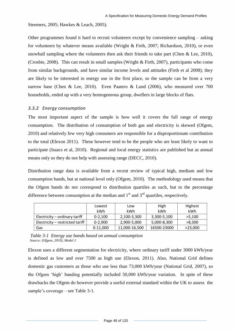
A Specification for Measuring Domestic Energy Demand Profiles
Page 49 of 120
Steemers, 2005; Hawkes & Leach, 2005).
Other programmes found it hard to recruit volunteers except by convenience sampling – asking
for volunteers by whatever means available (Wright & Firth, 2007; Richardson, 2010), or even
snowball sampling where the volunteers then ask their friends to take part (Chen & Lee, 2010),
(Crosbie, 2008). This can result in small samples (Wright & Firth, 2007), participants who come
from similar backgrounds, and have similar income levels and attitudes (Firth et al 2008); they
are likely to be interested in energy use in the first place, so the sample can be from a very
narrow base (Chen & Lee, 2010). Even Paatero & Lund (2006), who measured over 700
households, ended up with a very homogeneous group, dwellers in large blocks of flats.
3.3.2 Energy consumption
The most important aspect of the sample is how well it covers the full range of energy
consumption. The distribution of consumption of both gas and electricity is skewed (Ofgem,
2010) and relatively few very high consumers are responsible for a disproportionate contribution
to the total (Elexon 2011). These however tend to be the people who are least likely to want to
participate (Isaacs et al, 2010). Regional and local energy statistics are published but as annual
means only so they do not help with assessing range (DECC, 2010).
Distribution range data is available from a recent review of typical high, medium and low
consumption bands, but at national level only (Ofgem, 2010). The methodology used means that
the Ofgem bands do not correspond to distribution quartiles as such, but to the percentage
difference between consumption at the median and 1st and 3
rd quartiles, respectively.
Lowest kWh
Low kWh
High kWh
Highest kWh
Electricity – ordinary tariff 0-2,100 2,100-3,300 3,300-5,100 >5,100
Electricity – restricted tariff 0-2,900 2,900-5,000 5,000-8,300 >8,300
Gas 0-11,000 11,000-16,500 16500-23000 >23,000
Table 3-1 Energy use bands based on annual consumption Source: (Ofgem, 2010), Model 2
Elexon uses a different segmentation for electricity, where ordinary tariff under 3000 kWh/year
is defined as low and over 7500 as high use (Elexon, 2011). Also, National Grid defines
domestic gas customers as those who use less than 73,000 kWh/year (National Grid, 2007), so
the Ofgem „high‟ banding potentially included 50,000 kWh/year variation. In spite of these
drawbacks the Ofgem do however provide a useful external standard within the UK to assess the
sample‟s coverage – see Table 3-1.
A Specification for Measuring Domestic Energy Demand Profiles
Page 50 of 120
3.3.3 Other context
Many measurement programmes restrict themselves to looking at energy use, without caring too
much about the context (Elexon, 2011; Wright & Firth, 2007; Räsänen et al, 2010) However, to
understand what drives consumption, information is needed about the households concerned.
Various kinds of data have been collected, often different for each programme – Appendix 2 lists
the variants. Housing type and number of occupants is the most consistently reported.
Appliance ownership is also often used, although this can be at a high level only (Yohanis et al,
2008; Richardson, 2010) or a full appliance audit (Isaacs et al, 2010). Household income data
was collected by Summerfield et al (2007), Yohanis et al (2010), and Isaacs et al (2010); age
and/or life stage of occupants was also recorded by these and by Zimmermann (2009).
Statistics on housing type at local level are available from Department of Commerce & Local
Government (Dept. Comm & Local Govt, 2011) or the Scottish Government (2009). Household
size, and disposable income bands, are published at national level in the annual Social Trends
report (ONS, 2009). Annual statistics on ownership of appliances are also published (DECC,
2010).
A potentially illuminating context category would be attitude to energy use. One model for this
is provided by the four-sector segmentation used by IBM (2009), which is based on structured
interview questions on income level and interest in matters to do with energy. Richardson
(2010) tried without apparent success to use the number of low-energy light bulbs in a household
as a proxy for energy-consciousness. However, the findings of Tang & Bhamra (2008) and
Bladh & Krantz (2008) suggest that awareness of energy and environmental issues does not
necessarily translate into low-energy behaviours. The survey used by REMODECE (2008)
includes questions on specific behavioural aspects of appliance use.
Interviews appear to give a better understanding of the context of the measurements than simple
questionnaires (Isaakson & Karlsson, 2006; Williamson, 2010). The best results are obtained
from structured but not closed questions. Training the interviewers beforehand, and using the
same people for all the interviews, gives consistency in interpreting and recording answers
(Crosbie, 2008).
3.4 Data collection
3.4.1 Frequency
There is a wide range in the frequency of data profile measurements, ranging from hourly to 1-
A Specification for Measuring Domestic Energy Demand Profiles
Page 51 of 120
minute frequency, detailed in Appendix 2. For electricity measurements, a 1-minute resolution
was found best to capture the peaks and short duration events (Newborough & Augood, 1999;
Richardson et al, 2009). Firth et al (2009) argue that 5 minutes makes it easier to store longer
data sets without losing too much detail; and indeed one of the problems experienced by
Richardson (2010) with 1-minute data was the limited storage capacity of the data loggers.
Longer than 5 minutes can give false estimates when looking at the behaviour of new
technologies: average demand and average supply from a PV system may balance over half an
hour but this can mask large fluctuations with a high-short term demand on the grid followed by
a short period of export (Wright & Firth, 2007).
Less discussion is available around gas and heat flow measurement frequency. Hawkes & Leach
(2005) showed that 10 minutes is the longest time step that gives good data for sizing CHP
systems; the gas smart meter use cases ask for 6 minutes (ENA, 2010). Room temperature and
humidity do not vary as fast; 15 minutes was the shortest frequency for these (Parker et al, 1996).
Vuillecard et al (2011) report measuring both gas use and hot water flow at 1-minute intervals as
well as electricity and even their temperature measurements may have been at that resolution.
3.4.2 Duration
Most data collection has been run for between one and two years (Appendix 2), to ensure that
high heating consumption in winter or high cooling in summer is covered adequately, and
seasonal fluctuations become apparent. However, Newborough & Augood (1999) restricted
their electricity measurements to 1 month, and Wright & Firth‟s electricity profiles (2007)
missed out an autumn. In the Swedish study only 10% of households were measured over a full
year, the rest for one month only, and REMODECE (2008) generally managed only 2 weeks for
each household – although they originally set out to cover twice that period. Hot water demand
was also measured over shorter periods - three months (Chen & Lee, 2010; Gill et al, 2011), or
even just 14 days (Lane & Beute, 1996) - on the assumption that this will not vary much.
Experience from various programmes (Gill et al, 2011; Isaacs, et al, 2010) suggests that adequate
results can be obtained from a data collection plan which covers some of the sample properties in
detail, and the rest at a reduced level, as long as a whole winter is included in each case.
3.4.3 Immediacy
Most programmes have logged data on site, and retrieved it periodically at a later date. Elexon
(2011) is the most extreme, collecting the loggers and analysing the data only after the end of a
full year. In both the Swedish and the New Zealand programmes, data was logged in each house
A Specification for Measuring Domestic Energy Demand Profiles
Page 52 of 120
for a month before being downloaded during visits by a dedicated collection team
(Zimmermann, 2009; Isaacs et al, 2010). Firth et al (2008) were able to download remotely
using the public telephone system and Richardson (2010) and Yohanis et al (2008) also used
dial-up modems, but in both cases this was done only at intervals of several weeks, by which
time it was difficult to investigate anomalous data. The DATA BIRD automatic meter reading
system in Leicester has a one-day turnaround, using a network of radio repeating stations
through the city to collect low-power transmission from local data loggers and forward them to a
central receiver; from here they are downloaded daily to the analysis system (Ferreira, 2009).
3.4.4 Consistency and accuracy
The instrumentation used in measurements is not always reported, but where this is, overall
electricity demand profiles were measured with a power meter close to and at the same level of
accuracy as the utility meter (Richardson 2010; Isaacs et al, 2010). Accuracy standards for
meters vary by country but in the UK this is +2.5%/-3.5% (Ofgem, 2005).
For heating, the common approach is to measure temperature profiles in living rooms and at least
one bedroom, and fuel consumption only periodically (Isaakson & Karlsson, 2006; Summerfield
et al, 2007; Williamson, 2005;). Where instrumentation was mentioned, the temperature sensors
were rated at +/0.5 ⁰C accuracy (Shipworth, et al. 2010). Heat flow was measured by Gill et al,
(2011), in the context of a district heating system where hot water is metered by the utility
company. Vuillecard et al (2011) alone reported measuring heat flow into the heating system,
separately from hot water consumption.
Where end-use or individual appliances were measured, different approaches were used.
REMODECE‟s methodology gives two different lists of priority items, both individual
appliances and groups; however, dishwashers or cooking are not in either priority list; and it is
not clear from the database how well the methodology was followed in each individual country.
HEEP looked at end-use in a quarter of their sample houses. They measured power at circuit
level for electric heating, hot water and cooking to the same standard as overall electricity
consumption. However, for individual appliances they deployed only 2-3 transponders per
house, using a random selection procedure each month to decide which to monitor; this meant
that some of the time they were monitoring equipment that was hardly used (Isaacs et al, 2010).
The Swedish programme took the most systematic approach, monitoring 30 circuits and
appliances plus 25 lamps in each house (Zimmermann, 2009). However, even they did not
always manage to measure the right things: the follow up interviews by Bladh & Krantz (2008)
in seven houses showed that some of the most frequently used lights had been missed.
A Specification for Measuring Domestic Energy Demand Profiles
Page 53 of 120
3.5 Practical issues
3.5.1 Finding volunteers
This is the first major problem encountered by all measurement programmes. These can be
perceived as intrusive, and as passing judgement on lifestyle and consumer choice (Ofverholm,
2009). Those who volunteer are almost always people who are interested in energy use in the
first place, so the sample can be from a very narrow base (Chen & Lee, 2010; Firth et al, 2008).
Some kind of incentive for participation helps (Elexon, 2011; Richardson, 2010),
3.5.2 Data privacy
Data privacy / security considerations must be planned for carefully. For example, at
Strathclyde, such an exercise would fall into the University Ethics Committee‟s definition of
“a situation where highly personal, intimate or other private or confidential information of a personal
nature is sought” (University of Strathclyde, 2009)
for which approval must be sought from either the University or Departmental Ethics
Committee. Their guidelines specify how volunteers may be recruited, and require assuring
participant anonymity and security of any personal information collected – in this case, addresses
and meter numbers. There may be a need to register the database with the Information
Commissioners‟ Office, under the Data Protection Act. If data is being transmitted from the
volunteer house via modem or internet, security during transmission will be an issue, as load
profiles alone contain a lot of information about when people are in or out of the house during
the day (Richardson, 2010).
3.5.3 Access and equipment location
Access to premises to install equipment may be an issue especially if people are out during the
day – this was a problem reported by all four utilities participating in EDRP (Ofgem, 2010).
Other recurring problems reported are whether there is space to install a second meter on the
existing meter box (Isaacs, et al., 2010), (Richardson, 2010).
3.5.4 Data transmission and storage
Collecting, cleansing and handling such large amounts of data are a big challenge in any
collection programme. Wright & Firth (2007) found that their transmissions dropped out
periodically, and when they resumed the transmission for next period started with spikes that
accumulated all the data missed previously. Richardson (2010) lost data because the modems
could break down and transmission was sensitive to interference, even a car parked in the wrong
place could cause drop-out.
A Specification for Measuring Domestic Energy Demand Profiles
Page 54 of 120
The rapid growth of computing power does mean that tasks that were too large to handle a few
years ago can be carried out easily today. In 2008, Richardson (2010) needed to use a Microsoft
Server SQL database to handle one year‟s worth of 1-minute data. Three years on, it has been
possible to analyse those 500,000 lines of data per house, including graphing, on a normal laptop
using Excel.
3.5.5 Cost and effort considerations
Instrumentation costs have been one of the barriers in reported measurement programmes.
(Schrock, 1997) reported that orders of magnitude at that time were:
Run-time meter with 1-4 channel logger: $100-200
Multi-channel data loggers: $800-$4000
3-phase power analyser: $3,000-15,000
The HEEP project (Isaacs, et al., 2010) found it cheaper to build their own loggers than buy them
- building 750 temperature a dozen 16-channel electricity loggers. However, a cursory Internet
search showed that sensors and loggers are now available for the consumer market at relatively
low prices. A ThermaData combined temperature and RH logger, with an accuracy of +/-0.5% T
and +/-2% RH that will record 75 days‟ worth of 15 min readings can be bought for around £90.
A home electricity monitor such as the Current Cost meter marketed by Envi which is capable of
measuring up to 10 channels of current only, costs under £100 including sensors.
The effort involved in installing, testing, downloading data and checking for data quality is high.
One and a half days out of every 3 weeks was required for data download and checking for the
22 meters in Loughborough (Richardson, 2010) HEEP reported 800 person days to install
monitoring equipment in 400 houses (including travelling time) and employed 12 full-time
download field staff (Isaacs, et al., 2010). The Swedish study had a similar level of costs for
analysis and reporting as for equipment and installation (Ofverholm, 2009).
3.6 Consistency in outcomes
3.6.1 Energy use
Peak loads measured over 1 minute for one month by Newborough & Augood (1999) were 4-7
kW if no space heating used, and up to 15kW where it was (N&A); Wright & Firth (2007) found
8-9 kW peak loads, measuring average load over 1 minute for 9 months. Both also found similar
weekly load factors, 0.06-0.15 in the first instance and 0.08-0.15 in the second. The Swedish
study reported 3-16 kW with, and 3-16 kW peak loads without electric heating (Zimmermann,
A Specification for Measuring Domestic Energy Demand Profiles
Page 55 of 120
2009), but this may in reality be higher because the load was averaged over 10 minutes. The
average power over the year reported in UK measurements was consistently under1 kW per
household (Newborough & Augood, 1999; Wright & Firth, 2007; Richardson et al, 2010; Gill et
al, 2011, Yohanis et al, 2007). This was also largely true in New Zealand, except in the far
South where more electric heating is used (Isaacs et al, 2010). In Florida, the average in the low-
income houses surveyed was around 1kW, excluding air conditioning and air handling (Parker et
al, 1996). Sweden alone has reported significantly higher overall power usage – for homes
without electric heating, the lowest user band averaged 1.7 and the highest 4.7 kW, - the lower
values applied to flats and to smaller families (Zimmermann, 2009).
3.6.2 Correlations
Some work has assumed that only heating and lighting is subject to seasonal variation and that
most appliances or hot water demand can be treated as constant (Lane & Beute, 1996;
Newborough & Augood, 1999; Yao & Steemers, 2005 REMODECE, 2008). However, the
Swedish measurement programme which looked in detail at end-uses showed significant
seasonal variation in several end-uses: refrigeration, cooking, consumer appliances
(Zimmermann, 2009).
Yohanis et al (2008) whose sample included a large proportion of houses with electric heating
found that electricity use is well correlated with floor area, however, others such as Gill et al
(2011) or Summerfield et al (2010), whose sample houses used other forms of heating did not.
Floor area is a driver of energy used for space heating (Summerfield et al, 2010). Occupancy
pattern (Richardson 2010) and to a lesser extent occupant numbers are the main drivers of other
end-uses, although the effect of increasing occupant numbers levels off as more are added
(Zimmerman 2009); indeed, the biggest difference is seen between single and two-person
dwellings (Bladh & Krantz, 2008).
Income and energy use were found to be well correlated by Yohanis et al (2008), and by
inference also by Summerfield et al (2007) who found that the higher energy consumers in the
first survey were the ones that had built extensions onto their houses, and Zimmerman (2009)
who found that two-adult households consumed more electricity than families in similar
properties, presumably because of higher disposable income.
Observed trends in energy use with time are ambiguous, partly because the data sets are very
few. Firth et al (2007) found that although the average energy use in their 72-house sample had
increased by 4.5% from one year to the next, this increase was mainly in the sub-group that were
A Specification for Measuring Domestic Energy Demand Profiles
Page 56 of 120
high users to begin with. Summerfield et al (2010) also found that 15-year increase in average
consumption was almost all among the high-using group, whose electricity use has gone up 72%;
the low users also registered a 34% increase but at the end of the period the absolute difference
between them and the high users had widened: they were now using only one-third as much,
down from the proportion of half at the beginning. Among mid-range users, consumption had
actually dropped over 15 years. It is possible that these changes are driven by income.
3.6.3 Attitudes and behaviours
Every study reports wide variation in consumption between houses and households that
apparently look similar. High consumers are high across all end-uses (Gill et al, 2011; Parker et
al, 1996); they also appear to be increasing their level of consumption at a faster rate
(Summerfield et al, 2007; Firth et al 2008).
Even for heating, human behaviour will influence whether the building performs as expected
given its size, thermodynamic properties and the climate. A common finding in measurement
programmes in inhabited houses is that thermostats are either not understood, or set very high (in
cold climates: Shipworth et al, 2007 and Summerfield et al, 2007) or very low (in hot ones:
Parker et al, 1996). The findings of Williamson (2010) also show that people can be quite happy
to live in a wide range of different conditions provided that they see it as their choice. On the
other hand, where a technological solution is felt to be imposed, people will easily circumvent it
by installing additional portable heaters (Isaakson & Karlsson, 2006) or by turning thermostats to
maximum (Parker et al, 1996, Shipworth et al, 2010).
Households are not always consistent in their behaviours: those who used low energy bulbs in
some areas also used some of the most energy-intensive light fittings elsewhere (Bladh &
Krantz, 2008) and people who go out of their way to ensure that they are buying energy efficient
refrigerators will put them an unsuitable location such as built in beside the oven (Owen, 2006),
or leave them open regularly when in use (Tang & Bhamra, 2008). They do not notice or take
action when appliances start to malfunction – such as the high percentage of broken thermostats
in hot water tanks or refrigerators which were stuck in compression cycle (Isaacs, et al., 2010).
A Specification for Measuring Domestic Energy Demand Profiles
Page 57 of 120
4 Analysis of a high quality data set
Data from the measurements used to validate the simulation model developed at Loughborough
University (Richardson et al, 2010) were found to be available on a public database, the
Economic and Social Data Service operated by Essex University. Data analysis reported by
Richardson (2010) was discussed in section 2.4.1. This chapter presents additional analyses of
this data aimed at testing the lessons from Chapter 3.
4.1 Background
The measurements were carried out in 22 houses in Loughborough during 2008 and 2009. This
data set consists of 44 data files in csv format, each giving the date, time and average power used
per minute for one house in one year, as well as files containing survey data and the
questionnaire used. It can be accessed via the internet (Richardson & Thomson, 2010).
The questionnaire was filled in by each household at the end of the first year of measurements,
and asked about house type, number of occupants, heating and hot water systems, level of
insulation, and major appliances owned. The sample households were volunteers who were
recruited via a press release, although in fact most of them turned out to be associated with the
university.
Of the 22 houses, 10 were on ordinary domestic tariff, and 12 on restricted - Economy 7. All of
the houses had central heating except for two, and neither of these used electricity for space
heating. All used electric water heating, although 3 reported that they used this in winter only.
Less than half had electric showers. Every house had at least one cold appliance and a washing
machine, but only 8 had tumble driers while 15 had dishwashers. Only 3 had electric hobs, but
15 had electric ovens. 15 reported that at least half the lights in the house used low-energy
bulbs. Interestingly, 5 out of the 12 who were on Economy 7 tariff did not have timers in the
house. The average household size was 3.45. Floor area and income level were not surveyed,
but an estimate of floor area was gained from the Ordnance Survey footprint in the original study
– however, this is not included in the public data. A house by house summary can be seen in
Appendix 4.
4.2 Accuracy, immediacy and quality of the data
Measurements were made using Elster A1140 electricity meters installed beside the normal
electricity meter in each house. These were able to read power and calculate energy
consumption at the level of accuracy of the utility meter, +2.5/-3.5% (Ofgem 2005). The meters
could store 3 weeks‟ worth of 1-minute resolution data before downloading via a modem.
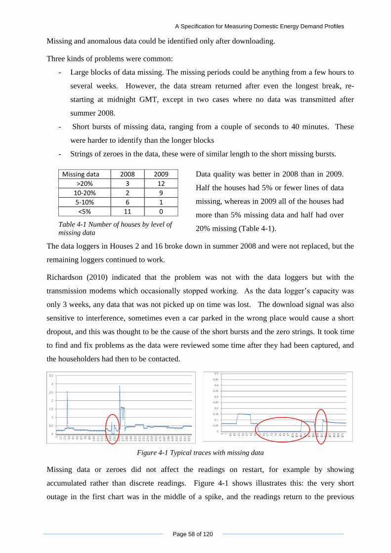
A Specification for Measuring Domestic Energy Demand Profiles
Page 58 of 120
Missing and anomalous data could be identified only after downloading.
Three kinds of problems were common:
- Large blocks of data missing. The missing periods could be anything from a few hours to
several weeks. However, the data stream returned after even the longest break, re-
starting at midnight GMT, except in two cases where no data was transmitted after
summer 2008.
- Short bursts of missing data, ranging from a couple of seconds to 40 minutes. These
were harder to identify than the longer blocks
- Strings of zeroes in the data, these were of similar length to the short missing bursts.
Missing data 2008 2009
>20% 3 12
10-20% 2 9
5-10% 6 1
<5% 11 0
Table 4-1 Number of houses by level of
missing data
Data quality was better in 2008 than in 2009.
Half the houses had 5% or fewer lines of data
missing, whereas in 2009 all of the houses had
more than 5% missing data and half had over
20% missing (Table 4-1).
The data loggers in Houses 2 and 16 broke down in summer 2008 and were not replaced, but the
remaining loggers continued to work.
Richardson (2010) indicated that the problem was not with the data loggers but with the
transmission modems which occasionally stopped working. As the data logger‟s capacity was
only 3 weeks, any data that was not picked up on time was lost. The download signal was also
sensitive to interference, sometimes even a car parked in the wrong place would cause a short
dropout, and this was thought to be the cause of the short bursts and the zero strings. It took time
to find and fix problems as the data were reviewed some time after they had been captured, and
the householders had then to be contacted.
Figure 4-1 Typical traces with missing data
Missing data or zeroes did not affect the readings on restart, for example by showing
accumulated rather than discrete readings. Figure 4-1 shows illustrates this: the very short
outage in the first chart was in the middle of a spike, and the readings return to the previous
A Specification for Measuring Domestic Energy Demand Profiles
Page 59 of 120
level. In the second chart, with a longer outage there may be a tiny blip on restart; however, it is
not big enough to affect the pattern. Missing data were therefore not corrected or interpolated,
they were just left out of averages.
One significant piece of context data was missing in the original files was that although the date
and time had been recorded, the day of the week was not – although this was not difficult to
reconstruct, it was time-consuming.
4.3 Data processing approach
The time series data for each house was first sorted by season and by day of week. Definition of
the seasons was according to (Elexon, 2011), but with winter split into two:
Winter 1: from 1 January, up to and including the day before the clock change from GMT to BST in March
Spring: the period from the day of clock change from GMT to BST in March, up to and including the Friday before the start of the summer period
Summer: the ten-week period before High Summer, starting on the sixteenth Saturday before the August Bank Holiday
High Summer: the period of six weeks and two days from the sixth Saturday before August Bank Holiday up to and including the Sunday following August Bank Holiday
Autumn: from the Monday after the August Bank Holiday, up to and including the day before the clock change from BST to GMT in October
Winter 2: from the day of clock change from British Summer Time (BST) to Greenwich Mean Time (GMT) in October, up to and including December 31st
This definition means that seasons are of unequal length, and the number of weeks can vary from
year to year except for Summer and High Summer. It was chosen because it does reflect
experience of how activity patterns actually vary over the year, with High Summer
corresponding to the school holiday period, and the start of winter and spring with abrupt
changes in daylight hours. The time-series analysis was done by season and by day of week;
Bank Holidays were treated as Sundays, in line with Elexon practice.
Each year‟s data contained an extra hour on a Sunday at the start for winter when the clocks
changed, and was missing an hour of data in the first Sunday in Spring when they were brought
forwards. Local time was used in all the analyses as this is what is important for people day to
day. In these analyses the extra hour‟s data was dropped (ie, the second set of data for 2-3am),
and the missing hour was treated as missing (ie, no data between 2-3am on the relevant day) As
the time change occurs when activity is lowest, this was not considered to introduce much error.
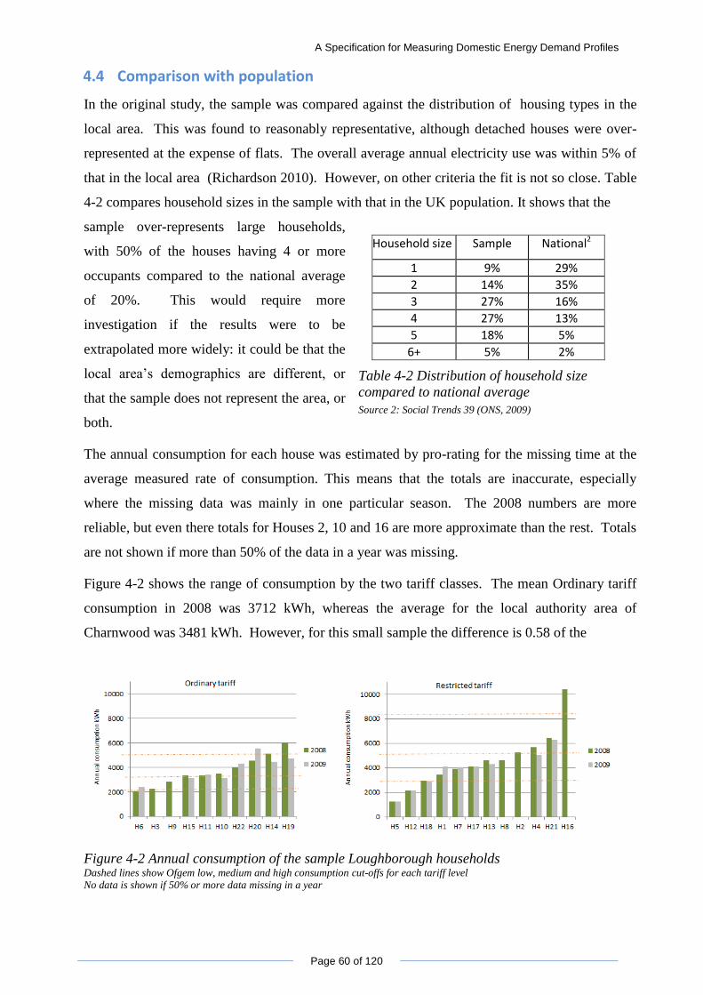
A Specification for Measuring Domestic Energy Demand Profiles
Page 60 of 120
4.4 Comparison with population
In the original study, the sample was compared against the distribution of housing types in the
local area. This was found to reasonably representative, although detached houses were over-
represented at the expense of flats. The overall average annual electricity use was within 5% of
that in the local area (Richardson 2010). However, on other criteria the fit is not so close. Table
4-2 compares household sizes in the sample with that in the UK population. It shows that the
sample over-represents large households,
with 50% of the houses having 4 or more
occupants compared to the national average
of 20%. This would require more
investigation if the results were to be
extrapolated more widely: it could be that the
local area‟s demographics are different, or
that the sample does not represent the area, or
both.
Household size Sample National2
1 9% 29%
2 14% 35%
3 27% 16%
4 27% 13%
5 18% 5%
6+ 5% 2%
Table 4-2 Distribution of household size
compared to national average
Source 2: Social Trends 39 (ONS, 2009)
The annual consumption for each house was estimated by pro-rating for the missing time at the
average measured rate of consumption. This means that the totals are inaccurate, especially
where the missing data was mainly in one particular season. The 2008 numbers are more
reliable, but even there totals for Houses 2, 10 and 16 are more approximate than the rest. Totals
are not shown if more than 50% of the data in a year was missing.
Figure 4-2 shows the range of consumption by the two tariff classes. The mean Ordinary tariff
consumption in 2008 was 3712 kWh, whereas the average for the local authority area of
Charnwood was 3481 kWh. However, for this small sample the difference is 0.58 of the
Figure 4-2 Annual consumption of the sample Loughborough households Dashed lines show Ofgem low, medium and high consumption cut-offs for each tariff level
No data is shown if 50% or more data missing in a year
A Specification for Measuring Domestic Energy Demand Profiles
Page 61 of 120
standard error. For the Restricted tariff households, the average is 4588 kWh/year, compared to
a Charnwood mean of 4671, and the difference is just 0.12 of the standard error. Restricted tariff
users make up 55% of the total sample, close to the Charnwood district council average of 50%.
In average electricity consumption terms therefore the sample represents of the bulk of the
population well.
Ordinary Restricted
Highest 10% 8%
High 50% 25%
Low 30% 50%
Lowest 10% 17%
Table 4-3 Distribution of sample houses by
Ofgem consumption band
Figure 4-2 shows the range of consumption
by tariff type, with the Ofgem band cut-offs
shown as dotted lines. It would appear that
the sample under-represents the very highest
consumers – another potential limitation to
how far the data can be generalised. None of
the ordinary tariff houses would fall into Elexon‟s highest band, over 7,500 kWh per year.
Another perspective on the range of consumption
is given on the Lorenz curve in Figure 4-3. This
compares actual cumulative use by houses,
ordered from least to highest, against the straight
line that would represent equal consumption. The
more the actual line bows away from the straight,
the greater the range of use between highest and
least. The Gini coefficient of this distribution is
0.24, which indicates the level of inequality closer
to that of Norway (G=0.19) than the US (G=0.37).
Figure 4-3 Cumulative consumption across
sample houses (Lorenz curve)
Ownership Sample National
Non-electric central heating 91% 85%
Electric oven 68% 62%
Electric hob 14% 46%
Dishwasher 68% 38%
Tumble dryer 36% 59%
No. of cold app/house 1.8 1.5
No. TVs/house 1.7 2.2
Households with computers 100% 72%
Table 4-4 Appliance ownership in sample compared
to national statistics for 2008 Source: (DECC, 2010)
The level of appliance ownership in the
sample is compared to national
ownership statistics in Table 1-1Table 4-4.
If end-use had been measured, it would
be a reasonable expectation that a lower
proportion of electricity was used for
space heating and cooking, but a higher
proportion for cold appliances and
computing.
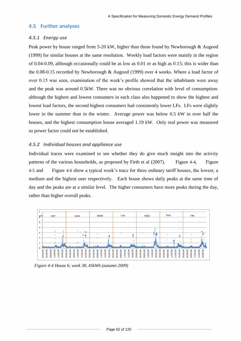
A Specification for Measuring Domestic Energy Demand Profiles
Page 62 of 120
4.5 Further analyses
4.5.1 Energy use
Peak power by house ranged from 5-20 kW, higher than those found by Newborough & Augood
(1999) for similar houses at the same resolution. Weekly load factors were mainly in the region
of 0.04-0.09, although occasionally could be as low as 0.01 or as high as 0.15; this is wider than
the 0.08-0.15 recorded by Newborough & Augood (1999) over 4 weeks. Where a load factor of
over 0.15 was seen, examination of the week‟s profile showed that the inhabitants were away
and the peak was around 0.5kW. There was no obvious correlation with level of consumption:
although the highest and lowest consumers in each class also happened to show the highest and
lowest load factors, the second highest consumers had consistently lower LFs. LFs were slightly
lower in the summer than in the winter. Average power was below 0.5 kW in over half the
houses, and the highest consumption house averaged 1.19 kW. Only real power was measured
so power factor could not be established.
4.5.2 Individual houses and appliance use
Individual traces were examined to see whether they do give much insight into the activity
patterns of the various households, as proposed by Firth et al (2007). Figure 4-4, Figure
4-5 and Figure 4-6 show a typical week‟s trace for three ordinary tariff houses, the lowest, a
medium and the highest user respectively. Each house shows daily peaks at the same time of
day and the peaks are at a similar level. The higher consumers have more peaks during the day,
rather than higher overall peaks.
Figure 4-4 House 6, week 38, 45kWh (autumn 2009)
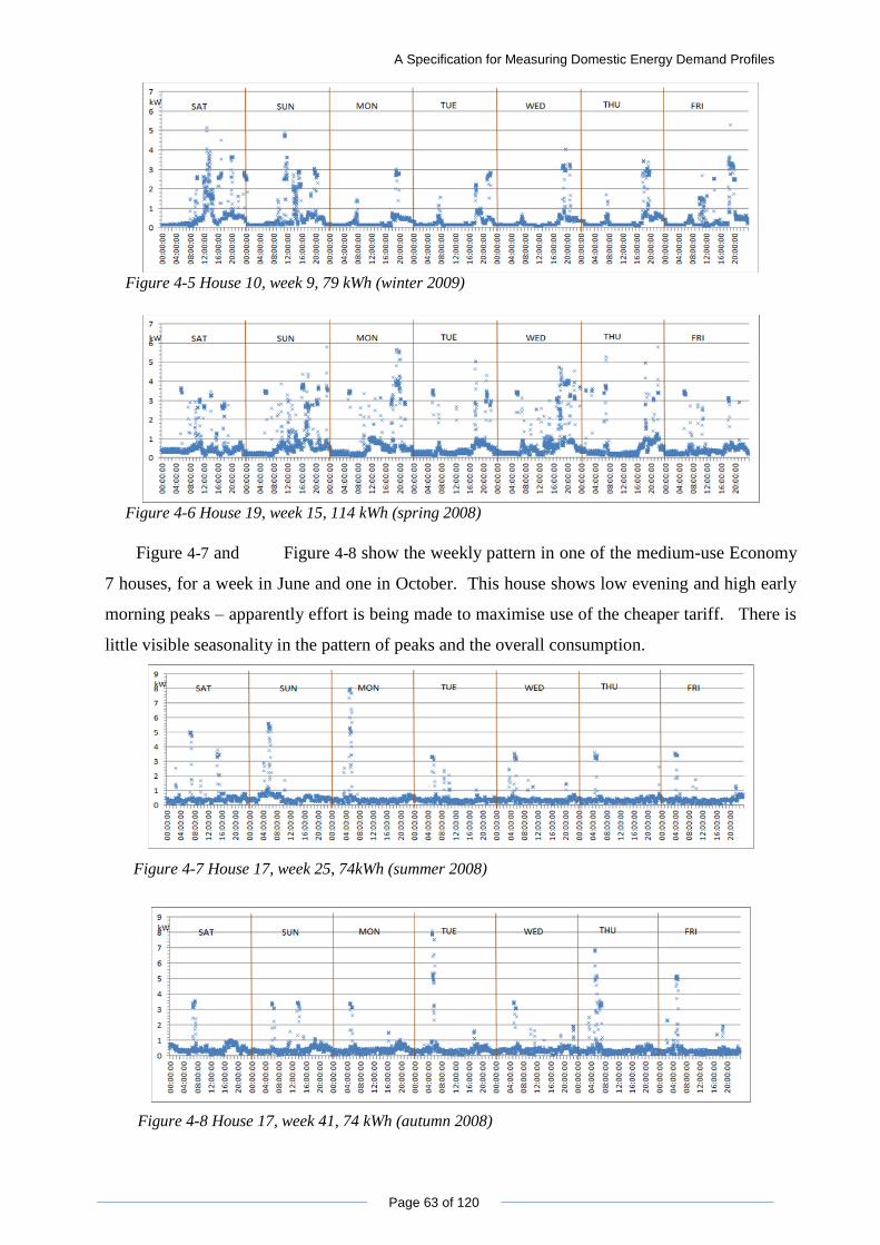
A Specification for Measuring Domestic Energy Demand Profiles
Page 63 of 120
Figure 4-5 House 10, week 9, 79 kWh (winter 2009)
Figure 4-6 House 19, week 15, 114 kWh (spring 2008)
Figure 4-7 and Figure 4-8 show the weekly pattern in one of the medium-use Economy
7 houses, for a week in June and one in October. This house shows low evening and high early
morning peaks – apparently effort is being made to maximise use of the cheaper tariff. There is
little visible seasonality in the pattern of peaks and the overall consumption.
Figure 4-7 House 17, week 25, 74kWh (summer 2008)
Figure 4-8 House 17, week 41, 74 kWh (autumn 2008)
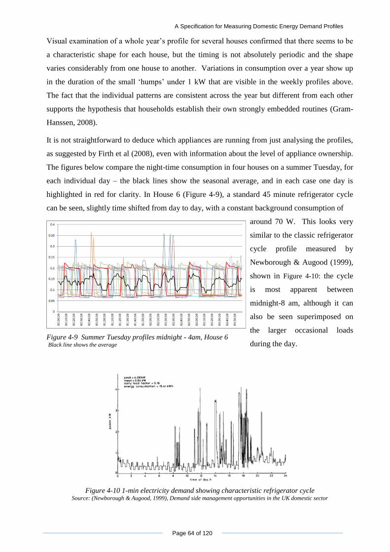
A Specification for Measuring Domestic Energy Demand Profiles
Page 64 of 120
Visual examination of a whole year‟s profile for several houses confirmed that there seems to be
a characteristic shape for each house, but the timing is not absolutely periodic and the shape
varies considerably from one house to another. Variations in consumption over a year show up
in the duration of the small „humps‟ under 1 kW that are visible in the weekly profiles above.
The fact that the individual patterns are consistent across the year but different from each other
supports the hypothesis that households establish their own strongly embedded routines (Gram-
Hanssen, 2008).
It is not straightforward to deduce which appliances are running from just analysing the profiles,
as suggested by Firth et al (2008), even with information about the level of appliance ownership.
The figures below compare the night-time consumption in four houses on a summer Tuesday, for
each individual day – the black lines show the seasonal average, and in each case one day is
highlighted in red for clarity. In House 6 (Figure 4-9), a standard 45 minute refrigerator cycle
can be seen, slightly time shifted from day to day, with a constant background consumption of
Figure 4-9 Summer Tuesday profiles midnight - 4am, House 6 Black line shows the average
around 70 W. This looks very
similar to the classic refrigerator
cycle profile measured by
Newborough & Augood (1999),
shown in Figure 4-10: the cycle
is most apparent between
midnight-8 am, although it can
also be seen superimposed on
the larger occasional loads
during the day.
Figure 4-10 1-min electricity demand showing characteristic refrigerator cycle Source: (Newborough & Augood, 1999), Demand side management opportunities in the UK domestic sector
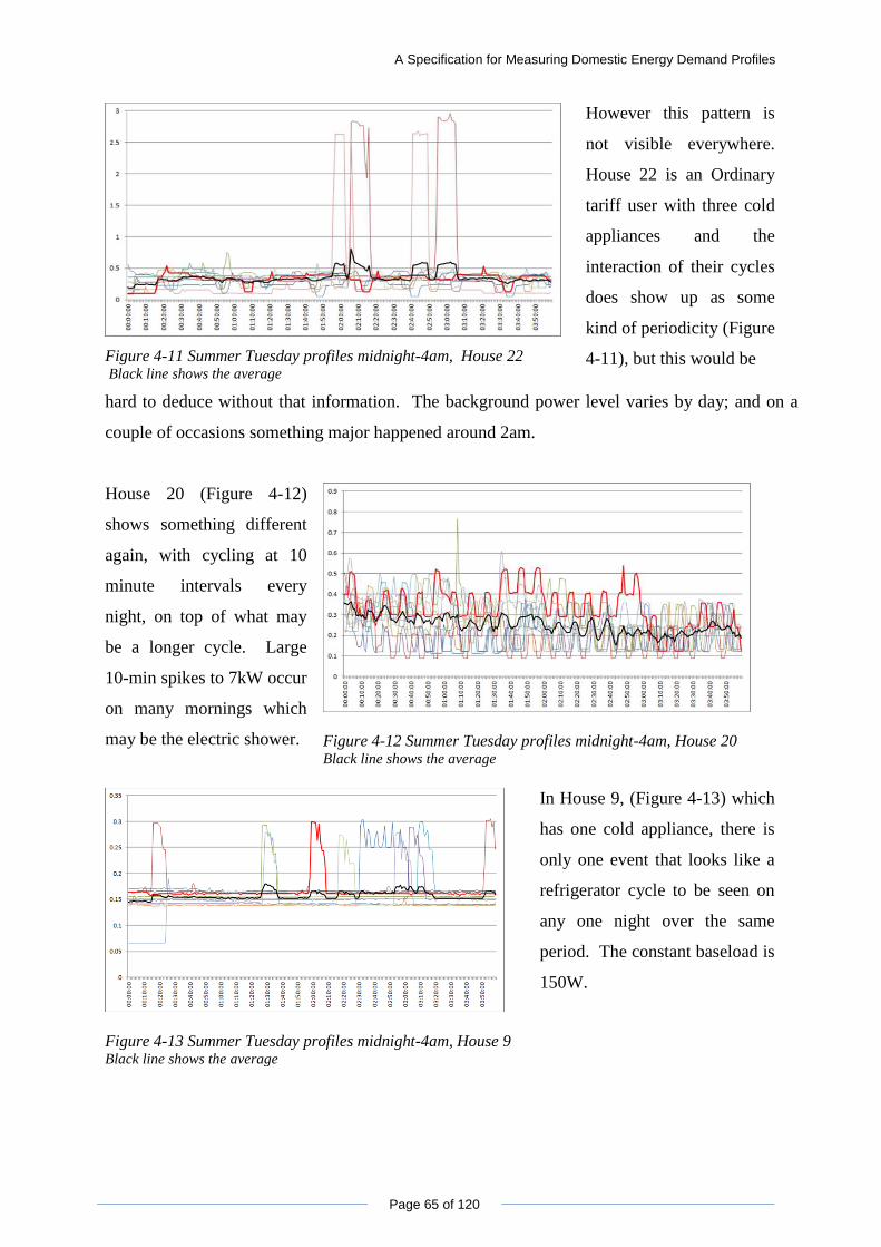
A Specification for Measuring Domestic Energy Demand Profiles
Page 65 of 120
Figure 4-11 Summer Tuesday profiles midnight-4am, House 22 Black line shows the average
However this pattern is
not visible everywhere.
House 22 is an Ordinary
tariff user with three cold
appliances and the
interaction of their cycles
does show up as some
kind of periodicity (Figure
4-11), but this would be
hard to deduce without that information. The background power level varies by day; and on a
couple of occasions something major happened around 2am.
House 20 (Figure 4-12)
shows something different
again, with cycling at 10
minute intervals every
night, on top of what may
be a longer cycle. Large
10-min spikes to 7kW occur
on many mornings which
may be the electric shower.
Figure 4-12 Summer Tuesday profiles midnight-4am, House 20 Black line shows the average
Figure 4-13 Summer Tuesday profiles midnight-4am, House 9 Black line shows the average
In House 9, (Figure 4-13) which
has one cold appliance, there is
only one event that looks like a
refrigerator cycle to be seen on
any one night over the same
period. The constant baseload is
150W.
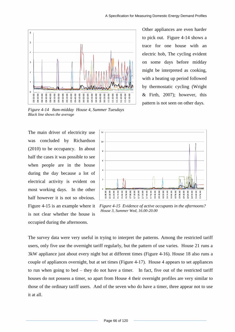
A Specification for Measuring Domestic Energy Demand Profiles
Page 66 of 120
Figure 4-14 8am-midday House 4, Summer Tuesdays Black line shows the average
Other appliances are even harder
to pick out. Figure 4-14 shows a
trace for one house with an
electric hob, The cycling evident
on some days before midday
might be interpreted as cooking,
with a heating up period followed
by thermostatic cycling (Wright
& Firth, 2007); however, this
pattern is not seen on other days.
The main driver of electricity use
was concluded by Richardson
(2010) to be occupancy. In about
half the cases it was possible to see
when people are in the house
during the day because a lot of
electrical activity is evident on
most working days. In the other
half however it is not so obvious.
Figure 4-15 is an example where it
is not clear whether the house is
occupied during the afternoons.
Figure 4-15 Evidence of active occupants in the afternoons? House 3, Summer Wed, 16.00-20.00
The survey data were very useful in trying to interpret the patterns. Among the restricted tariff
users, only five use the overnight tariff regularly, but the pattern of use varies. House 21 runs a
3kW appliance just about every night but at different times (Figure 4-16). House 18 also runs a
couple of appliances overnight, but at set times (Figure 4-17). House 4 appears to set appliances
to run when going to bed – they do not have a timer. In fact, five out of the restricted tariff
houses do not possess a timer, so apart from House 4 their overnight profiles are very similar to
those of the ordinary tariff users. And of the seven who do have a timer, three appear not to use
it at all.
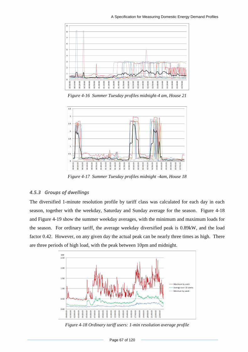
A Specification for Measuring Domestic Energy Demand Profiles
Page 67 of 120
Figure 4-16 Summer Tuesday profiles midnight-4 am, House 21
Figure 4-17 Summer Tuesday profiles midnight -4am, House 18
4.5.3 Groups of dwellings
The diversified 1-minute resolution profile by tariff class was calculated for each day in each
season, together with the weekday, Saturday and Sunday average for the season. Figure 4-18
and Figure 4-19 show the summer weekday averages, with the minimum and maximum loads for
the season. For ordinary tariff, the average weekday diversified peak is 0.89kW, and the load
factor 0.42. However, on any given day the actual peak can be nearly three times as high. There
are three periods of high load, with the peak between 10pm and midnight.
Figure 4-18 Ordinary tariff users: 1-min resolution average profile
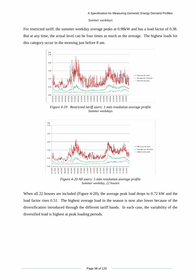
A Specification for Measuring Domestic Energy Demand Profiles
Page 68 of 120
Summer weekdays
For restricted tariff, the summer weekday average peaks at 0.98kW and has a load factor of 0.38.
But at any time, the actual level can be four times as much as the average. The highest loads for
this category occur in the morning just before 8 am.
Figure 4-19 Restricted tariff users: 1-min resolution average profile Summer weekdays
Figure 4-20 All users: 1-min resolution average profile Summer weekday, 22 houses
When all 22 houses are included (Figure 4-20), the average peak load drops to 0.72 kW and the
load factor rises 0.51. The highest average load in the season is now also lower because of the
diversification introduced through the different tariff bands. In each case, the variability of the
diversified load is highest at peak loading periods.
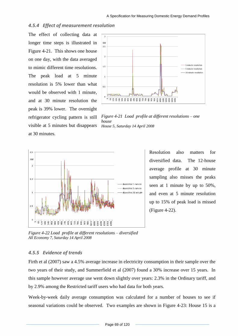
A Specification for Measuring Domestic Energy Demand Profiles
Page 69 of 120
4.5.4 Effect of measurement resolution
The effect of collecting data at
longer time steps is illustrated in
Figure 4-21. This shows one house
on one day, with the data averaged
to mimic different time resolutions.
The peak load at 5 minute
resolution is 5% lower than what
would be observed with 1 minute,
and at 30 minute resolution the
peak is 39% lower. The overnight
refrigerator cycling pattern is still
visible at 5 minutes but disappears
at 30 minutes.
Figure 4-21 Load profile at different resolutions – one
house House 5, Saturday 14 April 2008
Figure 4-22 Load profile at different resolutions – diversified All Economy 7, Saturday 14 April 2008
Resolution also matters for
diversified data. The 12-house
average profile at 30 minute
sampling also misses the peaks
seen at 1 minute by up to 50%,
and even at 5 minute resolution
up to 15% of peak load is missed
(Figure 4-22).
4.5.5 Evidence of trends
Firth et al (2007) saw a 4.5% average increase in electricity consumption in their sample over the
two years of their study, and Summerfield et al (2007) found a 30% increase over 15 years. In
this sample however average use went down slightly over years: 2.3% in the Ordinary tariff, and
by 2.9% among the Restricted tariff users who had data for both years.
Week-by-week daily average consumption was calculated for a number of houses to see if
seasonal variations could be observed. Two examples are shown in Figure 4-23: House 15 is a
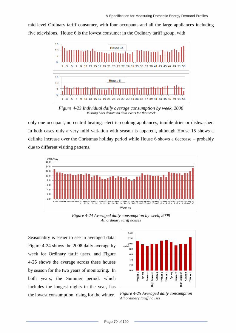
A Specification for Measuring Domestic Energy Demand Profiles
Page 70 of 120
mid-level Ordinary tariff consumer, with four occupants and all the large appliances including
five televisions. House 6 is the lowest consumer in the Ordinary tariff group, with
Figure 4-23 Individual daily average consumption by week, 2008 Missing bars denote no data exists for that week
only one occupant, no central heating, electric cooking appliances, tumble drier or dishwasher.
In both cases only a very mild variation with season is apparent, although House 15 shows a
definite increase over the Christmas holiday period while House 6 shows a decrease – probably
due to different visiting patterns.
Figure 4-24 Averaged daily consumption by week, 2008 All ordinary tariff houses
Seasonality is easier to see in averaged data:
Figure 4-24 shows the 2008 daily average by
week for Ordinary tariff users, and Figure
4-25 shows the average across these houses
by season for the two years of monitoring. In
both years, the Summer period, which
includes the longest nights in the year, has
the lowest consumption, rising for the winter.
Figure 4-25 Averaged daily consumption All ordinary tariff houses
0.0
2.0
4.0
6.0
8.0
10.0
12.0
14.0
16.0
0 1 2 3 4 5 6 7 8 91
01
11
21
31
41
51
61
71
81
92
02
12
22
32
42
52
62
72
82
93
03
13
23
33
43
53
63
73
83
94
04
14
24
34
44
54
64
74
84
95
05
15
2
kWh/day
Week no
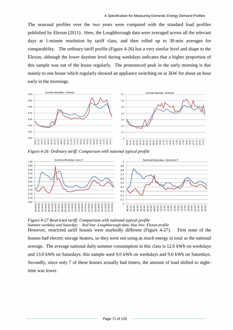
A Specification for Measuring Domestic Energy Demand Profiles
Page 71 of 120
The seasonal profiles over the two years were compared with the standard load profiles
published by Elexon (2011). Here, the Loughborough data were averaged across all the relevant
days at 1-minute resolution by tariff class, and then rolled up to 30-min averages for
comparability. The ordinary tariff profile (Figure 4-26) has a very similar level and shape to the
Elexon, although the lower daytime level during weekdays indicates that a higher proportion of
this sample was out of the house regularly. The pronounced peak in the early morning is due
mainly to one house which regularly showed an appliance switching on at 3kW for about an hour
early in the mornings.
Figure 4-26 Ordinary tariff: Comparison with national typical profile
Figure 4-27 Restricted tariff: Comparison with national typical profile Summer weekday and Saturday; Red line: Loughborough data, blue line: Elexon profile
However, restricted tariff houses were markedly different (Figure 4-27). First none of the
houses had electric storage heaters, so they were not using as much energy in total as the national
average. The average national daily summer consumption in this class is 12.6 kWh on weekdays
and 13.0 kWh on Saturdays: this sample used 9.0 kWh on weekdays and 9.6 kWh on Saturdays.
Secondly, since only 7 of these houses actually had timers, the amount of load shifted to night-
time was lower.
A Specification for Measuring Domestic Energy Demand Profiles
Page 72 of 120
Figure 4-28 Electricity consumption per
person by household size
The study of low-energy houses by Gill et
al (2011) noted a decreasing tend in energy
use per person, with increasing household
size. This is not readily apparent from the
Loughborough sample, where without the
single outlier point near 3000 kWh/person,
no trend at all would be visible (Figure
4-28). Both lowest and highest
consumption per person are in restricted
tariff households – the former is the more
surprising finding.
The average daily consumption was
plotted against appliance ownership,
trying out a number of different
ways of counting appliances. Figure
4-29 shows the best correlation,
which is with large appliances
owned. These comprised electric
shower, refrigerators and freezers,
hobs and ovens, washing machines,
tumble driers and dishwashers, and
TVs and computers.
Figure 4-29 Electricity consumption and large
appliance ownership
Some kind of trend is evident here, although it is not enormously strong, and the correlation is
only 54%. Table 4-5 shows the ownership of various large appliances within the top and bottom
quartiles in the whole sample. Although there is one case where electric heating is used, this g
No. among
highest 5
consumers
No. among
lowest 5
consumers
No. in all
houses
Electric heating 1 0 2
Electric showers 2 3 9
Electric hobs 1 0 3
Electric ovens 5 1 15
Tumble driers 0 3 8
Dishwashers 1 4 15
Av. Occupancy 1.8 3.8 3.45
Table 4-5 Ownership of large appliances in top and bottom
quartile
house is in fact only the 5th
highest
user. Ownership of electric showers
is fairly evenly spread in the
rankings. The only appliance where
ownership and energy use ranking
seem to be correlated is electric
ovens, where 9 of the top 11
consumers have them, and
A Specification for Measuring Domestic Energy Demand Profiles
Page 73 of 120
dishwashers, which are owned by 10 of the top 11. It is however significant that the bottom
quartile has low numbers of occupants while the top quartile has higher.
4.6 Conclusions from data analysis
This was a relatively homogeneous sample group, reflecting the average users in the district but
not the extremely low or extremely high consumers. The lack of the latter limits the extent to
which the outcomes can be extrapolated to the wider area. One large, regular user in the sample
did affect the overall shape, even over a 22-house group.
They give a reasonably typical picture of the pattern of ordinary tariff users but less so for
restricted tariff users. In the sample, many of the people who have the Economy 7 tariff do not
actually make use of it, especially not for heating.
It is harder to tell which appliances are being used appliances from time series readings than
implied in the literature, even with survey data is available on which household owns how many
of each. One-minute resolution data gives a different picture of the size of peak loads even when
diversified over a group of houses. Even a five-minute average loses around 15% of the peak.
Total electricity use did increase as the household size went up. However, there was no
observable trend in the amount used per person with increasing household size. There is some
correlation between large appliances owned and total electricity use, but this is weak.
Ownership of dishwashers and electric ovens in particular was significantly higher among the
highest users than the lowest. There was no evidence of increasing usage from one year to the
next.
The fact that only electricity was measured means that energy consumption is not truly
comparable across the various houses. The proportion of electrical energy used for hot water
and for cooking, in particular, will be very different in a house that has electric showers, and
electric oven and hob than one where it is not. However, since only total electricity use was
measured, and end-uses and other fuel consumption were not, it is not possible to use this data
for modelling what-if scenarios on fuel switching or demand management.
The aim of the original programme was to validate a model of electricity demand for a group of
houses, in order to carry out network analysis, and it met this aim well. The present analysis
exercise has demonstrated is that it is possible to use that same data for other investigations and
purposes. The survey information was very important in enabling this.

A Specification for Measuring Domestic Energy Demand Profiles
Page 74 of 120
5 Specification for a standard, comprehensive data set
Data collection programmes always have a specific purpose, with limited budgets and people
available, so they measure only that which is strictly required. However, any such exercise is
time-consuming both to set up and carry out, so there ought to be some value in thinking beyond
the specific demands of the question in hand. This section outlines the requirements for a
standard, comprehensive data set, based on the findings in Chapters 3 and 4, and proposes a
specification for data collection whose outcome could be used more widely.
5.1 Measurement plan requirements
The requirements for the measurement plan are:
- Measure inputs for all fuels – even where this can only be approximated.
- Measure consumption by end-use – by groups of appliances that are used together where
possible, individual appliances where not.
- Prioritise based on the importance of each in terms of: potential for time-shifting; potential
for change of fuel; overall consumption; contribution to peak load
- Measure inputs/activity drivers as well as outputs / consumption
- Be consistent in what is measured, frequency and accuracy level
- Understand the individual context of each household through a structured survey at the
start, preferably face-to-face
- Tailor the plan to the context so that all the important end-uses are covered without
collecting too much low-impact data
- Collect and analyse the data quickly, preferably in real time, so that anomalies and
problems can be investigated
- Use consistent categories for context and analysis
- Make the cleansed data available publicly as well as the analyses, but without personal
data that could identify the participants
- Aim for a quantity of data that could reasonably be expected to be collected by monitoring
programmes without a large incremental cost
A Specification for Measuring Domestic Energy Demand Profiles
Page 75 of 120
5.2 Data
The data items are shown in two categories: those which are most important to collect
consistently in every case, and those which would be very useful but could be dropped if
circumstances dictate. Also, survey information includes some which can be gathered
effectively only through face to face interviews and not by a questionnaire. In the sections
below, the second-tier measurements, and the interview-only questions, are shown in italics.
If resources are constrained, experience from other programmes suggests that adequate results
can be obtained from a data collection plan which covers some of the sample properties in detail,
and the rest at a reduced level. This would however restrict the usefulness of the data for
statistics and some model calibration.
5.2.1 Fuel use and general context
This is data on the house and its occupants that gives the context for energy use, and its overall
consumption of different fuels that ties together the end-use level measurements. The general
survey includes a full set of context data. The survey on attitudes to energy use lists the areas to
be covered in an interview; the actual questions will need to be couched more colloquially and
follow-up and clarification questions designed.
MEASUREMENT – FUEL USE
Gas: utility revenue meter readings
Electricity: utility revenue meter readings
Oil: tank level measured via hydrostatic gauge, together with delivery records of volume and specific gravity
Bulk LPG: tank level gauge or electronic monitor – most domestic tanks are equipped for telemetry by the supplier
Solid fuel: log of volumes used, with delivery records of volume
On-site generation: output of generator for electricity, and/or temperature and flow rate for hot water
SURVEY – GENERAL DATA
Location to level of 1st three digits of post code
Number of people in the household, and their ages and stage of life
Occupancy pattern: morning/ lunchtime/ afternoon/ early evening/ late evening; hours of employment and schooling
Highest education level in household: no qualifications/GCSE or A level/ vocational qualification/ University degree
Household disposable income level, by week: grouped by 10th, 50th and 90th percentile in Social Trends (currently: under £200/200-400/400-700/over 700)
A Specification for Measuring Domestic Energy Demand Profiles
Page 76 of 120
Property type - house, bungalow, flat; detached, terraced, semi; top, middle, ground floor
Approximate floor area (this can also be estimated from Ordnance Survey Master map data)
Number of living and bedrooms – including any bedrooms used as living rooms
Main heating system, type and fuel
Gas, electricity and any other fuel usage from bills for the last 12 months; time-of-use tariff if any
SURVEY – ATTITUDES TO ENERGY USE
How much time and attention is given to managing energy use and cost;
What energy efficiency measures have been put in place; how much did they cost to implement; what else would be good to do; what are barriers to this
Why was the particular electricity/gas provider and tariff chosen – what other providers and tariffs considered; how often looked at
How important are energy costs in overall monthly or weekly budget
What information would be useful / interesting concerning cost and impact of energy use;
How much interest in environmental issues; what changes this has made to lifestyle; willingness to make other changes; where the line is drawn
5.2.2 Space Heating
Space heating input will not equal to fuel input, partly because of combustion inefficiency and
the fact that some heat may escape to the outside (for example through under-floor pipes); and
partly because the heating fuel generally also supplies hot water and cooking needs.
For output measures, the minimum are temperature in living rooms and one bedroom However,
if more than one room is regularly used as a living room – for example, teenagers entertaining
and watching TV in their bedroom - then the temperature there should also be measured. If the
thermostat is in the hall, the temperature near it should also be read as this is an area where
householders do not necessarily know the facts.
MEASUREMENT
central heating: heating circuit temperature and flow rate
fixed or portable electric or storage heaters: appliance load(s)
fixed gas heaters: gas flow rate(s)
portable LPG heaters: status of each heating panel from panel temperature:
solid fuel: log books of quantity used; moisture content measurements; stove temperature measurements
external conditions- temperature, RH, wind speed and direction, direct and diffuse solar radiation – however these can be measured in common or taken from nearby met office
A Specification for Measuring Domestic Energy Demand Profiles
Page 77 of 120
measurements
living room temperature and relative humidity
main bedroom temperature
temperature in additional ‘living area’
temperature beside thermostat
The first set of survey questions are attributes of the house itself: its size and orientation,
exposure level, and details about its construction that together determine its thermal mass, heat
transfer behaviour and level of airtightness. The second set concerns how the heating – and
where it exists, cooling - system is used. The third set is about family habits and perceptions of
what is comfortable.
SURVEY
general surroundings and orientation of house
floor area, ceiling height, window size
external wall, floor, and roof materials
insulation level, including any improvements made since building
on-site generation if any
type of boiler, age and rating
whether air conditioning is used, and under what circumstances
control system and thermostat settings, thermostat location – awareness, how often changed, is it perceived to be working properly
secondary heating fuel, if any, and pattern of use
seasonal routines and changes – regular visitors or B&B in the summer or regularly away for part or winter etc.
pattern of room use – does the family sit in one place evenings and weekends, or are they dispersed
comfort perceptions of different parts of the house: temperature, stuffiness, draughtiness, problem areas such as damp or mould
5.2.3 Hot Water
Hot water can be supplied either from the heating system or by a dedicated boiler; it can be
stored in a tank or used directly. Although there are not quite so many permutations as with
space heating, the measurement plan needs to be flexible to accommodate individual differences.
Drivers of hot water used are the number of residents, temperature of the incoming water, type of
appliances used such as power showers, or washing machines or dishwashers with a hot water
intake. Personal preferences are important in terms of timing
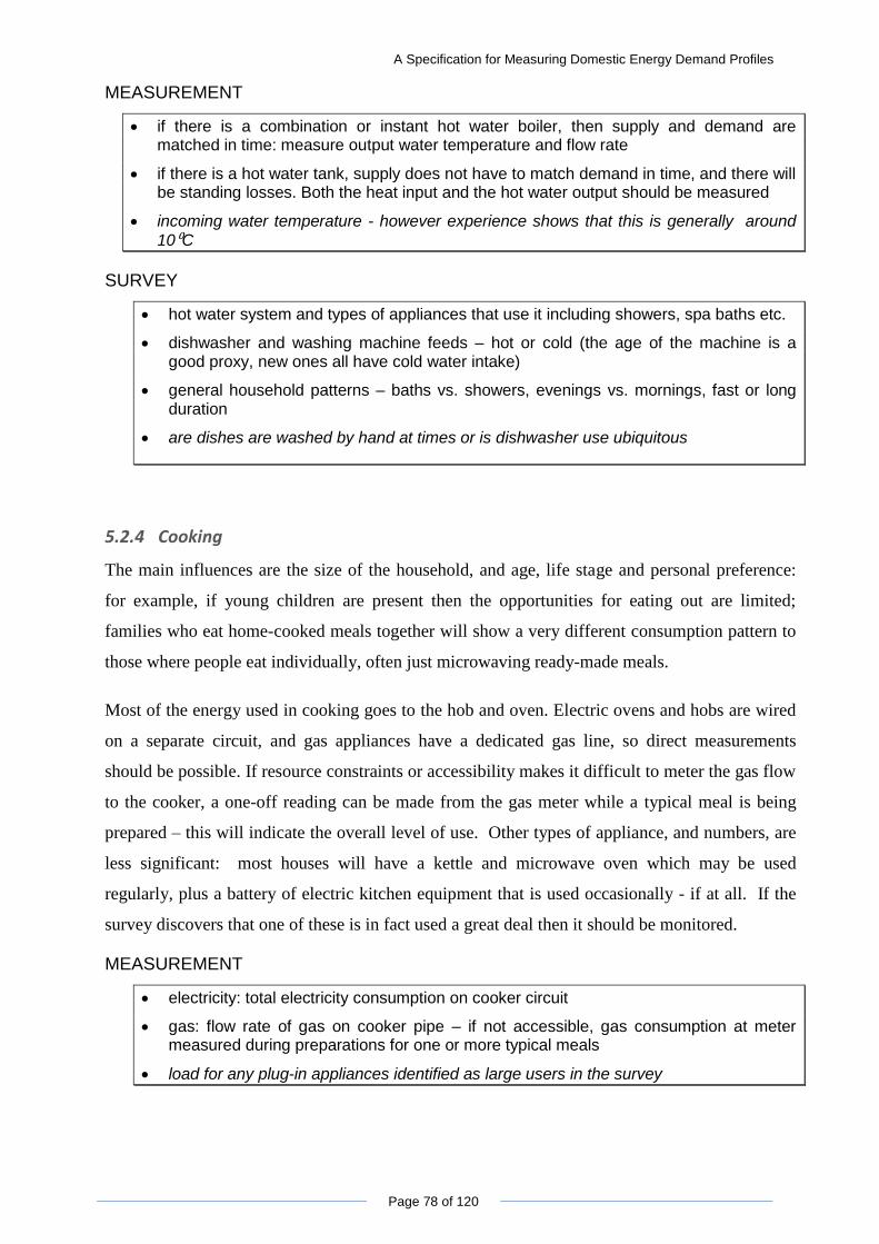
A Specification for Measuring Domestic Energy Demand Profiles
Page 78 of 120
MEASUREMENT
if there is a combination or instant hot water boiler, then supply and demand are matched in time: measure output water temperature and flow rate
if there is a hot water tank, supply does not have to match demand in time, and there will be standing losses. Both the heat input and the hot water output should be measured
incoming water temperature - however experience shows that this is generally around
10⁰C
SURVEY
hot water system and types of appliances that use it including showers, spa baths etc.
dishwasher and washing machine feeds – hot or cold (the age of the machine is a good proxy, new ones all have cold water intake)
general household patterns – baths vs. showers, evenings vs. mornings, fast or long duration
are dishes are washed by hand at times or is dishwasher use ubiquitous
5.2.4 Cooking
The main influences are the size of the household, and age, life stage and personal preference:
for example, if young children are present then the opportunities for eating out are limited;
families who eat home-cooked meals together will show a very different consumption pattern to
those where people eat individually, often just microwaving ready-made meals.
Most of the energy used in cooking goes to the hob and oven. Electric ovens and hobs are wired
on a separate circuit, and gas appliances have a dedicated gas line, so direct measurements
should be possible. If resource constraints or accessibility makes it difficult to meter the gas flow
to the cooker, a one-off reading can be made from the gas meter while a typical meal is being
prepared – this will indicate the overall level of use. Other types of appliance, and numbers, are
less significant: most houses will have a kettle and microwave oven which may be used
regularly, plus a battery of electric kitchen equipment that is used occasionally - if at all. If the
survey discovers that one of these is in fact used a great deal then it should be monitored.
MEASUREMENT
electricity: total electricity consumption on cooker circuit
gas: flow rate of gas on cooker pipe – if not accessible, gas consumption at meter measured during preparations for one or more typical meals
load for any plug-in appliances identified as large users in the survey
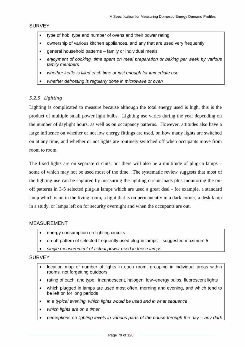
A Specification for Measuring Domestic Energy Demand Profiles
Page 79 of 120
SURVEY
type of hob, type and number of ovens and their power rating
ownership of various kitchen appliances, and any that are used very frequently
general household patterns – family or individual meals
enjoyment of cooking, time spent on meal preparation or baking per week by various family members
whether kettle is filled each time or just enough for immediate use
whether defrosting is regularly done in microwave or oven
5.2.5 Lighting
Lighting is complicated to measure because although the total energy used is high, this is the
product of multiple small power light bulbs. Lighting use varies during the year depending on
the number of daylight hours, as well as on occupancy patterns. However, attitudes also have a
large influence on whether or not low energy fittings are used, on how many lights are switched
on at any time, and whether or not lights are routinely switched off when occupants move from
room to room.
The fixed lights are on separate circuits, but there will also be a multitude of plug-in lamps –
some of which may not be used most of the time. The systematic review suggests that most of
the lighting use can be captured by measuring the lighting circuit loads plus monitoring the on-
off patterns in 3-5 selected plug-in lamps which are used a great deal - for example, a standard
lamp which is on in the living room, a light that is on permanently in a dark corner, a desk lamp
in a study, or lamps left on for security overnight and when the occupants are out.
MEASUREMENT
energy consumption on lighting circuits
on-off pattern of selected frequently used plug-in lamps – suggested maximum 5
single measurement of actual power used in these lamps
SURVEY
location map of number of lights in each room, grouping in individual areas within rooms, not forgetting outdoors
rating of each, and type: incandescent, halogen, low–energy bulbs, fluorescent lights
which plugged in lamps are used most often, morning and evening, and which tend to be left on for long periods
in a typical evening, which lights would be used and in what sequence
which lights are on a timer
perceptions on lighting levels in various parts of the house through the day – any dark
A Specification for Measuring Domestic Energy Demand Profiles
Page 80 of 120
areas where light is generally left on most of the day
replacement bulbs – are low energy versions routinely sought out, if not why
5.2.6 Cold Appliances
Households will have one or more cold appliances which are on all the time: refrigerators,
freezers, fridge freezers and drinks coolers. These consume electricity in a cyclical pattern over
40 minutes-1 hour, at a more or less constant rate unless they are unsuitable location or are being
left open regularly when in use. If resources are constrained, a reasonable approximation can be
made by monitoring the on-off periods together with a one-off measurement of the power drawn.
MEASUREMENT
appliance load for each OR
appliance on-off cycle especially if a refrigerator is in an unsuitable position, or if it is a large American style fridge with icemaker PLUS
check actual power consumption cycle manually for 1 hour during survey
SURVEY
number, age, energy consumption rating and efficiency rating of freezers, fridges, and chiller
location – whether next to cooker or in cool utility room
habits of use – temperature setting, how frequently opened during day, leaving door open or closed when filling shelves, whether defrosted regularly
5.2.7 Wet appliances
Dishwashers, washing machines and tumble driers are heavy electricity consumers – they draw
high peak power, and have long cycle times. Their energy use per cycle varies depending on the
cycle length and temperature setting, and also on whether they take in hot as well as cold water.
However their total contribution to household energy depends on household size, attitudes and
practices. For example, some households who have dishwashers may choose to use them all the
time whether they are full or not, others will prefer to wash small loads by hand and only deploy
the machine when there is a large party. If clothes drying takes place indoors regularly, the
heating system provides the latent energy input to evaporate water, and the humidity in the
drying area will also increase.
A Specification for Measuring Domestic Energy Demand Profiles
Page 81 of 120
MEASUREMENT
Consumption of each separate appliance: washing machine, dishwasher, tumble dryer
Temperature and relative humidity in drying area
SURVEY
number and energy consumption rating of appliances
hot or cold water intake of appliances
number of times a week each is used, and temperature setting and cycle used most often
preferences for dishwashing – by hand at times, or machine all the time, full or part loads
preferences for clothes drying – indoors, outdoors, by machine all the time; full or part loads
timing of when machines run – whether planned, for example to make use of overnight tariffs or to fit in with a schedule, or random, as and when enough dirty clothes are collected
willingness to allow time-shifting of when loads are run, and by how much; how big would the tariff discount need to be
5.2.8 Consumer electronics
Televisions and appliances associated with them such as speakers, set top boxes, games consoles
and DVD payers is the highest growth area of household energy. Many households have
multiple groups of these, in use simultaneously as different family members pursue their own
activities in different rooms. Energy use depends partly on how many appliances there are and
their power rating, but also very much on how they are used – whether they are the main form of
entertainment, as a constant background to other activities, whether they are switched off or on
standby when not in use. The survey should establish the number of measurements needed: the
ideal situation is where the whole group is plugged in together via a distributor board.
MEASUREMENT
Consumption of main group of related appliances: TV/set top box/DVD – which are often plugged in at the same place and used together
Consumption of secondary group(s) e.g. in kitchen or in teenagers’ bedroom
SURVEY
number of TVs, size and type: CRT/plasma/LCD/LED
location map of other related appliances e.g. speakers, set top box, DVD, games console
night-time pattern of use - standby or switched off overnight
daytime pattern of use of TV and associated appliances – one or several on at one time; left on, standby or switched off when not watched during the day,
average hours each TV is watched
A Specification for Measuring Domestic Energy Demand Profiles
Page 82 of 120
5.2.9 Computers and other miscellaneous appliances
The extent to which computers and other miscellaneous devices contribute to a household‟s
energy use is not possible to predict in advance. If someone in the house is regularly working
from home, then the computer and associated peripherals may be significant. If the house has a
sauna or hot tub, these will probably be big consumers – unless they are never used. Other
applications may not be so obvious - for example, the instance highlighted in Chapter 6 where
the security system turned out to be the single largest energy using appliance in the house. Other
things to notice are power-consuming hobbies – over the last 6 months the author has been in
houses which contained respectively: a sauna; a greenhouse heater; a pottery kiln; a hot tub; and
a professional bread oven, all of which were in regular use. The survey is essential in
establishing which if any appliances should be monitored
MEASUREMENT
Consumption of appliance or appliance groups that appear to be significant
SURVEY
number of computers, and what associated peripherals each has
what other significant energy using appliances are in the house, garage or garden, and their power rating
pattern of use of computer and associated appliances – one or several on at one time, working from home regularly
average hours each computer is switched on, and average hours actively used
security system, type and power rating
5.3 Frequency and duration of measurements
If measurements are made at short time-intervals, they can always be averaged over longer time
steps; however, if they are made at longer time steps the detail is lost. The quantity of data to be
stored and handled is becoming less of an issue all the time as computers become faster and
cheaper. A 1-minute resolution is required to capture the peaks and short duration events in
electricity measurements. Most gas and heat flow processes are slower so a 5-minute interval
should be adequate for these. However, hot water flow and gas for cooking will have peaks and
switching events at a shorter time scale so if possible these should also be measured at 1-minute
intervals. 15 minutes should be adequate for room temperature and humidity readings.
The ideal period of monitoring is 13-14 months, starting and ending in the spring or summer so
that a full year of data is captured including an entire heating and winter lighting season. If only
A Specification for Measuring Domestic Energy Demand Profiles
Page 83 of 120
a shorter period is available, then this should be over the winter – end uses such as cooking,
clothes drying and television watching are all also heavier in that season.
As well as recording date and time, the database should also include the day of the week,
whether it is a public holiday, and the season – these can be added easily during the review and
cleansing process, but it becomes more of a chore later.
5.4 How typical is the sample
It is important to establish how representative the volunteer group is by comparing their
attributes against data on the wider community. This should be done early in the programme
after an initial meeting and survey at the volunteer properties; if there are significant gaps then a
more targeted search for further volunteers should be carried out. The most important attribute is
energy consumption by household, in particular, getting sufficient volunteers from the high
consuming category. Household disposable income is the second most important as there are
indications that it is strongly correlated with consumption. The categories to be compared, and
sources of statistical data for each, are presented in section 3.3 and summarised below.
Energy consumption, against local energy averages and Ofgem consumption bands
Household disposable income by band, against local or national data
Household size, against local or national data
House type, against local statistics
Appliance ownership, against national energy statistics
Attitudes to energy use, following the IBM segmentation
5.5 Data capture and storage
Energy consumption at whole house and circuit level should be measured with an integrating
watt-meter that measures both voltage and current and records the average over each minute.
These can be connected in series with the current measured via an inductive clamp fitted round
the cable, and only the meter‟s voltage circuit connected directly. For plug-in appliances these
can be connected in series, and the appliance is connected to the mains via the meters; however a
cheaper but less accurate measurement can be made using current-only devices aimed at the
home consumer: these assume a constant network voltage to calculate energy use.
A Specification for Measuring Domestic Energy Demand Profiles
Page 84 of 120
For appliances which have constant or near-constant power, a run-time meter that records when
the device is switched on and off is enough to record the profile; in the case of cold appliances,
spot measurements of actual energy consumption should be carried out.
Non-intrusive methods of measuring fluid flow and heat flow use ultrasonic pulses to measure
the flow. Doppler flow meters measure the change in frequency of the pulse when it is reflected
by small particles or bubbles moving in the flow; these are usable on water pipes in the heating
system, but will not work so well with clean water and not at all on gas. Transmissive flow
meters do not require particles; they have two piezoelectric transducers that act as both
transmitters and sensors; one is located downstream of and diagonally across the pipe from the
other. The meter calculates the flow rate based on the time difference that it takes a sound wave
to carry when going with the flow and when going against the flow. (Boyes, 2003). However,
the normal gas revenue meter will measure more accurately, so in this case an Optical Character
Recognition (OCR) system could be used to record meter readings against time.
Temperature sensors need to be able to read remotely to a data logger, and this generally means a
suitable thermocouple or bimetallic thermometer. A type „T‟, copper/constantan sensor has an
accuracy of +/-1⁰C at normal temperatures, while a class „K‟ which is suitable for high-
temperature environments such as the radiator of a solid fuel stove has an accuracy of +/-0.75%
at that level (Boyes, 2003).
Table 5-1 lists the instruments and data logging capacity to record the full set of metrics outlined
in section 5.2. Nearly 40,000 data items are logged per day, as 1 minute frequency data
generates 1440 items for one channel, and 5-minute frequency generates 288 lines.
Data should be downloaded at least once a day, and quality controlled and analysed immediately
on receipt to allow problems and anomalies to be identified and investigated. Continuous on-line
data retrieval, quality control and analysis would be the ideal.
5.6 Data collection process
5.6.1 Starting out
It is really important to talk to the volunteers and if possible take a look at the houses in order to
target what needs to be measured, as early as possible.
Ideally, the survey should be in two stages. First a shorter, general level interview, before the
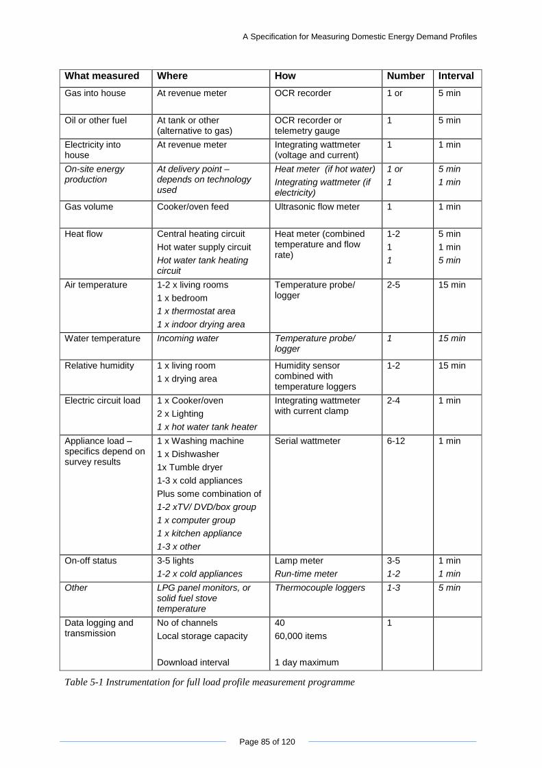
A Specification for Measuring Domestic Energy Demand Profiles
Page 85 of 120
What measured Where How Number Interval
Gas into house
At revenue meter OCR recorder 1 or 5 min
Oil or other fuel At tank or other (alternative to gas)
OCR recorder or telemetry gauge
1 5 min
Electricity into house
At revenue meter Integrating wattmeter (voltage and current)
1 1 min
On-site energy production
At delivery point – depends on technology used
Heat meter (if hot water)
Integrating wattmeter (if electricity)
1 or
1
5 min
1 min
Gas volume Cooker/oven feed Ultrasonic flow meter
1 1 min
Heat flow Central heating circuit
Hot water supply circuit
Hot water tank heating circuit
Heat meter (combined temperature and flow rate)
1-2
1
1
5 min
1 min
5 min
Air temperature 1-2 x living rooms
1 x bedroom
1 x thermostat area
1 x indoor drying area
Temperature probe/ logger
2-5 15 min
Water temperature
Incoming water Temperature probe/ logger
1 15 min
Relative humidity 1 x living room
1 x drying area
Humidity sensor combined with temperature loggers
1-2 15 min
Electric circuit load 1 x Cooker/oven
2 x Lighting
1 x hot water tank heater
Integrating wattmeter with current clamp
2-4 1 min
Appliance load – specifics depend on survey results
1 x Washing machine
1 x Dishwasher
1x Tumble dryer
1-3 x cold appliances
Plus some combination of
1-2 xTV/ DVD/box group
1 x computer group
1 x kitchen appliance
1-3 x other
Serial wattmeter 6-12 1 min
On-off status 3-5 lights
1-2 x cold appliances
Lamp meter
Run-time meter
3-5
1-2
1 min
1 min
Other LPG panel monitors, or solid fuel stove temperature
Thermocouple loggers 1-3 5 min
Data logging and transmission
No of channels
Local storage capacity
Download interval
40
60,000 items
1 day maximum
1
Table 5-1 Instrumentation for full load profile measurement programme
A Specification for Measuring Domestic Energy Demand Profiles
Page 86 of 120
specific household data collection plan is put together, and during which enough information is
collected to establish which category of user is involved, what appliances should be monitored,
and also to highlight any practical issues with locating sensors and data loggers. A second, more
detailed interview should be carried out after a plan has been established.
Survey questions need to be prepared in detail and tested out beforehand to make sure they are
clear while being worded tactfully – for example, household income appears to be a major driver
for energy use, but in British culture this is seen as asking very personal questions. It goes
without saying that there should be a clear explanation of the benefits of the exercise, and what
to expect, which need to be carefully prepared and rehearsed before contacting the volunteers.
The sheer quantity of data presents a challenge in itself: the database structure and the data
cleansing and quality control activities need to planned and tested in advance.
STARTUP PROCESS:
1a: Prepare speaker notes, Qs and As for interviewers, and survey questions; test with a friendly but not too closely involved group of ‘guinea pigs’.
1b: In parallel: Ask for volunteers; make initial visit to collect basic data and complete short survey, and establish what problems might occur when locating equipment in the house
2: Collect information on local population, housing, household size, energy use statistics; work out ideal stratification and sampling outcome work out what coverage of ideal the volunteers comprise;
3: If important strata are missing e.g. high consumers, look for more volunteers in target group
4: Decide specific measurement plan for each volunteer household; document
5a: Install and test meters, collect data on house construction
5b: In parallel: complete long survey on attitudes and use patterns
5c: In parallel: set up database
6: Test run of data collection and data cleansing for 1-2 weeks
5.6.2 Running and completing the data collection
During period of data collection some of the volunteers‟ circumstances may change: some will
move or lose interest, some will acquire new appliances, and others may interfere with appliance
meters. Meters or transmitters may fail. So there is a need to maintain relationships with the
volunteers in order to spot problems quickly and fix them if needed. The end of the exercise
presents an opportunity to say thank you, but also to learn from the experience for the future.
A Specification for Measuring Domestic Energy Demand Profiles
Page 87 of 120
COMPLETION PROCESS:
1: Debrief volunteers; check on what has changed since start, and when this happened; how they felt about living with instrumentation
2: Remove equipment,
3: Give some feedback on how it has gone and how this will benefit them/general knowledge
4: Use feedback to improve next round of data collection
5.7 Comparison with methodology used elsewhere
The proposed specification was compared against the methodology used in HEEP (Isaacs et al,
2010), REMODECE (2008) and the Swedish monitoring campaign (Zimmermann 2009).
The coverage of total energy inputs to the household – other than transport fuels for cars – was
attempted only by HEEP, the others looked at electricity only. In terms of end-use, the present
proposal uses the same level of breakdown as all three others. It does not cover individual
appliances to the same level of granularity as either REMODECE or the Swedish study, which
had a specific aim of gathering information to guide energy efficiency interventions with
appliance manufacturers. The proposed data set‟s usefulness would be restricted in this respect;
however, it was felt that if systematic appliance level data were to be added to the specification,
it would no longer meet the criterion of „reasonable incremental cost and effort‟.
Data resolution in this specification is higher than the 10-minute standard used in all three
comparators. This was deliberately done in order to ensure that the short period, high power
events that are of interest for supply-demand balancing, new technologies, and network analysis,
are picked up. The period for data collection is comparable to the detailed-level houses in HEEP
and the Swedish study, but much longer than REMODECE, this is because seasonal patterns for
end –uses other than heating and lighting are not well understood.
Compared to the other studies, more context data is collected than in any of the others, although
fewer specific questions are asked about appliance-level behaviours than in REMODECE.
Cost and effort reasons also dictated meant that the scope of temperature and RH measurements
in the specification is not wide enough to be able to use for validating complex thermodynamic
simulations. Similarly, no attempt was made to include time-use logging in the data collection
that could be used for occupant behaviour simulations.
A Specification for Measuring Domestic Energy Demand Profiles
Page 88 of 120
6 Observations of energy use in one house
A series of observations was made of the energy use patterns in one house where full knowledge
was available about the house, appliances and owner attitudes: that of the author. The aim was
to test the practical aspects of implementing the data collection plan in Chapter 5, and the factors
that might affect the interpretation of such data
6.1 Description
6.1.1 House and occupancy
The house is a ground floor conversion of an old Victorian mansion, with high ceilings and sash
windows. The main living rooms face south while the bedrooms are at the north-facing back
which is sheltered by an embankment and slope. Exterior and most interior walls are thick stone;
finishes vary from the original Victorian to new plasterboard with insulation. The windows have
been recently draught-proofed, with double glazing in two rooms. Under-floor insulation has
been installed in the living areas and some of the bedrooms.
The heating and hot water system is new, with a condensing combination boiler supplying two
separate heating circuits and all the hot water. The boiler has temperature compensated control
system; each heating circuit has its own thermostat, set at 18⁰ C in the bedroom area and 20⁰ C in
the living area; all the radiators have TRVs. Secondary heating includes a fan heater in the
bathroom, and a wood-burning stove in the living room.
There are normally two occupants who are in the house most of the day. However, frequent
resident visitors means that the average year-round occupancy is around 2.5. As many of these
are elderly or very young, the thermostats have to be set at 22⁰ C in the living area and 21⁰C in
the bedrooms for around 8 weeks in the year.
6.1.2 Instrumentation
Daily and hourly consumption were read from the revenue meters, whose required accuracy is
+2.5/-3.5% for electricity, +/-2% for gas (Ofgem, 2005). Other measurements were made with
cheap instruments designed for home use. Appliance power signatures were read with a Current
Cost Envi meter, which produces an instantaneous power reading every 6 seconds, based on a
current measurement to a precision of +/-50mA, and assuming nominal voltage of 240V. Given
the allowable range of voltages therefore the accuracy of the Envi power readings is estimated at
around +/-17% at the lowest recorded level of 125 W, and +/-7% in the upper range of
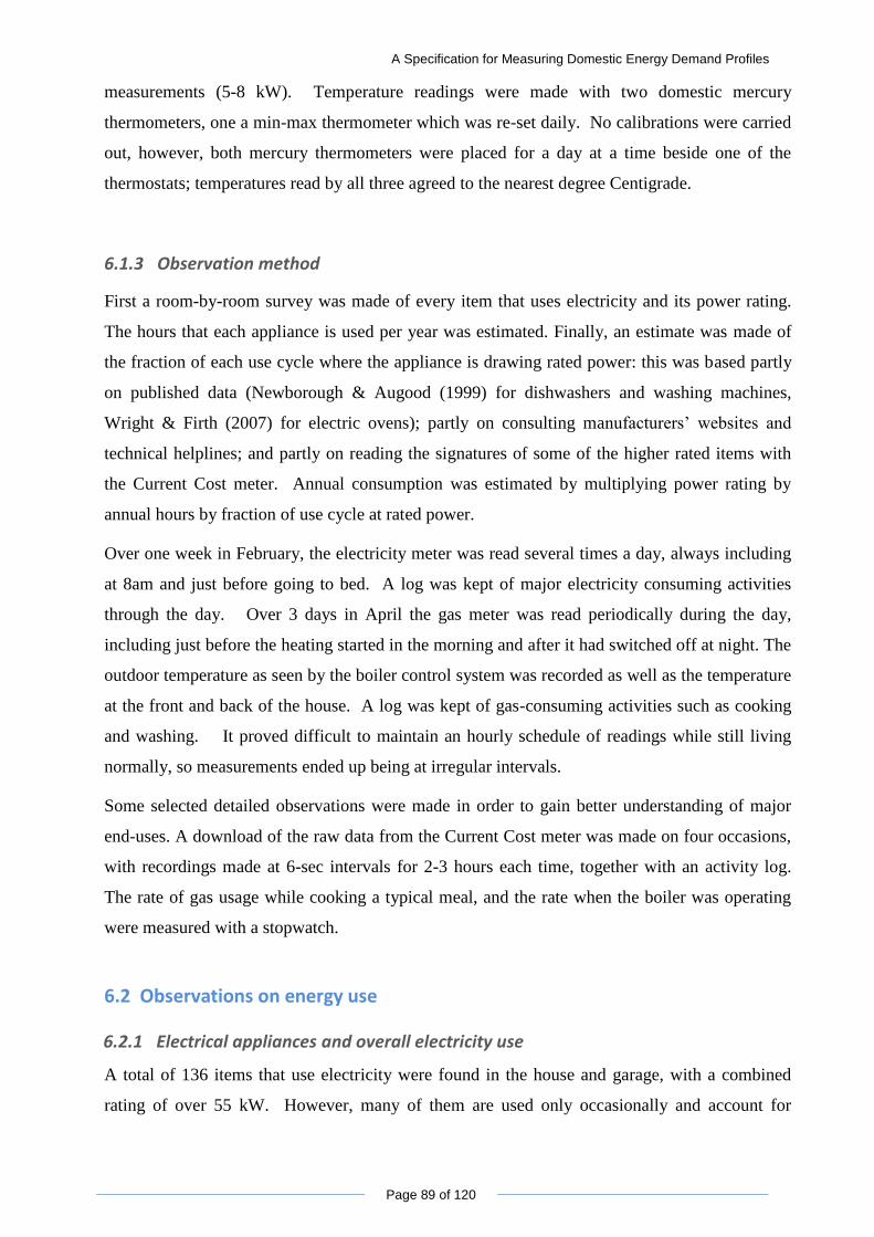
A Specification for Measuring Domestic Energy Demand Profiles
Page 89 of 120
measurements (5-8 kW). Temperature readings were made with two domestic mercury
thermometers, one a min-max thermometer which was re-set daily. No calibrations were carried
out, however, both mercury thermometers were placed for a day at a time beside one of the
thermostats; temperatures read by all three agreed to the nearest degree Centigrade.
6.1.3 Observation method
First a room-by-room survey was made of every item that uses electricity and its power rating.
The hours that each appliance is used per year was estimated. Finally, an estimate was made of
the fraction of each use cycle where the appliance is drawing rated power: this was based partly
on published data (Newborough & Augood (1999) for dishwashers and washing machines,
Wright & Firth (2007) for electric ovens); partly on consulting manufacturers‟ websites and
technical helplines; and partly on reading the signatures of some of the higher rated items with
the Current Cost meter. Annual consumption was estimated by multiplying power rating by
annual hours by fraction of use cycle at rated power.
Over one week in February, the electricity meter was read several times a day, always including
at 8am and just before going to bed. A log was kept of major electricity consuming activities
through the day. Over 3 days in April the gas meter was read periodically during the day,
including just before the heating started in the morning and after it had switched off at night. The
outdoor temperature as seen by the boiler control system was recorded as well as the temperature
at the front and back of the house. A log was kept of gas-consuming activities such as cooking
and washing. It proved difficult to maintain an hourly schedule of readings while still living
normally, so measurements ended up being at irregular intervals.
Some selected detailed observations were made in order to gain better understanding of major
end-uses. A download of the raw data from the Current Cost meter was made on four occasions,
with recordings made at 6-sec intervals for 2-3 hours each time, together with an activity log.
The rate of gas usage while cooking a typical meal, and the rate when the boiler was operating
were measured with a stopwatch.
6.2 Observations on energy use
6.2.1 Electrical appliances and overall electricity use
A total of 136 items that use electricity were found in the house and garage, with a combined
rating of over 55 kW. However, many of them are used only occasionally and account for
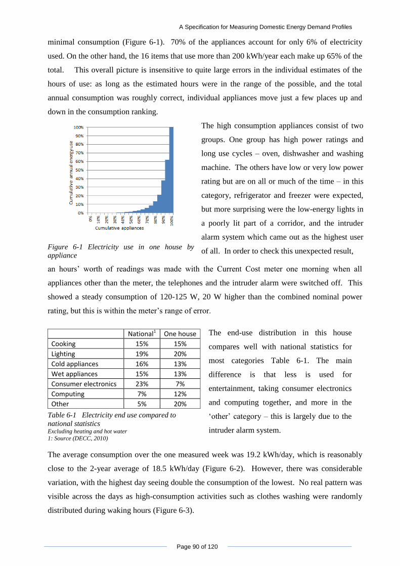
A Specification for Measuring Domestic Energy Demand Profiles
Page 90 of 120
minimal consumption (Figure 6-1). 70% of the appliances account for only 6% of electricity
used. On the other hand, the 16 items that use more than 200 kWh/year each make up 65% of the
total. This overall picture is insensitive to quite large errors in the individual estimates of the
hours of use: as long as the estimated hours were in the range of the possible, and the total
annual consumption was roughly correct, individual appliances move just a few places up and
down in the consumption ranking.
Figure 6-1 Electricity use in one house by
appliance
The high consumption appliances consist of two
groups. One group has high power ratings and
long use cycles – oven, dishwasher and washing
machine. The others have low or very low power
rating but are on all or much of the time – in this
category, refrigerator and freezer were expected,
but more surprising were the low-energy lights in
a poorly lit part of a corridor, and the intruder
alarm system which came out as the highest user
of all. In order to check this unexpected result,
an hours‟ worth of readings was made with the Current Cost meter one morning when all
appliances other than the meter, the telephones and the intruder alarm were switched off. This
showed a steady consumption of 120-125 W, 20 W higher than the combined nominal power
rating, but this is within the meter‟s range of error.
National1 One house
Cooking 15% 15%
Lighting 19% 20%
Cold appliances 16% 13%
Wet appliances 15% 13%
Consumer electronics 23% 7%
Computing 7% 12%
Other 5% 20%
Table 6-1 Electricity end use compared to
national statistics Excluding heating and hot water
1: Source (DECC, 2010)
The end-use distribution in this house
compares well with national statistics for
most categories Table 6-1. The main
difference is that less is used for
entertainment, taking consumer electronics
and computing together, and more in the
„other‟ category – this is largely due to the
intruder alarm system.
The average consumption over the one measured week was 19.2 kWh/day, which is reasonably
close to the 2-year average of 18.5 kWh/day (Figure 6-2). However, there was considerable
variation, with the highest day seeing double the consumption of the lowest. No real pattern was
visible across the days as high-consumption activities such as clothes washing were randomly
distributed during waking hours (Figure 6-3).
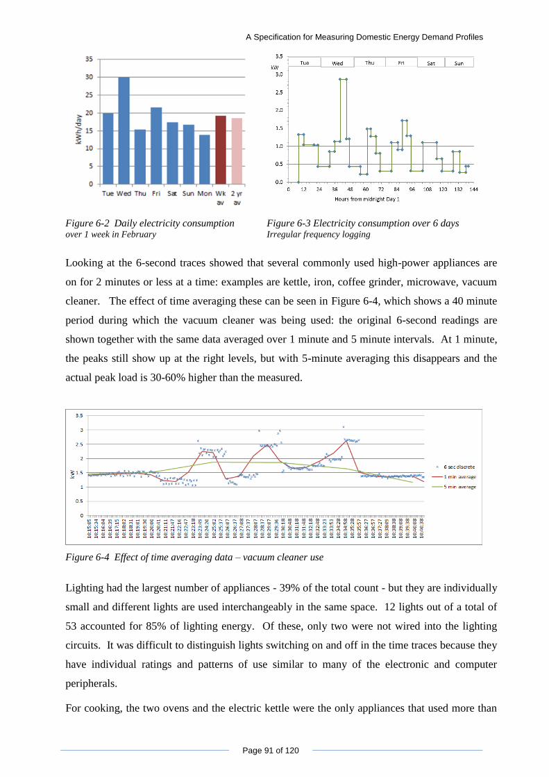
A Specification for Measuring Domestic Energy Demand Profiles
Page 91 of 120
Figure 6-2 Daily electricity consumption over 1 week in February
Figure 6-3 Electricity consumption over 6 days Irregular frequency logging
Looking at the 6-second traces showed that several commonly used high-power appliances are
on for 2 minutes or less at a time: examples are kettle, iron, coffee grinder, microwave, vacuum
cleaner. The effect of time averaging these can be seen in Figure 6-4, which shows a 40 minute
period during which the vacuum cleaner was being used: the original 6-second readings are
shown together with the same data averaged over 1 minute and 5 minute intervals. At 1 minute,
the peaks still show up at the right levels, but with 5-minute averaging this disappears and the
actual peak load is 30-60% higher than the measured.
Figure 6-4 Effect of time averaging data – vacuum cleaner use
Lighting had the largest number of appliances - 39% of the total count - but they are individually
small and different lights are used interchangeably in the same space. 12 lights out of a total of
53 accounted for 85% of lighting energy. Of these, only two were not wired into the lighting
circuits. It was difficult to distinguish lights switching on and off in the time traces because they
have individual ratings and patterns of use similar to many of the electronic and computer
peripherals.
For cooking, the two ovens and the electric kettle were the only appliances that used more than
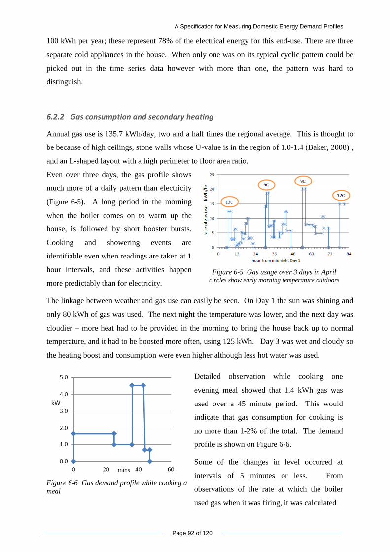
A Specification for Measuring Domestic Energy Demand Profiles
Page 92 of 120
100 kWh per year; these represent 78% of the electrical energy for this end-use. There are three
separate cold appliances in the house. When only one was on its typical cyclic pattern could be
picked out in the time series data however with more than one, the pattern was hard to
distinguish.
6.2.2 Gas consumption and secondary heating
Annual gas use is 135.7 kWh/day, two and a half times the regional average. This is thought to
be because of high ceilings, stone walls whose U-value is in the region of 1.0-1.4 (Baker, 2008) ,
and an L-shaped layout with a high perimeter to floor area ratio.
Even over three days, the gas profile shows
much more of a daily pattern than electricity
(Figure 6-5). A long period in the morning
when the boiler comes on to warm up the
house, is followed by short booster bursts.
Cooking and showering events are
identifiable even when readings are taken at 1
hour intervals, and these activities happen
more predictably than for electricity.
Figure 6-5 Gas usage over 3 days in April circles show early morning temperature outdoors
The linkage between weather and gas use can easily be seen. On Day 1 the sun was shining and
only 80 kWh of gas was used. The next night the temperature was lower, and the next day was
cloudier – more heat had to be provided in the morning to bring the house back up to normal
temperature, and it had to be boosted more often, using 125 kWh. Day 3 was wet and cloudy so
the heating boost and consumption were even higher although less hot water was used.
Figure 6-6 Gas demand profile while cooking a
meal
Detailed observation while cooking one
evening meal showed that 1.4 kWh gas was
used over a 45 minute period. This would
indicate that gas consumption for cooking is
no more than 1-2% of the total. The demand
profile is shown on Figure 6-6.
Some of the changes in level occurred at
intervals of 5 minutes or less. From
observations of the rate at which the boiler
used gas when it was firing, it was calculated
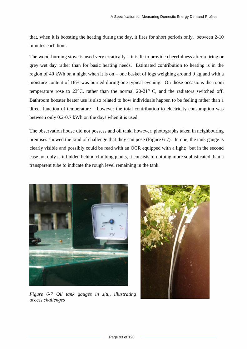
A Specification for Measuring Domestic Energy Demand Profiles
Page 93 of 120
that, when it is boosting the heating during the day, it fires for short periods only, between 2-10
minutes each hour.
The wood-burning stove is used very erratically – it is lit to provide cheerfulness after a tiring or
grey wet day rather than for basic heating needs. Estimated contribution to heating is in the
region of 40 kWh on a night when it is on – one basket of logs weighing around 9 kg and with a
moisture content of 18% was burned during one typical evening. On those occasions the room
temperature rose to 23⁰C, rather than the normal 20-21⁰ C, and the radiators switched off.
Bathroom booster heater use is also related to how individuals happen to be feeling rather than a
direct function of temperature – however the total contribution to electricity consumption was
between only 0.2-0.7 kWh on the days when it is used.
The observation house did not possess and oil tank, however, photographs taken in neighbouring
premises showed the kind of challenge that they can pose (Figure 6-7). In one, the tank gauge is
clearly visible and possibly could be read with an OCR equipped with a light; but in the second
case not only is it hidden behind climbing plants, it consists of nothing more sophisticated than a
transparent tube to indicate the rough level remaining in the tank.
Figure 6-7 Oil tank gauges in situ, illustrating
access challenges
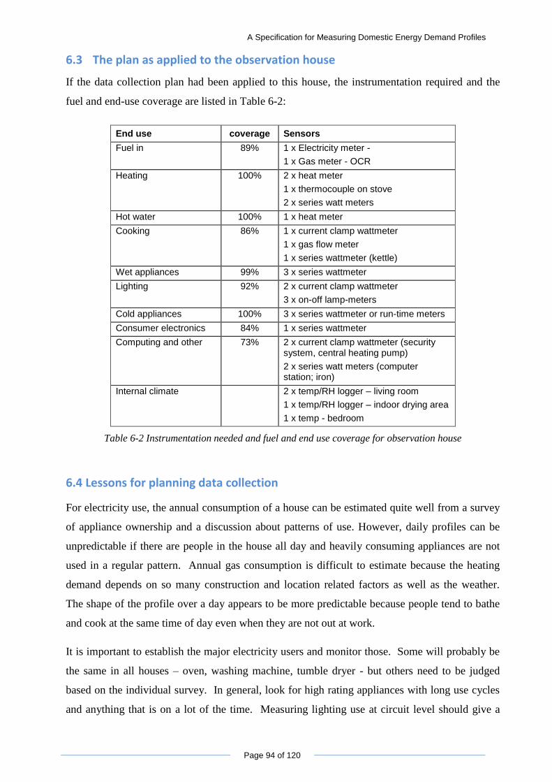
A Specification for Measuring Domestic Energy Demand Profiles
Page 94 of 120
6.3 The plan as applied to the observation house
If the data collection plan had been applied to this house, the instrumentation required and the
fuel and end-use coverage are listed in Table 6-2:
End use coverage Sensors
Fuel in 89% 1 x Electricity meter -
1 x Gas meter - OCR
Heating 100% 2 x heat meter
1 x thermocouple on stove
2 x series watt meters
Hot water 100% 1 x heat meter
Cooking 86% 1 x current clamp wattmeter
1 x gas flow meter
1 x series wattmeter (kettle)
Wet appliances 99% 3 x series wattmeter
Lighting 92% 2 x current clamp wattmeter
3 x on-off lamp-meters
Cold appliances 100% 3 x series wattmeter or run-time meters
Consumer electronics 84% 1 x series wattmeter
Computing and other 73% 2 x current clamp wattmeter (security system, central heating pump)
2 x series watt meters (computer station; iron)
Internal climate 2 x temp/RH logger – living room
1 x temp/RH logger – indoor drying area
1 x temp - bedroom
Table 6-2 Instrumentation needed and fuel and end use coverage for observation house
6.4 Lessons for planning data collection
For electricity use, the annual consumption of a house can be estimated quite well from a survey
of appliance ownership and a discussion about patterns of use. However, daily profiles can be
unpredictable if there are people in the house all day and heavily consuming appliances are not
used in a regular pattern. Annual gas consumption is difficult to estimate because the heating
demand depends on so many construction and location related factors as well as the weather.
The shape of the profile over a day appears to be more predictable because people tend to bathe
and cook at the same time of day even when they are not out at work.
It is important to establish the major electricity users and monitor those. Some will probably be
the same in all houses – oven, washing machine, tumble dryer - but others need to be judged
based on the individual survey. In general, look for high rating appliances with long use cycles
and anything that is on a lot of the time. Measuring lighting use at circuit level should give a

A Specification for Measuring Domestic Energy Demand Profiles
Page 95 of 120
good approximation to the total lighting load profile.
Data on house construction details is not easy to find. Changes made by successive owners are
not visible or known. There can be a lot of variation in different parts of old houses.
A resolution of one minute for electricity readings would have showed up the short duration
peaks recorded at 6-second intervals. Gas „events‟ such as boiler firing or adjusting the heat
when cooking can also occur on a time scale as short as 1-2 minutes.
Where secondary heating is used with central, it may be run more for comfort than for basic
heating, depending on how people are feeling rather than the temperature, so it does not conform
to a straightforward daily pattern. Energy used in secondary heating will not necessary translate
into the same energy use pattern if the fuel source is switched. However its use can make a big
difference to recorded temperatures.
Normal house occupancy can be altered if there are frequent visitors. This may be an important
factor in rural areas where many homes may do bed and breakfast business.
It is difficult to maintain a reliable time/ activity log. People are living lives and even with
highest possible motivation they will not always remember to update records.
A Specification for Measuring Domestic Energy Demand Profiles
Page 96 of 120
7 Conclusions
A need has emerged for good quality energy demand data on local patterns of energy
consumption for a whole host of purposes: to calibrate models; to allow scaling up of demand
profiles to a community level for supply-demand and network planning; to give a baseline
against which to track the effectiveness of specific energy saving initiatives; to investigate the
impact of shifts in fuel use for heating; and to quantify the extent of local opportunities for
demand management and smart appliance implementation.
Studies so far have demonstrated that predicting even current demand patterns is not
straightforward, especially in the domestic environment. Historically, domestic electricity
demand patterns were mainly looked at as statistical processes occurring in large groups, and it is
only relatively recently that investigations have started to be made into understanding what
drives consumption at a detailed level. Some of these measurement programmes have produced
seemingly contradictory results. Where clear trends have been noted, they are at a very high
level: when nights are longer, more electricity is used for lighting; if more people live in a house,
on average that house will use more electricity; if they have higher disposable incomes they will
be able to buy more and bigger appliances and therefore use more energy. However, every
measurement programme has found a very wide range of consumption among houses and
households that are apparently very similar. Household attitudes and habits appear to be the
most important factor that determines energy use and its daily pattern.
A major blocker to developing a consistent understanding is the fact that different data collection
programmes have measured different data sets, at different collection frequencies, and often just
for small or homogeneous groups of households and for total electricity use only. Source data is
generally not available, either because of commercial confidentiality, data privacy concerns or
simply because it has been lost. Translating findings from these projects to other parts of the
country requires making assumptions which may turn out to be inaccurate. The literature shows
that big differences in energy use exist between even neighbouring countries, so the assumption
that different parts of a single country as diverse in geography and population as the UK must be
open to question.
If future measurement programmes across different regions were to follow a consistent and
comprehensive measurement plan, and if the data were to be made available generally, this
would eventually build up to give better insights into what drives energy use and how this varies
by geography and over time. In the worst case, it would supply higher quality statistical data.
Using the insights gained from published measurement programmes, in conjunction with
A Specification for Measuring Domestic Energy Demand Profiles
Page 97 of 120
observations on one house, a data collection plan is proposed for this purpose. This involves
collecting around 40 sets of data per house, and measuring all fuel inputs as well as consumption
by each end use, with the highest priority given to end uses which might be subject to fuel
switching, demand-side management by time-shifting, or technology change. The data is
collected at the highest level of resolution needed to give a clear picture of short high-energy
events, 1 minute intervals for electricity and no more than 5 minutes for gas or heat flow. A
survey of the house and households involved is crucial for interpreting the data, and is most
effective when carried out face to face.
Most data collection programmes have a specific goal in mind, and this would go beyond the
needs of any individual investigation. However, much of the effort involved in any programme
is in setting it up, recruiting volunteers, and ensuring that clean data is being collected, so a
slightly larger data set should not require a huge incremental effort. Many practical difficulties
need to be overcome, particularly in finding an appropriate range of volunteers to represent both
the highest and lowest energy consumers in the area. Other challenges lie in in locating
equipment unobtrusively in the house, or in finding suitable monitoring equipment for difficult
places such as oil tanks. Privacy of personal data is extremely important.
However, one high-quality set of electricity demand data, accompanied by a household survey,
has now actually been put into the public domain, and shows that it is possible to include all the
useful context information without giving away information that could identify the participants.
It has been used for further analyses successfully, demonstrating the value that could be gained
from such data beyond the original purpose of the investigation.
7.1 Recommendations for further work
- Revise the wording of the survey questions to make them straightforward and non-
technical to users, while maintaining a „semi-structured‟ approach
- Investigate further whether there would be a benefit from collecting gas and heat flow
data at 1 minute rather than 5 minute intervals
- Extend the scope of the measurements to include domestic transport demand profiles, as
these will be increasingly important as electric cars start to become available. Possibly,
water use could also be included.
- Engage other researchers to support implementing a publicly available database – where
could this be held, ownership and maintenance
A Specification for Measuring Domestic Energy Demand Profiles
Page 98 of 120
References
Alfares, K. K., & Nazerruddin, M. (2002). Electric Load Forecasting: literature survey and
classification of methods. Int. J. Systems Science, 33, pp 23-34.
Bailey, J. (2000, December). Load profiling for retail choice: examining a complex and crucial
component of settlement. The Electricity Journal, 13(10), pp 69-74.
Baker, P. (2008). In situ U-value measurements in traditional buildings - preliminary results.
Retrieved May 20, 2011, from Historic Scotland: http://www.historic-
scotland.gov.uk/paul_baker_thermal_performance_of_traditional_masonry_walls.pdf
Bakker, V., Molderink, A., Hurink, L., & Smit, G. J. (2008). Domestic heat demand predictions
using neural networks. ISENG '08, Int. Conf. Systems Engineering pp. 189-194 Las Vegas:
IEEE.
Bladh, M., & Krantz, H. (2008). Towards a bright future? Household use of electric light: a
microlevel study. Energy Policy, 36, pp 3521-3530.
Boehme, T., Taylor, J., Wallace, R., & Bialek, J. (2006). Matching renewable electricity
generation with demand. University of Edinburgh.
Born, F. J., Clarke, J. A., & Johnstone, C. M. (2001a). Development and demonstartion of a
renewable energy based energy demand/supply decision support tool for the building design
profession. 7th International IBPSA Conference, pp 245-250. Rio de Janeiro, Brazil.
Born, F. J., Clarke, J. A., Johnstone, C. M., & Smith, N. A. (2001b). Merit - an evalution tool for
100% renewable energy provision. Renewable energy for islands conference. Chaira, Crete,
Greece.
Boyes, W. (2003). Instrumentation Reference Book, 3rd ed. Boston, Mass: Butterworth
Heinemann.
BP. (2009). Annual Report and Accounts - Refining and Marketing, Fuels Value Chains.
Brabec, M., Konar, O., Maly, M., Pelikan, E., & Vondracek, J. (2009). A statistical model for
natural gas standardized load profiles. Journal of the Royal Statistical Society, Series C, Applied
Statistics, 58, pp 123-139.
Brown, N., Wright, A. J., Shukla, A., & Stuart, G. (2010). Longitudinal analysis of energy
metering data from non-domestic buildings. Building Research and Information, 38, pp 80-91.
Burt, G. M., Elders, I. M., Galloway, S. T., Kelly, N. J., & Tumilty, R. M. (2008). Assessment of
highly distributed power systems using an integrated simulation approach. Proc IMechE Part
A: Power and Energy, 222, pp 657-668.
Chen, H., & Lee, W. L. (2010). Combined space cooling and water heating system for Hong Kong
residences. Energy and Buildings, 42, pp 243-250.
Chung, M., & Park, H.-C. (2010). Development of a software package for community energy
system assessment - part 1: Building a load estimator. Energy, 35, pp 2767-2776.
Clark, J. (2011, February). Introducing the Grid: Part Two. Scottish Renewables Grid Conference.
Glasgow.
Clarke, J. A. (2001). Energy simulation in building design, 2nd ed. Oxford: Butterworth
Heinemann.
Clarke, J., Hong, J., Kim, J. S., Hwang, I., & Lee, H. (2005). Simulation-based design procedure to
evaluate hybrid-renewable energy systems for residential buildings in Korea. Building
Simulation 2005, pp 191-197. Montreal, Canada.
Crosbie, T. (2008). Household energy consumption and consumer electronics: the case of
A Specification for Measuring Domestic Energy Demand Profiles
Page 99 of 120
television. Energy Policy, 36, pp 2191-2199.
Currie, R. A., Ault, G. W., & McDonald, J. R. (2006). Methodology for determination of
economic connection capacity for renewable generator connections to distribution networks
optimised by active power flow management. IEE Proc. Generation, Transmission and
Distribution, 153, pp 456-462.
Darby, S. J. (2011). Load management at home: advantages and drawbacks of some 'active
demand side' options. 2nd Int Conf on Microgneration and related technologies. Glasgow.
DECC. (2008). Middle Layer Super Output Area domestic electricity estimates. Retrieved April
21, 2011, from Sub-national energy consumption statistics:
http://www.decc.gov.uk/en/content/cms/statistics/regional/mlsoa_llsoa/mlsoa_llsoa.aspx
DECC. (2008). Middle Layer Super Output Area domestic gas estimates 2008. Retrieved April 21,
2011, from Sub-national energy consumption statistics:
http://wwwww.decc.gov.uk/en/content/cms/statistics/regional/mlsoa_llsoa/mlsoa_llsoa.aspx
DECC. (2009). Act on CO2 Calculator version 2.0: data, methodology and assumptions paper.
Retrieved May 25, 2011, from
http://www.decc.gov.uk/assets/decc/what%20we%20do/global%20climate%20change%20and
%20energy/tackling%20climate%20change/ind_com_action/calculator/1_20091120174357_e_
@@_actonco2calculatormethodology.pdf
DECC. (2010). Overall energy and domestic energy consumption Data Tables. Retrieved April 23,
2011, from Energy consumption in the United Kingdom:
http://www.decc.gov.uk/en/content/cms/statistics/publications/publications.aspx
Dept. Comm & Local Govt. (2011). Housing Statistics. Retrieved May 12, 2011, from
http://www.communities.gov.uk/housing/housingresearch/housingstatistics/housingstatisticsby/
Dept. Comm. & Local Govt. (2010). Table 406, Household Projections by District 1991-2033.
Retrieved May12 2011, from:
http://www.communities.gov.uk/housing/housingresearch/housingstatistics/housingstatisticsby/
householdestimates/livetables-households/
Elexon. (2011). Load Profiles and their use in electricity settlement.
Ellegard, K. (1999). A time-geographical approach to the study of everyday life of individuals - a
challenge of complexity. GeoJournal, 48, pp 167-175.
ENA. (2010). ENA Smart Metering System Use Cases. Electrical Networks Association.
Ferreira, V. G. (2009). The analysis of primary metered half-hourly electricty and gas consumption
in municipal buildings. PhD Thesis. Leicester: de Montfort University.
Firth, S. K., Buswell, R. A., & Lomas, K. J. (2009). A simple model of domestic PV systems and
their integration with building loads. Building Simulation, pp 789-796. Glasgow.
Firth, S., Lomas, K., Wright, A., & Wall, R. (2008). Indentifying trends in the use of domestic
appliances from household electricity consumption measurements. Energy and Buildings, 40,
pp 926-936.
Gill, Z. M., Tierney, M. J., Pegg, I. M., & Allan, N. (2011). Measured energy and water
performance of an aspiring low energy/carbon affordable housing site in the UK. Energy and
Buildings, 43, pp 117-125.
Gram-Hanssen, K. (2008). Consuming technologies - developing routines. J Cleaner Production,
16, pp 1181-89.
Hawkes, A. (2011). Marginal emissions rates in energy system change. 2nd Int. Conf. on
Microgeneration and related technologies. Glasgow.
A Specification for Measuring Domestic Energy Demand Profiles
Page 100 of 120
Hawkes, A., & Leach, M. (2005). Impacts of temporal precision in optimising modelling of micro-
CHP. Energy, 30, pp 1759-1779.
Hong, J., Kelly, N. J., Richardson, I., & Thomson, M. (2011). The influence of thermal storage on
microgeneration flexibility. Microgen II. Glasgow.
IBM. (2009). Lighting the way. Somers, NY: IBM Global Services.
Infield, D. G., Short, J., Horne, C., & Freris, L. L. (2007). Potential for domestic dynamic demand-
side management in the UK. Power Engineering Society General Meeting Tampa, Florida:
IEEE; pp 1-6
Isaacs, N., Camilleri, M., Burrough, L., Pollard, A., Saville-Smith, K., Fraser, R., et al. (2010).
Energy use in New Zealand households (Project HEEP). BRANZ.
Isaakson, C., & Karlsson, F. (2006). Indoor climate in low-energy houses - an interdisciplinary
investigation. Building and Environment, 41, pp 1678-1690.
Jacobson, A., Milman, A. D., & Kammen, D. M. (2005). Letting the (energy) Gini out of the
bottle: Lorenz curves of cumulative electricty consumption and Gini coefficients as metrics of
energy distribution and equity. Energy policy, 33, pp 1825-1832.
Jenkins, D. P., Tucker, R., & Rawlings, R. (2009). Modelling the carbon-saving performance of
domestic ground-source heat pumps. Energy and Buildings, 41, pp 587-595.
Lane, I. E., & Beute, N. (1996). A model of the domestic hot water load. IEEE Transactions on
Power Systems, 11, pp 1850-1854.
Leicester Energy Agency. (2010). AIM 4 SMEs Case Study #003: UK - Voluntary Action
Leicestershire (gas consumption).
McQueen, D. H., Hyland, P. R., & Watson, S. J. (2004). Monte Carlo simulation of residential
electricity demand for forecasting maximum demand on distribution networks. IEEE
Transactions on Power Systems, 19, pp 1685-1689.
National Grid. (2007). Gas Demand Forecasting Methodology.
Newborough, M., & Augood, P. (1999). Demand-side management opportunities for the UK
domestic sector. IEE Proceedings - Generation, Transmission and Distribution, 146, pp 283-
293.
Office for National Statistics. (2010). Household numbers and projections: Regional Trends 38.
Retrieved May 12, 2011, from Population estimates for UK, England and Wales, Scotland and
Northern Ireland: http://www.statistics.gov.uk/statbase/Product.asp?vlnk=15106
Ofgem. (2005). Gas and Electricity Meters Seminar. Retrieved May 19, 2011, from
http://webarchive.nationalarchives.gov.uk/+/http://www.ofgem.gov.uk/Networks/Techn/Metrol
gy/IndMeterng/In-servTest/Documents1/11010-In%20Service%20Seminar.pdf
Ofgem. (2010). Energy Demand Research Project (EDRP) Fifth Progress Report. Office of Gas
and Electricity Markets, London.
Ofgem. (2010, Aug). Revision of typical domestic consumption values. Retrieved May 21, 2011,
from Office of the Gas and Electricity Markets:
http://www.ofgem.gov.uk/Markets/RetMkts/Compl/Consumption/Documents1/Review%20of%
20typical%20domestic%20consumption%20values.pdf
Ofverholm, E. (2009). End Use Metering in the Residential Sector. Retrieved May 20, 2011,
energimyndigheten.se:http://www.energimyndigheten.se/Global/Engelska/Facts%20and%20fig
ures/Household%20electricity%20metering%20090203_E%20Ofverholm.pdf
Olofsson, T., Andersson, S., & Ostin, R. (1998). A method for predciting the annual building
A Specification for Measuring Domestic Energy Demand Profiles
Page 101 of 120
heating demand based on limited data. Energy and Buildings, 1998, pp 101-108.
ONS. (2009). Social Trends 39. Office for National Statistics.
Owen, P. (2006). The rise of the machines. Energy Saving Trust.
Paatero, J. V., & Lund, P. D. (2006). A model for generating household electricity load profiles.
Int. J. Energy Research, 30, pp 273-290.
Parker, D. S., Mazzara, M. D., & Sherwin, J. R. (1996). Monitored energy use patterns in low-
income housing in a hot and humid climate. Proc. 10th Symposium on Improving building
systems in hot and humid climates. Fort Worth, Texas.
Räsänen, T., Voukantsis, D., Niska, H., Karatzas, K., & Kolehmainen, M. (2010). Data-based
method for creating electricty use load profiles using large amounts of customer-specific hourly
measured electricty use data. Applied Energy, 87, pp 3538-3545.
REMODECE (2008). Residential Monitoring to Decrease Energy Use and Carbon Emissions in
Europe, Final Report, http://remodece.isr.uc.pt/
Richardson, I. (2010). Integrated high-resolution modelling of domestic electricity demand and
low voltage electricity distribution networks. PhD Thesis. Loughborough University.
Richardson, I. and Thomson, M., One-Minute Resolution Domestic Electricity Use Data, 2008-
2009 [computer file]. Colchester, Essex: UK Data Archive [distributor], October 2010. SN:
6583. Retrieved February 21, 2011, from Economic and Social Data Service:
http://www.esds.ac.uk/findingData/snDescription.asp?sn=6583
Richardson, I., Thomson, M., & Infield, D. (2008). A high-resolution domestic building occupancy
model for energy demand simulations. Energy and Buildings, 40, pp 1560-1566.
Richardson, I., Thomson, M., Infield, D., & Clifford, C. (2010). Domestic electricity use: a high-
resolution energy demand model. Energy and Buildings, 42, pp 1878-1887.
Richardson, I., Thomson, M., Infield, D., & Delahunty, A. (2009). A modelling framework for the
study of highly distributed power systems and demand side management. 1st Int Conf on
Sustainable Power Generation and Supply (SUPERGEN), pp 1-6). Nanjing, China.
Rijal, H. B., Tuohy, P., Humphrey, M. A., Nicol, J. F., A, S., & Clarke, J. A. (2007). Using resukts
from field surveys to predict the effect of open windows on thermal confort and energy use in
builidngs. Energy and Buildings, 39, pp 833-836.
Roaf, S., Nicol, F., Humphreys, M., Tuohy, P., & Boerstra, A. (2010). Twentieth century standards
for thermal comfort: promoting high energy buildings. Architectural Science Review, 53, pp 65-
77.
Schrock, D. (1997). Load Shape Development. Tulsa, Oklahoma: PennWell Publishing.
Shipworth, M., Firth, S. K., Gentry, M. I., Wright, A. J., Shipworth, D. T., & Lomas, K. J. (2010).
Central heating thermostat settings and timing: building demographics. Building Research and
Information, 38, pp 50-69.
Shorrock, J. I., & Utley, L. D. (2008). Domestic Energy Fact File. BRE Housing. DECC.
Smith, P., Husein, S., & Leonard, D. T. (1996). Forecasting short term regional gas demand using
an expert system. Expert Systems with Applications, 10, pp 265-273.
Stokes, M., Rylatt, M., & Lomas, K. (2004). A simple model of domestic lighting demand. Energy
and Buildings, 36, pp 103-116.
Strachan, P. A., Kokogiannakis, G., & Macdonald, I. A. (2006). History and development of
validation with the ESP-r simulation program. Building and Environment, 4, pp 601-609.
Strbac, G., Gan, C. K., Aunedi, M., Stanojevic, V., Djapic, P., Dejvises, J., et al. (2010). Benefits
A Specification for Measuring Domestic Energy Demand Profiles
Page 102 of 120
of Advanced Smart Metering for Demand Resopnse based Control of Distribution Networks:
Summary Report. SEDG/ Energy Networks Association.
Sulka, T., & Jenkins, N. (2008). Modelling of a housing estate with micro-combined heat and
power for power flow studies. Proc IMechE part A: Power and Energy, 222, pp 721-729.
Summerfield, A. J., Lowe, R. J., Bruhns, H. R., Caeiro, J. A., Steadman, J. P., & Oreszczyn, T.
(2007). Milton Keynes energy park revisited: changes in internal temperature and energy usage.
Energy and Buildings, 39, pp 783-791.
Summerfield, A. J., Pathan, A., Lowe, R. J., & Oreszczyn, T. (2010). Changes in energy demand
from lowenergy homes. Building Research and Information, 38, pp 42-49.
Tang, T., & Bhamra, T. A. (2008). Understanding consumer behaviour to reduce environmental
impacts through sustainable product design. Undisciplined! Proceedings of the Design
Research Society Conference, pp 183/1-183/15. Sheffield.
Thomson, M., & Infield, D. (2008). Modelling the impact of micro-CHP generators on electricty
distribution networks. Proc I MechE Part A: Power and Energy, 222, pp 697-706.
University of Strathclyde. (2009). Code of Practice on investigations involving human beings, 5th
ed. Glasgow.
Veitch, D. C., & Mahkamov, K. (2009). Assessement of economical and ecological benefits from
deployment of a domestic combined heat and power unit based on its experimental
performance. Proc I MechE Part A: Power and Energy, 223, pp 783-798.
Vuillecard, C; Hubert, C E; Contreau, R; Mazzenga, A; Stabat, P; Adnot, J, (2011). Small scale
impact of gas technologies on electric load management - µCHP & hybrid heat pump. Energy,
36, pp 2912-1923
Widen, J., & Wackelgard, E. (2010). A high-resolution stochastic model of domestic activity
patterns and electricity demand. Applied Energy, 87, pp 1880-1892.
Widen, J., Lundh, M., Vassileva, I., Dahlquist, E., Ellegard, K., & Wackelgard, E. (2009).
Constructing Constructing load profiles for household electricity and hot water from time use
data - Modelling approach and validation. Energy and Buildings, 41, pp 753-768.
Williamson, T. (2010). Comfort and energy use in five Australian award-winning houses:
regulated, measured and perceived. Building Research and Information, 38, pp 509-529.
Willis, H. L. (2004). Power Distribution Planning Reference Boook, 2nd ed. New York: Marcel
Dekker Inc.
Wright, A., & Firth, S. (2007). The nature of doestic electricity-loads and effects of time averaging
on statistics and on on-site generation calculations. Applied Energy, 84, pp 389-403.
Yao, R., & Steemers, K. (2005). A method of formulating energy load profile for domestic
buildings in the UK. Energy and Buildings, 37, pp 663-671.
Yohanis, Y. G., Mondol, J. D., Wright, A., & Norton, B. (2008). Real-life energy use in the UK:
How occupancy and dwelling characteristics affect domestic electricity use. Energy and
Buildings, 40, pp 1053-1059.
Yu, Z., Haghighat, F., Fung, B. C., & Yoshino, H. (2010). A decision tree method for building
energy demand modelling. Energy and Buildings, 42, pp1637-1646.
Zimmermann, J. P. (2009). End-use metering campaign in 400 households in Sweden. Swedish
Energy Agency.
A Specification for Measuring Domestic Energy Demand Profiles
Page 103 of 120
Appendix 1: Regional variations in domestic energy use - 2008
Fuel Mix1
Av electricity
per meter Ordinary tariff
Restricted tariff2
kWh pa
%
Restricted
tariff
meters2
Average gas
used per
meter3
kWh pa
Population:
Number
% working
age4,5,6
O: 3,784
R: 5,880
20% 16,907 59,623,200
62.0%
O: 3,752
R: 6,307
24% 18,043 5,194,000
62.6%
O: 3,281
R: 4,531
19% 15,004 588,470
67.4%
O: 4,043
R: 8,200
30% 19,991 90,040
58.6%
O: 4,382
R: 7,726
50% 0 22,210
61.0%
A Specification for Measuring Domestic Energy Demand Profiles
Page 104 of 120
Fuel Mix1
Av electricity
per meter Ordinary tariff
Restricted tariff2
kWh pa
%
Restricted
tariff
meters2
Average gas
used per
meter3
kWh pa
Population:
Number
% working
age4,5,6
O: 3,537
R: 4,887
44% 17,025 4,429,400
61.8%
O: 3,481
R: 4,671
50% 17,464 163,300
64.6%
Sources:
1. Energy Consumption in the UK, Overall & Domestic Data Tables (DECC, 2010)
2. Middle Layer Super Output Area (MLSOA) domestic electricity estimates (DECC, 2008)
3. Middle Layer Super Output Area (MLSOA) domestic gas estimates (DECC, 2008)
4. UK and regional: Population estimates for UK, England and Wales, Scotland and NI 2008
(Office for National Statistics, 2010)
5. Scotland Local Authority: Scottish Neighbourhood Statistics (Scottish Government, 2009)
6. England Local Authority: Department for Communities and Local Government: Housing -
Table 406 Household Projections by district 2008 (Dept. Comm. & Local Govt, 2010)
Page 105 of 120
Appendix 2: Summary of data sets reviewed
Source
Location, houses
Frequency,
Duration
Data collected Survey Not given or not
available
Summerfield et al,
2007
Milton Keynes
14 low energy
houses
Monthly /
10 mins, then
half hourly
15 months
Baseline
(1990): hourly
18 months
Gas, & electricity consumption /
Internal temperature – living
Internal temperature - bedroom
Relative humidity (max 10
separate loggers)
Baseline data as above, from 1990
study when houses newly built
Age and type of house, changes
to fabric since 1990
Heated floor area
No. of bedrooms
No and age of occupants
Household income
Appliance ownership
Primary heating and hot water
supply
Baseline: type and size of house
Occupancy pattern
Baseline: most survey
information missing
Summerfield et al,
2010
Milton Keynes
22 low energy
dwellings incl flats
Monthly
Baseline:
hourly
18 months
Gas & electricity consumption
Baseline: hourly energy
consumption only
Survey as above
Baseline: none available, but
floor area deduced
Internal temperature
Occupancy pattern
Shipworth et al,
2010
England and Wales
358 houses with
central heating
45 min
6 months
Living room and bedroom
temperature
External temperature
Type of house and year built
Insulation level and
draughtproofing, if known
Thermostat settings and active
hours
Household size and age
Electricity, gas or oil
usage
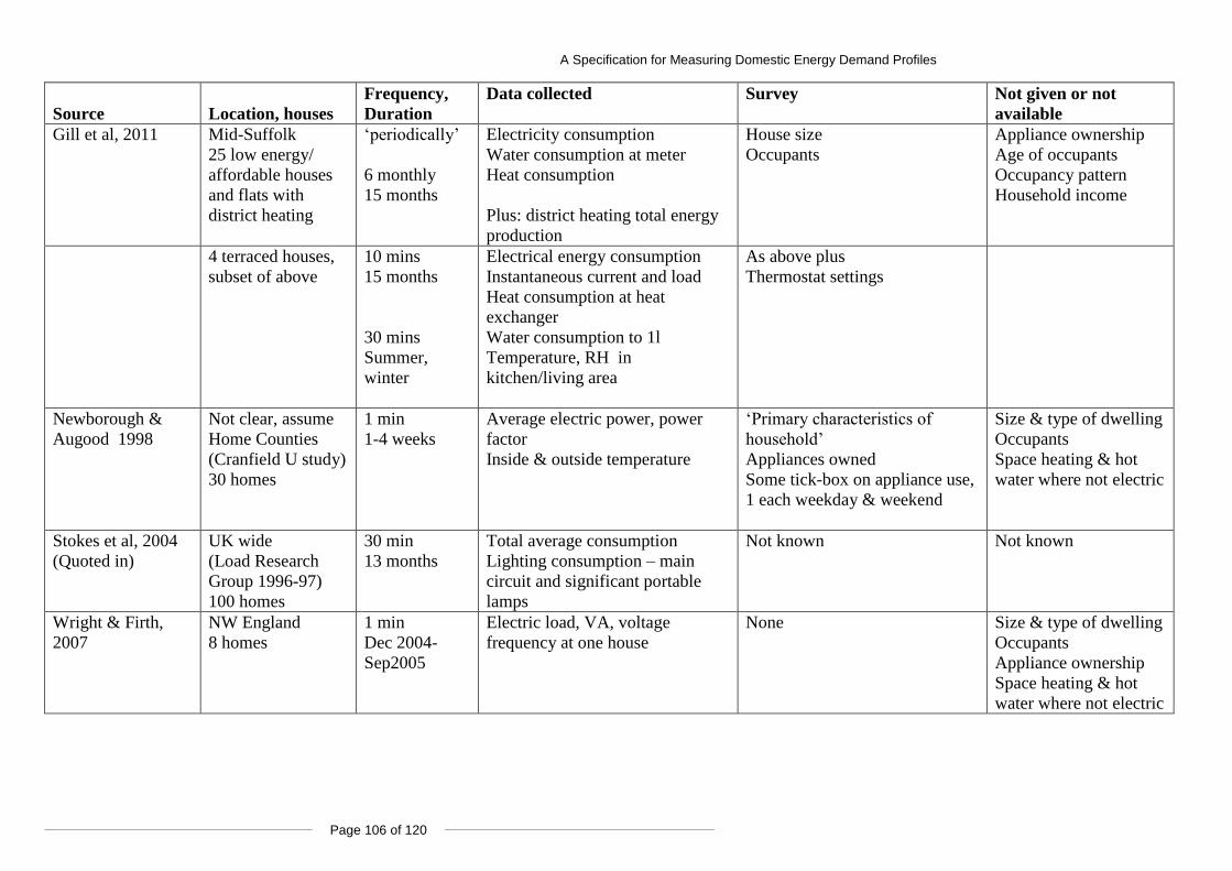
A Specification for Measuring Domestic Energy Demand Profiles
Page 106 of 120
Source
Location, houses
Frequency,
Duration
Data collected Survey Not given or not
available
Gill et al, 2011 Mid-Suffolk
25 low energy/
affordable houses
and flats with
district heating
„periodically‟
6 monthly
15 months
Electricity consumption
Water consumption at meter
Heat consumption
Plus: district heating total energy
production
House size
Occupants
Appliance ownership
Age of occupants
Occupancy pattern
Household income
4 terraced houses,
subset of above
10 mins
15 months
30 mins
Summer,
winter
Electrical energy consumption
Instantaneous current and load
Heat consumption at heat
exchanger
Water consumption to 1l
Temperature, RH in
kitchen/living area
As above plus
Thermostat settings
Newborough &
Augood 1998
Not clear, assume
Home Counties
(Cranfield U study)
30 homes
1 min
1-4 weeks
Average electric power, power
factor
Inside & outside temperature
„Primary characteristics of
household‟
Appliances owned
Some tick-box on appliance use,
1 each weekday & weekend
Size & type of dwelling
Occupants
Space heating & hot
water where not electric
Stokes et al, 2004
(Quoted in)
UK wide
(Load Research
Group 1996-97)
100 homes
30 min
13 months
Total average consumption
Lighting consumption – main
circuit and significant portable
lamps
Not known Not known
Wright & Firth,
2007
NW England
8 homes
1 min
Dec 2004-
Sep2005
Electric load, VA, voltage
frequency at one house
None Size & type of dwelling
Occupants
Appliance ownership
Space heating & hot
water where not electric
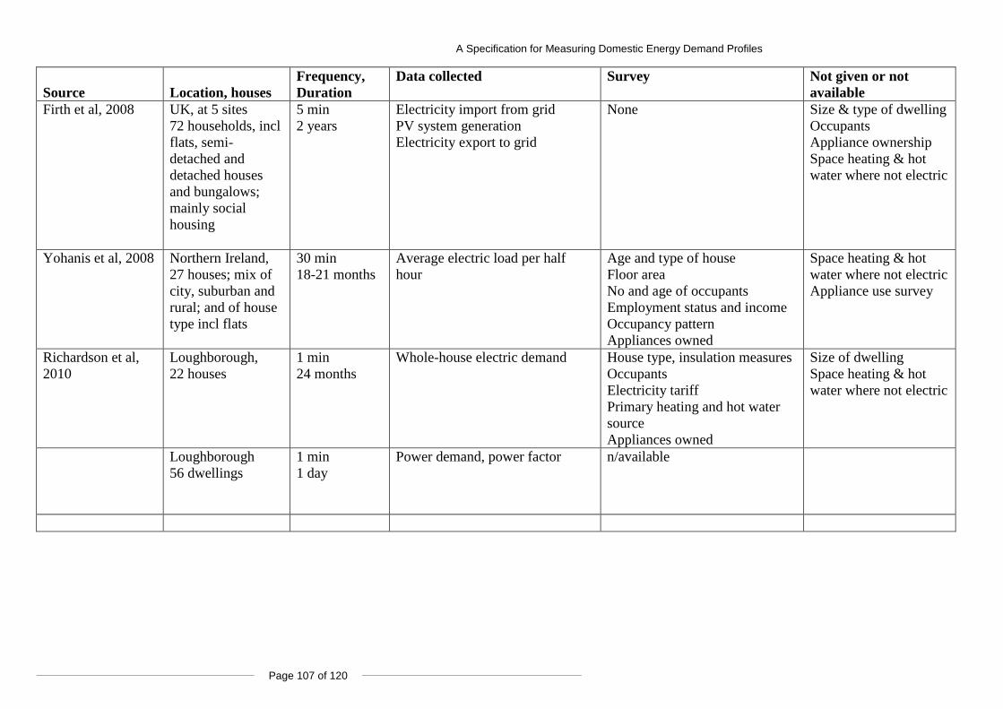
A Specification for Measuring Domestic Energy Demand Profiles
Page 107 of 120
Source
Location, houses
Frequency,
Duration
Data collected Survey Not given or not
available
Firth et al, 2008 UK, at 5 sites
72 households, incl
flats, semi-
detached and
detached houses
and bungalows;
mainly social
housing
5 min
2 years
Electricity import from grid
PV system generation
Electricity export to grid
None Size & type of dwelling
Occupants
Appliance ownership
Space heating & hot
water where not electric
Yohanis et al, 2008 Northern Ireland,
27 houses; mix of
city, suburban and
rural; and of house
type incl flats
30 min
18-21 months
Average electric load per half
hour
Age and type of house
Floor area
No and age of occupants
Employment status and income
Occupancy pattern
Appliances owned
Space heating & hot
water where not electric
Appliance use survey
Richardson et al,
2010
Loughborough,
22 houses
1 min
24 months
Whole-house electric demand House type, insulation measures
Occupants
Electricity tariff
Primary heating and hot water
source
Appliances owned
Size of dwelling
Space heating & hot
water where not electric
Loughborough
56 dwellings
1 min
1 day
Power demand, power factor
n/available
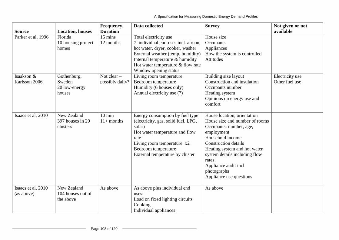
A Specification for Measuring Domestic Energy Demand Profiles
Page 108 of 120
Source
Location, houses
Frequency,
Duration
Data collected Survey Not given or not
available
Parker et al, 1996 Florida
10 housing project
homes
15 mins
12 months
Total electricity use
7 individual end-uses incl. aircon,
hot water, dryer, cooker, washer
External weather (temp, humidity)
Internal temperature & humidity
Hot water temperature & flow rate
Window opening status
House size
Occupants
Appliances
How the system is controlled
Attitudes
Isaakson &
Karlsson 2006
Gothenburg,
Sweden
20 low-energy
houses
Not clear –
possibly daily?
Living room temperature
Bedroom temperature
Humidity (6 houses only)
Annual electricity use (?)
Building size layout
Construction and insulation
Occupants number
Heating system
Opinions on energy use and
comfort
Electricity use
Other fuel use
Isaacs et al, 2010 New Zealand
397 houses in 29
clusters
10 min
11+ months
Energy consumption by fuel type
(electricity, gas, solid fuel, LPG,
solar)
Hot water temperature and flow
rate
Living room temperature x2
Bedroom temperature
External temperature by cluster
House location, orientation
House size and number of rooms
Occupants: number, age,
employment
Household income
Construction details
Heating system and hot water
system details including flow
rates
Appliance audit incl
photographs
Appliance use questions
Isaacs et al, 2010
(as above)
New Zealand
104 houses out of
the above
As above As above plus individual end
uses:
Load on fixed lighting circuits
Cooking
Individual appliances
As above
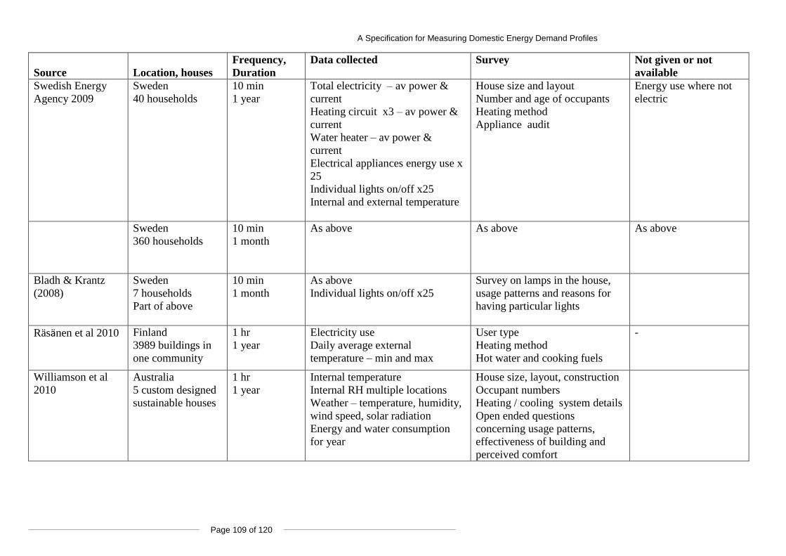
A Specification for Measuring Domestic Energy Demand Profiles
Page 109 of 120
Source
Location, houses
Frequency,
Duration
Data collected Survey Not given or not
available
Swedish Energy
Agency 2009
Sweden
40 households
10 min
1 year
Total electricity – av power &
current
Heating circuit x3 – av power &
current
Water heater – av power &
current
Electrical appliances energy use x
25
Individual lights on/off x25
Internal and external temperature
House size and layout
Number and age of occupants
Heating method
Appliance audit
Energy use where not
electric
Sweden
360 households
10 min
1 month
As above As above As above
Bladh & Krantz
(2008)
Sweden
7 households
Part of above
10 min
1 month
As above
Individual lights on/off x25
Survey on lamps in the house,
usage patterns and reasons for
having particular lights
Räsänen et al 2010 Finland
3989 buildings in
one community
1 hr
1 year
Electricity use
Daily average external
temperature – min and max
User type
Heating method
Hot water and cooking fuels
-
Williamson et al
2010
Australia
5 custom designed
sustainable houses
1 hr
1 year
Internal temperature
Internal RH multiple locations
Weather – temperature, humidity,
wind speed, solar radiation
Energy and water consumption
for year
House size, layout, construction
Occupant numbers
Heating / cooling system details
Open ended questions
concerning usage patterns,
effectiveness of building and
perceived comfort
A Specification for Measuring Domestic Energy Demand Profiles
Page 110 of 120
Appendix 3: Data collection plan
End use & Appliances
% of domestic
energy
total electricity
Contrib. to energy
use
Contrib. to peak
load
Potential for time
switching
Possible fuels
Influences on Consumption Measures – Input
Necessary/Optional
Measures – Output
Necessary/Optional
Space heating Central heating Open fireplaces Portable heaters Stoves Storage heaters Heat pumps Solar collector
58% 14% V High Yes Yes Gas – piped Gas - LPG Electricity
Oil Coal
Wood On-site generation
– hot water On-site generation
- electricity
House size & orientation
Immediate surroundings
House age, materials & insulation level -> U-values, thermal mass
Ventilation
Efficiency of heating system and controls
Weather/ time of year: temperature, sunlight, wind, RH
Casual gains from other appliances
Occupancy pattern –> # rooms heated over time
Attitude to energy use -> tariffs
Personal discomfort level – what is ‘too cold/hot’ (may vary with age/life stage) -> thermostat settings , changes, overrides
Primary fuel input – all fuels
Heat input (appliance dependent)
If liquid CH: gas or oil usage; heating circuit temperature and flow rate
If fixed or portable electric or storage heaters: appliance load(s)
If fixed or portable gas: gas flow rate(s)
If solid: quantity used log, moisture content; stove temperature
If on-site generation: electricity or heat input from device
Secondary heating fuel input, if appropriate
Air temperature – bedroom
Air temperature – living room(s)
Air temperature – by thermostat
RH – living room
RH – kitchen, bathroom
Air temperature - hall
Floor temperature –living room(s)
Window open status - living room
A Specification for Measuring Domestic Energy Demand Profiles
Page 111 of 120
End use & Appliances
% of domestic
energy
total electricity
Contrib. to energy
use
Contrib. to peak
load
Potential for time
switching
Possible fuels
Influences on Consumption Measures – Input
Necessary/Optional
Measures – Output
Necessary/Optional
Space heating (cont)
Survey:
General surroundings and orientation of house
Layout, number of living and bedrooms
Floor area, ceiling height, window size
External wall, floor, and roof materials, insulation level
Primary and secondary heating fuels
Last year’s heating & electricity usage from bills
On-site generation, if any
Number of occupants, age, occupancy pattern incl. visitors/vacation use
Survey:
Comfort perceptions: temperature in different rooms, stuffiness, draughtiness, problem areas
Pattern of use in rooms – e.g. teenage children use bedrooms as living rooms
Control system and thermostat settings, thermostat location – awareness, how often changed,
Pattern of secondary heating use
Views on heating costs – degree of knowledge, degree of concern
Hot water Hot water tanks Back boilers Combi boilers Instant boilers
23% 14% High Possible Yes From heating system
Direct
Gas - piped
Electricity
On-site generation – hot water
No. of occupants
Type of appliance e.g. power shower
Incoming water temperature
Personal preference – frequency, timing, length of shower, depth of bath…
Whether dishwasher and washing machine have hot or cold water feeds
Hot water fuel usage
If tank: Hot water tank output temperature and flow rate
If combi or instant: heater output temperature and flow rate (s)
Incoming water temperature
Survey:
Hot water system and types of appliances
Dishwasher and washing machine feeds
Survey:
General household patterns – baths vs showers, evenings vs mornings
Time use diary
A Specification for Measuring Domestic Energy Demand Profiles
Page 112 of 120
End use & Appliances
% of domestic
energy
total electricity
Contrib. to energy
use
Contrib. to peak
load
Potential for time
switching
Possible fuels
Influences on Consumption Measures – Input
Necessary/Optional
Measures – Output
Necessary/Optional
Cooking Hobs, Ovens, Kettles, Microwaves, Slow cookers, Breadmakers,
4% 11% High Yes No Gas Electricity
LPG Wood Coal
Household size, age/ life stage
Personal preference – cooking vs heating ready-made meals, enjoys cooking or not, family meals or individual
Type of appliance & rating
Cooking fuel usage
If electric cooker: load on hob/oven circuit
If gas: flow rate to cooker Other appliance consumption e.g. kettle, depending on use pattern
Survey:
Type of hob, type and number of ovens
Ownership of various kitchen appliances
Survey:
General household patterns – family or individual meals, enjoyment of cooking
Number of hours a week spent cooking
Kettle filled each time or just enough for number of cups
Kitchen appliances/ gadgets used most frequently
Time use diary
A Specification for Measuring Domestic Energy Demand Profiles
Page 113 of 120
End use & Appliances
% of domestic
energy
total electricity
Contrib. to energy
use
Contrib. to peak
load
Potential for time
switching
Possible fuels
Influences on Consumption Measures – Input
Necessary/Optional
Measures – Output
Necessary/Optional
Consumer electronics TV, Set top box, Games console, set top box, Power supplies, speakers…
4% 16% Med Possible No Electricity Number and type of appliances esp TVs
Occupancy pattern
Personal preference – use of free time, family vs individual use, other sources of entertainment by time of year
Attitude to use – switching off, leaving on standby, leaving on when not in room
Consumption of appliance group(s) e.g. TV/set top box/DVD
On-off state of TV(s)
Total electricity - overnight steady load for standby use
Survey:
Number of TVs, type: CRT/plasma/LCD/LED and size
Other related appliances e.g. speakers, set top box, DVD, games console,
Survey:
Pattern of use of TV and associated appliances – one or several on at one time,
Average hours each TV is watched
Time use diary
Lighting Standard, Halogen, Fluorescent, ESB, LED Indoor, outdoor
3% 13% Med Yes No Electricity Number, type and rating of lights/lumieres
Time of year and climate -> ambient light levels
Occupancy pattern
Attitude to use – lights switched off when room unoccupied or not
Lighting circuit(s) consumption
Individual light on/off state, for important fixtures
Survey:
Number of lights in house, grouping in areas such as living room or hall
Where & how many low –energy lights, fluorescent lights
In a typical evening, how many lights on through the house
Plugged in lamps most often used, morning and evening - power
Number of outdoor lights, and whether on timer or manual switch
Light level in living room
Light level in study
Light level in kitchen
Survey:
Comfort perceptions on light levels through the day – any areas where light is generally on
A Specification for Measuring Domestic Energy Demand Profiles
Page 114 of 120
End use & Appliances
% of domestic
energy
total electricity
Contrib. to energy
use
Contrib. to peak
load
Potential for time
switching
Possible fuels
Influences on Consumption Measures – Input
Necessary/Optional
Measures – Output
Necessary/Optional
Cold appliances Freezer, Refrigerator, Fridge-freezer, Drinks chiller
3% 12% Yes No Yes Electricity Number and energy consumption rating of appliances
Location – e.g. next to cooker or in cool utility room
Attitude to use – temperature setting, opening frequency, leaving door open when filling shelves
Individual appliance consumption
Total electricity - overnight cyclical load
Survey:
Number of fridges, freezers, chillers; where located
Are age and energy rating known
Wet appliances Washing machine, Tumble dryer, Washer –dryer, Dishwasher
3% 11% High Possible Yes Electricity Number and energy consumption rating of appliances
Hot or cold water intake of appliances
Incoming water temperature
Occupancy pattern
Electricity tariff
Weather / time of year -> outdoor or indoor drying
Household size and life stage
Attitude to use – frequency and temperature setting of loads, flexibility to use off-peak tariff if exists
Individual or grouped appliance consumption
Incoming water temperature
Survey:
Number of appliances
Number of times a week each is used
Temperature and cycle used
Temperature and RH in normal indoor drying area
Time use diary
Survey:
Preferences for dishwashing – by hand or machine all the time
Preferences for drying – indoor, outdoor, machine
Timing of when machines run – random or planned
A Specification for Measuring Domestic Energy Demand Profiles
Page 115 of 120
End use & Appliances
% of domestic
energy
total electricity
Contrib. to energy
use
Contrib. to peak
load
Potential for time
switching
Possible fuels
Influences on Consumption Measures – Input
Necessary/Optional
Measures – Output
Necessary/Optional
Computing Desktop, Laptop, Monitor, Printer, Speakers, Scanners
1.2% 5%
Low No No Electricity Number and energy consumption of appliances
Working from home pattern
Occupancy pattern
Attitude to use – switching off vs standby
Consumption of appliance group e.g. computer/monitor/printer
Survey:
Number of computers
Number of associated peripherals each has
Survey:
Pattern of use of computer and associated appliances – one or several on at one time,
Average hours each computer is switched on, and average hours actively sued
Time use diary
Other Vacuum cleaners, Personal products, Power tools, Garden tools, Security systems, Hot tubs, Saunas, Water beds
0.9% 4% Possible No Some Electricity mainly But possible
alternatives e.g. portable gas
Number and energy consumption rating of appliances
Occupancy pattern
Attitude to use – switching off vs standby
Individual appliance consumption, if large (e.g. hot tub)
Security system - part of overnight base consumption
Survey:
Ownership of other large consuming appliances e.g. sauna, hot tub, security system; and their power rating and frequency of use
A Specification for Measuring Domestic Energy Demand Profiles
Page 116 of 120
Appendix 4: Loughborough 1-minute resolution electricity demand data
ORDINARY TARIFF H6 H3 H9 H15 H11 H10 H22 H20 H14 H19
2008 CONSUMPTION
Average kW 0.24 0.26 0.32 0.38 0.38 0.40 0.46 0.52 0.58 0.69
Max kW 7.86 14.25 6.43 8.26 6.75 10.15 8.30 11.15 19.68 9.88
% missing data 6% 6% 14% 4% 10% 23% 5% 6% 0% 2%
kWh per day 5.7 6.1 7.7 9.1 9.1 9.6 11.0 12.5 14.0 16.5
Annual kWh 2076 2248 2835 3346 3349 3501 4021 4570 5127 6044
2009 CONSUMPTION
Average kW 0.27 0.29 0.35 0.35 0.39 0.36 0.49 0.63 0.51 0.54
Max kW 7.27 12.48 5.92 7.93 6.86 8.02 7.72 11.40 17.97 8.26
% missing data 25% 87% 77% 16% 38% 38% 29% 17% 11% 16%
kWh per day 6.5 6.9 8.3 8.5 9.3 8.5 11.8 15.2 12.2 13.0
Annual 2385 2534 3023 3098 3408 3114 4295 5540 4462 4730
Elexon Stratum Low Low Low Mid Mid Mid Mid Mid Mid Mid
Ofgem band 1 2 2 3 3 3 3 3 4 4
SURVEY RESULTS
Type of dwelling semi semi terr det det det terr semi semi semi
Occupants 2008 1 2 n/a 4 4 4 3 5 6 n/a
Occupants 2009 2 2 3 3 2 4 3 5 5 4
Timers n n n y y n y n n n
Central Heating y y y y y y y y y y
Electric Heating n n n n n n n n n n
Electric water heating all yr winter all yr all yr all yr all yr all yr winter all yr winter
Insulation types (4 max) 3 3 2 3 4 4 3 3 1 3
% Low Energy bulbs 50% 100% 60% 50% 80% 40% 80% 99% 30% 25%
A Specification for Measuring Domestic Energy Demand Profiles
Page 117 of 120
ORDINARY TARIFF H6 H3 H9 H15 H11 H10 H22 H20 H14 H19
Electric Shower 0 1 0 0 0 0 0 1 1 0
Floodlights 1 0 0 1 0 1 1 0 1 1
Cold appliances 1 2 1 1 2 2 3 1 1 2
Electric hob 0 0 0 1 0 0 0 0 0 0
Electric oven 0 1 0 1 0 1 0 1 1 1
Washing machine/wd 1 1 1 1 1 1 1 1 1 1
Tumble drier 0 0 0 1 0 1 1 0 0 1
Dishwasher 0 1 0 1 0 1 1 1 1 1
TV 1 2 1 5 1 1 1 1 1 4
Computers 1 3 1 3 2 2 2 1 4 3
No of people 1 2 3 4 4 4 3 5 6 4
kWh/person, 2008 2076 1124 945 836 837 875 1340 914 854 1511
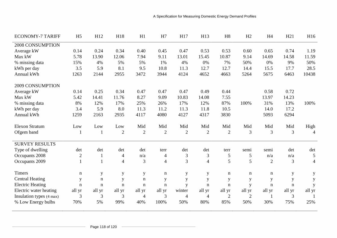
A Specification for Measuring Domestic Energy Demand Profiles
Page 118 of 120
ECONOMY-7 TARIFF H5 H12 H18 H1 H7 H17 H13 H8 H2 H4 H21 H16
2008 CONSUMPTION
Average kW 0.14 0.24 0.34 0.40 0.45 0.47 0.53 0.53 0.60 0.65 0.74 1.19
Max kW 5.78 13.90 12.06 7.94 9.11 13.01 15.45 10.87 9.14 14.69 14.58 11.59
% missing data 15% 4% 5% 5% 1% 4% 0% 7% 50% 0% 9% 50%
kWh per day 3.5 5.9 8.1 9.5 10.8 11.3 12.7 12.7 14.4 15.5 17.7 28.5
Annual kWh 1263 2144 2955 3472 3944 4124 4652 4663 5264 5675 6463 10438
2009 CONSUMPTION
Average kW 0.14 0.25 0.34 0.47 0.47 0.47 0.49 0.44 0.58 0.72
Max kW 5.42 14.41 11.76 8.27 9.09 10.83 14.08 7.55 13.97 14.23
% missing data 8% 12% 17% 25% 26% 17% 12% 87% 100% 31% 13% 100%
kWh per day 3.4 5.9 8.0 11.3 11.2 11.3 11.8 10.5 14.0 17.2
Annual kWh 1259 2163 2935 4117 4080 4127 4317 3830 5093 6294
Elexon Stratum Low Low Low Mid Mid Mid Mid Mid Mid Mid Mid High
Ofgem band 1 1 2 2 2 2 2 2 3 3 3 4
SURVEY RESULTS
Type of dwelling det det det det terr det det terr semi semi det det
Occupants 2008 2 1 4 n/a 4 3 3 5 5 n/a n/a 5
Occupants 2009 1 1 4 3 4 3 4 5 5 2 3 4
Timers n y y y n y y n n n y y
Central Heating y n y n y y y y y y y y
Electric Heating n n n n n y n n y n n y
Electric water heating all yr all yr all yr all yr all yr winter all yr all yr all yr all yr all yr all yr
Insulation types (4 max) 3 3 3 4 3 4 4 2 2 1 3 1
% Low Energy bulbs 70% 5% 99% 40% 100% 50% 80% 85% 50% 30% 75% 25%
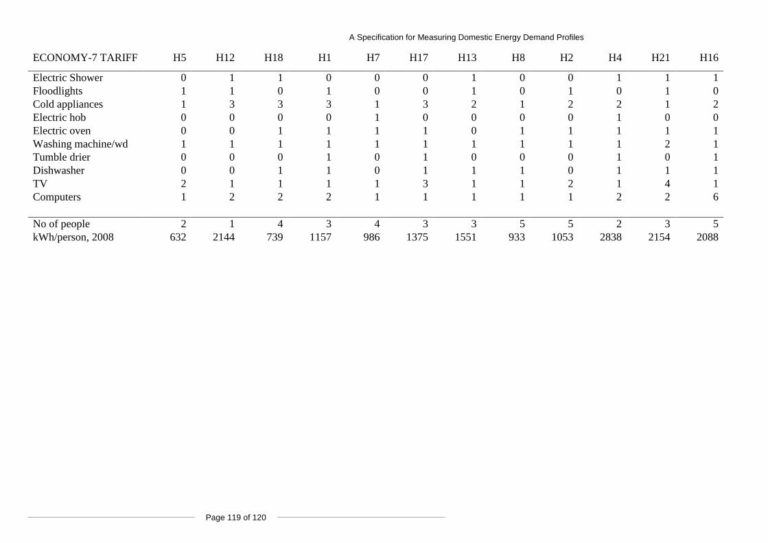
A Specification for Measuring Domestic Energy Demand Profiles
Page 119 of 120
ECONOMY-7 TARIFF H5 H12 H18 H1 H7 H17 H13 H8 H2 H4 H21 H16
Electric Shower 0 1 1 0 0 0 1 0 0 1 1 1
Floodlights 1 1 0 1 0 0 1 0 1 0 1 0
Cold appliances 1 3 3 3 1 3 2 1 2 2 1 2
Electric hob 0 0 0 0 1 0 0 0 0 1 0 0
Electric oven 0 0 1 1 1 1 0 1 1 1 1 1
Washing machine/wd 1 1 1 1 1 1 1 1 1 1 2 1
Tumble drier 0 0 0 1 0 1 0 0 0 1 0 1
Dishwasher 0 0 1 1 0 1 1 1 0 1 1 1
TV 2 1 1 1 1 3 1 1 2 1 4 1
Computers 1 2 2 2 1 1 1 1 1 2 2 6
No of people 2 1 4 3 4 3 3 5 5 2 3 5
kWh/person, 2008 632 2144 739 1157 986 1375 1551 933 1053 2838 2154 2088

Page 120 of 120