A SPATIAL COMPLEX ANALYSIS OF AGGLOMERATION

AND SETTLEMENT PATTERNS

Peter Nijkamp

February 1978

Research Memoranda are interim reports on research being conducted by the International Institute for Applied Systems Analysis, and as such receive only limited scientific review. Views or opinions contained herein do not necessarily represent those of the Institute or of the National Member Organizations supporting the Institute.

Copyright @ 1978 IIASA

All rights reserved. No part of this publication may be reproduced or transmitted in any form or by any means, electronic or mechanical, including photocopy, recording, or any information storage or retrieval system, without permission in writing from the publisher.

Preface

This paper is an outgrowth of the author's lecture delivered at IIASA in September 1977. The lecture was jointly organized by Integrated Regional Development Task and Human Settlement Systems Task, both of which are sharing the common research interests in the analytical methods, planning means and policy implementation insttuments with respect to spatial allocation- interaction of activities in a functionally integrated economic and social subsystem.

This paper presents a new analytical technique concerning the internal and external agglomeration economies which have become increasingly significant to spatial issues. It also intends to provide a reasonable background for a better under- standing of the characteristics of changes actually taking place in spatial systems. Therefore, it will serve as a com- plementary output to the results stemmin~ from the research activities of both Tasks which will be carried out at IIASA.

The author is Professor of Regional Economics at the Free University, Amsterdam. He has published numerous articles and books in the fields of programming theory, entropy models, en- vironmental problems and multi-criteria decision-making.

- iii -

This paper was o r i g i n a l l y prepared under t h e t i t l e "Modelling f o r Management" f o r p r e s e n t a t i o n a t a Nate r Research Cent re (U.K. ) Conference on "River P o l l u t i o n Con t ro l " , Oxford, 9 - 1 1 A s r i l , 1979.

A b s t r a c t

T r a d i t i o n a l l o c a t i o n t h e o r y and modern s p a t i a l i n t e r a c t i o n t h e o r y a r e i m p o r t a n t b u t n o n e t h e l e s s u n s a t i s f a c t o r y t o o l s t o a n a l y z e t h e d e t e r m i n a n t s of s p a t i a l agg lomera t ion p a t t e r n s .

E f f i c i e n c y p r i n c i p l e s and o r g a n i z a t i o n a l p r i n c i p l e s do n o t p r o v i d e a s u f f i c i e n t l y broad framework f o r an a n a l y s i s o f human s e t t l e m e n t sys tems , a s w i l l be i l l u s t r a t e d by means o f s e v e r a l examples ( compara t ive -cos t a n a l y s i s , i n d u s t r i a l complex a n a l y s i s , a t t r a c t i o n a n a l y s i s , e t c . ) .

There fo re it i s wor thwi le t o e x p l o r e new ways of t h i n k i n g . S p a t i a l complex a n a l y s i s may be a u s e f u l approach t o p r o v i d e an i n t e g r a t e d view of t h e agglomerat ion phenomena i n h e r e n t i n human s e t t l e m e n t p a t t e r n s . By means o f v e c t o r p r o f i l e methods a q u a n t i t a t i v e frame of r e f e r e n c e can be p rov ided f o r a f u r t h e r s t u d y o f t h e d e t e r m i n a n t s and t h e coherence of a c e r t a i n agglomerat ion p a t t e r n .

The u s e of a newly developed m u l t i v a r i a t e s t a t i s t i c a l t e c h n i q u e , v i z in te rdependence a n a l y s i s , p r o v i d e s a r e a s o n a b l e background f o r a more profound a n a l y s i s based on s p a t i a l correspondence t e c h n i q u e s . Given t h i s t e c h n i q u e , t h e de te rmi - n a n t s of a c e r t a i n s p a t i a l a l l o c a t i o n p a t t e r n can be i d e n t i f i e d .

The a n a l y s i s w i l l be i l l u s t r a t e d by means of s e v e r a l e m p i r i c a l r e s u l t s f o r t h e p r o v i n c e of North-Holland i n t h e Ne the r lands .

F i n a l l y , t h e a t t e n t i o n w i l l be focused on an i n t e g r a t i o n of t h e f o r e g o i n g approach w i t h s p a t i a l p r o c e s s e s , w h i l e urban and p h y s i c a l p l a n n i n g a s p e c t s w i l l a l s o he d i s c u s s e d .

A Spatial Complex Analysis of Agglomeration

and Settlement Patterns

1. INTRODUCTION

In the post-war period industrial location patterns and

human settlement systems have been characterized by rapid

changes. Urbanization and spatial agglomeration were a first

major trend, followed by a large-scale suburbanization move-

ment and urban decay in a broader sense. At the moment a more

diffuse pattern arises: on the one hand, the suburbanization

movement appears to continue as a movement toward rural and

even peripheral areas, while on the other hand some big cities

tend to start again acting as an engine of new agglomeration

forces. Problems of an optimal city size, but even more im-

portant: of an optimal spatial lay-out, are becoming increas-

ingly important. Operational insight into the various forces

determining the development of location patterns and human

sett:err.ents is still lacking. Can traditional location theory

serve to fill this gap in our knowledge?

Location theory is usually considered as a core theory

of regional economics and economic geography. The determinants

of location behavior of housel~olds and firms have been studied

at length in the past (see for a survey inter alia Carlino

[I9771 and Paelinck and Nijkamp [1976]).

From the seventies onwards, however, the focus of regional

economists and geographers has been shifted gradually from

location analysis per se to spatial interaction analysis. In

the latter analysis the attention for the determinants of geo-

graphical associations of economic activities has been

substituted for a closer examination of spatial mobility patterns

associated with a given location pattern of human settlement

systems (df. the popularity of entropy naxinizing models-or

gravity-type models, and of spatial allocation models).

During the last years, however, it has become increasingly

evident that the overwhelming amount of literature in the field

of spatial interaction analysis has sometimes tended to neglect

the intricate interrelationship between spatial structure and

spatial interaction. Especially the determinants of urban agglom-

eration forces appear to deserve more attention due to the negative

externalities of urban growth processes. The development of

urban systems can, however, hardly be explained by means of

traditional location analysis. Therefore, a broader view of

urban phenomena seems to be necessary, in which the spatial,

social and economic aspects of urban systems are integrated.

In this paper a brief survey of some recently developed

spatial agglomeration theories will be presented. Then the

notion of a spatial complex analysis will be introduced,

followed by an exposition of this type of analysis on the basis

of spatial activity profiles.

Spatial complex analysis will be used by its nature in this

paper to investigate in an operational sense the main charac-

teristics and determinants of spatial activity and interaction

patterns of human settlement systems. The multivariate nature

of spatial complex analysis will be studied by means of a

rather new statistical techniqce, viz interdependence analysis. --

This analysis will be set out in more detail in this paper.

Finally, the use of interdependence analysis in the framework

of spatial complex analysis will be illustrated by means of

a numerical application to one of the Dutch provinces, viz

North-Holland. Both the data base and the various results

achieved will be discussed, followed by an evaluation of the

methodology employed, an outline of further research and a

discussion of some policy implications.

2. AGGLOMERATION ANALYSIS

The theoretical underpinnings of traditional location

and agglomeration theory were mainly provided by the Weberian

approach based on a cost minimizing behavior of private firns

taking into account the spatially dispersed locations of inputs

and outputs as well as the benefits from a joint spatial

juxtaposition of firms. The latter agglomerative economies from

the point of view of both entrepreneurs and households were

studied extensively in the Christaller-Ldsch framework, while

the study of spatial associations between economic activities

was stimulated from the fifties onwards especially by Isard

[1956].

In the post-war period, agglomeration economies have mainly

been studied from the point of view of entrepreneurial behavior.

Firms acting on a private land use market were supposed to

determine for a major part the land use and location pattern of

a society. The locational decisions of private households and

of public agencies and even the whole human settlement system

were frequently regarded as a derivative of private locational

behavior of entrepreneurs based on micro- or macro-economic

efficiency principles.

Examples of this approach are inter alia the comparative-

cost analysis, the industrial complex analysis and its related

growth pole theory, and the attraction theory.

The comparative cost analysis (see Isard et al. [1959]) is

essentially a cost-effectiveness approach based on a detailed

calculation of all private costs involved in constructing an

integrated complex of economic activities at a certain place.

An evaluation of alternative configurations (i.e., activities)

of this complex takes place on the basis of a comparative frame

of reference for costs of an already existing complex.

The industrial complex analysis as well as the growth pole

theory are based on savings on transportation and production

costs due to a spatial concentration of industries (~zamanski

and Czamanski [1976], Nijkamp [1972], Richter [I9691 and Streit

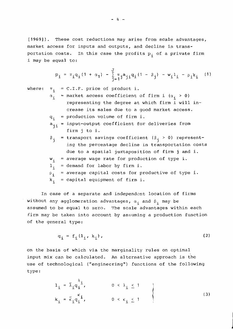
[ 1 9 6 9 ] ) . These cos t r e d u c t i o n s may a r i s e f rom scale a d v a n t a g e s ,

m a r k e t a c c e s s f o r i n p u t s and o u t p u t s , and d e c l i n e i n t r a n s -

p o r t a t i o n c o s t s . I n t h i s case t h e p r o f i t s pi of a p r i v a t e f i r m

i may b e e q u a l t o :

where: = C . I . F . p r i c e of p r o d u c t i. i

a = marke t access c o e f f i c i e n t of f i r m i ( a > 0 ) i i r e p r e s e n t i n g t h e d e g r e e a t which f i r m i w i l l i n -

crease i t s sales due t o a good marke t a c c e s s .

q i = p r o d u c t i o n volume o f f i r m i .

a = i n p u t - o u t p u t c o e f f i c i e n t f o r d e l i v e r i e s from j i f i r m j t o i.

i = t r a n s p o r t s a v i n g s c o e f f i c i e n t ( B i > 0 ) r e p r e s e n t - J J

i n g t h e F e r c e n t a g e d e c l i n e i n t r a n s p o r t a t i o n cos ts

due t o a s p a t i a l j u x t a p o s i t i o n o f f i r m j and i.

w = a v e r a g e wage r a t e f o r p r o d u c t i o n o f t y p e i. i

li = demand f o r l a b o r by f i r m i.

= a v e r a g e c a p i t a l c o s t s f o r p r o d u c t i v e o f t y p e i.

ki = c a p i t a l equipment o f f i r m i.

I n c a s e o f a s e p a r a t e and i n d e p e n d e n t l o c a t i o n o f f i r m s

w i t h o u t any a g g l o m e r a t i o n a d v a n t a g e s , a i and Bi may be

assumed t o be e q u a l t o z e r o . The s c a l e a d v a n t a g e s w i t h i n e a c h

f i r m may b e t a k e n i n t o a c c o u n t by assuming a p r o d u c t i o n f u n c t i o n

of t h e g e n e r a l t y p e :

on t h e b a s i s o f which v i a t h e m a r g i n a l i t y r u l e s on o p t i m a l

i n p u t mix can b e c a l c u l a t e d . An a l t e r n a t i v e approach i s t h e

u s e of t e c h n o l o g i c a l ( " e n g i n e e r i n g " ) f u n c t i o n s o f t h e f o l l o w i n g

t y p e :

where and K are constant coefficients. Relationships ( 1 ) through (3) contain all the elements

of agglomeration economics distinguished by Hoover [1948], viz

scale advantages (internal to the firm), localization advantages

(external to the firm but internal to the industry concerned)

and urbanization economies (external to the firm and external

to the industry). These types of models can be used in a

combinational planning framework, in which different sets of

industrial activities are to be evaluated against each other

(see, for example Albegov [I9721 and Nijkamp [19721).

Relationships (1) to 63) may be used to calculate the

gain in private efficiency due to a spatial concentration of

economic activities. In the growth pole theory these efficiency

gains have been assumed to stimulate a wide-spread process of

economic growth. In this theory the agglomeration benefits are

considered as the source of a spatial diffusion of economic

growth.

It should be noted that these benefits were only calculated

in aggregate terms, while the distributional implications of

such a growth process were mainly left aside. It should also be

added that a precise computation of the order of magnitude of

agglomeration benefits is very difficult due to la.ck of infor-

mation and of a standard of reference (Van Delft and

Nijkamp 119771).

Another method for studying spatial association between

economic activities at a sectoral level is the attraction

theory (Klaassen [I 9761 and Van Wickeren [1 9721 ) . The

strength of attraction theory is that it attempts to use

communication costs inherent to demand and supply relations for

interindustrial deliveries from an input-output table as a

basis for assessing the relative spatial attraction power of a

certain industry.

In addition to efficiency principles as an explanatory

device for geographical associations of firms, organizational

principles may be assumed as well (a survey can be found in

Hamilton [19741). The idea underlying the organizational

principle is that especially large-scale plants need an indus-

trial framework with a spatial access to and a geographical

association with other firms. These factors are sometimes hard

to quantify, but by means of multi-attribute methods applied to

interview data a quantitative analysis is in principle possible

(Keeble [19691).

The organizational and the efficiency principle provide an

explanatory basis for a spatial concentration of activities and

for the presence of agglomeration economics. Beside explanatory

theories, in the past much attention has been paid to the

calculation of measures for spatial concentrations between

activities. These measures were mainly based on economic linkages

such as intermediate and final deliveries of a firm within a

certain area (Britton [1969] , Czannnski [I9721 , Goddard [1973], Hoare [1975], Latha~r. [1976] and McCarty et al. [I9561 j . Especially the correlation coefficients between employment

data of manufacturing industries in the same area have frequently

been used as a measure of geographic-economic linkage. A good

example of the latter type of analysis applied to an enormous

data base for the U.S. is contained in Latham [19761.

In the case of a large number of activites an analysis of

the associated correlation matrix is rather time-consuming,

so that the principal comnonent techniques can be used to

reduce the data base (see among others Bergsman et al. [19721,

Van Holst and Molle [1 9771 , and Roepke et al. [1 9741 . It is

clear, however, that the use of principal component techniques

gives rise to additional problems such as the lack of a

theoretically-based explanation of the results of this statis-

tical procedure.

In addition to explanatory and descriptive devices an

alternative approach to urban agglomeration analyses may be found

by means of a general urban production function (see inter alia

Carlino [I 9771 , Isard [1 9561 and Kawashima [1 9751 ) . The

underlying idea is that the externalities of urban size may lead

to productivity increases in the city, until beyond a certain

city size negative externalities are coming about (caused by

population density, congestion, decline in quality of life, etc.).

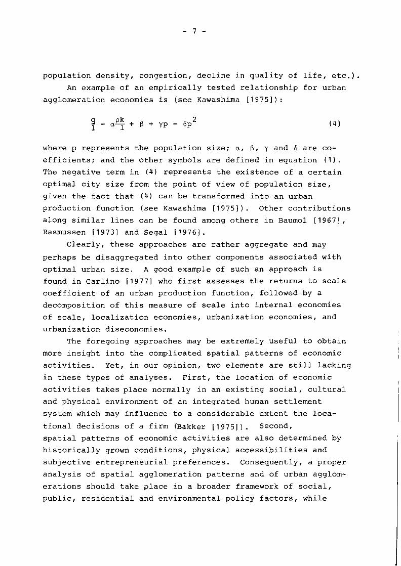
An example of an empirically tested relationship for urban

agglomeration economies is (see Kawashima [I97511 :

where p represents the population size; a, 6, y and 6 are co-

efficients; and the other symbols are defined in equation (1).

The negative term in (4) represents the existence of a certain

optimal city size from the point of view of population size,

given the fact that ( 4 ) can be transformed into an urban

production function (see Kawashima [1975]). Other contributions

along similar lines can be found among others in Baumol [1967],

Rasmussen [ 19731 and Segal [1976] . Clearly, these approaches are rather aggregate and may

perhaps be disaggregated into other components associated with

optimal urban size. A good example of such an approach is

found in Carlino [I9771 who' first assesses the returns to scale

coefficient of an urban production function, followed by a

decomposition of this measure of scale into internal economies

of scale, localization economies, urbanization economies, and

urbanization diseconomies.

The foregoing approaches may be extremely useful to obtain

more insight into the complicated spatial patterns of economic

activities. Yet, in our opinion, two elements are still lacking

in these types of analyses. First, the location of economic

activities takes place normally in an existing social, cultural

and physical environment of an integrated human settlement

system which may influence to a considerable extent the loca-

tional decisions of a firm (~akker [I 9751 ) . Second,

spatial patterns of economic activities are also determined by

historically grown conditions, physical accessibilities and

subjective entrepreneurial preferences. Consequently, a proper

analysis of spatial agglomeration patterns and of urban agglom-

erations should take place in a broader framework of social,

public, residential and environmental policy factors, while

also the dynamics of spatial location patterns have to be taken

into account.

These elements bring us to the notion of a spatial complex

analysis as a generalization of an industrial complex to indicate

that an existing spatial agglomeration pattern cannot be

properly understood via the restricted concepts of industrial

complexes or spatial economic associations, but have to be

placed in a broader framework of spatial integrations of

socio-economic, cultural, physical and public amenities. A

spatial complex can be conceived of as a coherent set of diverse

human activities with a high degree of interaction and located

in the same region. The notion of a spatial complex analysis

indicates that the explanation of a certain spatial lay-out

cannot be based on a single efficiency criterion, but on a

wide variety of determinants of spatial behavior and of a

human settlement pattern. This will be discussed more thoroughly

in the next section.

3. SPATIAL ACTIVITY PROFILES

Suppose an area subdivided into a set of regions (r = 1 ,

..., R). Suppose also a set of economic sectors (s = 1 , ..., S) and a set of indicators k characterizing the spatial complex at

hand (k = 1 , ..., K). Then the question arises: how can the

regional differences between the diverse sectors and between

the complex indicators be explained? Which determinants are

especially responsible for a certain spatial agglomeration

pattern?

The answer to these questions requires a systematic

analysis of the spatial complex pattern concerned. An

operational tool for representing a certain spatial lay-out

in a quantitative manner is the use of a spatial activity

profile. A spatial activity profile is a multidimensional

(vector) representation of the elements or activities character-

izing the spatial pattern (concentration, association, etc.) of

a certain region. Needless to say that such a spatial activity

profile should not only relate to economic activities but to

a broader set of variables (like public facilities) pertaining

t o t h e s p e c i a l complex of t h e region concerned.

The elements c h a r a c t e r i z i n g a s p a t i a l complex may be

d i s t i n g u i s h e d i n t o i n d i v i d u a l and r e l a t i o n a l elements. I nd iv idua l

elements a r e s e p a r a t e elements p e r t a i n i n g t o a p roper ty of a

c e r t a i n economic s e c t o r o r of a human se t t l emen t p a t t e r n wi thout

any r e l a t i o n t o o t h e r s e c t o r s ( f o r example, employment p e r

s e c t o r , popula t ion d e n s i t y , e t c . ) . R e l a t i o n a l elements p e r t a i n

t o l i nkages wi th o t h e r s e c t o r s o r wi th a human s e t t l e m e n t system

( f o r example, t h e degree of i n t e r s e c t o r a l i n t e r a c t i o n , o r t h e

s e c t o r a l degree of f i n a l demand o r i e n t a t i o n ) .

C l e a r l y , t h e r e l a t i o n a l elements of a c e r t a i n s p a t i a l

complex a r e e s p e c i a l l y l i nked t o s p a t i a l agglomeration p a t t e r n s ,

s o t h a t t h e s e elements r e f l e c t mainly l o c a l i z a t i o n and urbani-

z a t i o n economies.

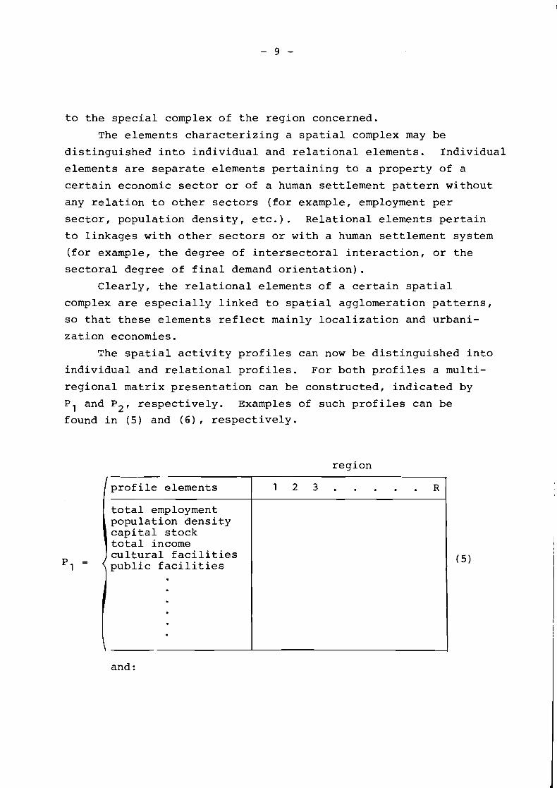
The s p a t i a l a c t i v i t y p r o f i l e s can now be d i s t i n g u i s h e d i n t o

i n d i v i d u a l and r e l a t i o n a l p r o f i l e s . For both p r o f i l e s a mul t i -

r eg iona l mat r ix p r e s e n t a t i o n can be cons t ruc t ed , i n d i c a t e d by

P I and P 2 , r e s p e c t i v e l y . Examples of such p r o f i l e s can be

found i n (5 ) and ( 6 ) , r e s p e c t i v e l y .

reg ion

and :

p r o f i l e elements

t o t a l employment popula t ion d e n s i t y c a p i t a l s tock t o t a l income c u l t u r a l f a c i l i t i e s p u b l i c f a c i l i t i e s

1 2 3 . . . . . R

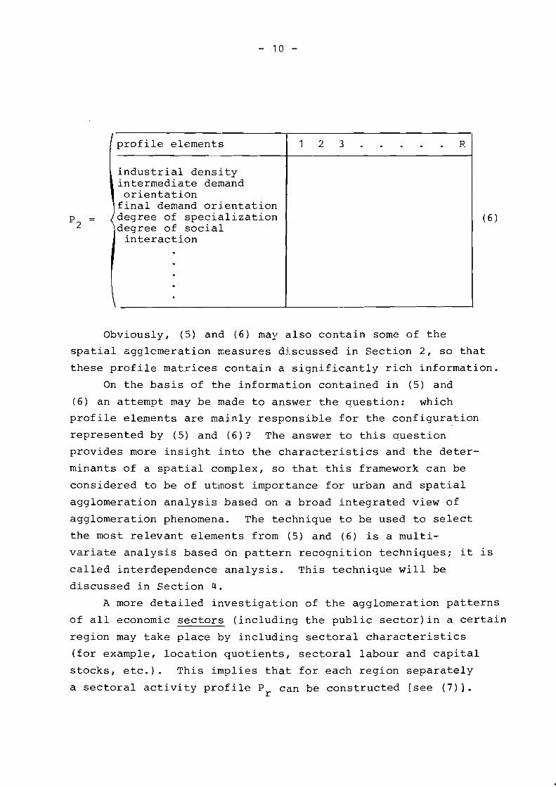
Obviously, (5) and (6) may also contain some of the

/profile elements

industrial density intermediate demand orientation final demand orientation degree of specialization degree of social interaction

I

\

spatial agglcmeration rceasures discussed in Section 2, so that

these profile matrices contain a significantly rich information.

On the basis of the information contained in (5) and

1 2 3 . . . . . F.

(6) an attempt may be made to answer the question: which

profile elements are mainly responsible for the configuration

represented by (5) and (6)? The answer to this question

provides more insight into the characteristics and the deter-

minants of a spatial complex, so that this framework can be

considered to be of utmost importance for urban and spatial

agglomeration analysis based on a broad integrated view of

agglomeration phenomena. The technique to be used to select

the most relevant elements from (5) and (6) is a multi-

variate analysis based on pattern recognition techniques; it is

called interdependence analysis. This technique will be

discussed in Section 4.

A more detailed investigation of the agglomeration patterns

of all economic sectors (including the public sector)in a certain

region may take place by including sectoral characteristics

(for example, location quotients, sectoral labour and capital

stocks, etc.). This implies that for each region separately

a sectoral activity profile Pr can be constructed [see ( 7 ) l .

Iprofile elements 1 2 3 . . . . . . S

location quotient volume of labor capital stock spatial externalities

\

It is clear that (7) can again be distinguished into

individual and relational profiles, so that various measures

for the degree of spatial association (for example, input-output

linkages) can be included in (7). The regional activity

profile represented by (7) iay provide more insight into the

main determinants of the sectoral location pattern for each

region separately. Here again the same technique, viz inter-

dependence analysis, may be used.

An alternative approach may be to create a sectoral activity

profile, in which the profile elements are linked to the various

regions involved. In this case the characteristics of footloose

industries, labor- and input-oriented industries or market-

oriented industries can be studied in more detail.

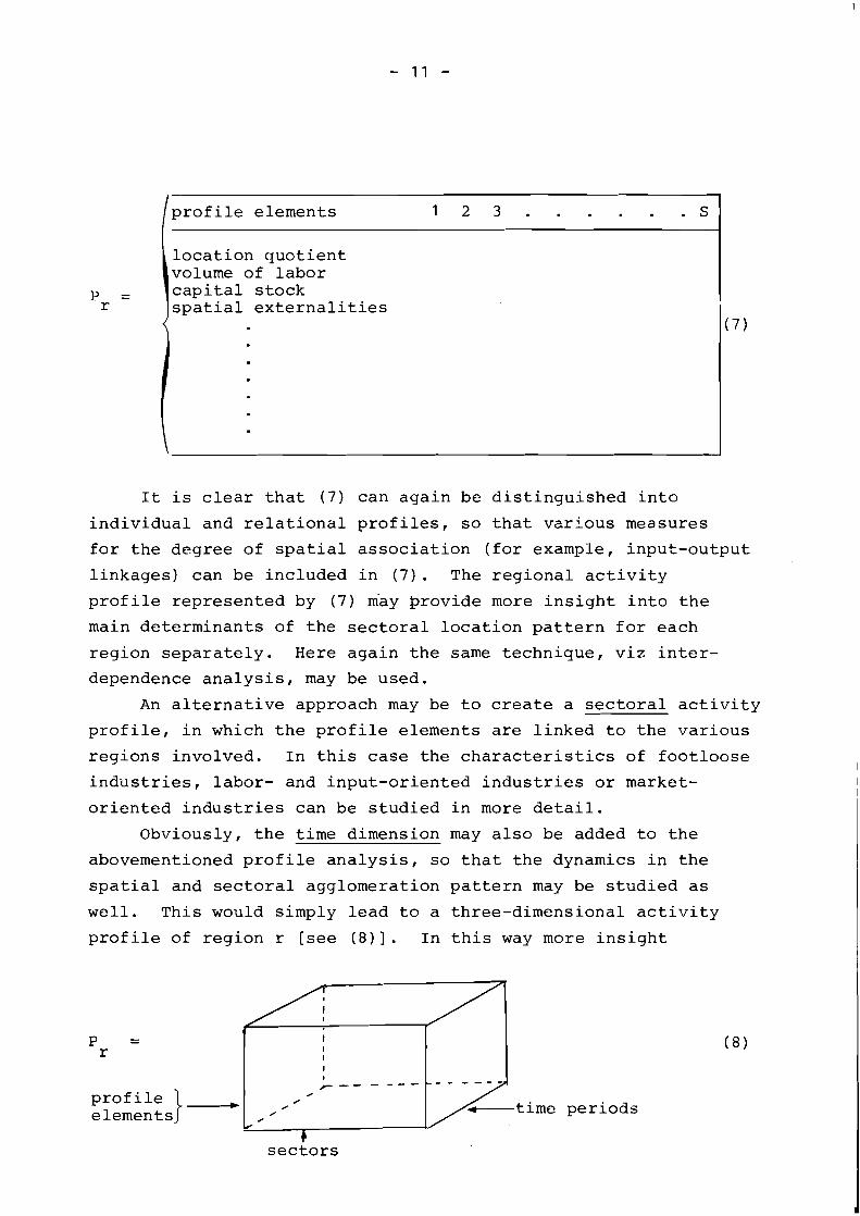
Obviously, the time dimension may also be added to the

abovementioned profile analysis, so that the dynamics in the

spatial and sectoral agglomeration pattern may be studied as

well. This would simply lead to a three-dimensional activity

profile of region r [see (B)]. In this way more insight

P = I

r I I

I I /- - - - - - -

0

0 /

elements 0 time periods

C sectors

may be o b t a i n e d i n t o s h i f t s i n t h e main p r o f i l e e l e m e n t s

d e t e r m i n i n g t h e dynamics o r s p a t i a l a c t i v i t y and agglomerat ion

p a t t e r n s over a number of y e a r s . In te rdependence a n a l y s i s may

a l s o be a u s e f u l t o o l f o r s t u d y i n g t h e s e developments .

Consequent ly , t h e a n a l y s i s may be c a r r i e d o u t i n v a r i o u s

d i r e c t i o n s th rough t h e d a t a m a t e r i a l , l e a d i n g t o r e g i o n - s p e c i f i c ,

s e c t o r - s p e c i f i c o r t i m e - s p e c i f i c r e s u l t s .

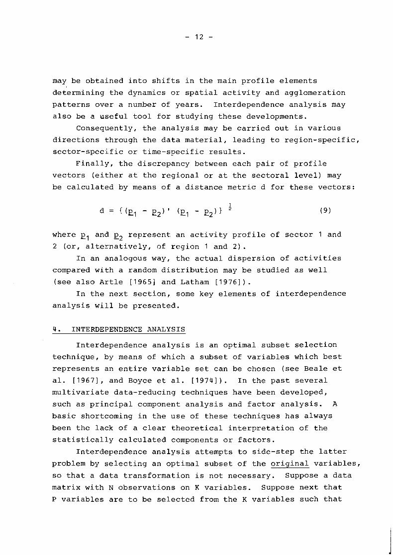
F i n a l l y , t h e d i s c r e p a n c y between each p a i r of p r o f i l e

v e c t o r s ( e i t h e r a t t h e r e g i o n a l o r a t t h e s e c t o r a l l e v e l ) may

be c a l c u l a t e d by means o f a d i s t a n c e m e t r i c d f o r t h e s e v e c t o r s :

where p1 and p2 r e p r e s e n t an a c t i v i t y p r o f i l e o f s e c t o r 1 and

2 ( o r , a l t e r n a t i v e l y , of r e g i o n 1 and 2 ) . I n an analogous way, t h e a c t u a l d i s p e r s i o n o f a c t i v i t i e s

compared w i t h a random d i s t r i b u t i o n may be s t u d i e d a s w e l l

(see a l s o A r t l e [I9651 and Latham [I9761 ) . I n t h e n e x t s e c t i o n , some key e l e m e n t s o f in te rdependence

a n a l y s i s w i l l be p r e s e n t e d .

4 . INTERDEPENDENCE ANALYSIS

In te rdependence a n a l y s i s i s an o p t i m a l s u b s e t s e l e c t i o n

t e c h n i q u e , by means of which a s u b s e t of v a r i a b l e s which b e s t

r e p r e s e n t s an e n t i r e v a r i a b l e se t can be chosen (see Bea le e t

a l . [ 1 9 6 7 ] , and Boyce e t a l . [ 1 9 7 4 ] ) . I n t h e p a s t s e v e r a l

m u l t i v a r i a t e d a t a - r e d u c i n g t e c h n i q u e s have been deve loped ,

such a s p r i n c i p a l component a n a l y s i s and f a c t o r a n a l y s i s . A

b a s i c shor tcoming i n t h e u s e of t h e s e t e c h n i q u e s h a s a lways

been t h e l a c k of a c l e a r t h e o r e t i c a l i n t e r p r e t a t i o n o f t h e

s t a t i s t i c a l l y c a l c u l a t e d components o r f a c t o r s .

In te rdependence a n a l y s i s a t t e m p t s t o s i d e - s t e p t h e l a t t e r

problem by s e l e c t i n g a n o p t i m a l s u b s e t o f t h e o r i g i n a l v a r i a b l e s ,

s o t h a t a d a t a t r a n s f o r m a t i o n i s n o t n e c e s s a r y . Suppose a d a t a

m a t r i x w i t h N o b s e r v a t i o n s on K v a r i a b l e s . Suppose n e x t t h a t

P v a r i a b l e s a r e t o be s e l e c t e d from t h e K v a r i a b l e s such t h a t

these F variables reflect an optimal correspondence with respect

to the original data set. Consequently, (K - P) variables are to be 'rejected' or eliminated.

Now the interdependence analysis starts with a successive

regression analysis between the 'dependent' (K - P) variables to be rejected and the 'independent' P -variables to be retained.

Suppose that 1 X~

is the N x P reduced matrix pertaining to

variables 1, ..., P. Then the following regression equation

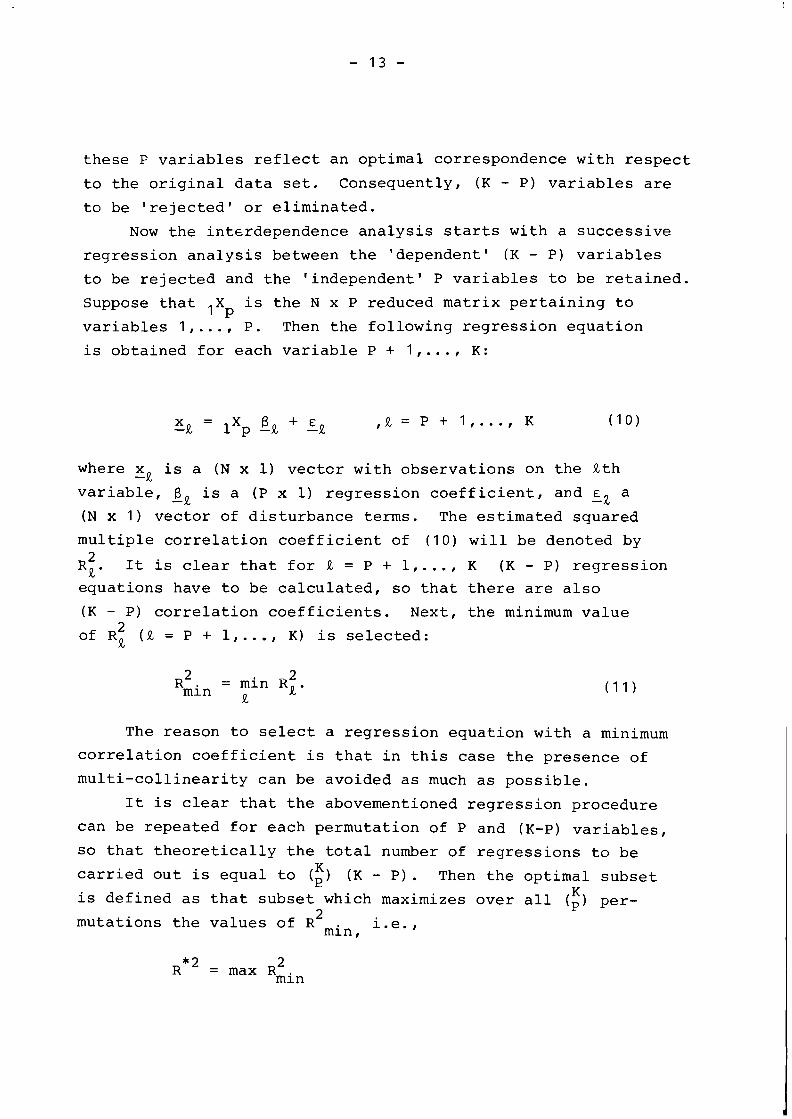
is obtained for each variable P + 1, ..., K:

where x is a (N x 1) vectcr with observations on the Rth -R variable, - BR is a (P x 1) regression coefficient, and E~ a (N x 1) vector of disturbance terms. The estimated squared

multiple correlation coefficient of (10) will be denoted by

R:. It is clear that for R = P + 1,. . . , K (K - P) regression equations have to be calculated, so that there are also

(K - P) correlation coefficients. Next, the minimum value 2

of RR (R = P + 1, ..., K) is selected:

2 2 = min Kg. Rmin

The reason to select a regression equation with a minimum

correlation coefficient is that in this case the presence of

multi-collinearity can be avoided as much as possible.

It is clear that the abovementioned regression procedure

can be repeated for each permutation of P and (K-P) variables,

so that theoretically the total number of regressions to be K carried out is equal to ( p ) (K - P). Then the optimal subset

K is defined as that subset which maximizes over all ( p ) per- 2

mutations the values of R i.e.,

2 R * ~ = max R~~~

Essentially this solution can be seen as the equilibrium

solution of a game procedure, in which the information con-

tained in a data matrix is reduced such that the selected

variables constitute a maximum representation of the information

pattern with a minimum of multicollinearity. This max-min

solution might lead to an enormous computational load, but the

strength of interdependence analysis is that it finds the

optimal subset without a complete enumeration of all possible

regressions. Instead, a set of demarcation criteria and bounding

rules are introduced to speed up the search for an optimal

subset. By means of elimination procedures via critical thres-

hold levels based on statistical properties of the successive

correlation coefficients, the computational work can be

facilitated significantly, so that in principle an optimal

subset can be selected within a reasonable tine limit

(Boyce et al. [I 974 I ) . The appealing feature of interdependence analysis is that

it selects a subset of rather independent variables which have

a maximum correspondence with the original data set without

using arbitrary or artificial data transformations. Hence, the

interpretation of the results is straightforward.

Interdependence analysis has been applied inter alia in

optimal network algorithms (see Boyce et al. [1974]), in multi-

criteria analyses (Ni jkamp [I 977a1) and in multi-dimensional

analyses of human settlements (Nijkamp [1977b]). The experiences

with interdependence analysis are rather favourable so farj

a broader application of this technique may be worthwile.

In the following Section an empirical application of

spatial complex analysis and interdependence analysis will be

presented.

5. EMPIRICAL APPLICATION*

The abovementioned analysis has been applied in an investi-

gation into agglomeration phenomena in the province North-

Holland in the Netherlands. This province has been subdivided

in-to 1 1 separate areas. These areas are mainly based on an

existing spatial delineation of the province concerned for

labor market regions (see Figure 1). For each of these small-

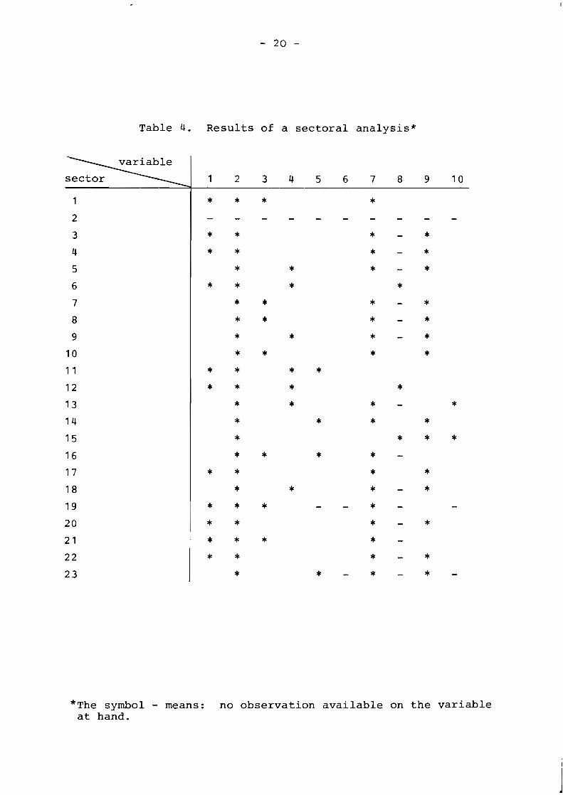
scale regions 23 economic sectors have been distinguished (see

Table 1). Furthermore, in relation to these 1 1 regions and 23

sectors several agglomeration variables and indicators (10 in

total) were employed (see Table 2) . Needless to say, the

data collection at such a detailed spatial level was fraught

with difficulties and often liable to inaccuracies. A total

description of the data base will not be given here but can

be found in Van den Bor [1977]. Suffice it for the moment to

pay somewhat more attention to the definition of the 10 agglomer-

ation variables and indicators included in the spatial complex

analysis. These variables and indicators are:

Table 1. List of economic sectors

1. agriculture & fishery 13. public utilities

2. resource extraction 14. building sector

3. food 15. retailing

4. textile 16. hotels and restaurants

5. leather, rubber & chemicals 17. reparation services

6. wood 18. railway, road and water- way services 7. paper

8. graphical industry

9. building materials

10. metals industry

19. sea & air services

20. communication services

2 1 . banks

11. electro-technical industry 22. insurances

12. transport means 23. real estate

* The author wishes to thank Johan van den Bor who carried out the computational work in this section.

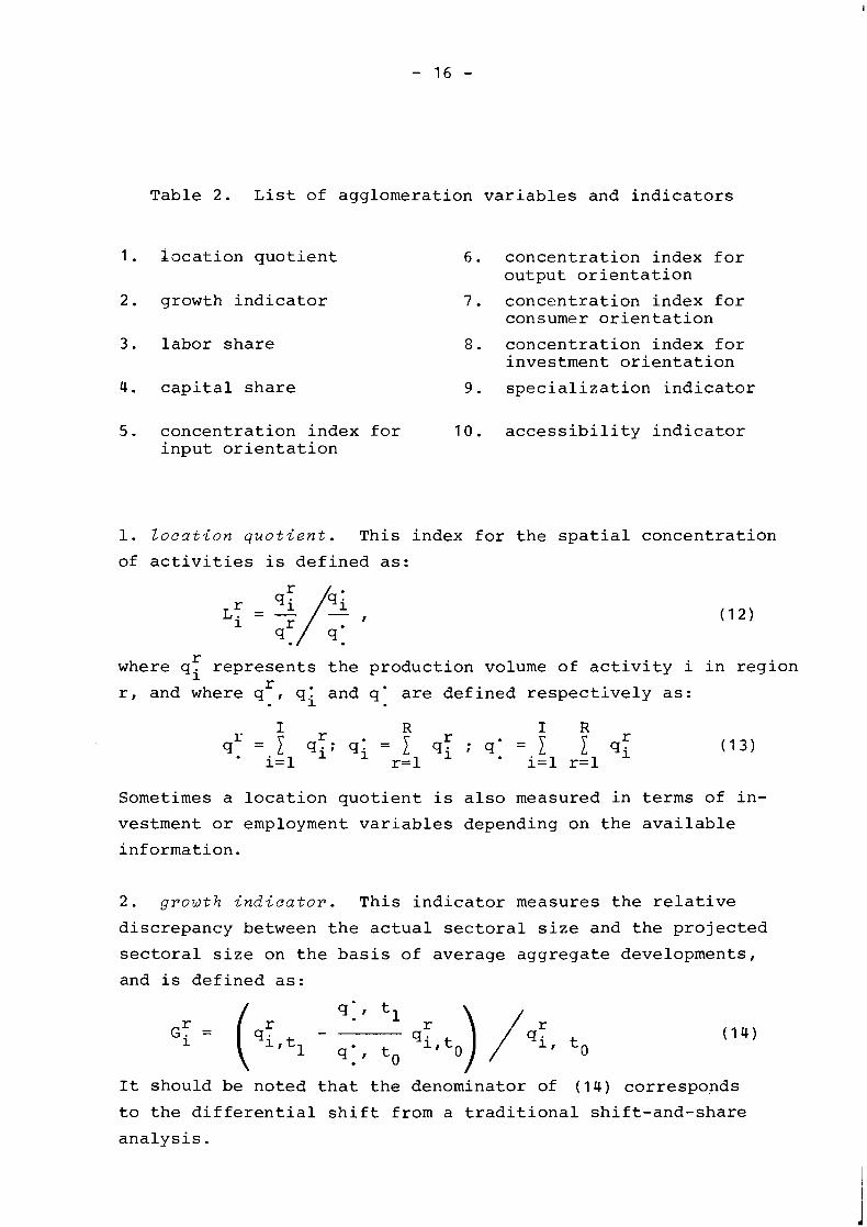
Table 2. List of agglomeration variables and indicators

1. location quotient

2. growth indicator

3. labor share

6. concentration index for output orientation

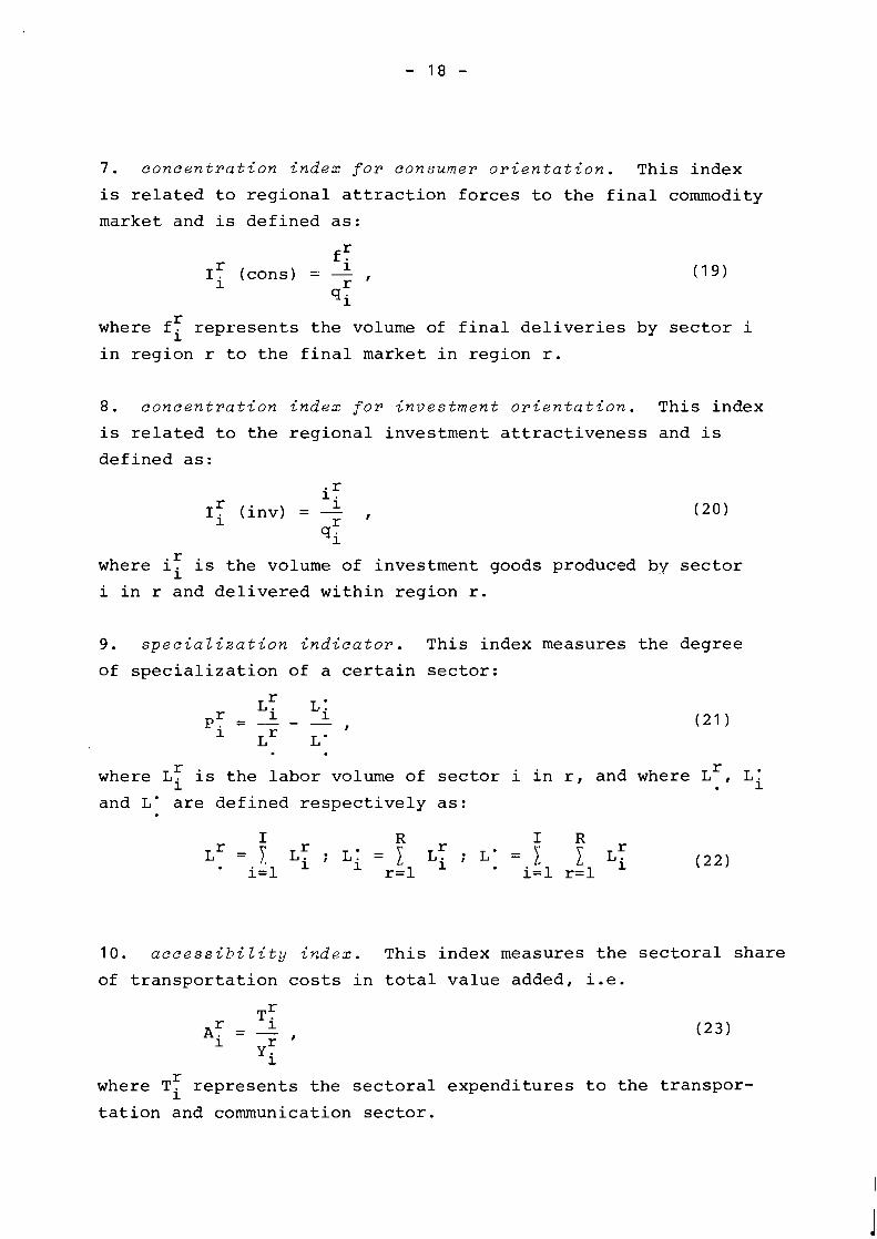
7. concentration index for consumer orientation

8. concentration index for investment orientation

4. capital share 9. specialization indicator

5. concentration index for 10. accessibility indicator input orientation

1. Z o c a t i o n q u o t i e n t . This index for the spatial concentration

of activities is defined as:

r where qi represents the production volume of activity i in region --

r, and where qr, qi and q' are defined respectively as:

Sometimes a location quotient is also measured in terms of in-

vestment or employment variables depending on the available

information.

2 . growth i n d i c a t o r . This indicator measures the relative

discrepancy between the actual sectoral size and the projected

sectoral size on the basis of average aggregate developments,

and is defined as:

It should be noted that the denominator of (14) corresponds

to the differential shift from a traditional shift-and-share

analysis.

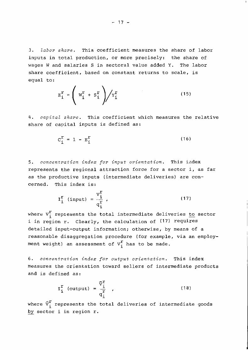
3. Zabor s h a r e . This coefficient measures the share of labor

inputs in total production, or more precisely: the share of

wages W and salaries S in sectoral value added Y. The labor

share coefficient, based on constant returns to scale, is

equal to:

4 . c a p i t a l s h a r e . This coefficient which measures the relative

share of capital inpts is defined as:

5 . c o n c e n t r a t i o n i n d e x f o r i n p u t o r i e n t a t i o n . This ii~dex

represents the regional attraction force for a sector if as far

as the productive inputs (intermediate deliveries) are con-

cerned. This index is:

r V; Ii (input) = - r 9;

where V; represents the total intermediate deliveries - to sector

i in region r. Clearly, the calculation of (17) requires

detailed input-output information; otherwise, by means of a

reasonable disaggregation procedure (for example, via an employ-

ment weight) an assessment of V: has to be made.

6 . c o n c e n t r a t i o n i n d e x f o r o u t p u t o r i e n t a t i o n . This index

measures the orientation toward sellers of intermediate products

and is defined as:

r Tt Ii (output) = - , r (78)

qi

where 55 represents the total deliveries of intermediate goods b~ sector i in region r.