Embed Size (px)
Citation preview

A spacetime derivation of the Lorentzian
OPE inversion formula
David Simmons-Duffin,a,b Douglas Stanford,b and Edward Wittenb
aWalter Burke Institute for Theoretical Physics, Caltech, Pasadena, CA 91125bInstitute for Advanced Study, Princeton, NJ 08540
Abstract
Caron-Huot has recently given an interesting formula that determines OPE data
in a conformal field theory in terms of a weighted integral of the four-point func-
tion over a Lorentzian region of cross-ratio space. We give a new derivation of
this formula based on Wick rotation in spacetime rather than cross-ratio space.
The derivation is simple in two dimensions but more involved in higher dimen-
sions. We also derive a Lorentzian inversion formula in one dimension that sheds
light on previous observations about the chaos regime in the SYK model.
arX
iv:1
711.
0381
6v1
[he
p-th
] 1
0 N
ov 2
017

Contents
1 Introduction 2
2 Two dimensions 5
2.1 Wick rotation and the double commutator . . . . . . . . . . . . . . . . . . . 7
2.2 Rewriting in terms of cross-ratios . . . . . . . . . . . . . . . . . . . . . . . . 9
3 Higher dimensions 10
3.1 Initial setup and gauge fixing . . . . . . . . . . . . . . . . . . . . . . . . . . 11
3.2 Isolating a null direction . . . . . . . . . . . . . . . . . . . . . . . . . . . . . 12
3.3 A shortcut (optional) . . . . . . . . . . . . . . . . . . . . . . . . . . . . . . . 13
3.4 Wick rotation and the double commutator . . . . . . . . . . . . . . . . . . . 14
3.5 Averaging over null directions . . . . . . . . . . . . . . . . . . . . . . . . . . 15
3.6 Changing gauge . . . . . . . . . . . . . . . . . . . . . . . . . . . . . . . . . . 16
3.7 Evaluating the integral for small cross ratios . . . . . . . . . . . . . . . . . . 17
3.8 Writing in terms of cross ratios . . . . . . . . . . . . . . . . . . . . . . . . . 20
4 One dimension 22
5 Discussion 25
A Details on the partial waves 26
A.1 Relation to conformal blocks . . . . . . . . . . . . . . . . . . . . . . . . . . . 26
A.2 Normalization . . . . . . . . . . . . . . . . . . . . . . . . . . . . . . . . . . . 28
A.3 Completeness . . . . . . . . . . . . . . . . . . . . . . . . . . . . . . . . . . . 29
B Subtleties in the Euclidean formula 33
B.1 Spurious poles in the continuation off the principal series . . . . . . . . . . . 33
B.2 Non-normalizable contributions to the four-point function . . . . . . . . . . . 34
C A different way of obtaining BJ(η) 36
D Subtleties in the Lorentzian formula 38
D.1 No extra singularities during the v contour deformation . . . . . . . . . . . . 38
D.2 The requirement that J > 1 . . . . . . . . . . . . . . . . . . . . . . . . . . . 39
1

1 Introduction
The operator product expansion in a conformal field theory implies that one can write a
four-point correlation function as a discrete sum of conformal blocks corresponding to the
physical operators of the theory:
〈O1(x1) · · ·O4(x4)〉 =∑∆,J
p∆,JG∆i∆,J(xi). (1.1)
The conformal block G∆i∆,J(xi) gives the total contribution to their four-point function coming
from operators in a multiplet with a primary of dimension ∆ and spin J . The superscript ∆i
represents dependence on the dimensions of the four external operators Oi. The coefficient
p∆,J is a product of OPE coefficients, and the sum runs over the particular set of operators
that we have in a given theory.
It is sometimes useful to think about this expansion as arising from a more primitive
formula where we simply expand the four-point function in terms of a complete basis of
single-valued functions Ψ∆i∆,J(xi).
1 These functions are sometimes called conformal partial
waves, and they are given by conformal blocks plus “shadow” blocks with ∆→ ∆ ≡ d−∆,
Ψ∆i∆,J(xi) = K∆3,∆4
∆,JG∆i
∆,J(xi) +K∆1,∆2
∆,J G∆i
∆,J(xi). (1.2)
The K coefficients will be given in (A.6) below. A mathematically complete set of such
functions (in d > 1) consists of partial waves with integer spin and unphysical complex
dimensions, ∆ = d2
+ ir, where r is a nonnegative real number. These are often referred to
as the principal series representations.
In addition to being complete, the principal series wave functions are also orthogonal
in an appropriate sense. There is a conformally-invariant pairing between Ψ∆i∆,J and Ψ∆i
∆′,J ′
where we simply multiply the functions and integrate over all four external points. We also
must divide by the volume of the conformal group SO(d + 1, 1), since the resulting integral
is invariant under simultaneous conformal transformations of the four points. (In practice,
this means we must gauge fix and insert the appropriate Faddeev-Popov determinant.) With
respect to this pairing, we have the orthogonality relation,(Ψ∆i
∆,J ,Ψ∆i
∆′,J ′
)≡∫
ddx1 · · · ddx4
vol(SO(d+1, 1))Ψ∆i
∆,J(xi)Ψ∆i
∆′,J ′(xi) = n∆,J 2πδ(r − r′)δJ,J ′ , (1.3)
where the normalization coefficient n∆,J will be given in (A.15) below. Here ∆ = d2
+ ir and
∆′ = d2− ir′ and we assume r, r′ ≥ 0.
1Such expansions can be thought of in terms of harmonic analysis on the conformal group SO(d+ 1, 1).
Harmonic analysis was first applied to conformal field theory in the 70’s [1–4]. Recently there has been
renewed interest in these methods [5–7], partly due to their role in the large-N solution of the SYK model [8].
2

Using this set of principal series wave functions, the four point function can be written
〈O1(x1) · · ·O4(x4)〉 =∞∑J=0
∫ d2
+i∞
d2
d∆
2πi
I∆,J
n∆,J
Ψ∆i∆,J(xi) + (non-norm.) (1.4)
=∞∑J=0
∫ d2
+i∞
d2−i∞
d∆
2πi
I∆,J
n∆,J
K∆3,∆4
∆,JG∆i
∆,J(xi) + (non-norm.). (1.5)
In the first line we introduced the coefficient function I∆,J , dividing by n∆,J for convenience.
This function I∆,J contains all of the theory-specific information in the four point func-
tion, and it will be the focus of this paper. In the second line we inserted (1.2) and then
absorbed the second term by extending the region of integration of the first term. The
non-normalizable contributions will be discussed in appendix B.2.
We can now understand how to recover the OPE presentation in (1.1): we deform the
contour of integration over ∆ to the right, picking up poles along the real ∆ axis at the
locations of physical operators. The residues are proportional to p∆,J .
Often, we imagine using (1.1) and (1.4) to determine the four-point function in a case
where we know the OPE data or expansion coefficient I∆,J . However, for some applications,
it is useful to imagine applying the logic in reverse. Then we assume that the four-point
function (or some contribution to it) is given, and we want to evaluate the corresponding
OPE or coefficient function I∆,J . To do this we take the pairing of Ψ with the four-point
function. Using (1.3) and (1.4), we find an inversion formula2
I∆,J =(〈O1 · · ·O4〉,Ψ∆i
∆,J
)=
∫ddx1 · · · ddx4
vol(SO(d+1, 1))〈O1 · · ·O4〉Ψ∆i
∆,J(xi). (1.6)
In this formula, all four points are integrated over d-dimensional Euclidean space. By par-
tially gauge-fixing the SO(d+1, 1) symmetry, this can be reduced to an integral over cross
ratios.
We would like to emphasize that (1.6) is quite trivial, simply expressing the orthogo-
nality of the partial waves. Recently, a much more interesting formula for I∆,J has been
presented by Caron-Huot [9]. This involves an integral over two Lorentzian regions, with an
integrand given by a special type of conformal block multiplied by a double commutator,
either 〈[O1, O3][O2, O4]〉 or 〈[O1, O4][O2, O3]〉, depending on the region. This formula has
several advantages, such as the fact that it can be analytically continued in the spin J , and
that for real dimension and spin the integrand satisfies positivity conditions.
The purpose of this paper is to give an alternate derivation of Caron-Huot’s more in-
teresting formula. Our strategy is as follows. We start from the formula (1.6), and we
represent the Ψ function using the shadow representation, as an integral over a fifth point.
The formula for I∆,J is now a conformally-invariant integral over five points in Euclidean
2We use the notation that Oi is always at position xi unless otherwise specified.
3

space. The idea is to Wick-rotate and deform the contour of integration over these points.
We end up integrating over a subregion of Lorentzian spacetime such that e.g. x3 is in the
future of x1 and x2 is the future of x4, but all other relationships between points are space-
like. After integrating out some of the coordinates using conformal symmetry, this becomes
Caron-Huot’s formula.
In slightly more detail, the specific Wick rotation is simplest to describe after making a
partial gauge fixing of SO(d+1, 1), where we set x1 = (1, 0, 0, · · · ), x2 = 0, and x5 =∞. We
then Wick-rotate the integral over the remaining points x3, x4. The integrand has branch
point singularities at locations where x3 or x4 become null separated from x1 or x2. We
deform the contour for each of x3, x4 to pick up the discontinuity across the corresponding
branch cuts. For each of x3, x4, the discontinuity leads to a commutator between one of
O3, O4 and O1, O2. Deforming the contour in both variables (which is valid for J > 1) gives
double commutators of the type described above, integrated over a subset of the Lorentzian
space for x3, x4:
I∆,J = −CJ(1)
[∫3>1,2>4
ddx3ddx4
vol(SO(d−1))
〈[O4, O2][O1, O3]〉|x34|J+2d−∆3−∆4−∆
(m · x34)Jθ(m · x34) (1.7)
+ (−1)J∫
4>1,2>3
ddx3ddx4
vol(SO(d−1))
〈[O3, O2][O1, O4]〉|x34|J+2d−∆3−∆4−∆
(−m · x34)Jθ(−m · x34)
].
Here m is the null vector mµ = (1, 1, 0, . . . , 0), the second component is the time direction.
The notation i > j means that xi is in the future lightcone of xj. In the regions where the θ
step functions are nonzero, all pairs of points not indicated in the subscript to the integral
are spacelike separated. The CJ(1) constant is specified in footnote 5. The fact that we have
a natural analytic continuation in spin J (apart from the (−1)J factor) is obvious already
from (1.7).
As a final step, this integral can be simplified to Caron-Huot’s formula (an integral over
cross ratios only) by un-gauge-fixing this integral and re-gauge-fixing in a new gauge that
separates the integration variables into cross ratios and everything else. The integral over
everything else gives a multiple of a funny conformal block with “dimension” given by J+d−1
and “spin” given by ∆− d+ 1. Concretely,
I∆,J = α∆,J
[(−1)J
∫ 1
0
∫ 1
0
dχdχ
(χχ)d|χ− χ|d−2G∆i
J+d−1,∆−d+1(χ, χ)〈[O3, O2][O1, O4]〉
T∆i(1.8)
+
∫ 0
−∞
∫ 0
−∞
dχdχ
(χχ)d|χ− χ|d−2G∆i
J+d−1,∆−d+1(χ, χ)〈[O4, O2][O1, O3]〉
T∆i
].
In this expression, T∆i is a factor of external positions that we strip off to make the four-point
function depend only on the cross ratios, see (3.29). The α coefficient is given in (3.42). This
4

formula is precisely Caron-Huot’s inversion formula once we convert to his c(J,∆) using
c(J,∆) =I∆,J
n∆,J
K∆3,∆4
∆,J. (1.9)
Note that this translation contains a factor of (−1)J .
In the rest of the paper we will spell out the details in this argument. Although each
step is simple, there are several steps involved. In two dimensions some of these can be
combined, and the presentation is significantly simpler. We will go through this case first. We
also present a separate derivation for the interesting case of dimension one, where lightcone
coordinates are not available but Caron-Huot’s formula does have a nontrivial analog, which
played a role in [8].
2 Two dimensions
In this section we will derive the Lorentzian OPE inversion formula for the special case of a
conformal field theory in two spacetime dimensions. We treat this case separately because
some aspects are different (and simpler!) than the d > 2 case, which we will discuss in
the next section. To further simplify the analysis, we will specialize to the case where the
external dimensions are equal ∆1 = ∆2 = ∆3 = ∆4 = ∆O. We will study general ∆i when
we move to higher dimensions.
In two dimensions, the conformal group SL(2,R)×SL(2,R) has two independent quadratic
Casimirs, associated with the two SL(2,R) factors. Eigenfunctions of the Casimirs are la-
beled by a pair of left and right weights (h, h), where the dimension is ∆ = h + h and the
spin is J = |h− h|.3 The eigenfunctions are given by the shadow representation
Ψ∆O
h,h(zi, zi) =
1
|z12|2∆O |z34|2∆OΨh,h(zi, zi)
Ψh,h(zi, zi) =
∫d2z5
(z12
z15z25
)h(z12
z15z25
)h(z34
z35z45
)1−h(z34
z35z45
)1−h
. (2.1)
As usual in the shadow representation, Ψh,h is an eigenvector of the Casimirs because it is a
linear combination of products of three-point functions, each of which is an eigenvector of the
Casimirs. Note that the partial wave for the exchange of a symmetric traceless tensor (STT)
would be Ψh,h + Ψh,h, because STT representations are reducible in 2-dimensions (when the
spin J = |h−h| is nonzero). Thus, Ψh,h is not quite analogous to Ψ∆i∆,J in higher dimensions,
which is associated to STTs. This point will be important later. Our normalization of the
two dimensional shadow integral also differs from what we will define in higher dimensions
by a factor of 2J .
3Note that h is not in general the complex conjugate of h.
5

The expansion of the four-point function in terms of Ψh,h can be written as
〈O1(z1) · · ·O4(z4)〉 =∞∑
`=−∞
∫ ∞0
dr
2π
Ih,hnh,h
Ψ∆O
h,h(zi) + (non-norm.), (2.2)
where h = 1+`+ir2
and h = 1−`+ir2
. The orthogonality relation for these eigenfunctions, in the
sense of (1.3) is [10](Ψ∆O
h,h,Ψ∆O
1−h′,1−h′
)= nh,h 2πδ(r − r′)δ`,`′ , nh,h = − 2π3
(2h− 1)(2h− 1). (2.3)
To extract Ih,h, we must take an inner product between the four-point function 〈O1O2O3O4〉and the partial wave Ψ∆O
1−h,1−h, where ∆O = 2−∆O. On the one hand, this is given by
Ih,h =
∫d2z1 · · · d2z4
vol(SO(3, 1))〈O1O2O3O4〉Ψ∆O
1−h,1−h(zi, zi) (2.4)
=
∫d2χ
|χ|4−2∆O〈O1(0)O2(χ)O3(1)O4(∞)〉Ψ1−h,1−h(0, χ, 1,∞), (2.5)
where in the second line we have chosen the gauge z1 = 0, z2 = χ, z3 = 1, z4 = ∞ (and we
are only writing holomorphic coordinates for brevity). This integral in terms of cross-ratios
χ, χ is the usual Euclidean inversion formula.
On the other hand, plugging in the shadow representation (2.1), we can write the integral
on the RHS of (2.4) as∫d2z1 · · · d2z5
vol(SO(3, 1))
〈O1O2O3O4〉|z12|4−2∆O |z34|4−2∆O
(z12
z15z25
)1−h(z12
z15z25
)1−h(z34
z35z45
)h(z34
z35z45
)h.
(2.6)
As mentioned in the introduction, it is useful to partially gauge fix (2.6) in a different way,
where we choose z1 = 1, z2 = 0, z5 =∞. This gives
Ih,h =
∫d2z3d
2z4
|z34|4−2∆O〈O1O2O3O4〉zh34z
h34. (2.7)
Although (2.7) treats the operators less symmetrically than (2.5), it is natural from a
different point of view. We can think about the four-point function as a kernel that maps
functions of z3, z4 to functions of z1, z2, by integrating over z3, z4. By global conformal invari-
ance, this kernel commutes with the conformal Casimirs, so eigenfunctions of the Casimirs
(like zh34zh34) should also be eigenfunctions of the four-point function. We could have taken
(2.7) as our starting point for the definition of Ih,h. In this case, we could return to the
integral over cross-ratios (2.1) by making the change of variables
χ =z34
(z3 − 1)z4
, (2.8)
6

and integrating over z4.
An important point is that (2.5) and (2.7) only make sense if the spin J is an integer,
because otherwise the functions Ψ1−h,1−h and zh34zh34 would not be single-valued in Euclidean
signature.
2.1 Wick rotation and the double commutator
We will now derive a different formula for Ih,h by doing the integral over z3, z4 in (2.7) in
Lorentzian signature. To Wick rotate, we use the normal Feynman continuation so that we
take τ = (i+ ε)t. Then
|z|2 = x2 + τ 2 = x2 − t2 + iε = uv + iε. (2.9)
Here we have defined u = x − t and v = x + t. With this iε prescription, the integral over
Lorentzian kinematics gives the same answer as the original Euclidean integral. Our integral
becomes
Ih,h = −1
4
∫du3dv3du4dv4
(u34v34)2−∆O〈O1O2O3O4〉uh34v
h34, (2.10)
where the factor of −14
arises because d2z ≡ dτdx = i2dudv.
It will be important to understand the locations of singularities in the complex u, v planes.
In two dimensions, singularities in the four-point function only occur when some pair of
external operators become null separated [11] (in higher dimensions other singularities are
possible, but they will not interfere with the analogous argument). Since we are fixing the
locations of u1, v1 = 1, 1 and u2, v2 = 0, 0, singularities occur when one of the following hold:
u3v3 + iε = 0, u4v4 + iε = 0, (1− u3)(1− v3) + iε = 0, (2.11)
(1− u4)(1− v4) + iε = 0, (u3 − u4)(v3 − v4) + iε = 0. (2.12)
Let us think about fixing u3, u4 and doing the integral over the v3, v4 variables. Suppose
that h = ∆+J2
, h = ∆−J2
with J positive. (If J is negative, we reverse the roles of u, v in the
following.) For sufficiently large J (see appendix D.2), the factor vh34 causes the integrand to
die at large v3, v4. Thus, we can deform the v3, v4 integrals away from the real axis without
worrying about contributions near infinity.
For each of the v variables there are three singularities. If all of the singularities in v3
or v4 are in the upper or lower half planes, then the integral will vanish. This happens if
u31, u32, u34 all have the same sign, or if u41, u42, u43 all have the same sign.
To get a nonvanishing result, we must have one singularity on one side of the axis and two
on the other side, for each of v3 and v4. This requires 0 < u3, u4 < 1. We can then deform
each of the v contours towards the half-plane with only one singularity. This singularity is
7

v3
3~2
3~1 3~4
v4
4~2
4~1
4~3
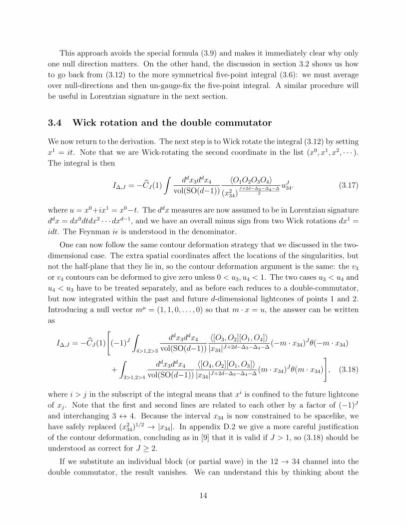
Figure 1: The continuation of v3, v4 in the case where 0 < u3 < u4 < 1. We begin by integrating
both variables over the real axis. We deform the v3 contour in the lower half-plane to pick up
the discontinuity across the branch cut associated with the 3 ∼ 2 singularity, giving the [O3, O2]
commutator. We deform the v4 contour in the upper half-plane and pick up the [O4, O1] singularity.
a branch point, and we can take the branch cut to lie just above or just below the real axis.
The v integrals then take the discontinuities across these branch cuts, which are the same
as the commutators of certain pairs of operators.
For example, when 0 < u3 < u4 < 1 (see figure 1), we deform the v3 contour towards
the lower half-plane around the singularity v32 = −iε/u32 to produce a commutator [O3, O2].
Similarly, we deform the v4 contour towards the upper half-plane around the singularity
v41 = −iε/u41 to produce [O1, O4]. In the other case 0 < u4 < u3 < 1, we obtain the
commutators [O4, O2][O1, O3]. The precise formula we find is
Ih,h = −(−1)J
4
∫R1
du3dv3du4dv4
(u34v34)2−∆O〈[O3, O2][O1, O4]〉uh43v
h43
− 1
4
∫R2
du3dv3du4dv4
(u34v34)2−∆O〈[O4, O2][O1, O3]〉uh34v
h34, (2.13)
where the two integration regions are defined by
R1 : v3 < 0, v4 > 1, 0 < u3 < u4 < 1,
R2 : v3 > 1, v4 < 0, 0 < u4 < u3 < 1. (2.14)
The factor of (−1)J comes from writing zh34zh34 → (−1)Juh43v
h43. One way to summarize the
regions R1, R2 is that the operators in the commutators are timelike separated and all other
pairs are spacelike separated, see figure 2.
Note that after our contour deformation, the integrals above can be analytically continued
in J . For example, the first integral is over a Lorentzian region where u43 and v43 are real
and positive, so there is no issue with single-valuedness. The factor (−1)J means that it is
natural to analytically continue C(h, h) separately for even and odd J .
8

3
21
4
R
2=(0,0)1=(1,1)
1
4
21
3
R2
v
u
Figure 2: We show typical configurations for points 3 and 4 within regions R1 and R2. The
dotted line is not fixed in place, it is only to emphasize that points 3 and 4 must be spacelike
separated. Time goes up.
2.2 Rewriting in terms of cross-ratios
To make contact with Caron-Huot’s formula, we would like to use the fact that the four-point
function (and the commutators) depend only on the cross ratios. Given that u1 = v1 = 1
and u2 = v2 = 0, these reduce to
χ =u34
(u3 − 1)u4
, χ =v34
(v3 − 1)v4
. (2.15)
We can solve these equations for u3, v3 and change variables in the integral, so that we have
an integral over u4, v4, χ, χ. Because the four-point function depends only on χ, χ, we can
then do the integral over u4, v4 explicitly, getting exprssions involving the SL(2,R) conformal
block
k2h(χ) ≡ χh2F1(h, h, 2h, χ), k2h(χ) ≡ (−χ)h2F1(h, h, 2h, χ). (2.16)
The final answer one finds is
Ih,h = −1
4
Γ(h)2
Γ(2h)
Γ(1−h)2
Γ(2−2h)
[(−1)J
∫ 1
0
∫ 1
0
dχdχ
(χχ)2−∆O〈[O3, O2][O1, O4]〉k2h(χ)k2(1−h)(χ)
+
∫ 0
−∞
∫ 0
−∞
dχdχ
(χχ)2−∆O〈[O4, O2][O1, O3]〉k2h(χ)k2(1−h)(χ)
]. (2.17)
One can check that this formula agrees with [9] once we translate using (1.9) which for this
special case reads
c(J,∆) =(−1)J
2π2
Γ(h)2
Γ(2h−1)
Γ(2−2h)
Γ(1−h)2Ih,h. (2.18)
where J = h− h and ∆ = h+ h.
9

3 Higher dimensions
Our discussion in higher dimensions will mirror the one in two dimensions, but with some
new complications. Firstly, note that our two-dimensional derivation required a choice that
depended on the sign of h − h. However, the partial wave for a symmetric traceless tensor
(STT) contains two terms with the role of h and h swapped: Ψh,h+Ψh,h. If we take an inner
product of 〈O1O2O3O4〉 with a STT partial wave, we obtain (2.10) with uh34vh34 replaced by
uh34vh34 + uh34v
h34. These two terms must be treated separately: for the first term, we must
deform the v contour for fixed u, and for the second term we must deform the u contour for
fixed v. In the previous section, we avoided this complication by only discussing the “chiral
half” of a partial wave. However, in higher dimensions, the complication is unavoidable
because operators transform as STTs. Our approach will be to isolate an individual null
direction (similarly to isolating one of the two terms above), and perform the two-dimensional
contour manipulation for that null direction.
The second complication is that in higher-dimensions, after Wick rotation to Lorentzian
signature and performing a contour manipulation to obtain the double-commutator, the
separation of variables into cross-ratios and non-cross-ratios (as in (2.15)) is more difficult.
To do this, we will un-isolate the null directions by integrating over them. The result can
then be re-interpreted as a gauge-fixed five-point integral, this time in Lorentzian signature.
Choosing a different gauge, we obtain an integral over cross ratios that reproduces Caron-
Huot’s formula.
To summarize, the logical outline of our derivation is as follows:
1. Set up the inner product between the four-point function and a partial wave Ψ∆i∆,J as
an integral over five Euclidean points, with x5 being the point we integrate over in the
shadow representation of Ψ.
2. Choose the gauge x1 = (1, 0, . . . , 0), x2 = (0, . . . , 0), x5 =∞.
3. Isolate a single null direction (using a particular representation of Gegenbauer polyno-
mials discussed below), and Wick rotate to Lorentzian signature.
4. Perform the two-dimensional contour deformation from section 2.1 to obtain a double
commutator and an integral over a restricted Lorentzian region.
5. Integrate over null directions.
6. Un-gauge-fix the integral and then re-gauge-fix in a different gauge that separates the
integration variables into cross-ratios plus non-cross-ratio degrees of freedom.
7. Evaluate the integral over non-cross-ratio degrees of freedom in the limit of small cross-
ratios. This fixes the integral for all values of the cross ratios because we know it has
to give an eigenfunction of the conformal Casimir.
10

3.1 Initial setup and gauge fixing
With these preliminaries out of the way, our first task is to write the inner product between
the partial wave and our four-point function as a conformally-invariant integral over five
points. The fifth point arises from the shadow representation of the partial wave, which in
general dimensions has the form:
Ψ∆i∆,J(xi) =
∫ddx5〈O1O2O
µ1···µJ5 〉〈O5,µ1···µJO3O4〉. (3.1)
Here the three-point functions are given by e.g.4
〈O1O2Oµ1···µJ5 〉 =
Zµ1 · · ·ZµJ − traces
|x12|∆1+∆2−∆|x15|∆1+∆−∆2|x25|∆2+∆−∆1, Zµ ≡ |x15||x25|
|x12|
(xµ15
x215
− xµ25
x225
).
(3.2)
This leads to the explicit formula for the partial wave
Ψ∆i∆,J(xi) =
∫ddx5
1
|x12|∆1+∆2−∆|x15|∆1+∆−∆2|x25|∆2+∆−∆1
× 1
|x34|∆3+∆4−∆|x35|∆3+∆−∆4|x45|∆4+∆−∆3
CJ(η), (3.3)
where we have defined the conformal invariant
η =|x15||x25||x12|
|x35||x45||x34|
(~x15
x215
− ~x25
x225
)·(~x35
x235
− ~x45
x245
), (3.4)
and we wrote the sum over polarizations in terms of a Gegenbauer polynomial5 using
|n|J |m|JCJ(n ·m|n||m|
)= (nµ1 · · ·nµJ − traces)(mµ1 · · ·mµJ − traces). (3.5)
Note that CJ(x) is normalized so that the coefficient of xJ is one.
The Euclidean inversion formula (1.6) is an inner product between our four-point function
and the partial wave Ψ∆i
∆,Jwhere we replace all operators by their shadows ∆ = d−∆. Using
the shadow representation of this partial wave, (1.6) becomes
I∆,J =
∫ddx1 · · · ddx5
vol(SO(d+1, 1))〈O1O2O3O4〉〈O1O2O
µ1···µJ5 〉〈O5,µ1···µJ O3O4〉. (3.6)
This is a conformally-invariant integral. As in the two-dimensional case, it will be helpful
to partially fix the gauge for the conformal group by setting x5 =∞, x1 = (1, 0, . . . , 0) and
4When we write a two- or three-point function, we mean a conformally-invariant structure with the given
quantum numbers (with a simple normalization that we specify). In particular, three-point functions don’t
include OPE coefficients. By contrast, the four-point function 〈O1O2O3O4〉 can be thought of as a physical
correlation function in some theory.5We define CJ(x) ≡ Γ(J+1)Γ( d−2
2 )
2JΓ(J+ d−22 )
Cd/2−1J (x) where C
d/2−1J (x) ≡ Γ(J+d−2)
Γ(J+1)Γ(d−2) 2F1(−J, J +d−2, d−12 , 1−x
2 ).
11

x2 = (0, . . . , 0). We can define vol(SO(d+ 1, 1)) so that gauge-fixing three points to 0, 1,∞gives a Faddeev-Popov determinant of 1. The above formula then becomes
I∆,J =
∫ddx3d
dx4
vol(SO(d−1))
〈O1O2O3O4〉|x34|2d−∆3−∆4−∆
CJ
(x34 · x12
|x34||x12|
), (3.7)
where SO(d−1) is the stabilizer group of three fixed points. Our convention for the measure
on SO(n) is that a 2π-rotation should have length 2π. This gives
vol(SO(n)) = vol(Sn−1)vol(SO(n−1)). (3.8)
3.2 Isolating a null direction
We cannot perform our contour manipulation with (3.7) because for large J , the Gegenbauer
polynomial CJ
(x34·x12
|x34||x12|
)grows in every null direction. Instead, we would like to find an
integrand that does not grow along some null direction.
Consider the following representation of the Gegenbauer polynomial:
|x|JCJ(x0
|x|
)=
CJ(1)
vol(Sd−2)
∫Sd−2
dd−2e (n · x)J , (3.9)
where e is a unit vector in d − 1 dimensions, the integral is over the d − 2 sphere, and
n = (1, ie) is a null vector. Because n is null, the right-hand side is a harmonic polynomial
of degree J in x (and thus it transforms as a traceless symmetric tensor of spin J). It is a
function of x0 and |x| alone because it involves an average over transverse rotations. These
conditions uniquely specify the Gegenbauer polynomial up to some constant, which we have
fixed out front.6
Plugging (3.9) into (3.7) gives
I∆,J =CJ(1)
vol(Sd−2)
∫ddx3d
dx4
vol(SO(d−1))
∫Sd−2
de〈O1O2O3O4〉
|x34|J+2d−∆3−∆4−∆(x0
34 + ie · ~x34)J . (3.11)
In this formula, we are averaging over rotations that fix x12. However, the four-point function
is invariant under such rotations, so the answer is given by fixing e to a unit vector of our
6One way to understand why the (d−2)-dimensional integral (3.9) gives a natural object in d-dimensions is
as follows. After Wick rotating x0 → ix0 and redefining n→ −in (note that this is not the Wick rotation we
do in section 3.4), the integral (3.9) becomes a manifestly SO(d− 1, 1)-invariant integral over the projective
null-cone in d-dimensions:
|x|J |y|2−d−J CJ
(x · y|x||y|
)∝ 1
vol(R+)
∫ddn δ(n2)θ(n0)(n · x)J(n · y)2−d−J , (3.10)
where y = (1, 0, . . . , 0). Integrals of exactly the same type in (d+2)-dimensions appeared in [12], where they
are helpful for understanding the shadow representation of conformal blocks.
12

choice and multiplying by vol(Sd−2). For example, let us choose e = (0, 1, 0, . . . , 0), giving
I∆,J = CJ(1)
∫ddx3d
dx4
vol(SO(d−1))
〈O1O2O3O4〉|x34|J+2d−∆3−∆4−∆
(x034 + ix1
34)J . (3.12)
Equation (3.12) is now completely analogous to (2.7) in the 2d case.
3.3 A shortcut (optional)
A simpler way to arrive at (3.12) is to think of the four-point function as a kernel taking
functions of x3,4 to functions of x1,2 by integration over x3,4. As discussed in the 2d case,
this kernel commutes with the conformal Casimirs, and hence they can be simultaneously
diagonalized. Consider the eigenvector 〈O3O4O5〉 where O5 has dimension ∆ and spin J .
Let the eigenvalue of the four-point function be k∆,J ,
k∆,J〈O1O2Oµ1···µJ5 〉 =
∫ddx3d
dx4〈O1O2O3O4〉〈O3O4Oµ1···µJ5 〉. (3.13)
We can relate k∆,J to I∆,J by taking an inner product of both sides with the shadow three-
point function 〈O1O2O5〉,
k∆,J
∫dx1dx2dx5
vol(SO(d+1, 1))〈O1O2O
µ1···µJ5 〉〈O1O2O5,µ1···µJ 〉
=
∫dx1 · · · dx5
vol(SO(d+1, 1))〈O1O2O3O4〉〈O1O2O5,µ1···µJ 〉〈O
µ1···µJ5 O3O4〉
= I∆,J . (3.14)
The constant on the left-hand side can be computed by gauge fixing x1 = 0, x2 = e, x5 =∞for some unit vector e,∫
dx1dx2dx5
vol(SO(d+1, 1))〈O1O2O
µ1···µJ5 〉〈O1O2O5,µ1···µJ 〉
=1
vol(SO(d−1))〈O1(0)O2(e)Oµ1···µJ
5 (∞)〉〈O1(0)O2(e)O5,µ1···µJ (∞)〉
=CJ(1)
vol(SO(d−1)). (3.15)
Thus
k∆,JCJ(1)
vol(SO(d−1))= I∆,J . (3.16)
Now we can set x5 =∞, x1 = (1, 0, . . . , 0) and x2 = (0, . . . , 0) in (3.13) and contract with a
null vector n = (1, i, 0, . . . , 0), to obtain (3.12).
13
This approach avoids the special formula (3.9) and makes it immediately clear why only
one null direction matters. On the other hand, the discussion in section 3.2 shows us how
to go back from (3.12) to the more symmetrical five-point integral (3.6): we must average
over null-directions and then un-gauge-fix the five-point integral. A similar procedure will
be useful in Lorentzian signature in the next section.
3.4 Wick rotation and the double commutator
We now return to the derivation. The next step is to Wick rotate the integral (3.12) by setting
x1 = it. Note that we are Wick-rotating the second coordinate in the list (x0, x1, x2, · · · ).The integral is then
I∆,J = −CJ(1)
∫ddx3d
dx4
vol(SO(d−1))
〈O1O2O3O4〉(x2
34)J+2d−∆3−∆4−∆
2
uJ34. (3.17)
where u = x0+ix1 = x0−t. The ddx measures are now assumed to be in Lorentzian signature
ddx = dx0dtdx2 · · · dxd−1, and we have an overall minus sign from two Wick rotations dx1 =
idt. The Feynman iε is understood in the denominator.
One can now follow the same contour deformation strategy that we discussed in the two-
dimensional case. The extra spatial coordinates affect the locations of the singularities, but
not the half-plane that they lie in, so the contour deformation argument is the same: the v3
or v4 contours can be deformed to give zero unless 0 < u3, u4 < 1. The two cases u3 < u4 and
u4 < u3 have to be treated separately, and as before each reduces to a double-commutator,
but now integrated within the past and future d-dimensional lightcones of points 1 and 2.
Introducing a null vector mµ = (1, 1, 0, . . . , 0) so that m · x = u, the answer can be written
as
I∆,J = −CJ(1)
[(−1)J
∫4>1,2>3
ddx3ddx4
vol(SO(d−1))
〈[O3, O2][O1, O4]〉|x34|J+2d−∆3−∆4−∆
(−m · x34)Jθ(−m · x34)
+
∫3>1,2>4
ddx3ddx4
vol(SO(d−1))
〈[O4, O2][O1, O3]〉|x34|J+2d−∆3−∆4−∆
(m · x34)Jθ(m · x34)
], (3.18)
where i > j in the subscript of the integral means that xi is confined to the future lightcone
of xj. Note that the first and second lines are related to each other by a factor of (−1)J
and interchanging 3 ↔ 4. Because the interval x34 is now constrained to be spacelike, we
have safely replaced (x234)1/2 → |x34|. In appendix D.2 we give a more careful justification
of the contour deformation, concluding as in [9] that it is valid if J > 1, so (3.18) should be
understood as correct for J ≥ 2.
If we substitute an individual block (or partial wave) in the 12 → 34 channel into the
double commutator, the result vanishes. We can understand this by thinking about the
14
shadow representation
Ψ ∼∫ddx5〈O1O2O5〉〈O5O3O4〉, (3.19)
where we Wick rotate x5 to Lorentzian signature. A nonzero commutator [O3, O2] requires
a singularity when O3 and O2 are lightlike separated. Although the integrand has no such
singularities, the integral can have a singularity coming from the regime where x5 is light-
like separated from x2 and x3. However, generically x5 cannot be simultaneously lightlike
separated from O2O3 and O1O4. This is possible for special configurations of O1 · · ·O4, but
the singularities associated with such configurations can be avoided when computing dis-
continuities. Hence, the double commutator [O2, O3][O1, O4] vanishes in (3.19). A nonzero
contribution to (3.18) only comes about because of an infinite sum over blocks, which pro-
duces new singularities.
3.5 Averaging over null directions
From this point forward in the derivation, the goal is to reduce (3.18) to an integral over
cross ratios. A first step is to average over our arbitrary choice of a null vector. We can do
this by applying a transformation g ∈ SO(d−2, 1) to our vector m, where g acts trivially on
m0 and as a Lorentz transformation on the remaining (d−1) components.
Averaging g over SO(d−2, 1) in e.g. the second line in (3.18) becomes7
−CJ(1)
vol(SO(d−2, 1))
∫3>1,2>4
ddx3ddx4
vol(SO(d−1))
〈[O4, O2][O1, O3]〉|x34|J+2d−∆3−∆4−∆
∫SO(d−2,1)
dg(gm · x34)Jθ(gm · x34).
(3.20)
This expression looks ill-defined, since the volume of SO(d− 2, 1) is infinite. However, after
integrating over g, the integrand of the x3, x4 integral is SO(d−2, 1)-invariant, and therefore
divergent in a way that cancels this factor. If we like, dividing by vol(SO(d − 2, 1)) can be
implemented by gauge-fixing the integral over x3, x4.
The integral over g in (3.20) will give some solution to the Gegenbauer differential equa-
tion, but it will no longer be a polynomial. To find out what function we get, we can use
a SO(d−2, 1) transformation to set x34 = x = (x0, x1, 0, . . . , 0) (with x1 < x0 so that x is
spacelike) and evaluate∫SO(d−2,1)
dg(gm · x)Jθ(gm · x) = vol(SO(d−2))vol(Sd−3)
∫ arccoshx0
x1
0
dβ (sinh β)d−3 (x0 − x1 cosh β)J
= vol(SO(d−2))|x|JBJ
(x0
|x|
). (3.21)
7When we write an indefinite orthogonal group SO(p, q), we always mean the connected component of
the identity in that group.
15

The function BJ(y) can be determined exactly8; however the only property that we will need
is that for large y it behaves as
BJ(y) ∼ πd−2
2 Γ(J + 1)
2JΓ(J + d2)y2−d−J |y| � 1. (3.23)
This is easy to see from the integral in (3.21), taking x1 close to x0 so that |x| is small, and
doing the integral for small β.
Using (3.21), our formula (3.18) can therefore be written as
I∆,J = − CJ(1)
vol(Sd−2)
[(−1)J
∫4>1,2>3
ddx3ddx4
vol(SO(d−2, 1))
〈[O3, O2][O1, O4]〉|x34|2d−∆3−∆4−∆
BJ(−η)
+
∫3>1,2>4
ddx3ddx4
vol(SO(d−2, 1))
〈[O4, O2][O1, O3]〉|x34|2d−∆3−∆4−∆
BJ(η)
]. (3.24)
Here η = x12·x34
|x12||x34| . Note that for the configuration in the first line η < 0 and for the
configuration in the second line, η > 0, so in both cases the argument of BJ is positive.
3.6 Changing gauge
At this point, we would like to separate the integration variables x3, x4 into two cross ratios
χ, χ and everything else, and then do the integral over everything else once and for all.
In practice, it is convenient to do this by recognizing (3.24) as a gauge-fixed version of a
conformally-invariant integral over five points, and then fixing the gauge in a different way
where the cross ratios are manifest.
In this section, we will work with the contribution to I∆,J on the first line in (3.24),
adding in the second line at the end. The un-gauge fixed version of this contribution is
I∆,J ⊃ −CJ(1)
vol(Sd−2)(−1)J
∫4>1,2>3
ddx1 · · · ddx5
vol(SO(d, 2))
〈[O3, O2][O1, O4]〉|x12|∆1+∆2−∆|x15|∆1+∆−∆2|x25|∆2+∆−∆1
× BJ(−η)
|x34|∆3+∆4−∆|x35|∆3+∆−∆4|x45|∆4+∆−∆3
. (3.25)
Here the integral is over configurations such that, apart from the two timelike relations
described in the subscript of the integral, all pairs of points are spacelike separated. In this
expression, η is defined as in (3.4), with a dot product taken in Lorentzian signature.
8After changing variables to z = coshβ, the integral becomes a standard hypergeometric integral. A form
that makes the large y behavior and the branch cut between −1 and 1 obvious can be given after making a
couple of quadratic transformations of the resulting hypergeometric function:
BJ(y) ≡ πd−22 Γ(J+1)
2JΓ(J+d2 )
(1 + y)2−d−J2F1
(J +
d−1
2, J + d− 2, 2J + d− 1,
2
1 + y
). (3.22)
Also, note that in d = 3 dimensions, BJ(y) is a Legendre Q-function.
16

The variables x1 · · ·x5 should be understood as coordinates on the conformal completion
of Minkowski space, i.e. the Lorentzian cylinder Sd−1×R. If we partially gauge-fix by fixing
the location of x5, then the condition that all other points should be spacelike separated
from x5 forces x1 · · ·x4 to be in a single Minkowski diamond of the cylinder. In the natural
Minkowski space coordinates on this patch, x5 is at ∞. If, in these coordinates, we further
gauge-fix so that x1 = (1, 0, . . . , 0) and x2 = 0, then we recover the second line of (3.24).
Instead of picking the gauge that takes us back to (3.24), we will pick a different gauge
where we fix x1 · · ·x4 to locations determined by the cross ratios, and then integrate over
the location of the fifth point, subject to the constraint that it should be spacelike separated
from the others. More precisely, we choose the points x1 · · ·x4 to be located in a 2d plane
and located as in figure 3. The standard conformal cross ratios for this configuration are
χ =4ρ
(1 + ρ)2, χ =
4ρ
(1 + ρ)2. (3.26)
The advantage of this gauge choice is that we have now cleanly separated the cross ratio
degrees of freedom from the other integration variables. The non-cross ratio variables are
simply the location of x5.
4
1
2
3
Figure 3: The configuration of points that we choose, with (u, v) coordinates indicated. The grey
region is spacelike separated from the four points. The 2d slice shown is the plane where the four
points are located. As we move the slice outwards in the transverse directions away from this plane,
the inner and outer grey regions grow and eventually merge, see figure 4.
3.7 Evaluating the integral for small cross ratios
We would like to do the integral over x5:
H∆,J(xi) ≡∫
spacelike
ddx51
|x12|∆1+∆2−∆|x15|∆1+∆−∆2|x25|∆2+∆−∆1
× BJ(−η)
|x34|∆3+∆4−∆|x35|∆3+∆−∆4|x45|∆4+∆−∆3
. (3.27)
17

Here, we assume that x1, . . . , x4 are configured as in figure 3, and x5 ranges over all points
on the cylinder that are spacelike separated from these four points.
By the usual logic of shadow integrals (together with the fact that being spacelike sepa-
rated from all four other points is a conformally covariant notion), this integral is conformally
covariant with weights ∆1, . . . , ∆4 for the four external points. Let us strip off some factors
with the same external weights to obtain a function of conformal cross ratios χ, χ alone:
H∆,J(xi) = T ∆i(xi)H∆,J(χ, χ) =1
|x12|2d|x34|2d1
T∆i(xi)H∆,J(χ, χ), (3.28)
where we distinguish H∆,J(xi) and H∆,J(χ, χ) by their arguments, and
T∆i(xi) ≡1
|x12|∆1+∆2 |x34|∆3+∆4
(|x14||x24|
)∆2−∆1(|x14||x13|
)∆3−∆4
. (3.29)
Note that we take the absolute value of all the intervals |xij| = |(x2ij)|1/2, even though x14 is
timelike. This is because H∆,J(xi) is manifestly real when ∆i,∆, J are real, and we would
like H∆,J(χ, χ) to inherit this property.
The integrand in (3.27) is an eigenfunction of the two-particle quadratic and quartic
conformal Casimirs (with eigenvalues determined by ∆, J) acting on either 1 + 2 or 3 + 4.
Thus, H∆,J(χ, χ) will have the same property. Solutions to these Casimir equations are
determined by their behavior for small values of the cross ratios. So we can pin down
H∆,J(χ, χ) exactly by evaluating it for small χ, χ. In our ρ, ρ coordinates, we can reach this
regime by taking ρ� 1 and ρ� 1, so that9
χ ≈ 4ρ, χ ≈ 4
ρ. (3.30)
For these small values of the cross ratios, it turns out to be straightforward to evaluate the
x5 integral. The integral is dominated by a region where the transverse separation of x5 from
the plane of the other four points is small enough that the lightcones of the four external
operators can be approximated as simpler shapes. This region is illustrated in figure 4.
We will describe x5 by coordinates u, v in the plane of the other four points, and a radius
r in the transverse directions. To organize the integral for small values of the cross ratios, it
is helpful to introduce a small parameter ε� 1, where we take ρ ∼ ε and ρ ∼ ε−1 with some
fixed product ρρ. The important region of the integral comes from u, v of order one and r
of order 1/√ε. As we will see, in this region one can show that −η is large, of order 1/ε. To
summarize, we have
ρ,1
ρ,−η, r2 ∼ 1
ε, u, v ∼ 1. (3.31)
9Note that this corresponds to starting with the standard Euclidean configuration described in [13, 14]
with ρ = ρ, and then applying a large Lorentzian relative boost between the points 1, 2 and 3, 4. This
highly boosted configuration of cross-ratios played an important role in the recent causality-based proof of
the ANEC [15].
18

Figure 4: The region of integration for x5 is the exterior of the lightcones of the four operators.
In the limit of small cross-ratios, the integral is dominated by the region inside the black-outlined
box. The width of the box in the transverse directions is large enough to detect the curvature of
the lightcones, but small enough not to detect their full geometry.
These scalings allow us to simplify the integral considerably. Since −η is large, we can
approximate BJ(−η) using (3.23). Also, for small ε, the quantity η < 0 is determined by a
simplified formula that follows from expanding (3.4):
4η2 ≈ ρ
ρ
(1ρ
+ r2)2
(1−vρ
+ r2)(1+vρ
+ r2)
(ρ+ r2)2
(ρ(1− u) + r2)(ρ(1 + u) + r2). (3.32)
The rest of the integrand can also be simplified, by keeping only the terms of order 1/√ε in the
distances |xij|. For example, |x15| ≈ (ρ(1 + u) + r2)1/2. After making these approximations,
the u and v dependence of the integrand factorizes, as does the region of integration. For
example, the v integral is of the form∫ 1+ρr2
−1−ρr2
dv(1− v + ρr2)a(1 + v + ρr2)b = (2 + 2ρr2)1+a+bΓ(1 + a)Γ(1 + b)
Γ(2 + a+ b). (3.33)
Note that in general, the region of integration is not factorized in u and v, since the bound-
aries of the light cones at finite transverse separation are curved in the u, v plane. However,
the transverse separations r ∼ 1/√ε are small enough that the edges of the “inner” region
remain straight in the u, v plane, although with a separation that depends on r.
After doing the u, v integrals, the final integral over r can be done by changing variables
to y = ρr2 and using
(ρρ)∆−1
2
∫ ∞0
dyyd−4
2 (ρρ+ y)1−∆(1 + y)1−∆ =Γ(d
2−1)2
Γ(d−2)2F1
(∆−1,∆−1,
d−1
2,1−x
2
),
(3.34)
19

where x = 12(√ρρ+ 1√
ρρ) and as always ∆ = d−∆.
Collecting factors of ρ and ρ and translating to cross ratios, one finds that for χ, χ� 1,
H∆,J(χ, χ) ≈ (const.) (χχ)J+d−1
22F1
(∆−1,∆−1,
d−1
2,1−x
2
), (3.35)
where x = 12(√χ/χ +
√χ/χ). More precisely, we have this behavior plus multiplicative
corrections that are analytic at χ = χ = 0. This behavior determines our solution to the
Casimir equations. It takes the form similar to that of a standard conformal block, but with
“dimension” equal to J + d− 1 and “spin” equal to 1− ∆ = ∆− d+ 1.
It is useful to report the constant of proportionality by giving the behavior for χ� χ� 1,
where the hypergeometric function simplifies. We find
H∆,J(χ, χ) ≈ a∆,J (χχ)J+d−1
2
(χ
χ
)−∆−d+12
(3.36)
a∆,J ≡1
2(2π)d−2 Γ(J + 1)
Γ(J + d2)
Γ(∆− d2)
Γ(∆− 1)
Γ(∆12+J+∆2
)Γ(∆21+J+∆2
)Γ(∆34+J+∆2
)Γ(∆43+J+∆2
)
Γ(J + ∆)Γ(J + d−∆),
where ∆ij ≡ ∆i −∆j. Comparing to (A.11), this determines
H∆,J(χ, χ) = a∆,JG∆iJ+d−1,∆−d+1(χ, χ). (3.37)
3.8 Writing in terms of cross ratios
As a final step, we can now write the formula for I∆,J as an integral over cross ratios only.
The result of the last section is that
I∆,J ⊃ −CJ(1)
vol(Sd−2)(−1)J
∫4>1,2>3
ddx1 · · · ddx4
vol(SO(d, 2))〈[O3, O2][O1, O4]〉H∆,J(xi) (3.38)
= − CJ(1)
vol(Sd−2)(−1)J
∫4>1,2>3
ddx1 · · · ddx4
vol(SO(d, 2))
1
|x12|2d|x34|2d〈[O3, O2][O1, O4]〉
T∆i(xi)H∆,J(χ, χ),
where H∆,J is the particular solution to the conformal Casimir equation (3.37).
Let us now gauge fix this integral in the configuration of figure 3. Parameterizing every-
thing in terms of χ = 4ρ(1+ρ)2 and χ = 4ρ
(1+ρ)2 , the gauge-fixed measure becomes∫ddxi
vol(SO(d, 2))
1
|x12|2d|x34|2d→ 1
2vol(SO(d−2))
∫ 1
0
∫ 1
0
1
2
dχdχ
(χχ)d
∣∣∣∣χ− χ2
∣∣∣∣d−2
. (3.39)
Let us make some comments about this result. The quantities inside the integral come from
a Faddeev-Popov determinant.10 The factor vol(SO(d−2)) is the volume of the group of
10To be consistent with our convention that gauge-fixing three points to 0, 1,∞ should give determinant
1, we must additionally divide by the determinant associated with that gauge fixing.
20

transverse rotations. The extra factor of 12
is because of an additional discrete symmetry
that relates two configurations in our integration range. Specifically, there exists an element
of the identity component of SO(d, 2) that exchanges ρ ↔ 1/ρ, or equivalently χ ↔ χ. In
the plane of the four points, we can achieve this with an inversion followed by a dilatation
and boost
(u, v) 7→(ρ
v,
1
ρu
). (3.40)
In two dimensions, an inversion is not continuously connected to the identity. However,
in higher dimensions, we can accompany it with a reflection in a transverse direction to
obtain something continuously connected to the identity. (Different choices of reflection
are related by conjugating by the transverse rotation group SO(d−2).) Hence, to to avoid
double-counting configurations modulo gauge transformations in (3.39), we must divide by
2. We could alternatively restrict the integration region to χ ≤ χ or χ ≤ χ.
We can now write a final expression for I∆,J , as
I∆,J = α∆,J
[(−1)J
∫ 1
0
∫ 1
0
dχdχ
(χχ)d|χ− χ|d−2G∆i
J+d−1,∆−d+1(χ, χ)〈[O3, O2][O1, O4]〉
T∆i(3.41)
+
∫ 0
−∞
∫ 0
−∞
dχdχ
(χχ)d|χ− χ|d−2G∆i
J+d−1,∆−d+1(χ, χ)〈[O4, O2][O1, O3]〉
T∆i
].
In writing this expression we have also added back in the contribution from the second line of
(3.24). The function G∆,J is defined as the conformal block normalized so that for negative
cross ratios satisfying |χ| � |χ| � 1 we have the behavior (−χ)∆−J
2 (−χ)∆+J
2 . Note that this
differs by a phase from the continuation of G∆,J to negative values of χ, χ. The constant out
front is
α∆,J = −a∆,J
2dCJ(1)
vol(SO(d−1)), (3.42)
where a∆,J is defined in (3.36). In order to compare to Caron-Huot, we should use (1.9) to
convert from the inner product I∆,J between the four-point function and a partial wave to
the coefficient c(J,∆) in the partial wave expansion of the four-point function. The equation
for c(J,∆) is then the same as (3.41), but with the constant out front replaced by
α∆,J
n∆,J
K∆3,∆4
∆,J= −(−1)J
Γ(J+∆+∆12
2)Γ(J+∆−∆12
2)Γ(J+∆+∆34
2)Γ(J+∆−∆34
2)
16π2Γ(J + ∆− 1)Γ(J + ∆). (3.43)
We can relate the double commutator to Caron-Huot’s “double discontinuity” dDisc by
defining a stripped four-point function as
〈O1O2O3O4〉 =1
(x212)
∆1+∆22 (x2
34)∆3+∆4
2
(x2
14
x224
)∆2−∆12(x2
14
x213
)∆3−∆42
g(χ, χ). (3.44)
21

Applying the appropriate iε prescriptions in the configuration of figure 3, we find
〈[O3, O2][O1, O4]〉T∆i
= −2 cos(π∆2−∆1+∆3−∆4
2) g(χ, χ) + eiπ
∆2−∆1+∆3−∆4
2 g(χ, χ)
+ e−iπ∆2−∆1+∆3−∆4
2 g�(χ, χ)
≡ −2 dDisc[g(χ, χ)], (3.45)
where g or g� indicates we should take χ around 1 in the direction shown, leaving χ held
fixed. Note that the minus sign in this formula is because our convention for operator
ordering is the one natural for the standard quantization of the theory in a global Minkowski
time, not Rindler time. Similarly,
〈[O4, O2][O1, O3]〉T∆i
= −2 cos(π∆2−∆1+∆4−∆3
2
)g(χ, χ) + eiπ
∆3−∆4+∆2−∆12 g�(χ, χ)
+ e−iπ∆3−∆4+∆2−∆1
2 g(χ, χ), (3.46)
where now g or g� indicates we should take χ around −∞ in the direction shown, leaving
χ held fixed.
Finally, note that the formula in [9] contains the block G∆iJ+d−1,∆−d+1(χ, χ) with un-tilded
external dimensions ∆i, and also some additional factors in the measure. In our formula,
these come from the identity [16]
G∆iJ+d−1,∆−d+1(χ, χ) = ((1− χ)(1− χ))
∆2−∆1+∆3−∆42 G∆i
J+d−1,∆−d+1(χ). (3.47)
With this understanding, and using (3.43), we find that (3.41) agrees precisely with the
formula in [9].11
4 One dimension
There is a one-dimensional analog of Caron-Huot’s formula, although it is less powerful
than in higher dimensions. In one dimension, the complete set of partial waves includes a
discrete series, in addition to the principal continuous series. All wave functions are related
by analytic continuation in ∆, so the same function I∆ describes the inner product of both
principal series and discrete series states with the four-point correlator. This function has
poles for positive Re(∆) that correspond to physical operators of the theory.
The formula we can derive is for a different function I∆ that agrees with I∆ for the discrete
series of integer ∆, but has the additional property that it is analytic (without poles) for
Re(∆) > 1. These properties seems somewhat arbitrary, but there is a good reason for the
existence of such a function. As described in [8], when one continues to the Regge limit in
11We have reversed the subscripts on G∆,J relative to [9].
22

a one dimensional SL(2,R) invariant theory, the discrete states give growing contributions
that naively form a divergent series. If, before continuing to the Regge limit, we write this
sum as an integral over a contour that consists of small circles around the discrete states at
positive integer ∆, and if we use I∆ instead of I∆ in this expression, then we can pull the
contour to the left towards a region with bounded Regge behavior. The absence of poles in
I∆ allows us to do this continuation without picking up growing contributions that would
spoil boundedness in the Regge limit.
In one dimension we do not have light-cone coordinates. However, because the conformal
blocks are simple, it is easy enough to derive the formula directly in cross ratio space.12 In
one dimension the global conformal group is SL(2,R), and a four-point function depends on
a single cross ratio. The wave functions are given by the shadow representation13
Ψ∆O∆,J(τi) =
1
|τ12|2∆O |τ34|2∆OΨ∆,J(χ)
Ψ∆,0(χ) =
∫dτ5
(|τ12||τ15||τ25|
)∆( |τ34||τ35||τ45|
)1−∆
(4.1)
Ψ∆,1(χ) =
∫dτ5
(|τ12||τ15||τ25|
)∆( |τ34||τ35||τ45|
)1−∆
sgn(τ12τ15τ25τ34τ35τ45).
The functions Ψ∆,J on the second two lines depend only on the cross ratio χ = τ12τ34
τ13τ24. The
“spin” J takes two possible values, 0 and 1, and to get a complete basis of functions of χ, we
have to consider both. The functions with J = 0 are symmetric under the transformation
χ→ χ/(χ−1), and the functions with J = 1 are antisymmetric. The reason that we refer to
J as spin is that these expressions are actually the analytic continuation in dimension from
the higher dimensional shadow integrals (3.3). In one dimension η reduces to the product of
sgn factors in Ψ∆,1, so we can understand this factor as C1(η) = η. The fact that we don’t
have other functions is also consistent with the higher dimensional formulas, since when
d = 1 and we consider a value of J ≥ 2, we have CJ(±1) = 0.
The complete set of partial waves corresponds to the principal series ∆ = 12
+ ir in
addition to the even positive integers for Ψ∆,0 and the odd positive integers for Ψ∆,1. We
will be concerned only with the discrete series here. By evaluating the shadow integrals for
12We assume time-reversal symmetry, so that the four-point function is a function of the cross ratio only.
Without time-reversal symmetry, there is an additional discrete invariant. For the shadow representation
without the assumption of time-reversal symmetry, see [17].13As in our d = 2 discussion in section 2, and as in the usual SYK model, we will slightly simplify this
discussion by assuming that the four external operators have the same dimension ∆O.
23

integer ∆, one finds a uniform expression for these discrete states as14
Ψn(χ) = 2Γ(n)2
Γ(2n)k2n(χ), −∞ < χ < 1,
Ψn(χ) =Γ(n)2
Γ(2n)[k2n(χ+ iε) + k2n(χ− iε)] , 1 < χ <∞. (4.2)
In this section we will continue to use the notation for the SL(2,R) block
k2h(χ) ≡ χh2F1(h, h, 2h, χ), k2h(χ) ≡ (−χ)h2F1(h, h, 2h, χ). (4.3)
The notation Ψn is defined for positive integer n = 1, 2, . . . . For even integer n it is equal to
Ψn,0 and for odd integer n it is equal to Ψn,1.
The inner product of these wave functions with the four-point function is defined as
In =
∫ ∞−∞
dχ
χ2g(χ)Ψn(χ), g(χ) ≡ 〈O1O2O3O4〉
〈O1O2〉〈O3O4〉, (4.4)
where g(χ) is the stripped four-point function. It is piecewise analytic, consisting of three
different analytic functions in the regions −∞ < χ < 0, 0 < χ < 1 and 1 < χ < ∞. In the
region 1 < χ <∞, we insert (4.2) and then deform the two terms in opposite half-planes to
the region −∞ < χ < 1. We then find
In =Γ(n)2
Γ(2n)
∫ 1
−∞
dχ
χ2k2n(χ)dDisc[g(χ)]. (4.5)
Here dDisc(χ) is defined as
dDisc[g(χ)] = 2g(χ)− gx(χ)− gx
(χ), (4.6)
where gx and gx
are defined by starting with g(χ) in the region χ > 1 and continuing either
below or above the real axis to the final value of χ < 1.
So far our manipulations are valid for integer n, but we can now continue in n. We have
to take care with defining the continuation of χn for negative χ. To define this we first write
it as (−χ)n(−1)n. Noting that n is even for the discrete states corresponding to J = 0 and
odd for the states corresponding to J = 1, we can write the sign factor as (−1)J . Then
I∆,J =Γ(n)2
Γ(2n)
[(−1)J
∫ 0
−∞
dχ
χ2k2∆(χ)dDisc[g(χ)] +
∫ 1
0
dχ
χ2k2∆(χ)dDisc[g(χ)]
]. (4.7)
14This form of Ψn(χ) for χ < 1 was obtained in [8]. (It arises from eqns. (3.65), (3.66) of that paper
by setting h equal to an integer n.) The result for χ > 1 then follows from the matching conditions
described in [8] between the χ < 1 and χ > 1 wavefunctions. Those wavefunctions behave near χ = 1 as
a + b log |1 − χ|, and the matching conditions say that the coefficients a and b are equal on the two sides.
The following derivation will depend only on the fact that the same function k2n(χ) appears in both lines of
eqns. (4.2), not on any further properties of this function.
24

To summarize, we are making two claims about this function. First, it is analytic in ∆
without poles for real part of ∆ > 1. This is obvious because boundedness in the Regge
limit implies that dDisc[g(χ)] is bounded by a constant for small χ, and then Re(∆) > 1
is enough to ensure that the integral converges. Second, for even integer values of ∆ (for
J = 0) and odd integer values of ∆ (for J = 1), this agrees with I∆,J . This was the content
of the above argument.
5 Discussion
CFT four-point functions are bounded in the Regge limit [18]. Just as in the case of am-
plitudes, nice Regge behavior requires a delicate balance between partial waves. Indeed, an
individual conformal block with spin J grows like e(J−1)t in the Regge limit, where t is a boost
parameter [19]. Thus, if we modified the coefficient of a single block with spin J > 1, we
would completely destroy boundedness in the Regge limit. Caron-Huot’s formula captures
the delicate balance between partial waves by showing that for J > 1 they fit together into
an analytic function of spin with nice properties. This justifies the methods of “conformal
Regge theory” [20, 21]. It also removes the ambiguities associated with asymptotic series
in large-spin perturbation theory [22–30], leading to a finite expansion with no need for re-
summation.15 Positivity of the double-commutator in the Lorentzian inversion formula also
makes it easy to prove bounds on CFT data like Nachtmann’s theorem [22,31,32].
In this work, we have given a new derivation of Caron-Huot’s formula. An advantage of
our approach is that analyticity in spin is almost immediate. After performing the contour
deformation in (3.18), it is clear that I∆,J is an analytic function of spin. In addition, the
derivation in [9] relied on a surprising identity between analytic continuations of conformal
blocks, which we have essentially proved using explicit integral representations for the blocks.
Although we have not focused on this perspective, our inspiration came from thinking
about the Regge limit in the SYK model. There, a special relationship between the standard
kernel (which is essentially k∆,J discussed in section 3.3 for the case of mean field theory) and
a “retarded kernel” (first used in [33]) made it possible to analyze the Regge limit [8,10]. (A
special case of the computation in section 2 of the present paper can be found in Appendix
D of [10].) What we have done in this paper is to show that this relationship holds in general
conformal field theories, not just mean field theory. To make this slightly more explicit, one
views the full four-point function of the CFT as a kernel similar to the ladder kernel in SYK.
The quantity I∆,J is related to the eigenvalues of this kernel, as discussed in section 3.3. The
analog of the retarded kernel from SYK is essentially the double commutator. The fact that
15To compute the large-spin expansion, one applies the Lorentzian inversion formula to the four-point
function in an expansion around the double-lightcone limit χ, 1 − χ � 1. Reaching the double-lightcone
limit from an OPE channel requires summing infinite families of conformal blocks with bounded twist, using
e.g. the techniques of [28,29].
25

the eigenvalues of these kernels are the same is the content of this paper.
We hope that our derivation points the way to generalizations for external operators with
spin and perhaps higher-point functions. A method for deriving Lorentzian inversion formu-
las for correlators with external spins was recently given in [34]. The main idea is to integrate
by parts with conformally-covariant differential operators to reduce the inversion formula to
the scalar case. However, it should be possible to derive a more direct formula, perhaps by
combining our derivation with the methods of [35]. A spinning Lorentzian inversion formula
would be helpful, for example, for studying correlators of stress-tensors.16
The simplest operators to describe in large-spin perturbation theory are “double-twist”
families [22, 23].17 An inversion formula for higher-point functions could make it easier to
study multi-twist operators. It is also interesting to ask whether CFT data can be extended
to analytic functions of other Dynkin indices of SO(d) besides J , which become important
in higher-point functions.
Acknowledgements
We thank Simon Caron-Huot, Abhijit Gadde, Denis Karateev, Petr Kravchuk, Eric Perl-
mutter, and Shu-Heng Shao for discussions. DS is supported by Simons Foundation grant
385600. DSD is supported by Simons Foundation grant 488657. EW is supported in part
by NSF Grant PHY-1606531.
A Details on the partial waves
A.1 Relation to conformal blocks
The partial wave Ψ∆i∆,J(xi) is a sum of two solutions to the conformal Casimir equation with
simple behavior near x12 = 0: a conformal block G∆i∆,J(x) and a shadow block G∆i
∆,J(x) [4,36].
For completeness, we will describe the exact expression and also compute the normalization
factor n∆,J . In the OPE limit x12 → 0, the first term G∆i∆,J(x) behaves how we would expect
from naively taking x12 → 0 in (3.1) inside the integrand. In this limit, G∆i∆,J(x) comes from
the regime of the integral where x5 does not probe the neighborhood near x1,2, so that the
OPE is valid. To compute its coefficient, we can take x12 → 0 in the integrand first and then
perform the resulting integral. (Similarly, to compute the second term, we can take x34 → 0
before integrating.)
16Particularly in holographic theories where the double-commutator kills the contribution of t-channel
double-trace states at orders 1/N0 and 1/N2.17“Double-twist” is equivalent to double-trace in large-N theories.
26

Expanding in small x12, we have
〈O1(x1)O2(x2)Oµ1···µJ (x5)〉 ∼ |x12|∆−∆1−∆2−Jxν112 · · ·x
νJ12〈Oν1···νJ (x1)Oµ1···µJ (x5)〉, (A.1)
where
〈Oν1···νJ (x1)Oµ1···µJ (x5)〉 =Iµ1
(ν1(x15) · · · IµJνJ )(x15)− traces
|x15|2∆,
Iµν (x) = δµν −2xνx
µ
x2. (A.2)
Applying this result inside the integrand (3.1), we find
Ψ∆i∆,J(xi) ⊃ |x12|∆−∆1−∆2−Jxν1
12 · · · xνJ12
∫ddx5〈Oν1···νJ (x1)Oµ1···µJ (x5)〉〈Oµ1···µJ (x5)O3O4〉+ . . .
= S∆3,∆4
∆,J|x12|∆−∆1−∆2−Jxν1
12 · · ·xνJ12〈Oν1···νJ (x1)O3O4〉+ . . . . (A.3)
Here, “. . . ” represents subleading terms in the x12 → 0 limit, and “⊃” means that we are
studying one of the two terms in Ψ∆i∆,J(xi). The integral on the first line takes the form of a
“shadow transform,” where we integrate a two-point function against a three-point function.
By conformal invariance, such an integral must be proportional to a three-point function,∫dy〈Oν1···νJ (x)Oµ1···µJ (y)〉〈Oµ1···µJ (y)O1O2〉 = S∆1,∆2
∆,J 〈Oν1···νJ (x)O1O2〉, (A.4)
where [4, 36]18
S∆1,∆2
∆,J =πd2 Γ(∆− d
2)Γ(∆ + J − 1)Γ( ∆+∆1−∆2+J
2)Γ( ∆+∆2−∆1+J
2)
Γ(∆− 1)Γ(d−∆ + J)Γ(∆+∆1−∆2+J2
)Γ(∆+∆2−∆1+J2
). (A.5)
So we conclude that the partial wave includes the term
Ψ∆i∆,J(xi) ⊃ K∆3,∆4
∆,JG∆i
∆,J(xi), where K∆3,∆4
∆,J≡ (−1
2)JS∆3,∆4
∆,J, (A.6)
and we have chosen to normalize the conformal block so that
G∆i∆,J(0, x, e,∞) ∼ (−2)J |x|∆−∆1−∆2−Jxν1
12 · · ·xνJ12〈Oν1···νJ (0)O3(e)O4(∞)〉+ . . .
= |x|∆−∆1−∆22JCJ
(x · e|x|
)+ . . . , (A.7)
where e is a unit vector. Performing a similar analysis for x34 → 0, to obtain the coefficient
of the shadow block, we find the final expression
Ψ∆i∆,J(xi) = K∆3,∆4
∆,JG∆i
∆,J(xi) +K∆1,∆2
∆,J G∆i
∆,J(xi). (A.8)
18The shadow coefficients SO1O2
O are simple to compute using “weight-shifting operators” [34,37].
27

We use this expression in several places in this paper. A useful fact that follows from this
expression is that
Ψ∆i
∆,J=K∆3,∆4
∆,J
K∆1,∆2
∆,J
Ψ∆i∆,J . (A.9)
It is conventional to define functions of cross-ratios χ, χ alone by stripping off some factors
with the same scaling weights as the operators O1, . . . , O4,
G∆i∆,J(xi) =
1
(x212)
∆1+∆22 (x2
34)∆3+∆4
2
(x2
14
x224
)∆2−∆12(x2
14
x213
)∆3−∆42
G∆i∆,J(χ, χ). (A.10)
(The function of cross-ratios G∆i∆,J(χ, χ) actually only depends on the differences ∆1 − ∆2
and ∆3 −∆4.) The limit χ � χ � 1 is of particular interest. In this limit, the function of
cross ratios becomes
G∆i∆,J(χ, χ) ∼ (χχ)
∆2
(χ
χ
)−J2
, (χ� χ� 1). (A.11)
A.2 Normalization
Finally, let us determine the normalization factor n∆,J . This computation was done in
appendix A of [9], but we include it here for completeness. Consider the inner product
(Ψ∆i∆,J ,Ψ
∆i
∆′,J ′) =
∫ddx1 · · · ddx4
vol(SO(d+1, 1))Ψ∆i
∆,J(xi)Ψ∆i
∆′,J ′(xi)
=
∫ddx
vol(SO(d−1))Ψ∆i
∆,J(0, x, e,∞)Ψ∆i
∆′,J ′(0, x, e,∞). (A.12)
where ∆ = d2
+ is and ∆′ = d2
+ is′ with s, s′ ≥ 0. The result should be proportional to
δ(s − s′), which can only come from a singularity near x = 0. One such singularity comes
from the term
(Ψ∆i∆,J ,Ψ
∆i
∆′,J ′) ⊃
K∆3,∆4
∆,JK∆3,∆4
∆′,J ′
vol(SO(d−1))
∫ddxG∆i
∆,J(0, x, e,∞)G∆i
∆′,J ′(0, x, e,∞)
=K∆3,∆4
∆,JK∆3,∆4
∆′,J ′ 22J
vol(SO(d−1))
∫ddx|x|∆−∆′−dCJ
(x · e|x|
)CJ ′
(x · e|x|
)+ . . .
=K∆3,∆4
∆,JK∆3,∆4
∆,J vol(Sd−2)
vol(SO(d−1))
(2J + d− 2)πΓ(J + 1)Γ(J + d− 2)
2d−2Γ(J + d2)2
πδ(s− s′)δJJ ′ + . . .
(A.13)
where “. . . ” represents nonsingular contributions away from x = 0 that must drop out in
the final result. The product
K∆3,∆4
∆,JK∆3∆4
∆,J =1
22J
πdΓ(∆− d2)Γ(∆− d
2)
(∆ + J − 1)(∆ + J − 1)Γ(∆− 1)Γ(∆− 1). (A.14)
28

is independent of ∆3 and ∆4. An equal contribution comes from the term G∆i
∆,JG∆i
∆′,J , giving
an additional factor of 2. Overall, we have
n∆,J =K∆3,∆4
∆,JK∆3∆4
∆,J vol(Sd−2)
vol(SO(d−1))
(2J + d− 2)πΓ(J + 1)Γ(J + d− 2)
2d−2Γ(J + d2)2
. (A.15)
A.3 Completeness
In this section we will discuss the completeness of the partial waves. A first step is to describe
the inner product, since this defines orthogonality and also establishes the Hilbert space of
square-integrable functions in which we are trying to prove completeness. In the main text
of the paper we did not discuss an inner product exactly, but we did discuss a closely related
bilinear pairing (1.3), which after gauge-fixing to cross-ratios (as will be convenient in this
appendix) reduces to(Ψ∆i
∆′,J ′,Ψ∆i
∆,J
)=
1
2vol(SO(d−2))
∫d2χ
|χ|2d|Im(χ)|d−2Ψ∆i
∆′,J ′(χ, χ)Ψ∆i
∆,J(χ, χ). (A.16)
(The factor of 1/2 is because we are letting Im(χ) be both positive and negative.) We would
like to interpret this pairing as an inner product.
External dimensions in the principal series
We will start by discussing the unphysical case where the external dimensions are in the
principal series, ∆i = d2
+ iri. We will come back to the physical case of real external
dimensions below. If the internal dimension ∆ is also in the principal series, then the above
is actually a complex inner product(Ψ∆i
∆′,J ′,Ψ∆i
∆,J
)=⟨Ψ∆i
∆′,J ′ ,Ψ∆i∆,J
⟩,
〈F,G〉 ≡ 1
2vol(SO(d−2))
∫d2χ
|χ|2d|Im(χ)|d−2F (χ, χ)G(χ, χ). (A.17)
Here we are simply using that if a dimension ∆ is in the principal series, then d−∆ is the
same thing as the complex conjugate of ∆, i.e. ∆ = ∆.
We will now argue that the partial waves with integer J and internal dimension ∆ in the
principal series with r > 0 are complete for the Hilbert space defined by this inner product,
and with the restriction of symmetry under χ↔ χ. The argument is based on the idea that
the normalizable eigenfunctions of commuting Hermitian operators should be complete. In
our case we can consider the operators to be the quadratic and quartic Casimir differential
operators. These operators are Hermitian with respect to the inner product (A.17). For
fixed eigenvalues of the two Casimirs, there are eight linearly independent solutions. The
29

requirement that the functions be single valued around χ = 0 and χ = 1 and symmetric
under χ ↔ χ reduces us to a single solution, which is the partial wave Ψ∆,J , with ∆, J
related to the eigenvalues of the two Casimirs, and J constrained to be an integer.
Finding a complete set of functions then reduces to the problem of finding the full set
of values ∆, J such that the corresponding partial wave is square-integrable. When the
external dimensions are in the principal series, the only constraint comes from imposing
normalizability at χ = 0. In order for a function to be (continuum) normalizable with
respect to (A.17), it must vanish at least as fast as |χ|d/2. Now, for small |χ|, the partial
waves have two terms with the behavior (ignoring the angular dependence)
Ψ∆i∆,J ∼ K∆3,∆4
∆,J|χ|∆ +K∆1,∆2
∆,J |χ|d−∆. (A.18)
In order for both of these to be continuum normalizable, we need ∆ = d2
+ ir for some real
r. It follows from (A.9) that the partial waves with r < 0 are proportional to the partial
waves with r > 0, so we can restrict r to be positive. This set of wave functions constitutes
the principal series, and they lead to the continuum that we integrated over in (1.4).
In addition, there could be special values of ∆ with Re(∆) > d2
such that the coefficient of
the |χ|d−∆ term divided by the coefficient of the |χ|∆ term vanishes, leading to a normalizable
function. In one dimension this does indeed occur, and the complete set of conformal partial
waves includes a discrete set as well as the continuum [8]. However, in higher dimensions it
does not occur, so the continuum by itself is a complete set. This is established by Theorem
10.5 of [4] in an abstract way. Here we will show it by analyzing the coefficients explicitly.
For simplicity, we assume the spacetime dimension d to be generic. We will be able to
describe any integer dimension d ≥ 2 by taking a limit of generic d.
Isolating the factors that can lead to zeros for Re(∆) > d2, we have
K∆1,∆2
∆,J
K∆3,∆4
∆,J
∝ 1
Γ(d−∆ + J)Γ(d2−∆)(d−∆− 1)J
. (A.19)
Zeros occur at
∆∗ = d+ J + n, ∆∗ =d
2+ n, (A.20)
for n ≥ 0. However, we don’t immediately obtain a normalizable state because G∆id−∆,J
has compensating poles at exactly these locations. Specifically, its pole structure is given
30

by [38,39]
G∆id−∆,J ∼ −
∞∑n=0
c1(n+ 1)
∆− (d+ J + n)G∆i
1−J,J+n+1
−∞∑n=1
c2(n)
∆−(d2
+ n)G∆i
d2
+n,J
−J∑n=1
c3(n)
∆− (J + n+ 1)G∆iJ+d−1,J−n. (A.21)
The coefficients c1(n + 1), c2(n), c3(n) are given in [38].19 The poles corresponding to ∆∗ =
d+J+n have residues proportional to the non-normalizable block G1−J,J+n+1, so they do not
give rise to normalizable states. The poles corresponding to ∆∗ = d2
+ n have normalizable
residues G d2
+n,J . However, in this case the coefficient function c2(n) is such that this residue
exactly cancels the block G∆i∆,J :
lim∆→ d
2+n
(G∆i
∆,J +K∆1,∆2
∆,J
K∆3,∆4
d−∆,J
G∆id−∆,J
)= 0. (A.22)
In other words, our candidate normalizable state vanishes.20 This conclusion holds for all
d > 1. When d = 1, the coefficient c1(n + 1) vanishes, allowing discrete states of the type
∆∗ = d+ J + n to exist.
So we have established that for d > 1, the principal series wave functions are a complete
set of functions symmetric under χ↔ χ. The precise completeness relation
∞∑J=0
∫ d/2+i∞
d/2
d∆
2πi
Ψ∆i∆,J(χ, χ)Ψ
∆i
∆,J(χ′, χ′)
n∆,J
=vol(SO(d−2))|χ|2d
|Im(χ)|d−2
(δ(2)(χ− χ′) + δ(2)(χ− χ′)
)(A.23)
is fixed by taking an inner product with Ψ∆i
∆′,J ′ and using the orthogonality relation (1.3).
Real external dimensions
We now move to the physically relevant case where the external dimensions are real. There
are two approaches we can take. The first approach is to rewrite the completeness relation
19More precisely, the coefficients in [38] are correct for a different normalization of the blocks than we use
here, G(here)∆,J = (−1)J4∆ Γ( d−2
2 )Γ(J+d−2)
Γ(d−2)Γ(J+ d−22 )
G(there)∆,J . This implies c2(k)(here) = 4−2kc2(k)(there) and somewhat
more complicated factors of proportionality for c1, c3.20Incidentally, we can turn the logic around: demanding the absence of discrete states (A.22) gives a
way to determine the coefficient c2(n), and the cancellation of poles described in the next section gives
a method to determine c1(n), c3(n). These coefficients are somewhat complicated to compute using other
methods [38,39].
31

for the case of principal series external dimensions as
∞∑J=0
∫ d/2+i∞
d/2
d∆
2πi
Ψ∆i∆,J(χ, χ)Ψ∆i
∆,J(χ′, χ′)
n∆,J
=vol(SO(d−2))|χ|2d
|Im(χ)|d−2
(δ(2)(χ− χ′) + δ(2)(χ− χ′)
),
(A.24)
where as always ∆ ≡ d −∆. We can then analytically continue the LHS in ∆i. In fact, it
is convenient to separate the “block” and “shadow” terms in the first partial wave and then
include the shadow term by extending the range of integration over the block term. This
leads to an equivalent form
∞∑J=0
∫ d/2+i∞
d/2−i∞
d∆
2πiG∆i
∆,J(χ, χ)K∆3,∆4
∆,J
n∆,J
Ψ∆i
∆,J(χ′, χ′) =
vol(SO(d−2))|χ|2d
|Im(χ)|d−2
(δ(2)(χ− χ′) + δ(2)(χ− χ′)
).
(A.25)
We can now integrate both sides against the four point function as a function of χ′, χ′,
including a measure factor |Im(χ′)|d−2/|χ′|2d. This immediately gives the second line of
(1.4).
The only subtlety here is that as we continue in the external dimensions, poles in the
integrand may cross the contour of integration for ∆. The term that can have poles is
the term with the G∆ from the remaining partial wave. The coefficient of this term is
proportional to K∆3,∆4
∆,JK∆1,∆2
∆,J, which includes the factors
Γ
(∆ + ∆12 + J
2
)Γ
(∆−∆12 + J
2
)Γ
(∆ + ∆34 + J
2
)Γ
(∆−∆34 + J
2
). (A.26)
When the external dimensions are in the principal series, all poles in this expression are to
the left of the contour of integration, but as we continue to real external dimensions with
large differences, some poles may cross the line ∆ = d2
+ iR. Our analytic continuation
prescription instructs us to deform the contour so that the poles do not actually cross it,
in other words so that the poles effectively remain to the left of the contour. This has the
following important implication. We expect the function c(J,∆) = I∆,JK∆3,∆4
∆,J/n∆,J to also
inherit the singularities of these gamma functions. When we proceed to deform the contour
in (1.4) to the right to obtain the OPE, we should not pick up this set of poles.
So far we have discussed the case of real external dimensions by analytically continuing
the completeness relation from the case where the external dimensions are in the principal
series. An alternative approach is to argue directly for a completeness relation in this case.
The first step is to write the bilinear pairing as an inner product, which we can accomplish
for real external dimensions by writing(Ψ∆i
∆′,J ′,Ψ∆i
∆,J
)=⟨Ψ∆i
∆′,J ′ ,Ψ∆i∆,J
⟩2,
〈F,G〉2 ≡1
2vol(SO(d−2))
∫d2χ
|χ|2d|Im(χ)|d−2|1− χ|−∆12+∆34F (χ, χ)G(χ, χ). (A.27)
32

Note the extra factor in the measure, which came from using (3.47). For small ∆12,∆34,
the Casimir operators are self-adjoint with respect to this inner product. However, for large
∆12 and/or ∆34, the partial waves stop being normalizable, and also the Casimir operators
stop being self-adjoint, because of divergences at χ = 1 and/or χ =∞. It is possible that in
this case the inner product can simply be modified by defining the integrals by subtracting
divergences near χ = 1 and χ =∞.
In this way of thinking about the completeness relation, the contour prescription de-
scribed above gets interpreted as including the contribution from a finite number of nor-
malizable discrete states. These discrete states are present if the external dimensions are
sufficiently different from each other. They are diagnosed by zeros in the expression
K∆1,∆2
∆,J
K∆3,∆4
∆,J
∝ 1
Γ(∆+∆12+J2
)Γ(∆−∆12+J2
)Γ(∆+∆34+J2
)Γ(∆−∆34+J2
). (A.28)
for Re(∆) > d2. These are precisely the locations where we encounter poles in the factor
(A.26). We expect that the contour that avoids the poles as described in the previous
treatment can be understood as a contour that includes the principal series and also circles
around the discrete states at the locations of the poles.
B Subtleties in the Euclidean formula
B.1 Spurious poles in the continuation off the principal series
In order to recover the OPE from the integral over the principal series, one deforms the
contour over ∆ in the direction of larger Re(∆). In the process, we pick up the poles
representing operators in the OPE. However (in addition to the subtlety described in A.3),
we also pick up two sets of spurious poles: one set from poles in the conformal blocks, and
another set from poles in the coefficient function. The fact that these could cancel each other
was pointed out in [9,20,21]. Here we show that the cancellation indeed happens in general,
extending an argument from [10]. This may have been implicit in [3].
The first set of poles is due to the fact that the conformal block G∆i∆,J has a set of poles
∆ = J + d − 1 − k for k = 1, . . . , J , with residues given by c3(k)G∆iJ+d−1,J−k, where c3(k) is
defined in [38] (up to the convention difference for conformal blocks described in footnote 19).
The contribution to the four-point function from these poles is
−∞∑J=1
J∑k=1
IJ+d−1−k,J
nJ+d−1−k,JK∆3,∆4
1+k−J,Jc3(k)G∆iJ+d−1,J−k(xi) (B.1)
= −∞∑J=0
∞∑k=1
IJ+d−1,J+k
nJ+d−1,J+k
K∆3,∆4
1−J,J+kc3(k)G∆iJ+k+d−1,J(xi), (B.2)
33

where in the second line we reindexed the summation so that J on the second line is the same
as J − k on the first line, note that this substitution should be made for the J-dependence
in c3(k) as well.
The second set of poles comes from the factor Γ(d − ∆ + J − 1) in K∆3,∆4
d−∆,J , which has
poles at ∆ = J + k + d− 1. The pole at k = 0 is canceled by a pole in the factor n∆,J , but
for k = 1, 2, . . . ,∞ we have poles in K∆i∆,J/n∆,J . The residue of Γ(d−∆ +J − 1) = Γ(−k) at
integer k is (−1)k+1/Γ(k+ 1), and we find the contribution from such poles to the four-point
function is
−∞∑J=0
∞∑k=1
(−1)k+1
Γ(k + 1)
IJ+k+d−1,J
nJ+k+d−1,J
K∆3,∆4
1−k−J,J
Γ(−k)G∆iJ+k+d−1,J(xi). (B.3)
Because we have the same set of conformal blocks appearing in (B.2) and (B.3), there is
the possibility that they cancel. For this to actually happen, we need to find a universal
relationship between the theory-dependent factors IJ+d−1,J+k and IJ+k+d−1,J . The necessary
relationship follows from an identity between partial waves
Ψ∆i1−J,J+k = 2−k
Γ(J − k + d− 2)Γ(J + d−22
)
Γ(J + d− 2)Γ(J − k + d−22
)
Γ(1−k−∆12
2)Γ(1+k+∆34
2)
Γ(1+k−∆12
2)Γ(1−k+∆34
2)Ψ∆i
1−k−J,J , (B.4)
which holds for k = 1, 2, . . . . This can be established (working with generic d and external
dimensions), using the formulas in [38]. The conformal block in the “shadow” term in the
LHS is proportional to a pole, but the expression is finite because the pole is cancelled by
a zero in the coefficient K. Similarly, the “block” term on the RHS is proportional to a
pole that is similarly cancelled. After taking these poles into account, one finds that both
of the naively different partial waves actually contain the same two blocks: G∆i1−J,J+k and
G∆iJ+d+k−1,J , with specific coefficients so that the above holds.
Now, from the definition (1.6), this relation between the wave functions implies the
equation where we replace the wave function on the LHS of (B.4) with IJ+d−1,J+k and the
one on the RHS with IJ+k+d−1,J . One can then check that this is precisely what is needed to
make sure that (B.2) and (B.3) indeed cancel, once we evaluate the other factors of K and
n using the explicit formulas in appendix A.
B.2 Non-normalizable contributions to the four-point function
Near χ = 0
The functions Ψ∆,J with ∆ in the principal series gives a complete basis of normalizable
functions, but the four-point function of a CFT is actually never normalizable in the relevant
sense, which requires the function to decay faster than |χ|d/2 for small cross ratios. In
particular, the identity operator and scalar operators with ∆ ≤ d2
(if there are any) give non-
normalizable contributions. So, to make sense of the manipulations in this paper, we should
34

subtract these contributions from the four-point function, and then apply the discussion to
the normalizable remainder.
A subtlety in this is that to preserve single-valuedness of the four-point function, we
need to subtract the full partial wave (block + shadow block) corresponding to the low-
dimension scalar operators, not just the conformal block. Since these subtractions involve
scalar operators only, they do not spoil the good behavior of the four-point function in the
Regge limit. And, in fact, they drop out altogether once we take the double commutator
(by our discussion in section 3.4). This means that when we use the Lorentzian inversion
formula, we do not need to explicitly subtract any contributions for low dimension operators
in the χ→ 0 channel.
To recover the full four-point function, we will have to add back the partial waves that we
subtracted, in addition to the integral over the principal series in (1.4). The “block” parts
of these partial waves contain the contributions from physical operators with ∆ < d/2 that
we expect. However, an apparent puzzle is that they also contain shadow contributions that
generically should not be present in the theory. The resolution is that if I∆,J is defined with
the subtraction procedure described here, then it must contain a pole at the location of the
shadow operator. When we shift the contour off the principal series to recover the OPE, we
will then get a contribution proportional to the shadow block. This must cancel the explicit
shadow part of the partial wave that we add at the end. This can be checked explicitly for
the four-point function corresponding to mean field theory.
Near χ = 1 or χ =∞
In addition, the four-point function may fail to be normalizable near χ = χ = 1 or χ =
χ =∞. For example if all external operators are identical, then from the contribution from
the identity operator in the O2O3 OPE we get a contribution to the stripped four-point
function proportional to |1 − χ|−2∆O . If ∆O > d2
then the four-point function will not be
normalizable. In this case, we define I∆,J by simply subtracting the divergences, for example
by removing a small ball of radius ε around the point χ = χ = 1, doing the integral for
fixed ε and subtracting power divergences in ε. This will lead to a well-defined expression for
I∆,J . However because the four-point function we are trying to represent is not normalizable,
when we try to go back to the four-point function using (1.4), the integral over the principal
series of I∆,J may not converge. The correct prescription is to simply ignore this, and recover
the OPE by shifting the contour without worrying about convergence of the principal series
integral at ∆ = d2± i∞. This prescription can be justified by showing that it works for the
mean field theory correlation function | χ1−χ |
2∆O and then subtracting and adding the mean
field theory answer to the physical four-point function.
This situation is very analogous to the fourier transform∫dxeipx|x|−a for a > 1. We can
define the integral by analytic continuation in a or equivalently by removing an interval of
35

size ε around the origin and subtracting divergences. We find a multiple of |p|a−1. When
we try to reverse this and compute∫dpe−ipx|p|a−1, the integral is not convergent for large
p, but we get the right answer by nevertheless shifting the contour either into the right or
left half-plane of p, depending on the sign of x, and doing a convergent integral along the
branch cut.
C A different way of obtaining BJ(η)
In this appendix we will describe a second way of passing from the Gegenbauer polynomial
CJ(η) to the better-behaved function BJ(η). In other words, we will give an alternate route
from (3.7) to (3.24). The method discussed in this section is more closely related to the
usual treatment of the functions CJ(η) and BJ(η) when studying amplitudes, see e.g. [40].
We begin by further gauge-fixing the expression for I∆,J in (3.7) by setting
x3 = (x, τ, y, 0, . . . ), x4 = (x′, τ ′, y, 0, . . . ). (C.1)
Note that we take the third coordinates of x3 and x4 to be equal. The Faddeev-Popov
determinant for this gauge-fixing is proportional to 14|y|d−3|τ − τ ′|d−2, so we obtain
I∆,J =
∫ ∞−∞
dxdx′dτdτ ′dy
4vol(SO(d−3))
|y|d−3|τ − τ ′|d−2
|x34|2d−∆3−∆4−∆〈O1O2O3O4〉CJ (η) , (C.2)
where η reduces in this gauge to η = (x − x′)/|x34|. At this point, we would like to Wick-
rotate in τ, τ ′. However, if we try to do this with the integrand in its current form, we will
have two problems. One problem is that the argument of the Gegenbauer polynomial will
become large in places, and CJ grows for large arguments. The second problem is that in
odd dimensions the integrand isn’t analytic to begin with, because of the factor |τ − τ ′|d−2.
We can avoid both of these problems as follows. Let’s begin by considering the function
BJ(η), defined in (3.22). This is a solution to the same Gegenbauer differential equation as
CJ , but it is not a polynomial. Instead, as is clear from (3.22), it has a branch cut running
between η = ±1. A useful fact is that when we consider −1 < η < 1, we have
CJ(η) = id−2 C(1)
vol(Sd−2)
[BJ(η + iε) + (−1)dBJ(η − iε)
]. (C.3)
When d = 3, this is equivalent to the well-known relationship between Legendre P and Q
functions. In general, it can be derived from the integral representations (3.9), (3.21):
CJ(η) =CJ(1)
vol(Sd−2)vol(Sd−3)
∫ π
0
dθ sind−3 θ(x+ iτ cos θ)J
(x2 + τ 2)J/2, η =
x
(x2 + τ 2)1/2, (C.4)
BJ(η) = vol(Sd−3)
∫ arccosh(x/t)
0
dβ sinhd−3 β(x− t cosh β)J
(x2 − t2)J/2, η =
x
(x2 − t2)1/2. (C.5)
36

-1 1
η η
(a) before Wick rotation (b) after Wick rotation
-1 1
η
(c) after contour deformation
Figure 5: (a) after the replacement (C.7), the contour for η circles the branch cut of the BJfunction. The arrows indicate the direction in which the contour passes the branch points at
η = ±1 as we increase τ − τ ′. After Wick rotation we end up deforming the contour as in (b). The
dashed parts of the contour are on the second sheet. Note that the arcs at infinity are shown at
finite radius for clarity. The arrows indicate the direction in which the contour passes the branch
points as we increase v − v′, with u − u′ fixed. Finally, when we deform the contour over v, v′ we
pull the dashed portions of the contour on the second sheet back through the cut to the first sheet,
giving the contour in (c). We further drop the arcs at infinity, so that we have just the integrals
along the real axes, picking up discontinuities across branch cuts from the four point function.
To get an integral expression for BJ(η + iε) with −1 < η < 1, we rotate t in the lower
half-plane to t→ −iτ . To get BJ(η− iε), we rotate in the upper half-plane to t→ iτ . Now,
in order to show (C.3), the idea is to break up the integral over θ in (C.4) as∫ π
0
dθ =
∫ π2−iarcsinh(x/τ)
0
dθ +
∫ π
π2−iarcsinh(x/τ)
dθ. (C.6)
In the first term we make the change of variables θ = iβ, and in the second term we make the
change of variables θ = π+iβ. These terms then become exactly the integral representations
of the two BJ functions on the RHS of (C.3), with the continuations just described.
Now, in the integral (C.1), the argument of the CJ function ranges between minus one
and one. If we change the argument slightly, so that
η =x− x′√
(x−x′)2 + (τ−τ ′)2→ x− x′ + iε sgn(τ ′ − τ)√
(x−x′)2 + (τ−τ ′)2(C.7)
then the argument will circle around the interval −1 < η < 1. For positive τ ′ − τ we will be
above the cut, and for negative τ ′ − τ we will be below it. This means that if we make the
replacement (C.7) we can also replace CJ(η)→ [2id−2CJ(1)/vol(Sd−2)]BJ(η)sgn(τ ′−τ)d and
we will get the same answer. The nonanalytic factor of the sgn function is needed because
of the (−1)d in (C.3). Happily, this factor combines with a factor from the measure to give
an analytic integrand. In other words, we have justified the replacement
|τ − τ ′|d−2CJ(η)→ 2id−2CJ(1)
vol(Sd−2)(τ ′ − τ)d−2BJ(η), (C.8)
37

where η is understood with the iε prescription in (C.7). Note that at this point we are still
in Euclidean signature, the iε is simply to guide our integral around the branch cut of the
BJ function.
We now have an analytic integrand, and the BJ function is decaying at large argument,
so at this point we can Wick-rotate in τ, τ ′. Most of this follows closely the discussion in the
main text of the paper. However, there is one potential subtlety. After Wick-rotation, we
would like to deform the v, v′ contours in either the upper or lower half-planes as in figure 1
to get the double-commutator expression. The BJ function has branch points at η = ±1,
and a possible concern is that these singularities might lie in the half-plane we are trying
to deform through. In fact, this does not happen, the branch point singularity is always in
the half-plane that we are not deforming in. This is explained by the arrows in figure 5,
which show the direction the contour passes around the branch points. Let’s consider the
case u − u′ > 0. Then as we vary v − v′ we approach the branch point at η = 1, but we
pass around it in a clockwise manner as v − v′ increases. This implies that the singularity
is in the lower half-plane for v − v′, and we are free to deform this variable in the upper
half-plane, as we did in the main text. The argument when u− u′ is negative is similar; the
contour passes by the branch point at η = −1 in a counterclockwise manner, which means
the singularity is in the upper half-plane for v − v′.Finally, after the Wick rotation and contour deformation, there are two regions that we
integrate over, as in figure 2 (but with curved boundaries for nonzero transverse separation
y). In the region where we deform the contours to get 〈[O4, O2][O3, O1]〉, we have t− t′ > 0
and η > 0, and so id−2(τ ′ − τ)d−2 = |t− t′|d−2. In the region where we close the contours to
get 〈[O3, O2][O4, O1]〉, we have t − t′ < 0, and η < 0, so id−2(τ ′ − τ)d−2 = (−1)d|t − t′|d−2.
Using BJ(−x) = (−1)d+JBJ(x) we can write
id−2(τ ′ − τ)d−2BJ(η) = (−1)J |t− t′|d−2BJ(−η). (C.9)
The expression in these two regions can now be recognized as gauge-fixed versions of the
two terms in (3.24), for which the determinant is proportional to 12|y|d−3|t− t′|d−2. We can
therefore proceed from that point in the main derivation, having skipped there from (3.7).
D Subtleties in the Lorentzian formula
D.1 No extra singularities during the v contour deformation
In sections 2.1 and 3.4 we used a contour deformation in the null coordinates v3, v4 to go
from an integral over all of Lorentzian space to an integral of the double commutator over a
region defined by lightcones. This argument would be spoiled if we encounter singularities
in the four-point function as we make this contour deformation (other than the singularities
at null separation of external points that give the double commutator itself). In general,
38

four-point functions can indeed have additional singularities. These come from Landau-
like diagrams [11], somewhat similar to the Landau diagrams that generate singularities in
scattering amplitudes [41–43]. In this section we will argue that our contour manipulations
are still safe.
The argument is as follows. For complex values of v, we can formally write
O(v) = O(vR + ivI) = evIPvO(vR)e−vIPv , (D.1)
where Pv ≤ 0 is the non-positive operator generating translations in the v direction. In
general, (D.1) is not well defined, since one or the other of the exponential factors will be
unbounded. However, if vI > 0 so that we are in the upper half-plane, then (D.1) makes
sense acting on the vacuum, O(v)|0〉 because e−vIPv gives one acting on the vacuum, and the
evIPv operator is bounded for vI ≥ 0. Also, in vacuum correlation functions in which O(v) is
ordered first (rightmost) in the list of operators, we can give the operator an iε prescription
with respect to a timelike direction, further replacing O(v) → e−εHO(v)eεH . After doing
this, one can show that the correlation function will be analytic in the upper half plane for
v. Similarly, correlation functions in which O(v) is ordered last (leftmost) will be analytic
in the lower half-plane.
Now one simply has to check that for the continuations used in sections 2.1 and 3.4, the
correlation function can be written with an operator ordering consistent with the half-plane
in which we deform v. Which half-plane we want to use for e.g. the v4 coordinate depended
on the relative ordering of the u coordinates. Up to discrete symmetries, there are two cases
to consider. First, suppose that u4 is the largest of the u coordinates. Then x4 is either
spacelike or in the past of the other points, so we can write the correlation function with O4
ordered first, next to the vacuum, and we have analyticity in the upper half v4 plane. And,
indeed, in this situation our argument required us to deform v4 in the upper half plane in
order to get zero for the integral. The other case to consider is when u4 < u1 but u4 is larger
than u2, u3. Then in the region of the v4 integral such that x4 is spacelike or to the past of
x1, we can again write the correlator with O4 ordered first, and deform in the upper half
plane, but in the region of the v4 integral where x4 is in the future of x1 we cannot. This
precisely allows the contour deformation that we followed (see the right panel of figure 1),
where we leave the contour where it is for v4 large enough that x4 is in the future of x1, but
we deform the contour in the upper half plane for smaller values of v4.
D.2 The requirement that J > 1
We should also check that the contributions near infinity can be dropped after doing the
Wick rotation. The discussion in section 3.4 is less convenient for addressing this question,
since the integral after Wick rotation is only conditionally convergent: we have to do the
v integral before the u integral. Instead we will use the perspective in appendix C where
39

we pass to the BJ(η) function before Wick rotation. The important question is whether we
can drop the parts of the integral corresponding to the arcs near infinity in figure 5. These
regions correspond to parts of the integral where x3 and x4 are almost null separated from
each other and η diverges. The thing in our favor is that for large spin, BJ(η) is a rapidly
decreasing at large η, providing convergence. The question is how large is large enough? We
expect to find at most a power law singularity in the integrand, which has equal strength
when approaching from any direction. This means that we can drop the arcs at infinity if
the integral along the real axis (i.e. we keep after dropping the arcs) is convergent.
What this means is that our manipulations are justified if our final formula is convergent
separately for each of the terms that appear in the double commutator. We should check
that this is the case assuming the dimension ∆ is in the principal series ∆ = d2
+ ir, so that
the original Euclidean inversion formula (1.6) makes sense. It is convenient to assess the
convergence using the formula expressed in terms of cross ratios, e.g. (3.41). The dangerous
region (corresponding to x3 and x4 almost null separated) is small χ, χ. If we take both to zero
simultaneously, χ ∼ χ, then H∆,J(χ, χ) is proportional to χJ+d−1. The correlation function
(for any of the orderings) divided by T∆i is bounded by a constant in this limit [18, 44],
so from the behavior of the measure we conclude that to have convergence we need J > 1.
Another limit to consider is small χ with χ fixed. In this light-cone limit, after subtracting
the contribution from the identity, the correlation vanishes as χτ/2 where τ ≥ d−22
is the
smallest twist of the theory. Combining with the measure and the block H∆,J for ∆ in the
principal series, we again find that J > 1 is sufficient.
What this means is that the formula (3.41) gives the same answer as the Euclidean
formula for I∆,J for all spins J = 2, 3, . . . . However, for J = 0, 1 the formula could diverge
or give an answer that differs from the correct Euclidean expression. A small subtlety here
is that the above statements may not commute with the 1/N expansion. In the Regge limit,
the 1/N2 term in the four point function can grow. The chaos bound implies that the above
manipulations would still be valid for J > 2. At higher orders in the 1/N2 expansion we
expect further restrictions on J . However, if we study the exact finite N correlator rather
than its 1/N2 expansion, the only requirement is that J > 1.
We can understand the fact that the formula only applies to J > 1 in another way. One
can add partial waves to the four point function with J = 0, 1 without spoiling boundedness
in the Regge limit. However, the double commutator of such partial waves vanishes, so they
will make no contribution to our Lorentzian formula for I∆,J . This means that this formula
does not in general correctly capture the contributions with J = 0, 1.
Note that as we continue ∆ off the principal series the integral will not in general be
convergent. This doesn’t indicate a failure of our continuation argument, it only means that
the continuation of I∆,J in ∆ has poles. These poles represent the physical operators of the
theory, as described in the Introduction.
40

References
[1] G. Mack, Group Theoretical Approach to Conformal Invariant Quantum Field Theory.
In: Caianiello E.R. (eds) Renormalization and Invariance in Quantum Field Theory.,
vol. 5 of NATO Advanced Study Institutes Series (Series B: Physics). Springer,
Boston, MA, 1974.
[2] G. Mack, Osterwalder-Schrader Positivity in Conformal Invariant Quantum Field
Theory, Lect. Notes Phys. 37 (1975) 66–91.
[3] V. K. Dobrev, V. B. Petkova, S. G. Petrova and I. T. Todorov, Dynamical Derivation
of Vacuum Operator Product Expansion in Euclidean Conformal Quantum Field
Theory, Phys. Rev. D13 (1976) 887.
[4] V. K. Dobrev, G. Mack, V. B. Petkova, S. G. Petrova and I. T. Todorov, Harmonic
Analysis on the n-Dimensional Lorentz Group and Its Application to Conformal
Quantum Field Theory, Lect. Notes Phys. 63 (1977) 1–280.
[5] M. Hogervorst and B. C. van Rees, Crossing Symmetry in Alpha Space, 1702.08471.
[6] M. Hogervorst, Crossing Kernels for Boundary and Crosscap CFTs, 1703.08159.
[7] A. Gadde, In search of conformal theories, 1702.07362.
[8] J. Maldacena and D. Stanford, Remarks on the Sachdev-Ye-Kitaev model, Phys. Rev.
D94 (2016), no. 10, 106002 [1604.07818].
[9] S. Caron-Huot, Analyticity in Spin in Conformal Theories, 1703.00278.
[10] J. Murugan, D. Stanford and E. Witten, More on Supersymmetric and 2d Analogs of
the SYK Model, JHEP 08 (2017) 146 [1706.05362].
[11] J. Maldacena, D. Simmons-Duffin and A. Zhiboedov, Looking for a bulk point, JHEP
01 (2017) 013 [1509.03612].
[12] D. Simmons-Duffin, Projectors, Shadows, and Conformal Blocks, JHEP 04 (2014) 146
[1204.3894].
[13] D. Pappadopulo, S. Rychkov, J. Espin and R. Rattazzi, OPE Convergence in
Conformal Field Theory, Phys. Rev. D86 (2012) 105043 [1208.6449].
[14] M. Hogervorst and S. Rychkov, Radial Coordinates for Conformal Blocks, Phys. Rev.
D87 (2013) 106004 [1303.1111].
[15] T. Hartman, S. Kundu and A. Tajdini, Averaged Null Energy Condition from
Causality, JHEP 07 (2017) 066 [1610.05308].
41

[16] F. A. Dolan and H. Osborn, Conformal Partial Waves: Further Mathematical Results,
1108.6194.
[17] K. Bulycheva, A note on the SYK model with complex fermions, 1706.07411.
[18] J. Maldacena, S. H. Shenker and D. Stanford, A bound on chaos, JHEP 08 (2016) 106
[1503.01409].
[19] L. Cornalba, M. S. Costa, J. Penedones and R. Schiappa, Eikonal Approximation in
AdS/CFT: Conformal Partial Waves and Finite N Four-Point Functions, Nucl. Phys.
B767 (2007) 327–351 [hep-th/0611123].
[20] L. Cornalba, Eikonal methods in AdS/CFT: Regge theory and multi-reggeon exchange,
0710.5480.
[21] M. S. Costa, V. Goncalves and J. Penedones, Conformal Regge theory, JHEP 12
(2012) 091 [1209.4355].
[22] Z. Komargodski and A. Zhiboedov, Convexity and Liberation at Large Spin, JHEP 11
(2013) 140 [1212.4103].
[23] A. L. Fitzpatrick, J. Kaplan, D. Poland and D. Simmons-Duffin, The Analytic
Bootstrap and AdS Superhorizon Locality, JHEP 12 (2013) 004 [1212.3616].
[24] L. F. Alday, A. Bissi and T. Lukowski, Large spin systematics in CFT, JHEP 11
(2015) 101 [1502.07707].
[25] L. F. Alday and A. Zhiboedov, Conformal Bootstrap With Slightly Broken Higher Spin
Symmetry, JHEP 06 (2016) 091 [1506.04659].
[26] L. F. Alday and A. Zhiboedov, An Algebraic Approach to the Analytic Bootstrap,
JHEP 04 (2017) 157 [1510.08091].
[27] A. Kaviraj, K. Sen and A. Sinha, Analytic bootstrap at large spin, JHEP 11 (2015) 083
[1502.01437].
[28] L. F. Alday, Large Spin Perturbation Theory for Conformal Field Theories, Phys. Rev.
Lett. 119 (2017), no. 11, 111601 [1611.01500].
[29] D. Simmons-Duffin, The Lightcone Bootstrap and the Spectrum of the 3d Ising CFT,
JHEP 03 (2017) 086 [1612.08471].
[30] P. Dey, K. Ghosh and A. Sinha, Simplifying large spin bootstrap in Mellin space,
1709.06110.
42

[31] O. Nachtmann, Positivity constraints for anomalous dimensions, Nucl. Phys. B63
(1973) 237–247.
[32] M. S. Costa, T. Hansen and J. Penedones, Bounds for OPE coefficients on the Regge
trajectory, 1707.07689.
[33] A. Kitaev. http://online.kitp.ucsb.edu/online/joint98/kitaev/. KITP
seminar, Feb. 12, 2015.
[34] D. Karateev, P. Kravchuk and D. Simmons-Duffin, Weight Shifting Operators and
Conformal Blocks, 1706.07813.
[35] P. Kravchuk, Casimir recursion relations for general conformal blocks, 1709.05347.
[36] F. A. Dolan and H. Osborn, Conformal four point functions and the operator product
expansion, Nucl. Phys. B599 (2001) 459–496 [hep-th/0011040].
[37] D. Karateev, P. Kravchuk and D. Simmons-Duffin, in progress,.
[38] F. Kos, D. Poland and D. Simmons-Duffin, Bootstrapping Mixed Correlators in the 3D
Ising Model, JHEP 11 (2014) 109 [1406.4858].
[39] J. Penedones, E. Trevisani and M. Yamazaki, Recursion Relations for Conformal
Blocks, JHEP 09 (2016) 070 [1509.00428].
[40] M. F. Paulos, J. Penedones, J. Toledo, B. C. van Rees and P. Vieira, The S-matrix
Bootstrap III: Higher Dimensional Amplitudes, 1708.06765.
[41] L. D. Landau, On analytic properties of vertex parts in quantum field theory, Nucl.
Phys. 13 (1959) 181–192.
[42] S. Coleman and R. E. Norton, Singularities in the physical region, Nuovo Cim. 38
(1965) 438–442.
[43] R. E. Cutkosky, Singularities and discontinuities of Feynman amplitudes, J. Math.
Phys. 1 (1960) 429–433.
[44] T. Hartman, S. Jain and S. Kundu, Causality Constraints in Conformal Field Theory,
JHEP 05 (2016) 099 [1509.00014].
43


![int box[]={24,8,8,8}; mdp_lattice spacetime(4,box); fermi_field phi(spacetime,3);](https://img.pdfslide.us/doc/110x75/56812a46550346895d8d815e/int-box24888-mdplattice-spacetime4box-fermifield-phispacetime3-5684d99cbc49d.jpg)