Embed Size (px)
Citation preview
A Source Differentiated Analysis of U.S. Meat Demand
By
Joao E. Mutondo and Shida Rastegari Henneberry
Joao E. Mutondo is a postdoctoral research associate in the Department of Agricultural
Economics, Oklahoma State University and lecturer in the Department of Crop Production and
Protection, Eduardo Mondlane University, Maputo, Mozambique. Shida Rastegari Henneberry is
a professor in the Department of Agricultural Economics, Oklahoma State University. This study
was partially funded by the Hatch Project No. 2537 of the Oklahoma State University
Agricultural Experiment Station. An earlier draft of this paper was presented at the 2006 Western
Agricultural Economics meeting in Anchorage, Alaska.
The authors wish to acknowledge the useful and helpful comments and suggestions from the
JARE co-editor George Davis and two anonymous reviewers.
Contact Author:
Shida Henneberry
Department of Agricultural Economics,
308 Agricultural Hall
Oklahoma State University
Stillwater, OK 74078
Tel: 405-744-6178, Fax: 405-744-8210
E-mail: [email protected]
1
A Source Differentiated Analysis of U.S. Meat Demand
Abstract
The Rotterdam model is used to estimate U.S. source differentiated meat demand. Price and
expenditure elasticities indicate that U.S. grain-fed beef and U.S. pork have a competitive
advantage in the U.S. beef and pork markets, respectively. Expenditure elasticities indicate that
beef from Canada has the most to gain from an expansion in U.S. meat expenditures, followed
by ROW pork, U.S. grain-fed beef, and U.S. poultry. BSE outbreaks in Canada and in the U.S.
are shown to have small impacts on meat demand, while seasonality is shown to have a
significant effect in determining U.S. meat consumption patterns.
Key words: BSE, Rotterdam, seasonality, source differentiation, U.S. meat demand
2
A Source Differentiated Analysis of U.S. Meat Demand
The U.S. is one of the major importers in the global meat markets. In 2002, the U.S. was the
largest importer of beef accounting for 29.3% of the world volume of beef imports; while it was
the third largest importer of pork, accounting for 12.7% of the world volume of pork imports
(USDA-FAS, 2005). Moreover, supply and demand forces have made the U.S. meat market
highly segmented. For example, U.S. beef exports are mainly composed of grain-fed, high-value
cuts; while its imports are primary grass-fed, lower value beef products for processing, mainly as
ground beef (USDA-ERS, 2007). In the pork market, the U.S. imports from the rest of the world
(ROW) (mainly Denmark) are mostly pork spare ribs, which are preferred by the U.S. consumers
(Leuck, 2001; USDA-ERS, 2006c).
U.S. meat imports are expected to grow even further in the future with the increase in
market access resulting from bilateral and multilateral trade agreements, such as the 2005 U.S.
and Australia Free Trade Agreement and the ongoing Agreement on the Free Trade Area of the
Americas (FTAA). The increase in meat imports by the U.S. is expected to bring about an
increase in competition between U.S. produced meats and U.S. imported meats from other
countries. Moreover, the recent outbreaks of animal disease have caused more variability in
demand for meats. For example, the global demand for U.S. beef significantly decreased during
the 2003 outbreak of Bovine Spongiform Encephalopathy (BSE) in the U.S. Given the recent
disease outbreaks and increased competition among meats from different sources, recognizing
source of origin is important when analyzing the demand for meats in the U.S.
With the rapid globalization of the U.S. domestic meat sector, the U.S. market has
become increasingly complex and fragmented. Understanding the demand for source
differentiated meats in the U.S. and the factors shaping it would help in understanding this
3
complex consuming market. This knowledge is of importance to the U.S. meat producers,
marketers, and policy makers in developing effective marketing programs aimed at expanding
sales and market shares.
Despite the importance of the topic, most of the studies addressing the competitiveness
(competitive advantage) 1 of U.S. produced meats have focused on the U.S. export markets
(mostly on Japan) and not on the U.S. as a meat importer. Moreover, most of the previous studies
on U.S. meat demand have focused on aggregate (non-source differentiated) meat demand.
While some have estimated the demand relationships between various beef cuts, such as table
cuts and ground beef (Brester and Wohlgenant, 1991; Eales and Unnevehr, 1988) or for United
States Department of Agriculture (USDA) graded beef (Lusk et al., 2001), none have
differentiated meats by their source of origin, except studies by Jones, Hahn, and Davis (2004)
and Muhammad, Jones, and Hahn (2004) on lamb and mutton.
These aggregate (non-source differentiated) demand studies implicitly assume that meat
types (beef, pork, and poultry) from different sources are homogeneous with single prices.
However, ignoring source of origin, which might be viewed as an intrinsic meat quality attribute;
might lead to biased elasticity estimates that might not reflect the true demand responses. As an
example, while substitutability was found between U.S. produced and imported tobacco, using a
model that did not account for the aggregation bias; the relationship changed to complementary
with a model that did account for the aggregation bias (Davis, 1997).
Hence, the primary objective of this study is to estimate the U.S. demand for source
differentiated meats, including meats that are produced in the U.S. and those that are imported.
More specifically, the objective of this study is to analyze the impacts of economic factors (meat
prices and expenditures) and non-economic factors (BSE and seasonality) on the U.S. demand
4
for source differentiated meats. Source differentiated meat categories studied here include: U.S.
grain-fed beef, U.S. grass-fed beef, U.S. pork, U.S. poultry, Australian beef, New Zealand beef,
Canadian beef, beef from the ROW2, Canadian pork, and pork from the ROW.
This study is intended to give a better understanding of U.S. meat buyers’ preferences for
meats from various sources, including U.S. produced meats, while taking into account the 2003
BSE outbreaks in North America plus the effects of seasonality. The U.S. source differentiated
meat demand elasticities obtained in this study may be used in the analysis of the economic
impacts of various policies and marketing strategies on U.S. meat producers and marketers.
Examples are the analysis of the much debated country-of-origin labeling mandate or the animal
and poultry disease outbreaks and the resulting policy and regulation changes. The general and
partial equilibrium models, which are used in evaluating the welfare impacts of these policies,
rely on accurate measures of price and expenditure demand elasticities.
A historical overview of U.S. meat trade policies is discussed in the first section of this
article. Next, a model of the U.S. meat demand is presented, followed by a discussion of the
results, then the summary, and conclusion.
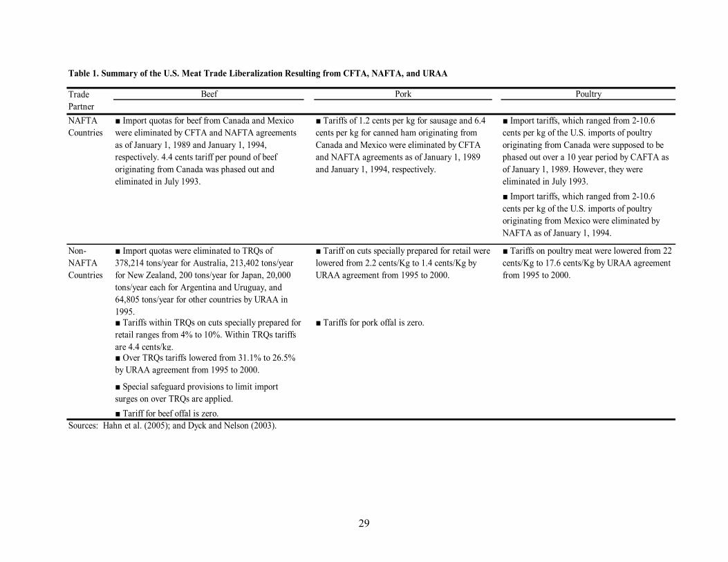
An Overview of U.S. Meat Trade Policies
The U.S. government restricted the importation of meats through a quota system under the 1979
Meat Import Law (MIL). The law required the U.S. president to impose quotas on imports of
beef, veal, mutton, and goat meat when the aggregate annual quantity supplied of such meats had
exceeded a prescribed trigger level (USDHS-CBP, 2005). The quota restriction under MIL was
allocated to various supplying countries on the basis of their historic shares in the U.S. domestic
market. However, the U.S. meat import quotas established under MIL were eliminated
subsequent to the bilateral and multilateral trade agreements between the U.S. and other
5
countries, including the Canada-U.S. Free Trade Agreement (CFTA), the North American Free
Trade Agreement (NAFTA), and the Uruguay Round Agreement on Agriculture (URAA). A
summary of the U.S. meat trade liberalization is presented in table 1.
The U.S. import tariffs for beef, pork, and poultry from Canada and Mexico were totally
eliminated in 1993 by CFTA and in 1994 by NAFTA, respectively. Under the URAA, the U.S.
replaced the import quota system established under MIL with tariff-rate quotas (TRQs) for U.S.
beef imports from non-NAFTA countries (table1). Moreover, special safeguard provisions,
which aim to limit import surges by allowing the U.S. to raise tariffs if the volume of imports
exceeds a certain amount or if the import prices fall by a certain percentage of a base price, are in
effect for U.S. beef imports (Obara, Dyck, and Stout, 2003).
Although significant progress has been made towards liberalization of the U.S. meat
import market, sanitary and phytosanitary (SPS) measures are currently prevalent and constitute
a major form of restricting meat imports. The U.S. banned beef imports from Canada in May
2003 when BSE was detected there. This ban continued until August 2003, when the U.S. lifted
the ban of Canadian boneless beef from cattle less than 30 months of age as cattle of this age are
considered as having little risk of transmitting BSE (Hahn et al., 2005). Furthermore, fresh meats
originating from certain countries such as Mexico and South American countries have not been
allowed to enter the U.S. due to the prevalence of Classical Swine Fever, Exotic Newcastle
(END), Avian Influenza (AI), and foot-and-mouth disease (FMD) in those areas (Hahn et al.,
2005; Leuck, 2001).
A Model of the U.S. Source Differentiated Meat Demand
Although information about source of origin of different meat types is available at the wholesale
level, U.S. meat consumers generally are not given this information at the time of purchase.
6
Therefore, the appropriate theory to derive U.S. source differentiated meat demand seems to be
one based on production theory, with the retailer profit maximization or cost minimization as an
objective, rather than one based on consumer theory. Using a two-stage budgeting procedure (a
profit maximization framework in the first stage and a cost minimization framework in the
second stage), Davis and Jensen (1994) derived a source differentiated demand model of the
form:
(1) ),( gii Xqqhh gp=
where, in this study, hi
q is the volume demanded of meat i from source h; gp is the vector of
prices of source differentiated meats in meat group g; and gX represents the total expenditure on
meat group g.
According to Davis and Jensen (1994), the demand model represented in equation (1) is a
conditional Marshallian constant cost input demand function that can be derived from the second
stage of a two-stage profit maximization problem. As they show and discuss, this second stage
demand function is observationally equivalent to the second stage demand function coming from
a two-stage utility maximization problem.
The Empirical Model
The almost ideal demand system (AIDS) and the Rotterdam model have been frequently used in
the literature in import demand estimations. In this study, the absolute price version of the
Rotterdam model is used to estimate source differentiated meat demands in the U.S. Several past
studies have used the Rotterdam model to estimate demand for source differentiated goods
(Weatherspoon and Seale Jr., 1995; and Seale Jr., Sparks, and Buxton, 1992).
Besides being theoretically reasonable for estimating import demand equations, the
Rotterdam model is advantageous because it can be estimated using linear estimation procedures
7
and the theoretical restrictions can be imposed and tested easily. Furthermore, it also allows for a
theoretically correct specification of exogenous demand shifters with and without imposing
functional restrictions on shift variables (Marsh, Schroeder, and Mintert, 2004).
According to Seale Jr., Sparks, and Buxton (1992) and Marsh, Schroeder, and Mintert
(2004), the absolute price version of the source differentiated Rotterdam model with indicator
variable demand shifters is specified as the following:
(2) ( ) )log(loglog2
1
3
1
*
0 kkhhhmhlhhh j
j
ji
k
im
m
il
l
iiii pdQdDZqdw ∑∑∑∑ ++++===
γβααα
where subscripts i and j indicate goods (beef, pork, and poultry), h and k indicate supply sources
(country of origin), l indicates the number of seasonality indicator variables, and m indicates the
number of the BSE indicator variables. *
hiw is the budget share of good i from source h, here
defined as: 2/)(1
*
−+=
hththt iii www ; hi
q is the quantity demanded of meat i from source h; lZ is a
quarterly indicator variable for seasonality; mD represents the U.S. and Canadian BSE outbreak
indicator variables; Q is the divisia volume index, here defined as )(logloghh i
i h
i qdwQd ∑∑= ;
kjp is the price of meat j from source k (with j including h and k including h), and
0hiα ,
hliα ,
hmiα ,
hiβ , and
kh jiγ are parameters to be estimated; and iii xdxxd /)log( = .
General demand restrictions of homogeneity, symmetry, and adding-up, which are
derived from economic theory, are imposed using parameter constraints as shown in equation
(3), (4), and (5) respectively.
(3) 0=∑∑j h
ji khγ
(4) hkkh ijji γγ =
8
(5) 00=∑∑
i
i
hh
α ; 0=∑∑i
i
hhl
α ; 0=∑∑i
i
hhm
α ; 1=∑∑i
i
hh
β ; 0=∑∑j k
ji khγ
The conditional Cournot (uncompensated) own-price and cross-price elasticities, the conditional
Slutsky (compensated) own-price and cross-price elasticities, and expenditure elasticity are
calculated at the mean level of expenditure shares (Seale, Jr., Sparks, and Buxton, 1992).
The statistical significance of elasticities is determined by the method offered by Mdafri and
Brorsen (1993).3
Statistical tests are performed in the Rotterdam model (equation 2). Specifically, the
assumption of normality of the error terms, joint conditional mean (no autocorrelation, parameter
stability, and linear functional form), and joint conditional variance (static and dynamic
homoskedasticity, and variance stability) are tested using the system misspecification tests as
suggested by McGuirk et al. (1995). Furthermore, various hypotheses regarding the U.S. meat
demand model, including block separability and product aggregation are tested for the U.S.
source differentiated Rotterdam model (equation 2).
Block Separability Test
This study tests block separability within the meat groups. The three different blocks are beef,
pork, and poultry, with each block (for beef and pork since not much poultry is imported in the
U.S.) composed of meats from different sources. The block separability test is used to test if
meat buyers’ preferences within each block can be explained independent of quantities of meats
in the other blocks. More specifically, for parsimonious estimation it is useful to know whether
each block of meat (beef from different sources) could be studied separately from meats in other
blocks (poultry and pork from different sources) without incorporating their prices (not including
the prices of pork and poultry in the beef equations). This study uses quasi-separability of the
cost function to test for separability between blocks (for the test of quasi-separability of the cost
9
function, see Hayes, Wahl, and Williams, 1990, p. 561; Yang and Koo, 1994, p. 400). The null
hypothesis for this test is that each block of meats is separable from all other meat blocks.
Following Hayes, Wahl, and Williams (1990), and Yang and Koo (1994), the restriction to be
tested is given as follows:
(6) ijjiji khkhww γγ ••=
where kh ji
γ is the cross-price parameter between meat i from source h and meat j from source k.
For example, in testing the null hypothesis that the demand for U.S. produced grain-fed beef is
separable from the demand for U.S. produced pork, kh ji
γ is the cross-price parameter between
U.S. produced grain-fed beef and U.S. produced pork. •
hiw is the mean of budget shares of meat i
from source h within the meat group i (the mean of budget shares of U.S. produced grain-fed
beef within the beef group for the above example); •
kjw is the mean of budget shares of meat j
from source k within the meat group j (the mean of budget shares of U.S. produced pork within
the pork group for the above example); and ijγ is the cross-price parameter between groups i and
j, estimated from an aggregate Rotterdam model (the cross-price parameter between beef and
pork under the non-source differentiated Rotterdam model for the above example).
Product Aggregation Test
The source differentiated model used in this study is based on the assumption that meat buyers
place different values on the same meat type originating from different sources. However, this
assumption needs to be tested. The product aggregation test is used to test the restrictions that the
parameters of the source differentiated Rotterdam model are the same as the parameters of the
non-source differentiated Rotterdam model (aggregate model). The null hypothesis for this test is
that each kind of meat can be aggregated (not to be separated by supply source) and estimated
10
using a non-source differentiated Rotterdam model. Non-source differentiation (aggregation)
reduces the number of parameters to be estimated and therefore increases the degrees of
freedom, compared to the non-aggregated models.
Following Yang and Koo (1994), for testing product aggregation (the model that does not
differentiate meats by source of origin) can be done by testing the following restrictions.
(7) ,ihiih∈∀= αα
,,, jikhijji kh∈∀= γγ
.ihiih∈∀= ββ
where hi
α , kh ji
γ , andhi
β are the estimated intercept, own and cross-price parameters, and
expenditure parameters of the source differentiated Rotterdam model presented in equation (2);
iα , ijγ , and iβ are the estimated intercept, own and cross-price parameters, and expenditure
parameters of the non-source differentiated Rotterdam model (aggregate model). For example, in
testing the null hypothesis that beef can be aggregated (non source differentiated), hi
α , kh ji
γ ,
andhi
β are the estimated intercept, own and cross-price parameters, and expenditure parameters
of the source differentiated beef products (U.S. grass-fed beef, U.S. grain-fed beef, Canadian
beef, Australian beef, New Zealand beef, and ROW beef) from equation (2) and iα , ijγ , and iβ
are the estimated intercept, own and cross-price parameters, and expenditure parameters of
aggregate beef (not differentiated by source of supply) from the non-source differentiated
Rotterdam model.
The Wald F-test is used to test the hypothesis of product aggregation over different
supply sources. This test is conducted by imposing restrictions related to the assumption of
product aggregation represented in equation (7) above on the parameters of the source
11
differentiated model (equation 2). If the Wald F-test results indicate the rejection of the null
hypotheses (equation 7), it can be concluded that meat buyers place different values on the same
meat type originating from different sources. Hence, U.S. meat demand should be estimated
using source differentiated models.
Data and Estimation Procedures
Quarterly data from 1995 (quarter I) to 2005 (quarter IV) are used to estimate the parameters of
the U.S. source differentiated meat demand. For this study, 1995 is chosen for the beginning of
data because the major U.S. meat import barrier (import quota system) was eliminated in 1995.
This is also the year that the URAA began to be implemented. The meats studied here are beef,
pork, and poultry. Beef from the U.S. is differentiated by quality (grain-fed and grass-fed), and
beef and pork are differentiated based on the origin of supply (source differentiated).4 A country
is identified as a supply source if imports from that source constituted at least 10% of the total
imports of the selected meat. All other sources that supplied less than 10% of the U.S. total
imports of the selected meat are aggregated as the ROW. Using this criterion, U.S. meat imports
are categorized as: beef from Australia, beef from Canada, beef from New Zealand, beef from
the ROW, pork from Canada, and pork from the ROW. Poultry is not differentiated by supply
source, since more than 95% of U.S. poultry consumption is supplied by U.S. producers.
Because retail prices for source differentiated meats in the U.S. are not available, unit-
value import prices are used to measure market prices for imported meats.5 Source differentiated
import prices (unit values) of individual meats are calculated by dividing the total import values
by the total import quantities. Data on import values (in thousand of U.S. dollars) and quantities
(in metric tons) are from USDA-FAS, 2006. Data on U.S. domestic meats at the wholesale level
are from various sources. For U.S. produced beef and pork, quantity and price data are from
12
USDA-ERS, 2006a, and data for poultry are from USDA-ERS, 2006b. The quantity of grain-fed
beef is calculated as the sum of the quantities demanded of beef from steers and heifers. The
quantity demanded of grass-fed beef is calculated as the sum of the quantity demanded of beef
from cows and bulls. Slaughter steer price of choice 2-4 Nebraska Direct is used as the price of
grain-fed beef. Slaughter cutter cow price is used for the price of grass-fed beef.
Seasonal and BSE indicator variables are included in the Rotterdam model to measure the
impact of seasonality and BSE disease outbreaks on the U.S. meat demand. Three seasonal
quarterly variables are included for the first (January through March), third (July through
September), and fourth (October through December) quarters. Two BSE dummy variables, one
accounting for the BSE outbreak in Canada and another accounting for the BSE outbreak in the
U.S. are included in the model. The BSE indicator variables are intended to reflect the period
during which the BSE scare in the U.S. would have been most likely to occur. It is assumed here
that if the BSE outbreak would have had any impact on the U.S. meat demand, it would have
been during the period when NAFTA countries banned beef imports from the North American
infected countries. Therefore, the BSE indicator variables take the value of one during the beef
import ban periods in other NAFTA countries. On the other hand, the lifting of the import ban by
the NAFTA countries may have signaled the respective governments’ confidence regarding the
safety of beef to the U.S. meat buyers. We assume that the U.S. meat buyers may not have
necessarily reacted in the same way to bans by (not nearby) countries in other continents, such as
Japan and S. Korea. More specifically; U.S. and Japanese consumers are reported to react
differently in terms of their meat demand to non-price and non-income concerns, including food
safety issues (Tonsor and Marsh, 2007). Hence, the period during which Japan and South Korea
13
banned U.S. and Canadian beef is not considered in constructing the BSE dummy variables used
in the U.S. source differentiated meat demand.
Although media coverage indices have been used to model demand response to food
scares (Piggott and Marsh 2004), this study uses indicator variables. Empirical applications of
media coverage indices in modeling demand response to food scares have some important
limitations. These shortcomings may be a result of the subjective nature of consumers’
discrimination between positive and negative information; depreciation of the information effect
due to the memory discount effect; and the differing effect of confirmatory news from the first
news (Mazzocchi, 2006). Furthermore, collecting and analyzing adequate media coverage
information can be a time-consuming and potentially an expensive operation. Hence, since the
period when NAFTA countries banned beef imports from the North American infected countries
is known, this study uses the BSE indicator variables.
The U.S. import ban on Canadian beef began in May 2003 and lasted through August
2003 when the ban of Canadian beef from cattle younger than 30 months of age was lifted in
NAFTA countries (Hahn et al., 2005). Consequently, the Canadian BSE outbreak indicator
variable takes the values of one for the second and the third quarters of the year 2003 and zero at
other times. Similarly, the ban on U.S. beef from NAFTA countries began in December 2003
and lasted through March 2004, when NAFTA countries lifted the ban of U.S. beef from cattle
younger than 30 months of age (Hahn et al., 2005). Therefore, the U.S. BSE outbreak indicator
variable takes the values of one for the fourth quarter of the year 2003 and the first quarter of the
year 2004 and zero at other times.
Animal disease outbreaks in Mexico and in South American countries such as Brazil,
Argentina, and Uruguay have been frequently documented. However, animal disease outbreak
14
variables for these countries are not included in this study. They are omitted because none of
these countries is a separate source of meat supply in the model used in this study (all are
included in the ROW). Additionally, Hahn et al. (2005) report that the majority of U.S. imports
from these countries are composed of highly processed or cooked meats that are sealed in air-
tight containers. Because of this fact, these meats may be perceived as safe. Therefore, animal
disease outbreaks in these countries might not significantly impact the U.S. meat demand.
The iterative seemingly unrelated regression (ITSUR) estimation method is used to
estimate the parameters of the Rotterdam model (equation 2).6 Due to the adding-up condition,
the contemporaneous covariance matrix is singular. Therefore, one equation (pork from the
ROW equation) is dropped from the system for estimation purposes. If the maximum likelihood
estimation method is used, the resulting estimates are invariant to which equation is dropped.
Because the ITSUR estimations for the complete demand systems are equivalent to the
maximum likelihood estimates, the parameters estimated in this study are invariant to which
equation is dropped. The theoretical restrictions of symmetry, adding up, and homogeneity are
imposed to make the model consistent with economic theory.
Results
Prior to the estimation of the parameters of the U.S. source differentiated Rotterdam model
(equation 2); the appropriateness of the model was tested using the system misspecification tests
as described in the Model section. Results of the system misspecification tests are presented in
table 2. Test results indicate the failure to reject the null hypothesis of normality of the error
terms at the 1% significance level. Results of the Joint conditional mean and joint conditional
variance tests indicate the rejection of the null hypotheses that the joint conditional mean and
joint conditional variance are properly specified at the 1% significance level. This might be due
15
to the autocorrelation of the error terms which test results confirm in this study (table 2).
Dynamics are expected to be particularly important in the analysis of the U.S. meat demand
system as meat buyers are unlikely to respond fully to changes in price, income, or other
determinants of demand in the short run. Psychological factors (consumption habits), inventory
adjustments, or institutional factors have been given as reasons for the lagged consumer response
(Kesavan et al., 1993; Henneberry and Hwang, 2007). Therefore, to allow for the lagged effects,
the final model is estimated using iterative seemingly unrelated regression, corrected for
autocorrelation (Berndt and Savin, 1975; and Piggott and Marsh, 2004).
Block separability and product aggregation tests were also conducted by imposing the
restrictions related to block separability and product aggregation assumptions on the final model
(corrected for autocorrelation), following the description given in the Model section for these
tests. Test results of the null hypotheses of block separability among the included meats (table 2)
indicate the rejection of the null hypotheses at the 1% significance level. Therefore, test results
support estimating the U.S. source differentiated Rotterdam model for meats, including all three
types of meats. Furthermore, test results presented in table 2 indicate that the null hypothesis of
non-source differentiation (product aggregation) for all meats is rejected at the 1% significance
level. Hence, the results support estimating U.S. demand for meats, using a source differentiated
model.
Calculated Marshallian (uncompensated cournot) and Hicksian (compensated slutsky)
demand elasticities with their standard errors in parenthesis are presented in tables 3 and 4,
respectively. Estimated parameters of seasonal and BSE indicator variables are also presented in
table 3. Of importance to note is that the results discussed in the following sections represent
16
U.S. demand for domestically produced and imported meats, estimated using wholesale level
data.
Price and Expenditure Elasticities
Consistent with economic theory, all source differentiated own-price elasticities are negative and
statistically significant (tables 3 and 4). In the beef market, most own-price elasticities fall within
the range of -0.15 to -2.59. This range is consistent with published own-price elasticities for beef
reported by the U.S. Environmental Protection Agency (USEPA). The estimated own-price
elasticities of imported beef from Australia and New Zealand are greater than 2.6 in absolute
value (tables 3 and 4). These results suggest that imported beef from major grass-fed beef
suppliers are sensitive to own-price in the U.S. domestic market. These results support the
findings from previous studies that the perceived lower quality meats (such as grass-fed beef
imported from Australia and New Zealand) have higher own-price elasticities, compared to
perceived higher-quality meats (grain-fed beef from the U.S. and Canada) (Lusk et al, 2001;
Brester and Wohlgenant, 1991; and Eales and Unnevehr, 1988). Similar to beef, in the pork and
poultry markets, most of the calculated own-price elasticities are less than one and fall within the
range of -0.070 to -1.234 for pork and -0.104 to -1.250 for poultry, as reported by USEPA.
The compensated (Hicksian) cross-price elasticities (table 4) indicate net substitutability
or net complementary relationships among products from different sources. While a significant
positive Hicksian cross-price elasticity between meats from different suppliers may indicate
substitutability, a significant negative cross-price elasticity may indicate complementary
relationship. Justifying a complementary relationship between meats is difficult since all meats
are sources of animal protein and therefore are expected to substitute for one another in human
consumption.
17
For the U.S. beef market, the results show that U.S. grain-fed beef is a net substitute to
beef from various sources, especially with U.S. grass-fed beef and imported beef from Canada
and New Zealand (first row, table 4). The substitutability between U.S. grain-fed beef with U.S.
grass-fed beef and beef from New Zealand is an unexpected result because of the difference in
quality between U.S. grain-fed beef with these beef products. However, the substitutability
relationship between U.S. grain-fed beef and Canadian beef is consistent with prior expectations
since both beef products are produced from grain-fed cattle of similar quality. Moreover, the
magnitude and statistical significance of cross-price elasticities indicate that while the demand
for U.S. grain-fed beef is not strongly impacted by the prices of imported beef and U.S. grass-fed
beef (first column, table 4), the price of U.S. grain-fed beef has a more noticeable impact on the
demand for other beef products (first row, table 4).
Regarding other suppliers, beef from New Zealand and Australia show to be substitutes.
The substitutability between the imported beef from Australia and New Zealand is consistent
with prior expectations, since both countries supply beef from grass-fed cattle to the U.S. beef
market. Substitutability also exists between Canadian beef and ROW beef. The U.S. beef imports
from the ROW (mainly South American countries) are mainly composed of further processed,
grass-fed beef products due to the prevalence of animal diseases (mainly foot-and-mouth
disease) in those countries. Hence, the substitutability between Canadian beef and ROW beef
might be consistent with previous expectations because the further processed (value added) beef
from the ROW might be perceived by U.S. meat buyers as having a similar value compared to
grain-fed Canadian beef. However, Canadian beef shows a statistically significant
complementary relationship with U.S. grass-fed and New Zealand beef. Again, these results are
consistent with prior expectations since the U.S. imports of beef from Canada are mainly
18
composed of high-quality beef cuts graded as choice and select from grain-fed cattle. The choice
and select quality beef are not expected to compete with U.S. grass-fed beef mainly from cows
and bulls and New Zealand grass-fed beef (used mostly for hamburger meat).
Regarding the pork market, the estimated cross-price elasticities show that U.S. pork
competes with pork from Canada. However, ROW pork shows a complementary relationship
with U.S. and Canadian pork. The lack of substitutability might be due to differences in meat
cuts and products between pork from North America (the U.S. and Canada) and pork from the
ROW. While Canada and the U.S. produce similar quality pork products, mainly composed of
whole pork carcasses; the U.S. imports from the ROW are mainly composed of spare ribs and
hams from Denmark.
Regarding cross-meat products relationships (e.g., the relationship between source
differentiated beef and source differentiated pork), the results show a substitution relationship
between U.S. pork on one hand and U.S. grain-fed, U.S. grass-fed beef, and Canadian beef on
the other hand. Moreover, Canadian pork shows a substitute relationship with beef from Canada,
Australia, and the ROW. There is no clear relationship between U.S. poultry and source
differentiated beef and pork products since the majority of cross-price elasticities are not
statistically significant. In the Summary and Conclusions section, the discussion will address the
implications of these relationships.
Regarding expenditure elasticities in the beef market; all expenditure elasticities are
positive (table 3). Moreover, the expenditure elasticity estimates of U.S. grain-fed beef and
Canadian beef (which is mainly composed of grain-fed beef) are greater than one. These
estimates being greater than one are consistent with U.S. consumers’ preferring grain-fed beef
from the U.S. and Canada, over grass-fed beef imported from Australia and New Zealand and
19
U.S. grass-fed beef. Moreover, the estimated expenditure elasticity of Canadian beef (2.451) is
higher than that of U.S. grain-fed beef (1.258). Consequently, a Wald-F test was conducted to
test the hypothesis of the two elasticities being equal. Test results (p-value = 0.744) failed to
reject the null hypothesis that the two elasticities are equal. This failure to reject the equality of
the two elasticities is at least partially due to the imprecision in estimating the Canadian
expenditure elasticity, which is not significantly different from zero.
Regarding the pork market, all expenditure elasticities are positive; however, only the
expenditure elasticity of U.S. pork is statistically significant. The U.S. demand for ROW pork is
expenditure elastic (1.391). This result is consistent with the general preferences for pork in the
U.S. since U.S. pork imports from the ROW are mainly composed of high quality spare ribs and
hams from Denmark, which are preferred by U.S. consumers (USDA-ERS, 2006c). In the
poultry market, the expenditure elasticity of U.S. poultry is positive, greater than one, and
statistically significant.
Effects of Seasonality and BSE on the U.S. Meat Demand
The parameter estimates of seasonal and BSE indicator variables are presented in table 3. In the
beef market, the coefficients of seasonal indicator variables show that the budget shares of most
of the beef products (U.S. grain-fed beef, Australian beef, and New Zealand beef) are lower in
the fourth quarter compared to the second quarter. These results are consistent with seasonal
consumption patterns in the U.S.: the fourth quarter (October-December) is associated with
traditional holiday seasons when Americans consume more poultry meat than beef compared to
other seasons. In the pork market, the results of the seasonal indicator variables show that the
shares of pork from different sources are higher in the fourth quarter compared to the second
quarter. Since most of the pork consumption in the U.S. is in the form of breakfast meats, the
20
consumption of pork is expected to decrease during the warm summer months (second quarter).
This is consistent with prior expectations because consumers are more likely to eat hot breakfasts
during the colder seasons.
Regarding BSE impacts, the results indicate that the BSE outbreak in Canada did not
affect the source differentiated meat shares in the U.S. However; the BSE outbreak in the U.S.
decreased the shares of U.S. grass-fed beef and increased the shares of Canadian and ROW beef.
The negative impact of the U.S. BSE outbreak on the U.S. grass-fed beef market share is
consistent with previous expectations because U.S. grass-fed beef, which is composed of cows
and bulls, is considered to carry a higher risk of transmitting BSE. Similarly, the results that the
U.S. BSE outbreak increased the shares of Canadian and ROW beef are consistent with previous
expectations. This increase might have resulted from meat buyers substituting beef from those
import sources, which were perceived safe by U.S. consumers, for U.S. grass-fed beef during the
U.S. BSE outbreak.7
Summary and Conclusions
This study estimates the impacts of economic factors (meat prices and expenditure) and non-
economic factors (seasonality and BSE outbreaks in the U.S. and Canada) on the U.S. quantity
demanded for source differentiated meats, using the absolute price version of the Rotterdam
model. To assure that the system specification and estimation procedures were correct, various
hypotheses regarding the U.S. source differentiated meat demand model were tested. The tested
hypotheses include: normality, joint conditional mean, joint conditional variance, separability
among meats included in the system, and product aggregation. The results of misspecification
tests show that the joint conditional mean and joint conditional variance is not well specified,
mainly due to autocorrelation of the error terms. Hence, the model was estimated using iterative
21
seemingly unrelated regression with autocorrelation correction. Moreover, the results of
statistical tests support estimating a set of meat demand equations for the three types of meats
(beef, pork, and poultry), each meat being differentiated by the supply source (source
differentiated).
This study is one of the first that analyzes source differentiated meat demand in the U.S.
domestic market. The results of this study shed light on the preferences for meats from different
sources, including domestically produced meats in the U.S. meat market. Furthermore, the
impacts of seasonality and the BSE outbreaks in the U.S. and Canada on the U.S. demand for
source differentiated meats are analyzed. The estimated price and expenditure elasticities are
used to access the competitiveness of U.S. produced meats in the U.S. domestic market.
Following the definition of competitive advantage, the results of this study indicate that
U.S. grain-fed beef has competitive advantage in the U.S. market, compared to beef from other
major supplying sources. This is judging by its relatively small own-price elasticity (in absolute
values) and greater than one and statistically significant expenditure elasticity, compared to beef
from other major suppliers. In the pork market, similar to beef, U.S. produced pork has
competitive advantage compared to pork from other sources. This is because the expenditure
elasticity of U.S. pork is statistically significant and the own-price elasticity of U.S. pork is the
lowest (in absolute value) among own-price elasticities of pork from other sources.
The results of this study would have implications for the global meat suppliers to the U.S.
market in the event of market condition changes, free trade agreements, and animal disease
outbreaks. For example, if the increased availability of Australian beef in the U.S. resulting from
the 2005 U.S./Australia free trade agreement reduces the relative price of Australian beef and
considering the large positive and statistically significant New Zealand/Australia cross-price
22
elasticities, New Zealand producers are expected to have the most to lose in terms of decreased
exports and reduced U.S. market shares.
Another current application of this study is the implication of animal disease outbreaks
on the meat share of various suppliers in the U.S. market. The substitute relationship of U.S.
produced pork with U.S. and Canadian-produced beef may indicate that the demand for U.S.
pork might increase following a cattle disease such as the BSE outbreak in North America.
Finally, market development activities intended to increase meat consumption in the U.S. are
expected to have the most significant impact (in terms of percentage change in sales volume) on
U.S. and Canadian grain-fed beef, ROW pork, and U.S. poultry) compared to other meat
products.
23
Footnotes
1. Competitive advantage may be defined as an advantage over competitors gained by offering
meat buyers a greater value; either by lowering prices or by providing greater benefits and
services, such as high-quality products that justify higher prices (Porter, 1985). In this study, any
meat product that carries a higher and statistically significant expenditure elasticity compared to
other meats is assumed to be perceived by meat buyers as a higher value product. Furthermore,
suppliers that supply higher-valued meat products would be expected to prefer facing an own-
price inelastic demand. This is because the higher prices associated with their meats, compared
to other meats from other suppliers, will result in an increase in their total revenues (ceteris
paribus). Therefore, in this study, a country that supplies higher-priced meat products, such as
the U.S., is said to have a competitive advantage in a market that has a price-inelastic and
expenditure elastic demand.
2. In this study, the ROW refers to the group of all other countries that export a specific type of
meat to the U.S., except those countries which are analyzed in this study and identified as the
U.S. competitors. For example, ROW beef is beef that the U.S. imports from all other countries
except for Australia, Canada, and New Zealand.
3. The equations of own-price, cross-price, and expenditure elasticities can be written in matrix
form as Abe = where e is the vector of estimated elasticities (ε ’s and η ’s); b is the vector of
estimated Rotterdam model parameters (γ ’s and β ’s); and A is a matrix of constants (budget
shares). The standard errors are calculated by taking the square root of the variance covariance
matrix of e [VAR( e ), given by 'VAR( ) VAR( )e A b A= where VAR(b ) is the variance
covariance matrix of b].
24
4. Due to a lack of disaggregated trade data, this study implicitly assumes that each type of meat
from the same source is a relatively homogeneous product. This assumption might be okay
because the meat exporting countries to the U.S. mainly specialize in exporting specific meat
categories. For example, the majority of U.S. beef imports from Australia and New Zealand are
composed of mainly grass-fed beef, while Canadian exports to the U.S. are mainly composed of
grain-fed beef. However, some aggregation bias might still exist from the homogeneity
assumption, which results from the actual differences in meat categories (cuts and organs) within
each source differentiated meat.
5. Although unit values usually reflect perceived quality differences of imported meats, they may
differ from wholesale prices when trade restrictions are in effect.
6. The U.S. meat demand system was also estimated using a linear as well as a non-linear version
of the AIDS model. While the linear approximation of the AIDS model (LA/AIDS) produced
elasticities that were similar in magnitude and signs to the calculated elasticities using the
Rotterdam model, the non-linear AIDS model did not converge. Convergence failure of the non-
linear AIDS model is expected in cases where a large number of parameters need to be estimated
using a limited number of observations (44 here).
7. Although there was a BSE outbreak in Canada in May 2003, prior to the U.S. BSE outbreak in
December 2003, Canadian beef might have been considered safe by the U.S. consumers. This is
because the U.S. government had already lifted the ban on Canadian fresh beef products from
cattle younger than 30 months of age as of August 2003, signaling the safety of Canadian beef to
the U.S. consumers (Hahn et al., 2005).
25
References
Berndt, E.R. and N.E. Savin. “Estimation and Hypothesis Testing in Singular Equation Systems
with Autoregressive Disturbances.” Econometrica 43(1975):937-958.
Brester, G.W., M.K. Wohlgenant. “Estimating Interrelated Demands for Meats Using
New Measures for Ground and Table Cut Beef.” American Journal of Agricultural
Economics 73(November 1991): 1182-1194.
Davis, G.C. “Product Aggregation Bias as a Specification Error in Demand Systems.” American
Journal of Agricultural Economics 79 (February, 1997): 100-109.
Davis, G.C. and K.L. Jensen. “Two-Stage Utility Maximization and Import Demand Systems
Revisited: Limitations and an Alternative.” Journal of Agricultural and Resource
Economics 19(1994): 409-424.
Dyck, J.H. and K.E. Nelson. “Structure of the Global Markets for Meat.” Agricultural Bulletin
Number 785.USDA/Economic Research Service, Washington, DC, September 2003.
Eales, J.S., and L.J. Unnevehr. “Demand for Beef and Chicken Products: Separability
and Structural Change.” American Journal of Agricultural Economics 70(August 1988):
521-532.
Hahn, W.F., M. Halley, D. Leuck, J.J. Miller, J. Perry, F. Taha, and S. Zahniser. ”Market
Integration of the North American Animal Product Complex.” Electronic Outlook
Report. USDA/Economic Research Service, Washington DC, May 2005.
Hayes, D.J., T.I. Wahl, and G.W. Williams. “Testing Restrictions on a Model of
Japanese Meat Demand.” American Journal of Agricultural Economics 72(August
1990): 556-566.
Henneberry, S.R. and S-K. Hwang. “Meat Demand in South Korea: An Application of
26
the Restricted Source Differentiated AIDS Model.” Journal of Agricultural and Applied
Economics 39 (April 2007): 47-60.
Jones, K.G., W.F. Hahn, and C. G. Davis. “Demand for U.S. Lamb and Mutton by
Country of Origin: A Two-Stage Differential Approach. Selected Paper, American
Agricultural Economics Association, Canada, July 27-30, 2003.
Kesavan, T., Z.A. Hassan, H.H. Jensen, and S.R. Johnson. “Dynamic and Long-run
Structure in U.S. Meat Demand.” Canadian Journal of Agricultural Economics
41(1993):139-53.
Leuck, D. The New Agricultural Trade Negotiations: Background and Issues for the
U.S. Beef Sector.” Electronic Outlook Report. USDA/Economic Research Service,
Washington DC, December 2001.
Lusk, J.L., T.L. Marsh, T.C. Schroeder, and J.A. Fox. “Wholesale Demand for USDA
Quality Beef and Effects of Seasonality.” Journal of Agricultural and Resource
Economics 26 (2001): 91-106.
Marsh, T.L, T.C. Schroeder, and J. Mintert. “Impacts of Meat Product Recalls on Consumer
Demand in the USA.” Journal of Applied Economics 36 (2004): 897-909.
Mazzocchi, M. “No News Is Good News: Stochastic Parameters versus Media Coverage Indices
in Demand Models After Food Scares.” American Journal of Agricultural Economics 88
(2006): 727-741.
McGuirk, A., P. Driscoll., J. Alwang., and H. Huang. “System Misspecification Testing
and Structural Change in the Demand for Meats.” Journal of Agricultural and Resource
Economics 20(1995): 1-21.
Mdafri, A. and B.W. Brorsen. “Demand for Red Meat, Poultry, and Fish in Morocco: An
27
Almost Ideal Demand System.” Agricultural Economics 9(1993): 155-163.
Muhammad, A., K.G. Jones, and W.F. Hahn. “U.S. Demand for Imported Lamb by
Country: A Two-Stage Differential Production Approach. Selected Paper, Southern
Agriculture Economics Association, Tulsa, OK, February 14-18, 2004.
Obara, K., J. Dyck, and J. Stout. “Pork Policies in Japan.” Electronic Outlook Report. USDA/
Economic Research Service, Washington DC, March 2003.
Piggott, N.E. and T.L. Marsh. “Does Food Safety Information Impact U.S. Meat
Demand?” American Journal of Agricultural Economics 86 (February 2004):154-174.
Porter, M.E. “Competitive Advantage. Creating and sustaining superior performance.”
Macmillan Inc. London 1985.
Seale Jr., J.L., A.L. Sparks, and B.M. Buxton. “A Rotterdam Application to International Trade
in Fresh Apples: A Differential Approach.” Journal of Agricultural and Resource
Economics 17(1992): 138-149.
Tonsor, G.T. and T.L. Marsh. “Comparing Heterogeneous Consumption in U.S. and Japanese
Meat and Fish Demand.” Agricultural Economics 37 (2007): 81-91.
United States Department of Homeland Security/ Customs & Border Protection (USDHS-CBP).
“SEC.321.Agriculture.” Internet site: http://www.cbp.gov/nafta/nafta048.htm. (Accessed
in December 2005).
United States Department of Agriculture/Economic Research Service (USDA-ERS). Briefing
Rooms, Animal Production and Marketing Issues: Trade. Internet site:
(http://www.ers.usda.gov/Briefing/AnimalProducts/Trade.htm, (Accessed: April 2007.
____.“Red Meat Yearbook.” Internet site:
28
http://www.ers.usda.gov/Data/sdp/view.asp?f=livestock/94006/. (Accessed in May
2006a).
____. “Poultry Yearbook.” Internet site:
http://www.ers.usda.gov/data/sdp/view.asp?f=livestock/89007/. (Accessed in August
2006b).
____. “Briefing Rooms, Hog: Trade.” Internet site:
http://www.ers.usda.gov/Briefing/Hogs/Trade.htm. (Accessed July 2006c).
United Stated Department of Agriculture/Foreign Agriculture Service (USDA-FAS).
“Foreign Agriculture Trade of United Sates Data Base.” Internet site:
http://www.fas.usda.gov/ustrade/. (Accessed May, 2006).
____. “Livestock and Poultry: World Markets and Trade.” Internet site:
http://www.fas.usda.gov/dlp/circular/2005/05-04LP/toc.htm. (Accessed July 2005).
United States Department of Environmental Protection Agency (USEPA). Economic Analysis of
Proposed Effluent Limitations Guidelines and Standards for the Meat and Poultry
Products Industry. EPA-821-B-01-006, Washington DC, 2002.
Weatherspoon, D.D. and J.L. Seale Jr. “Do the Japanese Discriminate Against Australian Beef
Imports?: Evidence From the Differential Approach.” Journal of Agricultural and
Applied Economics 27 (December 1995): 536-543.
Yang, S-R. and W.W. Koo. “Japanese Meat Import Demand Estimation with the Source
Differentiated AIDS Model.” Journal of Agricultural and Resource Economics 19
(1994): 396-408.
29
Beef Pork Poultry
■ Import tariffs, which ranged from 2-10.6
cents per kg of the U.S. imports of poultry
originating from Canada were supposed to be
phased out over a 10 year period by CAFTA as
of January 1, 1989. However, they were
eliminated in July 1993.
■ Import tariffs, which ranged from 2-10.6
cents per kg of the U.S. imports of poultry
originating from Mexico were eliminated by
NAFTA as of January 1, 1994.
Non-
NAFTA
Countries
■ Import quotas were eliminated to TRQs of
378,214 tons/year for Australia, 213,402 tons/year
for New Zealand, 200 tons/year for Japan, 20,000
tons/year each for Argentina and Uruguay, and
64,805 tons/year for other countries by URAA in
1995.
■ Tariff on cuts specially prepared for retail were
lowered from 2.2 cents/Kg to 1.4 cents/Kg by
URAA agreement from 1995 to 2000.
■ Tariffs within TRQs on cuts specially prepared for
retail ranges from 4% to 10%. Within TRQs tariffs
are 4.4 cents/kg.
■ Tariffs for pork offal is zero.
■ Over TRQs tariffs lowered from 31.1% to 26.5%
by URAA agreement from 1995 to 2000.
■ Special safeguard provisions to limit import
surges on over TRQs are applied.
■ Tariff for beef offal is zero.
Trade
Partner
Table 1. Summary of the U.S. Meat Trade Liberalization Resulting from CFTA, NAFTA, and URAA
Sources: Hahn et al. (2005); and Dyck and Nelson (2003).
NAFTA
Countries
■ Import quotas for beef from Canada and Mexico
were eliminated by CFTA and NAFTA agreements
as of January 1, 1989 and January 1, 1994,
respectively. 4.4 cents tariff per pound of beef
originating from Canada was phased out and
eliminated in July 1993.
■ Tariffs of 1.2 cents per kg for sausage and 6.4
cents per kg for canned ham originating from
Canada and Mexico were eliminated by CFTA
and NAFTA agreements as of January 1, 1989
and January 1, 1994, respectively.
■ Tariffs on poultry meat were lowered from 22
cents/Kg to 17.6 cents/Kg by URAA agreement
from 1995 to 2000.
30
Hypothesis Tested P-value
System Misspecification Tests
Normality Test
Grain-fed beef from the U.S. 0.4927
Grass-fed beef from the U.S. 0.4927
Beef from Australia 0.0414
Beef from Canada 0.5439
Beef from New Zealand 0.8721
Beef from the ROW 0.6813
Pork from the U.S. 0.4967
Pork from Canada 0.5963
Pork from the ROW 0.8807
Poultry from the U.S. 0.4506
Joint Conditional Mean Test
H0: Linear Functional form 0.0001
H0: No autocorrelation 0.0004
H0: No structural changes 0.8953
H0: Overall Joint conditional mean test 0.0001
Joint Conditional Variance Test
H0: Static homeskedasticity 0.0001
H0: Dynamic homoskedasticity 0.1189
H0: No structural changes 0.8318
H0: Overall joint conditional variance test 0.0001
Block Separability and Product Aggregation Testsa
Block Separability Test
H0: Beef is separable from all other meats 0.0001
H0: Pork is separable from all other meats 0.0001
H0: Poultry is separable from all other meats 0.0001
H0: Overall block separability test 0.0001
Product Aggregation Test
H0: Beef can be aggregated 0.0001
H0: Pork can be aggeregated 0.0001
H0: Overall product aggegation test 0.0001
Note: The null hypothesis for the normality test is that the error terms of each equation are normally distributed.a Block separability and product aggregation tests were performed using a model corrected for autocorrelation
Table 2. Misspecification Test Results for the U.S. Source Differentiated Meat Demand Using Rotterdam Model
31
Explanatory Poultry
Variables U.S. grain-fed U.S. grass-fed Canada Australia New Zealand ROW U.S. Canada ROW U.S.
U.S. grain-fed beef price -0.712** 0.463* -0.542 -0.073 1.465 -0.066 -0.169** -0.256 0.757 -0.322**
(0.120) (0.218) (1.716) (1.068) (0.905) (0.520) (0.062) (0.284) (2.335) (0.081)
U.S. grass-fed beef price 0.016 -0.507** -1.286 0.097 0.426 0.299 0.038* -0.314* -1.464 -0.079**
(0.02) (0.138) (1.169) (0.572) (0.683) (0.333) (0.02) (0.174) (1.337) (0.017)
Canadian beef price -0.004 -0.314 -1.535** 0.043 -0.200 0.539 0.044* 0.024 0.603 0.017
(0.041) (0.306) (0.757) (0.436) (0.382) (0.220) (0.023) (0.113) (1.394) (0.025)
Australian beef price -0.005 0.028 0.020 -2.747** 3.373** 0.001 -0.030 0.955** 0.613 -0.031*
(0.013) (0.121) (0.359) (1.086) (1.214) (0.495) (0.022) (0.314) (1.639) (0.016)
New Zealand beef price 0.025* 0.065 -0.120 2.261** -4.057** 0.161 -0.005 -0.737* 0.742 -0.023**
(0.013) (0.097) (0.211) (0.808) (1.356) (0.447) (0.016) (0.316) (1.095) (0.009)
ROW beef price -0.003 0.041 0.249* 0.000 0.142 -1.285** -0.021** 0.258* 0.231 -0.011**
(0.007) (0.041) (0.107) (0.289) (0.394) (0.262) (0.007) (0.121) (0.501) (0.004)
U.S. pork price -0.266** 0.382* 0.556 -0.897 -0.210 -1.010* -0.468** 1.378** -1.139 -0.306
(0.071) (0.157) (1.133) (0.813) (0.781) (0.417) (0.04) (0.345) (1.640) (1.054)
Canadian pork price -0.013* -0.060* 0.001 0.896** -1.035** 0.409* 0.044** -1.096* -1.640** -0.008
(0.006) (0.035) (0.094) (0.293) (0.442) (0.192) (0.009) (0.279) (0.404) (0.023)
ROW pork price 0.010 -0.129 0.203 0.261 0.147 0.535 -0.014 -0.735** -0.844* 0.016
(0.028) (0.122) (0.480) (0.693) (0.692) (0.360) (0.024) (0.183) (0.448) (0.019)
U.S. poultry price -0.306** -0.253* 0.003 -0.830 -0.867 -0.457 -0.226** -0.125 -1.334 -0.297**
(0.070) (0.143) (1.108) (0.740) (0.586) (0.345) (0.039) (0.179) (2.301) (0.062)
Expenditure 1.258** 0.285 2.451 0.990 0.816 0.874 0.805** 0.648 1.391 1.043**
(0.223) (0.427) (3.593) (2.214) (1.712) (1.021) (0.120) (0.55) (1.230) (0.186)
Quarter I -0.0039 0.0040 0.0056 -0.0036 0.0031** -0.0003 0.0051 -0.0001 0.0005 -0.0087
(0.007) (0.002) (0.004) (0.002) (0.001) (0.001) (0.003) (0.0005) (0.0005) (0.005)
Quarter III -0.0157** 0.0034* 0.0026 -0.0024 -0.0042** 0.0003 0.0231** 0.0016 0.0003 -0.0077
(0.006) (0.002) (0.003) (0.002) (0.001) (0.0004) (0.003) (0.0004) (0.0004) (0.004)
Quarter IV -0.0392** 0.0055** 0.0058* -0.0051** -0.0052** -8.5557E-06 0.0392** 0.0017** 0.0011** -0.0044
(0.005) (0.001) (0.003) (0.002) (0.001) (0.0004) (0.003) (0.0003) (0.0004) (0.003)
BSE in Canada 0.0042 -0.0006 -0.0043 -0.0006 -0.0007 0.0002 -0.0021 -0.0003 -2.3363E-05 0.0004
(0.006) (0.002) (0.004) (0.002) (0.001) (0.0005) (0.003) (0.0004) (0.0004) (0.004)
BSE in the U.S. -0.0127 -0.0077** 0.0113* -0.0003 0.0006 0.0018* 0.0043 -0.0005 0.0003 -0.0056
(0.008) (0.002) (0.005) (0.002) (0.001) (0.001) (0.003) (0.0004) (0.0006) (0.005)
Beef Pork
Table 3. Uncompensated Cournot Price and Expenditure Elasticities, and Seasonality and BSE Impacts, U.S. Mead Demand, Using Rotterdam Model, 1995I-2005IV
Notes: Numbers in parenthesis are asymptotic standard errors. Single (*) and double (**) asterisks denote significance at 5% and 1% level respectively.
32
Explanatory Poultry
Variables U.S. grain-fed U.S. grass-fed Canada Australia New Zealand ROW U.S. Canada ROW U.S.
U.S. grain-fed beef price -0.271** 0.563** 0.316** 0.274 1.751** 0.240 0.113** -0.029 1.244 0.044
(0.091) (0.164) (0.128) (0.747) (0.660) (0.381) (0.044) (0.204) (2.294) (0.047)
U.S. grass-fed beef price 0.075** -0.494** -1.173** 0.143 0.464 0.339 0.075** -0.284* -1.400 -0.030*
(0.022) (0.135) (0.128) (0.559) (0.671) (0.327) (0.019) (0.173) (1.335) (0.014)
Canadian beef price 0.011 -0.311 -1.505** 0.055 -0.190 0.550** 0.054** 0.032 0.621 0.030
(0.041) (0.306) (0.084) (0.437) (0.384) (0.220) (0.023) (0.113) (1.394) (0.025)
Australian beef price 0.008 0.031 0.044 -2.737** 3.381** 0.009 -0.022 0.962** 0.627 -0.021
(0.021) (0.120) (0.039) (1.079) (1.208) (0.492) (0.022) (0.312) (1.638) (0.015)
New Zealand beef price 0.033** 0.067 -0.103** 2.268** -4.052** 0.167 0.001 -0.733* 0.239 -0.016*
(0.013) (0.097) (0.023) (0.810) (1.359) (0.448) (0.016) (0.317) (1.096) (0.008)
ROW beef price 0.004 0.043 0.264** 0.005 0.147 -1.280** -0.016* 0.262* 0.751 -0.005
(0.006) (0.042) (0.012) (0.290) (0.394) (0.262) (0.007) (0.121) (0.501) (0.004)
U.S. pork price 0.092** 0.463** 1.254** -0.615 0.022 -0.761* -0.238** 1.562** -0.744 -0.009
(0.036) (0.117) (0.060) (0.614) (0.666) (0.336) (0.038) (0.276) (1.607) (0.023)
Canadian pork price -0.001 -0.057* 0.024** 0.905** -1.028** 0.418* 0.052** -1.090** -1.627** 0.002
(0.005) (0.035) (0.010) (0.294) (0.444) (0.193) (0.009) (0.281) (0.405) (0.003)
ROW pork price 0.015 -0.128 0.214** 0.265 0.151 0.539 -0.011 -0.733** -0.838* 0.020
(0.028) (0.122) (0.053) (0.694) (0.692) (0.359) (0.024) (0.183) (0.449) (0.019)
U.S. poultry price 0.034 -0.176* 0.665** -0.562 -0.646* -0.221 -0.008 0.051 -0.959 -0.015
(0.036) (0.084) (0.060) (0.413) (0.347) (0.198) (0.022) (0.098) (2.280) (0.036)
Beef Pork
Table 4. Compensated Slutsky Price Elasticities, U.S. Meat Demand, Using Rotterdam Model, 1995I-2005IV
Notes: Numbers in parenthesis are asymptotic standard errors. Single (*) and double (**) asterisks denote significance at 5% and 1% level respectively.