A Sophomoric Introduction to Shared-Memory Parallelism and ...homes.cs.washington.edu/~djg/teachingMaterials/... · – Combines results in parallel • Some Java and ForkJoin Framework

A Sophomoric Introduction to Shared-Memory

Parallelism and Concurrency

Lecture 2

Analysis of Fork-Join Parallel Programs

Dan Grossman

Last Updated: January 2016

For more information, see http://www.cs.washington.edu/homes/djg/teachingMaterials/

Outline

Done:

• How to use fork and join to write a parallel algorithm

• Why using divide-and-conquer with lots of small tasks is best

– Combines results in parallel

• Some Java and ForkJoin Framework specifics

– More pragmatics (e.g., installation) in separate notes

Now:

• More examples of simple parallel programs

• Arrays & balanced trees support parallelism better than linked lists

• Asymptotic analysis for fork-join parallelism

• Amdahl’s Law

2 Sophomoric Parallelism and Concurrency, Lecture 2

What else looks like this?

• Saw summing an array went from O(n) sequential to O(log n)

parallel (assuming a lot of processors and very large n!)

– Exponential speed-up in theory (n / log n grows exponentially)


+ + + + + + + +

+ + + +

+ +

+

• Anything that can use results from two halves and merge them

in O(1) time has the same property…

Examples

• Maximum or minimum element

• Is there an element satisfying some property (e.g., is there a 17)?

• Left-most element satisfying some property (e.g., first 17)

– What should the recursive tasks return?

– How should we merge the results?

• Corners of a rectangle containing all points (a “bounding box”)

• Counts, for example, number of strings that start with a vowel

– This is just summing with a different base case

– Many problems are!


Reductions

• Computations of this form are called reductions (or reduces?)

• Produce single answer from collection via an associative operator

– Examples: max, count, leftmost, rightmost, sum, product, …

– Non-examples: median, subtraction, exponentiation

• (Recursive) results don’t have to be single numbers or strings.

They can be arrays or objects with multiple fields.

– Example: Histogram of test results is a variant of sum

• But some things are inherently sequential

– How we process arr[i] may depend entirely on the result of

processing arr[i-1]


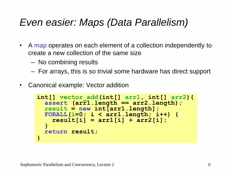
Even easier: Maps (Data Parallelism)

• A map operates on each element of a collection independently to

create a new collection of the same size

– No combining results

– For arrays, this is so trivial some hardware has direct support

• Canonical example: Vector addition


int[] vector_add(int[] arr1, int[] arr2){ assert (arr1.length == arr2.length); result = new int[arr1.length]; FORALL(i=0; i < arr1.length; i++) { result[i] = arr1[i] + arr2[i]; } return result; }

Maps in ForkJoin Framework

• Even though there is no result-combining, it still helps with load

balancing to create many small tasks

– Maybe not for vector-add but for more compute-intensive maps

– The forking is O(log n) whereas theoretically other approaches

to vector-add is O(1)


class VecAdd extends RecursiveAction { int lo; int hi; int[] res; int[] arr1; int[] arr2; VecAdd(int l,int h,int[] r,int[] a1,int[] a2){ … } protected void compute(){ if(hi – lo < SEQUENTIAL_CUTOFF) { for(int i=lo; i < hi; i++) res[i] = arr1[i] + arr2[i]; } else { int mid = (hi+lo)/2; VecAdd left = new VecAdd(lo,mid,res,arr1,arr2); VecAdd right= new VecAdd(mid,hi,res,arr1,arr2); left.fork(); right.compute(); left.join(); } } } int[] add(int[] arr1, int[] arr2){ assert (arr1.length == arr2.length); int[] ans = new int[arr1.length]; ForkJoinPool.commonPool().invoke //needs Java 8+ (new VecAdd(0,arr.length,ans,arr1,arr2); return ans; }

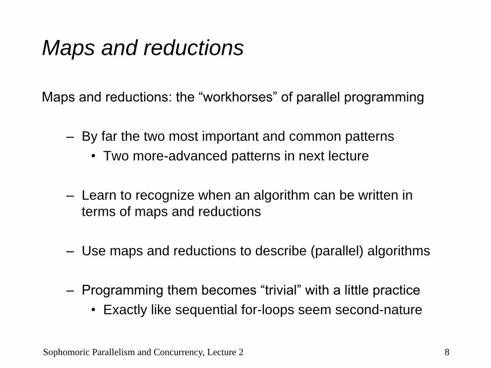
Maps and reductions

Maps and reductions: the “workhorses” of parallel programming

– By far the two most important and common patterns

• Two more-advanced patterns in next lecture

– Learn to recognize when an algorithm can be written in

terms of maps and reductions

– Use maps and reductions to describe (parallel) algorithms

– Programming them becomes “trivial” with a little practice

• Exactly like sequential for-loops seem second-nature


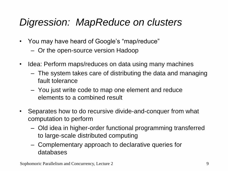
Digression: MapReduce on clusters

• You may have heard of Google’s “map/reduce”

– Or the open-source version Hadoop

• Idea: Perform maps/reduces on data using many machines

– The system takes care of distributing the data and managing

fault tolerance

– You just write code to map one element and reduce

elements to a combined result

• Separates how to do recursive divide-and-conquer from what

computation to perform

– Old idea in higher-order functional programming transferred

to large-scale distributed computing

– Complementary approach to declarative queries for

databases


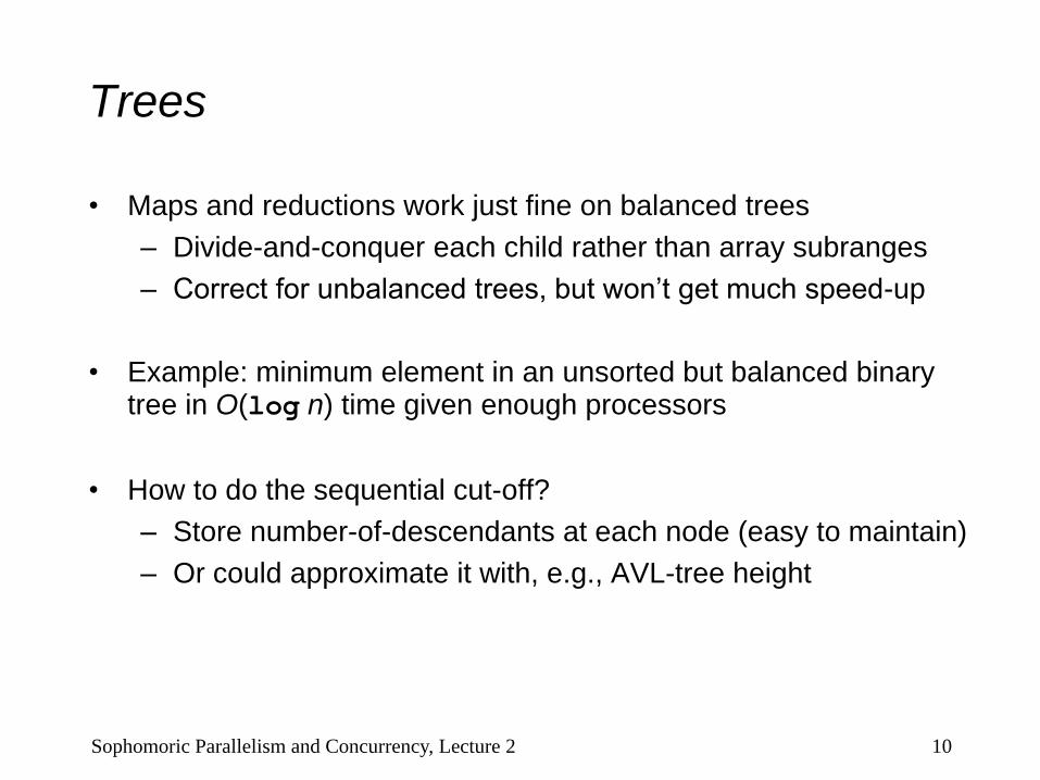
Trees

• Maps and reductions work just fine on balanced trees

– Divide-and-conquer each child rather than array subranges

– Correct for unbalanced trees, but won’t get much speed-up

• Example: minimum element in an unsorted but balanced binary tree in O(log n) time given enough processors

• How to do the sequential cut-off?

– Store number-of-descendants at each node (easy to maintain)

– Or could approximate it with, e.g., AVL-tree height


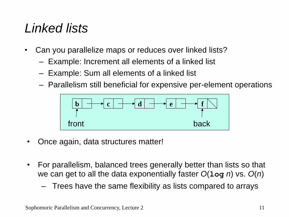
Linked lists

• Can you parallelize maps or reduces over linked lists?

– Example: Increment all elements of a linked list

– Example: Sum all elements of a linked list

– Parallelism still beneficial for expensive per-element operations


b c d e f

front back

• Once again, data structures matter!

• For parallelism, balanced trees generally better than lists so that we can get to all the data exponentially faster O(log n) vs. O(n)

– Trees have the same flexibility as lists compared to arrays

Analyzing algorithms

• Like all algorithms, parallel algorithms should be:

– Correct

– Efficient

• For our algorithms so far, correctness is “obvious” so we’ll focus

on efficiency

– Want asymptotic bounds

– Want to analyze the algorithm without regard to a specific

number of processors

– The key “magic” of the ForkJoin Framework is getting

expected run-time performance asymptotically optimal for the

available number of processors

• So we can analyze algorithms assuming this guarantee


Work and Span

Let TP be the running time if there are P processors available

Two key measures of run-time:

• Work: How long it would take 1 processor = T1

– Just “sequentialize” the recursive forking

• Span: How long it would take infinity processors = T – The longest dependence-chain

– Example: O(log n) for summing an array

• Notice having > n/2 processors is no additional help

– Also called “critical path length” or “computational depth”


The DAG

• A program execution using fork and join can be seen as a DAG

– Nodes: Pieces of work

– Edges: Source must finish before destination starts


• A fork “ends a node” and makes

two outgoing edges

• New thread

• Continuation of current thread

• A join “ends a node” and makes

a node with two incoming edges

• Node just ended

• Last node of thread joined on

Our simple examples

• fork and join are very flexible, but divide-and-conquer maps

and reductions use them in a very basic way:

– A tree on top of an upside-down tree


base cases

divide

combine

results

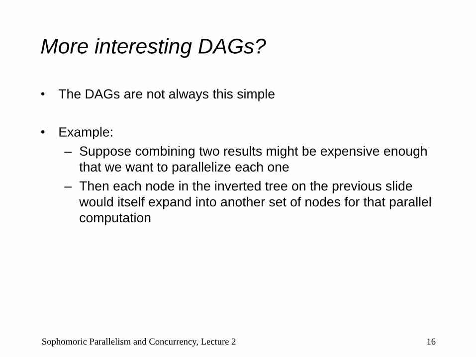
More interesting DAGs?

• The DAGs are not always this simple

• Example:

– Suppose combining two results might be expensive enough

that we want to parallelize each one

– Then each node in the inverted tree on the previous slide

would itself expand into another set of nodes for that parallel

computation


Connecting to performance

• Recall: TP = running time if there are P processors available

• Work = T1 = sum of run-time of all nodes in the DAG

– That lonely processor does everything

– Any topological sort is a legal execution

– O(n) for simple maps and reductions

• Span = T = sum of run-time of all nodes on the most-expensive

path in the DAG

– Note: costs are on the nodes not the edges

– Our infinite army can do everything that is ready to be done,

but still has to wait for earlier results

– O(log n) for simple maps and reductions


Definitions

A couple more terms:

• Speed-up on P processors: T1 / TP

• If speed-up is P as we vary P, we call it perfect linear speed-up

– Perfect linear speed-up means doubling P halves running time

– Usually our goal; hard to get in practice

• Parallelism is the maximum possible speed-up: T1 / T

– At some point, adding processors won’t help

– What that point is depends on the span

Parallel algorithms is about decreasing span without

increasing work too much


Optimal TP: Thanks ForkJoin library!

• So we know T1 and T but we want TP (e.g., P=4)

• Ignoring memory-hierarchy issues (caching), TP can’t beat

– T1 / P why not?

– T why not?

• So an asymptotically optimal execution would be:

TP = O((T1 / P) + T )

– First term dominates for small P, second for large P

• The ForkJoin Framework gives an expected-time guarantee of

asymptotically optimal!

– Expected time because it flips coins when scheduling

– How? For an advanced course (few need to know)

– Guarantee requires a few assumptions about your code…


Division of responsibility

• Our job as ForkJoin Framework users:

– Pick a good algorithm, write a program

– When run, program creates a DAG of things to do

– Make all the nodes a small-ish and approximately equal

amount of work

• The framework-writer’s job:

– Assign work to available processors to avoid idling

• Let framework-user ignore all scheduling issues

– Keep constant factors low

– Give the expected-time optimal guarantee assuming

framework-user did his/her job

TP = O((T1 / P) + T )


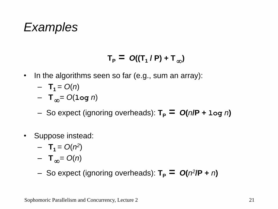
Examples

TP = O((T1 / P) + T )

• In the algorithms seen so far (e.g., sum an array):

– T1 = O(n)

– T = O(log n)

– So expect (ignoring overheads): TP = O(n/P + log n)

• Suppose instead:

– T1 = O(n2)

– T = O(n)

– So expect (ignoring overheads): TP = O(n2/P + n)


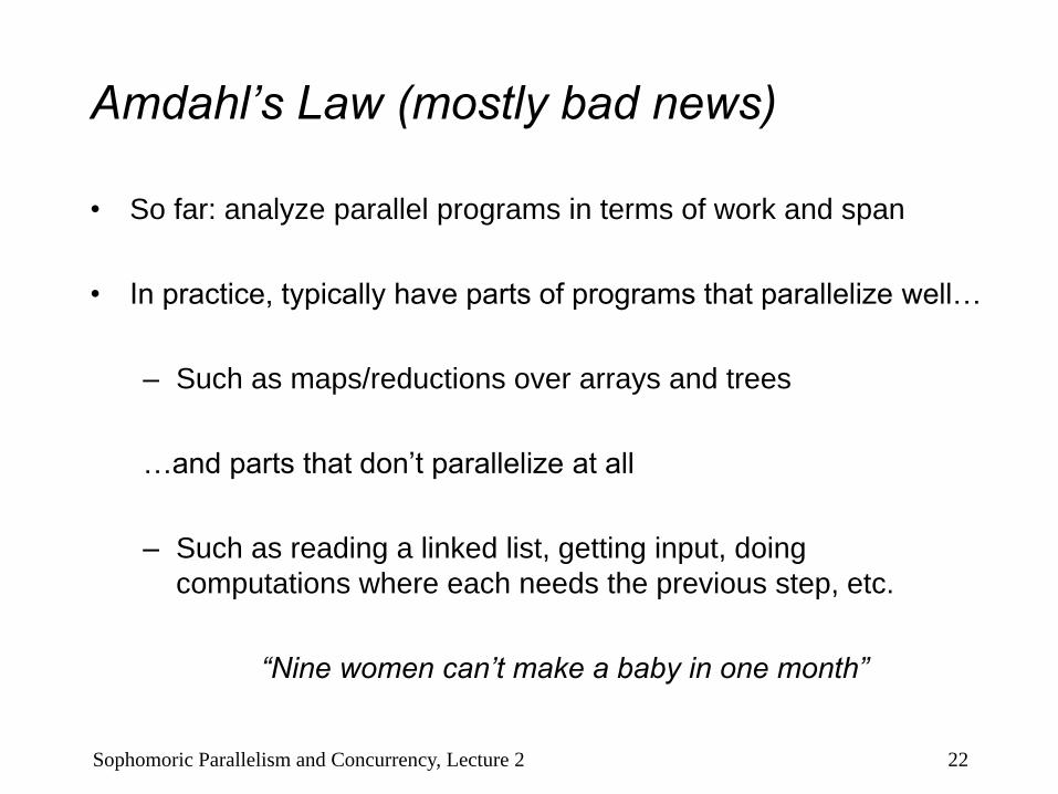
Amdahl’s Law (mostly bad news)

• So far: analyze parallel programs in terms of work and span

• In practice, typically have parts of programs that parallelize well…

– Such as maps/reductions over arrays and trees

…and parts that don’t parallelize at all

– Such as reading a linked list, getting input, doing

computations where each needs the previous step, etc.

“Nine women can’t make a baby in one month”


Amdahl’s Law (mostly bad news)

Let the work (time to run on 1 processor) be 1 unit time

Let S be the portion of the execution that can’t be parallelized

Then: T1 = S + (1-S) = 1

Suppose we get perfect linear speedup on the parallel portion

Then: TP = S + (1-S)/P

So the overall speedup with P processors is (Amdahl’s Law):

T1 / TP = 1 / (S + (1-S)/P)

And the parallelism (infinite processors) is:

T1 / T = 1 / S


Why such bad news

T1 / TP = 1 / (S + (1-S)/P) T1 / T = 1 / S

• Suppose 33% of a program’s execution is sequential

– Then a billion processors won’t give a speedup over 3

• Suppose you miss the good old days (1980-2005) where 12ish

years was long enough to get 100x speedup

– Now suppose in 12 years, clock speed is the same but you

get 256 processors instead of 1

– For 256 processors to get at least 100x speedup, we need

100 1 / (S + (1-S)/256)

Which means S .0061 (i.e., 99.4% perfectly parallelizable)


Plots you have to see

1. Assume 256 processors

– x-axis: sequential portion S, ranging from .01 to .25

– y-axis: speedup T1 / TP (will go down as S increases)

2. Assume S = .01 or .1 or .25 (three separate lines)

– x-axis: number of processors P, ranging from 2 to 32

– y-axis: speedup T1 / TP (will go up as P increases)

Do this as a homework problem!

– Chance to use a spreadsheet or other graphing program

– Compare against your intuition

– A picture is worth 1000 words, especially if you made it


All is not lost

Amdahl’s Law is a bummer!

– Unparallelized parts become a bottleneck very quickly

– But it doesn’t mean additional processors are worthless

• We can find new parallel algorithms

– Some things that seem sequential are actually parallelizable

• We can change the problem or do new things

– Example: Video games use tons of parallel processors

• They are not rendering 10-year-old graphics faster

• They are rendering more beautiful(?) monsters


Moore and Amdahl

• Moore’s “Law” is an observation about the progress of the

semiconductor industry

– Transistor density doubles roughly every 18 months

• Amdahl’s Law is a mathematical theorem

– Diminishing returns of adding more processors

• Both are incredibly important in designing computer systems


Documents

A Sophomoric Introduction to Shared-Memory Parallelism and ...homes.cs.washington.edu/~djg/teachingMaterials/... · – Combines results in parallel • Some Java and ForkJoin Framework