A SON-Based Algorithm for the Optimization of Inter-RAT ...kang.nt.e-technik.tu-darmstadt.de/nt/fileadmin/kt/Publikationen... · 1906 IEEETRANSACTIONS ON VEHICULAR TECHNOLOGY, VOL.62,NO.5,JUNE

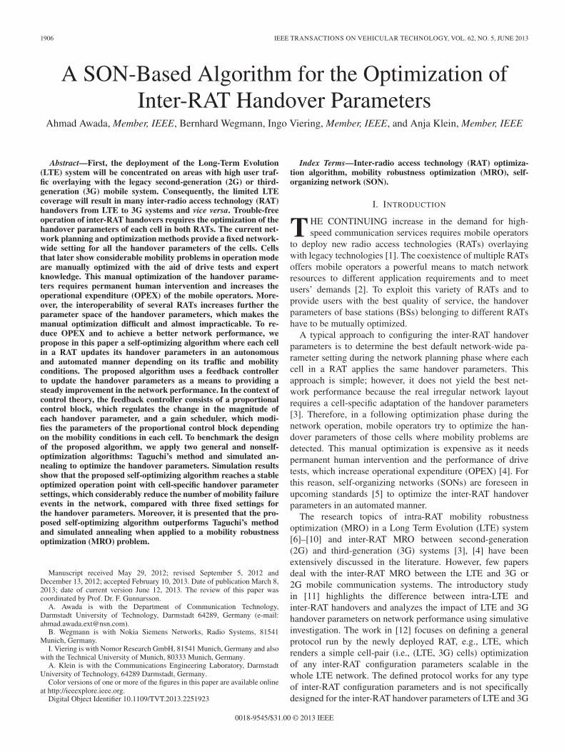
1906 IEEE TRANSACTIONS ON VEHICULAR TECHNOLOGY, VOL. 62, NO. 5, JUNE 2013

A SON-Based Algorithm for the Optimization ofInter-RAT Handover Parameters

Ahmad Awada, Member, IEEE, Bernhard Wegmann, Ingo Viering, Member, IEEE, and Anja Klein, Member, IEEE

Abstract—First, the deployment of the Long-Term Evolution(LTE) system will be concentrated on areas with high user traf-fic overlaying with the legacy second-generation (2G) or third-generation (3G) mobile system. Consequently, the limited LTEcoverage will result in many inter-radio access technology (RAT)handovers from LTE to 3G systems and vice versa. Trouble-freeoperation of inter-RAT handovers requires the optimization of thehandover parameters of each cell in both RATs. The current net-work planning and optimization methods provide a fixed network-wide setting for all the handover parameters of the cells. Cellsthat later show considerable mobility problems in operation modeare manually optimized with the aid of drive tests and expertknowledge. This manual optimization of the handover parame-ters requires permanent human intervention and increases theoperational expenditure (OPEX) of the mobile operators. More-over, the interoperability of several RATs increases further theparameter space of the handover parameters, which makes themanual optimization difficult and almost impracticable. To re-duce OPEX and to achieve a better network performance, wepropose in this paper a self-optimizing algorithm where each cellin a RAT updates its handover parameters in an autonomousand automated manner depending on its traffic and mobilityconditions. The proposed algorithm uses a feedback controllerto update the handover parameters as a means to providing asteady improvement in the network performance. In the context ofcontrol theory, the feedback controller consists of a proportionalcontrol block, which regulates the change in the magnitude ofeach handover parameter, and a gain scheduler, which modi-fies the parameters of the proportional control block dependingon the mobility conditions in each cell. To benchmark the designof the proposed algorithm, we apply two general and nonself-optimization algorithms: Taguchi’s method and simulated an-nealing to optimize the handover parameters. Simulation resultsshow that the proposed self-optimizing algorithm reaches a stableoptimized operation point with cell-specific handover parametersettings, which considerably reduce the number of mobility failureevents in the network, compared with three fixed settings forthe handover parameters. Moreover, it is presented that the pro-posed self-optimizing algorithm outperforms Taguchi’s methodand simulated annealing when applied to a mobility robustnessoptimization (MRO) problem.

Manuscript received May 29, 2012; revised September 5, 2012 andDecember 13, 2012; accepted February 10, 2013. Date of publication March 8,2013; date of current version June 12, 2013. The review of this paper wascoordinated by Prof. Dr. F. Gunnarsson.

A. Awada is with the Department of Communication Technology,Darmstadt University of Technology, Darmstadt 64289, Germany (e-mail:[email protected]).

B. Wegmann is with Nokia Siemens Networks, Radio Systems, 81541Munich, Germany.

I. Viering is with Nomor Research GmbH, 81541 Munich, Germany and alsowith the Technical University of Munich, 80333 Munich, Germany.

A. Klein is with the Communications Engineering Laboratory, DarmstadtUniversity of Technology, 64289 Darmstadt, Germany.

Color versions of one or more of the figures in this paper are available onlineat http://ieeexplore.ieee.org.

Digital Object Identifier 10.1109/TVT.2013.2251923

Index Terms—Inter-radio access technology (RAT) optimiza-tion algorithm, mobility robustness optimization (MRO), self-organizing network (SON).

I. INTRODUCTION

THE CONTINUING increase in the demand for high-speed communication services requires mobile operators

to deploy new radio access technologies (RATs) overlayingwith legacy technologies [1]. The coexistence of multiple RATsoffers mobile operators a powerful means to match networkresources to different application requirements and to meetusers’ demands [2]. To exploit this variety of RATs and toprovide users with the best quality of service, the handoverparameters of base stations (BSs) belonging to different RATshave to be mutually optimized.

A typical approach to configuring the inter-RAT handoverparameters is to determine the best default network-wide pa-rameter setting during the network planning phase where eachcell in a RAT applies the same handover parameters. Thisapproach is simple; however, it does not yield the best net-work performance because the real irregular network layoutrequires a cell-specific adaptation of the handover parameters[3]. Therefore, in a following optimization phase during thenetwork operation, mobile operators try to optimize the han-dover parameters of those cells where mobility problems aredetected. This manual optimization is expensive as it needspermanent human intervention and the performance of drivetests, which increase operational expenditure (OPEX) [4]. Forthis reason, self-organizing networks (SONs) are foreseen inupcoming standards [5] to optimize the inter-RAT handoverparameters in an automated manner.

The research topics of intra-RAT mobility robustnessoptimization (MRO) in a Long Term Evolution (LTE) system[6]–[10] and inter-RAT MRO between second-generation(2G) and third-generation (3G) systems [3], [4] have beenextensively discussed in the literature. However, few papersdeal with the inter-RAT MRO between the LTE and 3G or2G mobile communication systems. The introductory studyin [11] highlights the difference between intra-LTE andinter-RAT handovers and analyzes the impact of LTE and 3Ghandover parameters on network performance using simulativeinvestigation. The work in [12] focuses on defining a generalprotocol run by the newly deployed RAT, e.g., LTE, whichrenders a simple cell-pair (i.e., (LTE, 3G) cells) optimizationof any inter-RAT configuration parameters scalable in thewhole LTE network. The defined protocol works for any typeof inter-RAT configuration parameters and is not specificallydesigned for the inter-RAT handover parameters of LTE and 3G

0018-9545/$31.00 © 2013 IEEE

AWADA et al.: SON-BASED ALGORITHM FOR OPTIMIZATION OF INTER-RAT HANDOVER PARAMETERS 1907

systems. Moreover, the latter work does not specify or describethe algorithm needed for optimizing the inter-RAT handoverparameters of LTE and 3G systems in a cell-pair manner.

In this paper, we propose a new SON-based algorithm forthe optimization of inter-RAT handover parameters of LTE and3G systems. The algorithm is run by each cell in both RATsin an autonomous and automated way. Each cell updates itshandover parameters based on the values of predefined keyperformance indicators (KPIs), which capture the number andthe type of mobility failure events in each cell. The changesin the magnitude of the handover parameters of each cell aredetermined by a feedback controller [13]. In the vocabularyof control theory, the two main components of the feedbackcontroller are the proportional control block [13] and thegain scheduler [14], [15]. The change in the magnitude ofeach handover parameter is determined by the first controlblock and is proportional to a predefined error signal. Thegain scheduler alters the behavior of the proportional controlblock by modifying its parameters [14], [15] depending onthe mobility conditions in each cell. In addition to the newproposed self-optimizing algorithm, we apply two other well-known optimization methods: Taguchi’s method [16] and sim-ulated annealing [17] to optimize the inter-RAT handoversparameters of LTE and 3G systems. Simulated annealing is anoptimization method that has been extensively used in manyengineering problems [18], [19]. Taguchi’s method is anotherpromising optimization method that was first developed forthe optimization of manufacturing processes [20] and has beenrecently introduced to wireless mobile communication field in[21]–[25]. Taguchi’s method and simulated annealing cannotbe used as self-optimizing algorithms because they need toperform network trials, i.e., test handover parameter settings,which is not possible in a real-time network. However, thesetwo optimization methods are used in our context to benchmarkthe design of our proposed self-optimizing algorithm.

This paper is organized as follows. In Section II, the inter-RAT handover procedure comprising the handover-related pa-rameters and the measurements leading to handover decisionsare explained. The inter-RAT KPIs and their root-cause analysisare discussed in Section III. An overall description of the pro-posed self-optimizing algorithm for the inter-RAT LTE and 3Ghandover parameters is presented in Section IV. In Section V,we focus on describing in detail the two components of thefeedback controller: the proportional control block and the gainscheduler. The simulation scenario and parameters for the LTEand 3G downlink systems are described in Section VI. Simu-lation results are shown in Section VII, and the performanceof the proposed inter-RAT MRO algorithm is compared withthose of three fixed handover parameter settings. In addition,the performance of the proposed algorithm is compared withthose achieved by Taguchi’s method and simulated annealing.This paper is then concluded in Section VIII.

II. INTER-RADIO ACCESS TECHNOLOGY

HANDOVER PROCEDURE

Here, the inter-RAT handover measurements and parametersare explained after giving a few definitions.

A. General Definitions

• The RAT to which a cell c in LTE or 3G belongs isdetermined by the function r = R(c), where r is eitherequal to LTE or 3G.

• Cell c serving user equipment (UE) u at time instant t isgiven by connection function c = xu(t).

• The downlink signal-to-interference-plus-noise ratio(SINR) of UE u served by cell c at time instant t isdenoted by γu, c(t).

• A radio link failure (RLF) is detected at time instant t0 ifthe SINR of UE u falls below a certain threshold Qout fora certain time interval TQout

, i.e.,

γu, c(t) < Qout for t0 − TQout< t < t0. (1)

B. Inter-RAT Handover Measurements and Parameters

The serving BS in LTE or 3G networks configures the UE toperform signal strength measurements for the serving and intra-or inter-RAT neighboring cells. The criteria for the UE to sendits measurements in a report to the serving BS can be either pe-riodic or event triggered. For an event triggered report, the UEsends its measurement report when a certain condition, whichis called the entering condition of the measurement event, isfulfilled for a time-to-trigger (TTT) time interval denoted byTT . The parameters of the entering condition of a measurementevent are configured by the serving BS. The handover of theUE is triggered by the serving BS when a measurement reportis received.

To hand over the UE from LTE to 3G, the serving BS inLTE configures the UE with measurement event B2 [26]. Asimilar measurement event exists for handing over the UE ina 3G cell to another LTE cell, which is called event 3A [27].Both measurement events B2 and 3A require the UE to measurethe received signal strength of both the serving and handovertarget cells. For an LTE cell, the UE measures the referencesignal received power (RSRP), which is defined as the linearaverage over the power contributions of the resource elementsthat carry cell-specific reference signals within the consideredmeasured frequency bandwidth [28]. In the case of a 3G cell,the UE measures the received signal code power (RSCP), whichis defined as the received power on one code measured on theprimary common pilot channel (CPICH) [28]. Both RSRP andRSCP include path loss, antenna gain, lognormal shadowing,and fast fading.

The received signal strength of serving cell c measured byUE u is expressed as a function of time t by Su, c(t) in dBm, i.e.,Su, c(t) is equivalent to RSRP or RSCP if the UE is connectedto LTE or 3G, respectively. Similarly, the signal strength of thehandover target cell c0 of UE u is expressed by Tu, c0(t) indBm. Target cell c0 is defined as the neighboring inter-RATcell corresponding to the strongest signal strength measuredand reported by UE u. The entering condition of measurementevent B2 or 3A is fulfilled when the signal of the serving cellSu, c(t) falls below a first threshold Sthr expressed in dBm, andthe signal of the target cell Tu, c0(t) is higher than a secondthreshold Tthr in dBm. The UE sends the measurement report at


time instant t0 when the entering condition of the measurementevent is fulfilled for a time interval of TT duration, i.e.,

Su, c(t) < Sthr ∧ Tu, c0(t) > Tthr for t0 − TT < t < t0such that R(c) �= R(c0). (2)

In principle, the UE starts to measure the neighboring inter-RAT cells when the signal strength of the serving cell fallsbelow a certain network-configured threshold. The latter thresh-old would be set slightly above Sthr, so that Tu, c0(t) wouldbe available when the UE checks if the entering condition ofthe measurement event is fulfilled. In this paper, we assumefor simplicity that the inter-RAT measurements are alwaysavailable for the UE. It is also worth noting that, to measurethe signal strength of neighboring inter-RAT cells, the UEhas to interrupt its serving connection for measurement gaps[29]. From that perspective, inter-RAT measurements are quitecostly, unlike the intra-RAT case, which does not require anymeasurement gaps.

The two thresholds Sthr and Tthr are called inter-RAT han-dover thresholds, and these shall be optimized by the inter-RAT MRO algorithm, assuming that TT is configured properly.Large TT values can avoid handovers caused by measurementoutliers; however, they may delay the handover decisions thatmay lead to RLFs, particularly for fast UEs. Extending the inter-RAT MRO algorithm to comprise TT optimization is left forfuture work.

C. Execution of the Inter-RAT Handover

After a measurement report is sent by UE u, serving cellc prepares the handover of the UE by sending a handoverrequest to target handover cell c0. Then, serving cell c waitsfor an acknowledgment from target cell c0. This step inducesan additional delay THP, which we typically call handoverpreparation time. Therefore, the handover of UE u is executedTHP s after the measurement event is triggered as long as theSINR γu, c(t) of the UE is greater than threshold Qfail. In otherwords, the handover of UE u is executed from cell c to cell c0at time instant tHO if the following conditions hold:

xu(t) = c0 for t > tHO

if Su, c(t) < Sthr ∧ Tu, c0(t) > Tthr

for tHO − THP − TT < t < tHO − THP,

R(c) �= R(c0), and γu, c(tHO) > Qfail. (3)

Connection function xu(t) is changed to c0 at time instance tHO

until the succeeding handover is executed.

III. KPIs FOR INTER-RADIO ACCESS TECHNOLOGY

MOBILITY PERFORMANCE

Here, the inter-RAT mobility KPIs and the root-cause anal-ysis of each type of mobility failure events are presented. Themore detailed the information about the mobility failure events,the better the optimization algorithm is. In accordance withthe mobility failure types defined for the intra-LTE case [5],two categories are specified here for the inter-RAT scenario:

The first category captures inter-RAT RLFs and the secondcagetory captures the costly inter-RAT handovers, such as ping-pongs (PPs), which refer to events where the UE is immediatelyhanded back over to a cell of its previous RAT after a successfulinter-RAT handover.

A. Inter-RAT RLF KPIs

There are three types of RLF mobility events: 1) a too-lateinter-RAT handover (TLH); 2) a too-early inter-RAT handover(TEH); and 3) an inter-RAT handover to a wrong cell (HWC).

1) TLH: The UE drops before a handover is initiated or exe-cuted from one RAT to another, and the UE reconnects to a cellin a RAT, which is different than that of the previously servingcell. The reason for a TLH is either the entering condition ofthe measurement event had not been fulfilled or the enteringcondition of the measurement event had been fulfilled, but theRLF occurred before the inter-RAT handover is executed.

The entering condition of a measurement event is not fulfilledin three different cases.

• Case A: Su, c(t) is below Sthr and Tu, c0(t) is below Tthr

[see Fig. 1(a)].• Case B: Su, c(t) is higher than Sthr and Tu, c0(t) is higher

than Tthr [see Fig. 1(b)].• Case C: Su, c(t) is higher than Sthr and Tu, c0(t) is below

Tthr [see Fig. 1(c)].In another case, denoted as Case D and shown in Fig. 1(d),

the entering condition of the measurement event is fulfilled, butnevertheless, the RLF occurred before the inter-RAT handoveris completed.

In an intra-RAT case, a single handover threshold is used,and consequently, one type of TLH exists. However, in an inter-RAT case, there are two thresholds controlling each measure-ment event B2 and 3A, and the root cause for a TLH is themisconfiguration of either Sthr or Tthr. A TLH due to themisconfiguration of Sthr or Tthr is denoted by TLH(Sthr) orTLH(Tthr), respectively. Our proposal to distinguish betweenthe two types TLH(Sthr) and TLH(Tthr) has been recentlyadopted by LTE Release 11 (Rel. 11) standard [30], [31]. InCase A, the entering condition of the measurement event is notfulfilled because Tthr is set to a too high value, which cannotbe achieved, i.e., the RLF occurred before Tu, c0(t) becomeshigher than Tthr. In this case, the misconfiguration of Tthr isthe root cause for the TLH. Similarly, in Case B, the enteringcondition of the measurement event is not fulfilled because Sthr

is set to a too low value, and the RLF occurred before Su, c(t)becomes lower than Sthr. In this case, the misconfiguration ofSthr is the root cause for the TLH.

For Cases C and D, the root cause for the TLH is not asobvious as in Cases A and B. In Case C, none of the twothresholds is reached, i.e., Su, c(t) > Sthr and Tu, c0(t) < Tthr,and in Case D, both thresholds are reached, i.e., Su, c(t) < Sthr

and Tu, c0(t) > Tthr. In Case C, the root cause for the TLHis, in principle, the misconfiguration of both Sthr and Tthr

thresholds because they are not reached. However, as each TLHshould be counted as a single mobility failure event, it hasto be classified as either TLH(Sthr) or TLH(Tthr). For thispurpose, we propose a new classification rule that is based


Fig. 1. Four different cases for inter-RAT TLH. (a) Case A where the entering condition of the measurement event is not fulfilled. The misconfiguration ofTthr is the root cause for the TLH. (b) Case B where the entering condition of the measurement event is not fulfilled. The misconfiguration of Sthr is the rootcause for the TLH. (c) Case C where the entering condition of the measurement event is not fulfilled. The misconfiguration of the threshold corresponding to thesmallest value between ΔS and ΔT is identified as the root cause for the TLH. (d) Case D where the entering condition of the measurement event is fulfilled. Themisconfiguration of one of the two thresholds, which is reached later, is identified as the root cause for the TLH.

on the differences between the values of the thresholds andtheir corresponding measured signal levels evaluated at tRLF.Let ΔS = Sthr − Su, c(tRLF) and ΔT = Tu, c0(tRLF)− Tthr

be the differences corresponding to thresholds Sthr and Tthr,respectively. The root cause for the TLH in Case C is identifiedas the misconfiguration of the threshold of which the differenceis the smallest. The rule determines the threshold that has tobe adjusted first by comparing the two negative values ΔS

and ΔT . Once the threshold corresponding to the smallestdifference is correctly adjusted in subsequent steps, i.e., itscorresponding value of ΔS or ΔT becomes positive, the ruledetects that the other threshold having ΔS < 0 or ΔT < 0 hasto be adjusted. As a result, the rule needs multiple steps todetect that both thresholds have to be adjusted and consequentlyresolve the TLH. The proposed routine for classifying a TLHas either TLH(Sthr) or TLH(Tthr) in Cases A, B, and C issummarized in pseudocode 1.

Pseudocode 1: Routine for classifying a TLH as eitherTLH(Sthr) or TLH(Tthr).

1: Input Parameters: Su, c(tRLF), Tu, c0(tRLF), Sthr,and Tthr.

2: Calculate ΔS = Sthr − Su, c(tRLF).3: Calculate ΔT = Tu, c0(tRLF)− Tthr.4: if ΔS < ΔT

5: TLH is classified as TLH(Sthr).6: else

7: TLH is classified as TLH(Tthr).8: end if

As for Case D, the root cause for the TLH cannot bedetermined using the aforementioned pseudocode. In this case,the root cause for the TLH is the misconfiguration of oneof the two thresholds, which is reached later. For clarity, anexample is shown in Fig. 1(d), which shows Case D. Accordingto the figure, the entering condition of the measurement eventis fulfilled; nevertheless, an RLF occured before the TT timeinterval is completed. The TLH could be resolved if the enteringcondition would have been fulfilled earlier. To this end, thethreshold that delayed the fulfillment of the entering conditionneeds to be determined and adjusted. In this example, Tthr isreached before Sthr, and the root cause for this RLF is themisconfiguration of Sthr. Decreasing Tthr would not solve theTLH as the entering condition would not be fulfilled earliersince Su, c(t) is greater than Sthr. However, if Sthr is reachedearlier, the entering condition of the measurement event wouldhave been fulfilled earlier, and the RLF would have beenavoided. We note that to resolve TLH(Sthr), Sthr should beincreased, whereas TLH(Tthr) is resolved by decreasing theTthr threshold.

2) TEH: The UE is successfully handed over from cell Ato another cell B of a different RAT. Shortly after, an RLFhappens, and the UE reconnects to the previous RAT, either tothe same cell A or to a different one. Moreover, the inter-RAThandover failure, occurring when the UE fails during the


handover to connect to the target handover cell c0 using therandom access channel [32], is also considered a TEH. The rootcause for a TEH is the misconfiguration of Tthr, which shouldbe increased to guarantee that the signal of the target cell of adifferent RAT is strong enough.

3) HWC: The UE is successfully handed over from cell Ato another cell B of a different RAT. Shortly after, an RLFhappens, and the UE reconnects to a third cell C belongingto the same RAT as cell B. Similar to a TEH, the root causefor a HWC is the misconfiguration of Tthr, which should beincreased to guarantee that the signal of a cell of a differentRAT is strong enough.

B. Costly Inter-RAT Handovers

There are two types of costly inter-RAT handovers: Inter-RAT PPs and unnecessary handovers (UHs) from LTE to 3G.The number of UHs has to be minimized as the users shouldbenefit as much as possible from the newly deployed LTEnetwork, which is given, in our case, a higher priority than 3G.

1) PP: The UE is handed over to a cell of a different RAT,and within time interval TPP, the UE is handed over back to thesame cell or to a different cell of the previous RAT. The actionneeded to resolve a PP is to delay the first inter-RAT handoverby either decreasing Sthr or increasing Tthr.

2) UH: The UE is handed over from a high-priority RAT(LTE in our case) to a low priority RAT (3G), although thesignal quality of the previous LTE cell is still good enough[32]. In this paper, an inter-RAT handover is detected as un-necessary if, after the handover, the reference signal receivedquality (RSRQ) of the previous LTE cell is still higher thanthreshold QRSRQ for time interval TQRSRQ

. The action neededto resolve UHs is to increase the coverage of the LTE cell bydecreasing Sthr.

In this paper, we consider all types of mobility failuresand costly handovers for the inter-RAT scenario. However, inpractice, the Third-Generation Partnership Project has focusedonly on a subset of the aforementioned KPIs. The LTE Rel.10 standard has specified the detection of UHs, whereas LTERel. 11 has recently considered TLHs from LTE to 3G, TEHsfrom 3G to LTE, and PPs in both RATs [32].

IV. DESCRIPTION OF THE SELF-OPTIMIZING ALGORITHM

FOR INTER-RADIO ACCESS TECHNOLOGY

HANDOVER-RELATED PARAMETERS

Here, we give a general overview of the proposed inter-RAT MRO algorithm. Some of the inter-RAT KPIs definedin Section III require the same action to be performed on thevalue of a handover threshold, i.e., either increase or decrease.Therefore, we group the values of the inter-RAT KPIs into newother values depending on the action that needs to be applied oneach handover threshold. The feedback controller determinesthe change in the magnitude of each handover threshold basedon the aforementioned new values.

A. Grouping the Values of the Inter-RAT KPIs

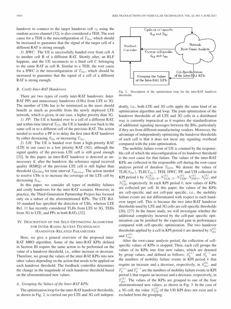
The optimization loop for the inter-RAT handover thresholds,as shown in Fig. 2, is carried out per LTE and 3G cell indepen-

Fig. 2. Description of the optimization loop for the inter-RAT handoverthresholds.

dently, i.e., both LTE and 3G cells apply the same kind of anoptimization algorithm and loop. The joint optimization of thehandover thresholds of all LTE and 3G cells in a distributedway is currently impractical as it requires the standardizationof additional signaling messages between the BSs, particularlyif they are from different manufacturing vendors. Moreover, theadvantage of independently optimizing the handover thresholdsof each cell is that it does not incur any signaling overheadcompared with the joint optimization.

The mobility failure event of UE is counted by the responsi-ble cell of which the misconfiguration of its handover thresholdis the root cause for that failure. The values of the inter-RATKPIs are collected in the responsible cell during the root-causeanalysis period of duration TKPI. We denote the values ofTLH(Sthr), TLH(Tthr), TEH, HWC, PP, and UH collected inKPI period k by N

(k)TLH−S, N (k)

TLH−T, N (k)TEH, N (k)

HWC, N (k)PP , and

N(k)UH, respectively. In each KPI period k, new values of KPIs

are collected per cell. In this paper, the values of the KPIsare cell-specific and not cell-pair specific, i.e., the mobilityfailure events are not differentiated with respect to each hand-over target cell. This is because the two inter-RAT handoverthresholds used by LTE and 3G cells are cell-specific thresholds[26], [27]. In the future study, we will investigate whether theadditional complexity incurred by the cell-pair specific opti-mization can be justified by the expected gain in performancecompared with cell-specific optimization. The two handoverthresholds applied by a cell in KPI period k are denoted by S

(k)thr

and T(k)thr .

After the root-cause analysis period, the collection of cell-specific values of KPIs is stopped. Then, each cell groups thevalues of its KPIs into four new values, which are denotedby group values, and defined as follows: S

(+)k and S

(−)k are

the numbers of mobility failure events in KPI period k thatrequire an increase and a decrease, respectively, in S

(k)thr , and

T(+)k and T

(−)k are the numbers of mobility failure events in KPI

period k that require an increase and a decrease, respectively, inT

(k)thr . The values of the KPIs are grouped to one of the four

aforementioned new values, as shown in Fig. 3. In the case ofa 3G cell, the value N

(k)UH of the UH KPI does not exist and is

excluded from the grouping.


Fig. 3. Grouping the values of the KPIs into four new values based on theactions required for updating the handover thresholds. In the case of a 3G cell,

N(k)UH does not exist and is excluded.

The main aim of the inter-RAT MRO algorithm is to resolveRLFs and high N

(k)PP might prevent the algorithm from reacting

on N(k)TLH−S and N

(k)TLH−T. To overcome this problem, N (k)

PP

is weighted by coefficients ws ≤ 0.5 and wt ≤ 0.5 to give ahigher priority for RLFs. In this case, each PP event is counted(ws + wt) ≤ 1 times compared with an RLF event, which iscounted once. For instance, if a weight of 0.2 is used for ws andwt, a PP event is counted (ws + wt) = 0.4 times compared withan RLF event. The higher the values of ws and wt, the higherthe probability of reducing the gains in RLFs is. Moreover,among the assignments, there is one which is conditional: N (k)

UH

is assigned to S(−)k only when there is no TLHs in the cell.

The coverage of the LTE cell should be increased only if theUE could continue in the source cell without problems, asstated in the LTE standard [33]. The existence of TLHs is anindication that the UE could not stay longer in the cell andshould be handed over earlier. As a result, reacting on UHswith the presence of TLHs is risky and may worsen the mobilityperformance of the UE. Having the values of the KPIs grouped,the four aforementioned group values are used by the feedbackcontroller to update the handover thresholds S

(k)thr and T

(k)thr of

KPI period k.

B. Description of the Feedback Controller

Here, we give a general overview of the feedback controller,which is responsible for updating the handover thresholds S(k)

thr

and T(k)thr .

In KPI period k, the input variables of the controller are thefour group values S

(+)k , S(−)

k , T (+)k , and T

(−)k obtained from

grouping the values of the KPIs in addition to the values of thethresholds S

(k−1)thr and T

(k−1)thr used in KPI period k − 1 (see

Fig. 2). The changes in the magnitude of thresholds S(k)thr and

T(k)thr are denoted by u

(k)s,dB and u

(k)t,dB, which are expressed in

decibels, respectively. The role of the feedback controller is todetermine the appropriate values of u(k)

s,dB and u(k)t,dB based on

the input variables fed to the controller in each KPI period.Threshold S

(k)thr is increased or decreased by u

(k)s,dB only if one

or both group values S(+)k and S

(−)k exceed a certain limit de-

noted by S(min). Similarly, T (k)thr is updated if one or both T

(+)k

and T(−)k exceed a predefined limit denoted by T (min). The

values of S(min) and T (min) depend mainly on the duration ofthe KPI collection period and the number of handover attemptsin the cell, i.e., too-late handovers + successful handovers.Thresholds S(min) and T (min) should be set high enough, sothat the group values can be considered statistically significantand in turn avoid reacting on outliers.

The value of u(k)s,dB is determined based on the magnitude

of S(+)k and S

(−)k . Similarly, the value of u(k)

t,dB is determined

based on the magnitude of T (+)k and T

(−)k . The value of u(k)

s,dB

depends on the difference between S(+)k and S

(−)k , as shown in

Fig. 4. The same applies for u(k)t,dB. The larger the difference

between S(+)k and S

(−)k , the larger u

(k)s,dB is. If the difference

between S(+)k and S

(−)k is significant, as in Fig. 4(a), large u(k)

s,dB

is used since one specific value is dominating and can be wellreduced. However, it may happen that two similar group valuesoccur in one cell, as shown in Fig. 4(c). In this case, the mobilityfailure events require contradicting handover threshold updates.Changing the threshold in one direction could decrease one ofthe group values more than the other one is increased; however,it would be difficult to predict the correct parameter update, i.e.,increase or decrease. Moreover, the gain would be minimal ifit exists since none of the group values can be well reducedwithout a significant increase in the other group value, i.e., thegroup values would most likely start to oscillate. Reducing theoscillations in the values of the KPIs is an important aspect inself-optimizing algorithms as they directly impact the qualityperception of the users. Therefore, in this case, we either applysmall u

(k)s,dB or avoid updating the handover threshold, i.e.,

u(k)s,dB = 0.The problem shown in Fig. 4(c) can be tackled for the target

threshold using cell-pair specific handover offsets, which allowa dedicated handover threshold value to be configured withrespect to each neighboring target cell. For clarity, assume thatT

(+)k ≈ T

(−)k and the mobility failure events of T

(+)k occur

with respect to neighboring target cell c′0, which is differentthan that of T (−)

k denoted by c′′0. By means of cell-pair specifichandover thresholds, the target threshold could be increasedwith respect to c′0 and decreased with respect to c′′0, whichconsequently resolve T

(+)k and T

(−)k . This solution is currently

not possible since the inter-RAT handover thresholds arespecified as cell-specific.

V. COMPONENTS OF THE CONTROLLER

The feedback controller, highlighted in bold in Fig. 2, iscomposed of two components: a proportional control block anda gain scheduler, as shown in Fig. 5. The input variables to thefeedback controller are the four group values and the handoverthreshold values of KPI period k − 1 and the output is theupdated handover thresholds of KPI period k.

A. Proportional Control Block

1) Calculate the Error Values: We define two metrics M (k)s

and M(k)t corresponding to handover thresholds S(k)

thr and T(k)thr ,


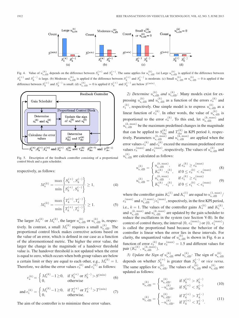
Fig. 4. Value of u(k)s,dB

depends on the difference between S(+)k

and S(−)k

. The same applies for u(k)t, dB

. (a) Large u(k)s,dB

is applied if the difference between

S(+)k

and S(−)k

is large. (b) Moderate u(k)s,dB

is applied if the difference between S(+)k

and S(−)k

is moderate. (c) Small u(k)s, dB

or u(k)s, dB

= 0 is applied if the

difference between S(+)k

and S(−)k

is small. (d) u(k)s, dB

= 0 is applied if S(+)k

and S(−)k

are below S(min).

Fig. 5. Description of the feedback controller consisting of a proportionalcontrol block and a gain scheduler.

respectively, as follows:

M (k)s =

max{S(+)k , S

(−)k

}min

{S(+)k , S

(−)k

} ≥ 1, (4)

M(k)t =

max{T

(+)k , T

(−)k

}min

{T

(+)k , T

(−)k

} ≥ 1. (5)

The larger M (k)s or M (k)

t , the larger u(k)s,dB or u(k)

t,dB is, respec-

tively. In contrast, a small M (k)s requires a small u(k)

s,dB. Theproportional control block makes corrective actions based onthe value of an error, which is defined in our case as a functionof the aforementioned metric. The higher the error value, thelarger the change in the magnitude of a handover thresholdvalue is. The handover threshold is not updated when the erroris equal to zero, which occurs when both group values are belowa certain limit or they are equal to each other, e.g., M (k)

s = 1.Therefore, we define the error values e(k)s and e

(k)t as follows:

e(k)s =

{M

(k)s −1≥0, if S(+)

k or S(−)k >S(min)

0, otherwise(6)

and e(k)t =

{M

(k)t −1≥0, if T (+)

k or T (−)k >T (min)

0, otherwise.(7)

The aim of the controller is to minimize these error values.

2) Determine u(k)s,dB and u

(k)t,dB: Many models exist for ex-

pressing u(k)s,dB and u

(k)t,dB as a function of the errors e

(k)s and

e(k)t , respectively. One simple model is to express u

(k)s,dB as a

linear function of e(k)s . In other words, the value of u

(k)s,dB is

proportional to the error e(k)s . To this end, let u

(k,max)s,dB and

u(k,max)t,dB be the maximum predefined changes in the magnitude

that can be applied to S(k)thr and T

(k)thr in KPI period k, respec-

tively. Parameters u(k,max)s,dB and u

(k,max)t,dB are applied when the

error values e(k)s and e(k)t exceed the maximum predefined error

values e(max)s and e

(max)t , respectively. The values of u(k)

s,dB and

u(k)t,dB are calculated as follows:

u(k)s,dB =

{u(k,max)s,dB , if e(k)s ≥ e

(max)s

K(k)s · e(k)s , if 0 ≤ e

(k)s < e

(max)s

(8)

u(k)t,dB =

{u(k,max)t,dB , if e(k)t ≥ e

(max)t

K(k)t · e(k)t , if 0 ≤ e

(k)t < e

(max)t

(9)

where the controller gains K(1)s and K

(1)t are equal to u

(1,max)s,dB /

e(max)s and u

(1,max)t,dB /e

(max)t , respectively, in the first KPI period,

i.e., k = 1. The values of the controller gains K(k)s and K

(k)t ,

and u(k,max)s,dB and u

(k,max)t,dB are updated by the gain scheduler to

reduce the oscillations in the system (see Section V-B). In thecontext of control theory, the interval (0, e(max)

s ) or (0, e(max)t )

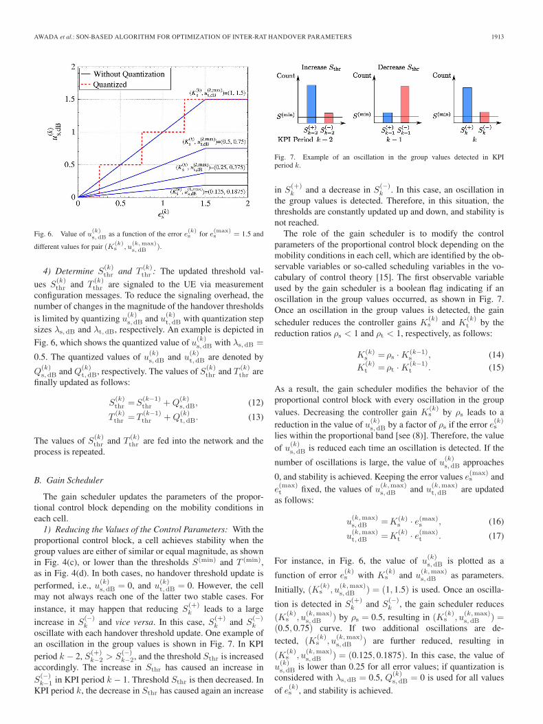
is called the proportional band because the behavior of thecontroller is linear when the error lies in these intervals. Forclarity, the unquantized value of u(k)

s,dB is shown in Fig. 6 as a

function of error e(k)s for e(max)s = 1.5 and different values for

pair (K(k)s , u

(k,max)s,dB ).

3) Update the Sign of u(k)s,dB and u

(k)t,dB: The sign of u(k)

s,dB

depends on whether S(+)k is greater than S

(−)k or vice versa.

The same applies for u(k)t,dB. The values of u(k)

s,dB and u(k)t,dB are

updated as follows:

u(k)s,dB =

{u(k)s,dB, if S(+)

k > S(−)k

−u(k)s,dB, if S(+)

k < S(−)k

(10)

u(k)t,dB =

{u(k)t,dB, if T (+)

k > T(−)k

−u(k)t,dB, if T (+)

k < T(−)k .

(11)


Fig. 6. Value of u(k)s, dB

as a function of the error e(k)s for e(max)s = 1.5 and

different values for pair (K(k)s , u

(k,max)s, dB

).

4) Determine S(k)thr and T

(k)thr : The updated threshold val-

ues S(k)thr and T

(k)thr are signaled to the UE via measurement

configuration messages. To reduce the signaling overhead, thenumber of changes in the magnitude of the handover thresholdsis limited by quantizing u

(k)s,dB and u

(k)t,dB with quantization step

sizes λs,dB and λt,dB, respectively. An example is depicted in

Fig. 6, which shows the quantized value of u(k)s,dB with λs,dB =

0.5. The quantized values of u(k)s,dB and u

(k)t,dB are denoted by

Q(k)s,dB and Q

(k)t,dB, respectively. The values of S(k)

thr and T(k)thr are

finally updated as follows:

S(k)thr =S

(k−1)thr +Q

(k)s,dB, (12)

T(k)thr =T

(k−1)thr +Q

(k)t,dB. (13)

The values of S(k)thr and T

(k)thr are fed into the network and the

process is repeated.

B. Gain Scheduler

The gain scheduler updates the parameters of the propor-tional control block depending on the mobility conditions ineach cell.

1) Reducing the Values of the Control Parameters: With theproportional control block, a cell achieves stability when thegroup values are either of similar or equal magnitude, as shownin Fig. 4(c), or lower than the thresholds S(min) and T (min),as in Fig. 4(d). In both cases, no handover threshold update isperformed, i.e., u(k)

s,dB = 0, and u(k)t,dB = 0. However, the cell

may not always reach one of the latter two stable cases. Forinstance, it may happen that reducing S

(+)k leads to a large

increase in S(−)k and vice versa. In this case, S(+)

k and S(−)k

oscillate with each handover threshold update. One example ofan oscillation in the group values is shown in Fig. 7. In KPIperiod k − 2, S(+)

k−2 > S(−)k−2, and the threshold Sthr is increased

accordingly. The increase in Sthr has caused an increase inS(−)k−1 in KPI period k − 1. Threshold Sthr is then decreased. In

KPI period k, the decrease in Sthr has caused again an increase

Fig. 7. Example of an oscillation in the group values detected in KPIperiod k.

in S(+)k and a decrease in S

(−)k . In this case, an oscillation in

the group values is detected. Therefore, in this situation, thethresholds are constantly updated up and down, and stability isnot reached.

The role of the gain scheduler is to modify the controlparameters of the proportional control block depending on themobility conditions in each cell, which are identified by the ob-servable variables or so-called scheduling variables in the vo-cabulary of control theory [15]. The first observable variableused by the gain scheduler is a boolean flag indicating if anoscillation in the group values occurred, as shown in Fig. 7.Once an oscillation in the group values is detected, the gainscheduler reduces the controller gains K

(k)s and K

(k)t by the

reduction ratios ρs < 1 and ρt < 1, respectively, as follows:

K(k)s = ρs ·K(k−1)

s , (14)K

(k)t = ρt ·K(k−1)

t . (15)

As a result, the gain scheduler modifies the behavior of theproportional control block with every oscillation in the groupvalues. Decreasing the controller gain K

(k)s by ρs leads to a

reduction in the value of u(k)s,dB by a factor of ρs if the error e(k)s

lies within the proportional band [see (8)]. Therefore, the valueof u(k)

s,dB is reduced each time an oscillation is detected. If the

number of oscillations is large, the value of u(k)s,dB approaches

0, and stability is achieved. Keeping the error values e(max)s and

e(max)t fixed, the values of u(k,max)

s,dB and u(k,max)t,dB are updated

as follows:

u(k,max)s,dB =K(k)

s · e(max)s , (16)

u(k,max)t,dB =K

(k)t · e(max)

t . (17)

For instance, in Fig. 6, the value of u(k)s,dB is plotted as a

function of error e(k)s with K

(k)s and u

(k,max)s,dB as parameters.

Initially, (K(k)s , u

(k,max)s,dB ) = (1, 1.5) is used. Once an oscilla-

tion is detected in S(+)k and S

(−)k , the gain scheduler reduces

(K(k)s , u

(k,max)s,dB ) by ρs = 0.5, resulting in (K

(k)s , u

(k,max)s,dB ) =

(0.5, 0.75) curve. If two additional oscillations are de-tected, (K

(k)s , u

(k,max)s,dB ) are further reduced, resulting in

(K(k)s , u

(k,max)s,dB ) = (0.125, 0.1875). In this case, the value of

u(k)s,dB is lower than 0.25 for all error values; if quantization is

considered with λs,dB = 0.5, Q(k)s,dB = 0 is used for all values

of e(k)s , and stability is achieved.


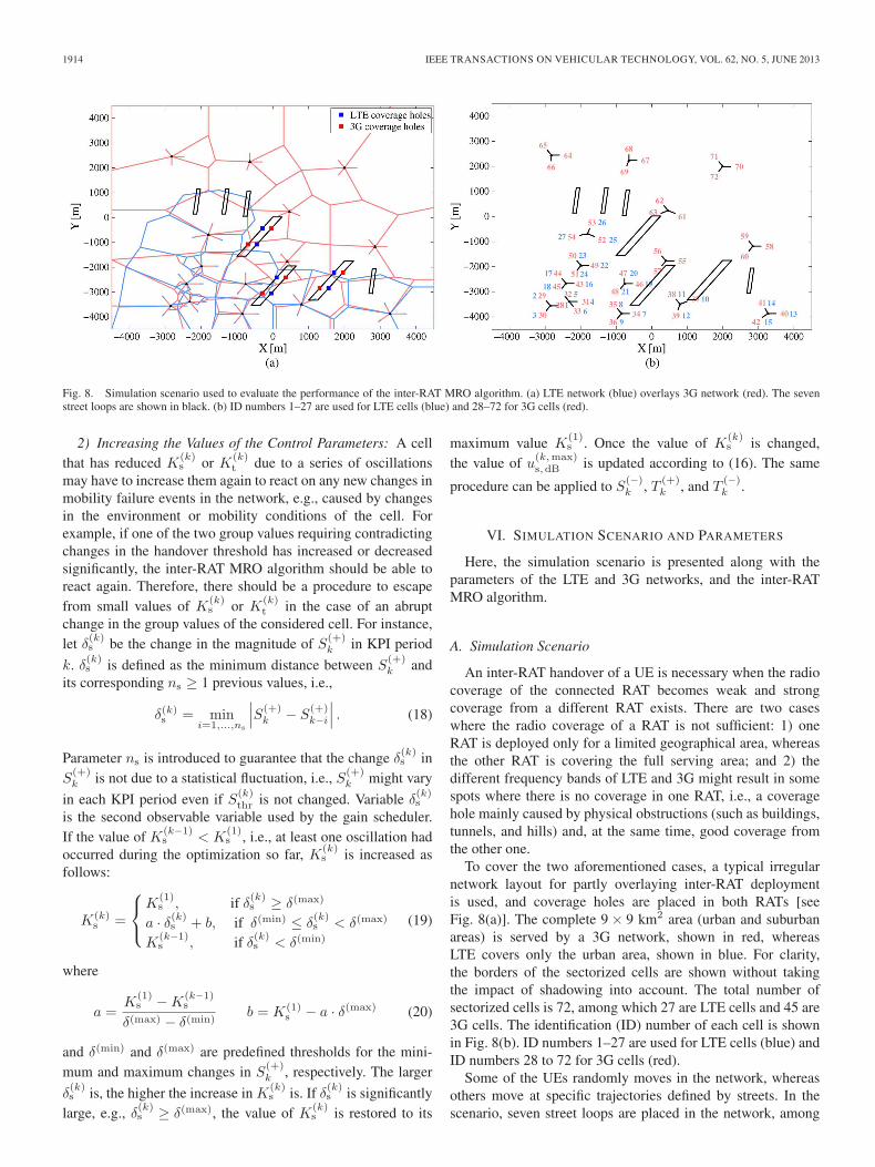
Fig. 8. Simulation scenario used to evaluate the performance of the inter-RAT MRO algorithm. (a) LTE network (blue) overlays 3G network (red). The sevenstreet loops are shown in black. (b) ID numbers 1–27 are used for LTE cells (blue) and 28–72 for 3G cells (red).

2) Increasing the Values of the Control Parameters: A cellthat has reduced K

(k)s or K

(k)t due to a series of oscillations

may have to increase them again to react on any new changes inmobility failure events in the network, e.g., caused by changesin the environment or mobility conditions of the cell. Forexample, if one of the two group values requiring contradictingchanges in the handover threshold has increased or decreasedsignificantly, the inter-RAT MRO algorithm should be able toreact again. Therefore, there should be a procedure to escapefrom small values of K

(k)s or K

(k)t in the case of an abrupt

change in the group values of the considered cell. For instance,let δ(k)s be the change in the magnitude of S(+)

k in KPI period

k. δ(k)s is defined as the minimum distance between S(+)k and

its corresponding ns ≥ 1 previous values, i.e.,

δ(k)s = mini=1,...,ns

∣∣∣S(+)k − S

(+)k−i

∣∣∣ . (18)

Parameter ns is introduced to guarantee that the change δ(k)s in

S(+)k is not due to a statistical fluctuation, i.e., S(+)

k might vary

in each KPI period even if S(k)thr is not changed. Variable δ

(k)s

is the second observable variable used by the gain scheduler.If the value of K(k−1)

s < K(1)s , i.e., at least one oscillation had

occurred during the optimization so far, K(k)s is increased as

follows:

K(k)s =

⎧⎨⎩

K(1)s , if δ(k)s ≥ δ(max)

a · δ(k)s + b, if δ(min) ≤ δ(k)s < δ(max)

K(k−1)s , if δ(k)s < δ(min)

(19)

where

a =K

(1)s −K

(k−1)s

δ(max) − δ(min)b = K(1)

s − a · δ(max) (20)

and δ(min) and δ(max) are predefined thresholds for the mini-mum and maximum changes in S

(+)k , respectively. The larger

δ(k)s is, the higher the increase in K

(k)s is. If δ(k)s is significantly

large, e.g., δ(k)s ≥ δ(max), the value of K(k)s is restored to its

maximum value K(1)s . Once the value of K

(k)s is changed,

the value of u(k,max)s,dB is updated according to (16). The same

procedure can be applied to S(−)k , T (+)

k , and T(−)k .

VI. SIMULATION SCENARIO AND PARAMETERS

Here, the simulation scenario is presented along with theparameters of the LTE and 3G networks, and the inter-RATMRO algorithm.

A. Simulation Scenario

An inter-RAT handover of a UE is necessary when the radiocoverage of the connected RAT becomes weak and strongcoverage from a different RAT exists. There are two caseswhere the radio coverage of a RAT is not sufficient: 1) oneRAT is deployed only for a limited geographical area, whereasthe other RAT is covering the full serving area; and 2) thedifferent frequency bands of LTE and 3G might result in somespots where there is no coverage in one RAT, i.e., a coveragehole mainly caused by physical obstructions (such as buildings,tunnels, and hills) and, at the same time, good coverage fromthe other one.

To cover the two aforementioned cases, a typical irregularnetwork layout for partly overlaying inter-RAT deploymentis used, and coverage holes are placed in both RATs [seeFig. 8(a)]. The complete 9 × 9 km2 area (urban and suburbanareas) is served by a 3G network, shown in red, whereasLTE covers only the urban area, shown in blue. For clarity,the borders of the sectorized cells are shown without takingthe impact of shadowing into account. The total number ofsectorized cells is 72, among which 27 are LTE cells and 45 are3G cells. The identification (ID) number of each cell is shownin Fig. 8(b). ID numbers 1–27 are used for LTE cells (blue) andID numbers 28 to 72 for 3G cells (red).

Some of the UEs randomly moves in the network, whereasothers move at specific trajectories defined by streets. In thescenario, seven street loops are placed in the network, among


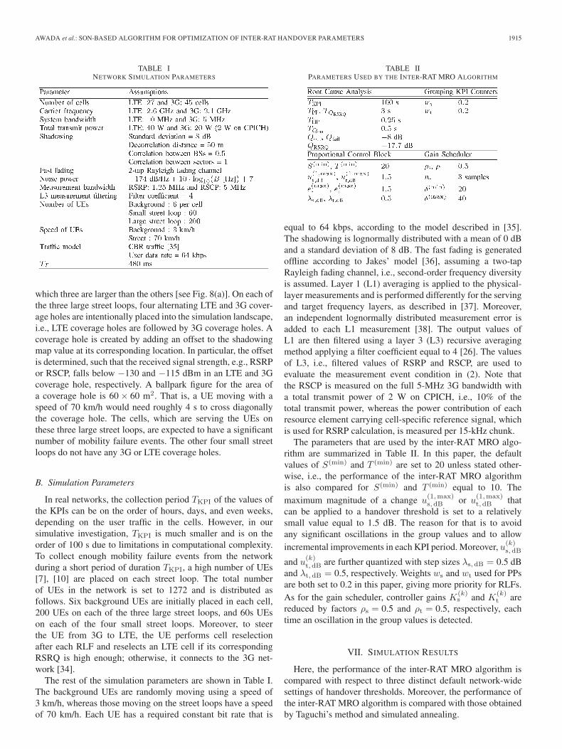
TABLE INETWORK SIMULATION PARAMETERS

which three are larger than the others [see Fig. 8(a)]. On each ofthe three large street loops, four alternating LTE and 3G cover-age holes are intentionally placed into the simulation landscape,i.e., LTE coverage holes are followed by 3G coverage holes. Acoverage hole is created by adding an offset to the shadowingmap value at its corresponding location. In particular, the offsetis determined, such that the received signal strength, e.g., RSRPor RSCP, falls below −130 and −115 dBm in an LTE and 3Gcoverage hole, respectively. A ballpark figure for the area ofa coverage hole is 60 × 60 m2. That is, a UE moving with aspeed of 70 km/h would need roughly 4 s to cross diagonallythe coverage hole. The cells, which are serving the UEs onthese three large street loops, are expected to have a significantnumber of mobility failure events. The other four small streetloops do not have any 3G or LTE coverage holes.

B. Simulation Parameters

In real networks, the collection period TKPI of the values ofthe KPIs can be on the order of hours, days, and even weeks,depending on the user traffic in the cells. However, in oursimulative investigation, TKPI is much smaller and is on theorder of 100 s due to limitations in computational complexity.To collect enough mobility failure events from the networkduring a short period of duration TKPI, a high number of UEs[7], [10] are placed on each street loop. The total numberof UEs in the network is set to 1272 and is distributed asfollows. Six background UEs are initially placed in each cell,200 UEs on each of the three large street loops, and 60s UEson each of the four small street loops. Moreover, to steerthe UE from 3G to LTE, the UE performs cell reselectionafter each RLF and reselects an LTE cell if its correspondingRSRQ is high enough; otherwise, it connects to the 3G net-work [34].

The rest of the simulation parameters are shown in Table I.The background UEs are randomly moving using a speed of3 km/h, whereas those moving on the street loops have a speedof 70 km/h. Each UE has a required constant bit rate that is

TABLE IIPARAMETERS USED BY THE INTER-RAT MRO ALGORITHM

equal to 64 kbps, according to the model described in [35].The shadowing is lognormally distributed with a mean of 0 dBand a standard deviation of 8 dB. The fast fading is generatedoffline according to Jakes’ model [36], assuming a two-tapRayleigh fading channel, i.e., second-order frequency diversityis assumed. Layer 1 (L1) averaging is applied to the physical-layer measurements and is performed differently for the servingand target frequency layers, as described in [37]. Moreover,an independent lognormally distributed measurement error isadded to each L1 measurement [38]. The output values ofL1 are then filtered using a layer 3 (L3) recursive averagingmethod applying a filter coefficient equal to 4 [26]. The valuesof L3, i.e., filtered values of RSRP and RSCP, are used toevaluate the measurement event condition in (2). Note thatthe RSCP is measured on the full 5-MHz 3G bandwidth witha total transmit power of 2 W on CPICH, i.e., 10% of thetotal transmit power, whereas the power contribution of eachresource element carrying cell-specific reference signal, whichis used for RSRP calculation, is measured per 15-kHz chunk.

The parameters that are used by the inter-RAT MRO algo-rithm are summarized in Table II. In this paper, the defaultvalues of S(min) and T (min) are set to 20 unless stated other-wise, i.e., the performance of the inter-RAT MRO algorithmis also compared for S(min) and T (min) equal to 10. Themaximum magnitude of a change u

(1,max)s,dB or u

(1,max)t,dB that

can be applied to a handover threshold is set to a relativelysmall value equal to 1.5 dB. The reason for that is to avoidany significant oscillations in the group values and to allowincremental improvements in each KPI period. Moreover, u(k)

s,dB

and u(k)t,dB are further quantized with step sizes λs,dB = 0.5 dB

and λt,dB = 0.5, respectively. Weights ws and wt used for PPsare both set to 0.2 in this paper, giving more priority for RLFs.As for the gain scheduler, controller gains K

(k)s and K

(k)t are

reduced by factors ρs = 0.5 and ρt = 0.5, respectively, eachtime an oscillation in the group values is detected.

VII. SIMULATION RESULTS

Here, the performance of the inter-RAT MRO algorithm iscompared with respect to three distinct default network-widesettings of handover thresholds. Moreover, the performance ofthe inter-RAT MRO algorithm is compared with those obtainedby Taguchi’s method and simulated annealing.


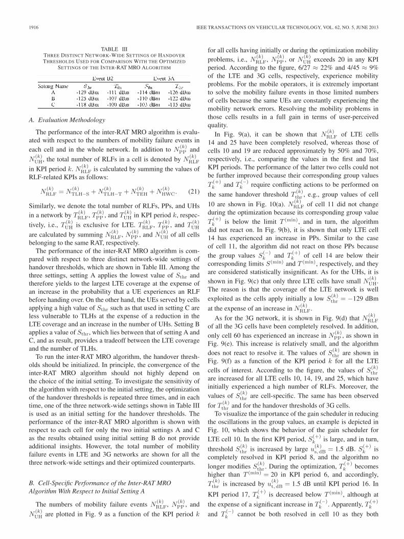
TABLE IIITHREE DISTINCT NETWORK-WIDE SETTINGS OF HANDOVER

THRESHOLDS USED FOR COMPARISON WITH THE OPTIMIZED

SETTINGS OF THE INTER-RAT MRO ALGORITHM

A. Evaluation Methodology

The performance of the inter-RAT MRO algorithm is evalu-ated with respect to the numbers of mobility failure events ineach cell and in the whole network. In addition to N

(k)PP and

N(k)UH, the total number of RLFs in a cell is denoted by N

(k)RLF

in KPI period k. N (k)RLF is calculated by summing the values of

RLF-related KPIs as follows:

N(k)RLF = N

(k)TLH−S +N

(k)TLH−T +N

(k)TEH +N

(k)HWC. (21)

Similarly, we denote the total number of RLFs, PPs, and UHsin a network by T

(k)RLF, T (k)

PP , and T(k)UH in KPI period k, respec-

tively, i.e., T (k)UH is exclusive for LTE. T (k)

RLF, T (k)PP , and T

(k)UH

are calculated by summing N(k)RLF, N (k)

PP , and N(k)UH of all cells

belonging to the same RAT, respectively.The performance of the inter-RAT MRO algorithm is com-

pared with respect to three distinct network-wide settings ofhandover thresholds, which are shown in Table III. Among thethree settings, setting A applies the lowest value of Sthr andtherefore yields to the largest LTE coverage at the expense ofan increase in the probability that a UE experiences an RLFbefore handing over. On the other hand, the UEs served by cellsapplying a high value of Sthr such as that used in setting C areless vulnerable to TLHs at the expense of a reduction in theLTE coverage and an increase in the number of UHs. Setting Bapplies a value of Sthr, which lies between that of setting A andC, and as result, provides a tradeoff between the LTE coverageand the number of TLHs.

To run the inter-RAT MRO algorithm, the handover thresh-olds should be initialized. In principle, the convergence of theinter-RAT MRO algorithm should not highly depend onthe choice of the initial setting. To investigate the sensitivity ofthe algorithm with respect to the initial setting, the optimizationof the handover thresholds is repeated three times, and in eachtime, one of the three network-wide settings shown in Table IIIis used as an initial setting for the handover thresholds. Theperformance of the inter-RAT MRO algorithm is shown withrespect to each cell for only the two initial settings A and Cas the results obtained using initial setting B do not provideadditional insights. However, the total number of mobilityfailure events in LTE and 3G networks are shown for all thethree network-wide settings and their optimized counterparts.

B. Cell-Specific Performance of the Inter-RAT MROAlgorithm With Respect to Initial Setting A

The numbers of mobility failure events N(k)RLF, N (k)

PP , and

N(k)UH are plotted in Fig. 9 as a function of the KPI period k

for all cells having initially or during the optimization mobilityproblems, i.e., N (k)

RLF, N (k)PP , or N

(k)UH exceeds 20 in any KPI

period. According to the figure, 6/27 ≈ 22% and 4/45 ≈ 9%of the LTE and 3G cells, respectively, experience mobilityproblems. For the mobile operators, it is extremely importantto solve the mobility failure events in those limited numbersof cells because the same UEs are constantly experiencing themobility network errors. Resolving the mobility problems inthose cells results in a full gain in terms of user-perceivedquality.

In Fig. 9(a), it can be shown that N(k)RLF of LTE cells

14 and 25 have been completely resolved, whereas those ofcells 10 and 19 are reduced approximately by 50% and 70%,respectively, i.e., comparing the values in the first and lastKPI periods. The performance of the latter two cells could notbe further improved because their corresponding group valuesT

(+)k and T

(−)k require conflicting actions to be performed on

the same handover threshold T(k)thr , e.g., group values of cell

10 are shown in Fig. 10(a). N (k)RLF of cell 11 did not change

during the optimization because its corresponding group valueT

(+)k is below the limit T (min), and in turn, the algorithm

did not react on. In Fig. 9(b), it is shown that only LTE cell14 has experienced an increase in PPs. Similar to the caseof cell 11, the algorithm did not react on those PPs becausethe group values S

(−)k and T

(+)k of cell 14 are below their

corresponding limits S(min) and T (min), respectively, and theyare considered statistically insignificant. As for the UHs, it isshown in Fig. 9(c) that only three LTE cells have small N (k)

UH.The reason is that the coverage of the LTE network is wellexploited as the cells apply initially a low S

(k)thr = −129 dBm

at the expense of an increase in N(k)RLF.

As for the 3G network, it is shown in Fig. 9(d) that N (k)RLF

of all the 3G cells have been completely resolved. In addition,only cell 60 has experienced an increase in N

(k)PP , as shown in

Fig. 9(e). This increase is relatively small, and the algorithmdoes not react to resolve it. The values of S

(k)thr are shown in

Fig. 9(f) as a function of the KPI period k for all the LTEcells of interest. According to the figure, the values of S

(k)thr

are increased for all LTE cells 10, 14, 19, and 25, which haveinitially experienced a high number of RLFs. Moreover, thevalues of S

(k)thr are cell-specific. The same has been observed

for T (k)thr and for the handover thresholds of 3G cells.

To visualize the importance of the gain scheduler in reducingthe oscillations in the group values, an example is depicted inFig. 10, which shows the behavior of the gain scheduler forLTE cell 10. In the first KPI period, S(+)

k is large, and in turn,

threshold S(k)thr is increased by large u

(k)s,dB = 1.5 dB. S(+)

k iscompletely resolved in KPI period 8, and the algorithm nolonger modifies S

(k)thr . During the optimization, T (+)

k becomeshigher than T (min) = 20 in KPI period 6, and accordingly,T

(k)thr is increased by u

(k)t,dB = 1.5 dB until KPI period 16. In

KPI period 17, T (+)k is decreased below T (min), although at

the expense of a significant increase in T(−)k . Apparently, T (+)

k

and T(−)k cannot be both resolved in cell 10 as they both


Fig. 9. Performance of the inter-RAT MRO algorithm with respect to initial setting A. (a) Number of RLFs in LTE cells. (b) Number of PPs in LTE cells.

(c) Number of UHs in LTE cells. (d) Number of RLFs in 3G cells. (e) Number of PPs in 3G cells. (f) S(k)thr

of LTE cells as a function of k.

Fig. 10. Example showing the role of the gain scheduler in reducing the oscillations in the group values of cell 10. (a) Group values of cell 10 as a function of

the KPI period k. (b) Values of u(k)s, dB

and u(k)t, dB

applied by cell 10 to S(k)thr

and T(k)thr

, respectively, and their corresponding controller gains K(k)s and K

(k)t as a

function of the KPI period k.

require conflicting actions to be performed on T(k)thr . In KPI

period 18, the gain scheduler detects an oscillation in T(+)k and

T(−)k and in turn reduces the controller gain K

(k)t by half. The

gain scheduler detects a new oscillation in KPI period 19 andreduces furthermore K

(k)t . As a result, the magnitude of u(k)

t,dB

is reduced from 1.5 dB in KPI period 16 to 0.5 dB in KPIperiod 18, and to 0 dB in KPI period 19. Therefore, the gainscheduler has gradually learned via detecting the oscillationsthat a small or no change should be applied to T

(k)thr . In KPI

period 21, the small change in T(k)thr yielded again a significant

increase in T(−)k , i.e., δ(21)>δ(max), and the gain scheduler res-

tores K(k)t to its maximum value to react on the new mobility

failure events. Shortly after, the gain scheduler detects two

oscillations in KPI periods 22 and 23, and reduces again K(k)t

to 0.25. The handover thresholds are not changed in the lastfive KPI periods, and in turn, stability is achieved in the groupvalues. Without the gain scheduler, T

(+)k and T

(−)k would

infinitely oscillate, and stability would not be reached.

C. Cell-Specific Performance of the Inter-RAT MROAlgorithm With Respect to Initial Setting C

The number of mobility failure events N (k)RLF, N (k)

PP , and N(k)UH

are plotted in Fig. 11 as a function of the KPI period k forall cells having initially or during the optimization mobilityproblems. In contrast to initial setting A, the number of LTEcells having significant N (k)

RLF in the first KPI period is smaller


Fig. 11. Performance of the inter-RAT MRO algorithm with respect to initial setting C. (a) Number of RLFs in LTE cells. (b) Number of PPs in LTE cells.

(c) Number of UHs in LTE cells. (d) Number of RLFs in 3G cells. (e) Number of PPs in 3G cells. (f) S(k)thr

of LTE cells as a function of k.

Fig. 12. Performance of the inter-RAT MRO algorithm applying initial setting C for two different values of S(min) and T (min). (a) Number of RLFs.(b) Number of PPs. (c) Number of UHs.

at the expense of an increase in the number of cells having highN

(k)UH. The reason is that LTE cells initially apply high S

(k)thr =

−118 dBm and in turn are less affected by RLFs at the expenseof a reduction in LTE coverage and an increase in N

(k)UH.

In Fig. 11(a), it is shown that N (k)RLF is reduced for LTE cell

25, whereas the performance of cells 10 and 19 could not beimproved as their corresponding group values T

(+)k and T

(−)k

require contradicting actions to be performed on T(k)thr . The rest

of the LTE cells have small N (k)RLF values, which are not large

enough for the algorithm to react on. N (k)PP of LTE cells 19 and

25 have increased, as shown in Fig. 11(b); however, the algo-rithm did not react on them because their corresponding groupvalues did not exceed the minimum limits S(min) and T (min).The inter-RAT MRO algorithm completely resolves the UHs ofsix LTE cells, as shown in Fig. 11(c). To this end, S(k)

thr of thelatter LTE cells were decreased cell-specifically, as shown inFig. 11(f), and consequently, the LTE coverage is expanded. Asfor the 3G network, N (k)

RLF of the 3G cells shown in Fig. 11(d)

have been completely resolved without any significant increasein the number of PPs, as shown in Fig. 11(e).

To investigate the impact of thresholds S(min) and T (min) onthe performance of the inter-RAT MRO algorithm, we comparein Fig. 12 the numbers of RLFs, PPs, and UHs of all cells in thelast KPI period 28 for two threshold values: S(min) and T (min)

are both set either to 10 or 20. According to the figure, it isshown that the latter two threshold values do not have an impacton cells 10, 11, 20, 57, 60, and 63, where similar numbers ofmobility failures are achieved. Cells 26 and 37 have less RLFsfor S(min) and T (min) equal to 10 at the expense of a slight lossin UHs for cell 26. Moreover, the number of PPs has decreasedin cell 25, whereas the number of UHs has increased in cell14. As for cell 19, the number of PPs has decreased from 77to 8, i.e., a gain of (77 − 8) · (ws + wt) = 27.6 in PPs, at theexpense of an increase in RLFs from 27 to 49, i.e., a loss of 22 inRLFs. Therefore, the impact of the values of S(min) and T (min)

on the overall performance of the inter-RAT MRO algorithm ismore or less minimal as long as they are reasonably configured.


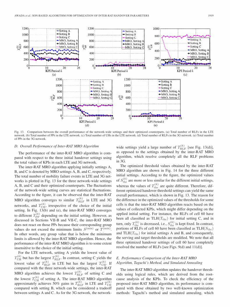
Fig. 13. Comparison between the overall performance of the network-wide settings and their optimized counterparts. (a) Total number of RLFs in the LTEnetwork. (b) Total number of PPs in the LTE network. (c) Total number of UHs in the LTE network. (d) Total number of RLFs in the 3G network. (e) Total numberof PPs in the 3G network.

D. Overall Performance of Inter-RAT MRO Algorithm

The performance of the inter-RAT MRO algorithm is com-pared with respect to the three initial handover settings usingthe total values of KPIs in each LTE and 3G network.

The inter-RAT MRO algorithm applying initially settings A,B, and C is denoted by MRO settings A, B, and C, respectively.The total number of mobility failure events in LTE and 3G net-works is plotted in Fig. 13 for the three network-wide settingsA, B, and C and their optimized counterparts. The fluctuationsof the network-wide setting curves are statistical fluctuations.According to the figure, it can be observed that the inter-RATMRO algorithm converges to similar T

(k)RLF in LTE and 3G

networks, and T(k)UH , irrespective of the choice of the initial

setting. In Fig. 13(b) and (e), the inter-RAT MRO convergesto different T (k)

PP depending on the initial setting. However, asdiscussed in Sections VII-B and VII-C, the inter-RAT MROdoes not react on those PPs because their corresponding groupvalues do not exceed the minimum limits S(min) or T (min).In other words, any group value that is below the minimumlimits is allowed by the inter-RAT MRO algorithm. Hence, theperformance of the inter-RAT MRO algorithm is to some extentinsensitive to the choice of the initial setting.

For the LTE network, setting A yields the lowest value ofT

(k)UH but has the largest T (k)

RLF. In contrast, setting C yields the

lowest value of T(k)RLF in LTE but has the largest T

(k)UH . If

compared with the three network-wide settings, the inter-RATMRO algorithm achieves the lowest T

(k)RLF of setting C and

the lowest T (k)UH of setting A. The inter-RAT MRO algorithm

approximately achieves 50% gains in T(k)RLF in LTE and T

(k)UH

compared with setting B, which can be considered a tradeoffbetween settings A and C. As for the 3G network, the network-

wide settings yield a large number of T(k)RLF [see Fig. 13(d)],

as opposed to the settings obtained by the inter-RAT MROalgorithm, which resolve completely all the RLF problemsin 3G.

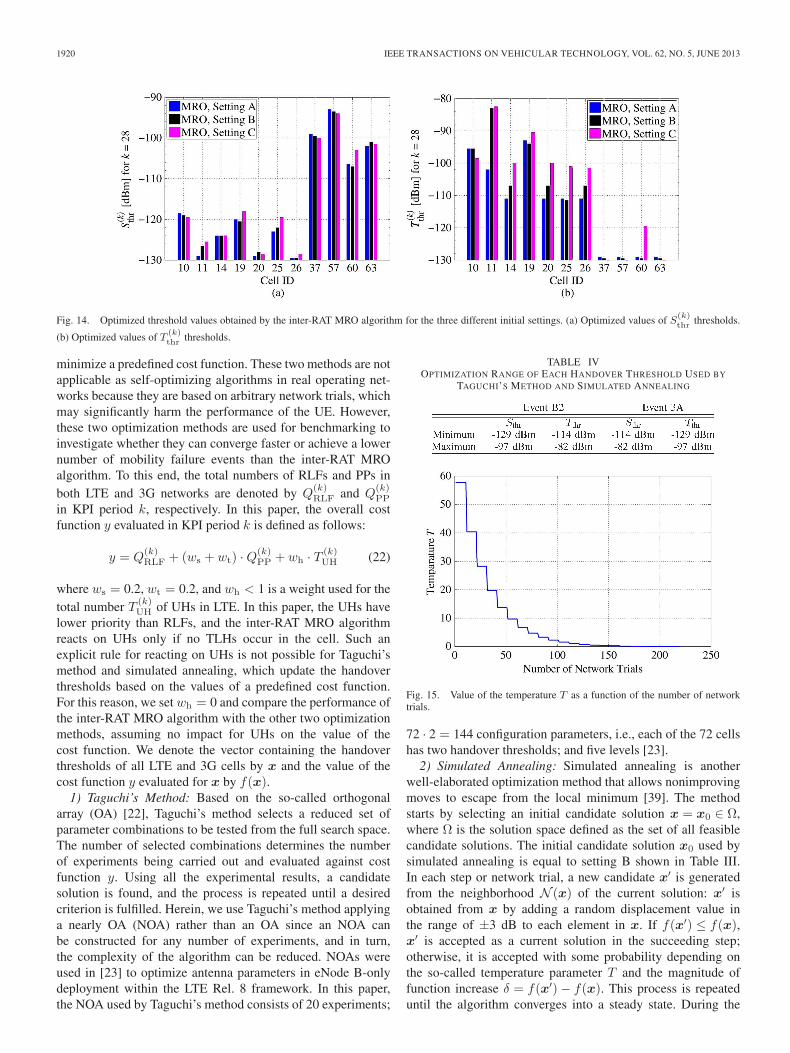
The optimized threshold values obtained by the inter-RATMRO algorithm are shown in Fig. 14 for the three differentinitial settings. According to the figure, the optimized valuesof S(k)

thr are more or less similar for the different initial settings,

whereas the values of T (k)thr are quite different. Therefore, dif-

ferent optimized handover threshold settings can yield the sameoverall performance, which is shown in Fig. 13. The reason forthe difference in the optimized values of the thresholds for somecells is that the inter-RAT MRO algorithm reacts based on thevalues of collected KPIs, which might differ depending on theapplied initial setting. For instance, the RLFs of cell 60 havebeen all classified as TLH(Tthr) for initial setting C, and inturn, only T

(k)thr is decreased, i.e., S(k)

thr is kept fixed. In contrast,portions of RLFs of cell 60 have been classified as TLH(Sthr)and TLH(Tthr) for initial settings A and B, and consequently,the serving and target thresholds are modified. We note that allthree optimized handover settings of cell 60 have completelyresolved the number of RLFs [see Figs. 9(d) and 11(d)].

E. Performance Comparison of the Inter-RAT MROAlgorithm, Taguchi’s Method, and Simulated Annealing

The inter-RAT MRO algorithm updates the handover thresh-olds using logical rules, which are derived from the root-cause analysis of the KPIs. To check the efficiency of theproposed inter-RAT MRO algorithm, its performance is com-pared with those obtained by two well-known optimizationmethods: Taguchi’s method and simulated annealing, which


Fig. 14. Optimized threshold values obtained by the inter-RAT MRO algorithm for the three different initial settings. (a) Optimized values of S(k)thr

thresholds.

(b) Optimized values of T (k)thr

thresholds.

minimize a predefined cost function. These two methods are notapplicable as self-optimizing algorithms in real operating net-works because they are based on arbitrary network trials, whichmay significantly harm the performance of the UE. However,these two optimization methods are used for benchmarking toinvestigate whether they can converge faster or achieve a lowernumber of mobility failure events than the inter-RAT MROalgorithm. To this end, the total numbers of RLFs and PPs inboth LTE and 3G networks are denoted by Q

(k)RLF and Q

(k)PP

in KPI period k, respectively. In this paper, the overall costfunction y evaluated in KPI period k is defined as follows:

y = Q(k)RLF + (ws + wt) ·Q(k)

PP + wh · T (k)UH (22)

where ws = 0.2, wt = 0.2, and wh < 1 is a weight used for thetotal number T (k)

UH of UHs in LTE. In this paper, the UHs havelower priority than RLFs, and the inter-RAT MRO algorithmreacts on UHs only if no TLHs occur in the cell. Such anexplicit rule for reacting on UHs is not possible for Taguchi’smethod and simulated annealing, which update the handoverthresholds based on the values of a predefined cost function.For this reason, we set wh = 0 and compare the performance ofthe inter-RAT MRO algorithm with the other two optimizationmethods, assuming no impact for UHs on the value of thecost function. We denote the vector containing the handoverthresholds of all LTE and 3G cells by x and the value of thecost function y evaluated for x by f(x).

1) Taguchi’s Method: Based on the so-called orthogonalarray (OA) [22], Taguchi’s method selects a reduced set ofparameter combinations to be tested from the full search space.The number of selected combinations determines the numberof experiments being carried out and evaluated against costfunction y. Using all the experimental results, a candidatesolution is found, and the process is repeated until a desiredcriterion is fulfilled. Herein, we use Taguchi’s method applyinga nearly OA (NOA) rather than an OA since an NOA canbe constructed for any number of experiments, and in turn,the complexity of the algorithm can be reduced. NOAs wereused in [23] to optimize antenna parameters in eNode B-onlydeployment within the LTE Rel. 8 framework. In this paper,the NOA used by Taguchi’s method consists of 20 experiments;

TABLE IVOPTIMIZATION RANGE OF EACH HANDOVER THRESHOLD USED BY

TAGUCHI’S METHOD AND SIMULATED ANNEALING

Fig. 15. Value of the temperature T as a function of the number of networktrials.

72 · 2 = 144 configuration parameters, i.e., each of the 72 cellshas two handover thresholds; and five levels [23].

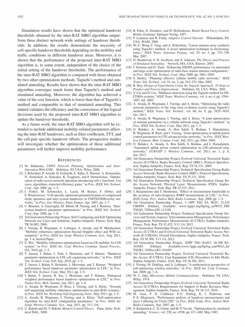
2) Simulated Annealing: Simulated annealing is anotherwell-elaborated optimization method that allows nonimprovingmoves to escape from the local minimum [39]. The methodstarts by selecting an initial candidate solution x = x0 ∈ Ω,where Ω is the solution space defined as the set of all feasiblecandidate solutions. The initial candidate solution x0 used bysimulated annealing is equal to setting B shown in Table III.In each step or network trial, a new candidate x′ is generatedfrom the neighborhood N (x) of the current solution: x′ isobtained from x by adding a random displacement value inthe range of ±3 dB to each element in x. If f(x′) ≤ f(x),x′ is accepted as a current solution in the succeeding step;otherwise, it is accepted with some probability depending onthe so-called temperature parameter T and the magnitude offunction increase δ = f(x′)− f(x). This process is repeateduntil the algorithm converges into a steady state. During the


Fig. 16. Comparison between the cost functions achieved by the inter-RAT MRO algorithm applying initial setting B and those obtained by Taguchi’s methodand simulated annealing. (a) Cost function y as a function of the number of network trials for the inter-RAT MRO algorithm applying initial setting B and Taguchi’smethod. (b) Cost function y as a function of the number of network trials for the inter-RAT MRO algorithm applying initial setting B and simulated annealing.

search, temperature T is slowly decreased using a standardgeometric temperature reduction function ρ(T ) = κ · T as in[19], where κ is a reduction ratio that is set to 0.7. The initialvalue of T , denoted by T0, is selected such that an increaseof 40 in the cost function is accepted at the beginning with aprobability of 0.5, i.e., T0 = 40/ log(0.5) [23]. The value of Tis shown in Fig. 15 as a function of the number of networktrials.

3) Performance Evaluation: The optimization range of eachhandover threshold used by Taguchi’s method and simulatedannealing is shown in Table IV.

The optimization range is defined such that it includesthe optimized values of the handover thresholds obtainedby the inter-RAT MRO algorithm applying initial setting B.In the case of Taguchi’s method, cost function y is evaluatedin each experiment, which is equivalent to one network trial.Therefore, one network trial performed by Taguchi’s methodis equivalent to one evaluation f(x) of the cost function per-formed by simulated annealing. For both methods, cost functiony is evaluated using the values of the KPIs collected from bothLTE and 3G networks during the same TKPI time interval usedfor the inter-RAT MRO algorithm. As for the inter-RAT MROalgorithm, a new set of handover thresholds is selected in eachKPI period. Therefore, each KPI period also corresponds to onenetwork trial.

In Fig. 16, cost function y is plotted as a function of thenumber of network trials for the inter-RAT MRO algorithmapplying initial setting B, Taguchi’s method in Fig. 16(a), andsimulated annealing in Fig. 16(b). The red line indicates thevalue of the cost function evaluated in the first KPI periodfor the network-wide setting B. The blue line determines theminimum value of the cost function that the inter-RAT MROalgorithm applying initial setting B converges to during theoptimization. Simulated annealing has the same cost functionof the inter-RAT MRO algorithm in the first KPI period sinceit applies setting B as initial candidate solution x0. However,Taguchi’s method does not have any initial setting [23], andin turn, the value of its cost function in the first KPI period isdifferent than those of simulated annealing and the inter-RATMRO algorithm.

According to Fig. 16, it is shown that the inter-RAT MROalgorithm has a much faster convergence than Taguchi’s methodand simulated annealing. This is because the inter-RAT MROdirectly reacts on the handover thresholds of the cells havingmobility problems, whereas the two other methods explorefirst the predefined optimization range of the handover thresh-old before converging. Moreover, the minimum values of thecost functions achieved by the inter-RAT MRO algorithm,Taguchi’s method, and simulated annealing are 73.3%, 52.7%,and 71.49% lower than the cost function of the network-wide setting B shown by the red line, respectively. Therefore,the inter-RAT MRO algorithm outperforms in this scenarioTaguchi’s method and provides comparable results to simulatedannealing. This result, indeed, shows that the logical decisionsthat are used by the inter-RAT MRO algorithm to adjust thehandover thresholds are appropriate and efficient.

VIII. CONCLUSION AND OUTLOOK

In this paper, a SON-based algorithm for optimizing inter-RAT handover thresholds has been presented. The algorithmruns on both LTE and 3G networks. The inter-RAT KPIs aredefined and the root cause of each mobility failure event isdetermined. An inter-RAT handover is triggered by a dual-threshold measurement event where the first threshold corre-sponds to the serving cell and the second threshold to theneighboring target cell of another RAT. As a result, there aretwo types of too-late handovers in contrast to the intra-RATcase, where a single type of too-late handover exists. The valuesof the inter-RAT KPIs are collected from each cell in both RATsand are further mapped into four new other values dependingon the action required by each mobility failure event, i.e.,increasing or decreasing a handover threshold. Modifying thehandover thresholds by a fixed and large step size may lead tofluctuations in the values of the KPIs and, in turn, instabilityin the network. As a countermeasure, a proportional feedbackcontroller is used to apply the necessary amount of change toeach handover threshold. Moreover, a gain scheduler is added toadjust the parameters of the controller according to the mobilityconditions of each cell.


Simulation results have shown that the optimized handoverthresholds obtained by the inter-RAT MRO algorithm outper-form three distinct network-wide settings of handover thresh-olds. In addition, the results demonstrate the necessity ofcell-specific handover thresholds depending on the mobility andtraffic conditions in different handover areas. Moreover, it isshown that the performance of the proposed inter-RAT MROalgorithm is, to some extent, independent of the choice of theinitial setting of the handover thresholds. The performance ofthe inter-RAT MRO algorithm is compared with those obtainedby two other optimization methods: Taguchi’s method and sim-ulated annealing. Results have shown that the inter-RAT MROalgorithm converges much faster than Taguchi’s method andsimulated annealing. Moreover, the algorithm has achieved avalue of the cost function, which is lower than that of Taguchi’smethod and comparable to that of simulated annealing. Thisindeed validates the efficiency and the correctness of the logicaldecisions used by the proposed inter-RAT MRO algorithm toupdate the handover thresholds.

As a future work, the inter-RAT MRO algorithm will be ex-tended to include additional mobility-related parameters affect-ing the inter-RAT handovers, such as filter coefficient, TTT, andthe cell-pair specific handover offsets. The prospective studieswill investigate whether the optimization of these additionalparameters will further improve mobility performance.

REFERENCES

[1] M. Rahnema, UMTS Network Planning, Optimization and Inter-Operation With GSM. Hoboken, NJ, USA: Wiley, 2008.

[2] J. Belschner, P. Arnold, H. Eckhardt, E. Kuhn, E. Patouni, A. Kousaridas,N. Alonistioti, A. Saatsakis, K. Tsagkaris, and P. Demestichas, “Optimi-sation of radio access network operation introducing self-x functions: Usecases, algorithms, expected efficiency gains,” in Proc. IEEE Veh. Technol.Conf., Apr. 2009, pp. 1–5.

[3] I. Forkel, M. Schmocker, L. Lazin, M. Becker, F. Debus, andF. Winnewisser, “Cell-specific optimized parameterization of compressedmode operation and inter-system handovers in UMTS/GSMoverlay net-works,” in Proc. Eur. Wireless, Paris, France, Apr. 2007, pp. 1–7.

[4] C. Brunner, A. Garavaglia, M. Mittal, M. Narang, and J. Bautista, “Inter-system handover parameter optimization,” in Proc. IEEE Veh. Technol.Conf., Sep. 2006, pp. 1–6.

[5] 3rd Generation Partnership Project, Self-Configuring and Self-OptimizingNetwork use Cases and Solutions, Sophia-Antipolis, France, Tech. Rep.TR 36.902, 2009.

[6] I. Viering, B. Wegmann, A. Lobinger, A. Awada, and H. Martikainen,“Mobility robustness optimization beyond Doppler effect and WSS as-sumption,” in Proc. IEEE Int. Symp. Wireless Commun. Syst., Aug. 2011,pp. 1–6, Invited Paper.

[7] Z. Wei, “Mobility robustness optimization based on UE mobility for LTEsystem,” in Proc. IEEE Int. Conf. Wireless Commun. Signal Process.,Oct. 2010, pp. 1–5.

[8] T. Jansen, I. Balan, J. Turk, I. Moerman, and T. Kürner, “Handoverparameter optimization in LTE self-organizing networks,” in Proc. IEEEVeh. Technol. Conf. Fall, Sep. 2010, pp. 1–5.

[9] T. Jansen, I. Balan, S. Stefanski, I. Moerman, and T. Kürner, “Weightedperformance based handover parameter optimization in LTE,” in Proc.IEEE Veh. Technol. Conf., May 2011, pp. 1–5.

[10] I. Balan, T. Jansen, B. Sas, I. Moerman, and T. Kürner, “Enhancedweighted performance based handover optimization in LTE,” in Proc.Future Netw. Mob. Summit, Jun. 2011, pp. 1–8.

[11] A. Awada, B. Wegmann, D. Rose, I. Viering, and A. Klein, “Towardsself-organizing mobility robustness optimization in inter-RAT scenario,”in Proc. IEEE Int. Workshop Self-Organizing Netw., May 2011, pp. 1–5.

[12] A. Awada, B. Wegmann, I. Viering, and A. Klein, “Self-optimizationalgorithm for inter-RAT configuration parameters,” in Proc. IEEE Int.Symp. Wireless Commun. Syst., Aug. 2011, pp. 311–316.

[13] U. Bakshi and M. V. Bakshi, Modern Control Theory. Pune, India: Tech-nical Publ., 2008.

[14] R. Palm, D. Driankov, and H. Hellendoorn, Model Based Fuzzy Control.Berlin, Germany: Springer-Verlag, 1997.

[15] P. Loannou and B. Fidan, Adaptive Control Tutorial. Philadelphia, PA,USA: SIAM, 2006.

[16] W.-C. Weng, F. Yang, and A. Elsherbeni, “Linear antenna array synthesisusing Taguchi’s method: A novel optimization technique in electromag-netics,” IEEE Trans. Antennas Propag., vol. 55, no. 3, pp. 723–730,Mar. 2007.

[17] D. Henderson, S. H. Jacobson, and A. Johnson, The Theory and Practiceof Simulated Annealing. Norwell, MA, USA: Kluwer, 2003.

[18] I. Siomina and D. Yuan, “Enhancing HSDPA performance via automatedand large-scale optimization of radio base station antenna configuration,”in Proc. IEEE Veh. Technol. Conf., May 2008, pp. 2061–2065.

[19] S. Hurley, “Planning effective cellular mobile radio networks,” IEEETrans. Veh. Technol., vol. 51, no. 2, pp. 243–253, Mar. 2002.

[20] R. Roy, Design of Experiments Using the Taguchi Approach: 16 Steps toProduct and Process Improvement. Hoboken, NJ, USA: Wiley, 2001.

[21] Y. Cai and D. Liu, “Multiuser detection using the Taguchi method for DS-CDMA systems,” IEEE Trans. Wireless Commun., vol. 4, no. 4, pp. 1594–1607, Jul. 2005.

[22] A. Awada, B. Wegmann, I. Viering, and A. Klein, “Optimizing the radionetwork parameters of the long term evolution system using Taguchi’smethod,” IEEE Trans. Veh. Technol., vol. 60, no. 8, pp. 3825–3839,Oct. 2011.

[23] A. Awada, B. Wegmann, I. Viering, and A. Klein, “A joint optimizationof antenna parameters in a cellular network using Taguchi’s method,” inProc. IEEE Veh. Technol. Conf., May 2011, pp. 1–5.

[24] O. Bulakci, A. Awada, A. Bou Saleh, S. Redana, J. Hamalainen,B. Wegmann, B. Raaf, and I. Viering, “Joint optimization of uplink powercontrol parameters in LTE-advanced relay networks,” in Proc. IEEE Wire-less Commun. Mob. Comput. Conf., July 2011, pp. 2064–2069.

[25] O. Bulakci, A. Awada, A. Bou Saleh, S. Redana, and J. Hamalainen,“Automated uplink power control optimization in LTE-advanced relaynetworks,” EURASIP J. Wireless Commun., vol. 2013, no. 1, p. 8,Jan. 2013.

[26] 3rd Generation Partnership Project, Evolved Universal Terrestrial RadioAccess (E-UTRA); Radio Resource Control (RRC); Protocol Specifica-tion, Sophia-Antipolis, France, Tech. Rep. TS 36.331, 2009.

[27] 3rd Generation Partnership Project,Technical Specification Group RadioAccess Network; Radio Resource Control (RRC); Protocol Specification,Sophia-Antipolis, France, Tech. Rep. TS 25.331, 2010.

[28] 3rd Generation Partnership Project, Technical Specification Group Ra-dio Access Network; Physical Layer; Measurements (FDD), Sophia-Antipolis, France, Tech. Rep. TR 25.215, 2011.

[29] J. Kurjenniemi and T. Henttonen, “Effect of measurement bandwidth tothe accuracy of inter-frequency RSRP measurements in LTE,” in Proc.IEEE Symp. Pers., Indoor Mob. Radio Commun., Sep. 2008, pp. 1–5.

[30] 3rd Generation Partnership Project, 3 GPP TSG SA WG5, 32.425CR0089. [Online]. Available: www.3gpp1.org/ftp/tsg_sa/WG5_TM/TSGS5_79/Docs/S5-113108

[31] 3rd Generation Partnership Project, Technical Specification Group Ser-vices and System Aspects; Telecommnication Management, PerformanceManagement; Performance Measurements (E-UTRA), Sophia-Antipolis,France, Tech. Rep. TS 32.425, V11.3.0, 2012.

[32] 3rd Generation Partnership Project, Evolved Universal Terrestrial RadioAccess (E-UTRA) and Evolved Universal Terrestrial Radio Access Net-work (E-UTRAN); Overall Description, Sophia-Antipolis, France, Tech.Rep. TS 36.300, V11.3.0, 2012.

[33] 3rd Generation Partnership Project, 3GPP TSG RAN3, 36.300 R3-103485. [Online]. Available:www.3gpp.org/ftp/tsg_ran/WG3_Iu/TSGR3_70/Docs/R3-103485

[34] 3rd Generation Partnership Project, Evolved Universal Terrestrial Ra-dio Access (E-UTRA); User Equipment (UE) Procedures in Idle Mode,Sophia-Antipolis, France, Tech. Rep. TS 36.304, 2011.

[35] I. Viering, M. Döttling, and A. Lobinger, “A mathemetical perspective ofself-optimizing wireless networks,” in Proc. IEEE Int. Conf. Commun.,Jun. 2009, pp. 1–6.

[36] W. C. Jake, Microwave Mobile Communications. Hoboken, NJ, USA:Wiley, 1974.

[37] 3rd Generation Partnership Project, Evolved Universal Terrestrial RadioAccess (E-UTRA); Requirements for Support of Radio Resource Man-agement, Sophia-Antipolis, France, Tech. Rep. TS 36.133, 2010.

[38] M. Anas, F. D. Calabrese, P.-E. Östling, K. I. Pederson, andP. E. Mogensen, “Performance analysis of handover measurements andlayer 3 filtering for Utran LTE,” in Proc. IEEE Symp. Pers., Indoor Mob.Radio Commun., Sep. 2007, pp. 1–5.

[39] S. Kirkpatrick, C. D. Gelatt, and M. P. Vecchi, “Optimization by simulatedannealing,” Science, vol. 220, no. 4598, pp. 671–680, May 1983.


Ahmad Awada (M’12) received the B.E. degree incomputer and communication engineering from theAmerican University of Beirut, Beirut, Lebanon, in2007 and the M.S. degree in communication engi-neering from the Technical University of Munich,Munich, Germany, in 2009. He is currently workingtoward the Ph.D. degree with the Department ofCommunication Technology, Darmstadt Universityof Technology, Darmstadt, Germany.

Since 2009, he has been conducting his researchactivities with the Department of Radio Systems,

Nokia Siemens Networks, Munich, Germany. His research interests includeself-organizing networks and network optimization processes.

Bernhard Wegmann received the Dipl.-Ing. andDr.-Ing. (Ph.D.) degrees in communication engi-neering from the Technical University of Munich,Munich, Germany, in 1987 and 1993, respectively.

In 1995, he joined the Communications Group,Siemens AG, where he has worked with differentdepartments, such as in research and development,standardization, strategic product management, andnetwork engineering. After the merger of the Com-munication Group, Siemens AG and the NetworkGroup, Nokia, in April 2007, he moved to Nokia

Siemens Networks, Munich, Germany, where he is currently with the Re-search Group for Future Mobile Radio Systems, dealing with Long-TermEvolution (LTE) and LTE Advanced standardization research. His researchinterests include radio transmission techniques, radio resource management,self-organizing networks, and radio network deployment.

Ingo Viering (M’09) received the Dipl.-Ing. de-gree from Darmstadt University of Technology,Darmstadt, Germany, in 1999 and the Dr.-Ing. degreefrom the University of Ulm, Ulm, Germany, in 2003.

In 2002, he was with the TelecommunicationsResearch Center Vienna, Vienna, Austria, where heconducted early measurements of multiple-input–multiple-output channels. He was a Consultant withSiemens in all air-interface-related research areas.Then, in 2004, he cofounded Nomor ResearchGmbH, Munich, Germany, where he is currently the

acting Chief Executive Officer. Since 2007, he has been a Senior Lecturerwith the Technical University of Munich, Munich, Germany. Among otherthings, he supervised collaborations with universities and backofficing ThirdGeneration Partnership Project standardization, and was involved in the earlyevaluation of emerging technologies, such as fast low-latency access withseamless handoff–orthogonal frequency-division multiplexing, Worldwide In-teroperability for Microwave Access, and Long Term Evolution. He is theauthor of more than 50 scientific papers and the holder of 60 patents.

Dr. Viering was a recipient of the VDE Award for the achievements of NomorResearch from the Association for Electrical, Electronic and InformationTechnologies (VDE) in 2009.

Anja Klein (M’95) received the Dipl.-Ing andDr.-Ing. (Ph.D.) degrees in electrical engineering fromthe University of Kaiserslautern, Kaiserslautern,Germany, in 1991 and 1996, respectively.

From 1991 to 1996, she was a member of the staffof the Research Group for Radio-Frequency Com-munications with the University of Kaiserslautern.In 1996, she joined the Mobile Networks Divi-sion, Siemens AG, Munich and Berlin, Germany.There, she was active in the standardization of third-generation mobile radio in the European Telecom-

munications Standards Institute and in the Third-Generation Partnership Project(3GPP), for instance, leading the Time-Division Duplexing Group in RAN1 ofthe 3GPP. She was also the Vice President of the Department of Developmentand the Department of Systems Engineering. Since May 2004, she has beenwith the Darmstadt University of Technology, Darmstadt, Germany, as a FullProfessor, heading the Communications Engineering Laboratory. She is theauthor of over 200 refereed papers and a Contributor for ten books. She isthe inventor or co-inventor of more than 45 patents in the field of mobileradio. Her main research interests include mobile radio, multi-antenna systems,radio resource management, interference management, relaying and multihop,cooperative communication, network planning, and cross-layer design.

Dr. Klein is a member of the Association for Electrical, Electronic, andInformation Technologies–Information Technology Society. She received theInventor of the Year Award from Siemens AG in 1999.

Documents

A SON-Based Algorithm for the Optimization of Inter-RAT ...kang.nt.e-technik.tu-darmstadt.de/nt/fileadmin/kt/Publikationen... · 1906 IEEETRANSACTIONS ON VEHICULAR TECHNOLOGY, VOL.62,NO.5,JUNE