A Solver for Problems with Second-Order StochasticDominance Constraints

Victor Zverovich, Gautam Mitra, Csaba Fábián

AMPL Optimization

ICSP2013, Bergamo, Italy. July 8-12, 2013

Second-Order Stochastic DominanceLet and be random variables defined on the probabilityspace .

dominates with respect to SSD if and only if for any nondecreasing and concave

utility function .

This sets out the use of SSD relation to determine preferences ofa risk-averse decision maker.

Denoted as .

Strict relation:

R R′

(Ω, F , P)

R R′

E[U(R)] ≥ E[U( )]R′

U

R ?SSD

R′

R ⇔ R and R.≻SSD

R′ ?SSD

R′ R′ /?SSD

Alternative Definitions of SSDDefinition using the performance function (Fishburn andVickson, 1978):

where the performance function

represents the area under the graph of the cumulativedistribution function of a real-valuedrandom variable .

Definition using the function (Ogryczak and Ruszczyński,2002):

where denotes the unconditional expectation ofthe smallest of the outcomes of .

(t) ≤ (t) for all t ∈ R,F(2)

R F(2)

R′

(t) = (u)duF(2)

R ∫ t

−∞ FR

(t) = P(R ≤ t)FR

R

Tail

(R) ≥ ( ) for all 0 < α ≤ 1,Tailα Tailα R′

(R)Tailαα ⋅ 100% R

CDF

Illustration of Second-Order Stochastic Dominance

Performance Functions

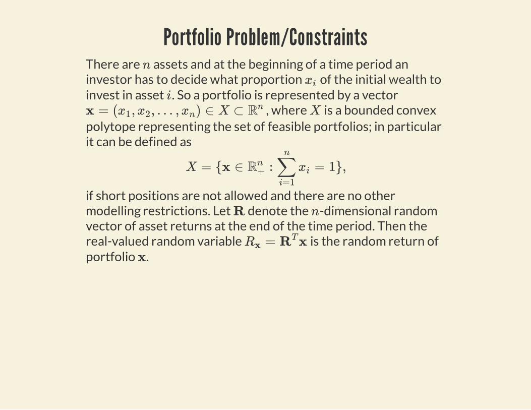
Portfolio Problem/ConstraintsThere are assets and at the beginning of a time period aninvestor has to decide what proportion of the initial wealth toinvest in asset . So a portfolio is represented by a vector

, where is a bounded convexpolytope representing the set of feasible portfolios; in particularit can be defined as

if short positions are not allowed and there are no othermodelling restrictions. Let denote the -dimensional randomvector of asset returns at the end of the time period. Then thereal-valued random variable is the random return ofportfolio .

nxi

ix = ( , , … , ) ∈ X ⊂x1 x2 xn Rn X

X = {x ∈ : = 1},Rn+ ∑

i=1

n

xi

R n

= xRx RT

x

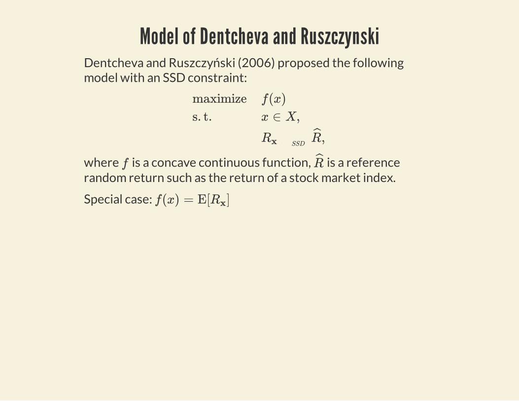
Model of Dentcheva and RuszczynskiDentcheva and Ruszczyński (2006) proposed the followingmodel with an SSD constraint:

where is a concave continuous function, is a referencerandom return such as the return of a stock market index.

Special case:

maximizes. t.

f(x)x ∈ X,

,Rx ?SSD

R

f R

f(x) = E[ ]Rx

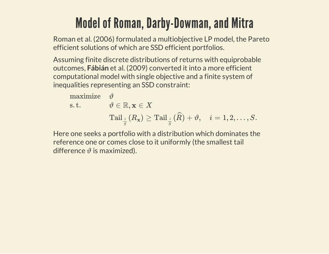
Model of Roman, Darby-Dowman, and MitraRoman et al. (2006) formulated a multiobjective LP model, the Paretoefficient solutions of which are SSD efficient portfolios.

Assuming finite discrete distributions of returns with equiprobableoutcomes, Fábián et al. (2009) converted it into a more efficientcomputational model with single objective and a finite system ofinequalities representing an SSD constraint:

Here one seeks a portfolio with a distribution which dominates thereference one or comes close to it uniformly (the smallest taildifference is maximized).

maximizes. t.

ϑ

ϑ ∈ R, x ∈ X

( ) ≥ ( ) + ϑ, i = 1, 2, … , S.Tail i

S

Rx Tail i

S

R

ϑ

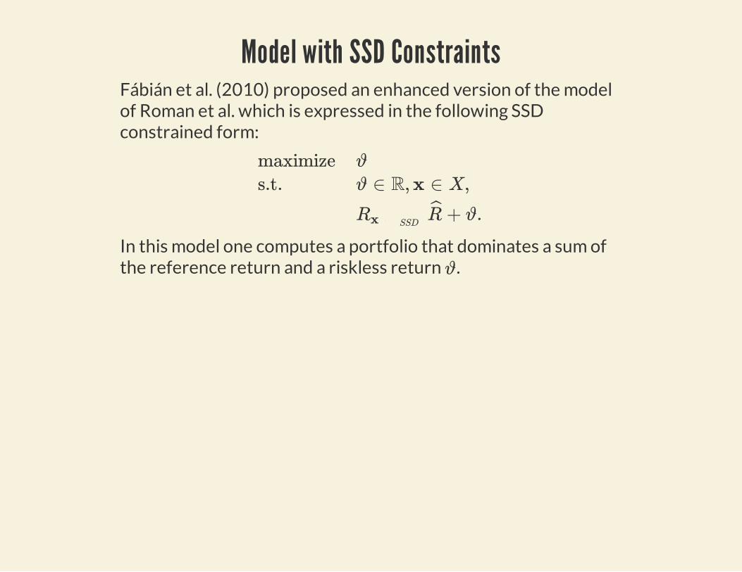
Model with SSD ConstraintsFábián et al. (2010) proposed an enhanced version of the modelof Roman et al. which is expressed in the following SSDconstrained form:

In this model one computes a portfolio that dominates a sum ofthe reference return and a riskless return .

maximizes.t.

ϑ

ϑ ∈ R, x ∈ X,

+ ϑ.Rx ?SSD

R

ϑ

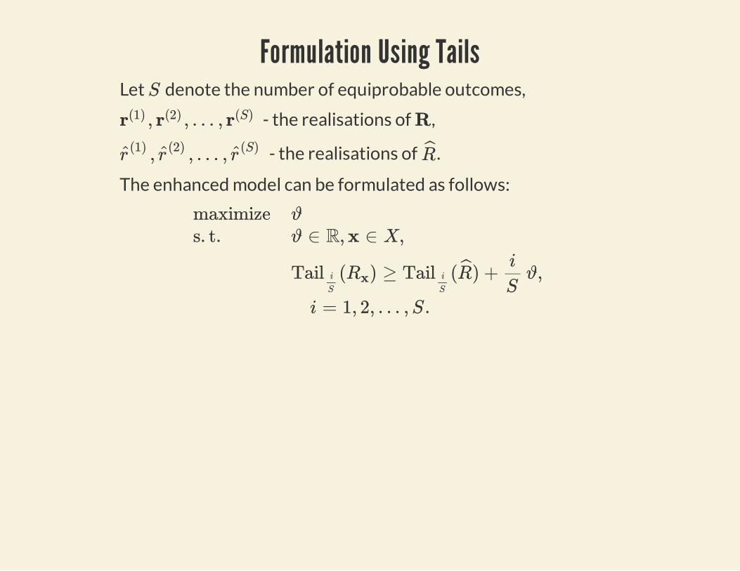
Formulation Using TailsLet denote the number of equiprobable outcomes,

- the realisations of ,

- the realisations of .

The enhanced model can be formulated as follows:

S

, , … ,r(1) r(2) r(S) R

, , … ,r(1)

r(2)

r(S)

R

maximizes. t.

ϑ

ϑ ∈ R, x ∈ X,

( ) ≥ ( ) + ϑ,Tail i

S

Rx Tail i

S

Ri

Si = 1, 2, … , S.

Cutting-Plane Formulation Using TailsFábián et al. (2009) obtained the cutting-plane representation of the

function:

Cutting-plane representation of the enhanced model:

where .

Tail

( ) =Tail i

S

Rx min x1S

∑j∈Ji

r(j)T

such that ⊂ {1, 2, … , S}, | | = i.Ji Ji

maximizes.t.

ϑϑ ∈ R, x ∈ X,

x ≥ + ϑ,1S

∑j∈Ji

r(j)T τii

S∀ ⊂ {1, 2, … , S},Ji

| | = i, i = 1, 2, … , S,Ji

= ( )τ i Tail i

S

R

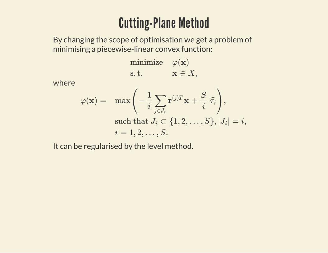
Cutting-Plane MethodBy changing the scope of optimisation we get a problem ofminimising a piecewise-linear convex function:

where

It can be regularised by the level method.

minimizes. t.

φ(x)x ∈ X,

φ(x) = max − x + ,⎛⎝ 1

i∑j∈Ji

r(j)T S

iτi

⎞⎠such that ⊂ {1, 2, … , S}, | | = i,Ji Ji

i = 1, 2, … , S.

Cut GenerationThe cut at the iteration is constructed as follows:

Let denote the solution of the approximation function atiteration and denote the orderedrealisations of .

Select Then

Sets correspond to ordered realisations.

l(x) k

∈ Xx∗

k ≤ ≤ … ≤r( )j∗1 r( )j∗

2 r( )j∗S

Rx∗

∈ − + .i∗ argmax1≤i≤S

⎛⎝ 1

i∑j∈J ∗

i

r(j)T x∗ S

iτ i

⎞⎠

l(x) = − x + .1i∗ ∑

j∈J ∗i∗

r(j)T S

i∗ τ i∗

= ( , … , )J ∗i j∗

1 j∗i

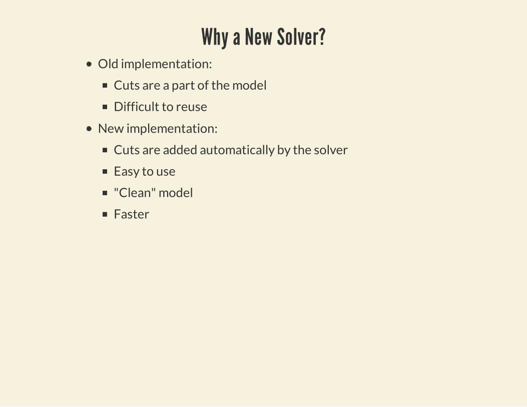
Why a New Solver?Old implementation:

Cuts are a part of the model

Difficult to reuse

New implementation:

Cuts are added automatically by the solver

Easy to use

"Clean" model

Faster

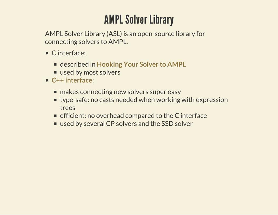
AMPL Solver LibraryAMPL Solver Library (ASL) is an open-source library forconnecting solvers to AMPL.

C interface:

described in Hooking Your Solver to AMPLused by most solvers

C++ interface:

makes connecting new solvers super easytype-safe: no casts needed when working with expressiontreesefficient: no overhead compared to the C interfaceused by several CP solvers and the SSD solver

SSD Solver ArchitectureSSD Solver

ASLExternalSolver

SSD SolverLibrary

SSD FunctionLibrary

AMPLproblem,options

solution

ASL does all the heavy lifting such as interaction with AMPLand an external solver which makes SSD solver implemenationvery simple (~300 LOC!)

Function library provides the ssd_uniform function that istranslated into an SSD relation by the solver.

External solver is used for subproblems.

Solver library is optional but facilitates testing.

Expression TreesThe solver extracts linear expressions from the expression treesrepresenting arguments of ssd_uniform.

LogicalExpr

CallExpr

NumberOfExpr

Variable

NumericConstant

PiecewiseLinearTerm

IfExpr

CountExpr

SumExpr

VarArgExpr (min, max)

BinaryExpr (+, ­, *, /, div, less, ...)

UnaryExpr (unary ­, abs, tan, ...)

NumericExprExpr

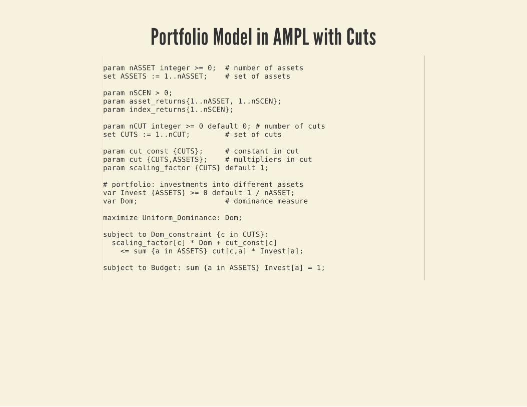
Portfolio Model in AMPL with Cutsparam nASSET integer >= 0; # number of assetsset ASSETS := 1..nASSET; # set of assets

param nSCEN > 0;param asset_returns{1..nASSET, 1..nSCEN};param index_returns{1..nSCEN};

param nCUT integer >= 0 default 0; # number of cutsset CUTS := 1..nCUT; # set of cuts

param cut_const {CUTS}; # constant in cutparam cut {CUTS,ASSETS}; # multipliers in cutparam scaling_factor {CUTS} default 1;

# portfolio: investments into different assetsvar Invest {ASSETS} >= 0 default 1 / nASSET;var Dom; # dominance measure

maximize Uniform_Dominance: Dom;

subject to Dom_constraint {c in CUTS}: scaling_factor[c] * Dom + cut_const[c] <= sum {a in ASSETS} cut[c,a] * Invest[a];

subject to Budget: sum {a in ASSETS} Invest[a] = 1;

Portfolio Model in AMPL using SSD Solverinclude ssd.ampl;

param NumScenarios;param NumAssets;

set Scenarios = 1..NumScenarios;set Assets = 1..NumAssets;

# Return of asset a in senario s.param Returns{a in Assets, s in Scenarios};

# Reference return in scenario s.param Reference{s in Scenarios};

# Fraction of the budget to invest in asset a.var invest{a in Assets} >= 0 <= 1;

subject to ssd_constraint{s in Scenarios}: ssd_uniform(sum{a in Assets} Returns[a, s] * invest[a], Reference[s]);

subject to budget: sum{a in Assets} invest[a] = 1;

Reference Returns

Performance

100 scenario problem with FTSE100 used as a reference.

The new implementation is 2-3 times faster.

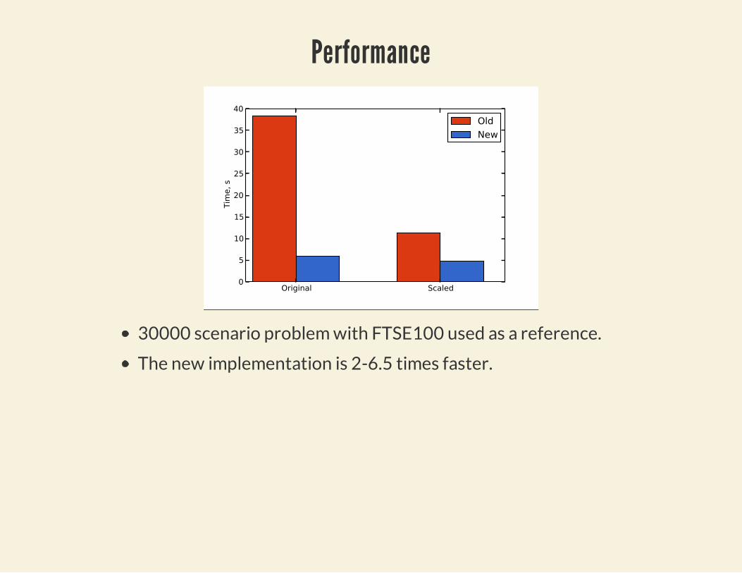
Performance

30000 scenario problem with FTSE100 used as a reference.

The new implementation is 2-6.5 times faster.

SummaryAMPL solver interface and ASL make implementation of high-level solvers/algorithms that use other solvers easy. The sametechnique can be applied to

other-cutting plane methods

decomposition methods, e.g. Bender's decomposition

New solver provides an efficient implementation of a cutting-plane algorithm for solving problems with SSD constraints.

This is in line with our approach that different types ofoptimisation models are matched with corresponding solvers.

ReferencesDentcheva, D. and Ruszczyński, A. (2006). Portfolio optimization with stochastic

dominance constraints. Journal of Banking & Finance, 30 , 433–451.

Fábián, C. I., Mitra, G., and Roman, D. (2009). Processing second-order stochastic

dominance models using cutting-plane representations. Mathematical Programming,

Series A. DOI: 10.1007/s10107-009-0326-1.

Fábián, C. I., Mitra, G., Roman, D., and Zverovich, V. (2010). An enhanced model for

portfolio choice with ssd criteria: a constructive approach. Quantitative Finance.

First published on: 11 May 2010.

Fishburn, P. C. and Vickson, R. G. (1978). Theoretical foundations of stochastic

dominance. In Stochastic Dominance: An Approach to Decision-Making Under Risk,

(pp. 37–113). D.C. Heath and Company, Lexington, Massachusetts.

Roman, D., Darby-Dowman, K., and Mitra, G. (2006). Portfolio construction based on

stochastic dominance and target return distributions. Mathematical Programming,

eries B, 108, 541–569.

Thank you! AMPL Optimization