A solution to the random assignment problem on the full

preference domain∗

Akshay-Kumar Katta† Jay Sethuraman ‡

January 2004; Revised February 2005

Abstract

We consider the problem of allocating a set of indivisible objects to agents in a fair and

efficient manner. In a recent paper, Bogomolnaia and Moulin consider the case in which all

agents have strict preferences, and propose the probabilistic serial (PS) mechanism; they

define a new notion of efficiency, called ordinal efficiency, and prove that the probabilistic

serial mechanism finds an envy-free ordinally efficient assignment. However, the restrictive

assumption of strict preferences is critical to their algorithm. Our main contribution is

an analogous algorithm for the full preference domain in which agents are allowed to be

indifferent between objects. Our algorithm is based on a reinterpretation of the PS mech-

anism as an iterative algorithm to compute a “flow” in an associated network. In addition

we show that on the full preference domain it is impossible for even a weak strategyproof

mechanism to find a random assignment that is both ordinally efficient and envy-free.

∗This research was supported by an NSF grant DMI-0093981 and an IBM partnership award.†Department of Industrial Engineering and Operations Research, Columbia University, New York, NY; email:

ark2001@columbia.edu‡Department of Industrial Engineering and Operations Research, Columbia University, New York, NY; email:

jay@ieor.columbia.edu

1

1 Introduction

The problem of allocating a number of indivisible objects to a number of agents, each desiring

at most one object, in a fair and efficient manner is fundamental in many applications. If

only one indivisible object must be allocated to n > 1 agents, there is really only one fair and

efficient solution1: assigning the object to an agent chosen uniformly at random among the

n agents. When there are many objects the problem becomes substantially more interesting

for a number of reasons: (i) many definitions of fairness and efficiency are possible; (ii) richer

mechanisms emerge; and (iii) since preferences of the agents over the objects have to be solicited

from the agents, truthfulness of the allocation mechanism becomes important.

A natural approach to the problem of allocating multiple objects among many agents is

to generalize the simple “lottery” mechanism: order the agents uniformly at random and let

them successively choose an available object according to this (random) order; thus the first

agent picks his favorite object, the second agent picks his favorite object among the remaining

objects, etc. This is the random priority mechanism, and has a number of attractive features:

it is ex post efficient and truthful (or strategyproof: revealing true preferences is a dominant

strategy for all the agents); it is fair in the weak sense of equal treatment of equals (agents with

identical preferences are treated in an identical manner, a priori); however, it is not efficient

when agents are endowed with utility functions consistent with their preferences, that is, it is

not ex ante efficient. Moreover, it is not fair in the stronger sense of envy-freeness (described

later).

A second solution to this problem adapts the competitive equilibrium with equal incomes

(CEEI) solution for the fair division of unproduced commodities. This solution is envy-free

and ex ante efficient, but is not strategyproof. Moreover, the computational and informational

requirements of implementing this mechanism are prohibitive: it requires the solution of a

fixed-point problem, and requires a complete knowledge of the utility functions of the agents.

In contrast, the random priority mechanism is very simple to implement, and only requires the

agents to report their “preferences” over objects.

Our work is inspired by the remarkable paper of Bogomolnaia and Moulin [5], who proposed

a new mechanism (PS) for the random assignment problem. Their mechanism combines the

attractive features of the random priority mechanism and the CEEI solution: it requires the

agents to report their preferences over objects, not the complete utility functions, and yet

computes a random assignment that is ordinally efficient and envy-free. Ordinal efficiency is

stronger than ex post efficiency but weaker than ex ante efficiency; given the “ordinal” nature of

the input to the mechanism (only preference rankings are used, not complete utility functions),

this is perhaps the most meaningful notion of efficiency for an ordinal mechanism. Finally, the

mechanism proposed by Bogomolnaia and Moulin is not truthful, it satisfies a weaker version

of that property.

Unfortunately, the work of Bogomolnaia and Moulin [5] (and most of the existing work

on this problem so far) assumes that all preferences are strict, which is a fairly restrictive

1We assume that monetary compensations are not allowed.

2

requirement in many practical settings. A natural question then is to ask if these results have

analogs in the more general case of a full preference domain. As discussed by Bogomolnaia, Deb,

and Ehlers [4], there are both practical and technical reasons for studying the full preference

domain. Moreover, it has generally been recognized that the natural preference domain for

many allocation problems in economic settings is the full preference domain.

Contributions. Our main contribution in this paper is a solution to the random assignment

problem in which indifferences are permitted. The solution we propose can be viewed as a

natural extension of the PS mechanism to the full domain. Our proposed solution is ordinally

efficient and envy-free. Furthermore we show that for this richer preference domain, it is

not possible for any mechanism to find an envy-free, ordinally efficient assignment and still

satisfy the weaker version of strategyproofness satisfied by the PS mechanism in the strict

preference domain. This observation indeed reveals that the full preference domain is subtler

and fundamentally different from the strict preference domain for the problems studied here.

Our techniques rely on standard tools from network flow theory: the mechanism we propose

can be viewed as an iterative application of an algorithm to compute the maximum flow in a

parametric network. We first consider an extreme special case in which each agent partitions

the available objects into acceptable and unacceptable objects, but is indifferent between the

objects in each of these classes. Our algorithm for the full preference domain is an iterative

application of the algorithm for this special case. This special case is an interesting problem in

its own right and has been independently studied by Bogomolnaia and Moulin [7] recently. We

show that the algorithm proposed for this special case is identical to an algorithm to compute

a lexicographically optimal flow in a network; this establishes a connection to the sharing

problem and its variants, which have been studied by operations researchers.

The remainder of this paper is organized as follows. In §2 we describe the problem, define

various notions of fairness and efficiency, and describe the notation. A description of relevant

past work appears in §3 followed by the impossibility result in §4. We consider the special

case of two indifference classes in §5, and provide an algorithm to solve it by posing it as a

parametric maximum flow problem. This algorithm serves as the basis for the main result,

described in §6, which also contains a characterization of ordinally efficient assignments as well

as a method to compute them.

2 Problem Description and Definitions

Problem Description. We consider the problem of allocating indivisible objects to agents

so that each agent receives at most one object. Agents have preferences over the objects, and

the allocation mechanism takes this profile of preferences as input. The preference ordering of

each agent is assumed to be transitive and complete (every pair of objects is comparable). Thus,

given a pair of objects, an agent strictly prefers one to the other or is indifferent between them;

both the indifference relation and the strict preference relation are transitive. The preference

ordering of agent i is denoted by ≥i, with >i and =i denoting the strict preference relation and

3

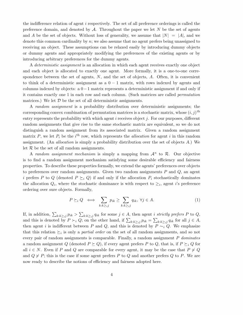
the indifference relation of agent i respectively. The set of all preference orderings is called the

preference domain, and denoted by A. Throughout the paper we let N be the set of agents

and A be the set of objects. Without loss of generality, we assume that |N | = |A|, and we

denote this common cardinality by n; we also assume that no agent prefers being unassigned to

receiving an object. These assumptions can be relaxed easily by introducing dummy objects

or dummy agents and appropriately modifying the preferences of the existing agents or by

introducing arbitrary preferences for the dummy agents.

A deterministic assignment is an allocation in which each agent receives exactly one object

and each object is allocated to exactly one agent. More formally, it is a one-to-one corre-

spondence between the set of agents, N , and the set of objects, A. Often, it is convenient

to think of a deterministic assignment as a 0 − 1 matrix, with rows indexed by agents and

columns indexed by objects: a 0−1 matrix represents a deterministic assignment if and only if

it contains exactly one 1 in each row and each column. (Such matrices are called permutation

matrices.) We let D be the set of all deterministic assignments.

A random assignment is a probability distribution over deterministic assignments; the

corresponding convex combination of permutation matrices is a stochastic matrix, whose (i, j)th

entry represents the probability with which agent i receives object j. For our purposes, different

random assignments that give rise to the same stochastic matrix are equivalent, so we do not

distinguish a random assignment from its associated matrix. Given a random assignment

matrix P , we let Pi be the ith row, which represents the allocation for agent i in this random

assignment. (An allocation is simply a probability distribution over the set of objects A.) We

let R be the set of all random assignments.

A random assignment mechanism is simply a mapping from An to R. Our objective

is to find a random assignment mechanism satisfying some desirable efficiency and fairness

properties. To describe these properties formally, we extend the agents’ preferences over objects

to preferences over random assignments. Given two random assignments P and Q, an agent

i prefers P to Q (denoted P �i Q) if and only if the allocation Pi stochastically dominates

the allocation Qi, where the stochastic dominance is with respect to ≥i, agent i’s preference

ordering over sure objects. Formally,

P �i Q ⇐⇒∑

k:k≥ij

pik ≥∑

k:k≥ij

qik, ∀j ∈ A. (1)

If, in addition,∑

k:k≥ijpik >

∑k:k≥ij

qik for some j ∈ A, then agent i strictly prefers P to Q,

and this is denoted by P �i Q; on the other hand, if∑

k:k≥ijpik =

∑k:k≥ij

qik for all j ∈ A,

then agent i is indifferent between P and Q, and this is denoted by P ∼i Q. We emphasize

that this relation �i is only a partial order on the set of all random assignments, and so not

every pair of random assignments is comparable. Finally, a random assignment P dominates

a random assignment Q (denoted P � Q), if every agent prefers P to Q, that is, if P �i Q for

all i ∈ N . Even if P and Q are comparable for every agent, it may be the case that P 6� Q

and Q 6� P ; this is the case if some agent prefers P to Q and another prefers Q to P . We are

now ready to describe the notions of efficiency and fairness adopted here.

4

Efficiency. A random assignment P is ordinally efficient if it is not dominated by any other

random assignment Q. If we apply this definition to a deterministic assignment—a random

assignment in which the entries are 0 or 1—then we recover the familiar definition of Pareto

efficiency. Thus, ordinal efficiency can be viewed as a natural extension of Pareto efficiency

to the random assignment setting. Other extensions are possible and have been considered in

the literature; we briefly discuss two such extensions, one weaker and one stronger. A random

assignment is ex post efficient if it can be represented as a probability distribution over Pareto

efficient deterministic assignments. A random assignment is ex ante efficient if for any profile

of utility functions consistent with the preference profile of the agents, the resulting expected

utility vector is Pareto efficient: for any random assignment in which the expected utility of

some agent is strictly greater, there must be another agent whose expected utility is strictly

lower. It is easy to show that ex ante efficiency implies ordinal efficiency, which implies ex

post efficiency. The relationship between the various notions of efficiency are explored further

by Abdulkadiroglu and Sonmez [2] and McLennan [17]. The attractive feature of ordinal

efficiency is that its informational requirements are low: it relies only on agents’ preferences

over objects, not on their preferences over random allocations; yet, it is stronger than ex post

efficiency (which also only requires preferences over objects). For this reason we shall restrict

ourselves to ordinally efficient assignments in the rest of this paper.

Fairness. A random assignment P is envy-free if each agent prefers her allocation to that

of any other agent. Formally, P is envy-free if Pi �i Pi′ for all i, i′ ∈ N . A weaker version of

envy-freeness can also be defined: P is weakly envy-free if no agent strictly prefers someone

else’s allocation to hers, that is, if Pi′ 6�i Pi for all i, i′ ∈ N . A random assignment P satisfies

equal treatment of equals if agents with identical preferences get identical allocations (Pi = Pi′

if ≥i≡≥i′). Another notion of fairness is anonymity: a random assignment mechanism is

anonymous if its outcome depends only on the profile of preferences and does not depend on

the identity of the agents. Most of the mechanisms we consider will be anonymous mechanisms.

Again, it is easy to show that envy-freeness implies weak envy-freeness and equal treatment

of equals. (It is easy to see that weak envy-freeness and equal treatment of equals are not

comparable: it is easy to construct assignments that satisfy one property but not the other.)

In most of this paper, we shall restrict ourselves to envy-free assignments.

Incentives. A random assignment mechanism is said to be strategyproof if revealing the

true preference ordering is a dominant strategy for each agent. Again a weaker notion of

strategyproofness can be defined: A mechanism is weakly strategyproof if by falsifying her

preference list an agent cannot obtain an allocation that she strictly prefers to her true alloca-

tion. A mechanism is group strategyproof if it is not possible for any coalition S to improve its

allocation (meaning, each agent in S is atleast as well off, and at least one of them is strictly

better off) by falsifying their preferences.

5

3 Related Work

Strict Preferences. Several solutions have been proposed to the random assignment prob-

lem. The earliest work on this problem is due to Hylland and Zeckhauser [14], who adapt the

competitive equilibrium with equal incomes (CEEI) solution. The mechanism is “expensive”

both in terms of its informational requirements (needs utility functions of all individuals) and

in terms of its computational requirements (requires the solution of a fixed-point problem).

The resulting solution is envy-free and Pareto efficient with respect to the utility functions,

but the mechanism is not strategyproof. Gale [10] conjectured that this is the best possible,

specifically, that no strategyproof mechanism that elicits utility functions and achieves Pareto

efficiency with respect to these utility functions can find a “fair” solution, even in the weaker

sense of equal treatment of equals. This conjecture was proved by Zhou [26].

The prohibitive cost of CEEI motivated research on finding simpler mechanisms. A natural

candidate was the random priority (RP) mechanism: order the agents uniformly at random,

and let them successively choose an object in that order. This was analyzed by Abdulkadiroglu

and Sonmez [1] who showed that RP is equivalent to the unique core allocation of the Shapley-

Scarf housing market [23] in which each agent is endowed with an object chosen uniformly at

random; Roth and Postlewaite [22] had earlier shown that any Shapley-Scarf housing market

with strict preferences has a unique core, and Roth [21] proved that the core (from random

endowments) is strategyproof, anonymous (does not depend on the labels of the agents), and

ex-post Pareto efficient. The equivalence of RP with the core from random endowments implies

that RP itself is strategyproof, anonymous, and always an ex-post Pareto efficient solution; in

fact, Abdulkadiroglu and Sonmez showed [1] that the only Pareto efficient matching mecha-

nisms are serial dictatorships, which are like RP, except that the initial ordering of the agents

is chosen in a deterministic fashion. Svensson [25] showed that serial dictatorships are the only

rules satisfying satisfying strategyproofness, neutrality and nonbossiness. Zhou [26] showed that

the solution computed by RP may not be efficient if agents are endowed with utility functions

consistent with their preferences.

Bogomolnaia and Moulin [5] considered mechanisms that combined the “best” of CEEI

and RP: the CEEI solution has strong efficiency and fairness properties, but is not strate-

gyproof; the RP solution is strategyproof but has weaker efficiency and fairness properties.

The key contribution of Bogomolnaia and Moulin [5] is the definition of an intermediate no-

tion of efficiency—ordinal efficiency–and natural mechanisms to find all ordinally efficient solu-

tions. They also showed that one such mechanism—the probabilistic serial (PS) mechanism—is

weakly strategyproof, and achieves an envy-free, ordinally efficient solution. In a result parallel

to Zhou’s impossibility theorem, they show that no strategyproof mechanism can achieve both

ordinal efficiency and fairness, even in the weak sense of equal treatment of equals. All of their

results were derived in the setting of a strict preference domain; the extension to the “full

domain” (that allows for “subjective indifferences”) was left as a challenging open problem at

the end of their work, and is addressed here.

The PS mechanism was introduced by Cres and Moulin [9] in the context of a scheduling

6

problem with opting out. In that model, every agent has a job that needs unit time on a

machine by a certain deadline; thus the objects are really possible time-slots to which jobs can

be assigned. Agents have strictly decreasing, positive, utilities for the time-slots to which their

jobs can be feasibly assigned, and a utility of zero for not being assigned a time-slot before their

deadline. (Thus agents’ preference orderings are identical; only their deadlines and utilities may

vary.) Cres and Moulin [9] show that in their model the PS solution stochastically dominates

the RP solution. Bogomolnaia and Moulin [6] introduced the concept of ordinal efficiency in

that model and provided two different characterizations of the PS mechanism: it is the only

mechanism that is ordinally efficient, strategyproof, and satisfies equal treatment of equals;

and it is the only mechanism that is ordinally efficient and envy-free.

Full domain. As mentioned earlier, most of the work dealing with the assignment problem

is in the setting of the strict preference domain. Important exceptions include the work of

Svensson [24] and the recent work of Bogomolnaia et al. [4]. Svensson [24] introduces a

class of rules—Serially Dictatorial Rules—that satisfy a number of desirable properties like ef-

ficiency, neutrality, and strategyproofness. This class of rules was generalized by Bogomolnaia

et al. [4] to the class of Bi-Polar Serially Dictatorial Rules, who, more importantly, charac-

terized these rules by essential single-valuedness, nonbossiness, strategyproofness, and Pareto

indifference. Further, they show that an assignment rule satisfies single-valuedness, efficiency,

strategyproofness and weak non-bossiness if and only if it is a selection from a Bi-Polar Seri-

ally Dictatorial Rule. They compare and contrast these rules to allocation rules arising from

traditional exchange-based approaches, and also include an illuminating discussion of the dif-

ficulties and surprises one encounters when studying the full preference domain. In particular,

they show that results that hold for the full preference domain may not hold for the strict

preference domain, and vice-versa. While these two papers study the full preference domain,

they consider only deterministic mechanisms, and so cannot deal with fairness issues. (Recall

that monetary compensations are not permitted.) In contrast, we are concerned with finding

a random assignment that is efficient and envy-free.

4 An Impossibility Result

Our first result establishes that on the full preference domain, ordinal efficiency and envy-

freeness are incompatible with strategyproofness even in the weak sense. This is in contrast to

the result of Bogomolnaia and Moulin [5], who showed that on the strict preference domain,

the PS mechanism is weakly strategyproof and finds an envy-free, ordinally efficient solution.

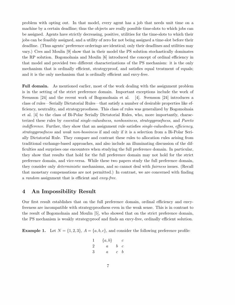
Example 1. Let N = {1, 2, 3}, A = {a, b, c}, and consider the following preference profile:

1 {a, b} c

2 a b c

3 a c b

7

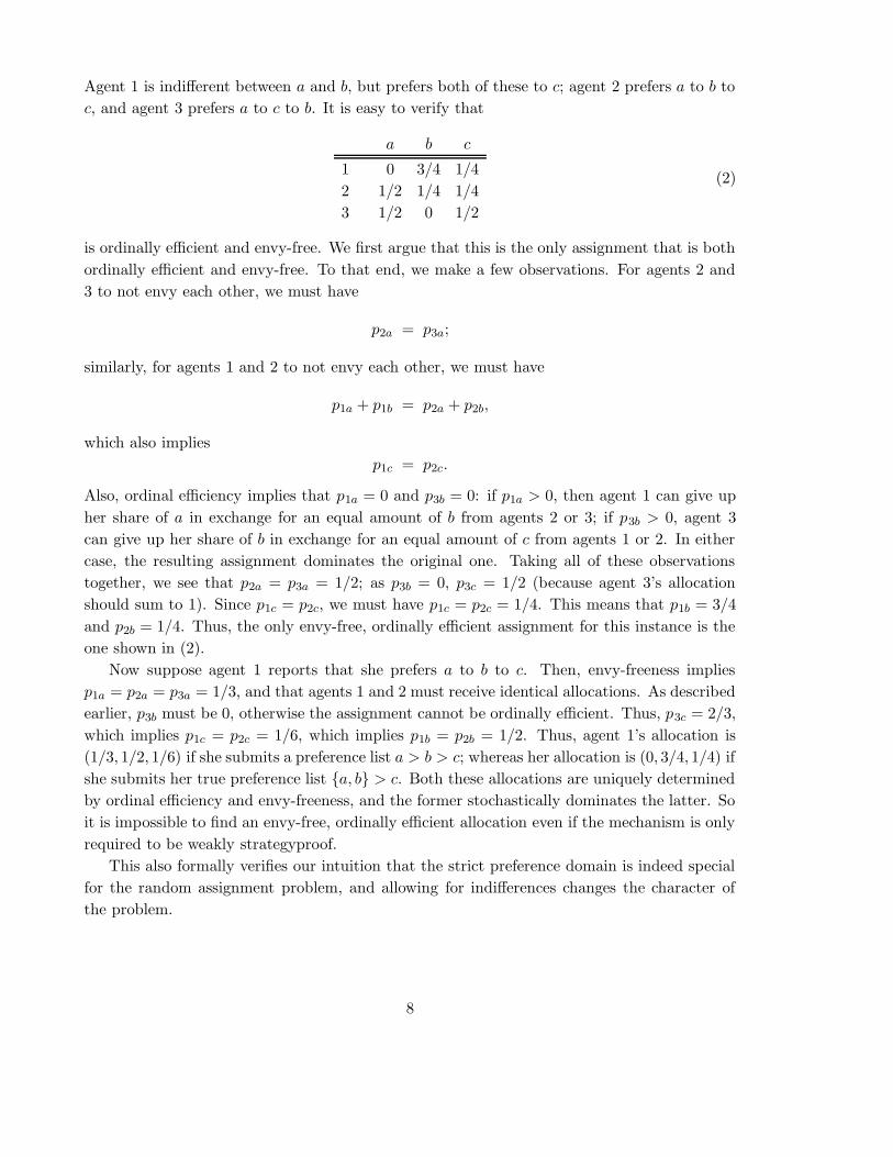
Agent 1 is indifferent between a and b, but prefers both of these to c; agent 2 prefers a to b to

c, and agent 3 prefers a to c to b. It is easy to verify that

a b c

1 0 3/4 1/4

2 1/2 1/4 1/4

3 1/2 0 1/2

(2)

is ordinally efficient and envy-free. We first argue that this is the only assignment that is both

ordinally efficient and envy-free. To that end, we make a few observations. For agents 2 and

3 to not envy each other, we must have

p2a = p3a;

similarly, for agents 1 and 2 to not envy each other, we must have

p1a + p1b = p2a + p2b,

which also implies

p1c = p2c.

Also, ordinal efficiency implies that p1a = 0 and p3b = 0: if p1a > 0, then agent 1 can give up

her share of a in exchange for an equal amount of b from agents 2 or 3; if p3b > 0, agent 3

can give up her share of b in exchange for an equal amount of c from agents 1 or 2. In either

case, the resulting assignment dominates the original one. Taking all of these observations

together, we see that p2a = p3a = 1/2; as p3b = 0, p3c = 1/2 (because agent 3’s allocation

should sum to 1). Since p1c = p2c, we must have p1c = p2c = 1/4. This means that p1b = 3/4

and p2b = 1/4. Thus, the only envy-free, ordinally efficient assignment for this instance is the

one shown in (2).

Now suppose agent 1 reports that she prefers a to b to c. Then, envy-freeness implies

p1a = p2a = p3a = 1/3, and that agents 1 and 2 must receive identical allocations. As described

earlier, p3b must be 0, otherwise the assignment cannot be ordinally efficient. Thus, p3c = 2/3,

which implies p1c = p2c = 1/6, which implies p1b = p2b = 1/2. Thus, agent 1’s allocation is

(1/3, 1/2, 1/6) if she submits a preference list a > b > c; whereas her allocation is (0, 3/4, 1/4) if

she submits her true preference list {a, b} > c. Both these allocations are uniquely determined

by ordinal efficiency and envy-freeness, and the former stochastically dominates the latter. So

it is impossible to find an envy-free, ordinally efficient allocation even if the mechanism is only

required to be weakly strategyproof.

This also formally verifies our intuition that the strict preference domain is indeed special

for the random assignment problem, and allowing for indifferences changes the character of

the problem.

8

5 Random Assignment with Dichotomous Preferences

In designing a mechanism for the random assignment problem on the full preference domain,

it seems natural to first understand some extreme special cases. The case of no indifferences

(i.e., strict preferences) is one extreme; the case of dichotomous preferences, discussed in this

section, is the other. Specifically, we assume that each agent partitions the set of objects into

two classes: the set of acceptable objects, and the set of unacceptable objects. Three reasons

underlie our focus on this special case: first, our solution to the overall problem is essentially an

iterative application of the ideas that help solve this special case; second, stronger results can

be proved for this special case, which may be of independent interest; and third, the algorithm

used to solve this special case is identical to the algorithm for finding a lexicographically optimal

(lex-opt) flow in a network, first discovered by Megiddo [19]. We note that, independently of

our work, Bogomolnaia and Moulin [7] have studied the same problem, using somewhat similar

methods, and have obtained the same results. In particular, the impossibility result of §4 does

not hold, and in fact, the proposed mechanism is group strategyproof and finds an ordinally

efficient, envy-free assignment. All the results of this section were originally proved in [7], so

we simply state them without detailed proofs. However, we describe the mechanism in detail

because our point of view is algorithmic, whereas the description in [7] is structural. Our main

contribution in this section is simply the observation that the random assignment problem with

dichotomous preferences is closely related to a classical “sharing” problem considered earlier

in the operations research literature. We briefly discuss this relationship at the end of this

section.

In an instance of the random assignment problem with dichotomous preferences, each agent

indicates only the subset of objects that she finds acceptable, each of which gives her unit

utility; the other objects are unacceptable, yielding zero utility. We assume that each agent

finds at least one object acceptable; agents who do not meet this assumption are irrelevant

to the problem as they will necessarily have zero utility in all solutions. Let Li ⊆ A be the

set of all acceptable objects for agent i; recall that she is indifferent between any two objects

in Li. Thus, for a random assignment P , the utility (or welfare-level) ui of agent i is simply∑j:j∈Li

pij, the probability that she is assigned an acceptable object.

Remark. Note that the random assignment problem with dichotomous preferences can be

solved by adapting the random priority algorithm as well; we do not describe this adaptation

because (a) the results for the natural adaptation of the random priority mechanism are weaker;

and (b) our goal is to use this mechanism to eventually find an ordinally efficient assignment

on the full preference domain, and we know from Bogomolnaia and Moulin [5] that the random

priority mechanism does not find an ordinally efficient assignment.

5.1 Algorithm and Analysis

Overview. Suppose the preference profile in a given instance of the random assignment

problem is such that some set of three agents have only two acceptable objects among them.

9

Then, it is obvious that the combined utilities of these three agents cannot exceed 2. The

general algorithm for solving the problem builds on this trivial observation: it consists of

locating such a “bottleneck” subset of agents, and allocating their acceptable objects amongst

them in a “fair” way, eliminating these agents and their acceptable objects, and recursively

applying the idea on the remaining set of agents and objects. To formalize this, let Γ(Y )

denote the set of objects acceptable to at least one agent in Y , for any Y ⊆ N , and let

v = minY ⊆N

|Γ(Y )|

|Y |,

with X denoting the largest cardinality set Y ⊆ N with |Γ(Y )|/|Y | = v. If v ≥ 1, there are

more objects than agents competing for it, so each agent can be assigned a distinct object,

and there is nothing more to do. If v < 1, the algorithm allocates the objects in Γ(X) among

the agents in X such that the utility of any agent i ∈ X is exactly v; such an assignment

would completely use up the objects in Γ(X), so none of these objects can even be fractionally

assigned to the other agents; moreover, the agents in X cannot be assigned any other object.

Thus, the agents in X and the objects in Γ(X) can be removed from the problem as they play

no further role. The same calculations are carried out in the residual problem with agents

N \ X, objects A \ Γ(X), and the preference profiles of the agents restricted to the these

“currently available” objects. Note that this is exactly the algorithm proposed in [7].

The only remaining details are the identification of the “bottleneck” subset X of agents,

and the precise allocation of the “bottleneck” set of objects, Γ(X), to the agents in X. It is

an elementary exercise to show both of these problems can be solved simultaneously as the

problem of finding a maximum flow in an appropriately defined network. We provide the

argument for the sake of completeness.

Flows and cuts. Network flow models arise naturally in the design and analysis of

communication, logistics, and transportation networks, as well as in many other contexts.

These models are among the best-understood and most used optimization models in practice.

(For background on network flow problems and techniques, we recommend [3].)

A directed graph G = (V,A) consists of a set of nodes V and a set of directed arcs A, which

are simply ordered pairs of distinct nodes. We will use the terms arcs and edges interchangeably.

A network is simply a directed graph with some additional data associated with the nodes and

arcs such as capacities and costs. We can view the nodes of a network as representing demand

or supply points of a commodity that is transported via the arcs. Given any network with a

source node s ∈ V , a sink node t ∈ V , and capacities uij on arc (i, j) ∈ A, the maximum flow

problem is to find the maximum amount of flow that can be sent from s to t without exceeding

arc capacities. A classical result in network flow theory connects the maximum flow problem

to a related problem called the minimum cut problem. Before describing this result, we need

to define the notion of a cut and its capacity.

Cut : A cut is any partition of V into S and S̄ := V \ S such that s ∈ S and t ∈ S̄; it is

sometimes called an s − t cut. Since S̄ = V \ S, we often refer to the cut simply by S instead

of the pair (S, S̄).

10

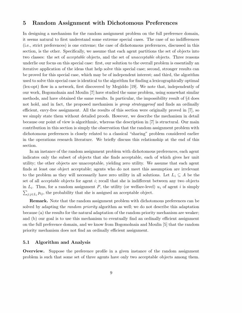
Figure 1: A network

Capacity of a cut: The capacity of the cut (S, S̄) is the sum of the capacities of all the arcs

that are directed from a node in S to a node in S̄ (i.e.∑

(i,j)∈A:i∈S,j∈S̄ uij).

Obviously, the maximum flow from s to t can be no more than the capacity of any s − t

cut; in particular, the maximum flow from s to t is at most the minimum capacity s − t cut.

The max-flow min-cut theorem asserts that the maximum s − t flow is equal to the capacity

of minimum s − t cut. This is a classical result in network flow theory, and can be proved

easily from linear programming duality. Hence, to show that a given flow on a network is

optimal, it is enough to demonstrate that there is a cut in the network with the same capacity

as the value of the flow. For example, consider the network shown in Figure 1, where the

label uij , fij on arc (i, j) indicates its capacity and current flow respectively. The value of the

flow in the network ( i.e the amount of flow out of s or into t ) is 15. Now consider the cut

(S, S̄) where S = {s, 1} and S̄ = {2, t}. The set of arcs which go from a node in S into a

node in S̄ is {((s, 2), (1, 2), (1, t)} and hence the capacity of this cut is 6+1+8=15. Therefore,

we can conclude that the given flow is a maximum flow. The relevance to the problem under

consideration should be clear by now: we plan to identify the bottleneck subset as an s− t cut

in a suitably defined graph; the precise manner by which the bottleneck objects are distributed

among the bottleneck agents will be given by a maximum s − t flow.

Consider the bipartite graph with nodes corresponding to N and A, and directed edges

(i, j) for i ∈ N, j ∈ Li. Let these edges have infinite capacity. Augment the network by adding

a source node s, a sink node t; edges with capacity λ ≥ 0 going from s to each node in N ,

and edges with unit capacity going from each node in A to t. Let V = N ∪ {s} ∪ {t} denote

the set of vertices in the augmented network. We view λ ≥ 0 as a parameter, and study the

minimum-capacity s− t cuts (or simply minimum cuts) in the network as λ is varied. For the

problem under consideration, it is clear that λ will be varied only in the interval [0, 1]. Fix any

such λ, and consider any s− t cut (S, S̄). It is clear that S must be of the form s∪X ∪W for

some X ⊆ N and W ⊆ A. Furthermore since the “original” edges (i.e. those from the agents

to their acceptable objects) have infinite capacity, W ⊇ Γ(X) in any minimum cut (otherwise,

we will have an edge of infinite capacity in the cut). The capacity of such a cut is then

λ(|N | − |X|) + |W |,

11

which shows that W = Γ(X) in any minimum cut. Thus, any minimum cut (S, S̄) is completely

determined by the set X, and and is of the form S = s ∪ X ∪ Γ(X) with capacity

λ(|N | − |X|) + |Γ(X)|.

When several minimum cuts exist, we pick the minimum-cut with the largest |X|. (This is

unique.)

For λ sufficiently close to 0, it is clear that X = ∅ gives the minimum cut, whose capacity

grows linearly in λ. We consider two possibilities, depending on whether or not X = ∅ is a

minimum cut for λ = 1. If it is, it will be clear from the following argument that each agent can

be assigned an acceptable object with probability 1, and there is nothing more to do. If X = ∅

is not a minimum cut for λ = 1, let λ∗ ∈ (0, 1) be the smallest value of λ for which X = ∅ is

not the only minimum cut, that is, some set X with |X| > 0 is also a minimum cut. (By our

convention, X = ∅ could be a minimum cut, but is not the only one.) Let X ∗ be the minimum

cut for λ = λ∗. By definition, for any λ < λ∗, X = ∅ was the minimum-cut, with capacity

λ|N |. It is clear (by continuity) that the capacity of the minimum-cut for λ = λ∗ must be

exactly λ∗|N |; since X∗ is a minimum-cut for λ = λ∗ and has capacity λ∗(|N |−|X∗|)+|Γ(X∗)|,

we have

λ∗|N | = λ∗(|N | − |X∗|) + |Γ(X∗)|,

from which we get

λ∗ =|Γ(X∗)|

|X∗|. (3)

Let λ = λ∗, and consider any Y ⊆ N ; the capacity of the cut s ∪ Y ∪ Γ(Y ) is simply

λ∗(|N | − |Y |) + |Γ(Y )|, which must be at least as large as the minimum-cut capacity λ∗|N |.

This, combined with Eq. (3), establishes

λ∗ = minY ⊆N

|Γ(Y )|

|Y |; X∗ = arg min

Y ⊆N

|Γ(Y )|

|Y |.

By our convention, X∗ is the largest cardinality subset of agents with this property.

Consider the network with λ = λ∗. By the max-flow min-cut theorem, the maximum flow

from s to t in this network matches the capacity of the minimum cut, which equals λ∗|N |.

However, every edge from s has capacity exactly λ∗ (and there are exactly |N | such edges), so

all of these edges carry a flow of λ∗ in a maximum flow; in particular, λ∗ units reach the sink

from each i ∈ X∗, which gives us the required random assignment.

The quantity λ∗ is the (smallest) breakpoint of the min-cut capacity function of the para-

metric network. The breakpoints of the min-cut capacity function of a parametric network are

well-understood [11]. Efficient algorithms to compute these breakpoints have been discovered

by several researchers, see [3]; the fastest of these methods, discovered by Gallo, Grigoriadis

and Tarjan [11], is based on the preflow-push algorithm for the maximum flow problem due to

Goldberg and Tarjan [12]. Gallo et al. [11] propose algorithms to find maximum flows in an

n-node, m-arc network for O(n) values of the parameter in O(nm log(n2/m)) time. In addi-

tion, they study the min-cut capacity as a function of a parameter λ and propose algorithms

12

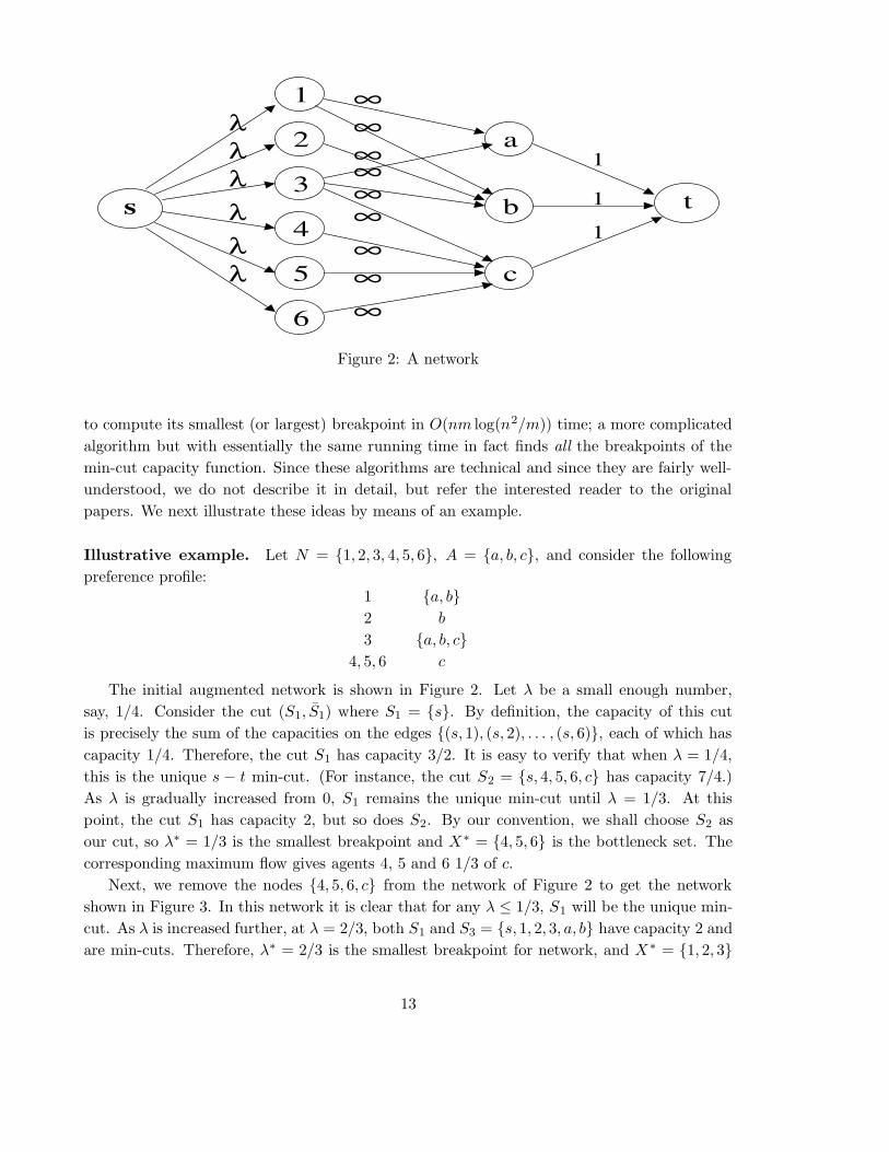
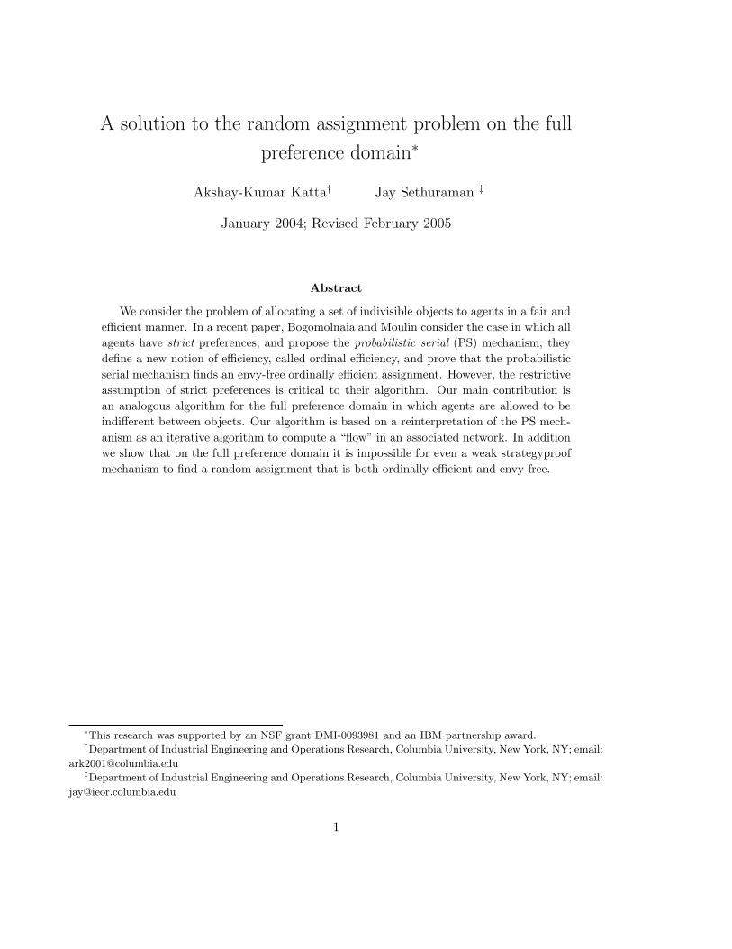
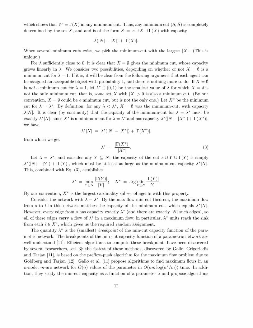
Figure 2: A network

to compute its smallest (or largest) breakpoint in O(nm log(n2/m)) time; a more complicated

algorithm but with essentially the same running time in fact finds all the breakpoints of the

min-cut capacity function. Since these algorithms are technical and since they are fairly well-

understood, we do not describe it in detail, but refer the interested reader to the original

papers. We next illustrate these ideas by means of an example.

Illustrative example. Let N = {1, 2, 3, 4, 5, 6}, A = {a, b, c}, and consider the following

preference profile:1 {a, b}

2 b

3 {a, b, c}

4, 5, 6 c

The initial augmented network is shown in Figure 2. Let λ be a small enough number,

say, 1/4. Consider the cut (S1, S̄1) where S1 = {s}. By definition, the capacity of this cut

is precisely the sum of the capacities on the edges {(s, 1), (s, 2), . . . , (s, 6)}, each of which has

capacity 1/4. Therefore, the cut S1 has capacity 3/2. It is easy to verify that when λ = 1/4,

this is the unique s − t min-cut. (For instance, the cut S2 = {s, 4, 5, 6, c} has capacity 7/4.)

As λ is gradually increased from 0, S1 remains the unique min-cut until λ = 1/3. At this

point, the cut S1 has capacity 2, but so does S2. By our convention, we shall choose S2 as

our cut, so λ∗ = 1/3 is the smallest breakpoint and X∗ = {4, 5, 6} is the bottleneck set. The

corresponding maximum flow gives agents 4, 5 and 6 1/3 of c.

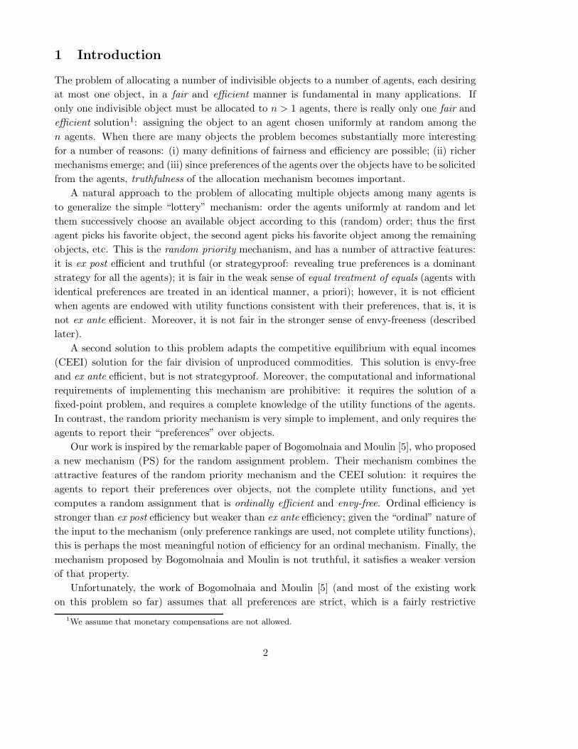
Next, we remove the nodes {4, 5, 6, c} from the network of Figure 2 to get the network

shown in Figure 3. In this network it is clear that for any λ ≤ 1/3, S1 will be the unique min-

cut. As λ is increased further, at λ = 2/3, both S1 and S3 = {s, 1, 2, 3, a, b} have capacity 2 and

are min-cuts. Therefore, λ∗ = 2/3 is the smallest breakpoint for network, and X ∗ = {1, 2, 3}

13

Figure 3: A network

is the bottleneck set. We need to distribute the objects {a, b} among the agents {1, 2, 3} such

that each agent gets 2/3 units of an acceptable object, and we can do so by finding a maximum

flow in this network with λ set to 2/3. But observe that there are multiple ways of achieving

this. For example we could give 1/3 of a and 1/3 of b to 1, 2/3 of b to 2, 2/3 of a to 3; (or)

we could give 2/3 of a to 1, 2/3 of b to 2, 1/3 of a and 1/3 of b to 3. Of course, each agent’s

welfare remains the same in any such solution, so any random assignment is acceptable. One

such solution is:a b c

1 1/3 1/3 0

2 0 2/3 0

3 2/3 0 0

4 0 0 1/3

5 0 0 1/3

6 0 0 1/3

(4)

At this stage, all the objects have been distributed among the agents and so the algorithm

ends.

Properties. We now state some attractive properties of the random assignment found by the

parametric max-flow algorithm. Recall that an n-vector x Lorenz dominates an n-vector y if

and only if upon rearranging their coordinates in increasing order, we have∑k

i=1 xi ≥∑k

i=1 yi,

for all k = 1, 2, . . . , n. An n-vector x is lexicographically greater than an n-vector y if and

only if upon rearranging their coordinates in increasing order, xi is larger than yi in the first

coordinate in which they differ. Note that if x Lorenz dominates y, then x is lexicographically

greater than y, but the converse is not true.

Theorem 1 1. The parametric max-flow algorithm finds a random assignment whose utility

vector is Lorenz dominant. In particular, the random assignment is ordinally efficient.

2. The random assignment P computed by the parametric max-flow algorithm is envy-free.

3. The parametric max-flow mechanism is group strategyproof.

14

Theorem 1 is proved formally in [7], so we will not repeat the proofs here. A weaker version

of the first statement of Theorem 1 is due to Megiddo [19], proved in the context of a sharing

problem, described next.

5.2 The Sharing Problem

The random assignment problem with dichotomous preferences is closely related to the sharing

problem, first introduced by Brown [8]. Brown’s work was partly motivated by a coal-strike

problem: during a coal-strike, some “non-union” mines could still be producing. In this case,

how should the limited supply of coal be distributed equitably among the power companies

that need it? Since power companies vary in size, it would not be desirable to give each power

company the same amount of coal. Moreover, even if such an equal sharing was desirable, the

distribution system may not allow for a perfect distribution because of capacity constraints.

Brown [8] models the distribution system by a network in which there are multiple sources

(representing the coal-producers), multiple sinks (representing power companies), and multiple

transshipment nodes; each edge in the network has a capacity which is an upper bound on

the amount of coal that can traverse that edge. Also, each sink node has a positive “weight”

reflecting its relative importance, and the utility of any sink node is the amount of coal it

receives divided by its weight. The goal is to distribute the supply of coal so as to maximize

the utility of the sink that is worst-off. This maximin objective is in the spirit of Rawls [20].

Following Brown [8], a number of authors have explored a variety of related models, arising in

diverse applications. Itai and Rodeh [16] study the minimax sharing problem (minimize the

utility of the sink that is best-off) and the optimal sharing problem (simultaneously maximizes

the utility of the worst-off sink and minimizes the utility of the best-off sink). In contrast

to these papers in which only one or two of the sinks enter the objective function explicitly,

Megiddo [18, 19] considers the lexicographic sharing problem, where the objective is to lexico-

graphically maximize the utility vector of all the sinks, where the kth component of the utility

vector is the kth smallest utility. The algorithm described earlier in §5.1 is precisely the one

that finds a lex-optimal flow for this sharing problem. We note that flow sharing problems arise

in other contexts as well such as network transmission [15, 16] and network vulnerability [13];

we refer the reader to the paper of Gallo et al. [11] for more details.

6 Random Assignment: The full preference domain

We now extend the parametric max-flow algorithm to compute an envy-free, ordinally efficient

assignment on the full preference domain. (In view of the impossibility result of §4, the

algorithm cannot even be weakly strategyproof).

Algorithm for the full preference domain and its analysis. The algorithm we propose

is an iterative application of parametric maximum flow algorithm that terminates in (at most)

n phases. The network structure remains the same as in Section 5, with each agent having

15

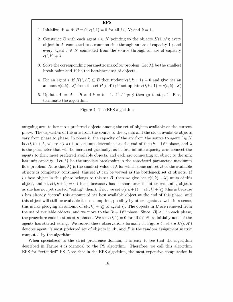
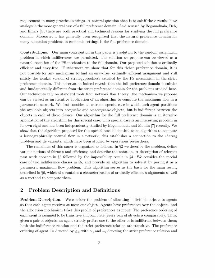
EPS

1. Initialize A′ = A; P ≡ 0; c(i, 1) = 0 for all i ∈ N ; and k = 1.

2. Construct G with each agent i ∈ N pointing to the objects H(i, A′); every

object in A′ connected to a common sink through an arc of capacity 1 ; and

every agent i ∈ N connected from the source through an arc of capacity

c(i, k) + λ .

3. Solve the corresponding parametric max-flow problem. Let λ∗k be the smallest

break point and B be the bottleneck set of objects.

4. For an agent i, if H(i, A′) ⊆ B then update c(i, k + 1) = 0 and give her an

amount c(i, k)+λ∗k from the set H(i, A′) ; if not update c(i, k+1) = c(i, k)+λ∗

k

5. Update A′ = A′ − B and k = k + 1. If A′ 6= φ then go to step 2. Else,

terminate the algorithm.

Figure 4: The EPS algorithm

outgoing arcs to her most preferred objects among the set of objects available at the current

phase. The capacities of the arcs from the source to the agents and the set of available objects

vary from phase to phase. In phase k, the capacity of the arc from the source to agent i ∈ N

is c(i, k) + λ, where c(i, k) is a constant determined at the end of the (k − 1)st phase, and λ

is the parameter that will be increased gradually; as before, infinite capacity arcs connect the

agents to their most preferred available objects, and each arc connecting an object to the sink

has unit capacity. Let λ∗k be the smallest breakpoint in the associated parametric maximum

flow problem. Note that λ∗k is the smallest value of λ for which some subset B of the available

objects is completely consumed; this set B can be viewed as the bottleneck set of objects. If

i’s best object in this phase belongs to this set B, then we give her c(i, k) + λ∗k units of this

object, and set c(i, k + 1) = 0 (this is because i has no share over the other remaining objects

as she has not yet started “eating” them); if not we set c(i, k+1) = c(i, k)+λ∗k (this is because

i has already “eaten” this amount of her best available object at the end of this phase, and

this object will still be available for consumption, possibly by other agents as well; in a sense,

this is like pledging an amount of c(i, k) + λ∗k to agent i). The objects in B are removed from

the set of available objects, and we move to the (k + 1)st phase. Since |B| ≥ 1 in each phase,

the procedure ends in at most n phases. We set c(i, 1) = 0 for all i ∈ N , as initially none of the

agents has started eating. We record these observations formally in Figure 4, where H(i, A ′)

denotes agent i’s most preferred set of objects in A′, and P is the random assignment matrix

computed by the algorithm.

When specialized to the strict preference domain, it is easy to see that the algorithm

described in Figure 4 is identical to the PS algorithm. Therefore, we call this algorithm

EPS for “extended” PS. Note that in the EPS algorithm, the most expensive computation is

16

solving the parametric maximum flow problem. As noted before, the complexity of parametric

maximum flow algorithm is O(nm log(n2/m)), where m is the number of arcs in the network.

Therefore, the overall complexity of the algorithm EPS is O(∑r

k=1 n2mk log(n2/mk)), where

mk is the number of arcs in the kth phase and r is the total number of phases.

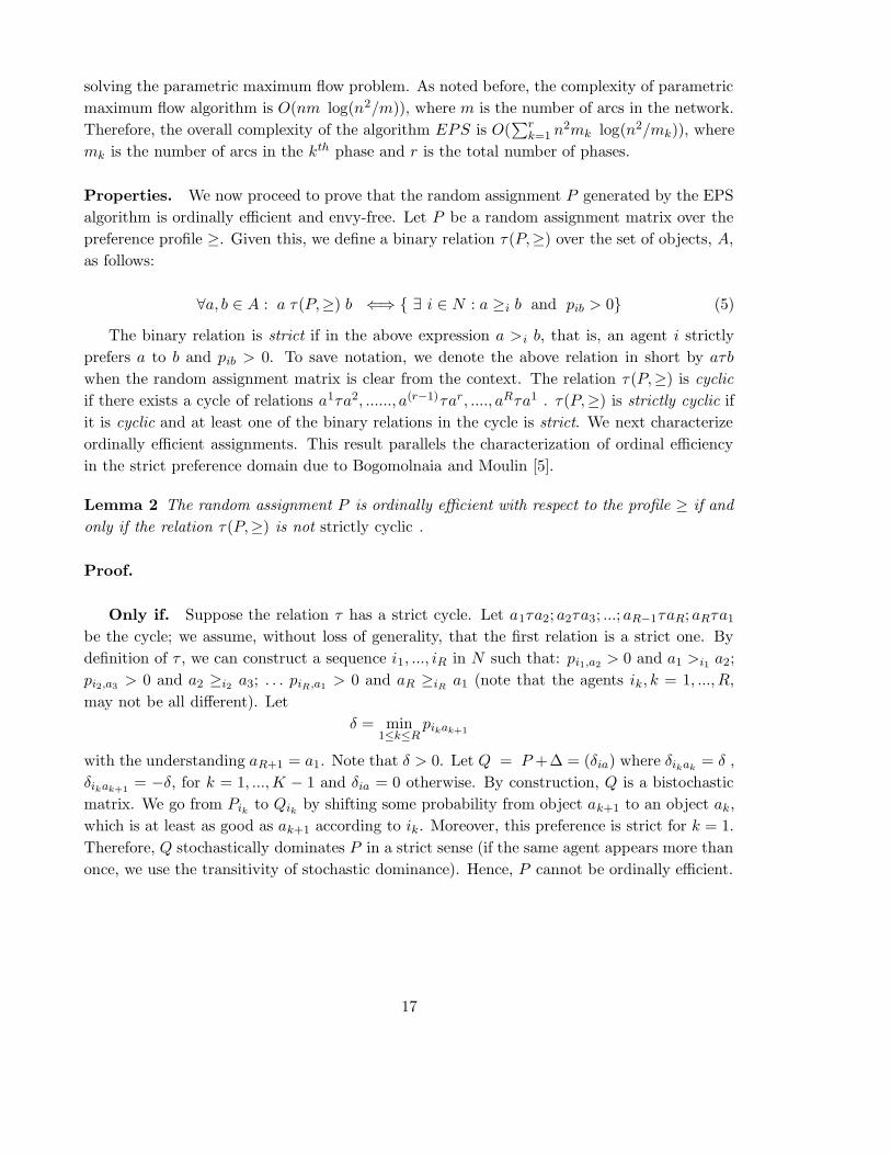
Properties. We now proceed to prove that the random assignment P generated by the EPS

algorithm is ordinally efficient and envy-free. Let P be a random assignment matrix over the

preference profile ≥. Given this, we define a binary relation τ(P,≥) over the set of objects, A,

as follows:

∀a, b ∈ A : a τ(P,≥) b ⇐⇒ { ∃ i ∈ N : a ≥i b and pib > 0} (5)

The binary relation is strict if in the above expression a >i b, that is, an agent i strictly

prefers a to b and pib > 0. To save notation, we denote the above relation in short by aτb

when the random assignment matrix is clear from the context. The relation τ(P,≥) is cyclic

if there exists a cycle of relations a1τa2, ......, a(r−1)τar, ...., aRτa1 . τ(P,≥) is strictly cyclic if

it is cyclic and at least one of the binary relations in the cycle is strict. We next characterize

ordinally efficient assignments. This result parallels the characterization of ordinal efficiency

in the strict preference domain due to Bogomolnaia and Moulin [5].

Lemma 2 The random assignment P is ordinally efficient with respect to the profile ≥ if and

only if the relation τ(P,≥) is not strictly cyclic .

Proof.

Only if. Suppose the relation τ has a strict cycle. Let a1τa2; a2τa3; ...; aR−1τaR; aRτa1

be the cycle; we assume, without loss of generality, that the first relation is a strict one. By

definition of τ , we can construct a sequence i1, ..., iR in N such that: pi1,a2> 0 and a1 >i1 a2;

pi2,a3> 0 and a2 ≥i2 a3; . . . piR,a1

> 0 and aR ≥iR a1 (note that the agents ik, k = 1, ..., R,

may not be all different). Let

δ = min1≤k≤R

pikak+1

with the understanding aR+1 = a1. Note that δ > 0. Let Q = P +∆ = (δia) where δikak= δ ,

δikak+1= −δ, for k = 1, ...,K − 1 and δia = 0 otherwise. By construction, Q is a bistochastic

matrix. We go from Pik to Qik by shifting some probability from object ak+1 to an object ak,

which is at least as good as ak+1 according to ik. Moreover, this preference is strict for k = 1.

Therefore, Q stochastically dominates P in a strict sense (if the same agent appears more than

once, we use the transitivity of stochastic dominance). Hence, P cannot be ordinally efficient.

17

If. Suppose P is not ordinally efficient. Let Q be a matrix than stochastically dominates

P , and let i1 be an agent for whom Qi1 6= Pi1 . By definition of stochastic dominance, there

exist two objects a1, a2 such that

a1 >i1 a2; qi1,a1> pi1,a1

and qi1,a2< pi1,a2

(6)

In other words, a1τ(P,≥)a2 in a strict sense. Next by the feasibility of Q, there exists an agent

i2 such that qi2,a2> pi2a2

. Repeating the argument, we find an a3 such that a2 ≥i2 a3 and

pi2,a3> qi2,a3

; and hence a2τa3. Due to finiteness of A and N , we will eventually find a cycle

of the relation τ . If this cycle contains a1 (or) if this cycle is strict, then we are done.

Now suppose that the cycle is not strict. Let the cycle be made up of the objects

(b1, b2, . . . , bn) and the corresponding agents be (i1, i2, . . . , in). Note that we will have qi1,b2 <

1, . . . , qin−1,bn< 1, qin,b1 < 1 and qi1,b1 > 0, . . . , qin,bn

> 0. Also note that we will have

b1 =i1 b2, . . . , bn =in b1 (as the cycle is not strict). Now we make the following transformation

: q′i1,b1= qi1,b1 − δ, q′i1,b2

= qi1,b2 + δ, . . . , q′in,bn= qin,bn

− δ, q′in ,b1= qin,b1 + δ, and for all other

i ∈ N, j ∈ A; q′i, j = qi,j, where

δ = max{k : qij ,aj− k ≥ pij ,aj

, qij ,aj+1+ k ≤ pij ,aj+1

∀i = 1, · · · , n} (7)

Note that the new matrix Q′ still stochastically dominates P in a strict sense. Now if we

repeat the exercise of finding a cycle for this matrix Q′, we will never find the cycle which we

found in Q ( because for one particular (agent,object) pair, say (i,c), involved in the cycle we

have made q′(i, c) = p(i, c) and hence this pair will never enter the cycle in the future). Since

the number of nonstrict cycles is finite, we will eventually find a strict cycle of the relation τ .

We are now ready to prove that the EPS algorithm finds an ordinally efficient assignment.

Theorem 3 The algorithm proposed is ordinally efficient.

Proof. Suppose not. Then, by Lemma 2, we can find a cycle in the relation τ over the

assignment matrix Q: a1τa2, . . . , arτar+1, . . . , aRτa1. Without loss of generality, assume that

the last binary relation is strict. Let ir be an agent such that ar ≥ir ar+1 and pir,ar+1 > 0

(r ∈ 1, . . . , R, with the convention aR+1 = a1). Let sr be the phase of the EPS algorithm

during which ar was in the bottleneck set. Since ar is at least as good as ar+1 for the agent ir,

and ir gets a positive amount of ar+1 , ar+1 could not have been in the bottleneck set before

ar. Therefore, sr ≤ sr+1. Moreover, if ar is strictly preferred over ar+1 , then sr < sr+1.

Note that sR+1 = s1.Therefore, s1 ≤ s2 ≤ . . . ≤ sR < s1. But, this is a contradiction because

s0 = sR+1. Therefore, the algorithm is ordinally efficient.

Next, we prove the that assignment P found by the EPS algorithm is envy-free.

Theorem 4 The matrix P given by the EPS algorithm is envy-free.

18

Proof. Let the preference profile be ≥. Consider any two agents i, j ∈ N and an object

a ∈ A. Define the set M(i, a) = {b : b ≥i a}. Let k be the first phase of the algorithm by the

end of which all the objects in M(i, a) are used up. Note that in the first k phases, i will be

allocated objects only from the set M(i, a). Therefore, the number of units allocated to i from

the objects in M(i, a) is∑

l∈M(i,a) pi,l = λ∗1 + . . . +λ∗

k ≥∑

l∈M(i,a) pj,l (since j could have used

some other objects outside the set M(i, a)). Therefore, i cannot envy j and hence EPS always

finds an envy-free random assignment.

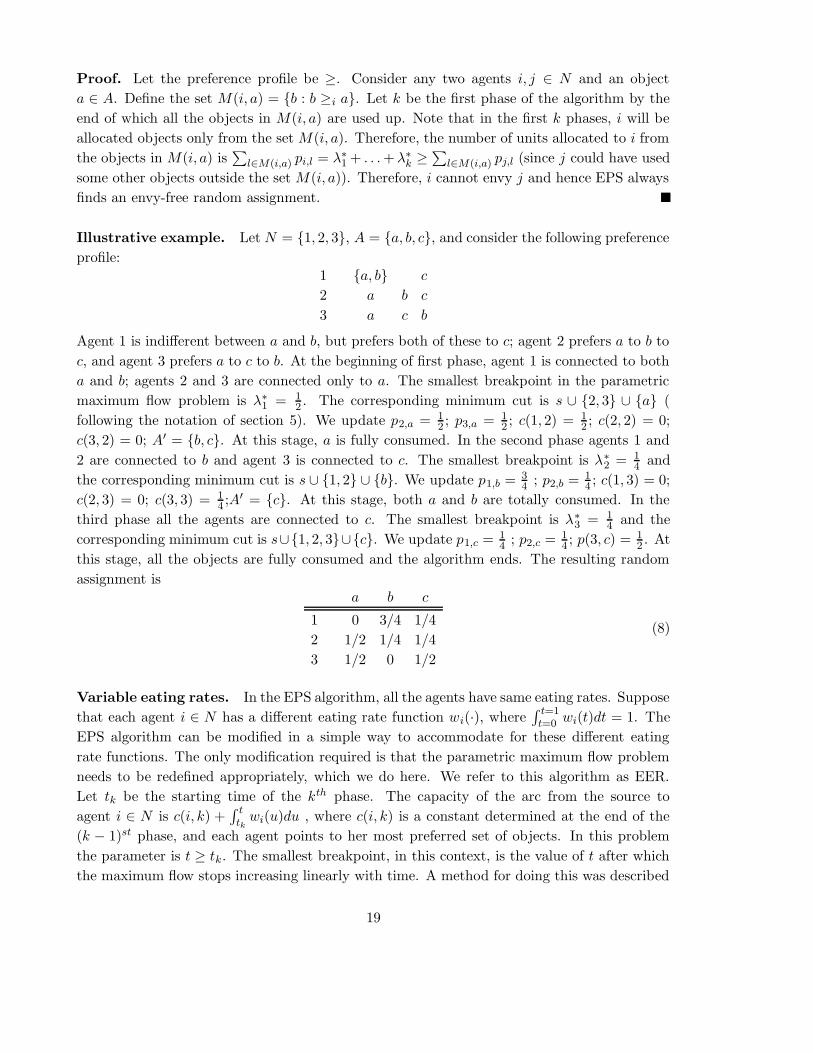
Illustrative example. Let N = {1, 2, 3}, A = {a, b, c}, and consider the following preference

profile:1 {a, b} c

2 a b c

3 a c b

Agent 1 is indifferent between a and b, but prefers both of these to c; agent 2 prefers a to b to

c, and agent 3 prefers a to c to b. At the beginning of first phase, agent 1 is connected to both

a and b; agents 2 and 3 are connected only to a. The smallest breakpoint in the parametric

maximum flow problem is λ∗1 = 1

2 . The corresponding minimum cut is s ∪ {2, 3} ∪ {a} (

following the notation of section 5). We update p2,a = 12 ; p3,a = 1

2 ; c(1, 2) = 12 ; c(2, 2) = 0;

c(3, 2) = 0; A′ = {b, c}. At this stage, a is fully consumed. In the second phase agents 1 and

2 are connected to b and agent 3 is connected to c. The smallest breakpoint is λ∗2 = 1

4 and

the corresponding minimum cut is s ∪ {1, 2} ∪ {b}. We update p1,b = 34 ; p2,b = 1

4 ; c(1, 3) = 0;

c(2, 3) = 0; c(3, 3) = 14 ;A′ = {c}. At this stage, both a and b are totally consumed. In the

third phase all the agents are connected to c. The smallest breakpoint is λ∗3 = 1

4 and the

corresponding minimum cut is s∪{1, 2, 3}∪{c}. We update p1,c = 14 ; p2,c = 1

4 ; p(3, c) = 12 . At

this stage, all the objects are fully consumed and the algorithm ends. The resulting random

assignment isa b c

1 0 3/4 1/4

2 1/2 1/4 1/4

3 1/2 0 1/2

(8)

Variable eating rates. In the EPS algorithm, all the agents have same eating rates. Suppose

that each agent i ∈ N has a different eating rate function wi(·), where∫ t=1t=0 wi(t)dt = 1. The

EPS algorithm can be modified in a simple way to accommodate for these different eating

rate functions. The only modification required is that the parametric maximum flow problem

needs to be redefined appropriately, which we do here. We refer to this algorithm as EER.

Let tk be the starting time of the kth phase. The capacity of the arc from the source to

agent i ∈ N is c(i, k) +∫ t

tkwi(u)du , where c(i, k) is a constant determined at the end of the

(k − 1)st phase, and each agent points to her most preferred set of objects. In this problem

the parameter is t ≥ tk. The smallest breakpoint, in this context, is the value of t after which

the maximum flow stops increasing linearly with time. A method for doing this was described

19

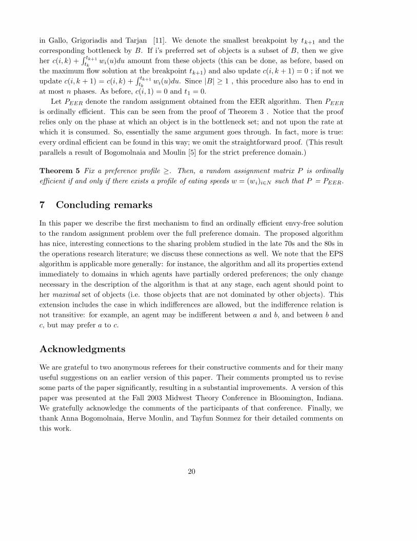
in Gallo, Grigoriadis and Tarjan [11]. We denote the smallest breakpoint by tk+1 and the

corresponding bottleneck by B. If i’s preferred set of objects is a subset of B, then we give

her c(i, k) +∫ tk+1

tkwi(u)du amount from these objects (this can be done, as before, based on

the maximum flow solution at the breakpoint tk+1) and also update c(i, k + 1) = 0 ; if not we

update c(i, k + 1) = c(i, k) +∫ tk+1

tkwi(u)du. Since |B| ≥ 1 , this procedure also has to end in

at most n phases. As before, c(i, 1) = 0 and t1 = 0.

Let PEER denote the random assignment obtained from the EER algorithm. Then PEER

is ordinally efficient. This can be seen from the proof of Theorem 3 . Notice that the proof

relies only on the phase at which an object is in the bottleneck set; and not upon the rate at

which it is consumed. So, essentially the same argument goes through. In fact, more is true:

every ordinal efficient can be found in this way; we omit the straightforward proof. (This result

parallels a result of Bogomolnaia and Moulin [5] for the strict preference domain.)

Theorem 5 Fix a preference profile ≥. Then, a random assignment matrix P is ordinally

efficient if and only if there exists a profile of eating speeds w = (wi)i∈N such that P = PEER.

7 Concluding remarks

In this paper we describe the first mechanism to find an ordinally efficient envy-free solution

to the random assignment problem over the full preference domain. The proposed algorithm

has nice, interesting connections to the sharing problem studied in the late 70s and the 80s in

the operations research literature; we discuss these connections as well. We note that the EPS

algorithm is applicable more generally: for instance, the algorithm and all its properties extend

immediately to domains in which agents have partially ordered preferences; the only change

necessary in the description of the algorithm is that at any stage, each agent should point to

her maximal set of objects (i.e. those objects that are not dominated by other objects). This

extension includes the case in which indifferences are allowed, but the indifference relation is

not transitive: for example, an agent may be indifferent between a and b, and between b and

c, but may prefer a to c.

Acknowledgments

We are grateful to two anonymous referees for their constructive comments and for their many

useful suggestions on an earlier version of this paper. Their comments prompted us to revise

some parts of the paper significantly, resulting in a substantial improvements. A version of this

paper was presented at the Fall 2003 Midwest Theory Conference in Bloomington, Indiana.

We gratefully acknowledge the comments of the participants of that conference. Finally, we

thank Anna Bogomolnaia, Herve Moulin, and Tayfun Sonmez for their detailed comments on

this work.

20

References

[1] A.Abdulkadiroglu and T.Sonmez (1998), “Random serial dictatorship and the core from

random endowments in house allocation problems”, Econometrica, 66, 689–701.

[2] A.Abdulkadiroglu and T.Sonmez (2003), “Ordinal efficiency and dominated sets of assign-

ments,” Journal of Economic Theory, 112, 157-172.

[3] Ahuja, Magnanti and Orlin ,“ Network Flows: Theory, Algorithms, and Applications”,

Prentice Hall, 1993.

[4] A. Bogomolnaia, R. Deb and L. Ehlers , “Strategy-proof assignment on the full preference

domain”, Journal of Economic Theory, forthcoming.

[5] A.Bogomolnaia and H. Moulin (2001), “A new solution to the Random Assignment prob-

lem”, Journal of Economic Theory, 100, 295–328.

[6] A. Bogomolnaia and H. Moulin (2002), “A Simple Random Assignment Problem with a

Unique Solution”, Economic Theory, 19, 623–636.

[7] A. Bogomolnaia and H. Moulin (2004), “Random Matching under Dichotomous prefer-

ences”, Econometrica, 72, 257–279.

[8] J.R.Brown (1979),“The sharing problem”, Oper. Res. , 27, 324–340.

[9] H. Cres and H. Moulin (2001), “Scheduling with Opting Out: Improving upon Random

Priority”, Operations Research, 49(4):565–576.

[10] D. Gale (1987), “College course assignments and optimal lotteries”, mimeo, University of

California, Berkeley, 1987.

[11] Giorgio Gallo, Michael D Grigoriadis and Robert E Tarjan (1989),“A Fast Parametric

Maximum Flow Algorithm and Applications”, SIAM J. Comput. , 18, 30–55.

[12] A.V.Goldberg and R.E.Tarjan , “A new approach to the maximum flow problem”, Proc.

18h Annual ACM Symposium on Theory of Computing, 1986, 136–146; J. Assoc. Comput.

Mach., 35 (1988).

[13] D.Gusfield (1987),“Computing the strength of a network in O(|V |3|E|) time”, Tech. report

CSE-87-2, Department of Electrical and Computer Engineering, University of California,

Davis, CA.

[14] A.Hylland and R.Zeckhauser (1979), “The efficient allocation of individuals to positions”,

J. Polit. Econ. , 91, 293–313.

[15] T.Ichimori, H.Ishii and T.Nishida (1982),“Optimal sharing”, Math. Programming, 23,

341–348.

21

[16] A.Itai and M.Rodeh (1985),“Scheduling transmissions in a network”, J. Algorithms, 6,

409–429.

[17] A. McLennan (2002), “Ordinal efficiency and the polyhedral separating hyperplane theo-

rem,” Journal of Economic Theory, 105, 435–449.

[18] N. Megiddo (1974),“Optimal flows in networks with multiple sources and sinks”, Math.

Programming, 7, 97–107.

[19] N. Megiddo (1979),“A good algorithm for lexicographically optimal flows in multi-terminal

networks”, Bull. Amer. Math. Soc., 83, 407–409.

[20] J. Rawls (1971), A Theory of Justice, Harvard University Press, Cambridge, MA.

[21] A. E. Roth (1982), “Incentive compatibility in a market with indivisibilities,” Economics

Letters, 9, 127–132.

[22] A. E. Roth and A. Postlewaite (1977), “Weak versus strong domination in a market with

indivisible goods,” Journal of Mathematical Economics, 4, 131–137.

[23] L. Shapley and H. Scarf (1974), “On cores and indivisibility,” Journal of Mathematical

Economics, 1, 23–28.

[24] L. Svensson (1994), “Queue allocation of indivisible goods”, Soc. Choice Welfare, 11,

323–330.

[25] L. Svensson (1999), “Strategy-proof allocation of indivisible goods”, Soc. Choice Welfare,

16, 557–567.

[26] L. Zhou (1990), “On a conjecture by Gale about one-sided matching problems,” Journal

of Economic Theory, 52, 123–135.

22