A SOFTWARE PACKAGE FOR THE EVALUATION OF …powers/ame.60636/transport.pdf · GAS-PHASE, MULTICOMPONENT TRANSPORT PROPERTIES ... INTRODUCTION ... Dkj Binary diffusion coefficient

TRA-036-1 CHEMKIN Collection Release 3.6 September 2000

TRANSPORT

A SOFTWARE PACKAGE FOR THE EVALUATION OF GAS-PHASE, MULTICOMPONENT

TRANSPORT PROPERTIES

Reaction Design

2

Licensing:Licensing:Licensing:Licensing: For licensing information, please contact Reaction Design. (858) 550-1920 (USA) or [email protected]

Technical Support:Technical Support:Technical Support:Technical Support: Reaction Design provides an allotment of technical support to its Licensees free of charge. To request technical support, please include your license number along with input or output files, and any error messages pertaining to your question or problem. Requests may be directed in the following manner: E-Mail: [email protected], Fax: (858) 550-1925, Phone: (858) 550-1920. Technical support may also be purchased. Please contact Reaction Design for the technical support hourly rates at [email protected] or (858) 550-1920 (USA).

Copyright:Copyright:Copyright:Copyright: Copyright© 2000 Reaction Design. All rights reserved. No part of this book may be reproduced in any form or by any means without express written permission from Reaction Design.

Trademark:Trademark:Trademark:Trademark: AURORA, CHEMKIN, The CHEMKIN Collection, CONP, CRESLAF, EQUIL, Equilib, OPPDIF, PLUG, PREMIX, Reaction Design, SENKIN, SHOCK, SPIN, SURFACE CHEMKIN, SURFTHERM, TRANSPORT, TWOPNT are all trademarks of Reaction Design or Sandia National Laboratories.

Limitation of Warranty:Limitation of Warranty:Limitation of Warranty:Limitation of Warranty: The software is provided “as is” by Reaction Design, without warranty of any kind including without limitation, any warranty against infringement of third party property rights, fitness or merchantability, or fitness for a particular purpose, even if Reaction Design has been informed of such purpose. Furthermore, Reaction Design does not warrant, guarantee, or make any representations regarding the use or the results of the use, of the software or documentation in terms of correctness, accuracy, reliability or otherwise. No agent of Reaction Design is authorized to alter or exceed the warranty obligations of Reaction Design as set forth herein. Any liability of Reaction Design, its officers, agents or employees with respect to the software or the performance thereof under any warranty, contract, negligence, strict liability, vicarious liability or other theory will be limited exclusively to product replacement or, if replacement is inadequate as a remedy or in Reaction Design’s opinion impractical, to a credit of amounts paid to Reaction Design for the license of the software.

Literature Citation for Literature Citation for Literature Citation for Literature Citation for TTTTRANSPORTRANSPORTRANSPORTRANSPORT:::: The TRANSPORT program and subroutine library are part of the CHEMKIN Collection. R. J. Kee, F. M. Rupley, J. A. Miller, M. E. Coltrin, J. F. Grcar, E. Meeks, H. K. Moffat, A. E. Lutz, G. Dixon-Lewis, M. D. Smooke, J. Warnatz, G. H. Evans, R. S. Larson, R. E. Mitchell, L. R. Petzold, W. C. Reynolds, M. Caracotsios, W. E. Stewart, P. Glarborg, C. Wang, and Ola Adigun, CHEMKIN Collection, Release 3.6, Reaction Design, Inc., San Diego, CA (2000).

Acknowledgements:Acknowledgements:Acknowledgements:Acknowledgements: This document is based on the Sandia National Laboratories Report SAND86-8246B, authored by R. J. Kee, G. Dixon-Lewis, J. Warnatz, M. E. Coltrin, J. A. Miller, H. K. Moffat.1

Reaction Design cautions that some of the material in this manual may be out of date. Updates will be available periodically on Reaction Design's web site. In addition, on-line help is available on the program CD. Sample problem files can also be found on the CD and on our web site at www.ReactionDesign.com.

3

TRA-036-1

TRANSPORTTRANSPORTTRANSPORTTRANSPORT: A SOFTWARE PACKAGE FOR THE EVALUATION: A SOFTWARE PACKAGE FOR THE EVALUATION: A SOFTWARE PACKAGE FOR THE EVALUATION: A SOFTWARE PACKAGE FOR THE EVALUATION OF GASOF GASOF GASOF GAS----PHASE, MULTICOMPONENTPHASE, MULTICOMPONENTPHASE, MULTICOMPONENTPHASE, MULTICOMPONENT

TRANTRANTRANTRANSPORT PROPERTIESSPORT PROPERTIESSPORT PROPERTIESSPORT PROPERTIES

ABSTRACTABSTRACTABSTRACTABSTRACT TRANSPORT is a software package that is used for the evaluation of gas-phase multicomponent viscosities, thermal conductivities, diffusion coefficients, and thermal diffusion coefficients for CHEMKIN Applications. The TRANSPORT Property package consists of two parts. The first is a preprocessor that computes polynomial fits to the temperature-dependent parts of the pure species viscosities and binary diffusion coefficients. The coefficients of these fits are passed to a library of subroutines via a Linking File. Then, any subroutine from the TRANSPORT Subroutine Library may be called from a CHEMKIN Application to return either pure species properties or multicomponent gas mixture properties. The TRANSPORT Property package interfaces with the CHEMKIN Gas-phase Subroutine Library.

5

CONTENTSCONTENTSCONTENTSCONTENTS Page FIGURES...................................................................................................................................................................... 6 NOMENCLATURE.................................................................................................................................................... 7 1. INTRODUCTION ............................................................................................................................................. 10 2. THE TRANSPORT EQUATIONS ................................................................................................................... 12

2.1 Pure Species Viscosity and Binary Diffusion Coefficients ................................................................ 12 2.2 Pure Species Thermal Conductivities .................................................................................................. 14 2.3 The Pure-Species Fitting Procedure..................................................................................................... 17 2.4 The Mass, Momentum, and Energy Fluxes ........................................................................................ 18 2.5 The Mixture-Averaged Properties ....................................................................................................... 21 2.6 Thermal Diffusion Ratios ...................................................................................................................... 21 2.7 The Multicomponent Properties........................................................................................................... 23 2.8 Species Conservation ............................................................................................................................. 27

3. THE MECHANICS OF USING THE PACKAGE ......................................................................................... 29 3.1 General Flow of Information ................................................................................................................ 29 3.2 Accessing the Transport Property Subroutine Library from an Application................................. 29 3.3 Use of Command-Line Arguments...................................................................................................... 30

4. QUICK REFERENCE TO THE TRANSPORT SUBROUTINE LIBRARY.................................................. 31 4.1 Mnemonics .............................................................................................................................................. 31 4.2 Initialization and Parameters................................................................................................................ 32 4.3 Viscosity................................................................................................................................................... 32 4.4 Conductivity ........................................................................................................................................... 33 4.5 Diffusion Coefficients ............................................................................................................................ 33 4.6 Thermal Diffusion .................................................................................................................................. 33

5. ALPHABETICAL LISTING OF THE TRANSPORT SUBROUTINE LIBRARY WITH DETAILED DESCRIPTIONS OF THE CALL LISTS.......................................................................................................... 35

6. TRANSPORT DATABASE .............................................................................................................................. 44 7. REFERENCES.................................................................................................................................................... 51

6

FIGURESFIGURESFIGURESFIGURES Page

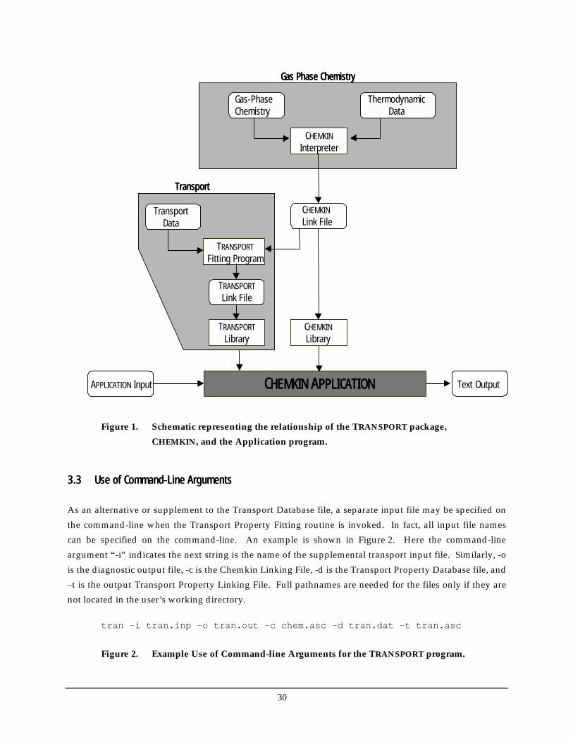
Figure 1. Schematic representing the relationship of the TRANSPORT package, CHEMKIN, and the Application program............................................................................................................................ 30

Figure 2. Example Use of Command-line Arguments for the TRANSPORT program.................................. 30

7

NOMENCLATURENOMENCLATURENOMENCLATURENOMENCLATURE CGS Units

ck Specific heat at constant volume of the kth species in mass units ergs/(g K)

ck, int. Internal contribution to the mass specific heat of the kth species ergs/(g K)

ck, rot. Rotational contribution to the mass specific heat of the kth species ergs/(g K)

Cv, rot. Rotational contribution to the molar specific heat of the species ergs/(mole K)

Ck, trans. Translational contribution to the molar specific heat of the species ergs/(mole K)

Ck, vib. Vibrational contribution to the molar specific heat of the species ergs/(mole K) kjD Binary diffusion coefficient of species k in species j cm2/sec

Dkm Mixture-averaged diffusion coefficient of the kth species cm2/sec

Dk,j Multicomponent diffusion coefficient of the species k in species j cm2/sec T

kD Thermal diffusion coefficient of the kth species cm2/sec

hk Enthalpy of the kth species ergs/g

jk Diffusive mass flux of the kth species ergs/g

k Species index ---

kB Boltzmann Constant ergs/K

K Total number of species ---

mk Molecular mass of the kth species g

mjk Reduced molecular mass for the collision g

n Species index for a non-polar species ---

p Species index for a polar species ---

p Pressure dynes/cm2

q Heat flux ergs/(cm2 sec)

R Universal gas constant ergs/(mole K)

T Temperature K *kT Reduced temperature of the kth species --- *jkT Reduced temperature for the collision ---

υ Velocity vector cm/sec

Vk Diffusion velocity of the kth species cm/sec

Vk Ordinary diffusion velocity of the kth species cm/sec

Wk Molecular weight of kth species g/mole

Wk Thermal diffusion velocity of kth species cm/sec

W Mean molecular weight of a mixture g/mole

Xk Mole fraction of the kth species ---

Yk Mass fraction of the kth species ---

8

GREEK

CGS Units

kα Polarizability of the kth species Å3

*kα Reduced polarizability of the kth species ---

δ Unit tensor in Eq. 37 ---

δ Small number (e.g. 1.E-12) --- *kδ Reduced dipole moment of the kth species --- *jkδ Effective reduced dipole moment for the collison ---

ε Small number (e.g. 1.E-12) ---

kε Lennard-Jones potential well depth for the kth species ergs

jkε Effective Lennard-Jones potential well depth for the collision ergs

η Mixture viscosity g/(cm sec)

kη Pure species viscosity of the kth species g/(cm sec)

κ Bulk coefficient of viscosity g/(cm sec)

λ Thermal conductivity of the gas mixture ergs/(cm K sec)

kλ Thermal conductivity of the kth species ergs/(cm K sec)

0λ Multicomponent thermal conductivity of the species ergs/(cm K sec)

kµ Dipole moment of the kth species Debye *kµ Reduced dipole moment of the kth species ---

jkµ Effective dipole moment for the collision Debye

ijξ Relaxation collision number ---

ρ Mass density g/cm3

kσ Lennard-Jones diameter Å

jkσ Effective Lennard-Jones diameter for the collision Å

τ Momentum flux g/(cm sec2)

Θk Thermal diffusion ratio for mixture-averaged formula ---

Ω Collision integral ---

9

10

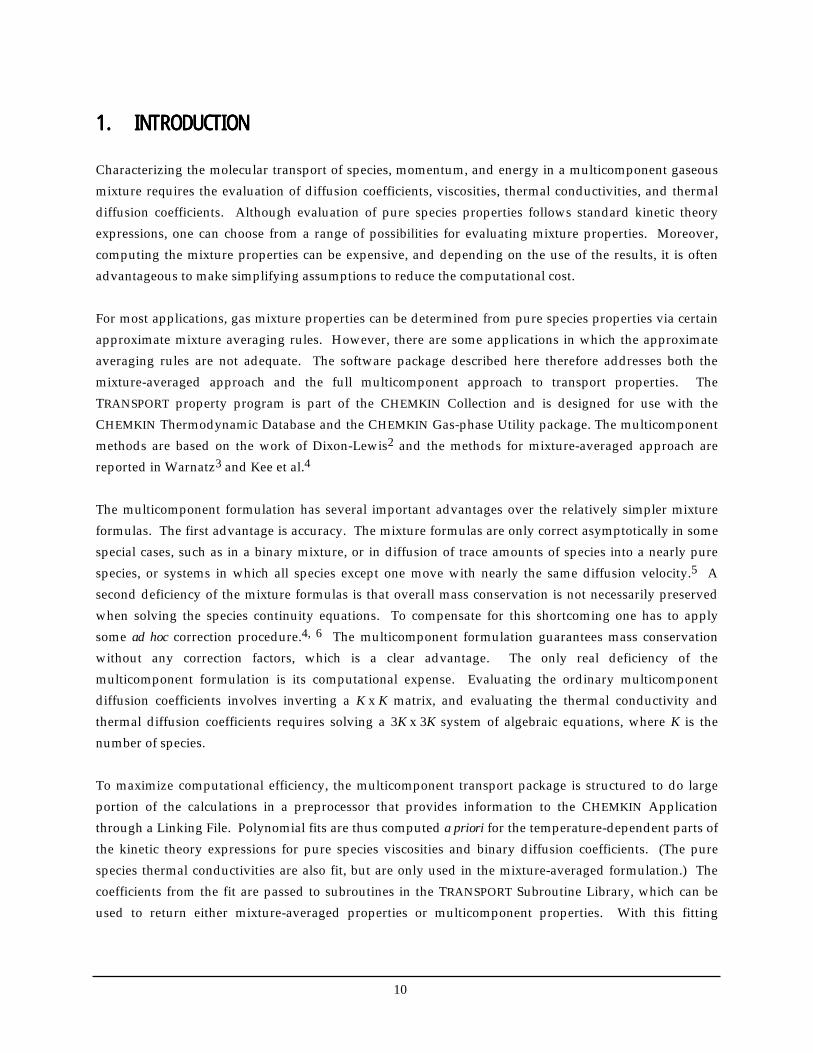
1.1.1.1. INTRODUCTIONINTRODUCTIONINTRODUCTIONINTRODUCTION Characterizing the molecular transport of species, momentum, and energy in a multicomponent gaseous mixture requires the evaluation of diffusion coefficients, viscosities, thermal conductivities, and thermal diffusion coefficients. Although evaluation of pure species properties follows standard kinetic theory expressions, one can choose from a range of possibilities for evaluating mixture properties. Moreover, computing the mixture properties can be expensive, and depending on the use of the results, it is often advantageous to make simplifying assumptions to reduce the computational cost. For most applications, gas mixture properties can be determined from pure species properties via certain approximate mixture averaging rules. However, there are some applications in which the approximate averaging rules are not adequate. The software package described here therefore addresses both the mixture-averaged approach and the full multicomponent approach to transport properties. The TRANSPORT property program is part of the CHEMKIN Collection and is designed for use with the CHEMKIN Thermodynamic Database and the CHEMKIN Gas-phase Utility package. The multicomponent methods are based on the work of Dixon-Lewis2 and the methods for mixture-averaged approach are reported in Warnatz3 and Kee et al.4 The multicomponent formulation has several important advantages over the relatively simpler mixture formulas. The first advantage is accuracy. The mixture formulas are only correct asymptotically in some special cases, such as in a binary mixture, or in diffusion of trace amounts of species into a nearly pure species, or systems in which all species except one move with nearly the same diffusion velocity.5 A second deficiency of the mixture formulas is that overall mass conservation is not necessarily preserved when solving the species continuity equations. To compensate for this shortcoming one has to apply some ad hoc correction procedure.4, 6 The multicomponent formulation guarantees mass conservation without any correction factors, which is a clear advantage. The only real deficiency of the multicomponent formulation is its computational expense. Evaluating the ordinary multicomponent diffusion coefficients involves inverting a K x K matrix, and evaluating the thermal conductivity and thermal diffusion coefficients requires solving a 3K x 3K system of algebraic equations, where K is the number of species. To maximize computational efficiency, the multicomponent transport package is structured to do large portion of the calculations in a preprocessor that provides information to the CHEMKIN Application through a Linking File. Polynomial fits are thus computed a priori for the temperature-dependent parts of the kinetic theory expressions for pure species viscosities and binary diffusion coefficients. (The pure species thermal conductivities are also fit, but are only used in the mixture-averaged formulation.) The coefficients from the fit are passed to subroutines in the TRANSPORT Subroutine Library, which can be used to return either mixture-averaged properties or multicomponent properties. With this fitting

11

procedure, expensive operations, such as evaluation of collision integrals, are only done once and not every time a property is needed. Chapter 2 of this manual first reviews the kinetic theory expressions for the pure species viscosities and the binary diffusion coefficients. Section 2.4 describes how momentum, energy, and species mass fluxes are computed from the velocity, temperature and species gradients and either mixture-averaged or multicomponent transport properties. Based on these concepts, Sections 2.5 - 2.7 describe the procedures to determine multicomponent transport properties from the pure species expressions. Chapter 3 outlines how to use the TRANSPORT software package and how it relates to the CHEMKIN Gas-phase Utilities. Chapters 4 and 5 include details on each of the multicomponent subroutines that can be called by a CHEMKIN Application program. Finally, Chapter 6 lists the database that is currently provided with the TRANSPORT software.

12

2.2.2.2. THE TRANSPORT EQUATIONSTHE TRANSPORT EQUATIONSTHE TRANSPORT EQUATIONSTHE TRANSPORT EQUATIONS

2.12.12.12.1 Pure Species Viscosity and Binary Diffusion CoefficientsPure Species Viscosity and Binary Diffusion CoefficientsPure Species Viscosity and Binary Diffusion CoefficientsPure Species Viscosity and Binary Diffusion Coefficients

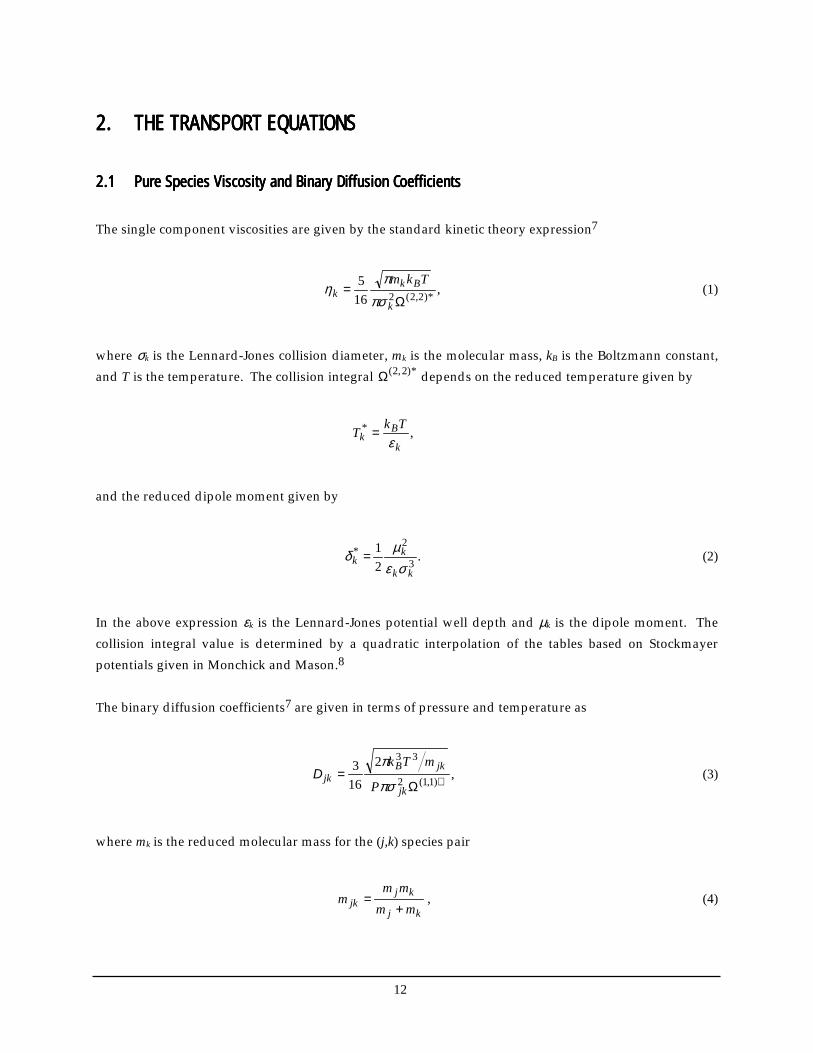
The single component viscosities are given by the standard kinetic theory expression7

,165

*)2,2(2Ω=

k

Bkk

Tkm

πσ

πη (1)

where σk is the Lennard-Jones collision diameter, mk is the molecular mass, kB is the Boltzmann constant, and T is the temperature. The collision integral Ω(2,2)* depends on the reduced temperature given by

,*

k

Bk

TkTε

=

and the reduced dipole moment given by

.21

3

2*

kk

kk

σεµδ = (2)

In the above expression εk is the Lennard-Jones potential well depth and µk is the dipole moment. The collision integral value is determined by a quadratic interpolation of the tables based on Stockmayer potentials given in Monchick and Mason.8 The binary diffusion coefficients7 are given in terms of pressure and temperature as

,2

163

)1,1(2

33

∗Ω=

jk

jkBjk

P

mTk

πσ

πD (3)

where mk is the reduced molecular mass for the (j,k) species pair

kj

kjjk mm

mmm

+= , (4)

13

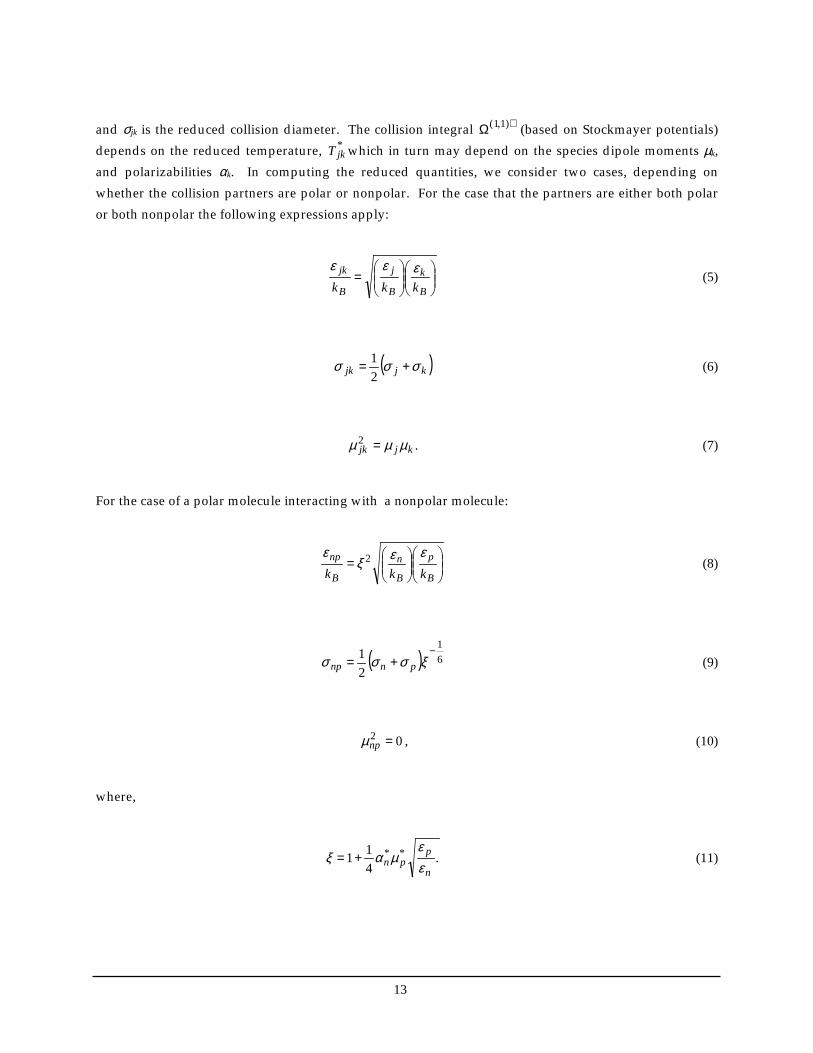
and σjk is the reduced collision diameter. The collision integral Ω(1,1)∗ (based on Stockmayer potentials) depends on the reduced temperature, T jk

* which in turn may depend on the species dipole moments µk, and polarizabilities αk. In computing the reduced quantities, we consider two cases, depending on whether the collision partners are polar or nonpolar. For the case that the partners are either both polar or both nonpolar the following expressions apply:

=

B

k

B

j

B

jk

kkkεεε

(5)

( )kjjk σσσ +=21 (6)

.2kjjk µµµ = (7)

For the case of a polar molecule interacting with a nonpolar molecule:

=

B

p

B

n

B

np

kkkεεξ

ε 2 (8)

( ) 61

21 −

+= ξσσσ pnnp (9)

02 =npµ , (10)

where,

.411 **

n

ppn ε

εµαξ += (11)

14

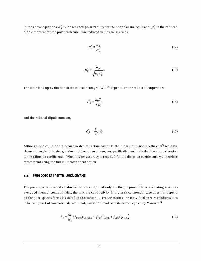
In the above equations *nα is the reduced polarizability for the nonpolar molecule and *

pµ is the reduced dipole moment for the polar molecule. The reduced values are given by

3*

n

nn

σαα = (12)

.3

*

pp

pp

σε

µµ = (13)

The table look-up evaluation of the collision integral ∗Ω )1,1( depends on the reduced temperature

,*

jk

Bjk

TkTε

= (14)

and the reduced dipole moment,

.21 2* ∗= jkjk µδ (15)

Although one could add a second-order correction factor to the binary diffusion coefficients9 we have chosen to neglect this since, in the multicomponent case, we specifically need only the first approximation to the diffusion coefficients. When higher accuracy is required for the diffusion coefficients, we therefore recommend using the full multicomponent option.

2.22.22.22.2 Pure Species Thermal ConductivitiesPure Species Thermal ConductivitiesPure Species Thermal ConductivitiesPure Species Thermal Conductivities

The pure species thermal conductivities are computed only for the purpose of later evaluating mixture-averaged thermal conductivities; the mixture conductivity in the multicomponent case does not depend on the pure species formulas stated in this section. Here we assume the individual species conductivities to be composed of translational, rotational, and vibrational contributions as given by Warnatz.3

( )vib.,.vib.rot,rot..trans,.trans υυυη

λ CfCfCfWk

kk ++= (16)

15

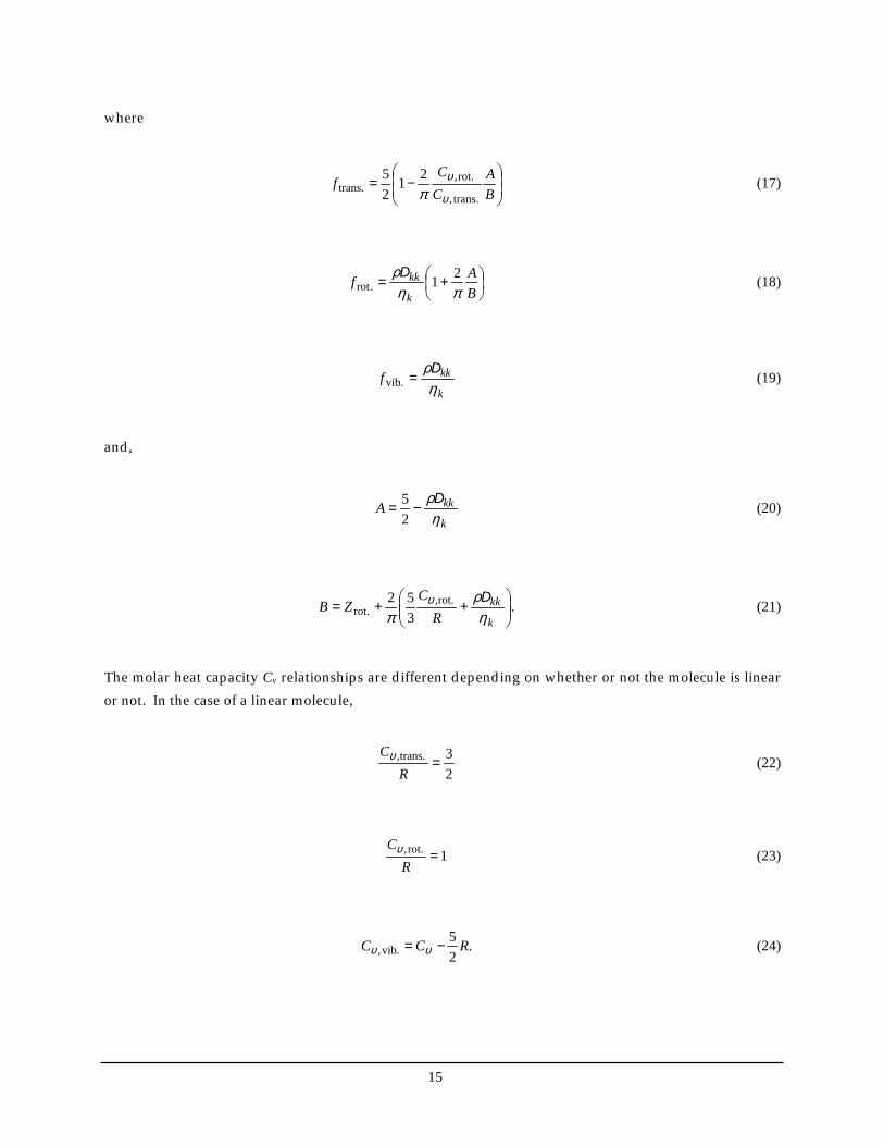
where

−=

BA

CC

ftrans.,

.rot,trans.

2125

υ

υπ

(17)

+=BAf

k

kkπη

ρ 21.rotD

(18)

k

kkfη

ρD=vib. (19)

and,

k

kkAη

ρD−=

25 (20)

.352 .rot,

.rot

++=

k

kkR

CZB

ηρ

πυ D (21)

The molar heat capacity Cv relationships are different depending on whether or not the molecule is linear or not. In the case of a linear molecule,

23trans., =

RCυ (22)

1rot., =R

Cυ (23)

.25

vib., RCC −= υυ (24)

16

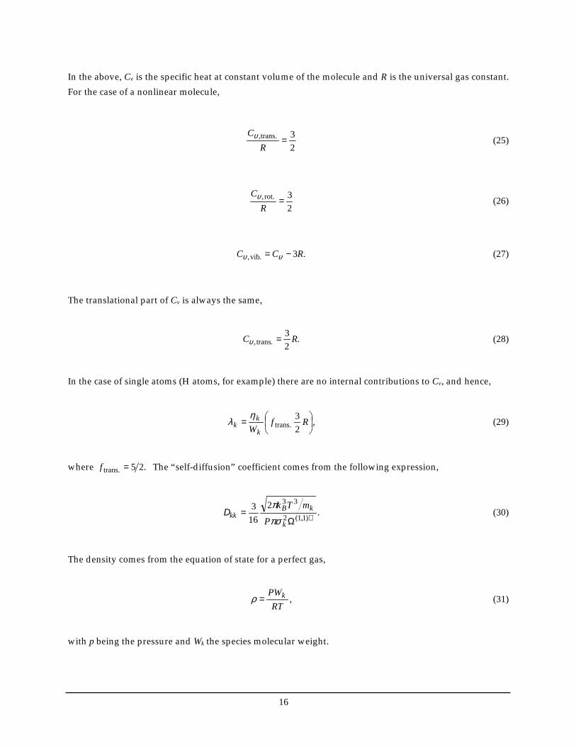
In the above, Cv is the specific heat at constant volume of the molecule and R is the universal gas constant. For the case of a nonlinear molecule,

23trans., =

RCυ (25)

23.rot, =

RCυ (26)

.3.vib, RCC −= υυ (27)

The translational part of Cv is always the same,

.23

.trans, RC =υ (28)

In the case of single atoms (H atoms, for example) there are no internal contributions to Cv, and hence,

,23

trans.

= RfWk

kk

ηλ (29)

where .25trans. =f The “self-diffusion” coefficient comes from the following expression,

.2

163

)1,1(2

33

∗Ω=

k

kBkk

P

mTk

πσ

πD (30)

The density comes from the equation of state for a perfect gas,

,RT

PWk=ρ (31)

with p being the pressure and Wk the species molecular weight.

17

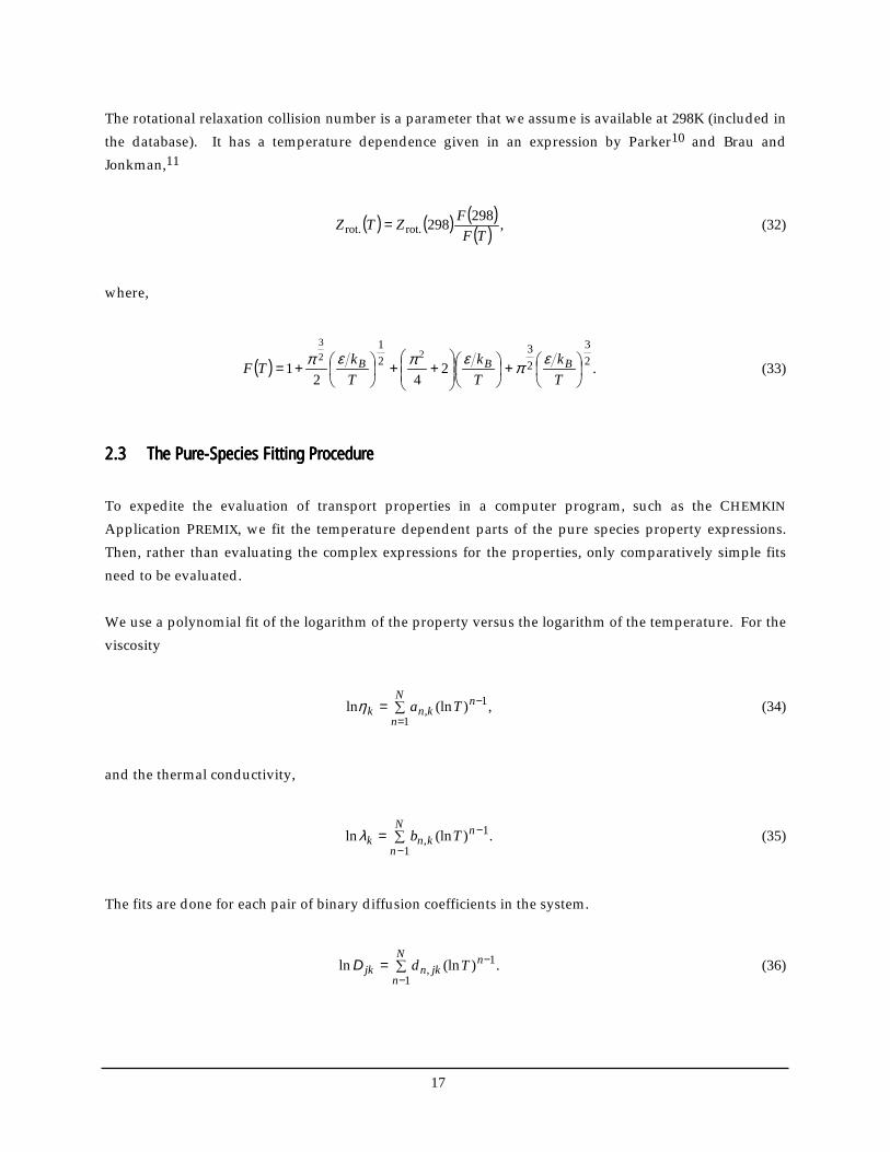
The rotational relaxation collision number is a parameter that we assume is available at 298K (included in the database). It has a temperature dependence given in an expression by Parker10 and Brau and Jonkman,11

( ) ( ) ( )( ) ,298298rot.rot. TF

FZTZ = (32)

where,

( ) .242

1 23

23

21

223

+

++

+=Tk

Tk

TkTF BBB επεπεπ (33)

2.32.32.32.3 The PureThe PureThe PureThe Pure----Species Fitting ProcedureSpecies Fitting ProcedureSpecies Fitting ProcedureSpecies Fitting Procedure

To expedite the evaluation of transport properties in a computer program, such as the CHEMKIN Application PREMIX, we fit the temperature dependent parts of the pure species property expressions. Then, rather than evaluating the complex expressions for the properties, only comparatively simple fits need to be evaluated. We use a polynomial fit of the logarithm of the property versus the logarithm of the temperature. For the viscosity

,)(lnln1

1,=

=

−N

n

nknk Taη (34)

and the thermal conductivity,

.)(lnln1

1,=

−

−N

n

nknk Tbλ (35)

The fits are done for each pair of binary diffusion coefficients in the system.

.)(lnln1

1,=

−

−N

n

njknjk TdD (36)

18

By default TRANSPORT uses third- order polynomial fits (i.e., N = 4) and we find that the fitting errors are well within one percent. The fitting procedure must be carried out for the particular system of gases that is present in a given problem. Therefore, the fitting cannot be done “once and for all,” but must be done once at the beginning of each new problem. The viscosity and conductivity are independent of pressure, but the diffusion coefficients depend inversely on pressure. The diffusion coefficient fits are computed at unit pressure; the later evaluation of a diffusion coefficient is obtained by simply dividing the diffusion coefficient as evaluated from the fit by the actual pressure. Even though the single component conductivities are fit and passed to the TRANSPORT Subroutine Library, they are not used in the computation of multicomponent thermal conductivities; they are used only for the evaluation of the mixture-averaged conductivities.

2.42.42.42.4 The Mass, Momentum, and Energy FluxesThe Mass, Momentum, and Energy FluxesThe Mass, Momentum, and Energy FluxesThe Mass, Momentum, and Energy Fluxes

The momentum flux is related to the gas mixture viscosity and the velocities by

( )( ) ( )δυκηυυητ ⋅∇

−+∇+∇−=32T , (37)

where υ is the velocity vector, ( )υ∇ is the dyadic product, ( )Tυ∇ is the transpose of the dyadic product, and δδδδ is the unit tensor.5 In the TRANSPORT software package we provide average values for the mixture viscosity η, but we do not provide information on the bulk viscosity κ. The energy flux is given in terms of the thermal conductivity λ 0 by

,11

0 ==

−∇−=K

kk

Tk

kk

K

kkk D

XWRTTh djq λ (38)

where,

( ) .1 pp

YXX kkkk ∇−+∇=d (39)

The multicomponent species flux is given by

19

,kkk Y Vj ρ= (40)

where Yk are the mass fractions and the diffusion velocities are given by

.11, T

TD

DWWX k

Tk

K

kjjjkj

kk ∇−=

≠ YdV

ρ (41)

The species molar masses are denoted by Wk and the mean molar mass byW . jkD , are the ordinary multicomponent diffusion coefficients, and T

kD are the thermal diffusion coefficients. By definition in the mixture-average formulations, the diffusion velocity is related to the species gradients by a Fickian formula as,

.11 TTY

DD

X k

Tk

kkmk

k ∇−−=ρ

dV (42)

The mixture diffusion coefficient for species k is computed as 5

−=

≠K

kj jkj

kkm X

YD

D1 (43)

A potential problem with this expression is that it is not mathematically well defined in the limit of the mixture becoming a pure species. Even though diffusion itself has no real meaning in the case of a pure species, the numerical implementation must ensure that the diffusion coefficients behave reasonably and that the program does not “blow up” when the pure species condition is reached. We circumvent these problems by evaluating the diffusion coefficients in the following equivalent way.

≠

≠= Kkj jkj

Kkj jj

kmXW

WXD

D (44)

In this form the roundoff is accumulated in roughly the same way in both the numerator and denominator, and thus the quotient is well behaved as the pure species limit is approached. However, if the mixture is exactly a pure species, the formula is still undefined.

20

To overcome this difficulty we always retain a small quantity of each species. In other words, for the purposes of computing mixture diffusion coefficients, we simply do not allow a pure species situation to occur; we always maintain a residual amount of each species. Specifically, we assume in the above formulas that

,ˆ δ+= kk XX (45)

where ˆ X k is the actual mole fraction and δ is a small number that is numerically insignificant compared to any mole fraction of interest, yet which is large enough that there is no trouble representing it on any computer. A value of 10-12 for δ works well. In some cases (for example, Warnatz12 and Coltrin et al.13) it can be useful to treat multicomponent diffusion in terms of an equivalent Fickian diffusion process. This is sometimes a programming convenience in that the computer data structure for the multicomponent process can be made to look like a Fickian process. To do so supposes that a mixture diffusion coefficient can be defined in such a way that the diffusion velocity is written as Eq. (42) rather than Eq. (41). This equivalent Fickian diffusion coefficient is then derived by equating Eq. (41) and (42) and solving for Dkm as

k

Kkj jjkj

km W

DWD

d

d ≠−=,

(46)

Unfortunately, this equation is undefined as the mixture approaches a pure species condition. To help deal with this difficulty a small number (ε =10−12 ) may be added to both the numerator and denominator to obtain

)( ε

ε

+

+−= ≠

k

Kkj jkjj

km W

DWD

d

d

Furthermore, for the purposes of evaluating the “multicomponent” Dkm, it may be advantageous to compute the dk in the denominator using the fact that ∇−=∇ ≠

Kkj jk XX . In this way the summations in

the numerator and the denominator accumulate any rounding errors in roughly the same way, and thus the quotient is more likely to be well behaved as the pure species limit is approached. Since there is no diffusion due to species gradients in a pure species situation, the exact value of the diffusion coefficient is not as important as the need for is simply to be well defined, and thus not cause computational difficulties.

21

In practice we have found mixed results using the equivalent Fickian diffusion to represent multicomponent processes. In some marching or parabolic problems, such as boundary layer flow in channels,13 we find that the equivalent Fickian formulation is preferable. However, in some steady state boundary value problems, we have found that the equivalent Fickian formulation fails to converge, whereas the regular multicomponent formulation works quite well. Thus, we cannot confidently recommend which formulation should be preferred for any given application.

2.52.52.52.5 The MixtureThe MixtureThe MixtureThe Mixture----Averaged PropertiesAveraged PropertiesAveraged PropertiesAveraged Properties

Our objective in this section is to determine mixture properties from the pure species properties. In the case of viscosity, we use the semi-empirical formula due to Wilke14 and modified by Bird et al.5 The Wilke formula for mixture viscosity is given by

Φ

== =

K

k Kj kjj

kkX

X1 1

ηη (48)

where,

.118

1

2

41

21

21

+

+=Φ

−

k

j

j

k

j

kkj W

WWW

ηη

(49)

For the mixture-averaged thermal conductivity we use a combination averaging formula15

+=

= =

K

k Kk kk

kk XX

1 1

121

λλλ (50)

2.62.62.62.6 Thermal Diffusion RatiosThermal Diffusion RatiosThermal Diffusion RatiosThermal Diffusion Ratios

The thermal diffusion coefficients are evaluated in the following section on multicomponent properties. This section describes a relatively inexpensive way to estimate the thermal diffusion of light species into a mixture. This is the method that is used in our previous transport package, and it is included here for the sake of upward compatibility. This approximate method is considerably less accurate than the thermal diffusion coefficients that are computed from the multicomponent formulation.

22

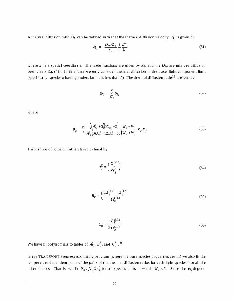
A thermal diffusion ratio Θk can be defined such that the thermal diffusion velocity kW is given by

ik

kkmk x

TTX

Di ∂

∂1Θ−=W (51)

where xi is a spatial coordinate. The mole fractions are given by Xk, and the Dkm are mixture diffusion coefficients Eq. (42). In this form we only consider thermal diffusion in the trace, light component limit (specifically, species k having molecular mass less than 5). The thermal diffusion ratio16 is given by

=Θ≠

K

kjkjk θ (52)

where

( )( )( ) jk

jk

jk

kjkjkj

kjkjkj XX

WWWW

BAA

CA+−

+−

−+=

∗∗∗

∗∗

551216

56522

15θ (53)

Three ratios of collision integrals are defined by

)1,1(

)2,2(

21

ij

ijijA

Ω

Ω=∗ (54)

),11(

)3,1()2,1(5

31

ij

ijijijB

Ω

Ω−Ω=∗ (55)

)1,1(

)2,1(

31

ij

ijijC

Ω

Ω=∗ (56)

We have fit polynomials to tables of *

ijA , *ijB , and *

ijC . 8 In the TRANSPORT Preprocessor fitting program (where the pure species properties are fit) we also fit the temperature dependent parts of the pairs of the thermal diffusion ratios for each light species into all the other species. That is, we fit ( )kjkj XXθ for all species pairs in which 5<kW . Since the kjθ depend

23

weakly on temperature, we fit to polynomials in temperature, rather than the logarithm of temperature. The coefficients of these fits are written onto the Linking File.

2.72.72.72.7 The Multicomponent PropertiesThe Multicomponent PropertiesThe Multicomponent PropertiesThe Multicomponent Properties

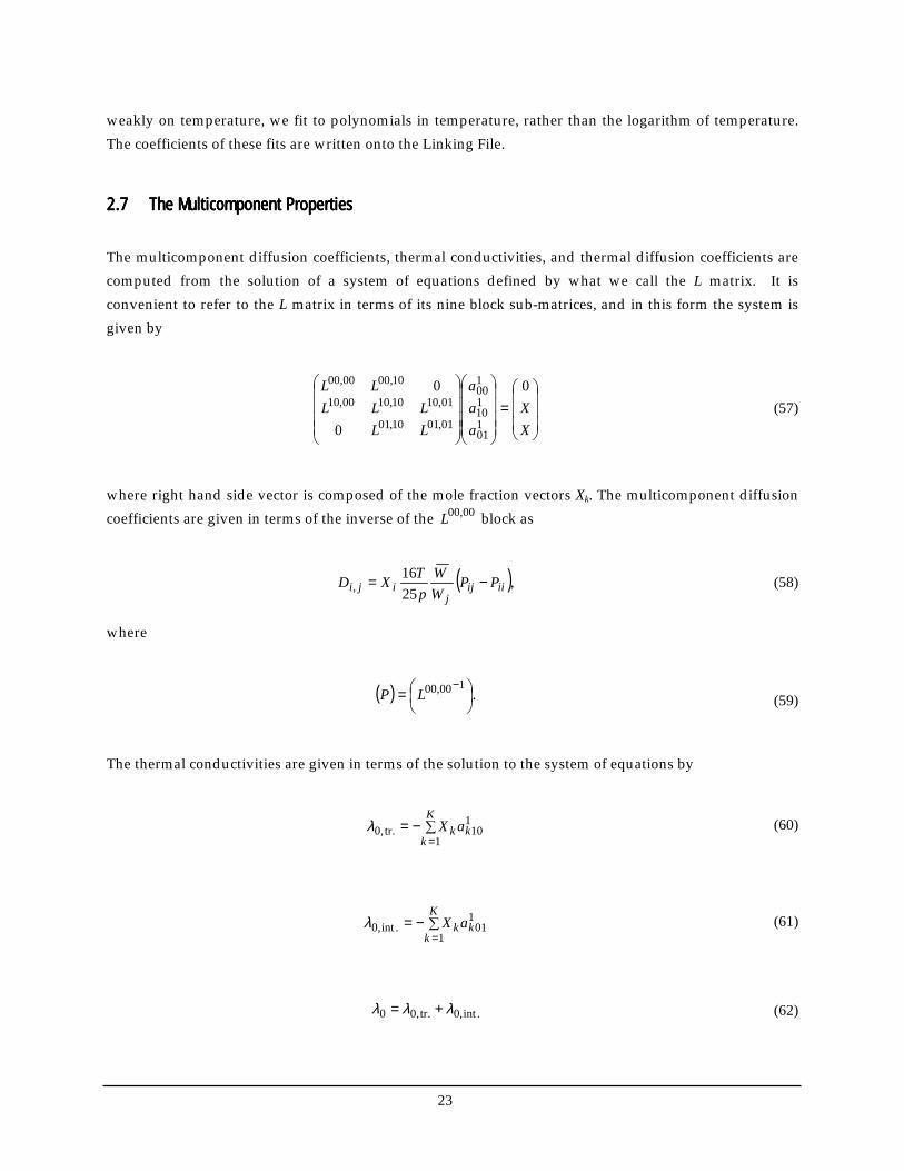
The multicomponent diffusion coefficients, thermal conductivities, and thermal diffusion coefficients are computed from the solution of a system of equations defined by what we call the L matrix. It is convenient to refer to the L matrix in terms of its nine block sub-matrices, and in this form the system is given by

=

XX

aaa

LLLLL

LL 0

0

0

101

110

100

01,0110,01

01,1010,1000,10

10,0000,00

(57)

where right hand side vector is composed of the mole fraction vectors Xk. The multicomponent diffusion coefficients are given in terms of the inverse of the L00,00 block as

( ),2516

, iiijj

iji PPWW

pTXD −= (58)

where

( ) .100,00

=−

LP (59)

The thermal conductivities are given in terms of the solution to the system of equations by

−==

K

kkk aX

1

110.tr,0λ (60)

−==

K

kkk aX

1

101.int,0λ (61)

.int,0.tr,00 λλλ += (62)

24

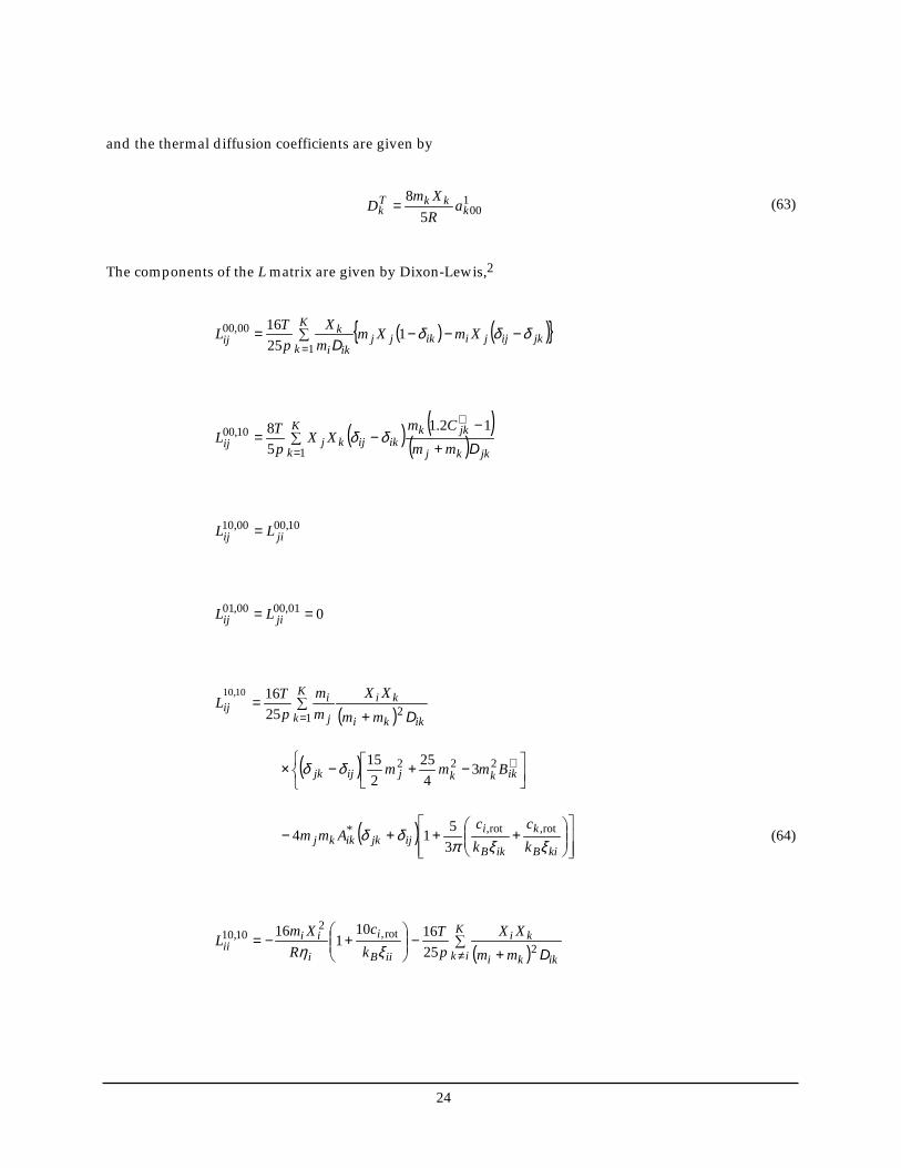
and the thermal diffusion coefficients are given by

1005

8k

kkTk a

RXm

D = (63)

The components of the L matrix are given by Dixon-Lewis,2

( ) ( ) jkijjiikjjK

k iki

kij XmXm

mX

pTL δδδ −−−=

=1

2516

1

00,00D

( ) ( )( ) jkkj

jkkikij

K

kkjij mm

CmXX

pTL

D+−

−=∗

=

12.158

1

10,00 δδ

10,0000,10jiij LL =

001,0000,01 == jiij LL

( ) ikki

kiK

k j

iij

mmXX

mm

pTL

D21251610,10

+==

( )

−+−× ∗ikkkjijjk Bmmm 222 3

425

215 δδ

( )

+++−

kiB

k

ikB

iijjkikkj k

ckc

Ammξξπ

δδ rot,rot,*3514 (64)

( )

+

−

+−=

≠

K

ik ikki

ki

iiB

i

i

iiii mm

XXpT

kc

RXmL

D2rot,

210,10

251610

116

ξη

25

+−+× ∗∗

ikkiikkki AmmBmmm 43425

215 222

++×

kiB

k

ikB

ikc

kc

ξξπrot,rot,

351

( ) ( ) ++

==

∗K

k jkB

jkjijik

jkkj

jkj

jij k

cXX

mmAm

pcTL

1

rot,

int,

01,105

32ξ

δδπ D

iiB

i

ii

Biiii k

c

cRkXm

Lξηπint,

int,

201,10

316=

( ) ikB

ikj

K

ik jkki

iki

i

Bkc

XXmmAm

pcTk

ξπrot,

int,532

+

+≠

∗

D

01,1010,01jiij LL =

iiB

i

i

ii

i

Bii k

cR

XmckL

ξηπrot,

2

2int,

210,01 8

−=

+−≠

∗

=

K

ik ii

i

ik

ik

k

i

i

kiK

k ki

ki

i

B cAmm

cXX

DXX

pcTk

ξπrot.

.int 1 ,int. .int, 5124

D

( )jiLij ≠= 001,01

26

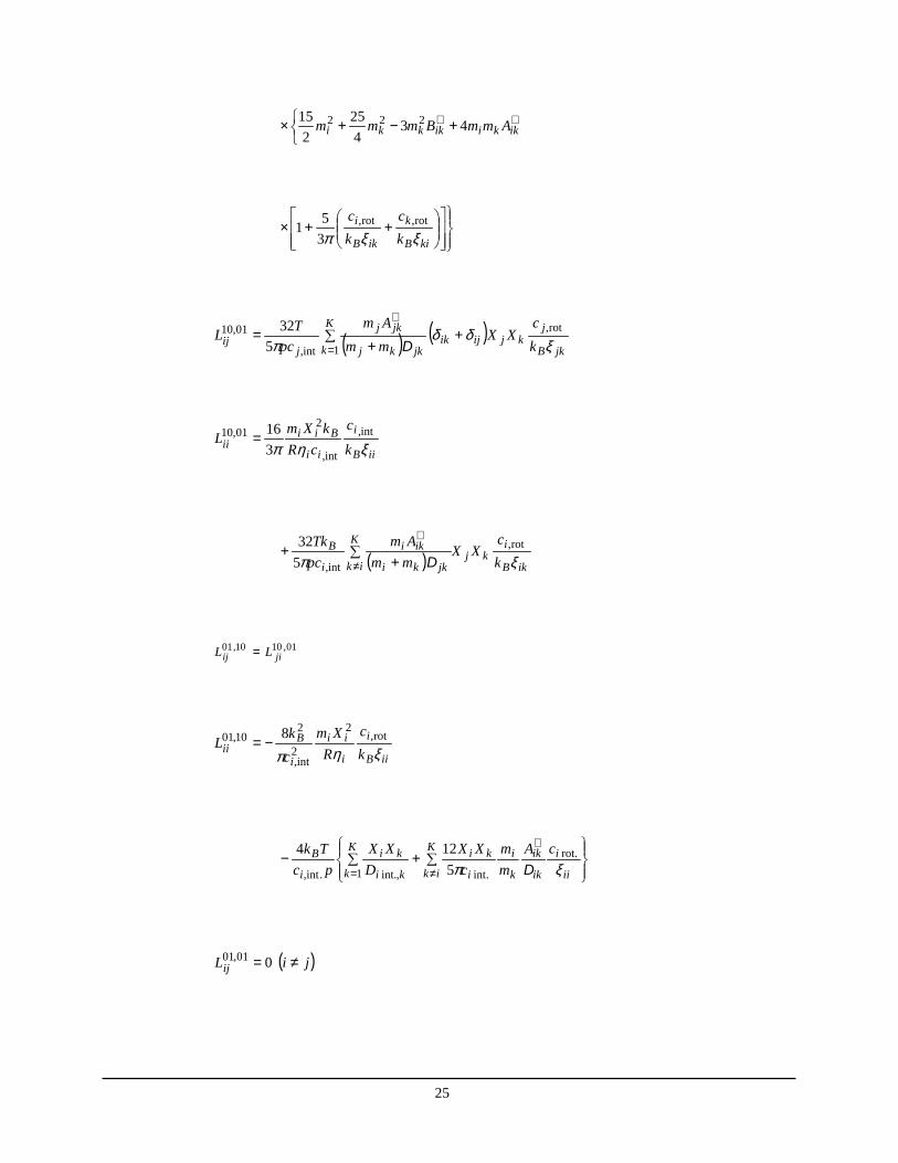
In these equations T is the temperature, p is the pressure, Xk is the mole fraction of species k, ikD are the binary diffusion coefficients, and mi is the molecular mass of species i. Three ratios of collision integrals ∗

jkA , ∗jkB , and ∗

jkC are defined by Eqs. (54-56). The universal gas constant is represented by R and the pure species viscosities are given as kη . The rotational and internal parts of the species molecular heat capacities are represented by rot,kc and ck,int . For a linear molecule

,1rot, =B

k

kc

(65)

and for a nonlinear molecule

.23rot, =

B

k

kc

(66)

The internal component of heat capacity is computed by subtracting the translational part from the full heat capacity as evaluated from the CHEMKIN Thermodynamic Database.

.23int, −=

B

p

B

k

kc

kc

(67)

Following Dixon-Lewis,2 we assume that the relaxation collision numbers ijξ depend only on the species i, i.e., all iiij ξξ = . The rotational relaxation collision number at 298K is one of the parameters in the transport database, and its temperature dependence was given in Eqs. (32) and (33). For non-polar gases the binary diffusion coefficients for internal energy ki int., D are approximated by the ordinary binary diffusion coefficients. However, in the case of collisions between polar molecules, where the exchange is energetically resonant, a large correction of the following form is necessary,

( ) ,1,int

pp

pppp δ ′+

=D

D (68)

where,

3

2985

Tpp =′δ (69)

when the temperature is in Kelvins.

27

There are some special cases that require modification of the L matrix. First, for mixtures containing monatomic gases, the rows that refer to the monatomic components in the lower block row and the corresponding columns in the last block column must be omitted. That this required is clear by noting that the internal part of the heat capacity appears in the denominator of terms in these rows and columns (e.g., Lij

10,01 ). An additional problem arises as a pure species situation is approached, because all Xk except one approach zero, and this causes the L matrix to become singular. Therefore, for the purposes of forming L we do not allow a pure species situation to occur. We always retain a residual amount of each species by computing the mole fractions from

δ+=k

kk W

YWX (70)

A value of δ = 10−12 works well; it is small enough to be numerically insignificant compared to any mole fraction of interest, yet it is large enough to be represented on nearly any computer.

2.82.82.82.8 Species ConservationSpecies ConservationSpecies ConservationSpecies Conservation

Some care needs to be taken in using the mixture-averaged diffusion coefficients as described here. The mixture formulas are approximations, and they are not constrained to require that the net species diffusion flux is zero, i.e., the condition.

=K

kkkY

10

=V (71)

need not be satisfied. Therefore, one must expect that applying these mixture diffusion relationships in the solution of a system of species conservation equations should lead to some nonconservation, i.e., the resultant mass fractions will not sum to one. Therefore, one of a number of corrective actions must be invoked to ensure mass conservation. Unfortunately, resolution of the conservation problem requires knowledge of species flux, and hence details of the specific problem and discretization method. Therefore, it is not reasonable in the general setting of the present software package to attempt to enforce conservation. Nevertheless, the user of the package must be aware of the difficulty, and consider its resolution when setting up the difference approximations to his particular system of conservation equations. One attractive method is to define a “conservation diffusion velocity” as Coffee and Heimerl6 recommend. In this approach we assume that the diffusion velocity vector is given as

28

,ˆ ckk VVV += (72)

where ˆ V k is the ordinary diffusion velocity Eq. (42) and Vc is a constant correction factor (independent of species, but spatially varying) introduced to satisfy Eq. (71). The correction velocity is defined by

.ˆ1

−==

K

kkkc Y VV (73)

This approach is the one followed by Miller et al.17-19 in their flame models. An alternative approach is attractive in problems having one species that is always present in excess. Here, rather than solving a conservation equation for the one excess species, its mass fraction is computed simply by subtracting the sum of the remaining mass fractions from unity. A similar approach involves determining locally at each computational cell which species is in excess. The diffusion velocity for that species is computed to require satisfaction of Eq. (71). Even though the multicomponent formulation is theoretically forced to conserve mass, the numerical implementations can cause some slight nonconservation. Depending on the numerical method, even slight inconsistencies can lead to difficulties. Methods that do a good job of controlling numerical errors, such as the differential/algebraic equation solver DASSL (Petzold, 1982), are especially sensitive to inconsistencies, and can suffer computational inefficiencies or convergence failures. Therefore, even when the multicomponent formulation is used, it is often advisable to provide corrective measures such as those described above for the mixture-averaged approach. However, the magnitude of any such corrections will be significantly smaller.

29

3.3.3.3. THE MECHANICS OF USING THE PACKAGETHE MECHANICS OF USING THE PACKAGETHE MECHANICS OF USING THE PACKAGETHE MECHANICS OF USING THE PACKAGE

3.13.13.13.1 General FlGeneral FlGeneral FlGeneral Flow of Informationow of Informationow of Informationow of Information The TRANSPORT package must be used in conjunction with the CHEMKIN Gas-phase Utility package. The general flow of information is depicted in Figure 1. The first step is to execute the CHEMKIN Interpreter. The gas-phase CHEMKIN kinetics package is documented separately in the CHEMKIN Gas-phase Utility user’s manual. The CHEMKIN Interpreter first reads user-supplied information about the species and chemical reactions in a problem. It then extracts further information about the species’ thermodynamic properties from the Thermodynamics Database and from a separate user input file, if provided. This information is stored on the CHEMKIN Linking File, a file that is needed by the TRANSPORT Property Fitting routine, and later by the CHEMKIN Gas-Phase Subroutine Library. The next program to be executed is the TRANSPORT Property Fitting routine. It needs input from the TRANSPORT Property Database, and from the CHEMKIN Linking File. The TRANSPORT database contains molecular parameters for a number of species; these parameters are: The Lennard-Jones well depth Bkε in Kelvins, the Lennard-Jones collision diameter σ in Angstroms, the dipole moment µ in Debyes, the polarizability α in cubic angstroms, the rotational relaxation collision number Zrot and an indicator regarding the nature and geometrical configuration of the molecule. A supplemental input file can also contain this information, as described in Section 3.3 below. The information coming from the CHEMKIN Linking File contains the species names. The names in both the CHEMKIN and the TRANSPORT databases must correspond exactly. Like the CHEMKIN Interpreter, the TRANSPORT Fitting routine produces a TRANSPORT Linking File that is later needed in the TRANSPORT Property Subroutine Library.

3.23.23.23.2 Accessing the Transport Property Subroutine Library from an ApplicationAccessing the Transport Property Subroutine Library from an ApplicationAccessing the Transport Property Subroutine Library from an ApplicationAccessing the Transport Property Subroutine Library from an Application Both the CHEMKIN and the TRANSPORT subroutine libraries must be initialized before use and there is a similar initialization subroutine in each. The TRANSPORT Subroutine Library is initialized by a call to subroutine MCINIT. Its purpose is to read the TRANSPORT Linking File and set up the internal working and storage space that must be made available to all other subroutines in the library. Once initialized, any subroutine in the library may be called from the application programs.

30

Gas-PhaseChemistry

CHEMKINLink File

CHEMKINLibrary

TRANSPORTLibrary

TRANSPORTLink File

TRANSPORTFitting Program

TransportTransportTransportTransport

Gas Phase ChemistryGas Phase ChemistryGas Phase ChemistryGas Phase Chemistry

CCCCHEMKIN HEMKIN HEMKIN HEMKIN AAAAPPLICATIONPPLICATIONPPLICATIONPPLICATION Text Output

CHEMKINInterpreter

ThermodynamicData

TransportData

APPLICATION Input

Figure 1. Schematic representing the relationship of the TRANSPORT package,

CHEMKIN, and the Application program.

3.33.33.33.3 Use of CommandUse of CommandUse of CommandUse of Command----Line ArgumentsLine ArgumentsLine ArgumentsLine Arguments As an alternative or supplement to the Transport Database file, a separate input file may be specified on the command-line when the Transport Property Fitting routine is invoked. In fact, all input file names can be specified on the command-line. An example is shown in Figure 2. Here the command-line argument “-i” indicates the next string is the name of the supplemental transport input file. Similarly, -o is the diagnostic output file, -c is the Chemkin Linking File, -d is the Transport Property Database file, and –t is the output Transport Property Linking File. Full pathnames are needed for the files only if they are not located in the user’s working directory.

tran –i tran.inp –o tran.out –c chem.asc –d tran.dat –t tran.asc

Figure 2. Example Use of Command-line Arguments for the TRANSPORT program.

31

4.4.4.4. QUICK REFERENCE TO THE TRANSPORT SUBROUTINE LIBRARYQUICK REFERENCE TO THE TRANSPORT SUBROUTINE LIBRARYQUICK REFERENCE TO THE TRANSPORT SUBROUTINE LIBRARYQUICK REFERENCE TO THE TRANSPORT SUBROUTINE LIBRARY This chapter is arranged by topical area to provide a quick reference to each of the TRANSPORT Library Subroutines. In addition to the subroutine call list itself, the purpose of the subroutine is briefly described.

4.14.14.14.1 MnemonicsMnemonicsMnemonicsMnemonics

There are seventeen user-callable subroutines in the package. All subroutine names begin with MC. The following letter is either an S and A or an M, indicating whether pure species (S), mixture-averaged (A), or multicomponent (M) properties are returned. The remaining letters indicate which property is returned: CON for conductivity, VIS for viscosity, DIF for diffusion coefficients, CDT for both conductivity and thermal diffusion coefficients, and TDR for the thermal diffusion ratios. A call to the initialization subroutine MCINIT must precede any other call. This subroutine is normally called only once at the beginning of a problem; it reads the Linking File and sets up the internal storage and working space - arrays IMCWRK and RMCWRK. These arrays are required input to all other subroutines in the library. Besides MCINIT there is only one other non-property subroutine, called MCPRAM; it is used to return the arrays of molecular parameters that came from the database for the species in the problem. All other subroutines are used to compute either viscosities, thermal conductivities, or diffusion coefficients. They may be called to return pure species properties, mixture-averaged properties, or multicomponent properties. In the input to all subroutines, the state of the gas is specified by the pressure in dynes per square centimeter, temperature in Kelvins, and the species mole fractions. The properties are returned in standard CGS units. The order of vector information, such as the vector of mole fractions or pure species viscosities, is the same as the order declared in the CHEMKIN Interpreter input. Here we provide a short description of each subroutine according to its function. In Chaper 5 we list the subroutines in alphabetical order and provide a longer description of each subroutine including call-list details.

32

4.24.24.24.2 Initialization and ParametersInitialization and ParametersInitialization and ParametersInitialization and Parameters

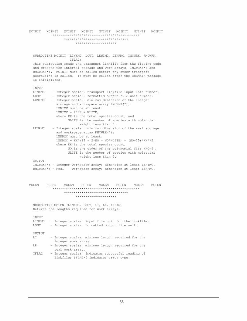
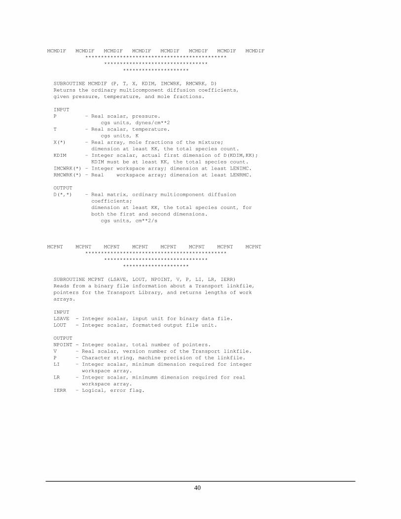
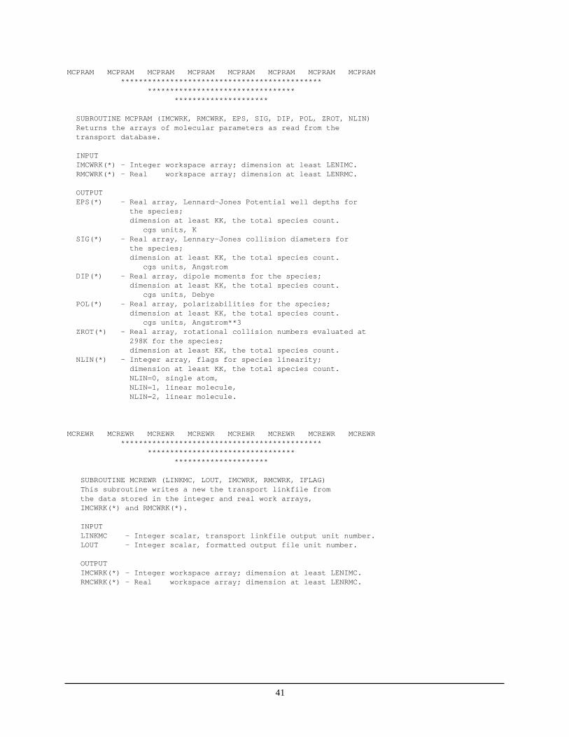
SUBROUTINE MCINIT (LINKMC, LOUT, LENIMC, LENRMC, IMCWRK, RMCWRK) This subroutine serves to read the Linking File from the fitting code and to create the internal storage and work arrays, IMCWRK(*) and RMCWRK (*). MCINIT must be called before any other transport subroutine is called. It must be called after the CHEMKIN package is initialized. SUBROUTINE MCPRAM (IMCWRK, RMCWRK EPS, SIG, DIP, POL, ZROT, NLIN) This subroutine is called to return the arrays of molecular parameters as read from the transport database. SUBROUTINE MCPNT (LSAVE, LOUT, NPOINT, V, P, LI, LR, IERR) Reads from a binary file information about a TRANSPORT linkfile, pointers for the TRANSPORT Library, and returns lengths of work arrays. SUBROUTINE MCSAVE (LOUT, LSAVE, IMCWRK, RMCWRK) Writes to a binary file information about a TRANSPORT linkfile, pointers for the TRANSPORT library, and TRANSPORT work arrays. SUBROUTINE MCREWR (LINKMC, LOUT, IMCWRK, RMCWRK, IFLAG) This subroutine writes a new the transport linkfile from the data stored in the integer and real work arrays, IMCWRK(*) and RMCWRK(*).

4.34.34.34.3 ViscosityViscosityViscosityViscosity

SUBROUTINE MCSVIS (T, RMCWRK, VIS) This subroutine computes the array of pure species viscosities given the temperature. SUBROUTINE MCAVIS (T, X, RMCWRK, VISMIX) This subroutine computes the mixture viscosity given the temperature and the species mole fractions. It uses modifications of the Wilke semi-empirical formulas. SUBROUTINE MCCVEX (K, KDIM, RCKWRK, COFVIS) Gets or puts values of the fitting coefficients for the polynomial fits to species viscosity.

33

4.44.44.44.4 ConductivityConductivityConductivityConductivity

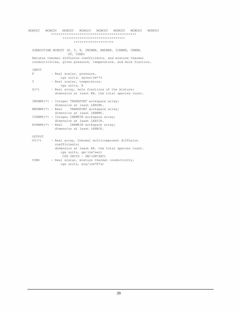
SUBROUTINE MCSCON (T, RMCWRK, CON) This subroutine computes the array pure species conductivities given the temperature. SUBROUTINE MCACON (T, X, RMCWRK, CONMIX) This subroutine computes the mixture thermal conductivity given the temperature and the species mole fractions. SUBROUTINE MCMCDT (P, T, X, IMCWRK, RMCWRK, ICKWRK, CKWRK, DT, COND) This subroutine computes the thermal diffusion coefficients and mixture thermal conductivities given the pressure, temperature, and mole fractions. SUBROUTINE MCCCEX (K, KDIM, RCKWRK, COFCON) Gets or puts values of the fitting coefficients for the polynomial fits to species conductivity.

4.54.54.54.5 Diffusion CDiffusion CDiffusion CDiffusion Coefficientsoefficientsoefficientsoefficients

SUBROUTINE MCSDIF (P, T, KDIM, RMCWRK, DJK) This subroutine computes the binary diffusion coefficients given the pressure and temperature. SUBROUTINE MCADIF (P, T, X, RMCWRK, D) This subroutine computes the mixture-averaged diffusion coefficients given the pressure, temperature, and species mole fractions. SUBROUTINE MCMDIF (P, T, X, KDIM, IMCWRK, RMCWRK, D) This subroutine computes the ordinary multicomponent diffusion coefficients given the pressure, temperature, and mole fractions. SUBROUTINE MCCDEX (K, KDIM, RCKWRK, COFDIF) Gets or puts values of the fitting coefficients for the polynomial fits to species binary diffusion coefficients.

4.64.64.64.6 Thermal DiffusionThermal DiffusionThermal DiffusionThermal Diffusion

SUBROUTINE MCATDR (T, X, IMCWRK, RMCWRK, TDR) This subroutine computes the thermal diffusion ratios for the light species into the mixture.

34

SUBROUTINE MCMCDT (P, T, X, IMCWRK, RMCWRK, ICKWRK, CKWRK, DT, COND) This subroutine computes the thermal diffusion coefficients, and mixture thermal conductivities given the pressure, temperature, and mole fractions.

35

5.5.5.5. ALPHABETICAL LISTING OF THE TRANSPORT SUBROUTINE LIBRARY WITH ALPHABETICAL LISTING OF THE TRANSPORT SUBROUTINE LIBRARY WITH ALPHABETICAL LISTING OF THE TRANSPORT SUBROUTINE LIBRARY WITH ALPHABETICAL LISTING OF THE TRANSPORT SUBROUTINE LIBRARY WITH DETAILED DESCRIPTIONS OF THE CALL LISTSDETAILED DESCRIPTIONS OF THE CALL LISTSDETAILED DESCRIPTIONS OF THE CALL LISTSDETAILED DESCRIPTIONS OF THE CALL LISTS

The following pages list detailed descriptions for the user interface to each of the package’s seventeen user-callable subroutines. They are listed in alphabetical order. MCACON MCACON MCACON MCACON MCACON MCACON MCACON MCACON

******************************************************************************

*********************

SUBROUTINE MCACON (T, X, RMCWRK, CONMIX)Returns the mixture thermal conductivity given temperature andspecies mole fractions.

INPUTT - Real scalar, temperature.

cgs units, KX(*) - Real array, mole fractions of the mixture;

dimension at least KK, the total species count.RMCWRK(*) - Real workspace array; dimension at least LENRMC.

OUTPUTCONMIX - Real scalar, mixture thermal conductivity.

cgs units, erg/cm*K*s

MCADIF MCADIF MCADIF MCADIF MCADIF MCADIF MCADIF MCADIF*********************************************

******************************************************

SUBROUTINE MCADIF (P, T, X, RMCWRK, D)Returns mixture-averaged diffusion coefficients given pressure,temperature, and species mole fractions.

INPUTP - Real scalar, pressure.

cgs units, dynes/cm**2T - Real scalar, temperature.



OUTPUTD(*) - Real array, mixture diffusion coefficients;

dimension at least KK, the total species count.cgs units, cm**2/s

36

MCAVIS MCAVIS MCAVIS MCAVIS MCAVIS MCAVIS MCAVIS MCAVIS*********************************************

******************************************************

SUBROUTINE MCAVIS (T, X, RMCWRK, VISMIX)Returns mixture viscosity, given temperature and species molefractions. It uses modification of the Wilke semi-empiricalformulas.




OUTPUTVISMIX - Real scalar, mixture viscosity.

cgs units, gm/cm*s

MCCCEX MCCCEX MCCCEX MCCCEX MCCCEX MCCCEX MCCCEX MCCCEX*********************************************

******************************************************

SUBROUTINE MCCCEX (K, KDIM, RCKWRK, COFCON)Gets or puts values of the fitting coefficients for thepolynomial fits to species conductivity.

INPUTK - Integer scalar, species index.

K > 0 gets coefficients from RMCWRKK < 0 puts coefficients into RMCWRK

KDIM - Dimension for COFCON - the total number of speciesRMCWRK(*) - Real workspace array; dimension at least LENRMC.

If K < 1:COFCON - Real vector of polynomial coefficients for

the species' conductivity; dimension at least NO,usually 4.

OUTPUTIf K > 1:COFCON - Real vector of polynomial coefficients for

the species' conductivity; dimension at least NO,usually 4.

37

MCCDEX MCCDEX MCCDEX MCCDEX MCCDEX MCCDEX MCCDEX MCCDEX*********************************************

******************************************************

SUBROUTINE MCCDEX (K, KDIM, RCKWRK, COFDIF)Gets or puts values of the fitting coefficients for thepolynomial fits to species binary diffusion coefficients.



KDIM - Dimension for COFDIF - the total number of speciesRMCWRK(*) - Real workspace array; dimension at least LENRMC.

If K < 1:COFDIF - Real matrix of polynomial coefficients for

the species' binary diffusion coefficient with allother species; The first dimension should be KK;the second dimension should be NO, usually 4;

OUTPUTIf K > 1:COFDIF - Real matrix of polynomial coefficients for

the species' binary diffusion coefficient with allother species; first dimension should be NO, usually 4;The second dimension should be NKK

MCCVEX MCCVEX MCCVEX MCCVEX MCCVEX MCCVEX MCCVEX MCCVEX*********************************************

******************************************************

SUBROUTINE MCCVEX (K, KDIM, RCKWRK, COFVIS)Gets or puts values of the fitting coefficients for thepolynomial fits to species viscosity.



KDIM - Dimension for COFVIS - the total number of speciesRMCWRK(*) - Real workspace array; dimension at least LENRMC.

If K < 1:COFVIS - Real vector of polynomial coefficients for

the species' viscosity; dimension at least NO, usually 4

OUTPUTIf K > 1:COFVIS - Real vector of polynomial coefficients; dimension

at least NO, usually = 4

38

MCINIT MCINIT MCINIT MCINIT MCINIT MCINIT MCINIT MCINIT*********************************************

******************************************************

SUBROUTINE MCINIT (LINKMC, LOUT, LENIMC, LENRMC, IMCWRK, RMCWRK,IFLAG)

This subroutine reads the transport linkfile from the fitting codeand creates the internal storage and work arrays, IMCWRK(*) andRMCWRK(*). MCINIT must be called before any other transportsubroutine is called. It must be called after the CHEMKIN packageis initialized.

INPUTLINKMC - Integer scalar, transport linkfile input unit number.LOUT - Integer scalar, formatted output file unit number.LENIMC - Integer scalar, minimum dimension of the integer

storage and workspace array IMCWRK(*);LENIMC must be at least:LENIMC = 4*KK + NLITE,where KK is the total species count, and

NLITE is the number of species with molecularweight less than 5.

LENRMC - Integer scalar, minimum dimension of the real storageand workspace array RMCWRK(*);LENRMC must be at least:LENRMC = KK*(19 + 2*NO + NO*NLITE) + (NO+15)*KK**2,where KK is the total species count,

NO is the order of the polynomial fits (NO=4),NLITE is the number of species with molecular

weight less than 5.OUTPUTIMCWRK(*) - Integer workspace array; dimension at least LENIMC.RMCWRK(*) - Real workspace array; dimension at least LENRMC.

MCLEN MCLEN MCLEN MCLEN MCLEN MCLEN MCLEN MCLEN*********************************************

******************************************************

SUBROUTINE MCLEN (LINKMC, LOUT, LI, LR, IFLAG)Returns the lengths required for work arrays.

INPUTLINKMC - Integer scalar, input file unit for the linkfile.LOUT - Integer scalar, formatted output file unit.

OUTPUTLI - Integer scalar, minimum length required for the

integer work array.LR - Integer scalar, minimum length required for the

real work array.IFLAG - Integer scalar, indicates successful reading of

linkfile; IFLAG>0 indicates error type.

39

MCMCDT MCMCDT MCMCDT MCMCDT MCMCDT MCMCDT MCMCDT MCMCDT*********************************************

******************************************************

SUBROUTINE MCMCDT (P, T, X, IMCWRK, RMCWRK, ICKWRK, CKWRK,DT, COND)

Returns thermal diffusion coefficients, and mixture thermalconductivities, given pressure, temperature, and mole fraction.




dimension at least KK, the total species count.

IMCWRK(*) - Integer TRANSPORT workspace array;dimension at least LENIMC.

RMCWRK(*) - Real TRANSPORT workspace array;dimension at least LENRMC.

ICKWRK(*) - Integer CHEMKIN workspace array;dimension at least LENICK.

RCKWRK(*) - Real CHEMKIN workspace array;dimension at least LENRCK.

OUTPUTDT(*) - Real array, thermal multicomponent diffusion

coefficients;dimension at least KK, the total species count.

cgs units, gm/(cm*sec)CGS UNITS - GM/(CM*SEC)

COND - Real scalar, mixture thermal conductivity.cgs units, erg/(cm*K*s)

40

MCMDIF MCMDIF MCMDIF MCMDIF MCMDIF MCMDIF MCMDIF MCMDIF*********************************************

******************************************************

SUBROUTINE MCMDIF (P, T, X, KDIM, IMCWRK, RMCWRK, D)Returns the ordinary multicomponent diffusion coefficients,given pressure, temperature, and mole fractions.




dimension at least KK, the total species count.KDIM - Integer scalar, actual first dimension of D(KDIM,KK);

KDIM must be at least KK, the total species count.IMCWRK(*) - Integer workspace array; dimension at least LENIMC.RMCWRK(*) - Real workspace array; dimension at least LENRMC.

OUTPUTD(*,*) - Real matrix, ordinary multicomponent diffusion

coefficients;dimension at least KK, the total species count, forboth the first and second dimensions.

cgs units, cm**2/s

MCPNT MCPNT MCPNT MCPNT MCPNT MCPNT MCPNT MCPNT*********************************************

******************************************************

SUBROUTINE MCPNT (LSAVE, LOUT, NPOINT, V, P, LI, LR, IERR)Reads from a binary file information about a Transport linkfile,pointers for the Transport Library, and returns lengths of workarrays.

INPUTLSAVE - Integer scalar, input unit for binary data file.LOUT - Integer scalar, formatted output file unit.

OUTPUTNPOINT - Integer scalar, total number of pointers.V - Real scalar, version number of the Transport linkfile.P - Character string, machine precision of the linkfile.LI - Integer scalar, minimum dimension required for integer

workspace array.LR - Integer scalar, minimumm dimension required for real

workspace array.IERR - Logical, error flag.

41

MCPRAM MCPRAM MCPRAM MCPRAM MCPRAM MCPRAM MCPRAM MCPRAM*********************************************

******************************************************

SUBROUTINE MCPRAM (IMCWRK, RMCWRK, EPS, SIG, DIP, POL, ZROT, NLIN)Returns the arrays of molecular parameters as read from thetransport database.

INPUTIMCWRK(*) - Integer workspace array; dimension at least LENIMC.RMCWRK(*) - Real workspace array; dimension at least LENRMC.

OUTPUTEPS(*) - Real array, Lennard-Jones Potential well depths for

the species;dimension at least KK, the total species count.

cgs units, KSIG(*) - Real array, Lennary-Jones collision diameters for

the species;dimension at least KK, the total species count.

cgs units, AngstromDIP(*) - Real array, dipole moments for the species;

dimension at least KK, the total species count.cgs units, Debye

POL(*) - Real array, polarizabilities for the species;dimension at least KK, the total species count.

cgs units, Angstrom**3ZROT(*) - Real array, rotational collision numbers evaluated at

298K for the species;dimension at least KK, the total species count.

NLIN(*) - Integer array, flags for species linearity;dimension at least KK, the total species count.NLIN=0, single atom,NLIN=1, linear molecule,NLIN=2, linear molecule.

MCREWR MCREWR MCREWR MCREWR MCREWR MCREWR MCREWR MCREWR*********************************************

******************************************************

SUBROUTINE MCREWR (LINKMC, LOUT, IMCWRK, RMCWRK, IFLAG)This subroutine writes a new the transport linkfile fromthe data stored in the integer and real work arrays,IMCWRK(*) and RMCWRK(*).

INPUTLINKMC - Integer scalar, transport linkfile output unit number.LOUT - Integer scalar, formatted output file unit number.

OUTPUTIMCWRK(*) - Integer workspace array; dimension at least LENIMC.RMCWRK(*) - Real workspace array; dimension at least LENRMC.

42

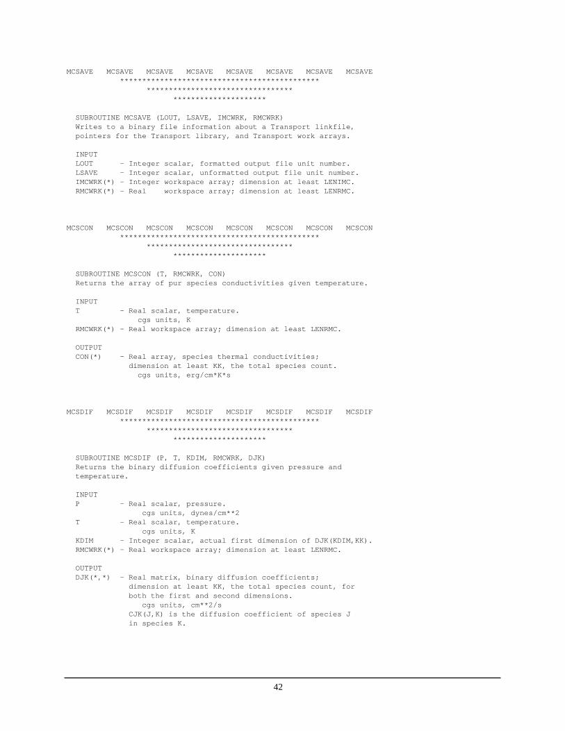
MCSAVE MCSAVE MCSAVE MCSAVE MCSAVE MCSAVE MCSAVE MCSAVE*********************************************

******************************************************

SUBROUTINE MCSAVE (LOUT, LSAVE, IMCWRK, RMCWRK)Writes to a binary file information about a Transport linkfile,pointers for the Transport library, and Transport work arrays.

INPUTLOUT - Integer scalar, formatted output file unit number.LSAVE - Integer scalar, unformatted output file unit number.IMCWRK(*) - Integer workspace array; dimension at least LENIMC.RMCWRK(*) - Real workspace array; dimension at least LENRMC.

MCSCON MCSCON MCSCON MCSCON MCSCON MCSCON MCSCON MCSCON*********************************************

******************************************************

SUBROUTINE MCSCON (T, RMCWRK, CON)Returns the array of pur species conductivities given temperature.


cgs units, KRMCWRK(*) - Real workspace array; dimension at least LENRMC.

OUTPUTCON(*) - Real array, species thermal conductivities;

dimension at least KK, the total species count.cgs units, erg/cm*K*s

MCSDIF MCSDIF MCSDIF MCSDIF MCSDIF MCSDIF MCSDIF MCSDIF*********************************************

******************************************************

SUBROUTINE MCSDIF (P, T, KDIM, RMCWRK, DJK)Returns the binary diffusion coefficients given pressure andtemperature.



cgs units, KKDIM - Integer scalar, actual first dimension of DJK(KDIM,KK).RMCWRK(*) - Real workspace array; dimension at least LENRMC.

OUTPUTDJK(*,*) - Real matrix, binary diffusion coefficients;

dimension at least KK, the total species count, forboth the first and second dimensions.

cgs units, cm**2/sCJK(J,K) is the diffusion coefficient of species Jin species K.

43

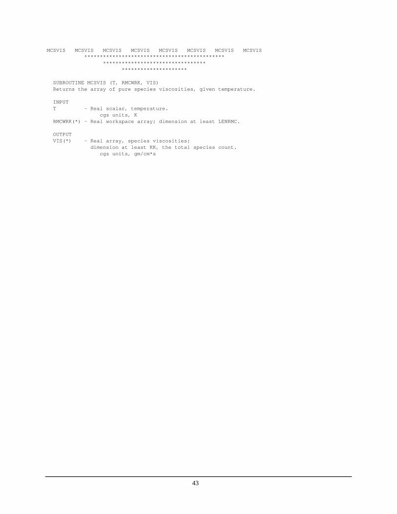
MCSVIS MCSVIS MCSVIS MCSVIS MCSVIS MCSVIS MCSVIS MCSVIS*********************************************

******************************************************

SUBROUTINE MCSVIS (T, RMCWRK, VIS)Returns the array of pure species viscosities, given temperature.


cgs units, KRMCWRK(*) - Real workspace array; dimension at least LENRMC.

OUTPUTVIS(*) - Real array, species viscosities;

dimension at least KK, the total species count.cgs units, gm/cm*s

44

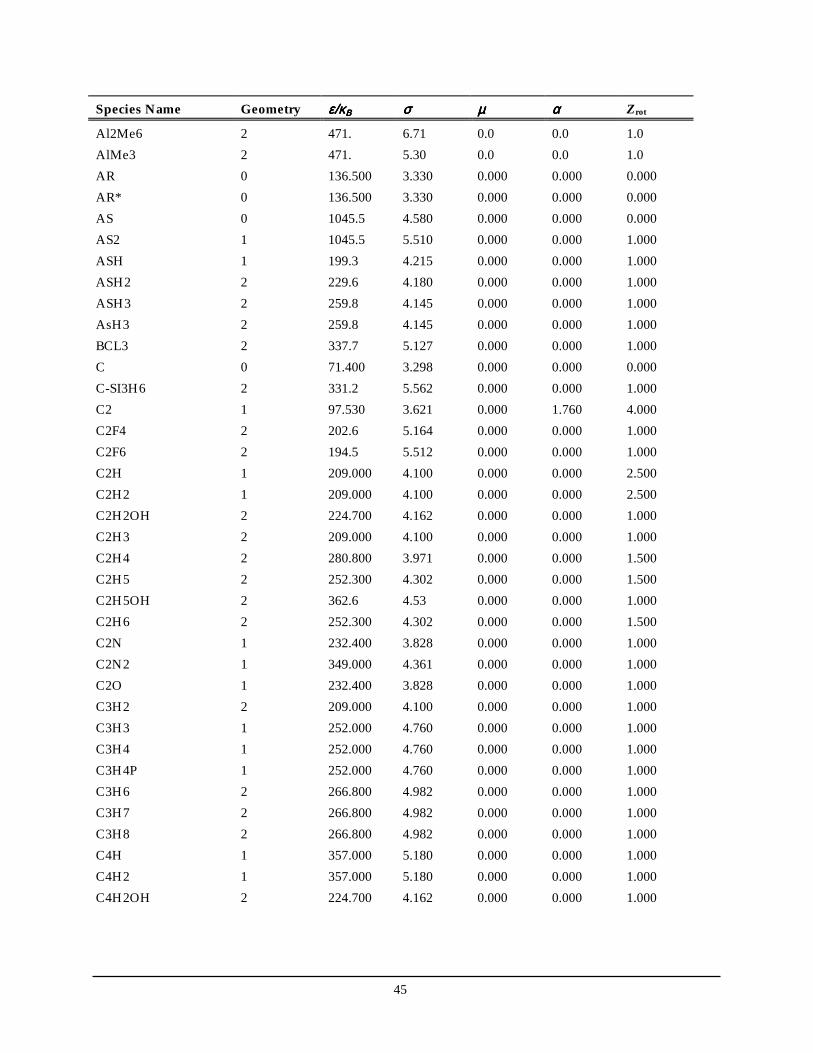
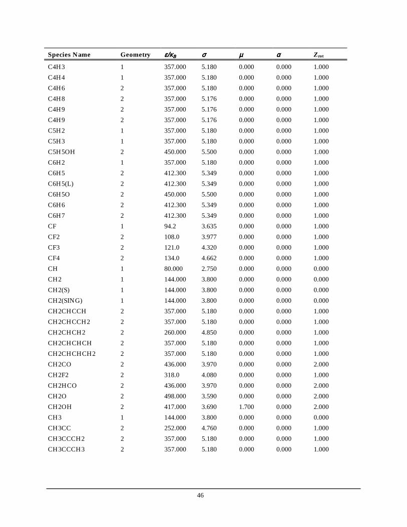
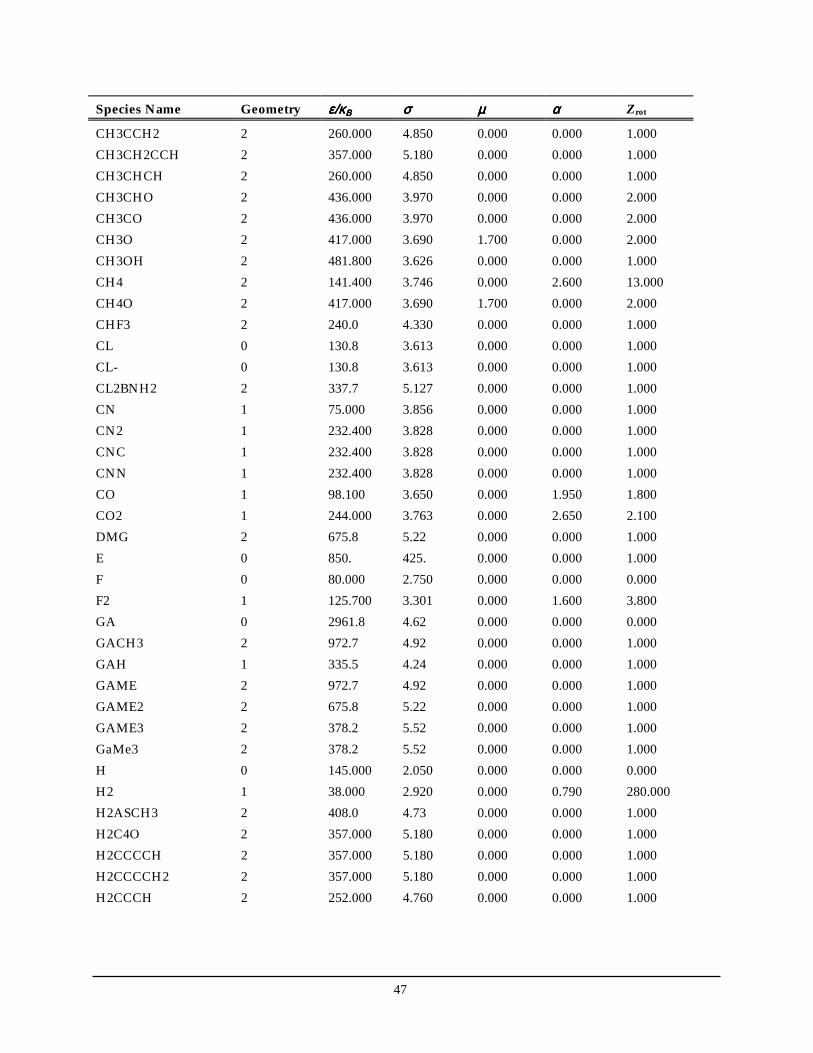
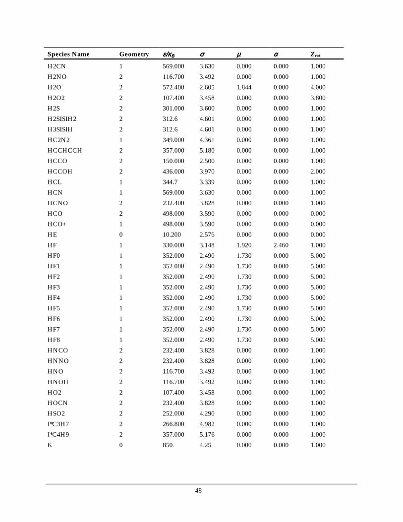
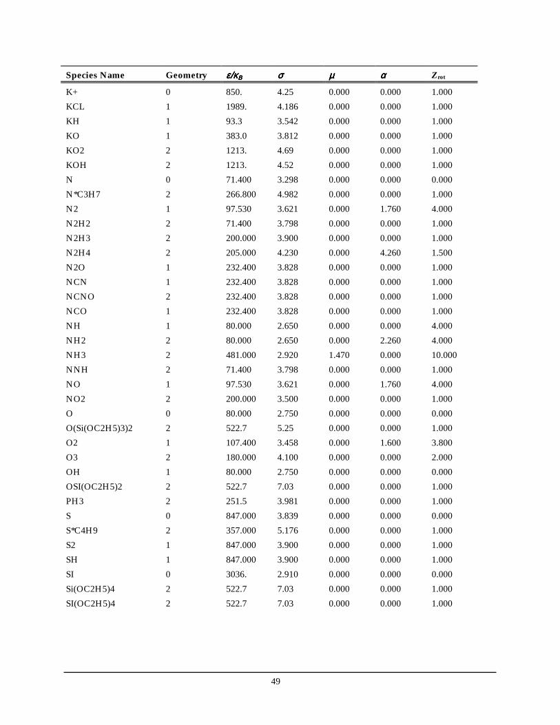
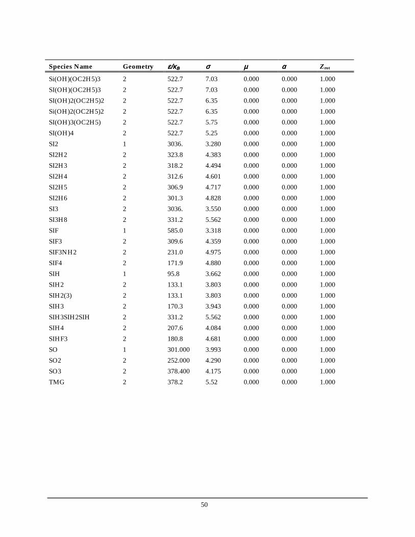
6.6.6.6. TRANSPORT DATABASETRANSPORT DATABASETRANSPORT DATABASETRANSPORT DATABASE In this section we list the database file that is currently included with the TRANSPORT software. While this database file is more of a historical record, we expect that users will want to add their own collection of data to suit their own needs. The database file included with CHEMKIN should not be viewed as the last word in transport properties. Instead, it is a good starting point from which a user will provide the best available data for his particular application. User data of the same format as the database file can now be provided in a supplemental input data file. We recommend using this approach, rather than editing the TRANSPORT database file, since the database file may be updated with subsequent versions of the CHEMKIN Collection. When adding a new species to either the database file or to a supplemental transport data input file, be sure that the species name is exactly the same as it is in the CHEMKIN Thermodynamic Database. Some of the numbers in the database have been determined by computing “best fits” to experimental measurements of some transport property (e.g. viscosity). In other cases the Lennard-Jones parameters have been estimated following the methods outlined in Svehla. 20 The first 16 columns in each line of the database are reserved for the species name. (Presently CHEMKIN is programmed to allow no more than 16-character names.) Columns 17 through 80 are free-format, and they contain the molecular parameters for each species. They are, in order:

1. An index indicating whether the molecule has a monatomic, linear or nonlinear geometrical configuration. If the index is 0, the molecule is a single atom. If the index is 1 the molecule is linear, and if it is 2, the molecule is nonlinear.

2. The Lennard-Jones potential well depthε kB in Kelvins.

3. The Lennard-Jones collision diameter σ in Angstroms.

4. The dipole moment µ in Debye. Note: a Debye is 10-18cm3/2erg1/2.

5. The polarizability α in cubic Angstroms.

6. The rotational relaxation collision number Zrot at 298K.

7. After the last number, a comment field can be enclosed in parenthesis.

45

Species Name Geometry ε/κε/κε/κε/κΒΒΒΒ σσσσ µµµµ αααα Zrot

Al2Me6 2 471. 6.71 0.0 0.0 1.0 AlMe3 2 471. 5.30 0.0 0.0 1.0 AR 0 136.500 3.330 0.000 0.000 0.000 AR* 0 136.500 3.330 0.000 0.000 0.000 AS 0 1045.5 4.580 0.000 0.000 0.000 AS2 1 1045.5 5.510 0.000 0.000 1.000 ASH 1 199.3 4.215 0.000 0.000 1.000 ASH2 2 229.6 4.180 0.000 0.000 1.000 ASH3 2 259.8 4.145 0.000 0.000 1.000 AsH3 2 259.8 4.145 0.000 0.000 1.000 BCL3 2 337.7 5.127 0.000 0.000 1.000 C 0 71.400 3.298 0.000 0.000 0.000 C-SI3H6 2 331.2 5.562 0.000 0.000 1.000 C2 1 97.530 3.621 0.000 1.760 4.000 C2F4 2 202.6 5.164 0.000 0.000 1.000 C2F6 2 194.5 5.512 0.000 0.000 1.000 C2H 1 209.000 4.100 0.000 0.000 2.500 C2H2 1 209.000 4.100 0.000 0.000 2.500 C2H2OH 2 224.700 4.162 0.000 0.000 1.000 C2H3 2 209.000 4.100 0.000 0.000 1.000 C2H4 2 280.800 3.971 0.000 0.000 1.500 C2H5 2 252.300 4.302 0.000 0.000 1.500 C2H5OH 2 362.6 4.53 0.000 0.000 1.000 C2H6 2 252.300 4.302 0.000 0.000 1.500 C2N 1 232.400 3.828 0.000 0.000 1.000 C2N2 1 349.000 4.361 0.000 0.000 1.000 C2O 1 232.400 3.828 0.000 0.000 1.000 C3H2 2 209.000 4.100 0.000 0.000 1.000 C3H3 1 252.000 4.760 0.000 0.000 1.000 C3H4 1 252.000 4.760 0.000 0.000 1.000 C3H4P 1 252.000 4.760 0.000 0.000 1.000 C3H6 2 266.800 4.982 0.000 0.000 1.000 C3H7 2 266.800 4.982 0.000 0.000 1.000 C3H8 2 266.800 4.982 0.000 0.000 1.000 C4H 1 357.000 5.180 0.000 0.000 1.000 C4H2 1 357.000 5.180 0.000 0.000 1.000 C4H2OH 2 224.700 4.162 0.000 0.000 1.000

46


C4H3 1 357.000 5.180 0.000 0.000 1.000 C4H4 1 357.000 5.180 0.000 0.000 1.000 C4H6 2 357.000 5.180 0.000 0.000 1.000 C4H8 2 357.000 5.176 0.000 0.000 1.000 C4H9 2 357.000 5.176 0.000 0.000 1.000 C4H9 2 357.000 5.176 0.000 0.000 1.000 C5H2 1 357.000 5.180 0.000 0.000 1.000 C5H3 1 357.000 5.180 0.000 0.000 1.000 C5H5OH 2 450.000 5.500 0.000 0.000 1.000 C6H2 1 357.000 5.180 0.000 0.000 1.000 C6H5 2 412.300 5.349 0.000 0.000 1.000 C6H5(L) 2 412.300 5.349 0.000 0.000 1.000 C6H5O 2 450.000 5.500 0.000 0.000 1.000 C6H6 2 412.300 5.349 0.000 0.000 1.000 C6H7 2 412.300 5.349 0.000 0.000 1.000 CF 1 94.2 3.635 0.000 0.000 1.000 CF2 2 108.0 3.977 0.000 0.000 1.000 CF3 2 121.0 4.320 0.000 0.000 1.000 CF4 2 134.0 4.662 0.000 0.000 1.000 CH 1 80.000 2.750 0.000 0.000 0.000 CH2 1 144.000 3.800 0.000 0.000 0.000 CH2(S) 1 144.000 3.800 0.000 0.000 0.000 CH2(SING) 1 144.000 3.800 0.000 0.000 0.000 CH2CHCCH 2 357.000 5.180 0.000 0.000 1.000 CH2CHCCH2 2 357.000 5.180 0.000 0.000 1.000 CH2CHCH2 2 260.000 4.850 0.000 0.000 1.000 CH2CHCHCH 2 357.000 5.180 0.000 0.000 1.000 CH2CHCHCH2 2 357.000 5.180 0.000 0.000 1.000 CH2CO 2 436.000 3.970 0.000 0.000 2.000 CH2F2 2 318.0 4.080 0.000 0.000 1.000 CH2HCO 2 436.000 3.970 0.000 0.000 2.000 CH2O 2 498.000 3.590 0.000 0.000 2.000 CH2OH 2 417.000 3.690 1.700 0.000 2.000 CH3 1 144.000 3.800 0.000 0.000 0.000 CH3CC 2 252.000 4.760 0.000 0.000 1.000 CH3CCCH2 2 357.000 5.180 0.000 0.000 1.000 CH3CCCH3 2 357.000 5.180 0.000 0.000 1.000

47


CH3CCH2 2 260.000 4.850 0.000 0.000 1.000 CH3CH2CCH 2 357.000 5.180 0.000 0.000 1.000 CH3CHCH 2 260.000 4.850 0.000 0.000 1.000 CH3CHO 2 436.000 3.970 0.000 0.000 2.000 CH3CO 2 436.000 3.970 0.000 0.000 2.000 CH3O 2 417.000 3.690 1.700 0.000 2.000 CH3OH 2 481.800 3.626 0.000 0.000 1.000 CH4 2 141.400 3.746 0.000 2.600 13.000 CH4O 2 417.000 3.690 1.700 0.000 2.000 CHF3 2 240.0 4.330 0.000 0.000 1.000 CL 0 130.8 3.613 0.000 0.000 1.000 CL- 0 130.8 3.613 0.000 0.000 1.000 CL2BNH2 2 337.7 5.127 0.000 0.000 1.000 CN 1 75.000 3.856 0.000 0.000 1.000 CN2 1 232.400 3.828 0.000 0.000 1.000 CNC 1 232.400 3.828 0.000 0.000 1.000 CNN 1 232.400 3.828 0.000 0.000 1.000 CO 1 98.100 3.650 0.000 1.950 1.800 CO2 1 244.000 3.763 0.000 2.650 2.100 DMG 2 675.8 5.22 0.000 0.000 1.000 E 0 850. 425. 0.000 0.000 1.000 F 0 80.000 2.750 0.000 0.000 0.000 F2 1 125.700 3.301 0.000 1.600 3.800 GA 0 2961.8 4.62 0.000 0.000 0.000 GACH3 2 972.7 4.92 0.000 0.000 1.000 GAH 1 335.5 4.24 0.000 0.000 1.000 GAME 2 972.7 4.92 0.000 0.000 1.000 GAME2 2 675.8 5.22 0.000 0.000 1.000 GAME3 2 378.2 5.52 0.000 0.000 1.000 GaMe3 2 378.2 5.52 0.000 0.000 1.000 H 0 145.000 2.050 0.000 0.000 0.000 H2 1 38.000 2.920 0.000 0.790 280.000 H2ASCH3 2 408.0 4.73 0.000 0.000 1.000 H2C4O 2 357.000 5.180 0.000 0.000 1.000 H2CCCCH 2 357.000 5.180 0.000 0.000 1.000 H2CCCCH2 2 357.000 5.180 0.000 0.000 1.000 H2CCCH 2 252.000 4.760 0.000 0.000 1.000

48


H2CN 1 569.000 3.630 0.000 0.000 1.000 H2NO 2 116.700 3.492 0.000 0.000 1.000 H2O 2 572.400 2.605 1.844 0.000 4.000 H2O2 2 107.400 3.458 0.000 0.000 3.800 H2S 2 301.000 3.600 0.000 0.000 1.000 H2SISIH2 2 312.6 4.601 0.000 0.000 1.000 H3SISIH 2 312.6 4.601 0.000 0.000 1.000 HC2N2 1 349.000 4.361 0.000 0.000 1.000 HCCHCCH 2 357.000 5.180 0.000 0.000 1.000 HCCO 2 150.000 2.500 0.000 0.000 1.000 HCCOH 2 436.000 3.970 0.000 0.000 2.000 HCL 1 344.7 3.339 0.000 0.000 1.000 HCN 1 569.000 3.630 0.000 0.000 1.000 HCNO 2 232.400 3.828 0.000 0.000 1.000 HCO 2 498.000 3.590 0.000 0.000 0.000 HCO+ 1 498.000 3.590 0.000 0.000 0.000 HE 0 10.200 2.576 0.000 0.000 0.000 HF 1 330.000 3.148 1.920 2.460 1.000 HF0 1 352.000 2.490 1.730 0.000 5.000 HF1 1 352.000 2.490 1.730 0.000 5.000 HF2 1 352.000 2.490 1.730 0.000 5.000 HF3 1 352.000 2.490 1.730 0.000 5.000 HF4 1 352.000 2.490 1.730 0.000 5.000 HF5 1 352.000 2.490 1.730 0.000 5.000 HF6 1 352.000 2.490 1.730 0.000 5.000 HF7 1 352.000 2.490 1.730 0.000 5.000 HF8 1 352.000 2.490 1.730 0.000 5.000 HNCO 2 232.400 3.828 0.000 0.000 1.000 HNNO 2 232.400 3.828 0.000 0.000 1.000 HNO 2 116.700 3.492 0.000 0.000 1.000 HNOH 2 116.700 3.492 0.000 0.000 1.000 HO2 2 107.400 3.458 0.000 0.000 1.000 HOCN 2 232.400 3.828 0.000 0.000 1.000 HSO2 2 252.000 4.290 0.000 0.000 1.000 I*C3H7 2 266.800 4.982 0.000 0.000 1.000 I*C4H9 2 357.000 5.176 0.000 0.000 1.000 K 0 850. 4.25 0.000 0.000 1.000

49


K+ 0 850. 4.25 0.000 0.000 1.000 KCL 1 1989. 4.186 0.000 0.000 1.000 KH 1 93.3 3.542 0.000 0.000 1.000 KO 1 383.0 3.812 0.000 0.000 1.000 KO2 2 1213. 4.69 0.000 0.000 1.000 KOH 2 1213. 4.52 0.000 0.000 1.000 N 0 71.400 3.298 0.000 0.000 0.000 N*C3H7 2 266.800 4.982 0.000 0.000 1.000 N2 1 97.530 3.621 0.000 1.760 4.000 N2H2 2 71.400 3.798 0.000 0.000 1.000 N2H3 2 200.000 3.900 0.000 0.000 1.000 N2H4 2 205.000 4.230 0.000 4.260 1.500 N2O 1 232.400 3.828 0.000 0.000 1.000 NCN 1 232.400 3.828 0.000 0.000 1.000 NCNO 2 232.400 3.828 0.000 0.000 1.000 NCO 1 232.400 3.828 0.000 0.000 1.000 NH 1 80.000 2.650 0.000 0.000 4.000 NH2 2 80.000 2.650 0.000 2.260 4.000 NH3 2 481.000 2.920 1.470 0.000 10.000 NNH 2 71.400 3.798 0.000 0.000 1.000 NO 1 97.530 3.621 0.000 1.760 4.000 NO2 2 200.000 3.500 0.000 0.000 1.000 O 0 80.000 2.750 0.000 0.000 0.000 O(Si(OC2H5)3)2 2 522.7 5.25 0.000 0.000 1.000 O2 1 107.400 3.458 0.000 1.600 3.800 O3 2 180.000 4.100 0.000 0.000 2.000 OH 1 80.000 2.750 0.000 0.000 0.000 OSI(OC2H5)2 2 522.7 7.03 0.000 0.000 1.000 PH3 2 251.5 3.981 0.000 0.000 1.000 S 0 847.000 3.839 0.000 0.000 0.000 S*C4H9 2 357.000 5.176 0.000 0.000 1.000 S2 1 847.000 3.900 0.000 0.000 1.000 SH 1 847.000 3.900 0.000 0.000 1.000 SI 0 3036. 2.910 0.000 0.000 0.000 Si(OC2H5)4 2 522.7 7.03 0.000 0.000 1.000 SI(OC2H5)4 2 522.7 7.03 0.000 0.000 1.000

50


Si(OH)(OC2H5)3 2 522.7 7.03 0.000 0.000 1.000 SI(OH)(OC2H5)3 2 522.7 7.03 0.000 0.000 1.000 SI(OH)2(OC2H5)2 2 522.7 6.35 0.000 0.000 1.000 Si(OH)2(OC2H5)2 2 522.7 6.35 0.000 0.000 1.000 SI(OH)3(OC2H5) 2 522.7 5.75 0.000 0.000 1.000 SI(OH)4 2 522.7 5.25 0.000 0.000 1.000 SI2 1 3036. 3.280 0.000 0.000 1.000 SI2H2 2 323.8 4.383 0.000 0.000 1.000 SI2H3 2 318.2 4.494 0.000 0.000 1.000 SI2H4 2 312.6 4.601 0.000 0.000 1.000 SI2H5 2 306.9 4.717 0.000 0.000 1.000 SI2H6 2 301.3 4.828 0.000 0.000 1.000 SI3 2 3036. 3.550 0.000 0.000 1.000 SI3H8 2 331.2 5.562 0.000 0.000 1.000 SIF 1 585.0 3.318 0.000 0.000 1.000 SIF3 2 309.6 4.359 0.000 0.000 1.000 SIF3NH2 2 231.0 4.975 0.000 0.000 1.000 SIF4 2 171.9 4.880 0.000 0.000 1.000 SIH 1 95.8 3.662 0.000 0.000 1.000 SIH2 2 133.1 3.803 0.000 0.000 1.000 SIH2(3) 2 133.1 3.803 0.000 0.000 1.000 SIH3 2 170.3 3.943 0.000 0.000 1.000 SIH3SIH2SIH 2 331.2 5.562 0.000 0.000 1.000 SIH4 2 207.6 4.084 0.000 0.000 1.000 SIHF3 2 180.8 4.681 0.000 0.000 1.000 SO 1 301.000 3.993 0.000 0.000 1.000 SO2 2 252.000 4.290 0.000 0.000 1.000 SO3 2 378.400 4.175 0.000 0.000 1.000 TMG 2 378.2 5.52 0.000 0.000 1.000

51

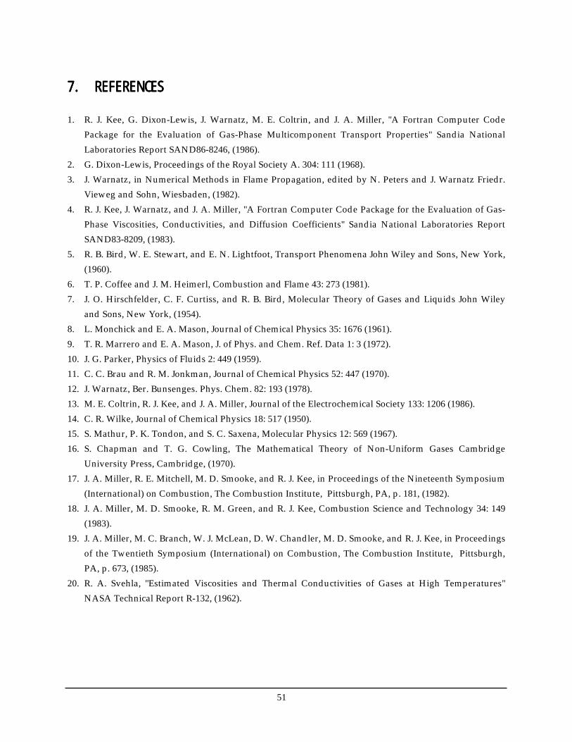
7.7.7.7. REFERENCESREFERENCESREFERENCESREFERENCES 1. R. J. Kee, G. Dixon-Lewis, J. Warnatz, M. E. Coltrin, and J. A. Miller, "A Fortran Computer Code

Package for the Evaluation of Gas-Phase Multicomponent Transport Properties" Sandia National Laboratories Report SAND86-8246, (1986).

2. G. Dixon-Lewis, Proceedings of the Royal Society A. 304: 111 (1968). 3. J. Warnatz, in Numerical Methods in Flame Propagation, edited by N. Peters and J. Warnatz Friedr.

Vieweg and Sohn, Wiesbaden, (1982). 4. R. J. Kee, J. Warnatz, and J. A. Miller, "A Fortran Computer Code Package for the Evaluation of Gas-

Phase Viscosities, Conductivities, and Diffusion Coefficients" Sandia National Laboratories Report SAND83-8209, (1983).

5. R. B. Bird, W. E. Stewart, and E. N. Lightfoot, Transport Phenomena John Wiley and Sons, New York, (1960).

6. T. P. Coffee and J. M. Heimerl, Combustion and Flame 43: 273 (1981). 7. J. O. Hirschfelder, C. F. Curtiss, and R. B. Bird, Molecular Theory of Gases and Liquids John Wiley

and Sons, New York, (1954). 8. L. Monchick and E. A. Mason, Journal of Chemical Physics 35: 1676 (1961). 9. T. R. Marrero and E. A. Mason, J. of Phys. and Chem. Ref. Data 1: 3 (1972). 10. J. G. Parker, Physics of Fluids 2: 449 (1959). 11. C. C. Brau and R. M. Jonkman, Journal of Chemical Physics 52: 447 (1970). 12. J. Warnatz, Ber. Bunsenges. Phys. Chem. 82: 193 (1978). 13. M. E. Coltrin, R. J. Kee, and J. A. Miller, Journal of the Electrochemical Society 133: 1206 (1986). 14. C. R. Wilke, Journal of Chemical Physics 18: 517 (1950). 15. S. Mathur, P. K. Tondon, and S. C. Saxena, Molecular Physics 12: 569 (1967). 16. S. Chapman and T. G. Cowling, The Mathematical Theory of Non-Uniform Gases Cambridge

University Press, Cambridge, (1970). 17. J. A. Miller, R. E. Mitchell, M. D. Smooke, and R. J. Kee, in Proceedings of the Nineteenth Symposium

(International) on Combustion, The Combustion Institute, Pittsburgh, PA, p. 181, (1982). 18. J. A. Miller, M. D. Smooke, R. M. Green, and R. J. Kee, Combustion Science and Technology 34: 149

(1983). 19. J. A. Miller, M. C. Branch, W. J. McLean, D. W. Chandler, M. D. Smooke, and R. J. Kee, in Proceedings

of the Twentieth Symposium (International) on Combustion, The Combustion Institute, Pittsburgh, PA, p. 673, (1985).

20. R. A. Svehla, "Estimated Viscosities and Thermal Conductivities of Gases at High Temperatures" NASA Technical Report R-132, (1962).

Documents

A SOFTWARE PACKAGE FOR THE EVALUATION OF …powers/ame.60636/transport.pdf · GAS-PHASE, MULTICOMPONENT TRANSPORT PROPERTIES ... INTRODUCTION ... Dkj Binary diffusion coefficient