A SOFTWARE IMPLEMENTATION PROGRESS MODEL

by

DWAYNE TOWELL

A THESIS

IN

SOFTWARE ENGINEERING

Submitted to the Graduate Faculty of Texas Tech University in

Partial Fulfillment of the Requirements for

the Degree of

MASTER OF SCIENCE

IN

SOFTWARE ENGINEERING

Approved

Chairperson of the Committee

~^

Accepted

Dean of the Graduate School

August, 2004

ACKNOWLEDGEMENTS

I would like to thank my wife, Lydia, for her support and understanding. I

could not have done this work without her support.

I would also like to thank my advisor, Dr. Jason Denton, for his guidance and

critical review. His understanding of and advice about the academic world was an

invaluable aid during my transition and this work.

Many thanks go Terry Hamm and Roger Arce for access to project archives

that made this study possible. Without their support this would still only be an idea.

Additional thanks go to friends and family who supported this work by many

different contributions. They include Roger Bonzer, Dr. Mike Frazier, Dr. Rusty

Towell, Marta E. Calderon-Campos, and countless others. Thank you all.

This work is dedicated to Ayrea and Robert, my children and the world's

greatest kids, hands down.

TABLE OF CONTENTS

ACKNOWLEDGMENTS ii

LIST OF TABLES vii

LIST OF FIGURES viii

I. INTRODUCTION 1

1.1 Need for Models 3

1.2 Model Requirements 4

1.3 Implementation Progress Model Requirements 6

II. RELATED WORK 9

2.1 Implementation Evaluation and Control 10

2.2 Time-Series Shape Metrics 13

2.3 Process Models 15

m . RESEARCH DESIGN 18

3.1 Existing Progress Models 18

iii

3.2 Implementation Progress Model 21

3.3 Model Interpretive Value 25

3.4 Data Requirements 28

3.5 Data Collection 31

3.6 Data Source 32

IV. EFFORT METRICS 34

4.1 Source Lines of Code 34

4.2 McCabe Complexity 36

4.3 Halstead Volume 38

4.4 Other Metrics 40

V RESULTS 42

5.1 Alternative Models 42

5.2 Model Fitting Results 44

5.3 Anomalous Data Sets 49

5.4 Model Applicability 51

iv

5.5 Conforming Cases 61

M. CONCLUSIONS 67

6.1 Limitations 67

6.2 Interpretation 68

6.3 Future Work 69

REFERENCES 71

ABSTRACT

Current software project management techniques rely on collecting metrics

to provide the progress feedback necessary to allow control of the project; however,

interpretation of this data is diflScult. A software implementation progress model is

needed to help interpret the collected data. Criteria for an implementation progress

model are developed and an implementation progress model is proposed. Findings

from the studied projects suggest the model is consistent with the observed behav­

ior. In addition to quantitative validity, the model is shown to provide meaningful

interpretation of collected metric data.

VI

LIST OF TABLES

5.1 Average squared residual error (/?^) for implementation progress models measuring source lines of code changed (SLOCC) by project. 53

5.2 Average squared residual error (R^) for implementation progress models measuring code churn (CHURN) by project. 54

5.3 Average squared residual error (7? ) for implementation progress models measuring cyclomatic complexity change (MCC) by project. 55

5.4 Average squared residual error (W^) for implementation progress models measuring Halstead length change (HLC) by project. 56

5.5 Source lines of code change (SLOCC) progress model parameters and R^ relative to linear R^. 62

5.6 Code churn (CHURN) progress model parameters and R^ relative to linear R^. 63

5.7 Cyclomatic complexity change (MCC) progress model parameters and i?2 relative to linear R^ 64

5.8 Halstead length change (HLC) progress model parameters and R^ rel­ative to linear R^. 65

Vll

LIST OF FIGURES

3.1 Accumulated change metrics for a typical project by day. 19

3.2 Idealized implementation velocity as a function of time. 23

3.3 Idealized implementation progress as a function of time. 23

5.1 Progress measured via accumulated Halstead length change (HLC) for project nine and progress model curves (with R^). 45

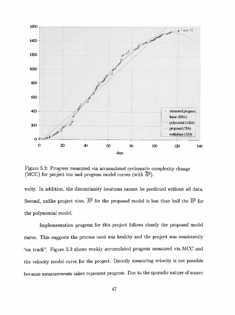
5.2 Progress measured via accumulated cyclomatic complexity change (MCC) for project ten and progress model curves (with R^). 47

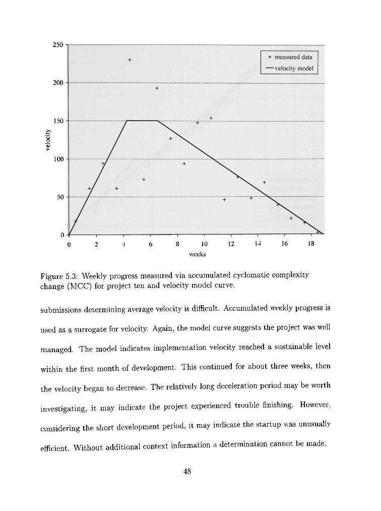
5.3 \\'eekly progress measured via accumulated cyclomatic complexity change (MCC) for project ten and velocity model curve. 48

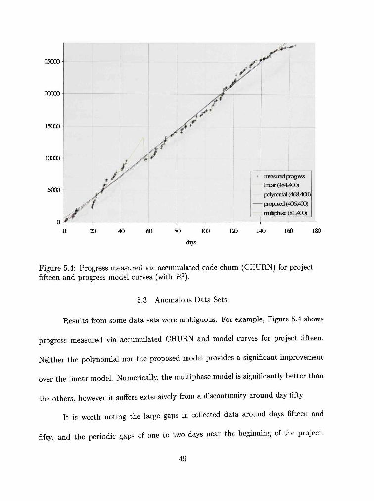
5.4 Progress measured via accumulated code churn (CHURN) for project fifteen and progress model curves (with R^). 49

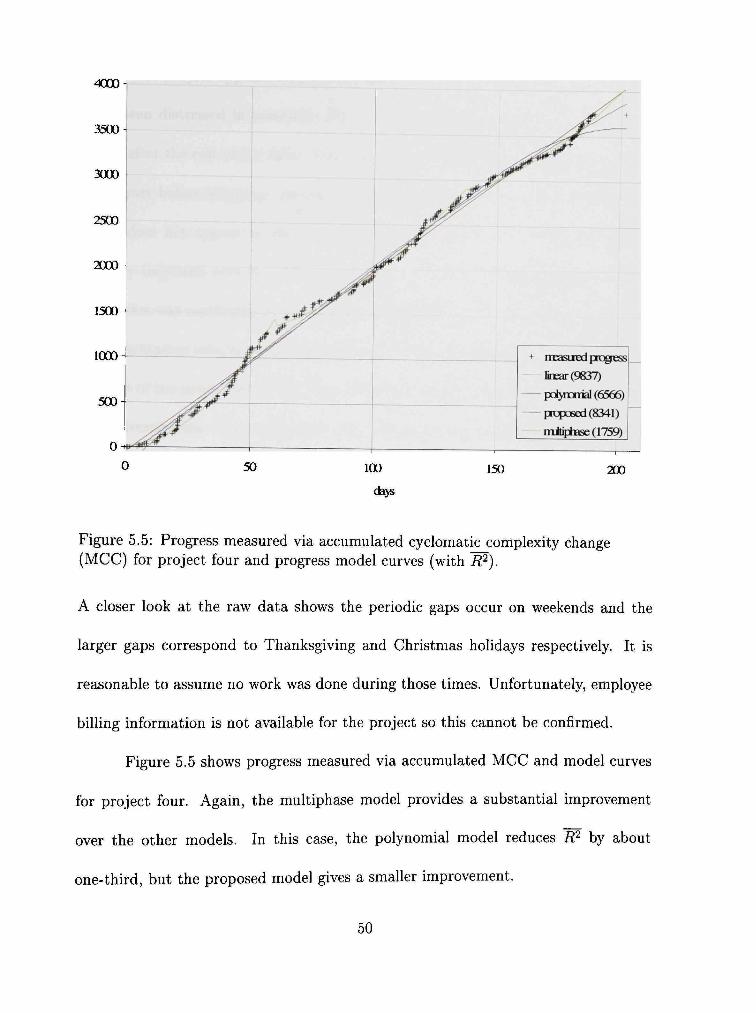
5.5 Progress measured via accumulated cyclomatic complexity change (MCC) for project four and progress model curves (with R^). 50

5.6 Source lines of code change (SLOCC) average squared residual error (R^) relative to linear R^. 57

5.7 Code churn (CHURN) average squared residual error (R^) relative to linear W. 58

5.8 Cyclomatic complexity change (MCC) average squared residual error (i?2) relative to hnear R'^. 59

5.9 Halstead length change (HLC) average squared residual error (i?^) rel­ative to linear i?^. 60

viu

CHAPTER I

INTRODUCTION

Modern software development practices rely on periodically collected software

metric data to provide management with feedback about the project and the process

used to de\elop it. Metric data is most commonly used in the area of quality as­

sessment. Well-defined metrics exist to report on quality attributes such as expected

number of remaining faults. However, other areas, such as implementation progress,

make much less use of metric data for feedback. Metrics, such as total source lines

of code, could be used to report on implementation progress but measures such as

these have not been leveraged as strongly as quality assessment has used its mea­

sures. Metric data is widely regarded as a valuable management feedback tool, yet it

is generally not used to monitor implementation progress.

An implementation progress model is presented and shown to identify project

phase boundaries, express the rate of implementation during each phase, and allow

objective comparisons between projects. This study provides a framework to help

interpret periodically collected implementation data. This work develops a model

for interpreting implementation progress. The proposed progress model uses existing

implementation artifact metrics, matches our intuitive understanding of the imple­

mentation progress, and allows project estimation based on parameter estimates.

Well-defined and proven metrics exist for many areas of software development

including especially quality assessment. Implementation progress has no such estab-

1

lished metrics. Several existing metrics measure size-related attributes. While these

size-related metrics may have been originally developed to support quality assess­

ment, they can be used to monitor progress in terms of size. Project size is important

because it is invariabh' used to estimate the resources needed and assess the project's

status with regard to the schedule (DeMarco 1982; Albrecht and John E. Gaffney

1983; Lind and \'airavan 1989; Jorgensen 1995). This compelling management need

for feedback about implementation progress should demand its use. Its absence may

be because metrics have not been established to support implementation progress

feedback.

The lack of proven implementation progress metrics has been a barrier to any

attempt to monitor implementation progress. However, the lack of a proven metric

is not insurmountable. Size metrics are abundant and deriving a progress metric

from a size metric can be accomplished by taking the difference in consecutive size

measurements. A far larger barrier than the lack of a metric is the lack of a proven

implementation progress model. Periodically collected data is rich in detailed infor­

mation but is not inherently meaningful. A model provides a specific interpretation

of the data and allows meaning to be extracted. An implementation progress model

will allow periodically collected implementation data to be interpreted.

1.1 Need for Models

Models bridge the gap between concrete sampled data and expectations. On

a small scale, models act as predictors to set expectations over the next few data

samples. For example, a defect model may indicate the number of faults to be found in

the next release candidate. The degree to which the actual number of faults discovered

diflfers from the predicted value can be an indication of unexpected circumstances

within the project. For instance, an unusually low value (when compared with the

predicted value) may indicate fewer code changes were made than expected, or that

less testing was performed than expected. Management has been forewarned; an

investigation can be made and the appropriate response can be taken. This small

scale feedback provides valuable and timely feedback to management within the scope

of the project.

In addition to this small scale feedback, models provide feedback on a larger

scale, outside the scope of a single project. Large scale feedback assumes an entire

project can be "boiled down" to its essence. Large scale feedback is less concerned

with local variations and more concerned with the overall picture portrayed by the

data. This "essential" portrait is regularly required by management, with or without a

formal model. Without a formal model members of management must rely on guesses

and antidotal evidence. In contrast to this haphazard approach, a formal model es­

tablishes a rigorous evaluation. A formal model establishes the critical parameters

within the system. Using a formal model, projects may be evaluated or compared in

terms of the model paramc>ters. Model parameters allow evaluation and comparisons

to be based on defendable data rather than guesses and hearsay. Additionally, given

estimated values for the parameters, the model can make predictions about the out­

come. This relationship between parameters (input) and predictions (output) codifies

a causal effect believed to be true within the system.

1.2 Model Requirements

The primary purpose of a model is to provide a documented method of in­

terpreting a set of data. In many cases the interpretation is masked by the sheer

quantity and detail of the data available. Information is revealed when the data is

interpreted in a particular way. The interpretation results can be used to evaluate

past performance, assess the current situation, and make predictions about future

performance. The interpretation can also be used to compare multiple data sets.

Results from the same model, applied to several data sets, allow the data sets to be

easily compared in terms of the model. The model provides a systematic method for

comparing projects.

One type of model interprets series data by attempting to fit collected data

to a family of curves. The single curve which best fits the data is used to describe

the data in terms of the model. The specific values used to generate the best fitting

curve are considered parameters of the model. Parameters of a model reveal one or

more dimensions of the collected data. In this case, parameters can be considered an

4

output of the model. Collected data is the input and results summarizing that data

are produced. Parameters can also be used as input resulting in expected sample data.

When used in this way, models make predictions based on estimated parameters. In

either case, the expected progress as defined by the model is given by the model curve.

The model equation and a specific set of parameters define the model curve.

A valuable model is one that produces a clear and concise interpretation of

the data. Part of this interpretation is in the form of the specific values for the model

parameters. For example, consider two models, one uses only two parameters while

the other has eight parameters. Even though the eight-parameter model may predicts

the data "twice" as well, it may not be the better model if its parameters have no

particular meaning or are hard to estimate.

Models should have as few parameters as possible while still modelling the

data with sufficient accuracy. Fewer parameters means the model is easier to under­

stand. Part of understanding a model is understanding the relationships between the

parameters. Parameters are related by the affects each has on the others. Knowing

the trade-offs between parameters is necessary to understand a model. This is easier

if the model contains fewer parameters.

In addition to relatively few parameters, individual model parameters should

be understandable. Understandable parameters produce simple results with meaning.

On the other hand, meaningless parameters do not help to simplify or interpret the

data since they must again be interpreted. Parameter meaning is even more important

when the model is used as a predictor for new projects. In this case, model parameters

must be estimated before any data has been collected. If the individual parameters

are well understood better estimates for each will be made. Better estimates will

produce better predictions.

Related to individual parameter meaning is the parameter unit. Model pa­

rameters should be expressed in well-known units, rather than new or arbitrary ones.

Parameters with direct interpretations allow the model results to be easily understood

and used. Well-known units are also much easier to estimate. Again, this allows for

better predictions.

Model parameters should be few in number, directly interpretable, and mea­

sured in existing units. These properties give the model parameters the most meaning

and thus give the model the most "clarifying power".

1.3 Implementation Progress Model Requirements

In addition to general model requirements, an implementation progress model

must be compatible with existing models. Implementation progress is not a new con­

cept. An informal progress model already exists; it can be seen in project vocabulary

and assumptions. For example, project members speak of "getting over the learning

curve" and being "up to speed". This informal model is commonly used to answer

common project status queries, such as:

What is the expected completion date based on the current pace? What was the size of the total effort for that project? What fraction of the total effort is currently done? What fraction of the total effort will be done by a certain date?

A proposed implementation model should serve the same purpose as the informal

model. The model must help provide answers to questions about implementation

speed and progress of current and future projects.

The informal progress model captures another key attribute of implementa­

tion progress. The informal model acknowledges that project speed is not constant

throughout a project: projects "ramp up" and "slow down". These phrases refer to

project speed and suggest the ability or desire to determine implementation velocity.

As envisioned by experienced project managers, this velocity increases at the begin­

ning and decreases near the end (McConnell 1998). A formal implementation progress

model should be informed by this experience and capture the canonical variations in

velocity during implementation.

In summary, the desired attributes of a formal implementation progress model

include: relatively few parameters, understandable parameters, well-known parameter

units, consistency with informal progress model, and the ability to answer manage­

ment questions involving size and velocity.

The next chapter (II) discusses supporting work indicating the need for a

progress reference model. Chapter III describes the proposed implementation progress

model, hypothesis, and research process. The specific metrics used are presented in

Chapter IV including description, discussion and support for each. Results from

actual projects are presented in Chapter V. Finally, conclusions and directions for

future study are in Chapter VI.

CHAPTER II

RELATED WORK

Previous work applying software metrics to the development process has pri-

marih' been targeted at tasks before and after implementation. Much work has been

done in the pre-implementation stages to improve effort prediction and estimation (Al­

brecht and John E. Gaffney 1983; Lind and Vairavan 1989; Jorgensen 1995; Boraso,

Montangero, and Sedehi 1996; Turski 2002). Metrics have also been used to evaluate

architectural design before implementation. Significant work has been done in the

post-implementation stages to predict failure rates, both for a product as a whole

as well as for individual modules (Jelinski and Moranda 1971; Goel and Okumoto

1979; van Solingen and Berghout 1999; Fenton and Neil 1999; Schneidewind 1999).

However, substantially less work has been published regarding the use of metrics for

assessment, monitoring, or control of the implementation stage itself.

DeMarco asserts "you can't control what you can't measure" (DeMarco 1982,

page 3). Indeed, every researcher proposing, defending, or merely discussing a metric

agrees the reason behind metrics and measuring is to gain some degree of understand­

ing and control over the complex process of software development (Fenton and Neil

2000). Recent studies have focused attention on how to use the vast array of data

generated by existing measures.

Published works emphasizing how to use the potentially enormous data avail­

able can be coarsely divided into three groups. Many works assert metrics should be

9

used to assist in monitoring, evaluation and control of projects during the implemen­

tation phase (DeMarco 1982; BasiU and Rombach 1988; Boehm 1988; Lott 1993; van

Sohngen and Berghout 1999; Kirsopp 2001). Other researchers recommend specifi­

cally that time-series metrics data be used to monitor and evaluate projects (DeMarco

1982; McConnell 1998; Schneidewind 1999). Finally, several researchers emphasize

the insight gained from causal models over correlative models (Powell 1998; Fen­

ton and Neil 2000; Turski 2002). They suggest models which provide an inherent

causes-relationship are more valuable than simpler correlation models.

2.1 Implementation Evaluation and Control

DeMarco presents a development process relying on steadily improving es­

timates to provide feedback and control during all phases of software development

(DeMarco 1982). Metrics collected at each stage of development provide raw data for

creating an improved estimate for the next stage. Metrics from the current project as

well as previous projects are used to inform decisions. Inherent throughout his work is

the requirement for continuing feedback via improving estimates, allowing the devel­

opment effort to be directed. A compelling case supporting estimate reviews, process

metrics, cost models and quality improvement is developed. DeMarco identifies and

recommends metrics appropriate for each stage of development.

In discussing appropriate metrics for the implementation stage DeMarco al­

ludes to process metrics such as compilation rate but does not explore them. The

10

primary implementation measure is code weight, which is defined as a product of two

dimensions: size and complexity. DeMarco defines code size as information content

within a program. He recommends using Halstead's volume metric (Halstead 1977) to

find size. Several alternatives for measuring complexity are presented, but McCabe's

cyclomatic complexit}' measure (McCabe 1976) is recommended. Using these two

dimensions as parameters, an algorithm is presented for computing implementation

weight. Historical data from similar projects and environments is also used to provide

scaling factors. According to DeMarco, the primary motivation for computing imple­

mentation weight is to improve future project estimates. However, he also calls it a

"project predictor", that is, it should predict the final size of the project accurately.

According to the system presented by DeMarco, the measure should be taken once

near the middle of implementation. The progress model described in this study may

provide a better estimate of implementation size. Since the proposed model considers

the complete project history, not simply a single point in time, it is less susceptible

to anomalies.

Boehm takes a broader approach to development feedback than simply fo­

cusing on improved estimates. He introduces a software development methodology

whose principle goal is risk management (Boehm 1988). His spiral model of software

development relies on risk evaluation as the impetus for each unit of work, whether

the work unit is a prototype, design document, or code. Risk management impUes

the ability to control what is being managed. This agrees with DeMarco's argument

11

that our need to measure the software development process stems from our desire to

control the process (DeMarco 1982). Boehm's methodology assumes feedback metrics

exist to inform the risk evaluation process, but does not dictate specific measures or

measurement processes.

Addressing the selection of appropriate metrics for quality control, Solingen

and Berghout defined the Goal/Question/Metric Method (GQM) of improving soft­

ware quality (van Solingen and Berghout 1999). GQM integrates metrics into the

development process in order to answer questions about quality raised by corporate

goals. Their methodology relies on the ability to follow the connection between cor­

porate goals and specific metrics, in both directions. Measurements are defined by

goals and the results interpreted in terms of those goals. In the area of quality control,

well developed process models exist to help define and interpret metrics. However,

implementation models in general, and implementation progress in particular, have

not been as well developed.

Kirsopp addresses the need to capture development models and enough data

to evaluate them. He strongly argues that the software development process needs

measurements for feedback and that the integration must be close, detailed and ap­

propriate (Kirsopp 2001). Organizations must support metrics outside of a single

project in order to validate the process, validate the results, and collect historic data.

All three of these are required to assist future project estimates. An experience fac­

tory provides a repository for captured experiences and models, allowing reuse within

12

an organization. Kirsopp cites the TAME (Tailoring a Metric Environment) Project

(Basili and Rombach 1988) as a working example of an experience factory.

Lott provides an alternative approach; instead of suggesting or analyzing met­

rics, he studied several available and proposed software engineering environments

(Lott 1993). Many of these environments include integrated tools for collecting nu­

merous metrics about various development artifacts created. Lott suggests collected

data can be used to guide development and to call attention to atypical patterns wor­

thy of investigation. In this regard, he assumes time-series data will be collected and

evaluated. Inherent in this idea is the development of a canonical pattern or typical

shape for a particular metric. Unfortunately, neither Lott nor the systems studied

define how to select or interpret the automatically collected measurements.

2.2 Time-Series Shape Metrics

In addition to estimation, DeMarco briefly notes that process metrics, such as

compilation rate, can be used to identify project dysfunction and impending problems

(DeMarco 1982). Periodic sampling of a metric allows the value measured to be

graphed against time. For some measures, such as compilation rate, "healthy" projects

may all have similar shapes when viewed as time-series data. If this is the case,

"unhealthy" projects can be detected if or when they deviate from the canonical shape.

For example, DeMarco suggests compilation rates that continue at a steady rate

without showing any decline may be an indication of a "thrashing" development team.

13

While this particular evaluation may not apply to all development environments, the

idea of a "healthy" canonical shape can be applied to all environments. In another

instance, he recommends reporting test progress as a graph showing measurements

against time. Time-series graphs make it clear how test progress has been proceeding

and how its trends change over time. In general, comparing the current project

with similar historic projects using graphs can highlight abnormal trends which may

be an indicator of trouble. Given DeMarco's emphasis on continuous monitoring

and improvement, it is surprising he does not suggest using implementation artifact

metrics, such as size or complexity, to monitor implementation progress.

Schneidewind used time-series metrics to create a method for evaluating pro­

cess stability (Schneidewind 1999). He illustrates its use by evaluating the process

stability of the NASA Space Shuttle flight software development efforts. Schnei­

dewind emphasizes that metric trends are a significant indicator of the underlying

process and monitoring the trends can provide feedback about the process. To quan­

tify these trends, he introduces two new classes of indirect metrics. A change metric

is computed using differences in consecutive values of a traditional metric. This met­

ric can be viewed as the derivative of the primary metric. The other class of indirect

metric introduced is the shape metric. A shape metric is derived from the curve of

the time-series metric data when graphed against time. For example, one shape met­

ric suggested is the time at which the failure rate is highest. Lower values for this

metric may indicate process stability, while higher values may indicate instability in

14

the development process. A strong case is presented for the use of time-series data,

and indirect metrics derived from it, in the context of process stability. Monitoring

progress during the development stage using change and shape metrics is an obvious

extension of this study.

McConnell understands typical "code growth" on a project to contain three

distinct phases (McConneU 1998). In the first phase, architectural development and

detailed design generate very little code. The second phase provides staged deliveries

and includes detailed design, coding, and unit testing. During this phase code growth

is very high. During final release, the third phase, code growth slows to a crawl.

McConnell shows a graph depicting a typical code growth pattern for a well-managed

project. He indicates the phase transitions occur at approximately 25% and 85% of

the total development time, but acknowledges that this varies to some degree. His

main point is periodic monitoring of code size is a valuable feedback tool for managers.

No details are given about the specific metric(s) involved or the process used to collect

the data. The proposed progress model clarifies how metrics are used and provides a

specific interpretation of the three phases documented by McConnell.

2.3 Process Models

Powell expands the role of software measurement to explicitly include not

only prediction and control but also assessment and understanding (Powell 1998). He

makes arguments for assessment similar to those presented by Boehm and DeMarco

15

for prediction and control. Regardltiss of the motive, measurements are always based

on assumptions about the process in which the measurement is taken. Powell states

"it is impossible to talk about measurements without implying some form of [process]

model" (Powell 1998, page 5). Before measurements can be taken, and before metrics

can be determined, a model of the development environment must be chosen.

Fenton and Neil proposed using Bayesian belief networks (BBNs) to model

development environments (Fenton and Neil 2000). BBNs integrate causality, uncer­

tainty, and expert subjective input to generate answers and assist in decision making.

They observe the current lack of metrics in common practice, within the software

development community, and blame a lack of realistic decision making models. Many

existing models are simplistic in that they show strong correlations between measures

but do not properly model causality. Using BBNs allows better causality modeUing

to be achieved. This allows the answers generated to be both more accurate and

traceable. BBNs encode beliefs about the causality of a process in the network. The

parameters can be populated with known values, known distributions or even sus­

pected distributions. Answers computed show not only the likely result but its range

and distribution. BBNs provide a general solution to the problem of model encoding.

Turski presents a model for understanding the observed rate of software growth

as a function of time (Turski 2002). Using the number of modules as the dependent

variable and uniform interrelease intervals as the independent variable, he shows size

correlates strongly with the third root of time {size = \/time). While defendable on

16

the bases of Lehman's Laws of Software Evolution (Lehman, Ramil, Wernick, and

Perry 1997), Turski uses a simple mental model to understand the same relationship.

He suggests envisioning a system as a sphere with "surface" modules being easy to

modify while "interior" modules are much harder to modify. With this model in mind,

it is easy to see that the proportion of easy modules to hard modules tends toward

zero as the project (sphere) grows with time.

Turski believes that simple and manageable models, such as that described

above, provide powerful insights into understanding the forces at work in software

development. In particular, models which exhibit causal relationships rather than

simple statistical correlations provide not only better interpretation but improved

understanding of the process. He suggests similar "back-of-an-envelope" models be

developed precisely because they are simple to understand and intuitive. He expresses

concern that so few causal-model-based arguments have been presented in the litera­

ture to date. The progress model proposed here includes such a simple and intuitive

interpretation of the implementation process.

17

CHAPTER III

RESEARCH DESIGN

This chapter presents the implementation progress model studied and proce­

dures used in the study. First, the proposed model is described in detail along with

the rationale for it. This is followed by a description of the analysis process. Then,

the data required for the study is discussed. Finally, a summary of where appropriate

projects were found and how the data was collected is presented.

3.1 Existing Progress Models

Project managers have developed an intuition about what should occur during

a software development effort. An implementation progress model should be consis­

tent with this experience. A condensed version of this collective wisdom is presented

by McConnell (McConneU 1998). He uses code growth as an measure of progress and

provides a nominal code growth pattern as well as a range of normal variations for

well-run projects. An appropriate progress model should reflect the basic shape of

accepted norms such as those presented by McConnell.

Another constraint on choosing an appropriate implementation progress model

is its interpretive power. Interpretation of metric data relies on some understanding of

or belief about the underlying process. For example, changes in the rate of progress

in an otherwise stable environment may indicate the project has transitioned to a

18

70000

days

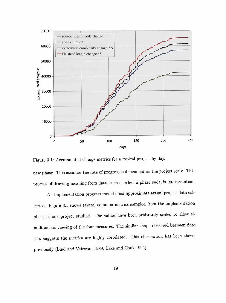
Figure 3.1: Accumulated change metrics for a typical project by day.

new phase. This assumes the rate of progress is dependent on the project state. This

process of drawing meaning from data, such as when a phase ends, is interpretation.

An implementation progress model must approximate actual project data col­

lected. Figure 3.1 shows several common metrics sampled from the implementation

phase of one project studied. The values have been arbitrarily scaled to allow si­

multaneous viewing of the four measures. The similar shape observed between data

sets suggests the metrics are highly correlated. This observation has been shown

previously (Lind and Vairavan 1989; Lake and Cook 1994).

19

The data in Figure 3.1 is very similar to that described by McConnell. Each

data series has approximately the same shape, an S-like curve. Initially the project

makes very little headway, but over a period of about seventy days the rate of progress

improves. During this time the project experiences a period of increasing speed

as resources are added and things get "up to speed". For the next 100 days the

metrics show approximately linear progress. Here the project experiences a time of

continuous, even-paced development during which much of the work is accomplished.

This is the period of highest efficiency for the project. Finally, during the last eighty

days progress continues but at a steadily slowing pace. The project experiences a

time of lower efficiency as it nears completion and attention to detail is paramount.

This graph demonstrates the important characteristics of typical progress data.

Overall progress is not linear with time, but approximately linear progress occurs

during the middle of the project. This sample and experience suggest the beginning

and end of the project contribute the least to overall progress. This means the fastest

pace occurs during the middle of the project while the ends are slower paced. The

slope of the progress curve indicates the speed of progress. The graph is consistent

with both expectations about progress and speed. The slope of progress (velocity)

can be used to determine how and when the project transitioned from "ramping up"

to its sustainable rate of progress. Likewise, near the end of the project, a slope

change indicates a change in velocity which may indicate a change in process and

possibly goals.

20

The typical "slow" startup phase may be partly due to resources being added,

team members establishing relationships, and processes developing within the project

group. McConnell suggests detailed requirements understanding and architecture

may still be under development during the startup phase as well (McConnell 1998).

Steady "fast" development begins only after this initial investment period. As the

project nears completion the rate of progress decreases. This slowing may be due to

inefficiencies related to critical paths, loss of resources, defect removal and attention

to detail required to meet flnal deliveries.

DeMarco acknowledges this non-linear relationship in his advice about when

to collect implementation metrics (DeMarco 1982). He strongly advocates the need

for feedback throughout the development process, however recommends only a single

sampling of size metrics near the middle of the implementation phase. This incon­

sistency is understandable after examining his assumptions. DeMarco uses a linear

model which is required to pass through the origin and the current project implemen­

tation weight (size). It can be easily seen in Figure 3.1 the only time an origin-based,

linear model will be accurate is if the sample point is near the middle of the project.

3.2 Implementation Progress Model

Before attempting to characterize implementation progress for a complete

project, it is appropriate to consider a definition for implementation progress. Soft­

ware implementation is the activity of creating artifacts which contribute to the goal

21

of delivering a working system. Implementation progress is the amount of change in

an artifact over the time needed to produce the change. Progress is best measured as

the sum of many changes rather than any single measure. This is due to the volatile

nature of implementation; code may be added, removed, moved or changed. The sum

of these individual measurements is a better approximation of the total progress than

any single measurement. This is similar to the way an odometer is a better measure

of distance travelled than simply the distance from the starting point.

An individual implementation progress measurement captures implementation

artifact change over time. Change over time is velocity, so individual progress mea­

surements attempt to capture implementation velocity. If implementation velocity

is in anyway analogous to velocity found in the natural world, it cannot change in­

stantaneously. It is reasonable to assume implementation velocity does not change

instantly, so the first derivative (velocity) of the implementation progress model must

be continuous.

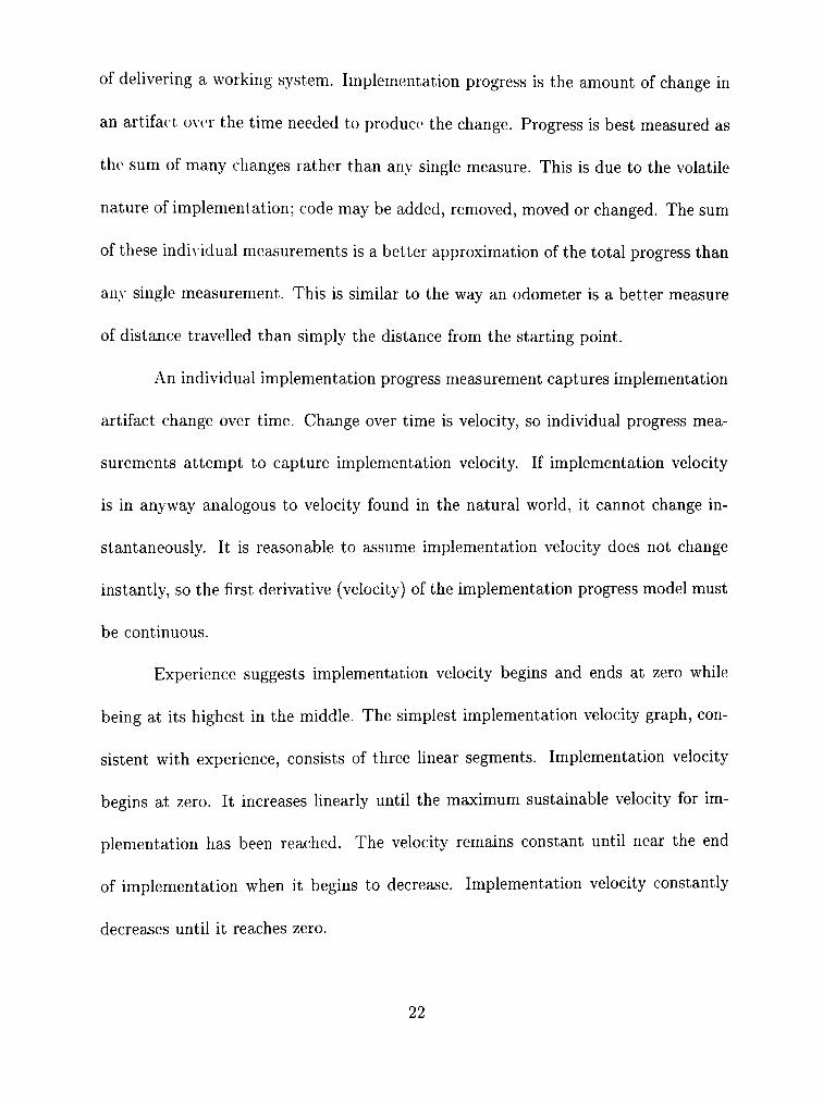
Experience suggests implementation velocity begins and ends at zero while

being at its highest in the middle. The simplest implementation velocity graph, con­

sistent with experience, consists of three linear segments. Implementation velocity

begins at zero. It increases linearly until the maximum sustainable velocity for im­

plementation has been reached. The velocity remains constant until near the end

of implementation when it begins to decrease. Implementation velocity constantly

decreases until it reaches zero.

22

project time

Figure 3.2: Idealized implementation velocity as a function of time.

jrog

res

project time

Figure 3.3: Idealized implementation progress as a function of time.

Figure 3.2 shows the idealized implementation velocity for a project as a func­

tion of time. The horizontal, center phase represents the steady, efficient development

observed in the middle of the implementation phase. The positive slope at the left

represents increasing velocity as implementation "gathers speed". This increasing pace

may be the result of adding resources or team members establishing roles within the

project. The negative slope at the end of the graph shows the implementation phase

decreasing speed as the end approaches. The slowing may be due to inefficiencies

related to critical paths, loss of resources, and attention to detail required to meet

final deliveries. Slope changes in a graph showing velocity are good indicators of a

change in the environment, such as mode of development or goal for the project. In

the idealized graph shown in Figure 3.2 the slope changes indicate respectively that,

the project has reached its maximum sustainable velocity, and the team is attempting

to complete all tasks rather than maintain velocity.

23

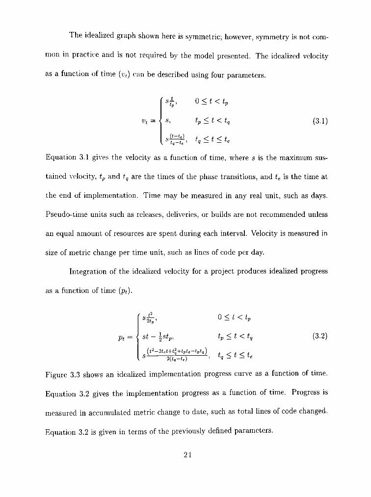
The idealized graph shown here is symmetric; however, symmetry is not com­

mon in practice and is not required by the model presented. The idealized velocity

as a function of time (vt) can be described using four parameters.

vt = <

sj-, 0 <t <tp

s, i"P j^ 6 ^s, LQ (3.1)

Equation 3.1 gives the velocity as a function of time, where s is the maximum sus­

tained velocity, tp and tq are the times of the phase transitions, and te is the time at

the end of implementation. Time may be measured in any real unit, such as days.

Pseudo-time units such as releases, deliveries, or builds are not recommended unless

an equal amount of resources are spent during each interval. Velocity is measured in

size of metric change per time unit, such as lines of code per day.

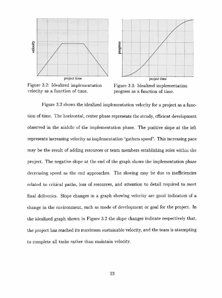
Integration of the idealized velocity for a project produces idealized progress

as a function of time (pt).

'2i„

Pt= { oL n oLp^

0<t<t^

Ljy ^ ^ 1/ ^v. LQ (3.2)

{t'^ -2tet+t^+tpte-tptg)

' 2{tg-te) S^ n// /\ '-, tq <t <te

Figure 3.3 shows an idealized implementation progress curve as a function of time.

Equation 3.2 gives the implementation progress as a function of time. Progress is

measured in accumulated metric change to date, such as total lines of code changed.

Equation 3.2 is given in terms of the previously defined parameters.

24

The proposed model is consistent with ideas proposed by others. Schneidewind

suggests artifact metric trends may be used to study the stability of the development

process (Schneidewind 1999). He defines process stability as continued improvement

in an artifact metric over time. This relationship between artifact metrics and process

metrics is stated clearly by Woodings and Bundell. They assert the derivative with

respect to time of a valid product metric is a valid process metric (Woodings and

Bundell 2001). The product metric, in the proposed model, is any size-related measure

of code. The derivative of size is growth or implementation velocity, a measure of the

implementation process.

3.3 Model Interpretive Value

Time-series data sets are rich sources of raw data. However, the metric data

itself does not directly characterize the project progress. Trends within a data set

contain much of the global meaning (DeMarco 1982; Schneidewind 1999). Extracting

meaning from this data remains difficult due to noise inherent in both the sampUng

mechanism and the process being measured. Extracting meaningful information from

the data relies on a belief about or understanding of the process which produced it

and its essential variables. The model allows the process data to be interpreted.

Or, in other words, any modelling is an interpretation of the principle mechanisms

operating within the process.

25

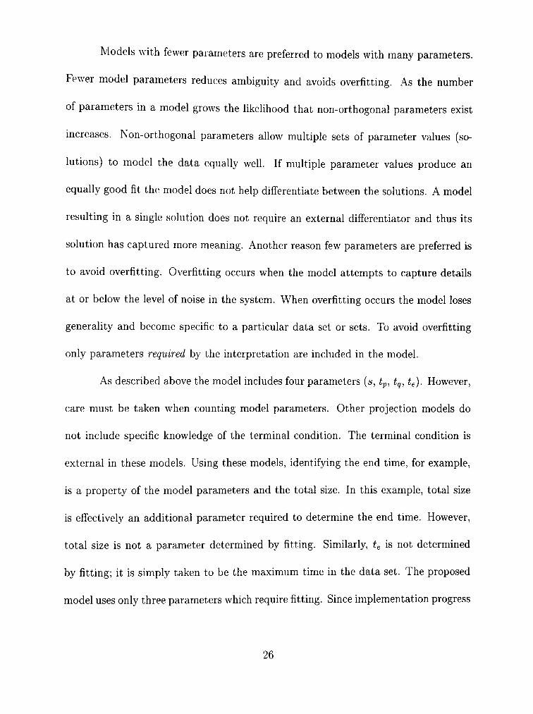
Models with fewer parameters are preferred to models with many parameters.

Fewer model parameters reduces ambiguity and avoids overfitting. As the number

of parameters in a model grows the likelihood that non-orthogonal parameters exist

increases. Non-orthogonal parameters allow multiple sets of parameter values (so­

lutions) to model the data equally well. If multiple parameter values produce an

equally good fit the model does not help differentiate between the solutions. A model

resulting in a single solution does not require an external differentiator and thus its

solution has captured more meaning. Another reason few parameters are preferred is

to avoid overfitting. Overfitting occurs when the model attempts to capture details

at or below the level of noise in the system. When overfitting occurs the model loses

generality and become specific to a particular data set or sets. To avoid overfitting

only parameters required by the interpretation are included in the model.

As described above the model includes four parameters (s, tp, tq, tg). However,

care must be taken when counting model parameters. Other projection models do

not include specific knowledge of the terminal condition. The terminal condition is

external in these models. Using these models, identifying the end time, for example,

is a property of the model parameters and the total size. In this example, total size

is eflFectively an additional parameter required to determine the end time. However,

total size is not a parameter determined by fitting. Similarly, t^ is not determined

by fitting; it is simply taken to be the maximum time in the data set. The proposed

model uses only three parameters which require fitting. Since implementation progress

26

has been seen to be both convex and concave, three parameters can be considered a

minimum parameter set.

A model expressing results in concrete units provides better insight than an

otherwise similar model using arbitrary or ambiguous units. The proposed model

does not include any scaling factors, constants, or other arbitrary parameters. The

proposed model uses only two units: time and metric-change. Both time and metric-

change are well-know units, understandable, and have obvious meaning to both de­

velopers and managers. An intuitive understanding of the units, time and metric-

change, allows tftem to be easily used in planning and evaluation. Because they are

well-known, they require no special experience or "rules of thumb" normally associ­

ated with scaling factors, constants and other invented parameters. By using concrete

units the model results may be easily related back to the project. This allows the

results to be directly used to advice management about the project.

The proposed progress model helps answer speed and estimation questions.

The model parameters can be directly used to answer management questions about

project size and the speed of development. By providing a solution in readily usable

form, predictions for "what if" scenarios are easily computed.

The proposed model allows for project implementation comparisons. Models

allow data collected from different projects to be compared. Results from the same

model applied to different data sets can be compared, revealing differences in the

projects. A model also allows projects to be compared across time or under different

27

circumstances. As more project results become available, historic basehnes can be de­

veloped. Eventually canonical profiles for each set of circumstances can be produced.

Profiles, baselines and the ability to compare projects allow better predictions to be

made.

3.4 Data Requirements

Before project implementation can be evaluated or compared, data about the

implementation must be collected. The implementation progress model proposed as­

sumes an appropriate measure of progress is available. Ideally this measure would

report "effort expended wisely", "real progress made", or even "percent of work com­

pleted". Unfortunately these highly-desirable metrics are not available. Instead, a

surrogate measure is used with the knowledge that the dimension sampled is not the

actual quantity desired (Fenton 1991). In this case, the quantity sought is imple­

mentation progress. Choosing an accurate surrogate measure of progress depends on

one's definition of progress. It may seem tempting to include all activities involved

in implementation when defining this dimension. However, the many activities re­

quired during implementation are quite diverse. This diversity is so large that the

only measures they have in common are time (or money) required to complete them.

Measuring resources expended is valuable because it allows results (progress) to be

compared with expenses. In order to allow this comparison, resource measurements

must be independent from progress measurements.

28

All of the diverse implementation activities contribute to progress in their

own way. Measuring each activity may be possible, but this approach does not easily

produce a consolidated measure unless the individual metrics are summed. Summing

many different metrics is fraught with problems such as identifying all components

and determining the correct weights for each. To avoid defining a progress metric

as the sum of many others, we define implementation progress in terms of the one

absolutely required engineering artifact necessary to deliver a software project: code.

Here we define implementation progress as a measure of the total effort captured in

deliverable code. For environments and phases that emphasize code as the primary

engineering delivery, this is an appropriate definition.

Limiting the search for a metric to an accurate measure of captured effort

within code still leaves a difficult task. Many code metrics and variations have been

proposed. A review of methods for quantifying software change covering many differ­

ent research areas concludes: "the most practical, successful measures to date appear

to be based on simple atomic counts" (Powell 1998, page 14). Even restricting a

search to "simple atomic count" metrics leaves many options. Many of the metrics

available today are primarily used for static analysis. For example, they may be used

to predict the probability that a module contains a fault rather than the total amount

of effort required to create it.

This study is interested in measuring progress in implementation artifacts.

Progress was measured as artifact change over time. Existing units of internal change

29

were unavailable, so an appropriate unit was developed. Implementation artifact

metrics traditionally used to statically measure size form the basis of the metrics

used in this study. Since this study was interested in evaluating change as a function

of time, the difference between consecutive samples was used. The change metric

is defined as the absolute difference between consecutive samples of a size metric.

This represents the change in the dimension of the size metric over the time interval

between samples. Equation 3.3 shows Am,t is the change in a metric m at time t.

Am,t = \mt - mt-i\ (3.3)

The absolute value of each difference was used. This assumes that the correct

removal of code artifacts was approximately as challenging as correctly adding the

code. This point could be contested by those claiming that removing code is easier

than adding code. While that may be true, it cannot be claimed that the removal

effort represents progress away from the goal, which would be the case if "negative

effort" was permitted. To avoid introducing a weighting factor for "negative" changes,

all changes were treated equally. These new metrics measure the size of change over

the sample interval, or in other words, they give a measure of implementation progress.

Existing artifact measures shown to be related to size were chosen for this

study. Chapter IV discusses the specific details of each metric used.

30

3.5 Data Collection

In a team environment, software implementation occurs in parallel as each

team member works semi-independently. From the perspective of the project source

repository, development occurs simultaneously across many source files. This chaotic

environment means capturing progress for a complete project requires summing the

change from many individual source files. Similarly, multiple changes within a single

file are accumulated to find the total change across the time interval of interest.

Collecting measurements of implementation change would typically be done as

each source file was submitted to the project source repository. This mechanism helps

provide part of the "real-time" data needed to manage the project. For this study,

"live" projects were not available, however project source repositories with version-

control were available. These source repositories allow source files to be retrieved for

any point in the history of the project. By retrieving each version of a file, a time-

stamped series of intermediate files can be collected. This retroactive recovery of each

version means the data collected is equivalent to what would have been collected

"live" during the project implementation phase. For each version of a source file,

the following pieces of raw data were collected: date and time, filename, version

number, submission engineer, and the various effort metrics discussed in the next

chapter. Additional derived pieces of data were computed including elapsed time

in project, elapsed time since the file last changed, and other files submitted at the

"same" time. Files were determined to be submitted at the "same" time if the same

31

author submitted both files and the recorded submission times differed by at most

three minutes.

Several of the project data sets contained anomalies which were judiciously

removed. Six of the data sets included unusual entries long after the completion date

for the project. In some cases, this was evidently a mistaken submission of a file to the

wrong repository. In other cases, this was evidence that a later, minor maintenance

release of the project was produced. A gap of at least one month in the data was

used to identify the end of the project. A future work may compare these projects

against those without revisions to determine if the projects were shipped "too soon".

In addition to outliers near the end of the data set, three projects contained unusual

events related to repository submissions. In two cases, a zero-length file was submitted

to the repository immediately before being resubmitted correctly. In one case, several

hundred lines of code were removed from a file only to be immediately added to

another file. These three data events were considered to be the result of misuse of

the repository and the events were removed. Finally, project one was discovered to

included a prototype phase. Since the engineering team changed following completion

of the prototype, it was treated as two projects (la and lb).

3.6 Data Source

Seventeen projects from a single company were studied. All projects were de­

veloped using the same process. They were six weeks to eighteen months in length and

32

involved one to eight engineers. All projects produced multimedia software designed

to be marketed to consumers for use with Microsoft® Windows® and on Macintosh®

personal computers between 1995 and 2002. Much of the total project effort for these

projects was not software development but rather multimedia content development.

Source and content development outside the usual definition of software was not con­

sidered; only source files created by software engineers and containing source code

was included in the study.

The projects studied were not on-going efforts such as the more typical sce­

nario of software maintained for in-house use. The projects were intended for mass-

distribution to consumers, maintenance changes were not anticipated or economically

acceptable. Clear delivery dates exist after which no work was to be done. This is

unlike some other environments, where software is deployed rather than delivered,

and implementation evolves into a continuous cycle of maintenance. The progress

model studied is expected to be meaningful when applied to each release of on-going

projects, however additional studies will be needed to establish this. Results from

this homogeneous group of projects should apply to initial development efforts of all

projects and to projects without maintenance phases.

33

CHAPTER IV

EFFORT METRICS

Three established metrics were used in the study. Two variations on the lines

of code metric were considered. Also included are Halstead's volume measure and

McCabe's cyclomatic complexity measure. These metrics have been studied together

many times. Several studies showing the correlation with effort or faults have been

published using these metrics (Lind and Vairavan 1989; Kafura and Canning 1985).

Each of the metrics is described below including definition, references, and details

about implementation within the study. Measures other than those studied here

could be used and several suggestions for future investigation are included below.

These additional metrics are not be included in this initial study.

4.1 Source Lines of Code

Software size can be measured using a count of source lines of code (SLOG)

contained within the project. This metric includes many variations. The Software

Engineering Institute has identified dozens of issues that should be considered when

defining SLOC (Park 1992). These issues help define what exactly counts as a line

of code. Typically lines containing only white space and lines consisting of comment

characters without any alphabetic characters are not counted. In addition to the

preceding rule, physical lines containing both code and comments count as two lines

for this study.

34

While some researchers continue to dismiss SLOC as a poor measure (Lehman,

Ramil, Wernick, and Perry 1997), studies have shown strong correlations between

SLOC and other properties such as effort, project duration, and quahty. Lind and

X' airavan even show it can outperform more complex measures (Lind and Vairavan

1989). One of the main arguments against this metric is its susceptibility to "spoof­

ing". For example, simply using a different formatting scheme will produce different

results. Other intentional spoofing effects are even easier to imagine. In this case,

since the data was collected after the fact, the project engineers had no knowledge of

this study. Lacking knowledge of the study and since no measurements were taken or

published within the development environment, intentional spoofing effects are not

possible. Mitigating unintentional counting effects relies on consistent coding prac­

tices or standards. In this case, the development environment strongly encouraged

conformance to a consistent set of coding standards. Since similar coding standards

were in effect for all projects, unintentional effects should be mitigated. In general,

strong conformance with local standards should improve the quality of this type of

metric.

New studies continue to cite SLOC as an independent variable for various

studies. Its continued use has been attributed to its use as the null hypothesis of

measures by Powell (Powell 1998). It is also regularly used to estimate projects

and measure productivity. These studies and estimates substitute a specific SLOC

metric for a true measure of the desired dimension. For example, Schneidewind uses

35

lines of code changed as a measure of total effort in his study of process stability

(Schneidewind 1999). Jorgensen uses lines of code changed to measure maintenance

task size in his study of maintenance task prediction models (Jorgensen 1995).

This study will consider two variations of SLOC. The simplest form counts the

SLOC change (SLOCC) for each file submitted. SLOCC is the absolute difference

in SLOC between source files consecutively submitted to the repository. That is, it

counts SLOC added or deleted from the previous version. The second form measures

the number of lines actually changed between submissions by comparing the files.

This second measure is sometimes referred to as code churn (CHURN) (El-Eman

2000). CHURN is the count of source lines inserted, deleted, or changed between

source files consecutively submitted to the repository. It is probably a better metric

than SLOCC since CHURN captures changed lines (which also represent real work

based on arguments presented above) that are not captured by SLOCC alone.

4.2 McCabe Complexity

The second software size metric considered uses cyclomatic, or McCabe, com­

plexity measure (MCM) as its basis (McCabe 1976). For a single function, cyclomatic

complexity can be computed by adding one to the count of flow-control decision

points. For several functions, its value is the count of all decision points plus the

count of functions under consideration. This study used this definition and grouped

functions by the source file in which they appeared.

36

MCM was originally proposed as an complexity evaluator of functions or mod­

ules. MCM was invented before object-oriented development was available, so it only

considers algorithmic size, not structural or object size. It has been studied almost as

extensively as SLOC and many studies have shown that MCM and SLOC are highly

correlated (Lake and Cook 1994; Lind and Vairavan 1989). Based on this reasoning,

Andersson et al argue cyclomatic complexity is actually a measure of effort (Ander-

sson, Enholm, and Torn ). They define effort as program length times real average

complexity {effort = length x complexity). They demonstrate cyclomatic complexity

captures the product of the length dimension and the hidden dimension of real com­

plexity. This finding indicates a measure based on MCM could provide an acceptable

surrogate for captured effort.

This study considers changes in MCM to represent a measure of effort re­

quired to achieve the change. This McCabe complexity change (MCC) is defined as

the absolute difference between MCM values of source files consecutively submitted

to the repository. Ideally, several variations on this metric would be considered. For

example, the MCM of the actual lines added, deleted, or changed. This measure is

conceptually similar to the difference between SLOCC and CHURN. Another inter­

esting metric to consider is the sum of the complexity of all functions changed. This

suggestion assumes that any change to a function requires at least some understanding

of the entire function.

37

4.3 Halstead Volume

The third software size metric considered uses Halstead's Software Science

measure of program implementation length (Halstead 1977). Halstead implemen­

tation length (HIL) is defined as the total of operator count and operand count.

Halstead defines operands as variables and constants; he defines operators as com­

binations of symbols that affect the value or ordering of an operand. From these

definitions and his example it is obvious that HIL varies only slightly from a count

of tokens. Halstead does not provide a precise definition of operator or operands

for the C++ programming language. Instead of attempting to arbitrarily map C++

constructs to Halstead operands and operators, a token count was used.

Halstead defines many metrics derived from the count of operators and oper­

ands. From these he derived many more exotic Software Science metrics. Debate

continues as to the theoretical and empirical validity of most of these measures (Fen­

ton and Neil 1999). While many of these metrics have generally been disregarded,

his definition of implementation size remains in use for much the same reason SLOC

is used-it has an obvious meaning in most contexts and is easy to implement, esti­

mate and understand. Albrecht studied the use of Halstead's implementation length

estimate and function points as a tool for estimating projects (Albrecht and John

E. Gaffney 1983). He shows that for large projects estimated functions points can be

used to predict HIL, which can be used to predict SLOC and implementation time.

38

One Software Science metric with potential appeal for this study is program­

ming effort. Halstead describes programming effort as "the mental activity required

to reduce a preconceived algorithm to an actual implementation in a language in

which the implementor (writer) is fluent" (Halstead 1977, page 46). Unfortunately

this definition is more restrictive than what we desire in that it does not include time

to "concei\'e" the algorithm but rather seems to predict the time required to simply

enter the code.

This study considers changes in HIL to represent a measure of the effort re­

quired to achieve the change. Halstead length change (HLC) is defined as the absolute

difference between HIL values of consecutive source files submitted to the repository.

Like the McCabe measures, ideally several other measures would be studied as well.

For example, the sum of HIL for the fines actually changed seems appropriate. As

above, this is based on the reasoning that changes in a line of code require an un­

derstanding of at least that whole line. A similar argument can be made for the

containing function, and to a lesser extent the containing class or module. Halstead

also defines program volume in terms of the number of bits required to store it. Dif­

ferences between total volume, rather than size, could be considered. Attempting to

measure the volume of the current change could also be studied.

39

4.4 Other Metrics

The metrics selected for this study were chosen by a combination of factors

including demonstrated utility and practicality. Other metrics could have been chosen

and clearly they will need to be studied. For example, Lehman et al use module count

as a surrogate for size in their study of software evolution (Lehman, RamU, Wernick,

and Perry 1997). Several other interesting metrics suspected of providing high-quality

measures are described below.

One area of software size without an established and simple measure is that

of object-oriented code. Lake and Cook show that MCM and SLOC alone miss at

least one major dimension of object-oriented software (OOS) (Lake and Cook 1994).

Using component analysis they show OOS has a dimension related to the number

of classes, number of polymorphic functions, and number of inheritance fines. Their

analysis did not address complete systems, only class trees and individual classes.

Defining and evaluating a metric based on object-oriented attributes such as those

listed above seems promising. A simple, practical measure for the extra dimension(s)

found in OOS would be very useful.

Henry and Kafura created and studied a metric based on information flow

(Henry and Kafura 1981). This measure might provide a better measure of overall

size or complexity for OOS than the existing ones. However, it does not specifically

attempt to capture size or effort. It is also extremely complex to implement, so for

these reasons it was not included in this study.

40

One other metric which could be considered is inspired by Strelzoff (Strelzoff

and Petzold 2003). He uses differences in Huffman compression (Huffman 1952) as

a surrogate for the information distance between two versions of program source

code. A similar algorithm could be used to generate a potentially better size-change

metric. This is especially true if the differences, rather than the complete source,

were compressed using only the dictionary of the original source. This process would

give the information distance for the change.

41

CHAPTER V

RESULTS

Parameterized models provide an approximation of the sampled data for a

particular data set. From a quantitative perspective, the model curve which most

closely fits the data is considered the best, since it introduces the least error. Model

fit can be measured using the squared residual after subtracting the model curve

from the sample data. To allow comparisons between data sets the average squared

residual error {R^) is usually used. Large values of R'^ indicate the model does not

fit the data. When comparing models, the model with the lowest R^ for a particular

data set provides the closest approximation. In order to establish that a model is

generally better, similar results should be obtained from multiple data sets covering

the domain of interest.

5.1 Alternative Models

In addition to the proposed implementation progress model, three alternative

models were chosen to provide a context for evaluating the fit of the proposed model.

The usual quantitative analysis for a new model is to show that it performs better than

existing models. In this case, no established implementation progress model exists.

Therefore, to provide a frame of reference, three alternative models were selected for

comparative analysis.

42

The first model was a standard linear approximation. The linear model curve

is given by Equation 5.1. Linear approximation, with only two degrees-of-freedom,

represents a practical lower-bound on the number of model parameters. Alternatively,

it can be viewed as the model with the highest expected R'^. It was chosen as a

practical upper-bound on R^.

lineavt = at + b (5.1)

Of the three alternative models, linear approximation is the only model with

obvious interpretations for its parameters. The slope (a) represents the average ve­

locity. The y-intercept {b) can be interpreted as a "correction factor" necessary to

reduce error.

The second alternative model chosen was a multiphase, piecewise parabohc

approximation. It contains eleven degrees-of-freedom; its model curve is shown in

Equation 5.2. This model was chosen to represent a practical lower-bound on R^. No

suggestion is made as to the interpretation of the individual model parameters.

( at'^ + bt + c, Q<t <tp

dt^ + et + f, tp<t<tq (5.2)

\gt^ + ht + i, tq<t< te

This model was chosen to provide a reasonable lower-bound for i?^ given an

extremely data conforming model. The multiphase model equation contains the pro-

multiphaset = <

43

posed model equation as a special case. Since the proposed model consists of three

pieces, the multiphase model is piecewise with three segments as well. Where the

proposed model consists of two parabolic segments and one linear segment; the mul­

tiphase model allows three parabolic segments. The proposed model is smooth, its

first derivative is continuous; the multiphase model equation makes no such guaran­

tees.

The third model was a third-degree polynomial approximation, with four

degrees-of-freedom. The polynomial model curve is shown in Equation 5.3. A third-

degree polynomial approximation provides enough flexibility to model the s-curve

observed. It also provides a model of approximately the same degrees-of-freedom as

the proposed model. Again, no interpretation of the individual model parameters is

suggested.

polynomialt = at^ + bt'^ + ct + d (5.3)

5.2 Model Fitting Results

Evaluations of each metric for each project were performed. The three alter­

native models described above and the proposed model were used. Model parameters

were found for each to minimize R^. Representative projects are discussed below.

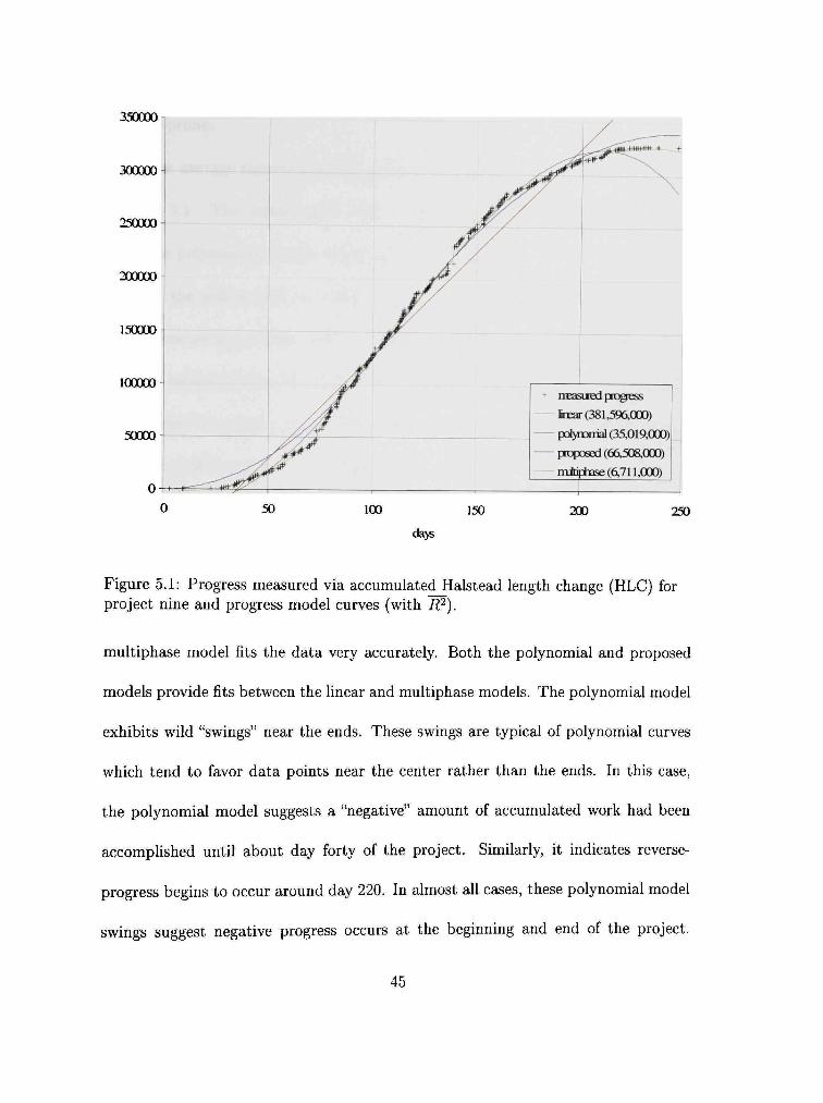
Figure 5.1 shows progress measured via accumulated HLC and model curves

for project nine. As expected, the hnear model provides a poor fit for the data and the

44

350000

300000^

250000

200000

150000

100000

50000

-i

jf.

^4 r

+ rreasued progess

Imear (381,596,000)

pQl>TOnial (35,019,000)

proposed (66,508,000)

mJtiphase (6,711,000)

50 100 150 200 250

dajs

Figure 5.1: Progress measured via accumulated Halstead length change (HLC) for project nine and progress model curves (with R^).

multiphase model fits the data very accurately. Both the polynomial and proposed

models provide fits between the hnear and multiphase models. The polynomial model

exhibits wild "swings" near the ends. These swings are typical of polynomial curves

which tend to favor data points near the center rather than the ends. In this case,

the polynomial model suggests a "negative" amount of accumulated work had been

accomplished until about day forty of the project. Similarly, it indicates reverse-

progress begins to occur around day 220. In almost aU cases, these polynomial model

swings suggest negative progress occurs at the beginning and end of the project.

45

Because of this, using the polynomial model to make predictions would be difficult

and error-prone.

The average squared residual error {R^) for each model is given in the legend

of Figure 5.1. The values agree with a visual assessment of the fit except in the

case of the polynomial model. While the lower W for the polynomial model is more

desirable, the polynomial fit suffers extensively from undesirable swings near the

ends. These swings violate a basic expectation of accumulated progress, that is it

should be monotonically increasing. While the proposed model has a larger R^, it is

monotonically increasing and behaves as expected. This behavior appears to support

in-project predictions better than the polynomial model.

In this project, most of the proposed model R'^ can be seen to occur in the first

third of the project. Each of the other three metrics show similar results; this may

indicate early efforts are not as efficiently captured by the metrics as later efforts. It

may also indicate the project pace was unpredictably high (in violation of the implied

model) during the later part of the project. Without additional information about

the project, or its context, a determination cannot be made.

Figure 5.2 shows progress measured via accumulated MCC and model curves

for project ten. In addition to the general observations noted above, two observa­

tions can be made from this graph. First, discontinuities in the multiphase model

are visibly apparent, occurring at about day thirty and 72. Discontinuities severely

reduce the predictive value of a model because no influence occurs across a disconti-

46

leoo

1400

1200

ICOO

800

600

4C0

200

o-t*±-

+ rreasiredprogESS

linear (8561)

pol>nDmal(1434)

pnopo6ed(7D6)

miliphase (324)

140

Figure 5.2: Progress measured via accumulated cyclomatic complexity change (MCC) for project ten and progress model curves (with R^).

nuity. In addition, the discontinuity locations cannot be predicted without all data.

Second, unlike project nine, R^ for the proposed model is less than half the R'^ for

the polynomial model.

Implementation progress for this project follows closely the proposed model

curve. This suggests the process used was healthy and the project was consistently

"on track". Figure 5.3 shows weekly accumulated progress measured via MCC and

the velocity model curve for the project. Directly measuring velocity is not possible

because measurements taken represent progress. Due to the sporadic nature of source

47

250

200

+ measured data

— velocity model

o _o u >

Figure 5.3: Weekly progress measured via accumulated cyclomatic complexity change (MCC) for project ten and velocity model curve.

submissions determining average velocity is difficult. Accumulated weekly progress is

used as a surrogate for velocity. Again, the model curve suggests the project was well

managed. The model indicates implementation velocity reached a sustainable level

within the first month of development. This continued for about three weeks, then

the velocity began to decrease. The relatively long deceleration period may be worth

investigating, it may indicate the project experienced trouble finishing. However,

considering the short development period, it may indicate the startup was unusually

efficient. Without additional context information a determination cannot be made.

48

25000

20000

15000

10000

5000

i

1

-

^ f

jX* J/

\

1 ^

]__ Y _,

A

r

^ ,

4*'- i

^ ^ >

• rrEasued pcogess

linear (4S4,400)

pdjmmal (468,400) , , , , ^ .jari / / w ; /inn\ proposeu ('HUCJ.'HOU) inJtiphase (81,400)

1 1 ; 20 40 60 80 100

da>s

120 140 160 180

Figure 5.4: Progress measured via accumulated code churn (CHURN) for project fifteen and progress model curves (with R^).

5.3 Anomalous Data Sets

Results from some data sets were ambiguous. For example. Figure 5.4 shows

progress measured via accumulated CHURN and model curves for project fifteen.

Neither the polynomial nor the proposed model provides a significant improvement

over the linear model. Numerically, the multiphase model is significantly better than

the others, however it suffers extensively from a discontinuity around day fifty.

It is worth noting the large gaps in collected data around days fifteen and

fifty, and the periodic gaps of one to two days near the beginning of the project.

49

4000-

3500

3000

2500

2000

1500

1000^

500

0 ^

50 100

da>s

+ measired ppqgtss

linear (9837)

— polynDmal (6566)

— proposed (8341)

mitiphase(1759)

150 200

Figure 5.5: Progress measured via accumulated cyclomatic complexity change (MCC) for project four and progress model curves (with R'^).

A closer look at the raw data shows the periodic gaps occur on weekends and the

larger gaps correspond to Thanksgiving and Christmas holidays respectively. It is

reasonable to assume no work was done during those times. Unfortunately, employee

billing information is not available for the project so this cannot be confirmed.

Figure 5.5 shows progress measured via accumulated MCC and model curves

for project four. Again, the multiphase model provides a substantial improvement

over the other models. In this case, the polynomial model reduces R^ by about

one-third, but the proposed model gives a smaller improvement.

50

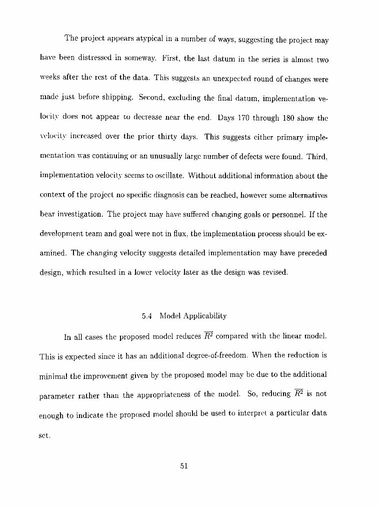
The project appears atypical in a number of ways, suggesting the project may

have been distressed in someway. First, the last datum in the series is almost two

weeks after the rest of the data. This suggests an unexpected round of changes were

made just before shipping. Second, excluding the final datum, implementation ve­

locity does not appear to decrease near the end. Days 170 through 180 show the

velocit}' increased over the prior thirty days. This suggests either primary imple­

mentation was continuing or an unusually large number of defects were found. Third,

implementation velocity seems to oscillate. Without additional information about the

context of the project no specific diagnosis can be reached, however some alternatives

bear investigation. The project may have suffered changing goals or personnel. If the

development team and goal were not in flux, the implementation process should be ex­

amined. The changing velocity suggests detailed implementation may have preceded

design, which resulted in a lower velocity later as the design was revised.

5.4 Model Applicability

In all cases the proposed model reduces R'^ compared with the linear model.

This is expected since it has an additional degree-of-freedom. When the reduction is

minimal the improvement given by the proposed model may be due to the additional

parameter rather than the appropriateness of the model. So, reducing R'^ is not

enough to indicate the proposed model should be used to interpret a particular data

set.

51

On the other hand, in many cases the proposed model substantially reduces

R^ when compared with a linear model. In a few of these cases the reduction in W is

almost to the level achieved using the multiphase model. In these conforming cases

the proposed model provides a meaningful interpretation of the data.

The i?2 for eacli metric is given in Tables 5.1 through 5.4. Figures 5.6 through

5.9 show i?2 relative to the linear model R~ for each project. To improve viewing

projects are ordered by polynomial model relative R'^.

Consider the proposed model i?^ compared with the linear model i?^. In cases

where the proposed model substantially reduces R'^, the model gave improved results

with the addition of a single parameter. This substantial improvement suggests the

data conforms to the model and the results may be relied upon to correctly interpret

the data. That is, it is reasonable to assume the flt parameters (s, tp, and tq) are a

true representation of implementation progress for the project. In the non-conforming

cases, where the reduction is less significant, the model may not be appropriate and

the results should only be used judiciously. Based on the available projects, the

author suggests that the proposed model may be relied upon when the R^ is at most

half that of the linear model.

Projects may be non-conforming due to noise in the metric data. Almost

all projects exhibit noticeable one to two day "pauses". These are especially common

during the first haff of each project and repeat with a seven-day period. Some projects

also include larger periods when no apparent progress is made during a holiday break.

52

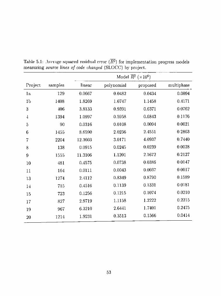
Table 5.1: Average squared residual error (i?^) for implementation progress models measuring source lines of code changed (SLOCC) by project.

Project

la

lb

3

4

5

6

7

8

9

10

11

13

14

15

17

19

20

samples

129

1408

406

1394

90

1455

2204

138

1555

481

164

1274

715

723

827

967

1214

linear

0.0667

1.8269

3.8133

1.0997

0.0316

8.6590

12.3603

0.0915

11.3106

0.4575

0.0111

2.4112

0.4516

0.1256

2.9719

6.3210

1.9231

Model i?2

polynomial

0.0482

1.6747

0.9391

0.5958

0.0108

2.0236

3.0171

0.0245

1.1201

0.0738

0.0043

0.8349

0.1139

0.1215

1.1158

2.6441

0.3513

(xlO^)

proposed

0.0434

1.1458

0.6371

0.6843

0.0094

2.4551

4.0937

0.0239

2.1672

0.0386

0.0037

0.8790

0.1331

0.1074

1.2222

1.7401

0.1566

multiphase

0.0094

0.4171

0.0762

0.1176

0.0021

0.2863

0.7440

0.0028

0.2127

0.0147

0.0017

0.1589

0.0181

0.0210

0.2215

0.2475

0.0414

53

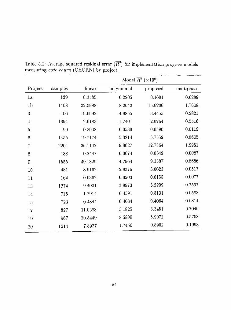
Table 5.2: Average squared residual error {R^) for implementation progress models measuring code churn (CHURN) by project.

Project

la

lb

3

4

5

6

7

8

9

10

11

13

14

15

17

19

20

samples

129

1408

406

1394

90

1455

2204

138

1555

481

164

1274

715

723

827

967

1214

linear

0.3485

22.0988

19.6692

2.6183

0.2008

19.7174

36.1142

0.2487

49.1829

8.9162

0.0362

9.4001

1.7914

0.4844

11.0583

20.5449

7.8927

Model i?2

polynomial

0.2205

8.2642

4.9855

1.7401

0.0530

5.3214

9.8627

0.0674

4.7964

2.8376

0.0203

3.9973

0.4591

0.4684

3.1825

8.5899

1.7450

(xlO^)

proposed

0.1601

15.6206

3.4455

2.0264

0.0590

5.7359

12.7864

0.0549

9.3587

3.0023

0.0155

3.2209

0.5131

0.4064

3.3451

5.9072

0.8902

multiphase

0.0289

1.7608

0.2821

0.5516

0.0119

0.8605

1.9951

0.0087

0.8686

0.0517

0.0077

0.7597

0.0593

0.0814

0.7040

0.5758

0.1993

54

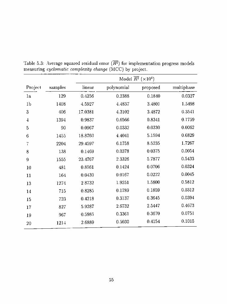
Table 5.3: Average squared residual error (i?^) for implementation progress models measuring cyclomatic complexity change (MCC) by project.

Project

la

lb

3

4

5

6

7

8

9

10

11

13

14

15

17

19

20

samples

129

1408

406

1394

90

1455

2204

138

1555

481

164

1274

715

723

827

967

1214

linear

0.4256

4.5927

17.0381

0.9837

0.0967

18.8760

29.4597

0.1469

23.4767

0.8561

0.0430

2.8732

0.8285

0.4218

5.9287

0.5985

2.6889

Model i?2

polynomial

0.2388

4.4837

4.3102

0.6566

0.0332

4.4041

6.1758

0.0378

2.3326

0.1424

0.0167

1.9251

0.1789

0.3137

2.6732

0.3361

0.5030

(xlO^)

proposed

0.1840

3.4801

3.4872

0.8341

0.0330

5.1594

8.5235

0.0375

5.7877

0.0706

0.0222

1.5800

0.1859

0.3645

2.5447

0.3670

0.4154

multiphase

0.0327

1.5498

0.3541

0.1759

0.0062

0.6829

1.7267

0.0054

0.5433

0.0324

0.0045

0.5812

0.0312

0.0394

0.4673

0.0751

0.1015

55

Table 5.4: A\erage squared residual error {R^) for implementation progress models measuring Halstead length change (HLC) by project.

Project

la

lb

3

4

5

6

7

8

9

10

11

13

14

15

17

19

20

samples

129

1408

406

1394

90

1455

2204

138

1555

481

164

1274

715

723

827

967

1214

linear

0.2576

4.8578

9.6200

1.1556

0.0721

26.8214

45.4181

0.3707

38.1596

1.4100

0.0316

3.3893

2.1188

0.4676

7.6514

8.3263

3.9044

Model i?2

polynomial

0.1478

3.9031

2.5890

0.8592

0.0232

6.3090

13.1349

0.0945

3.5019

0.2470

0.0103

1.1128

0.6570

0.4521

3.8954

3.8056

0.7697

(xlO^)

proposed

0.1036

2.7345

1.7247

0.9446

0.0260

7.6396

16.5184

0.0902

6.6508

0.1229

0.0103

0.9574

0.8304

0.3730

3.5683

3.7480

0.5633

multiphase

0.0170

1.1013

0.1905

0.2056

0.0067

0.8003

2.8797

0.0097

0.6711

0.0521

0.0043

0.3244

0.0895

0.0812

0.6345

0.3882

0.1198

56

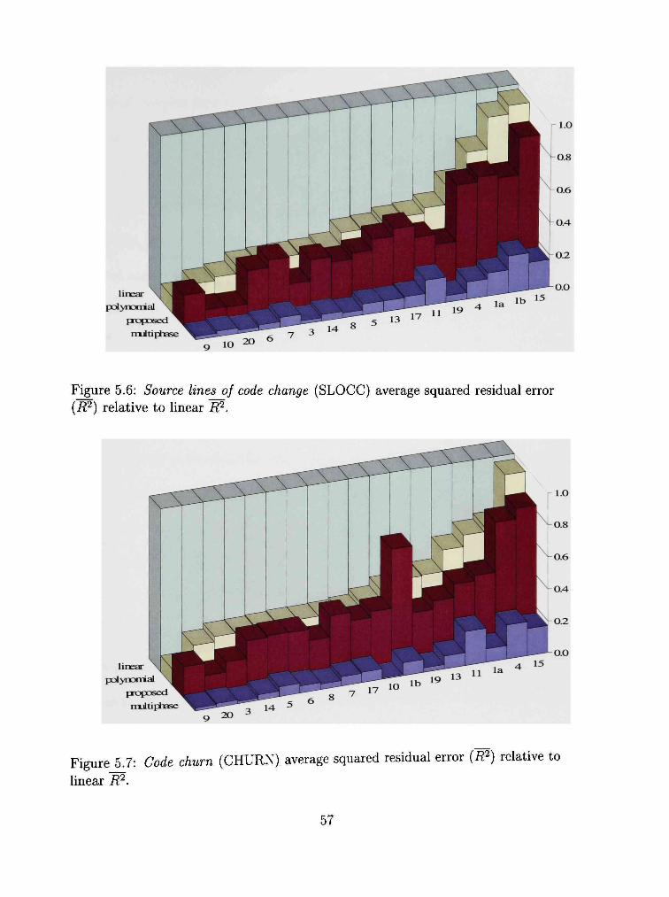
linear polynomial

proposed ni t iphase

l.O

0.8

0.6

0.4

0.2

0.0

Figure 5.6: Source lines of code change (SLOCC) average squared residual error (i?2) relative to linear R^.

linear polynomial

proposed mjiti phase

l.O

0.8

0.6

0.4

0.2

0 .0

Figure 5.7: Code churn (CHURN) average squared residual error {R^) relative to

linear R^.

57

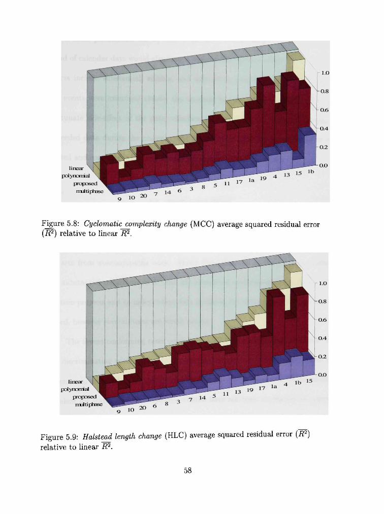
1.0

-0 .8

0.6

0.4

0.2

O.O

Figure 5.8: Cyclomatic complexity change (MCC) average squared residual error (i?2) relative to linear /?2

linear polynorrial

proposed nxltiphase

Figure 5.9: Halstead length change (HLC) average squared residual error {R^)

relative to linear R"^.

58

Both of these phenomena can be seen in projects la and fifteen. Using work days

instead of calendar days would eliminate a major cause of time-related noise. Several

projects include substantial, sudden, and anomalous progress. In all cases where

these events were examined closely, the anomaly has proven to be the result of an

unfortunate side-effect of the data collection procedure. A commitment to collect

the needed data during the project could reduce noise by allowing anomalies to be

detected and corrected while any needed information is still available.

5.5 Conforming Cases

Tables 5.5 through 5.8 show the model parameters for each project and met­

ric. Projects are ordered by i?2 relative to linear 'W and a line divides conforming

data sets from nonconforming ones. About three-quarters of the projects studied

show substantial reductions in R^ and are considered conforming cases. With only

seventeen projects and no independent data available, few definite conclusions can be

reached, however several items are worth noting.

The fewest conforming cases occur in Table 5.7, indicating that MCC may be

more discriminating with respect to implementation progress. This is likely due to

differences in emphasis. All the metrics studied have been shown to be essentially

equivalent for static analysis. However, studies have not been conducted on typical

change of these metrics over time. Consider that MCC counts entry points (functions)

59

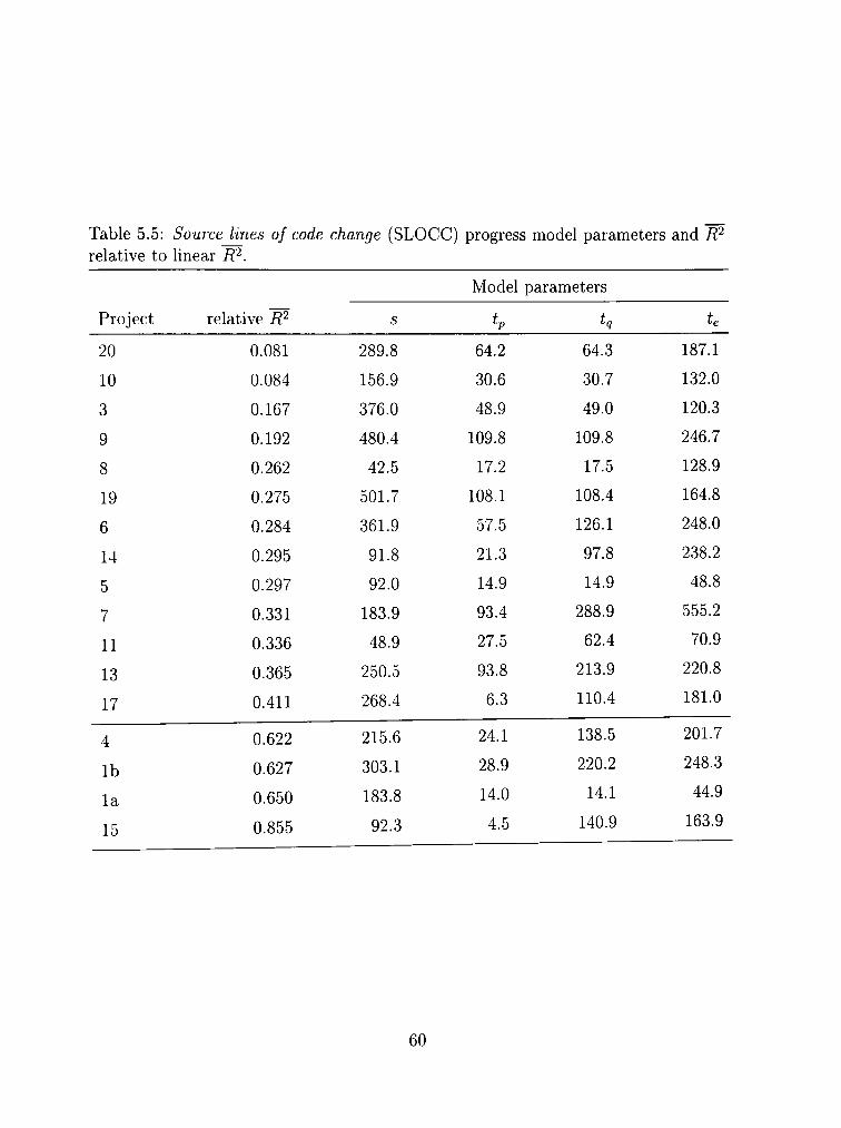
Table 5.5: Source lines of code change (SLOCC) progress model parameters and R^ relative to linear R^.

Project

20

10

3

9

8

19

6

14

5

7

11

13

17

4

lb

la

15

relative R^

0.081

0.084

0.167

0.192

0.262

0.275

0.284

0.295

0.297

0.331

0.336

0.365

0.411

0.622

0.627

0.650

0.855

s

289.8

156.9

376.0

480.4

42.5

501.7

361.9

91.8

92.0

183.9

48.9

250.5

268.4

215.6

303.1

183.8

92.3

Model parameters

Lp

64.2

30.6

48.9

109.8

17.2

108.1

57.5

21.3

14.9

93.4

27.5

93.8

6.3

24.1

28.9

14.0

4.5

k 64.3

30.7

49.0

109.8

17.5

108.4

126.1

97.8

14.9

288.9

62.4

213.9

110.4

138.5

220.2

14.1

140.9

te

187.1

132.0

120.3

246.7

128.9

164.8

248.0

238.2

48.8

555.2

70.9

220.8

181.0

201.7

248.3

44.9

163.9

60

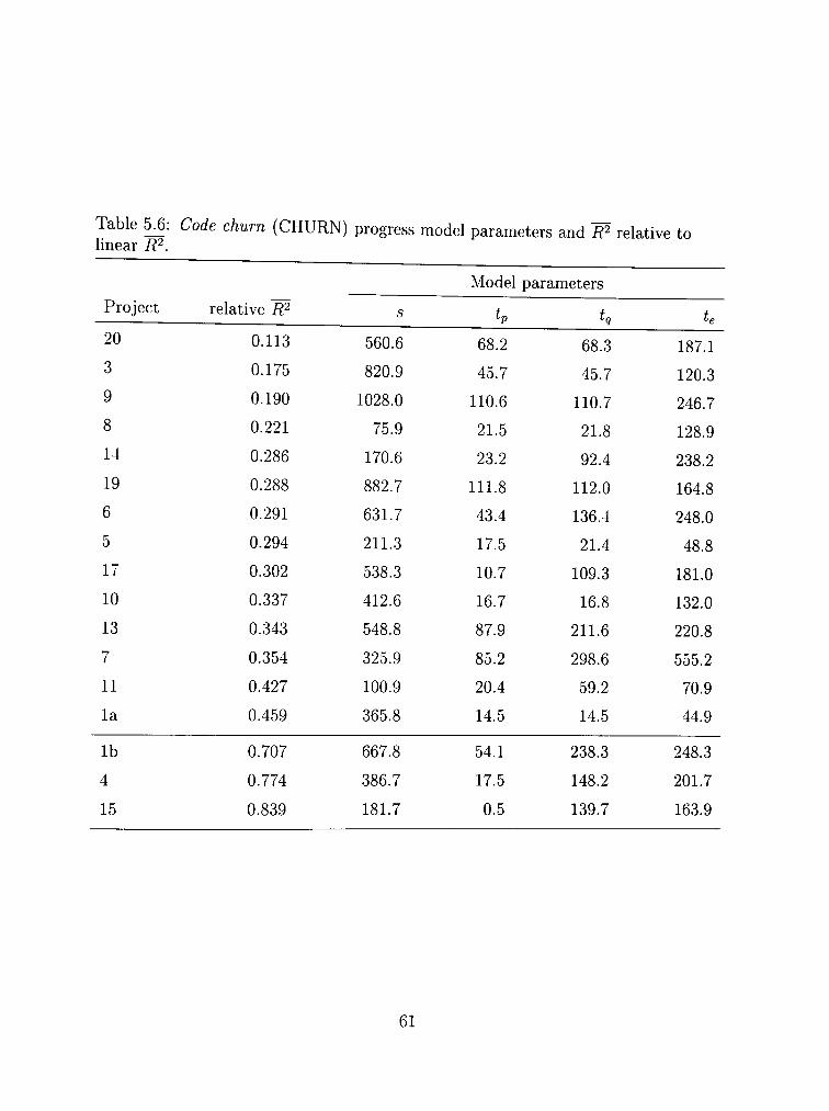
Table 5^: Code churn (CHURN) progress model parameters and ^ relative to linear R^.

Project

20

3

9

8

14

19

6

5

17

10

13

7

11

la

lb

4

15

relative R^

0.113

0.175

0.190

0.221

0.286

0.288

0.291

0.294

0.302

0.337

0.343

0.354

0.427

0.459

0.707

0.774

0.839

s

560.6

820.9

1028.0

75.9

170.6

882.7

631.7

211.3

538.3

412.6

548.8

325.9

100.9

365.8

667.8

386.7

181.7

Model

tp

68.2

45.7

110.6

21.5

23.2

111.8

43.4

17.5

10.7

16.7

87.9

85.2

20.4

14.5

54.1

17.5

0.5

parameters

t.

68.3

45.7

110.7

21.8

92.4

112.0

136.4

21.4

109.3

16.8

211.6

298.6

59.2

14.5

238.3

148.2

139.7

te

187.1

120.3

246.7

128.9

238.2

164.8

248.0

48.8

181.0

132.0

220.8

555.2

70.9

44.9

248.3

201.7

163.9

61

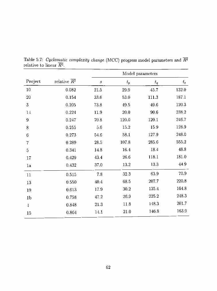
Table 5.7: Cyclornatic complexity change (MCC) progress model parameters and R^ relative to linear i?^

Project

10

20

3

14

9

8

6

7

5

17

la

11

13

19

lb

4

15

relative R'^

0.082

0.154

0.205

0.224

0.247

0.255

0.273

0.289

0.341

0.429

0.432

0.515

0.550

0.613

0.758

0.848

0.864

s

21.5

33.6

73.8

11.9

70.8

5.6

54.6

28.5

14.8

43.4

37.0

7.8

40.4

17.9

47.2

21.3

14.1

Model

Zp

29.9

53.0

49.5

20.0

120.0

15.2

58.1

107.8

16.4

26.6

13.2

32.3

68.5

30.2

26.9

11.8

21.0

parameters

t.

45.7

111.3

49.6

90.6

120.1

15.9

127.9

285.6

18.4

118.1

13.3

63.9

207.7

135.4

225.2

148.3

146.8

te

132.0

187.1

120.3

238.2

246.7

128.9

248.0

555.2

48.8

181.0

44.9

70.9

220.8

164.8

248.3

201.7

163.9

62

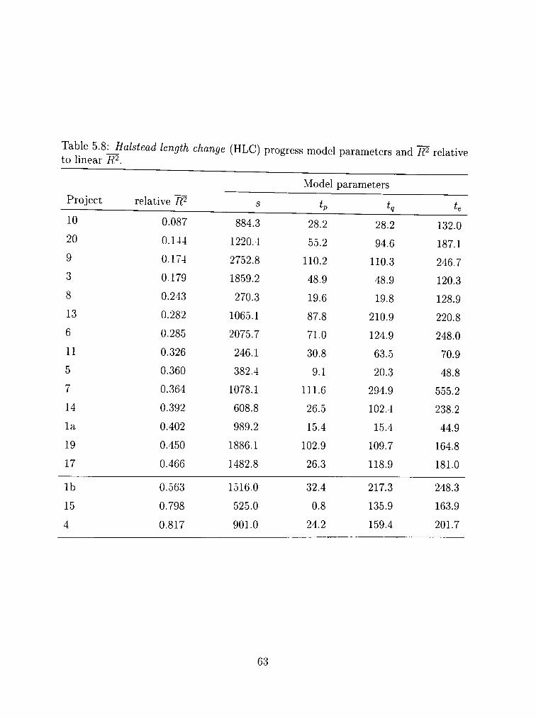
Table 5.8-JIalstead length change (HLC) progress model parameters and W relative to linear R^.

Project

10

20

9

3

8

13

6

11

5

7

14

la

19

17

lb

15

4

relative R'^

0.087

0.144

0.174

0.179

0.243

0.282

0.285

0.326

0.360

0.364

0.392

0.402

0.450

0.466

0.563

0.798

0.817

s

884.3

1220.4

2752.8

1859.2

270.3

1065.1

2075.7

246.1

382.4

1078.1

608.8

989.2

1886.1

1482.8

1516.0

525.0

901.0

Model

Zp

28.2

55.2

110.2

48.9

19.6

87.8

71.0

30.8

9.1

111.6

26.5

15.4

102.9

26.3

32.4

0.8

24.2

parameters

t,

28.2

94.6

110.3

48.9

19.8

210.9

124.9

63.5

20.3

294.9

102.4

15.4

109.7

118.9

217.3

135.9

159.4

te

132.0

187.1

246.7

120.3

128.9

220.8

248.0

70.9

48.8

555.2

238.2

44.9

164.8

181.0

248.3

163.9

201.7

63

and decision points, while tlie other metrics measure length. It may be that progress

measured via MCC differs in shape.

In about half the conforming cases, the model indicates tp and tq are essentially

the same. In these cases, the model tq - tp is close to zero suggesting steady progress

did not occur, either implementation was accelerating or decelerating. This could

indicate development under a tight schedule or a process that could be improved.

It is also interesting to note that in these cases the model was able to substantially

reduce R^ while effectively using only two parameters.

In conforming cases where tq — tp is much larger than zero, the model indicates

steady, sustained implementation occurred between tp and tq. In these cases, the im­

plementation velocity (s) can be stated with great confidence. Velocity is a surrogate

for productivity in the dimension measured by the specific metric. For example. Table

5.5 shows project six averaged over 360 lines of new code per calendar day during a

two month period.

In the projects studied, implementation velocity (s) varies by more than an

order of magnitude. While part of this variation is due to the number of engineers

assigned to the project, likely some is due to proficiency. This is consistent with

antidotal evidence that individual programmer productivity varies by as much as an

order of magnitude.

64

CHAPTER VI

CONCLUSIONS

Interpreting implementation progress measurements is difficult. A simple

model is needed to provide a framework to help interpret the data. We have developed

a piecewise approximation based on a three-phase model of linear implementation ve­

locity. The model corresponds well to our intuition of how project progress occurs. It

identifies project phase boundaries as well as the velocity of implementation during

each phase. Furthermore, the progress model allows objective comparisons of project

velocity between projects and easily supports estimating.

The progress model fits the available sample data much better than a linear

model. With only one additional degree-of-freedom, the model produces fits with ap­

proximately two-thirds less error than a linear fit. When compared with a polynomial

fit, the progress model performs at least as well as a polynomial model which has one

additional degree-of-freedom.

6.1 Limitations

The progress model presented here only considers non-maintenance implemen­

tation. Projects with clear delivery dates, after which continuing development is not

planned, fall into this category. Projects in maintenance or under continuous devel­

opment may not exhibit phases similar to projects with firm end dates.

65

Any model is only as good as the data on which it is based. Errors were discov­

ered in both dimensions of the sample data. Spurious data entries were occasionally

introduced due to the check-in process used. Similarly, project billing information

could have helped improve the quality of the time data collected.

6.2 Interpretation

Turski, Fenton and Neil suggest causal models should be used to interpret

software metric data (Turski 2002; Fenton and Neil 2000). A causal model may

incorporate an explanation for observed relationships using an analogy. A power­

ful analogy addresses both the reason for typical observations and the relationships

between them.

An inertia analogy can be used to explain the observed project progress data.

(Marasco 2002). If the implementation phase of a project possessed inertia, the re­

sults obtained are expected and even necessary rather than arbitrary. In this view,

the project process itself has mass and thus inertia. Examples of overcoming process

inertia are learning to work together, establishing and understanding roles, refining

and specifying the project goal. Activities prior to implementation may also represent

overcoming inertia. Examples of these activities include software design, acquiring

domain knowledge, and skill development. Inertia prevents the project from springing

forth instantly "up to speed". Similarly, the same inertia prevents the project from in­

stantly halting at the finish. In this instance, inertia can be seen in such tendencies as

66

"feature creep" and the general dislike of engineers for producing releases. Implemen­

tation progress follows the curve as if it were an accelerating (and decelerating) mass.

In both cases, effort must be exerted to change the project pace. An inertia-based

causal model for implementation progress is simple, intuitive and understandable.

6.3 Future Work

This work provides a sound basis for further study in this area. Application

of the progress model to continuous development projects should be investigated.

Possibly a data mining solution may be useful in those cases. Martin and Yohai

suggest slope changes may be found in time-series data using a technic originally

developed to detect outliers (Martin and Yohai 2001). Elimination of outliers could

be used to detect or eliminate spurious data entries.

Another line of study takes advantage of the stability of the model for making

predictions. Estimating project parameters such as final size, delivery date, develop­

ment pace, etc. during implementation should be investigated. Similarly, the effect of

project properties, such as number of engineers, experience level, domain familiarity,

length of project, etc., on the model parameters should be studied.

Additionally, investigation of other metrics as a basis for measuring progress

should be undertaken. If a size metric for object-oriented software were developed,

investigating its use as a basis for a change metric would be very valuable. Variations

of existing metrics better tuned to capture change should be studied. One example

67

of this type of metric is the sum of MCM of all changed functions, rather than simply

the change in MCM. Another example of improved change metric is the information

distance metric based on Huffman compression.

68

REFERENCES

Albrecht, A. J. and J. John E. Gaffney (1983, Nov). Software function, source lines of code, and development effort prediction: A software science validation. IEEE Transactions on Software Engineering 5(6), 639-648.

Andersson, T., K. Enholm, and A. Torn. RMC a length-independent measure of software complexity. Reports on computer science and mathematics, Abo Akademi University.

Basili, V. R. and H. D. Rombach (1988). The TAME project: Towards improvement-oriented software environments. IEEE Transactions on Software Engineer­ing 14 {6), 758-773.

Boehm, B. W. (1988). Spiral model of software development and enhancement. IEEE Computer 21 {3), 61-72.

Boraso, M., C. Montangero, and H. Sedehi (1996). Software cost estimation: an exper­imental study of model performances. Technical Report TR-96-22, Universita di pisa, departmento di informatatica.

DeMarco, T. (1982). Controlling Software Projects Management, Measurement and Estimation. Inglewood Cliffs, NJ: Yourdon Press.

El-Eman, K. (2000, June). A methodology for validating software product metrics. Technical Report NRC/ERB-1076 44142, National Research Council Canada, Institute for Information Technology.

Fenton, N. E. (1991). Software Metrics: A Rigorous Approach. London: Chapman

and Hall.

Fenton, N. E. and M. Neil (1999). A critique of software defect prediction models.

Software Engineering 25 {5), 675-689.

Fenton N. E. and M. Neil (2000, June). Software metrics: roadmap. In Proceedings

of the conference on The future of Software Engineering, pp. 357-370. ACM

Press.

69

Goel, A. L. and K. Okumoto (1979, August). Time-dependent error-detection rate model for software reliability and other performance measures. IEEE Transac­tion on Reliability RE-28{3), 206-210.

Halstead, M. H. (1977). Elements of Software Science. New York, NY: Elsevier Scientific.

Henry, S. M. and D. G. Kafura (1981, Sep). Software structure metric based on information flow. IEEE Transactions on Software Engineering 7(5), 510-518.

Huffman, D. A. (1952, Sep). A method for the construction of minimum-redundancy codes. Proceedings of the Institute of Electrical and Radio Engineers 40(9), 1098-1101.

Jelinski, Z. and P. Moranda (1971). Software reliability research. In W. Freiberger (Ed.), Statistical Computer Performance Evaluation, pp. 465-484. Providence, RH: Academic Press.

Jorgensen, M. (1995). Experience with the accuracy of software maintenance task effort prediction models. IEEE Transactions on Software Engineering 21 {8), 674-681.

Kafura, D. and J. Canning (1985, Aug). A validation of software metrics using many metrics and two resources. In Proceedings of the 8th International Conference on Software Engineering, pp. 378-385.

Kirsopp, C. (2001, Apr). Measurement and the software development process. In 12th European Software Control and Metrics Conference, pp. 165-173.

Lake, A. and C. R. Cook (1994, apr). Use of factor analysis to develop oop software complexity metrics. In Proceedings Sixth Annual Oregon Workshop on Software Metrics.

Lehman, M. M., J. F. Ramil, R D. Wernick, and D. E. Perry (1997). Metrics and laws of software evolution-the nineties view. In Proceedings of 4th International Symposium on Software Metrics, pp. 20.

Lind, R. K. and K. Vairavan (1989, may). An experiemental investigation of software metrics and their relationship to software development effort. IEEE Transac­tions on Software Engineering 15{h), 649-653.

70

Lott, C. M. (1993, Oct). Process and measurement support in sees. ACM SIGSOFT Software Engineering Notes 18{-i), 83-93.

Marasco, J. (2002, August). Tracking software development projects. Dr. Dobb's Journal.

Martin, R. D. and V. Yohai (2001). Data mining for unusual movements in temporal data. In KDD Workshop on Temporal Data Mining.

McCabe, T. J. (1976, Dec). A complexity measure. IEEE Transactions on Software Engineering S(4), 308-320.

McConnell, S. (1998). Software Project Survival Guide. Redmond, WA: Microsoft Press.

Park, R. E. (1992). Software size measurement: A framework for counting source statements. Technical Report CMU/SEI-92-TR-20, Software Engineering Insti­tute, Pittsburgh, PA.

Powell, A. L. (1998). A literature review on the quantification of software change. Technical report YCS-98-305, University of York, Department of Computer Science.

Schneidewind, N. F. (1999, Nov). Measuring and evaluating maintenance process using reliability, risk, and test metrics. IEEE Transactions on Software Engi­neering 25 {6), 761-781.

Strelzoff, A. and L. Petzold (2003). Revision recognition for scientific computing: theory and application. In 18th Annual Software Engineering and Knowledge Engineering Conference, pp. 46-52.

Turski, W. M. (2002, August). The reference model for smooth growth of software systems revisited. IEEE Transactions on Software Engineering 28{8), 814-815.

van Solingen, R. and E. Berghout (1999). The Goal/Question/Metric Method. Lon­don: McGraw-Hifl Publishing Company.

Woodings, T. L. and G. A. Bundell (2001, April). A framework for software project metrics. In Proceedings of the ESCOM 2001.

PERMISSION TO COPY

In presenting this thesis in partial fulfilhnent of the requirements for a master's

degree at Texas Tech University or Texas Tech University Health Sciences Center, I

agree that the Library and my major department shall make it freely available for

research purposes. Permission to copy this thesis for scholarly purposes may be

granted by the Director of the Library or my major professor. It is understood that any

copying or publication of this thesis for financial gain shall not be allowed without my

further written permission and that any user may be liable for copyright infringement.

Agree (Permission is granted.)

Smdfent Signature Date

Disagree (Permission is not granted.)

Student Signamre I te