A software application for visualizing and understanding hydraulic and pneumatic networks

A Software Applicationfor Visualizing andUnderstanding Hydraulicand Pneumatic Networks

TONY WONG,1 PASCAL BIGRAS,1 DANIEL CERVERA2

1Department of Automated Manufacturing Engineering, Ecole de technologie superieure, University of Quebec, 1100,

rue Notre-Dame ouset, Montreal, Quebec H3C 1K3, Canada

2Department of Mechanical Engineering Technologies, College de Valleyfield, 169, rue Champlain, Salaberry-de-Valleyfield,

Quebec J6T 1X6, Canada

Received June 2003; accepted 14 November 2004

ABSTRACT: Hydraulic and pneumatic networks are highly nonlinear and difficult to

analyze. This study presents a software application designed to help students, visualize and

understand fluid systems’ dynamic behaviors. The application uses a combined bond graph

and singular perturbation approach for system equation formulation. A standard iterative and

adaptive integrator provides online numerical solutions to the system equations. Coupled to

the integrator’s output are a graphical animation subsystem and an instrumentation

subsystem. The animation subsystem is responsible for rendering movable components on

screen, at every simulation time-step, creating the illusion of continuous movement. The

instrumentation subsystem collects and displays numerical data in numerical and graphical

forms. An interesting contribution of this fluid system analyzer is its ‘‘user-in-the-loop’’

feature. This feature allows students to become active participants by enabling them

to interact with network components while a simulation run is in progress. � 2005 Wiley

Periodicals, Inc. Comput Appl Eng Educ 13: 169�180, 2005; Published online in Wiley InterScience

(www.interscience.wiley.com); DOI 10.1002/cae.20037

Keywords: modeling; simulation; nonlinear phenomena; hydraulic pneumatic network;

bond graphs

INTRODUCTION

Hydraulic and pneumatic networks are highly nonlin-

ear and difficult to analyze. These systems exhibit

nonlinear behavior because of restricted flows, finiteCorrespondence to T. Wong ([email protected]).

� 2005 Wiley Periodicals Inc.

169

displacements, and nonnegligible static and dynamic

frictions. Pneumatic network nonlinearity is even

stronger because of air compressibility. It is always a

challenge to explain the effects of these nonlinear

phenomena on the overall network behavior. This

study presents a software application designed to help

students, understand these complex phenomena with-

out resorting to sophisticated finite element analysis.

In order to achieve this goal, the proposed appli-

cation translates the hydraulic and pneumatic net-

works into state-space form. The networks under

study are obtained from a graphical editor that acts as

the main user interface of the software application.

The state-space translation step involves the use of a

bond graph causality assignment technique to deter-

mine the proper input-output relationships of the fluid

systems. Most hydraulic and pneumatic components

do not have fixed input-output assignments and they

have to be determined according to network topology.

An adaptive numerical integrator then solves the re-

sulting system equations. At constant time interval,

the computed outputs are forwarded to the software

application’s animation and instrumentation sub-

systems. The animation subsystem is responsible for

online graphical rendering of dynamic variables,

while the instrumentation subsystem is responsible

for data collection and display.

To further enhance the visualization and under-

standing process, the software application also in-

cludes a special subsystem that permits in-simulation

interactions. This important feature allows students to

change the states of most fluid system components

while a simulation is in progress. It is thus easy for

instructors to design what-if scenarios and help

students to test their hypothesis and assumptions.

Therefore, the students are not passive spectators but

active participants in the learning process.

PROBLEM IDENTIFICATION

It has been noticed that students having learning dif-

ficulties can not explain or resolve apparently simple

problematic situations. Even when the solution to

these problems does not involve any calculation, but

simple qualitative description of the observed phe-

nomenon. These students were unable to establish a

correct relationship between: (i) the situation con-

fronting them; (ii) the phenomenon observed; (iii) the

concepts implied. This inability to formulate a correct

tripartite relationship is the result of misconception

[1].

In Cervera [2] and in Youssef [3], the idea of

misconception was explored in the field of fluid

mechanics. Their studies involved groups of technical

college students and first-year university engineering

students. It was shown that most students exhibit

confused reasoning when asked to explain simple

observations. Below is an extract of some answers

taken from Cervera’s student survey [2]. Authors’

commentary is shown in bold characters enclosed

within parenthesis.

‘‘Pressure is itself a material entity (false). A

pump produces it (false). We can circulate, manip-

ulate the pressure or use it to move a cylinder (false).

Pressure is a function of the fluid’s flow rate

(partially true). The smaller the pipe the faster is

the flow and the pressure is higher (partially true).Thus, a cylinder’s strength depends on the size of the

pipe (false).’’

The students perceive the ‘‘pressure’’ not as an

explanatory concept but as a real physical object. For

them, pressure as a physical object, can be moved

around within the system. And it is this physical

object that acts on the cylinder’s piston and thus

making it moves. Also, they consider a proportional

relationship between the pressure and flow rate. By a

similar deduction process, they conclude that the force

produced by a cylinder is a function of the size of the

connecting pipe.

Example of Nonlinearities

We believe that one of the factors contributing to these

misconceptions is the nonlinear relationship govern-

ing the pressure and the flow rate in fluid systems [4].

Students tend to relate quantities in linear or pro-

portional terms. Their faulty representation is often

the result of the general application of an idea, which

states that linear behaviors can approximate nonlinear

behaviors when the variations are small. As we will

show, this is not always true in fluid systems even in

very simple cases.

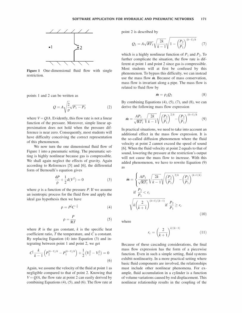
Consider a simple hydraulic setting with a single

restriction and the fluid is assumed to be noncom-

pressible. This setting is illustrated in Figure 1.

We shall neglect the effects of gravity and assume

the velocity of the fluid at point 1 as negligible com-

pared to that at point 2. Using Bernoulli’s equation,

we have according to Reference [5]

P1 ¼ P2 þ1

2rV2

2 ð1Þ

where Pi is the pressure at point i, Vi is the velocity of

the fluid and r its density. If we consider that the

opening surface at point 2 is A then the relation be-

tween the flow rate Q and the pressure difference at

170 WONG, BIGRAS, AND CERVERA

points 1 and 2 can be written as

Q ¼ A

ffiffiffi2

r

s ffiffiffiffiffiffiffiffiffiffiffiffiffiffiffiffiP1 � P2

pð2Þ

where V¼Q/A. Evidently, this flow rate is not a linear

function of the pressure. Moreover, simple linear ap-

proximation does not hold when the pressure dif-

ference is near zero. Consequently, most students will

have difficulty conceiving the correct representation

of this phenomenon.

We now turn the one dimensional fluid flow of

Figure 1 into a pneumatic setting. The pneumatic set-

ting is highly nonlinear because gas is compressible.

We shall again neglect the effects of gravity. Again

according to References [5] and [6], the differential

form of Bernoulli’s equation gives

dP

rþ 1

2dðV2Þ ¼ 0 ð3Þ

where r is a function of the pressure P. If we assume

an isentropic process for the fluid flow and apply the

ideal gas hypothesis then we have

r ¼ P1kC�

1k ð4Þ

r ¼ P

RTð5Þ

where R is the gas constant, k is the specific heat

coefficient ratio, T the temperature, and C a constant.

By replacing Equation (4) into Equation (3) and in-

tegrating between point 1 and point 2, we get

C1k

k

k � 1Pðk�1Þ=k2 � P

ðk�1Þ=k1

� �þ 1

2V22 � V2

1

� �¼ 0

ð6Þ

Again, we assume the velocity of the fluid at point 1 as

negligible compared to that of point 2. Knowing that

V¼Q/A, the flow rate at point 2 can easily derived by

combining Equations (4), (5), and (6). The flow rate at

point 2 is described by

Q2 ¼ AffiffiffiffiffiffiffiffiRT1p

ffiffiffiffiffiffiffiffiffiffiffi2k

k � 1

r ffiffiffiffiffiffiffiffiffiffiffiffiffiffiffiffiffiffiffiffiffiffiffiffiffiffiffiffiffiffiffiffiffi1� P2

P1

� �ðk�1Þ=ksð7Þ

which is a highly nonlinear function of P1 and P2. To

further complicate the situation, the flow rate is dif-

ferent at point 1 and point 2 since gas is compressible.

Most students will at first be confused by this

phenomenon. To bypass this difficulty, we can instead

use the mass flow _mm. Because of mass conservation,

mass flow is invariant along a pipe. The mass flow is

related to fluid flow by

_mm ¼ r2Q2 ð8Þ

By combining Equations (4), (5), (7), and (8), we can

derive the following mass flow expression

_mm ¼ AP1ffiffiffiffiffiffiffiffiRT1p


k � 1

r ffiffiffiffiffiffiffiffiffiffiffiffiffiffiffiffiffiffiffiffiffiffiffiffiffiffiffiffiffiffiffiffiffiffiffiffiffiffiffiffiffiffiffiffiffiP2

P1

� �2=k

� P2

P1

� �ðkþ1Þ=ksð9Þ

In practical situations, we need to take into account an

additional effect in the mass flow expression. It is

the so-called diffusion phenomenon where the fluid

velocity at point 2 cannot exceed the speed of sound

[6]. When the fluid velocity at point 2 equals to that of

sound, lowering the pressure at the restriction’s output

will not cause the mass flow to increase. With this

added phenomenon, we have to rewrite Equation (9)

as

_mm ¼ AP1ffiffiffiffiffiffiffiffiRT1p


k � 1

r ffiffiffiffiffiffiffiffiffiffiffiffiffiffiffiffiffiffiffiffiffiffiffiffiffiffiffiffiffiffiffiffiffiffiffiffiffiffiffiffiffiffiffiffiffiP2

P1

� �2=k

� P2

P1

� �ðkþ1=kÞs8<:if

P2

P1

< rcffiffiffiffiffiffiffiffiffiffiffiffiffiffiffiffiffiffiffiffiffiffiffiffiffiffiffiffiffiffiffiffiffiffiffiffiffiffiffik

2

k þ 1

� �ðkþ1Þ=ðk�1Þsif

P2

P1

� rc

ð10Þ

where

rc ¼2

k þ 1

� �k=ðk�1Þð11Þ

Because of these cascading considerations, the final

mass flow expression has the form of a piecewise

function. Even in such a simple setting, fluid systems

exhibit nonlinearity. In a more practical setting where

basic fluid components are involved, the relationships

must include other nonlinear phenomena. For ex-

ample, fluid accumulation in a cylinder is a function

of volume variations caused by rod displacement. This

nonlinear relationship results in the coupling of the

Figure 1 One-dimensional fluid flow with single

restriction.

SOFTWARE APPLICATION FOR HYDRAULIC AND PNEUMATIC NETWORKS 171

fluid part and the mechanical part of the system.

Furthermore, the mechanical part also possesses

nonlinear characteristics such as finite piston length,

static and dynamic frictions. All these nonlinear

characteristics and phenomena contribute to the

overall complexity of most simple fluid systems.

FLUID SYSTEM MODELING

In order to obtain an effective software application for

hydraulic and pneumatic network visualization and

understanding, it is necessary to employ a systematic

and efficient approach for its design and implemen-

tation. By modeling all hydraulic, pneumatic, and

mechanical components as multi-port devices, one

can apply the bond graph theoretic approach for net-

work topological recognition [7,8]. The bond graph

approach is a general technique that results in

system equation formulation. It is well suited for

hydraulic, pneumatic, and general mechanical sys-

tems because of its so-called causality analysis

capability [9].

In this design approach, all components are

modeled as multi-port devices. There are two vari-

ables associated with each device port. They represent

the effort-quantity (pressure, force, etc.) and the flow-

quantity (flow, speed, etc.) of the device. However

device port’s directional information is not known a

priori. That is, input-output relationship of the device

ports is dependent on the network’s topology. By

using bond graph’s causality analysis technique, one

can determine input-output relationship of every con-

nected port online.

The goal of bond graphs is to represent a dynamic

system by means of basic multi-port devices and their

interconnections by bonds. These basic multi-ports

exchange and modulate power through their bonds.

There exist two power variables and two correspond-

ing energy variables on each connected bond. They

are: (i) effort variable e(t)—pressure (force); (ii) flow

variable i(t)—flow rate (velocity); (iii) momentum

f(t)—pressure momentum; (iv) displacement variable

q(t)—volume. The effort variable is the time deriva-

tive of some momentum and conversely, the momen-

tum is the time integral of an effort,

eðtÞ ¼ dfðtÞ=dt; fðtÞ ¼ f0 þZ

eðtÞdt ð12aÞ

The same relationship applies to the flow variable and

the displacement variable,

iðtÞ ¼ dqðtÞ=dt; qðtÞ ¼ q0 þZ

iðtÞdt ð12bÞ

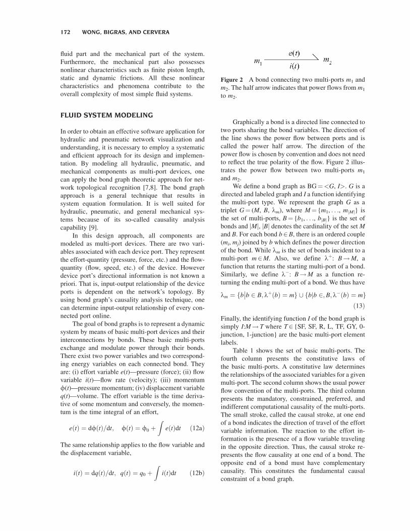
Graphically a bond is a directed line connected to

two ports sharing the bond variables. The direction of

the line shows the power flow between ports and is

called the power half arrow. The direction of the

power flow is chosen by convention and does not need

to reflect the true polarity of the flow. Figure 2 illus-

trates the power flow between two multi-ports m1

and m2.

We define a bond graph as BG¼<G, I>. G is a

directed and labeled graph and I a function identifying

the multi-port type. We represent the graph G as a

triplet G¼ (M, B, lm), where M¼ {m1, . . ., mjMj} is

the set of multi-ports, B¼ {b1, . . ., bjBj} is the set of

bonds and jMj, jBj denotes the cardinality of the setMand B. For each bond b2B, there is an ordered couple(mi, mj) joined by b which defines the power direction

of the bond. While lm is the set of bonds incident to a

multi-port m2M. Also, we define lþ: B!M, a

function that returns the starting multi-port of a bond.

Similarly, we define l�: B!M as a function re-

turning the ending multi-port of a bond. We thus have

lm ¼ fb b 2 B; lþðbÞ ¼ mg [ fb b 2;B;l�ðbÞ ¼ mgj��

ð13Þ

Finally, the identifying function I of the bond graph is

simply I:M! T where T2 {SF, SF, R, L, TF, GY, 0-junction, 1-junction} are the basic multi-port element

labels.

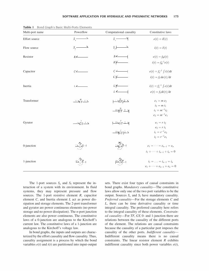
Table 1 shows the set of basic multi-ports. The

fourth column presents the constitutive laws of

the basic multi-ports. A constitutive law determines

the relationships of the associated variables for a given

multi-port. The second column shows the usual power

flow convention of the multi-ports. The third column

presents the mandatory, constrained, preferred, and

indifferent computational causality of the multi-ports.

The small stroke, called the causal stroke, at one end

of a bond indicates the direction of travel of the effort

variable information. The reaction to the effort in-

formation is the presence of a flow variable traveling

in the opposite direction. Thus, the causal stroke re-

presents the flow causality at one end of a bond. The

opposite end of a bond must have complementary

causality. This constitutes the fundamental causal

constraint of a bond graph.

Figure 2 A bond connecting two multi-ports m1 and

m2. The half arrow indicates that power flows from m1

to m2.


The 1-port sources Se and Sf represent the in-

teraction of a system with its environment. In fluid

systems, they may represent pressure and flow

sources. The 1-port resistive element R, capacitor

element C, and Inertia element L act as power dis-

sipation and storage elements. The 2-port transformer

and gyrator are power continuous elements (no power

storage and no power dissipation). The n-port junction

elements are also power continuous. The constitutive

laws of a 0-junction are analogous to the Kirchoff’s

current law. The constitutive laws of a 1-junction are

analogous to the Kirchoff’s voltage law.

In bond graphs, the inputs and outputs are charac-

terized by the effort causality and flow causality. Thus,

causality assignment is a process by which the bond

variables e(t) and i(t) are partitioned into input-output

sets. There exist four types of causal constraints in

bond graphs. Mandatory causality—The constitutive

laws allow only one of the two port variables to be the

output. Sources Se and Sf have mandatory causality.

Preferred causality—For the storage elements C and

L, there can be time derivative causality or time

integral causality. The preferred causality here refers

to the integral causality of these elements. Constrain-

ed causality—For TF, GY, 0- and 1-junction there are

relations between the causality of the different ports

of the element. The relations are causal constraints

because the causality of a particular port imposes the

causality of the other ports. Indifferent causality—

Indifferent causality means there is no causal

constraints. The linear resistor element R exhibits

indifferent causality since both power variables e(t),

Table 1 Bond Graph’s Basic Multi-Ports Elements

Multi-port name Powerflow Computational causality Constitutive laws

Effort source eðtÞ ¼ EðtÞ

Flow source iðtÞ ¼ IðtÞ

Resistor eðtÞ ¼ fRiðtÞ

iðtÞ ¼ f�1R eðtÞ

Capacitor eðtÞ ¼ f�1C

RiðtÞdt

iðtÞ ¼ fCdeðtÞ=dt

Inertia iðtÞ ¼ f�1L

ReðtÞdt

eðtÞ ¼ fLdiðtÞ=dt

Transformer e1 ¼ m e2

i2 ¼ m i1

i1 ¼ m�1i2

e2 ¼ m�1e1

Gyrator e1 ¼ r i2

e2 ¼ r i1

i1 ¼ r�1e2

i2 ¼ r�1e1

0-junction e1 ¼ � � � ¼ en�1 ¼ en

i1 þ � � � þ in�1 þ in ¼ 0

1-junction i1 ¼ . . . ¼ in�1 ¼ in

e1 þ � � � þ en�1 þ en ¼ 0


i(t) can be made member of the input and output

sets.

Most traditional causality assignment procedures

use a local constraint propagation scheme to label

bond causality. From some starting point, usually one

of the source elements, bond causality is assigned

sequentially, according to the multi-port connected to

the bond, until all element ports are labeled. These

causality assignment procedures must also satisfy the

four causality types and the fundamental causal con-

straint.

The sequential causality assignment procedure or

SCAP is an example of causal labeling by local

propagation [9]. The following pseudocode describes

the causality assignment procedure.

Procedure SCAP: input(BG), output(BG)

P M

while (jP j> 0) {

x m, where I(m)¼ SE_ I(m)¼ SF

if ({x}¼¼Ø)

x m, where I(m)¼C_ I(m)¼L

if ({x}¼¼Ø)

x m, where I(m)¼R

P¼P� { m }

assign(x, lx)If conflict(BG) abort

If complete(BG) return BG

}

The assign(x, lx) procedure selects the appro-

priate mandatory, preferred, or constrained causality

(shown in Table 1) for multi-port x. It also attempts to

assign causality to transformer, gyrator, and n-port

junction elements that are connected to x by using the

set of bonds lx. After the assign procedure, a check is

made to ensure that no causal conflict exists in the

bond graph. Otherwise, the procedure will abort.

Normally a causal conflict indicates the presence of

topological loops (differential/algebraic loops), de-

pendent storage elements, or simply design errors.

Such degenerated networks produce a set of differ-

ential algebraic equations and its solution is often

time consuming. More details on causality assignment

techniques can be found in References [9,10].

State-Space Formulation

For each causality, the numerical model of the i-th

component is a nonlinear ODE system of form

_xxi ¼ hiðxiÞ þ biðxi; uiÞyi ¼ giðxiÞ þ diðxi;uiÞ

ð14Þ

where xi is the state vector, yi is the outputs vector andui is the inputs of the i-th component. Using the par-

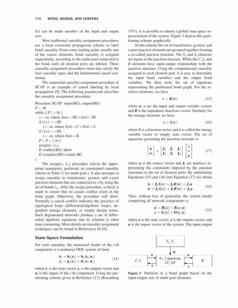
titioning scheme given in Reference [11] (Rosenberg

1971), it is possible to obtain a global state-space re-

presentation of the system. Figure 3 depicts this parti-

tioning scheme graphically.

In this scheme the set of transformer, gyrator, and

n-port junction elements are grouped together forming

a so-called junction structure. The Se and Sf elements

are inputs to the junction structure. While the C, L, and

R elements have input-output relationships with the

junction structure. Using the computational causality

assigned to each element port, it is easy to determine

the input bond variables and the output bond

variables. We then write the set of equations

representing the partitioned bond graph. For the re-

sistive elements, we have

v ¼ RðwÞ ð15Þ

where w, v are the input and output variable vectors

and R is the impedance functions vector. Similarly for

the storage elements we have

z ¼ SðxÞ ð16Þ

where S is a function vector and x is called the energyvariable vector or simply state vector. The set of

equations governing the junction structure is

_xxw

¼ J1 J2 J3

J4 J5 J6

zvu

24

35 ð17Þ

where u is the source vector and Ji are matrices re-

presenting the constraints imposed by the junction

structures to the set of element ports. By substituting

Equations (15) and (16) into Equation (17) we obtain

_xx ¼ J1SðxÞ þ J2RðwÞ þ J3uw ¼ J4SðxÞ þ J5RðwÞ þ J6u

ð18Þ

Thus, without loss of generality, the system model

comprising all network components is

_xx ¼ HðxÞ þ Bðx; uÞy ¼ GðxÞ þ Dðx; uÞ ð19Þ

where x is the state vector, y is the outputs vector, andu is the inputs vector of the system. The input-output

Figure 3 Partition of a bond graph based on the

input-output sets of multi-port elements.


coupling between network components can be model-

ed as

u ¼ Cy ð20Þ

Finally, the global model of all interconnected com-

ponents is obtained by substituting Equation (20) into

Equation (19). Since there is no algebraic loop, the

model can then be written as follows:

_xx ¼ HðxÞ ð21aÞ

y ¼ GðxÞ ð21bÞ

We can consider the system equations as an

assembly of two coupled subsystems: one depicting

the slow-varying part and the other depicting the fast-

varying part of the system. In physical terms, the

slow-varying part represents the mechanical interac-

tions and the elasticity of the pneumatic fluid. Using

similar reasoning, the fast-varying part represents the

elasticity of the hydraulic fluid. By applying the

singular perturbation approach [12], the global model

can then be rewritten as:

_xxs ¼ Hsðxs; xfÞ ð22aÞ

e _xxf ¼ Hfðxs; xfÞ ð22bÞ

y ¼ Gðxs; xfÞ ð22cÞ

where xs and xf are the vectors of the state variables

associated to the slow and fast subsystems and e is asmall positive parameter associated to the time con-

stant of the fast subsystem. Since the parameter e is

close to zero, a good approximation solution of the

slow subsystem can be obtained by posing e¼ 0. The

global model is then given by

_xxs ¼ Hsðxs; xf Þ ð23aÞ

0 ¼ Hf ðxs; xf Þ ð23bÞ

y ¼ Gðxs; xfÞ ð23cÞ

In this model, the set of nonlinear differential

equations of the fast varying part is transformed into

a set of nonlinear algebraic equation [12]. This result

greatly facilitates the construction of the numerical

integrator that can operate in quasi real-time. An

adaptive integrator, part of the software application

subsystems, is used to ensure the accuracy of the

solution at each time-step. Note that the global model

includes a static part (23b) and a dynamic part (23a).

The integrator with adaptive time-steps is based on

multiple evaluations of the model. At each model

evaluation, the static part must be solved. This

approach allows us to have a larger time-step since

only the slow subsystem must be integrated. However,

because the latter is iterative in nature, it is not

possible to guarantee hard real-time performance.

DESIGN AND IMPLEMENTATION

In the proposed software application, the process of

construction, simulation and data display is a set of

simple tasks. In the construction task, hydraulic,

pneumatic, and mechanical components are selected

from the component palettes. Using hydraulic (pneu-

matic) links and connecting them to component ports,

one can create component interconnections to form a

network. Each network component contains a numer-

ical model whose parameters are adjustable via the

user interface. A student can accept the default values,

use specific settings given by instructor or specify

values directly from manufacturer’s data sheets. For

the simulation task, numerical simulation is perform-

ed in either continuous mode or step-by-step mode. In

continuous mode, system equations solution and

graphical animation updates are continuously execut-

ed every time-step. In step-by-step mode, the student

is responsible for time-step increment (by depressing

a key or a mouse click) so that it is possible to slow

down or speed up the simulation process. Finally, the

data display task consists of data collection using

measurement components. Data are displayed syn-

chronously with the simulator output in both numer-

ical and graphical forms. Data collected are persistent

until the next simulation run. The measurement com-

ponents can also perform formatted storage opera-

tions. This enables extensive post-simulation analysis

using external data analysis tools.

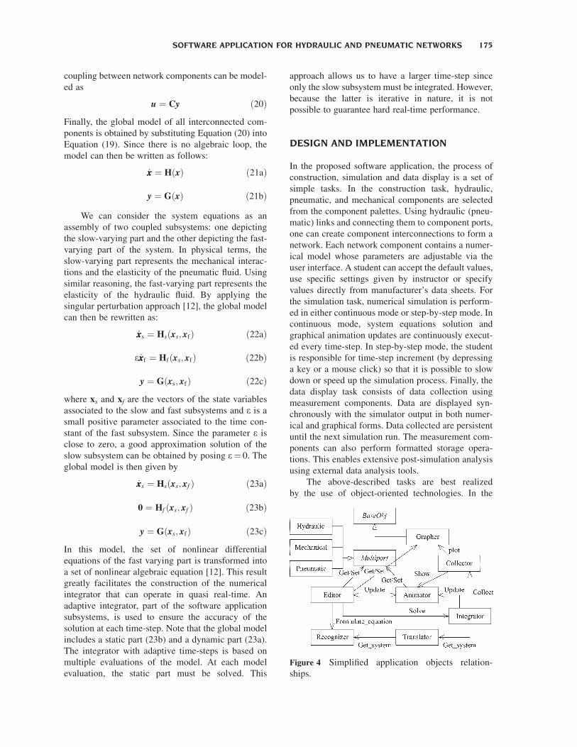
The above-described tasks are best realized

by the use of object-oriented technologies. In the

Figure 4 Simplified application objects relation-

ships.


object-oriented approach, a software application is the

result of a collection of cooperating objects [13,14].

We obtain the objects for the software application by

analyzing its specification along a responsibility as-

signment point of view [15]. Thus, all objects must

have non-trivial responsibilities assigned to them.

Otherwise they are discarded from the design.

In-simulation Interactions

As shown in Figure 4, there is a logical interface

between the integrator output and the graphical

animation subsystem. The latter subsystem is respon-

sible for updating color changes and the rendering of

moving parts on behalf of the network components.

The graphical animation subsystem also collaborates

closely with network components and the network

editor to allow in-simulation interactions. An in-

simulation interaction permits a student to change or

modify a component’s state while a simulation run is

in progress. Thus, the student can stop or start motors,

select different distributor pistons, modify cylinder’s

longitudinal position and so on.

In order to allow in-simulation interactions, the

application establishes a so-called mechanical chain

to determine the effect of changes on other network

components. This involves the recalculation of net-

work states and their propagation to all connected

components by a graph traversal. To implement in-

simulation interactions every network component that

possesses user-interactivity must register itself with an

object called in-simulation observer. During a simula-

tion run, all mouse and keyboard events (or simply

user events) are filtered and routed to the in-

simulation observer. The observer passes along the

user events to the registered components. Consequent-

ly, it is the network components that are responsible

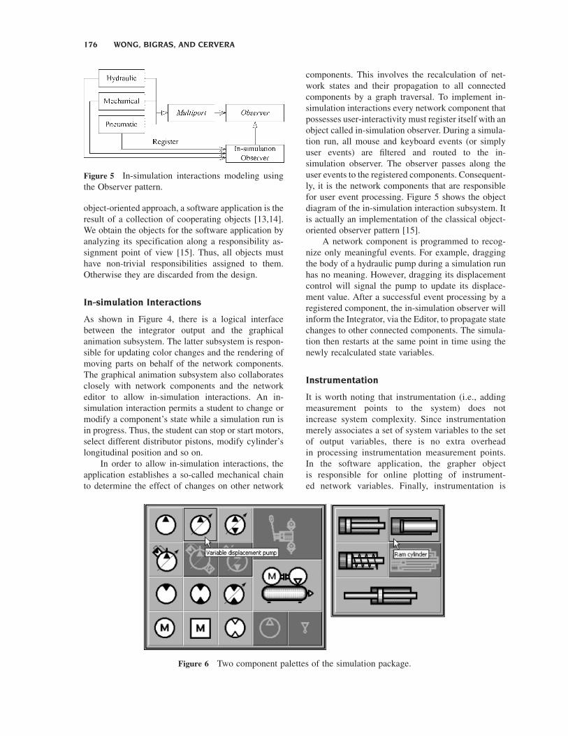
for user event processing. Figure 5 shows the object

diagram of the in-simulation interaction subsystem. It

is actually an implementation of the classical object-

oriented observer pattern [15].

A network component is programmed to recog-

nize only meaningful events. For example, dragging

the body of a hydraulic pump during a simulation run

has no meaning. However, dragging its displacement

control will signal the pump to update its displace-

ment value. After a successful event processing by a

registered component, the in-simulation observer will

inform the Integrator, via the Editor, to propagate state

changes to other connected components. The simula-

tion then restarts at the same point in time using the

newly recalculated state variables.

Instrumentation

It is worth noting that instrumentation (i.e., adding

measurement points to the system) does not

increase system complexity. Since instrumentation

merely associates a set of system variables to the set

of output variables, there is no extra overhead

in processing instrumentation measurement points.

In the software application, the grapher object

is responsible for online plotting of instrument-

ed network variables. Finally, instrumentation is

Figure 5 In-simulation interactions modeling using

the Observer pattern.

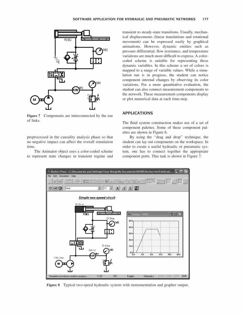
Figure 6 Two component palettes of the simulation package.


preprocessed in the causality analysis phase so that

no negative impact can affect the overall simulation

time.

The Animator object uses a color-coded scheme

to represent state changes in transient regime and

transient to steady-state transitions. Usually, mechan-

ical displacements (linear translations and rotational

movement) can be expressed easily by graphical

animations. However, dynamic entities such as

pressure differential, flow resistance, and temperature

variations are much more difficult to express. A color-

coded scheme is suitable for representing these

dynamic variables. In this scheme a set of colors is

mapped to a range of variable values. While a simu-

lation run is in progress, the student can notice

component internal changes by observing its color

variations. For a more quantitative evaluation, the

student can also connect measurement components to

the network. These measurement components display

or plot numerical data at each time-step.

APPLICATIONS

The fluid system construction makes use of a set of

component palettes. Some of these component pal-

ettes are shown in Figure 6.

By using the ‘‘drag and drop’’ technique, the

student can lay out components on the workspace. In

order to create a useful hydraulic or pneumatic sys-

tem, one has to connect together the appropriate

component ports. This task is shown in Figure 7.

Figure 7 Components are interconnected by the use

of links.

Figure 8 Typical two-speed hydraulic system with instrumentation and grapher output.


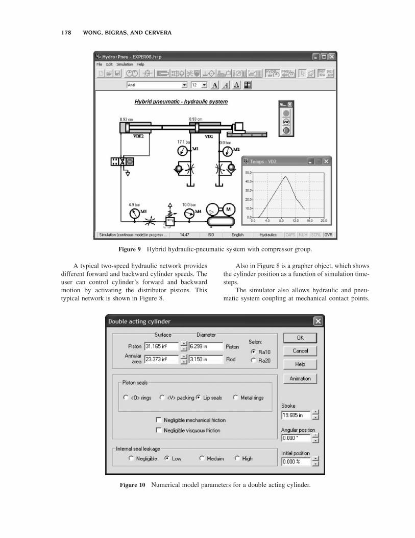
A typical two-speed hydraulic network provides

different forward and backward cylinder speeds. The

user can control cylinder’s forward and backward

motion by activating the distributor pistons. This

typical network is shown in Figure 8.

Also in Figure 8 is a grapher object, which shows

the cylinder position as a function of simulation time-

steps.

The simulator also allows hydraulic and pneu-

matic system coupling at mechanical contact points.

Figure 9 Hybrid hydraulic-pneumatic system with compressor group.

Figure 10 Numerical model parameters for a double acting cylinder.


This capability permits the study of different system

dynamics and their interplay. In Figure 9, the mech-

anical contact point is the interface between the

pneumatic and hydraulic cylinders. This hybrid net-

work shows an interesting application where a pneu-

matic cylinder, driven by its compressor group, is the

prime moving force.

The hydraulic cylinder, which is coupled to the

pneumatic one, acts as a retaining force on behalf of

the load. Note that this hybrid configuration offers

different retaining force for forward and backward

cylinder motions since there is two flow controls

installed on the hydraulic cylinder. Again, the student

can control forward or backward motion by activating

the distributor pistons or by dragging one of the

cylinder’s pistons.

As indicated earlier every hydraulic, pneumatic,

and mechanical component possesses a numerical

model that is fully adjustable. Figure 10 shows a

typical component dialog box for parameter input. In

most cases, non-ideal component characteristics are

possible. For example, Figure 10 depicts an input

dialog box for a double acting cylinder. The student

can select from several joint leak degrees (negligible,

low, medium, and high) to obtain non-ideal character-

istics caused by aging and wears of the component.

CONCLUSIONS

This study presented the motivation and the design of

a software application for visualizing and under-

standing hydraulic and pneumatic networks. The

intent is to help students analyze fluid system behav-

iors. This application is suitable for small-to-medium

scale fluid system analysis. It uses a combined bond

graph and singular perturbation approach for system

equation formulation. A standard adaptive integrator

solves the system equations that are divided into a

slow-varying part and a fast-varying part. The logical

interface of the integrator output and the graphical

animation and instrumentation subsystems are also

detailed in the study. The graphical animation sub-

system is responsible for updating color changes and

rendering of moving parts on behalf of network

components. An important feature of this computer

application is its ability to permit in-simulation in-

teractions. It allows the students to manipulate

network components while a simulation run is in

progress. This feature should facilitate hydraulic

and pneumatic network understanding by putting

the students in the simulation loop. Finally, this

software application is in use in number of univer-

sities and technical colleges throughout Quebec. It

has been awarded the Quebec Education Minister’s

Award for ‘‘best educational software’’ in the year

2000.

REFERENCES

[1] D. Cervera, Elaboration d’un environnement d’experi-

mentation en simulation, incluant un cadre theorique

pour l’apprentissage de l’energie des fluides. Ph.D.

Dissertation, faculte des sciences de l’education,

Universite de Montreal, 1998.

[2] D. Cervera and A. Metioui, Energie des fluides:

Analyse conceptuelle et representation des eleves,

technical report (PAREA), College de Valleyfield,

Quebec, 1993.

[3] A. Youssef, A. Metioui, P. Bigras, and D. Cervera, Les

representations des etudiants du collegial profession-

nel a l’egard des principes de fonctionnement des

circuits hydrauliques, technical report, Ecole de tech-

nologie superieure, University of Quebec, 1991.

[4] T. Wong, P. Bigras, and D. Cervera, A software tool for

understanding nonlinear phenomena in hydraulic and

pneumatic systems, Proceedings of the American

Society of Engineering Education Conference, session

2220, paper 514, 2002.

[5] R. R. Munson, D. F. Young, and T. H. Okiishi,

Fundamentals of fluid mechanics, Wiley, New York,

1998.

[6] B. W. Andersen, The analysis and design of pneumatic

systems, Wiley, New York, 1967.

[7] A. Mukherjee and R. Karmakar, Modeling and simu-

lation of engineering systems through bondgraphs,

CRC Press LLC, Boca Raton, FL, 2000.

[8] D. C. Karnopp, D. L. Margolis, and R. C. Rosenberg,

System dynamics: A unified approach, Wiley,

New York, 1990.

[9] J. D. Dijk, On the role of bond graph causality in

modelling mechatronic systems. Ph.D. Dissertation,

University of Twente, CIP-Gegevens, 1994.

[10] T. Wong, P. Bigras, and K. Khayati, Causality assign-

ment using multi-objective evolutionary algorithms,

IEEE Int Conf Syst, Man and Cybern 4 (2002), 36�41.[11] R. C. Rosenberg, State-space formulation for bond

graph models of multi-port systems, Transactions of

the ASME, J Dyn Syst Meas Control 93 (1971),

123�125.[12] H. K. Khalil, Nonlinear systems, Macmillan,

New York, 1992.

[13] J. Rumbaugh, M. Blaha, W. Premerlani, F. Eddy, and

W. Lorensen, Object-oriented modeling and design,

Prentice Hall, Englewood Cliffs, NJ, 1991.

[14] R. Allen, A formal approach to software architecture.

Ph.D. Dissertation, Carnegie Mellon University,

1997.

[15] A. Shalloway and R. Trott, Design patterns explained:

A new perspective on object-oriented design, Addison-

Wesley, New York, 2001.


BIOGRAPHIES

TonyWong holds BEng andMEng degrees

in electrical engineering from the Ecole de

Technologie Superieure. He received his

PhD in computer engineering from Ecole

Polytechnique de Montreal. Dr. Wong is a

professional engineer and chair of the

automated manufacturing engineering

department, Ecole de Technologie Super-

ieure. His current research interests are

multiobjective optimization using evolutionary algorithms and its

parallel implementations.

Pascal Bigras received the BEng degree in

electrical engineering and the MEng

degree from the Ecole de Technologie

Superieure of Montreal in 1991 and 1993,

respectively, and his PhD in automatic

control from Ecole Polytechnique de

Montreal in 1997. Dr. Bigras is an associate

professor at the Ecole de Technologie

Superieure. His current research interests

are simulation and nonlinear and robust control.

Daniel Cervera holds his PhD degree in

education sciences from Universite de

Montreal. Dr. Cervera has taught at College

de Valleyfield for the past 30 years. His

current research interests are in the field of

abstract representations of technical and

scientific knowledge.


Documents

A software application for visualizing and understanding hydraulic and pneumatic networks